Analysis and lattice Boltzmann simulation of thermoacoustic instability in a Rijke tube

Abstract

The combined effects of heater position, mean flow parameters and flame models on thermoacoustic instability in a one-dimensional Rijke tube are studied systematically by classic linear stability analysis (LSA) and lattice Boltzmann method (LBM) simulation. In the former, the stability range of the linear flame model under low Mach number assumption is solved analytically, while in the more general case, it is obtained by numerically solving the dispersion relation. Both the linear and nonlinear flame model cases are studied using the LBM with a spectral multiple-relaxation-time collision model and a newly developed heat source term. With the linear flame model, the LBM is in good agreement with LSA in predicting the transition point and growth rates, while with the nonlinear flame model, LBM simulations are consistent with solutions of limit cycle theory in the fully developed state. These results demonstrate the applicability of the LBM in solving complex thermoacoustic problems.

1. Introduction

Thermoacoustic instability (TAI) is a critical issue in propulsion engines as it may cause severe damage to an engine when excited to a large amplitude (Poinsot 2017). This instability results from the coupling between unsteady heat release and acoustic fluctuations, and has been studied extensively by a variety of approaches, such as simple analytical models (Hubbard & Dowling 2001), time-domain network models (Pankiewitz & Sattelmayer 2003; Stow & Dowling 2009), and more recently computational fluid dynamics (CFD) simulations (Hantschk & Vortmeyer 1999; Cannon, Adumitroaie & Smith 2001; Poinsot & Veynante 2005). In addition to the common difficulties in turbulence modelling, simulation of TAI with classic CFD methods is extremely demanding on computational resources due to its stiff characteristics involving drastically different spatial and temporal scales (Poinsot 2017). A realistic calculation requires a very high resolution to capture both the small flamelets and the large wavelength of the pressure waves. This causes a strict limitation on time step in simulations, and usually a large number of numerical evolutions are necessary due to the considerably long time before the onset of self-sustaining instability (Toffolo, Masi & Lazzaretto 2010). These constraints require the numerical method to have both low dissipation and high efficiency as well as the ability to handle complex geometries for practical applications.

The Rijke tube is a greatly simplified piece of equipment that can reproduce the fundamental TAI phenomenon. It has been thoroughly studied in both experiments and theoretical analysis. In the idealized version shown in figure 1 (Matveev 2003; Xi et al. 2022), the flame is replaced by a heater to avoid complex chemical reaction processes. Due to its relative simplicity, a lot of work has been devoted to the analysis of the horizontal Rijke tube in the TAI study. The classic analytical approach is to apply the perturbation method in frequency space, and link the flow fluctuations to the heat release rate with a linear flame transfer function (FTF). The stability for each eigenfrequency can then be predicted (Dowling 1995). When the amplitude of oscillation increases, a nonlinear flame describing function (FDF) can be used to replace the linear FTF so that the limit cycle oscillations and their frequencies can be described correctly (Dowling 1997, 1999; Stow & Dowling 2004; Noiray et al. 2008). However, this ‘describing function’ approach is applicable only when there is one dominant mode. To overcome this shortcoming, Stow & Dowling (2009) proposed a time domain analytical approach that transforms FDFs into temporal space first, and then uses convolution integration with time to dispose the interaction of different modes. This method has been further developed to explain phenomena known as hysteresis, triggering, mode switching and frequency shift during the growth of instabilities (Noiray et al. 2008; Boudy et al. 2011, 2013; Palies et al. 2011).

Figure 1. Demonstration of a horizontal Rijke tube with a compact heater (the red dashed line), and the coordinate definition. We take the integration of $u'$ and $p'$ in analysis infinitesimal control volume around the compact flame model (the green dash-dotted box) to get the connecting condition. The volume thickness is $\delta x\to 0$. Subscripts 1 and 2 denote the upstream and downstream regions of the heater, respectively.

Although the analytical approach is rather successful, for practical combustors the multi-dimensional effects and complex geometry make the analysis difficult. Consequently, several groups tried to employ the classic CFD simulation to solve thermal acoustic problems. Hantschk & Vortmeyer (1999) used the commercial software Fluent to simulate the self-excited thermoacoustic instabilities in Rijke tubes. Cannon et al. (2001) simulated the lean premixed fuel combustors by three-dimensional RANS and LES models with a Fluent-like pressure-based finite volume solver. Mariappan & Sujith (2011) used the similar CFD algorithm in the hydrodynamic zone near the heater, and performed the Galerkin technique for the acoustic zone far away. Generally speaking, the traditional CFD methods are still suffering from the stiff problem due to the scale separation between the heat source and acoustic waves at present.

Over the past few decades, the lattice Boltzmann method (LBM) (Benzi, Succi & Vergassola 1992; Chen & Doolen 1998) has attracted tremendous attention in the CFD community. Unlike traditional methods that solve the Navier–Stokes equation with macroscopic variables directly, the LBM solves a discrete version of the Boltzmann equation on a mesoscopic scale, with which the Navier–Stokes macroscopic behaviours or even those beyond may be described adequately. This allows certain subtle physical mechanisms to be included in calculations at a more fundamental level. Furthermore, the LBM is inherently parallelizable and can easily exploit the vast computational resource available on modern GPU (Kuznik et al. 2010; Rinaldi et al. 2012; Wang et al. 2014; Delgado-Gutierrez et al. 2020). For computational aero-acoustics, many studies have shown its low dissipation and high efficiency (Buick, Greated & Campbell 1998; Marié, Ricot & Sagaut 2009; Barad, Kocheemoolayil & Kiris 2017), which makes the LBM a promising method for simulating acoustic problems.

The LBM simulation of the highly thermally compressible flow in engine TAI is still considered difficult to a large extent. This is partly due to the fact that the LBM was originally developed a posteriori (Chen, Chen & Matthaeus 1992; Qian, d'Humières & Lallemand 1992) to ensure that its macroscopic behaviour follows the near-incompressible Navier–Stokes equation. Efforts to extend this approach to thermal flows have encountered difficulties in recovering the energy equation with sufficient numerical stability (McNamara, Garcia & Alder 1995). In addition to the lack of energy conservation, the non-thermal LBM suffers from a number of artefacts, including the velocity-dependent viscosity, the isothermal (Newtonian) sound, the unity Prandtl number, and the fixed and incorrect isentropic indices, all of which can be significant obstacles in TAI simulations.

Nowadays, in general two categories of LBM are developed to treat thermal flow. The most common approach is to use the athermal LBM to solve the continuity and momentum equations, and another LBM or other traditional solver to resolve the energy (or equivalently temperature, pressure, entropy, etc.). For instance, Wang et al. (2015) has simulated the open–open Rijke tube with a hybrid finite-difference, double-distribution LBM, and this approach was followed recently by Slimene et al. (2022). In these non-thermal LBM solvers, the compressible and thermal effects have to be explicitly patched and modelled. Although conceptually simple, this type of approach has the disadvantage that the patching and modelling must be done case by case, and are seldom complete.

The other type of thermal LBM attempts to naturally restore the energy equation as the second-order moment equation of the Boltzmann equation (Alexander et al. 1992; Chen, Ohashi & Akiyama 1994; McNamara et al. 1995). Early attempts of this kind treated the LBM as a kinetic description of a discrete system, and were not very satisfactory due to the lack of clear theoretical guidance. Later theory of formulating the LBM as a velocity–space discretization (Shan & He 1998; Shan, Yuan & Chen 2006) gave the necessary and sufficient conditions for the various hydrodynamic moments to be recovered in the LBM (Nie, Shan & Chen 2008a). Very recently, the spectral multiple-relaxation-time (SMRT) collision model (Li & Shan 2021; Shan, Li & Shi 2021) addressed additional compressible artefacts and has theoretically enabled LBM simulations of thermal compressible flows with correct Prandtl numbers and isentropic exponents.

During the same period, another type of thermal LBM model, based on a body-centred-cubic lattice, was proposed by Namburi, Krithivasan & Ansumali (2016), which used two usual lattices displaced by an offset distance of half the mesh size in each direction. This lattice can provide better accuracy in both the spatial and velocity spaces, and works well for high Rayleigh number flows (Atif, Namburi & Ansumali 2018). Recently, Kolluru, Atif & Ansumali (2023) combined the body-centred-cubic lattice model with an advection–diffusion relaxation equation for the rotational energy to allow tunable bulk viscosity, thermal conductivity and specific heat ratio, and satisfactory results were obtained in benchmarks for polyatomic gases.

To the best of our knowledge, few works have applied the advantage of the LBM in acoustic computation to thermoacoustic problems. The published works that are related to this topic, i.e. Wang et al. (2015) and Slimene et al. (2022), have adopted a block heater with high temperature in the tube to provide the heat source. This is rather different from the realistic heater that has infinitely thin thickness in laboratory TAI equipment or gas turbines. The present work aims at validating and further developing the LBM, especially with the SMRT model, for simulation of TAI using the compact flame model in a Rijke tube as the benchmark. In § 2, the approach of linear stability analysis (LSA) is adopted to obtain the transition point and growth rate for different heater locations and other flow parameters with a linear flame model. This detailed analysis has merely been elaborated in the past studies, and the results will also be used as reference to validate the accuracy of the thermal LBM. In § 3, a number of Rijke flow cases with linear flame model are simulated by the LBM using a heat source model and modified reflecting boundary condition. The comparison of LSA and LBM simulation results will also be presented. Next, the LBM is applied to the Rijke tube with a nonlinear flame model in § 4. A brief conclusion is given in § 5.

2. Thermoacoustic theory in a Rijke tube

A typical horizontal Rijke tube is illustrated in figure 1. The gas flow with density $\rho$, velocity $u$ and temperature $T$ enters the tube from the left, passes through an infinitely thin heater located at $x=0$ with a heat release rate per unit area of $Q$, and forms a downstream flow with a discontinuity at the flame. Neglecting transverse and viscous effects, the flow in the duct can be described by the one-dimensional Euler equation:

(2.1) \begin{equation} \left. \begin{gathered} {\dfrac{\partial \rho}{\partial t}} + {\dfrac{\partial {(\rho u)}}{\partial x}} = 0, \\ {\dfrac{\partial {(\rho u)}}{\partial t}} + {\dfrac{\partial {(\rho u^2+p)}}{\partial x}} = 0, \\ {\dfrac{\partial {(\rho E)}}{\partial t}} + {\dfrac{\partial {(\rho Eu+pu)}}{\partial x}} = Q. \end{gathered} \right\} \end{equation}

Here, $E=e+u^2/2$, with $e=RT/(\gamma -1)$ being the internal energy, $R$ the gas constant, and $\gamma$ the specific heat ratio. The physical variables are non-dimensionalized as follows. Given the reference temperature $T_0$ and density $\rho _0$ – usually the values at the upstream inlet – the reference speed is $V_0 = \sqrt {R T_0}$. Choosing the reference length $L_0$ as the grid size $\Delta x$ of the LBM simulation, the reference time scale is $t_0=L_0/V_0$. The reference pressure is defined as $p_0=\rho _0 V_0^2$ so that the ideal gas law can be written as $p=\rho T$ in non-dimensional form. The non-dimensional heat source term is $Q^\ast = Q\rho _0 V_0^3/L_0$. If we omit the superscript $\ast$, then the non-dimensional Euler equation has exactly the same form as (2.1). Hereinafter, all quantities are in non-dimensional form.

We decompose the flow parameters into the mean and fluctuation parts, e.g. $\rho (x,t)=\bar {\rho }+\rho '(x,t)$, and the same goes for $u$, $p$, $T$ and $Q$. Here, we omit the subscripts $j=1,2$ shown in figure 1 for brevity. Further, assuming that the mean quantities of the fully developed flow are time-independent, the fluctuations are governed by the linearized Euler equation for both the upstream and downstream flows, with the mean quantities taking their corresponding values:

(2.2a, 2.2b, 2.2c and 2.2d) $$\begin{cases}{} \dfrac{\partial \rho'}{\partial t}+\bar{u}\,\dfrac{\partial\rho'}{\partial x}+\bar{\rho}\,\dfrac{\partial u'}{\partial x}= 0,\\ \dfrac{\partial u'}{\partial t}+\bar{u}\,\dfrac{\partial u'}{\partial x}+\dfrac{1}{\bar{\rho}}\,\dfrac{\partial p'}{\partial x}= 0,\\ \dfrac{\partial T'}{\partial t} +\bar{u}\,\dfrac{\partial T'}{\partial x}+(\gamma-1)\bar{T}\,\dfrac{\partial u'}{\partial x}=Q',\\ \dfrac{\partial p'}{\partial t} +\bar{u}\,\dfrac{\partial p'}{\partial x}+\gamma\bar{p}\,\dfrac{\partial u'}{\partial x}=(\gamma-1)Q'.\end{cases}$$

Defining the material derivative operator $\mathrm {D} / \mathrm {D}t = \partial /\partial t+\bar {u}\partial /\partial x$ and applying it to (2.2d), with the help of (2.2b), we have the wave equation

(2.3)\begin{equation} \frac{1}{\bar{c}^2}\,\frac{\mathrm{D}^2p'}{\mathrm{D}t^2} - \frac{\partial^2p'}{\partial x^2} = \frac{\gamma-1}{\bar{c}^2}\,\frac{\mathrm{D}Q'}{\mathrm{D}t}, \end{equation}

where $\bar {c}=\sqrt {\gamma \bar {p}/\bar {\rho }}$ is the sound speed.

In the following, we first derive the relations connecting the mean and fluctuation variables across the heater using the flame models. Then, with different simplifications (e.g. with or without the low Mach number assumption), LSA will be performed to obtain the dispersion relation from which the temporal growth characteristics of the acoustic waves can be discerned. These growth features will provide reference for the LBM simulation detailed in the next section.

2.1. Connecting relations and flame model

As shown in figure 1, the compact flame model $Q(x,t)=Q(t)\,\delta (x)$ is positioned at $x=0$. The integration of the Euler equation (2.1) over the infinitely thin control volume across the heater results in

(2.4a, 2.4b and 2.4c) $$\begin{cases} \bar{\rho}_1 \bar{u}_1 = \bar{\rho}_2 \bar{u}_2, \\ \bar{p}_1 + \bar{\rho}_1 \bar{u}^2_1 = \bar{p}_2 + \bar{\rho}_2 \bar{u}_2^2, \\ \bar{u}_1(\bar{\rho}_1 \bar{E}_1+\bar{p}_1)+\bar{Q} = \bar{u}_2(\bar{\rho}_2 \bar{E}_2+\bar{p}_2).\end{cases}$$

Combining (2.4a) and (2.4b) with $\bar {p}_j=\bar {\rho }_j \bar {T}_j$, we have

(2.5)\begin{equation} \bar{u}^2_2-\frac{\bar{T}_1+\bar{u}_1^2}{\bar{u}_1}\,\bar{u}_2+\bar{T}_2=0. \end{equation}

Practically, we typically prescribe $\bar {\rho }_1$, $\bar {u}_1$, $\bar {T}_1$ and a desired $\bar {T}_2$, from which $\bar {u}_2$ can be solved using (2.5). Then $\bar {\rho }_2$ and $\bar {Q}$ can be obtained from (2.4a) and (2.4c), thus all the downstream mean variables are determined. The connecting relations for the fluctuations can be derived by integrating (2.2b) and (2.2d) over the same control volume:

(2.6a)$$\begin{gather} \left[p' + \bar{\rho} \bar{u}u'\right]^{x=0^+}_{x=0^-} = 0, \end{gather}$$

(2.6b)$$\begin{gather}\left[\bar{u}p' + \gamma\bar{p}u'\right]^{x=0^+}_{x=0^-} = (\gamma-1)Q'. \end{gather}$$

The simplest unsteady heat release rate model is the time-lag (or $n$-$\tau$) model (Crocco 1951; Dowling & Stow 2003; Schuller, Poinsot & Candel 2020). In this model, $Q'$ depends only on the velocity $u^{\prime }_1$ at the heater position ($x=0$), as

(2.7)\begin{equation} Q'(x=0,t)=\frac{\bar{Q}}{\bar{u}_1}\,N u^{\prime}_1(x=0,t-\tau), \end{equation}

where $N$ measures the strength of the flame's response to the velocity perturbations, and $\tau$ is the time lag between $Q'$ and $u'$. These two parameters are constants, determined on a case-by-case basis by the flame's configuration. Transforming (2.7) into the frequency domain, we obtain

(2.8)\begin{equation} \frac{\hat{Q}'(\omega)}{\bar{Q}}=\int_{0}^{+\infty}N\, \frac{u^{\prime}_1(x=0,t-\tau)}{\bar{u}_1}\,{\rm e}^{\mathrm{i}\omega t}\,{\rm d}t=N\,{\rm e}^{-\mathrm{i}\omega\tau}\,\frac{\hat{u}^{\prime}_1 (\omega)}{\bar{u}_1}. \end{equation}

It can be observed that $\hat {Q}'$ can grow with $\hat {u}'$ at any frequency. However, according to the experiment of Bloxsidge, Dowling & Langhorne (1988), the susceptibility of the flame to changes in the flow varies inversely with the local Strouhal number $St =2 {\rm \pi}\omega r/\bar {u}$, where $r$ denotes the radius of the gutter. Therefore, this result indicates that the interaction index $N$ is a small value in the high-frequency regime, which is consistent with the flame surface kinematics analysed by Fleifil et al. (1996). An effective approach to recover this phenomenon is to add a low-pass filter before (2.8) as proposed by Fleifil et al. (1996), i.e.

(2.9)\begin{equation} \frac{\hat{Q}'(\omega)}{\bar{Q}}= \frac{N}{1+\mathrm{i}\tau_c\omega}\,{\rm e}^{-\mathrm{i}\omega\tau}\,\frac{\hat{u}'_1 (\omega)}{\bar{u}_1}, \end{equation}

which reduces to the original $n$-$\tau$ model if $\tau _c=0$. Alternatively, it can be rewritten as

(2.10)\begin{equation} \frac{\hat{Q}'(\omega)}{\bar{Q}}=\tilde{N}\,{\rm e}^{-\mathrm{i}\omega\tilde{\tau}}\,\frac{\hat{u}^{\prime}_1 (\omega)}{\bar{u}_1}, \quad \tilde{N}= \frac{N}{\sqrt{1+\tau^2_c\omega^2}}, \quad \omega\tilde{\tau} = \omega\tau+\arctan(\omega\tau_c). \end{equation}

Compared to the original $n$-$\tau$ model, it is evident that the filtered response strength $\tilde {N}$ decreases rapidly when $\omega$ is large, while the phase difference $\omega \tilde {\tau }-\omega \tau$ approaches ${\rm \pi} /2$ when $\omega \to \infty$. Both aspects are more consistent with realistic physics.

2.2. The LSA of acoustic modes

We begin the analysis with the simplest case, namely, the unfiltered $n$-$\tau$ flame model (2.7) and the assumption $\bar {u}\to 0$. Let $\bar {u}_1^2=\bar {u}_2^2=0$, while retaining the first-order terms of $\bar {u}_1$ and $\bar {u}_2$ as small values when necessary. Under these conditions, (2.4) reduces to

(2.11) \begin{equation} \left.\begin{gathered} \bar{p}_1=\bar{p}_2=\bar{p},\\ \bar{u}_1(\bar{\rho}_1 \bar{E}_1+\bar{p}_1)+\bar{Q}= \bar{u}_2(\bar{\rho}_2 \bar{E}_2+\bar{p}_2).\end{gathered}\right\} \end{equation}

The total energy is now $\bar {\rho }_j \bar {E}_j = \bar {p}_j/(\gamma -1) + \bar {\rho }_j\bar {u}_j^2 = \bar {p}/(\gamma -1)$, and (2.5) reduces to $\bar {T}_2/\bar {T}_1 = \bar {u}_2/\bar {u}_1$. Consequently, (2.11) becomes

(2.12) \begin{equation} \bar{u}_2-\bar{u}_1=\frac{\gamma-1}{\gamma \bar{p}}\, \bar{Q}=\frac{\gamma-1}{\bar{\rho}_1\bar{c}_1^2}\,\bar{Q}\Rightarrow\frac{\gamma-1}{\bar{\rho}_1\bar{c}^2_1}\,\frac{\bar{Q}}{\bar{u}_1}= \frac{\bar{u}_2}{\bar{u}_1}-1=\frac{\bar{T}_2}{\bar{T}_1}-1. \end{equation}

The $n$-$\tau$ flame model (2.7) can be rewritten as

(2.13)\begin{equation} \frac{\gamma-1}{\bar{\rho}_1\bar{c}^2_1}\,Q'(x=0,t)=N\theta\,u^{\prime}_1(x=0,t-\tau), \quad \theta=\bar{T}_2/\bar{T}_1-1. \end{equation}

The connecting relation (2.6) for fluctuations now becomes

(2.14a)$$\begin{gather} \left[p'\right]^{x=0^+}_{x=0^-}\equiv p'(x=0^+)-p'(x=0^-)=0, \end{gather}$$

(2.14b)$$\begin{gather}\left[\gamma\bar{p}u'\right]^{x=0^+}_{x=0^-} = (\gamma-1)Q'. \end{gather}$$

From (2.11), we have $\bar {\rho }_1\bar {c}^2_1=\gamma \bar {p}_1=\gamma \bar {p}_2=\bar {\rho }_2\bar {c}^2_2$, and (2.14b) finally leads to

(2.15)\begin{equation} \left[u^{\prime}\right]^{x=0^+}_{x=0^-}= \frac{\gamma-1 }{\bar{\rho}_1\bar{c}^2_1}\,Q^{\prime}=N\theta\,u^{\prime}_1(x=0,t-\tau). \end{equation}

With the above simplifications, we can now implement the LSA using the dispersion relation. The wave equation (2.3) simplifies to

(2.16)\begin{equation} \frac{\partial^2 p'}{\partial t^2} -\bar{c}_j^2\,\frac{\partial^2p'}{\partial x^2} = (\gamma-1)\,\frac{\partial Q'}{\partial t}. \end{equation}

The right-hand side of (2.16) is zero for both upstream and downstream flows at $x\ne 0$. With the assumption $\bar {u}=0$, its general solution can be written as

(2.17)\begin{equation} p'_j(x,t) = (A^+_j\,{\rm e}^{\mathrm{i} k_j x} + A^-_j\,{\rm e}^{-\mathrm{i}k_{j}x})\,{\rm e}^{-\mathrm{i}\omega t}, \end{equation}

where $k_{j} = \omega /\bar {c}_j$ is the acoustic wavenumber, and $A^+_j,A^-_j$ are the corresponding amplitudes to be determined. Using (2.2b), the solution for velocity fluctuation is

(2.18)\begin{equation} u'_j(x,t) =\frac{1}{\bar{\rho}_j\bar{c}_j}\,(A^+_j\,{\rm e}^{\mathrm{i}k_j x}-A^-_j\,{\rm e}^{-\mathrm{i}k_{j}x})\,{\rm e}^{-\mathrm{i}\omega t}. \end{equation}

Using the above general solutions in the simplified connecting relations for $p'$ and $u'$, namely, (2.14a) and (2.15), we obtain

(2.19a)$$\begin{gather} A_2^{+}+A_2^{-}=A_1^{+}+A_1^{-}, \end{gather}$$

(2.19b)$$\begin{gather}A_2^{+}-A_2^{-}=\beta(A_1^{+}-A_1^{-}),\quad \beta=[1+N\theta\,{\rm e}^{\mathrm{i}\omega\tau}]\bar{\rho}_1\bar{c}_1/\bar{\rho}_2\bar{c}_2. \end{gather}$$

The open boundary condition is implemented at both the inlet and outlet of the tube, where $p'_1(x=-l_1,t)=0$ and $p'_2(x=l_2,t)=0$. Using (2.17), this boundary condition can be expressed as

(2.20a,b)\begin{equation} A^+_1\,{\rm e}^{-\mathrm{i} k_{1}l_1} + A^-_1\,{\rm e}^{\mathrm{i} k_{1}l_1}=0,\quad A^+_2\,{\rm e}^{\mathrm{i} k_{2}l_2} + A^-_2\,{\rm e}^{-\mathrm{i} k_{2}l_2}=0.\end{equation}

Equations (2.19)–(2.20) can be further recast into a compact form

(2.21) \begin{equation} C \boldsymbol{A}=0,\quad C=\left[\begin{array}{@{}cccc@{}} 1 & 1 & -1 & -1 \\ 1 & -1 & -\beta & \beta \\ 0 & 0 & {\rm e}^{-\mathrm{i} k_1 l_1} & {\rm e}^{\mathrm{i} k_1 l_1} \\ {\rm e}^{\mathrm{i} k_2 l_2} & {\rm e}^{-\mathrm{i} k_2 l_2} & 0 & 0 \end{array}\right],\quad \boldsymbol{A}=\left[\begin{array}{@{}c@{}} A_2^{+} \\ A_2^{-} \\ A_1^{+} \\ A_1^{-} \end{array}\right]. \end{equation}

This linear system has a non-trivial solution only if $C$ is singular, which means

(2.22)\begin{equation} \frac{|C|}{2}=(\beta-1)\sin\left(k_2 l_2-k_1 l_1\right)+(\beta+1)\sin\left(k_1 l_1+k_2 l_2\right)=0. \end{equation}

Without the heater, where $N=0$ and $\beta =1$, the dispersion relation (2.22) simplifies to $\sin (k_1 l_1+k_2 l_2)=\sin (kl)=0$, indicating that the solution consists of a series of harmonic acoustic modes (eigenmodes)

(2.23)\begin{equation} k= k_0=n{\rm \pi}/l,\quad n=1,2,3,\ldots. \end{equation}

If the heater exists but the interaction effect $N\theta$ is small, then the influence of heat release on the mean flow is negligible, resulting in $\bar {\rho }_1\approx \bar {\rho }_2\approx \bar {\rho }$, $\bar {c}_1\approx \bar {c}_2\approx \bar {c}$, $k_1\approx k_2 \approx k=\omega /\bar {c}$. Thus (2.22) can be simplified to

(2.24)\begin{equation} (\beta-1)\sin(k\delta l)+(\beta+1)\sin(k l)=0,\quad \delta l=l_2-l_1. \end{equation}

Expanding $k$ into the eigenmode $k_0$ and perturbation $k'$, i.e. $k=k_0+k'$, and utilizing Taylor expansion with $\sin (k_0 l)=0$, (2.24) can be rewritten as

(2.25)\begin{equation} (\beta-1)[\sin(k_0\delta l)+k'\delta l\cos(k_0\delta l)]+(\beta+1)k'\delta l\cos(k_0 l)=0, \end{equation}

and we get the solution for $k'$:

(2.26)\begin{equation} k'=\frac{\sin(k_0 \delta l)}{(1+\beta)l/(1-\beta)\cos(k_0 l)-\delta l \cos(k_0\delta l)}=k'_r+\mathrm{i}k'_i, \end{equation}

with

(2.27)$$\begin{gather} k_i^{\prime}={-}\frac{ 2l \cos(k_0 l)\sin(k_0 \delta l)\sin (\omega \tau)}{D_k N \theta}, \end{gather}$$

(2.28)$$\begin{gather}D_k=\left[\left(\frac{2 \cos (\omega \tau)}{N \theta}+1\right)l\cos(k_0 l)+\delta l \cos \left(k_0 \delta l\right)\right]^2+ \left(\frac{2l \sin (\omega \tau)}{N \theta}\right)^2. \end{gather}$$

By now, we can analyse the stability of different eigenmodes, particularly focusing on the $n=1$ and $n=2$ cases in (2.23), which represent the odd and even modes. From the general solutions (2.17) and (2.18), the temporal growth factor is given by $\textrm {e}^{-\mathrm {i}\omega t} = \exp ({-\mathrm {i}\omega _rt + \omega _it}) = \exp ({-\mathrm {i}\bar {c}k_rt+\bar {c}k_it})$, where $k_i=k'_i$ since $k_0$ is real. Consequently, the amplitude of the solution will increase over time if $k'_i>0$, and it will decrease if $k'_i<0$. Assuming that $\tau$ is small, such that $\omega \tau <{\rm \pi}$ and $\sin (\omega \tau )>0$, the sign of $k'_i$ depends entirely on the phases of $k_0 l$ and $k_0\delta l$ in (2.27). This leads to the following predictions.

1. (i) When $n=1$, $\cos (k_0 l)=-1$. If $\sin (k_0\delta l)=\sin ({\rm \pi} \delta l/l)<0$, indicating $-1<\delta l/l<0$, i.e. $l/2< l_1< l$, then we find that $k_i<0$, causing $u'(t)$ and $p'(t)$ to damp over time. Conversely, growth occurs within the range $0< l_1< l/2$.

2. (ii) When $n=2$, $\cos (k_0 l)=1$. If $\sin (k_0\delta l)=\sin (2{\rm \pi} \delta l/l)>0$, indicating $-1<\delta l/l<-1/2$ or $0<\delta l/l<1/2$, i.e. $l/4< l_1< l/2$ or $3l/4< l_1< l$, then $k_i<0$, causing fluctuations to damp over time. The growth range for this eigenmode is $0< l_1< l/4$ and $l/2< l_1<3l/4$.

The above analytical results are demonstrated more clearly in figure 2. Here, we choose $N\theta =0.03$, $\tau = l/(2{\rm \pi} \bar {c})$. For comparison, the dispersion relation (2.24) is also solved numerically using MATLAB's fsolve toolbox for 20 discrete values of $l_1/l\in (0.01,0.99)$, and the results are illustrated simultaneously in figure 2. The analytical and numerical solutions of $\omega _i$ show excellent consistency.

Figure 2. The growth rate obtained from the numerical solution of dispersion relation (2.24) with mean flow $\bar {u}=0$ and the unfiltered $n$-$\tau$ flame model. The results of the first and second eigenmodes are presented.

If the Rijke tube flow has a non-negligible mean velocity but a still low Mach number, i.e. $0<\mbox {Ma}_1\equiv \bar {u}_1/\bar {c}_1\ll 1$, then after some algebra, we find that the effect of the heater position on growth rate is the same as in the $\bar {u}=0$ case (see Appendix A for details).

In the most general case, we consider the Rijke tube system without assuming a low Mach number. Meanwhile, the $n$-$\tau$ model with the low-pass filter (2.9) is adopted. To implement the LSA, we transform the filtered $n$-$\tau$ model back into the time domain. This is done by multiplying (2.9) with $1+\mathrm {i}\tau _c\omega$ and taking the inverse Laplace transform on both sides, thus obtaining an equation relating $Q'(t)$ to $u'(t)$:

(2.29)\begin{equation} \left(\tau_c\,\frac{{\rm d}}{{\rm d}t}+1\right)\frac{Q'(t)}{\bar{Q}}=N\,\frac{u^{\prime}_1 (x=0, t-\tau)}{\bar{u}_1}. \end{equation}

Replacing $u'$ in (2.29) by its general solution (A2), we have

(2.30)\begin{equation} Q'(t) =\frac{\bar{Q}}{\bar{\rho}_1\bar{c}_1\bar{u}_1}\,\frac{N}{1+\mathrm{i}\tau_c\omega}\,{\rm e}^{\mathrm{i}\omega\tau}\,(A^+_1-A^-_1)\,{\rm e}^{-\mathrm{i}\omega t }, \end{equation}

which can be further used in the connecting relations (2.6a) and (2.6b), resulting in

(2.31a)$$\begin{gather} A_2^{+}+A_2^{-}+\dfrac{\bar{u}_2}{\bar{c}_2}\,(A_2^{+}-A_2^{-})=A_1^{+}+A_1^{-}+\dfrac{\bar{u}_1}{\bar{c}_1}\,(A_1^{+}-A_1^{-}), \end{gather}$$

(2.31b)$$\begin{gather}\bar{u}_2(A_2^{+}+A_2^{-})+{\bar{c}_2}(A_2^{+}-A_2^{-}) =\bar{u}_1(A_1^{+}+A_1^{-})+(\bar{c}_1+Q_1)(A_1^{+}-A_1^{-}), \end{gather}$$

where

(2.32)\begin{equation} Q_1 =\frac{(\gamma-1)\bar{Q}}{\bar{\rho}_1\bar{c}_1\bar{u}_1}\,\frac{N}{1+\mathrm{i}\tau_c\omega}\, {\rm e}^{\mathrm{i}\omega\tau}. \end{equation}

Furthermore, the inlet and outlet boundary conditions are considered to be slightly dissipative rather than perfectly reflective. To achieve this, the general solution of pressure is decomposed into waves propagating in two directions,

(2.33) \begin{equation} p'_j(x,t) =p'^{+}_j+p'^{-}_j, \quad p'^{+}_j=A^+_j\,{\rm e}^{\mathrm{i} k^+_j x}\,{\rm e}^{-\mathrm{i}\omega t}, \quad p'^{-}_j=A^-_j\,{\rm e}^{-\mathrm{i}k^-_{j}x}\,{\rm e}^{-\mathrm{i}\omega t}, \end{equation}

and the reflecting relations at the two boundary points are defined as

(2.34)\begin{equation} p'^+_1({-}l_1,t)=R_1\,p'^-_1({-}l_1,t),\quad p'^-_2(l_2,t)=R_2\,p'^+_2(l_2,t), \end{equation}

where $R_1$ and $R_2$ are reflection coefficients. For simplicity, we set $R_1=R_2=R_f$ throughout this work. Obviously, if $R_f=-1$, then the boundary condition (2.34) would lead to the commonly open inlet/outlet boundary condition $p'(x=-l_1,t)=p'(x=l_2,t)=0$. A value $|R_f|<1$ can be set to introduce the dissipative effect. With this implementation, the relations for $A_j^{\pm }$ at boundaries can be expressed as

(2.35)\begin{equation} A^+_1\,{\rm e}^{-\mathrm{i} k_{1}^+l_1} -R_1 A^-_1\,{\rm e}^{\mathrm{i} k_{1}^-l_1}=0,\quad -R_2A^+_2\,{\rm e}^{\mathrm{i} k_{2}^+l_2} + A^-_2\,{\rm e}^{-\mathrm{i} k_{2}^-l_2}=0. \end{equation}

Equations (2.31) and (2.35) can be recast into a linear system $C\boldsymbol {A}=0$ with

(2.36) \begin{equation} C =\left[\begin{array}{@{}cccc@{}} 1+\dfrac{\bar{u}_2}{\bar{c}_2} & 1-\dfrac{\bar{u}_2}{\bar{c}_2} & -1-\dfrac{\bar{u}_1}{\bar{c}_1} & -1+\dfrac{\bar{u}_1}{\bar{c}_1} \\ \bar{u}_2+\bar{c}_2 & \bar{u}_2-\bar{c}_2 & -\bar{u}_1-\bar{c}_1 - Q_1 & -\bar{u}_1+\bar{c}_1+Q_1 \\ 0 & 0 & {\rm e}^{-\mathrm{i} k^+_1 l_1} & -R_1\,{\rm e}^{\mathrm{i} k^-_1 l_1} \\ -R_2\,{\rm e}^{\mathrm{i} k^+_2 l_2} & {\rm e}^{-\mathrm{i} k^-_2 l_2} & 0 & 0 \end{array}\right]. \end{equation}

If $\bar {Q}=0$, i.e. $(\bar {\rho }_1,\bar {u}_1,\bar {T}_1)=(\bar {\rho }_2,\bar {u}_2,\bar {T}_2)$, then this case degenerates to the previous low Mach number simplified case, and we will not repeat the results. When $\bar {Q}\ne 0$, we consider the stability range for the heated flow with an arbitrary selection of parameters, for example $N=3$, $\bar {u}_1=0.01\bar {c}_1$, $R_f=-1$, $\tau =l/(2{\rm \pi} \bar {c}_1)$, $\tau _c=l/({\rm \pi} \bar {c}_1)$. Then $\omega$ is solved for numerically by setting $|C|=0$, starting with an initial guess $\omega =n{\rm \pi} \bar {c}_1/l$, where $n$ represents the mode number under low Mach number assumptions. Subsequently, we determine the actual frequency $-\omega _{r}$ and growth rate $\omega _{i}$ for the $n$th mode.

The frequencies for the first and second modes are depicted in figure 3. As expected, the frequency $-\omega _r$ varies with different $l_1$ and $\bar {T}_2$, but it remains close to the basic frequencies. The corresponding growth rates are illustrated in figures 4 and 5. For $\bar {T}_2/\bar {T}_1=1.01$, the transition point for the first mode is observed at $0.491l_1/l$, and for the second mode at $0.500l_1/l$, which align closely with the analytical results from simplified cases where $\bar {u}\to 0$. As $\bar {T}_2/\bar {T}_1$ increases from $1.01$ to $1.1$, discrepancies from the analytical results become apparent, with observed transition points of $l_1$ decreasing. Additionally, we note that the absolute value of $\omega _i$ increases for higher $\bar {T}_2$, which is reasonable as more heat injected into the flow accelerates system dynamics, whether in growth or damping phases.

Figure 3. The actual frequencies $-\omega _r'$ solved from the dispersion relation at different $\bar {T}_2/\bar {T}_1$ and heater positions: (a) frequencies of the first mode; (b) frequencies of the second mode. Other flow parameters are $N=3$, $\bar {u}_1=0.01\bar {c}_1$, $R_f=-1$, $\tau =l/(2{\rm \pi} \bar {c}_1)$ and $\tau _c=l/({\rm \pi} \bar {c}_1)$.

Figure 4. The growth rate $\omega _i$ of the first mode solved from the dispersion relation at different $\bar {T}_2/\bar {T}_1$: (a) $\omega _i$ for all heater positions; (b) a zoomed-in portion of (a) near the transition point $l_1=l/2$. Other flow parameters are $N=3$, $\bar {u}_1=0.01\bar {c}_1$, $R_f=-1$, $\tau =l/(2{\rm \pi} \bar {c}_1)$ and $\tau _c=l/({\rm \pi} \bar {c}_1)$.

Figure 5. The growth rate $\omega _i$ of the first mode solved from the dispersion relation at different $\bar {T}_2/\bar {T}_1$: (a) $\omega _i$ for all heater positions; (b–d) zoomed-in portions of (a) near the transition points $l_1=l/4, l/2, 3l/4$, respectively. Other flow parameters are $N=3$, $\bar {u}_1=0.01\bar {c}_1$, $R_f=-1$, $\tau =l/(2{\rm \pi} \bar {c}_1)$ and $\tau _c=l/({\rm \pi} \bar {c}_1)$.

2.3. Effect of flow and flame parameters on stability range

After establishing of the general approach for LSA, we now analyse the detailed impact of flow parameters, including reflection coefficients $R_f$, mean flow $\mbox {Ma}_1$ and $T_2/T_1$, as well as flame model parameters $N$ and $\tau$. First, we investigate the effect of the reflection coefficient. Figure 6 illustrates the growth rate for the $n=1\unicode{x2013} 4$ eigenmodes, with $R_f=-1$ to $-0.9$. Additional flow parameters are $\bar {u}_1=0.01\bar {c}_1$ and $\bar {T}_2/\bar {T_1}=1.1$, with $N=3$, $\tau =l/(2{\rm \pi} \bar {c}_1)$ and $\tau _c=l/({\rm \pi} \bar {c}_1)$. As expected, when $|R_f|$ decreases, more energy dissipates from the boundary, resulting in a lower growth rate and narrower range of $l_1$ where the perturbation grows. For $R_f=-0.9$, the $n=1$ mode does not exhibit growth for any heater position $l_1$ with current parameters. Therefore, we set $R_f=-0.97$ to ensure that both growth and damping ranges exist for the first two eigenmodes in subsequent analysis and simulations, unless otherwise specified.

Figure 6. The growth rate $\omega _i$ for different reflection coefficients. The results for the $n=1\unicode{x2013} 4$ eigenmodes are presented: (a) $n=1$, (b) $n=2$, (c) $n=3$, (d) $n=4$. Other flow parameters are $\bar {u}_1=0.01\bar {c}_1$, $\bar {T}_2/\bar {T}_1=1.1$, $N=3$, $\tau =l/(2{\rm \pi} \bar {c}_1)$ and $\tau _c=l/({\rm \pi} \bar {c}_1)$.

Next, we examine the combined effects of two parameters that control the mean flow, namely $\mbox {Ma}_1$ and $\bar {T}_2/\bar {T}_1$, along with the effects of $N$ and $\tau$. Here, we set $l_1/l=1/4$ as the representative heater location to avoid the stagnation point issue for either the first or the second mode; see discussion in § 3.2 for details. Two temperature ratios, namely $\bar {T}_2/\bar {T}_1=1.1$ and $1.3$, are selected to represent cases with low and high mean heat release rates, respectively. Similarly, three upstream mean Mach numbers, i.e. $0.01$, $0.1$ and $0.3$, are chosen to represent cases with relatively low to high speed flows. The parameter $N$ is investigated within the range $0< N<5$, with step size $0.1$, and $\tau$ is varied within $0<\tau < 3$ with step size $0.03$. Consequently, the effect of $N$ and $\tau$ can be depicted using contours in two-dimensional plots, while the influence of $\mbox {Ma}_1$ and $\bar {T}_2/\bar {T}_1$ can be discerned by comparing different cases in figures 7 and 8.

Figure 7. The combined effect of $\mbox {Ma}_1$, $T_2/T_1$, $N$ and $\tau$ on the growth rate for the first mode. Results are from the numerical solution of the dispersion relation. Other parameters are $\tau _c=l/({\rm \pi} \bar {c}_1)$ and $l_1/l=1/4$.

Figure 8. The combined effect of $\mbox {Ma}_1$, $T_2/T_1$, $N$ and $\tau$ on the growth rate for the first mode. Results are from the numerical solution of the dispersion relation. Other parameters are $\tau _c=l/({\rm \pi} \bar {c}_1)$ and $l_1/l=1/8$.

We can draw several conclusions from figures 7 and 8.

1. (i) The growing range and growth rate increase with a higher heat release rate, i.e. a larger $\bar {T}_2/\bar {T}_1$. This is evident by comparing the area of $\omega _i>0$ regions in $T_2/T_1=1.1$ and 1.3 cases in either figure 7 or figure 8 at the same upstream Mach number. This phenomenon is natural since the released heat is the energy source of thermoacoustic waves.

   More specifically, from the $n$-$\tau$ model in low Mach number flows, i.e. (2.13), a larger $T_2/T_1$ will result in a larger $Q'$ magnitude for the same $u'$. Then according to the Rayleigh criterion expressed by (2.37) below, this will further lead to a larger $\mathcal {R}$ and cause a higher growth rate.

2. (ii) The growing range and growth rate decrease with a higher mean velocity, especially when the flame interaction strength $N$ is small, assuming that the temperature is constant. This is evident by comparing figures 7(a,c,e) and 8(a,c,e). This might be due to the fact that a higher-speed flow is less sensitive to small pressure disturbances, as more fluctuation (or sound) energy is flushed out of the flow region with a higher Mach number.

3. (iii) A larger flame interaction strength $N$ can significantly increase the growth rate and growing range, as shown clearly in each separate plot. It is straightforward from the definition of $N$ and (2.7) that $Q'$ will be larger with a larger $N$, since more energy is absorbed by fluctuation waves.

4. (iv) The effect of $\tau$ on growth rate is periodic. In fact, the growth rate of perturbations is determined by the well-known Rayleigh criterion $\mathcal {R}$, which can be expressed as (Schuller et al. 2020)

   (2.37)\begin{equation} \mathcal{R}\propto\frac{1}{T_{eg}}\int_{0}^{T_{eg}}p'(t)\,Q'(t)\,\mathrm{d}t, \end{equation}
   where $T_{eg}\equiv 2l/\bar {c}_1$ represents one period of time for the wave to propagate forwards and backwards in the tube. We can estimate the value of $\tau$ at which the value of $\mathcal {R}$ is the largest under ideal conditions. Based on the definition of reflection coefficients, i.e. (2.34), we have $A_1^-=A^+_1\,\textrm {e}^{-\mathrm {i} (k^+_{1}+k^-_{1})l_1}/R_1$. Thus $p'$ and $u'$ can be expressed as
   (2.38)\begin{equation} \left. \begin{gathered}\frac{p'_1}{{\rm e}^{-\mathrm{i}\omega t}} =A^+_1\,{\rm e}^{\mathrm{i} k_{1}^+ x} + A^-_1\,{\rm e}^{-\mathrm{i} k_{1}^- x}= A^+_1\,\frac{R_1\exp({\mathrm{i} (k^+_{1}+k^-_{1})(x+l_1)}) + 1} {R_1\exp({\mathrm{i} [(k^+_1+k^-_1) l_1+k_1^- x]})},\\ \frac{u'_1}{\bar{\rho}_1\bar{c}_1\,{\rm e}^{-\mathrm{i}\omega t}} =A^+_1\,{\rm e}^{\mathrm{i} k_{1}^+ x} - A^-_1\,{\rm e}^{-\mathrm{i} k_{1}^- x}= A^+_1\,\frac{R_1\exp({\mathrm{i} (k^+_{1}+k^-_{1})(x+l_1)}) - 1} {R_1\exp({\mathrm{i} [(k^+_1+k^-_1) l_1+k_1^- x]})}. \end{gathered} \right\}\end{equation}
   Letting $R_1=-1$ denote a perfectly reflective boundary, we have
   (2.39)\begin{align} \frac{p'_1\bar{\rho}_1\bar{c}_1}{u'_1}=\frac{-\exp({\mathrm{i} (k^+_1+k^-_1)(x+l_1)}) + 1}{-\exp({\mathrm{i} (k^+_1+k^-_1)(x+l_1)}) - 1} =\mathrm{i}\,\frac{\sin\varphi}{1+\cos\varphi}, \enspace \varphi=(k^+_{1}+k^-_{1})(x+l_1), \end{align}
   which means that the phases of $p'_1$ and $u'_1$ differ by ${\rm \pi} /2$, as
   (2.40)\begin{equation} p'_1(x,t)=P_u\,u'_1(x,t)\,\mathrm{e}^{\mathrm{i}{\rm \pi}/2}, \quad P_u=\frac{\sin\varphi}{(1+\cos\varphi)\bar{\rho}_1\bar{c}_1}. \end{equation}
   By substituting the $n$-$\tau$ model (2.7), as well as (2.40), into (2.37), we have
   (2.41)\begin{equation} \mathcal{R}\propto \frac{1}{T_{eg}}\int_{0}^{T_{eg}} u'(t)\,u'(t-\tau)\,\mathrm{e}^{\mathrm{i}{\rm \pi}/2}\,\mathrm{d}t =\mathrm{e}^{\mathrm{i}({\rm \pi}/2-\omega\tau)}\,\frac{1}{T_{eg}}\int_{0}^{T_{eg}} |u'(t)|^2\,\mathrm{d}t. \end{equation}
   From (2.41), we can see that for the $n$th mode in the low Mach number flow, if $\omega \tau =2m{\rm \pi} +{\rm \pi} /2$, or $\tau =(2m+1/2)l/(n\bar {c}_1)$, then $\mathcal {R}$ will have the peak values with any integer $m$. Specifically, the first peak in growth rate is expected at approximately $\tau =l/(2\bar {c}_1)$ for the first mode, and the corresponding period for $\tau$ is $2l/\bar {c}_1$; for the second mode, the first peak occurs at $\tau =l/(4\bar {c}_1)$, and its period with $\tau$ is $l/\bar {c}_1$. The same analytical approach applies similarly to the downstream flow, yielding comparable results. In realistic conditions, the $\tau$ values corresponding to peak growth rates and their periodic behaviour can be observed in figures 7 and 8. These observations align closely with the predictions of the Rayleigh criterion, although the $\tau$ values for the peaks are slightly shifted from their theoretical positions due to the influence of the filter.

3. Lattice Boltzmann simulation with the linear flame model

In this section, the Rijke tube flow will be simulated using the LBM, and the computational results will be compared with previous LSA predictions.

3.1. The LBM with a heat source

The details of the LBM have been elaborated in Shan & He (1998), Shan et al. (2006, 2021) and Shan (2016, 2019); we will briefly describe the essential ideas here. The Boltzmann equation with a collision model $\varOmega$ and a heat source $S$ can be expressed as

(3.1)\begin{equation} {\dfrac{\partial f}{\partial t}} + \boldsymbol{\xi}\boldsymbol{\cdot}\boldsymbol{\nabla} f = \varOmega+S, \end{equation}

where $f\equiv f(\boldsymbol {x}, \boldsymbol {\xi }, t)$ is the density distribution function, with $\boldsymbol {x}$, $\boldsymbol {\xi }$ and $t$ being the spatial, velocity and temporal coordinates in the $D$-dimensional phase space, respectively. The quantities $\rho$, $\boldsymbol {u}$ and $T$ relate the distribution function to moments of $\boldsymbol{\xi}$ as

(3.2)\begin{equation} \rho = \int f \,\mathrm{d}\boldsymbol{\xi}, \quad\rho\boldsymbol{u} = \int f \boldsymbol{\xi}\,\mathrm{d}\boldsymbol{\xi},\quad \rho e= \frac {1}{2}\int f\,|\boldsymbol{\xi}-\boldsymbol{u}|^2\,\mathrm{d}\boldsymbol{\xi}. \end{equation}

And the discrete form of (3.1) is

(3.3)\begin{equation} f_{a}\left(\boldsymbol{x}+\boldsymbol{\xi}_a\,\Delta t, t+\Delta t\right)-f_a(\boldsymbol{x},t)=\Delta t\,[\varOmega_a(\boldsymbol{x},t)+S_a(\boldsymbol{x},t)]. \end{equation}

As pointed out by Shan et al. (2006), to recover the correct thermal-compressible Navier–Stokes–Fourier equation, the discrete velocities $\{\boldsymbol {\xi }_a: a=1,2,\ldots, d\}$ and weights $w_a$ must form a Gauss–Hermite quadrature of at least eighth order in velocity space, with details provided by Shan (2016). With such a proper set of discrete velocities, $\rho$, $\boldsymbol {u}$ and $e$ can be obtained from the discrete distribution function $f_a(\boldsymbol {x},t)$ as

(3.4)\begin{equation} \rho = \sum^d_{a=1}f_a, \quad \rho\boldsymbol{u} =\sum^d_{a=1}f_a\boldsymbol{\xi}_a, \quad \rho e = \frac 12\sum^d_{a=1}f_a|\boldsymbol{\xi}_a-\boldsymbol{u}|^2. \end{equation}

The collision model $\varOmega$ and heat source term $S$ should be expanded using Hermite polynomials ${\mathcal {H}}^{(n)}(\boldsymbol {\xi })$ as

(3.5a)$$\begin{gather} \varOmega_a(\boldsymbol{x},t) = w_a \sum^4_{n=2}\frac{1}{n!}\,\boldsymbol{a}^{(n)}_\varOmega(\boldsymbol{x},t)\boldsymbol{\cdot}{\mathcal{H}}^{(n)}(\boldsymbol{\xi}_a), \end{gather}$$

(3.5b)$$\begin{gather}S_a(\boldsymbol{x},t) = w_a \sum^3_{n=2}\frac{1}{n!}\,\boldsymbol{a}^{(n)}_S(\boldsymbol{x},t)\boldsymbol{\cdot}{\mathcal{H}}^{(n)}(\boldsymbol{\xi}_a), \end{gather}$$

where $\boldsymbol {a}^{(n)}_\varOmega (x,t)$ and $\boldsymbol {a}^{(n)}_S(x,t)$ are $n$th-order coefficients. According to the temperature-scaled collision model coefficients (Li & Shan 2021), $\boldsymbol {a}_{\varOmega }^{(n)}$ are expressed as

(3.6a, 3.6b and 3.6c) $$\begin{cases} \boldsymbol{a}^{(2)}_\varOmega ={-}\frac{\boldsymbol{a}^{(2)}_1}{\tau_2},\\ \boldsymbol{a}^{(3)}_\varOmega ={-}\frac{\boldsymbol{a}^{(3)}_1}{\tau_3} + 3\left(\frac{1}{\tau_3} - \frac{1}{\tau_2}\right) \boldsymbol{u}\boldsymbol{a}^{(2)}_{1},\\ \boldsymbol{a}^{(4)}_\varOmega = 4\boldsymbol{u}\boldsymbol{a}_{\varOmega}^{(3)}-6\boldsymbol{a}_{\varOmega}^{(2)} \left[\boldsymbol{u}^2+(1-T)\boldsymbol{\delta}\right]. \end{cases}$$

Here, $\tau _2$ is related to the fluid's dynamic viscosity $\mu$ by $\mu =p\tau _2$, and $\tau _3=\tau _2/Pr$, where $Pr$ is the Prandtl number. Also, $\boldsymbol {\delta }$ is the Kronecker delta function, the apposition of two arbitrary tensors $\boldsymbol {a}$ and $\boldsymbol {u}$ denotes the symmetric product of $\boldsymbol {a}$ and $\boldsymbol {u}$ as detailed in Shan (2019), and $\boldsymbol {a}_{1}^{(n)}$ is the Hermite expansion coefficient for the non-equilibrium part of the distribution function, which is given by

(3.7)\begin{equation} \boldsymbol{a}^{(n)}_1(\boldsymbol{x},t)=\sum^{d}_{a=1}\left[f_a(\boldsymbol{x},t)-f_a^{(0)}(\boldsymbol{x},t)\right]{\mathcal{H}}^{(n)}(\boldsymbol{\xi}_a), \end{equation}

with discrete form of equilibrium

(3.8)\begin{align} f^{(0)}_a &= w_a \rho \left\{1 + \boldsymbol{\xi}_a\boldsymbol{\cdot}\boldsymbol{u}+\frac{1}{2}\left[(\boldsymbol{\xi}_a\boldsymbol{\cdot}\boldsymbol{u})^2-u^2+(T-1)(\xi^2_a-D)\right]\right.\nonumber\\ &\quad +\frac{\boldsymbol{\xi}_a\boldsymbol{\cdot}\boldsymbol{u}}{6}\,[(\boldsymbol{\xi}_a\boldsymbol{\cdot}\boldsymbol{u})^2-3u^2+3(T-1)(\xi^2_a-D-2)]\nonumber\\ &\quad +\frac{1}{24}\,[(\boldsymbol{\xi}_a\boldsymbol{\cdot}\boldsymbol{u})^4-6(\boldsymbol{\xi}_a\boldsymbol{\cdot}\boldsymbol{u})^2u^2+u^4] \nonumber\\ &\quad +\frac{T-1}{4}\,[(\xi^2_a-D-2)((\boldsymbol{\xi}_a\boldsymbol{\cdot}\boldsymbol{u})^2-u^2)-2(\boldsymbol{\xi}_a\boldsymbol{\cdot}\boldsymbol{u})^2]\nonumber\\ &\left.\quad +\frac{(T-1)^2}{8}\,[\xi^4_a-2(D+2)\xi^2_a+D(D+2)] \right\}. \end{align}

The Hermite expansion coefficients of source $S$ are

(3.9)\begin{equation} \boldsymbol{a}^{(2)}_S = \frac{2 {Q}}{D}\,\boldsymbol{\delta},\quad \boldsymbol{a}^{(3)}_S = \frac{6 {Q}}{D}\,\boldsymbol{\delta}\boldsymbol{u}. \end{equation}

Chapman–Enskog analysis confirms that (3.9) recovers the desired heat release rate $Q$ in the energy equation. Details can be found in Appendix B.

3.2. Simulation parameters and results

The simulation is implemented with an in-house two-dimensional LBM code for the monatomic gas, with specific heat ratio $\gamma = 2$. The computational domain spans $[-1000,1000]\times 1$, with periodic boundary condition in the $y$ direction. A relaxation time $\tau _2 = 0.012$ is chosen to ensure stability at the heater with relatively low dissipation. The initial condition is set according to the mean field solved from the connection relation (2.4), which can be written as

(3.10)\begin{equation} \left. \begin{array}{ll@{}} \rho = \bar{\rho}_1, u=\bar{u}_1, T=\bar{T}_1, & \mathrm{for} \ {-l_1}\leqslant x<0, \\[2pt] \rho = \bar{\rho}_2, u=\bar{u}_2, T=\bar{T}_2, & \mathrm{for} \ 0\leqslant x\leqslant l_2. \end{array} \right\} \end{equation}

Meanwhile, an artificial heat release disturbance involving a total of $K$ modes, i.e.

(3.11)\begin{equation} Q'(t)=\bar{Q}\sum_{n=1}^{K}\alpha_n\sin(\omega_n t), \end{equation}

is used to initiate the start-up fluctuations in the tube. Once the sound waves are excited, this disturbance will be replaced by the flame model, allowing the fluctuations to develop naturally. The heat source is implemented on the single cell centred at $x=0$ to recover the compact-flame assumption as closely as possible.

Since the $n$-$\tau$ model (2.7) requires the velocity fluctuation at $t=\tau$, an arbitrarily selected $\tau$ may lead to temporal interpolation of $u'$. To enhance accuracy, we utilize the spectral method to obtain the heat release rate. First, we take the Laplace transform of $u'(t)$ to get

(3.12)\begin{equation} \hat{u}'(\omega)=\int_{0}^{+\infty}u^{\prime}_1(t)\,{\rm e}^{\mathrm{i}\omega t} \,{\rm d}t =\int_{0}^{t^{{\ast}}}u^{\prime}_1(t)\,{\rm e}^{\mathrm{i}\omega t} \,{\rm d}t. \end{equation}

Using (2.8), $Q'(\omega )$ is obtained in the frequency domain. Subsequently, it is transformed back into the time domain as

(3.13)\begin{equation} Q^{\prime}(t)=\frac{1}{\rm \pi}\int_{-\infty}^{\infty}\hat{Q}'(\omega)\,{\rm e}^{-{\rm i} \omega t} \,{\rm d} \omega \approx \frac{1}{\rm \pi}\operatorname{Re}\int_0^{\omega_{\max }}\hat{Q}'(\omega)\,{\rm e}^{-{\rm i} \omega t} \,{\rm d} \omega, \end{equation}

where $\omega _{max}=100{\rm \pi} l/\bar {c}_1$ is chosen to account for the consideration of small wavenumbers in our simulation. The characteristic boundary condition proposed by Chen, Yang & Shan (2023) is adopted for both the inflow and outflows. In this approach, the bound region is handled using a finite-difference method to configure the reflecting coefficient derived from local one-dimensional inviscid (LODI) analysis. To ensure proper reflections at both ends of the tube, we have slightly adjusted the outflow boundary condition to allow the imposition of a desired value with relaxation to prevent drifting, and the details are presented in Appendix C.

The upstream mean flow variables are set to $\bar {\rho }_1=1.0$, $\bar {T}_1=1.0$. The parameters in the $n$-$\tau$ model are $\tau =l/({\rm \pi} \bar {c}_1)$ and $\tau _c=l/(2{\rm \pi} \bar {c}_1)$. Following the analysis in § 2, $\bar {T}_2$, $N$ and the position of the heater $l_1$ will be adjusted according to the specific mode under consideration. An issue that needs special treatment is the sample location for the acoustic wave. For a self-maintained acoustic wave in the tube without heat release, i.e. $N=0$, $R_f=-1$ and $\bar {T}_1=\bar {T}_2$, by (2.19) we obtain $A_1^+=A_2^+=A^+$ and $A_1^-=A_2^-=A^-$. Meanwhile, since the value of $l_1$ is arbitrary in (2.20), we set $l_1=l_2=l/2$ and obtain $A^+=-A^-=A$, which is reasonable since the acoustic wave should have the same amplitude when it propagates upstream and downstream. Using (2.23), the basic mode is $kl=n{\rm \pi}$, and the pressure and velocity fluctuations can be expressed as

(3.14)\begin{gather} p'(x,t) = A (\exp({\mathrm{i} n {\rm \pi}(x/l+1/2)}) - \exp({-\mathrm{i} n {\rm \pi}(x/l+1/2)}))\,{\rm e}^{-\mathrm{i}\omega t}, \end{gather}

(3.15)\begin{gather} u'(x,t) =\frac{A}{\bar{\rho}\bar{c}}\,(\exp({\mathrm{i} n {\rm \pi}(x/l+1/2)}) +\exp({-\mathrm{i} n {\rm \pi}(x/l+1/2)}))\,{\rm e}^{-\mathrm{i}\omega t}. \end{gather}

It is evident from (3.14) that $p'(-l/2)=p'(l/2)=0$, which is consistent with the boundary conditions. Furthermore, at $x=0$, we have $p'(x,t)=0$ for $n=2$, and $u'(x,t)=0$ for $n=1$, according to (3.14) and (3.15), respectively. This indicates that $x=0$, i.e. the middle position of the tube, is the stagnation point for the first mode of $u'$ and the second mode of $p'$. Moreover, the stagnation point will not shift significantly under non-ideal conditions, as shown in figure 9. Therefore, if $u'$ or $p'$ is sampled at the middle of the tube, then there might be a relatively large numerical error depending on the wave mode. On the other hand, the position $l/4$ from the left inlet does not suffer from this issue and is chosen as the monitoring site.

Figure 9. Snapshots of spatial distribution for $u'$ and $p'$ in one period: (a) $u'$ for the first eigenmode, with $l_1=0.433l$, $\alpha _1=0.1$; (b) $p'$ for the second eigenmode, with $l_1=0.696l$, $\alpha _2=0.1$.

3.3. Evolution and growth rate for one-mode wave

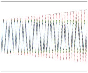
As the simplest case, we begin with the simulation of the first eigen-acoustic mode. As discussed in § 2.2, the transition point of the heater for the first mode is at approximately $l_1=0.43l$ when $\bar {T}_2/\bar {T}_1=1.1$ (refer to figure 6). Therefore, we select three heat positions $l_1/l=0.42,0.433,0.45$, and set $\alpha _1=0.1$, $\omega ={\rm \pi} \bar {c}_1/l$ in the initial heat disturbance (3.11). The initial heater is turned off at $t=T_{eg}$. Then the $n$-$\tau$ flame model is enabled for $Q'(t)$. After $15T_{eg}$, the flow fluctuations reach a fully developed state, and their changes over time are shown in figure 10. It is observed that when $l_1/l=0.42$, the pressure oscillation grows gradually, whereas for $l_1/l=0.44$, the oscillation of pressure attenuates with time. For $l_1/l=0.433$, the amplitude of the pressure fluctuation appears invariant after $t>15T_{eg}$. These phenomena can be demonstrated more clearly in figure 11, where the temporal spectra of $p'(t)$ during $t=15T_{eg}\unicode{x2013} 25T_{eg}$ and $t=25T_{eg}\unicode{x2013} 35T_{eg}$ are illustrated. It is evident that $l_1/l=0.42$ and $l_1/l=0.45$ lead to increment and decrement of $\hat {p}'$, respectively, and the pressure spectrum is nearly unchanged for $l_1/l=0.433$. These observations are consistent with previous LSA predictions in § 2.2.

Figure 10. The LBM simulation of the first oscillation mode with different heater locations in a Rijke tube. Other parameters are $\mbox {Ma}_1=0.01$, $\bar {T}_2=1.1$, $N=3$. The dotted line shows the envelope curve fitted with (3.16), and the fitted coefficients are $p'_0=7.7\times 10^{-5}\bar {\rho }_1\bar {c}^2_1$, $\omega _i=7.7\times 10^{-3}\bar {c}_1/l$.

Figure 11. Pressure oscillation spectra of the fields shown in figure 10 at two time ranges, for: (a) $l_1/l=0.42$, (b) $l_1/l=0.433$, (c) $l_1/l=0.45$.

As a more quantitative study, we examine the detailed growth rate from the LBM result for the first and second modes. For the first mode, in addition to the three cases illustrated in figure 10, two additional cases with $l_1/l=0.41$ and $0.46$ are simulated to verify a wider range. For the second mode, five cases with $0.67\leqslant l_1/l\leqslant 0.72$ are simulated. In each case, the envelope of $p'$ peaks is expected to satisfy

(3.16)\begin{equation} p'(t_m)=p'_0\,\mathrm{e}^{\omega_i t_m} \Rightarrow \ln p'(t_m)=\ln p'_0+\omega_i t_m, \end{equation}

where $t_m$ is the time for $p'$ to reach the $m$th peak value. The actual growth rate $\omega _i$ and fundamental amplitude $p'_0$ can be obtained by least squares fit of (3.16) from a series of $(t_m, p'(t_m))$, as shown in figure 10. The extracted growth rates, as well as the solutions from LSA, are shown in figure 12. It is observed that the growth rates from the two approaches are quite consistent with each other.

Figure 12. The growth rate of $p'$ near the transition point for (a) the first mode and (b) the second mode. Other parameters are $\mbox {Ma}_1=0.01$, $\bar {T}_2=1.1$ and $N=3$.

We further consider the cases with different downstream temperatures $\bar {T}_2$, which essentially means different mean heat release rate $\bar {Q}$. Additionally, we consider four different upstream velocities, $\mbox {Ma}_1=0.01$, 0.1, 0.2 and 0.3. The assembled result is shown in figure 13. It is observed that the growth rate increases with higher downstream temperature $T_2$, which is straightforward since more heat released in the flow makes the system more unstable. On the other hand, the upstream Mach number seems to have a negative effect on the growth rate, i.e. a higher heat release rate (or $\bar {T}_2$) is required to trigger the acoustic wave to increase at higher $Ma_1$. For the same $\bar {T}_2$, flows with lower Mach numbers always exhibit larger growth rates compared to higher $Ma_1$ cases. These results are consistent with the phase diagrams solved with LSA and shown in figure 7, and the reason for the change of growth rate can be explained with the Rayleigh criterion (2.37) as well as the balance of gain and loss of sound energy; see the discussions near figures 7 and 8 for details.

Figure 13. The growth rate of $p'$ for the first mode under different upstream Mach numbers with $N=3.0$ and $l_1/l=1/4$.

For different flame interaction strengths $N=1$, 2 and 3, the growth rates and transition points for $\bar {T}_2$ are also studied with the LBM. The result is shown in figure 14. It is evident that the $\omega _i$ extracted from the simulated flow field closely matches the LSA results. Furthermore, as the interaction strength increases, the $\bar {T}_2$ required for waves to grow decreases rapidly. This can be explained by the heat release perturbation in an FTF as well, that a more sensitive flame is usually more unstable.

Figure 14. The growth rate of $p'$ for the first mode with different $N$ at $\mbox {Ma}_1=0.01$ and $l_1/l=1/4$.

3.4. LBM simulation of thermoacoustic waves with two mixed modes

Previous LBM simulations have focused solely on a single oscillation mode. In this subsection, we consider a more complex situation involving a thermoacoustic field composed by the first and second modes. As discussed above and shown in figure 6(b), the transition point from increment to decay for the first eigenmode is $l_1=0.433$, while the transition point from damping to increasing for the second mode is $l_1\approx 0.5$. Therefore, we expect that when $l_1/l=0.25$, the first mode will grow and the second mode will decay. To observe the evolving process more clearly, we set $\alpha _1=0.01$ and $\alpha _2=0.2$ in (3.11) so that the damping mode is initialized with a larger amplitude and the increasing mode is initialized with a smaller value. We further set $\omega ={\rm \pi} \bar {c}_1/l$ in the initial heat release disturbance (3.11). The initial heater is turned off at $t=T_{eg}$. Then the $n$-$\tau$ flame model is employed for $Q'(t)$. The result for the mixed modes with $l_1/l=0.25$ is shown in figure 15. It is observed that although the second mode (the shorter wave) is dominant at the beginning, it decays gradually over time. At time $t=50T_{eg}$, the shorter wave almost disappears, while the longer wave, i.e. the first mode, becomes predominant in figure 15 and continues to increase over time.

Figure 15. The LBM solution of the mixed acoustic modes. The initial heater coefficients are $\alpha _1=0.01$, $\alpha _2=0.2$. Other parameters are $\mbox {Ma}_1=0.01$, $\bar {T}_2=1.1$, $N=3$ and $l_1/l=1/4$.

In figure 16, the spectra of the pressure oscillations for the two mixed-mode cases in the time intervals $t=10T_{eg}\unicode{x2013} 30T_{eg}$ and $t=30T_{eg}\unicode{x2013} 50T_{eg}$ are illustrated. It is evident that the amplitude of the first mode in the second time interval is lower than at the beginning, while the amplitude of the second mode exhibits the opposite behaviour. This result confirms that mixed modes are also consistent with the stability ranges predicted by LSA.

Figure 16. Spectra of the pressure oscillation for the mixed acoustic modes of figure 15 in two time intervals.

4. Lattice Boltzmann simulation with nonlinear flame model

In previous sections, all the analyses are based on the linear flame model. Results show that the unstable modes will continue to increase indefinitely with the $n$-$\tau$ model given a sufficiently long period, whereas in realistic conditions, the final amplitude remains finite. Consequently, several nonlinear models have been developed to address this issue (Fleifil et al. 1996; Dowling 1997, 1999; Dowling & Stow 2003). In this section, we introduce a modification to the flame model to preserve the developing characteristics of the linear model when the amplitude is small; as the amplitude reaches a predefined value, the system will stabilize, and waves will not amplify further. This approach is to add a piecewise ‘saturation function’ to $Q'(t)$, as proposed by Stow & Dowling (2009), i.e.

(4.1)\begin{equation} Q'(t)= \left\{ \begin{array}{@{}ll} Q'_{L}(t), & | Q'_{L}(t)|<\kappa \bar{Q},\\[2pt] \mathrm{sgn}(Q^{\prime}(t))\,\kappa \bar{Q}, & | Q'_{L}(t)|\geqslant \kappa \bar{Q}, \end{array} \right. \end{equation}

where $\kappa$ is a constant representing the expected saturation extent with $\bar {Q}$, and $Q'_{L}(t)$ represents the linear model part expressed by (2.9). The sign function $\mathrm {sgn}(x)$ is $1$ when $x\geqslant 0$, and returns $-1$ when $x$ is negative. The coefficient $\kappa$ is associated with flame models constructed from the realistic saturation status in combustors (Stow & Dowling 2004; Bellucci et al. 2005), such that $0<\kappa <1$ should be adopted. Here, we choose $\kappa =0.01$ without loss of generality, since the frequencies of thermoacoustic modes are not affected much by the specific value of $\kappa$.

We first consider an initial condition with mixed modes, excited by setting the initial heat release perturbation in (3.11) with $\alpha _1=\alpha _3=0.2$, i.e. the first and third eigenmodes are imposed at the beginning. The result is shown in figure 17. Instead of plotting $p'$, $u'$ is illustrated here since the final amplitude can be compared with the result of limit cycle theory described later. It can be seen from figure 17 that both the shorter and longer waves are significant at the beginning. As time progresses, the oscillation is gradually dominated by the longer wave, i.e. the first mode, while waves of other lengths gradually become invisible. By $t=70T_{eg}$, the velocity fluctuation becomes a periodic wave with constant amplitude. The final amplitude of $u'(t)$ can be determined using the limit cycle theory (Stow & Dowling 2009), which establishes a balance between the velocity fluctuation and energy input for nonlinear flame model; see Appendix D for details. This theory yields the stable velocity fluctuation as $u'\approx 1.85\times 10^{-4}\bar {c}_1$, as shown in figure 17.

Figure 17. The LBM simulation of the velocity oscillation with the nonlinear flame model at $l_1=l/4$. The first and third modes are excited at $t=0\unicode{x2013} 2T_{eg}$. The dashed lines denote the amplitude predicted by the limit cycle theory with $u'\approx 1.85\times 10^{-4}\bar {c}_1$.

The spectra of the velocity perturbation in the time intervals $t=20T_{eg}\unicode{x2013} 45T_{eg}$ and $t=45T_{eg}\unicode{x2013} 70T_{eg}$ are illustrated in figure 18. It can be observed that the first and third modes have almost equivalent energy initially (the third mode diminishes slightly during the developing process), consistent with the initial heat disturbance. In the time interval $t=45T_{eg}\unicode{x2013} 70T_{eg}$, the amplitude of the first mode is approximately double the beginning status, while the third mode decays significantly. An interesting phenomenon is that the third mode cannot be eliminated completely, regardless of how long the simulation runs. For instance, we have run this case to $500T_{eg}$, and the amplitude of the third mode in $t=475T_{eg}\unicode{x2013} 500T_{eg}$ is also shown in figure 18. We can see that $|\hat {u}'|$ for the third mode is almost unchanged after $t>70T_{eg}$. The persistence of the third harmonic wave with low amplitude has also been detected by Stow & Dowling (2009). This occurs because as the system reaches the limit cycle condition, the nonlinear effect of the flame model continues contributing to the energy of the third mode. Eventually, the increasing and damping factors reach an equilibrium, maintaining the presence of the third mode.

Figure 18. Spectra of the velocity oscillation with the nonlinear flame model at $l_1=l/4$ in time intervals $t/T_{eg}=20\unicode{x2013} 45$, $t/T_{eg}=45\unicode{x2013} 70$ and $t/T_{eg}=475\unicode{x2013} 500$.

The saturation character (limit cycle) of the nonlinear model can be verified not only from the increasing side but also from the decaying aspect. We consider two cases with only the first eigenmode, where the initial perturbations are given either a smaller heat disturbance $\alpha _1=0.1$ or a larger value of $\alpha _1=0.4$. The other parameters remain the same as in the previous mixed modes case in this section. Figure 19 shows the temporal evolution of the velocity fluctuations. The results indicate that the acoustic wave with smaller initial amplitude grows rapidly, consistent with the dispersion analysis’ prediction. On the other hand, the oscillation with a larger initial amplitude decays even if it is at the same frequency. This confirms that the saturation factor in (4.1) has taken effect at such a large amplitude. At $t=70T_{eg}$, the acoustic waves of both cases converge to the same state and eventually approach the limit cycle value $u'\approx 1.85\times 10^{-4}\bar {c}_1$.

Figure 19. The LBM simulations of the velocity oscillation with the nonlinear flame model at $l_0=0.25l$ and two initial wave amplitudes. The dashed lines denote the amplitude predicted by the limit cycle theory, with $u'\approx 1.85\times 10^{-4}\bar {c}_1$.

5. Conclusion

In this paper, the influence of the heater position, mean flow, and heat release parameters on the stability of thermoacoustic waves in a one-dimensional Rijke tube is studied, using both classic linear stability analysis (LSA) and the lattice Boltzmann method (LBM). Three types of flame models are proposed to represent the ideal time-lag heat release model, the frequency-selected interaction flame, and the nonlinear flame with both finite frequency and amplitude. The stability ranges for the most simplified system, assuming both zero velocity and small Mach number, can be obtained analytically, while LSA without these simplifications can be solved numerically. We find that the growth rate of a pressure perturbation increases with a higher heat release rate, while it decreases with a higher mean velocity provided that other flow parameters are kept the same. A larger flame interaction strength $N$ in the flame model can increase the growth rate and growing range significantly, while the effect of the lag time $\tau$ on growth rate is periodic due to the Rayleigh criterion.

A multi-speed LBM with a heat source is proposed to address thermoacoustic problems. It is constructed using our recently developed spectral multiple-relaxation-time (SMRT) collision model and characteristic boundary conditions. Then the LBM is implemented with both the linear and nonlinear flame models to validate the LSA predictions. We perform several simulations with the first, second and mixed eigen-acoustic modes. Their developing characteristics and growth rates are consistent with the results from the LSA. The final fluctuation amplitude of the LBM simulation with the nonlinear model coincides with the value obtained by the limit cycle theory.

These results demonstrate the capability of the multi-speed LBM with SMRT model to simulate thermoacoustic problems. The next step is to extend the current analysis and simulation approaches to two- and three-dimensional problems. Meanwhile, a more realistic flame model and complex combustor boundaries should also be adopted. These are currently under active research by the authors, and will be presented in future work.

References

Alexander, F.J., Chen, H., Chen, S. & Doolen, G.D. 1992 Lattice Boltzmann model for compressible fluids. Phys. Rev. A 46 (4), 19671970.CrossRefGoogle ScholarPubMed
Atif, M., Namburi, M. & Ansumali, S. 2018 Higher-order lattice Boltzmann model for thermohydrodynamics. Phys. Rev. E 98, 053311.CrossRefGoogle Scholar
Barad, M.F., Kocheemoolayil, J.G. & Kiris, C.C. 2017 Lattice Boltzmann and Navier–Stokes Cartesian CFD approaches for airframe noise predictions. In 23rd AIAA Comp. Fluid Dyn. Conf. AIAA.CrossRefGoogle Scholar
Bellucci, V., Schuermans, B., Nowak, D., Flohr, P. & Paschereit, C.O. 2005 Thermoacoustic modeling of a gas turbine combustor equipped with acoustic dampers. Trans. ASME J. Turbomach. 127 (2), 372379.CrossRefGoogle Scholar
Benzi, R., Succi, S. & Vergassola, M. 1992 The lattice Boltzmann equation: theory and applications. Phys. Rep. 222 (3), 145197.CrossRefGoogle Scholar
Bloxsidge, G.J., Dowling, A.P. & Langhorne, P.J. 1988 Reheat buzz: an acoustically coupled combustion instability. Part 2. Theory. J. Fluid Mech. 193, 445473.CrossRefGoogle Scholar
Boudy, F., Durox, D., Schuller, T. & Candel, S. 2011 Nonlinear mode triggering in a multiple flame combustor. Proc. Combust. Inst. 33 (1), 11211128.CrossRefGoogle Scholar
Boudy, F., Durox, D., Schuller, T. & Candel, S. 2013 Analysis of limit cycles sustained by two modes in the flame describing function framework. C. R. Méc. 341 (1–2), 181190.CrossRefGoogle Scholar
Buick, J.M., Greated, C.A. & Campbell, D.M. 1998 Lattice BGK simulation of sound waves. Europhys. Lett. 43 (3), 235240.CrossRefGoogle Scholar
Cannon, S.M., Adumitroaie, V. & Smith, C.E. 2001 3D LES modeling of combustion dynamics in lean premixed combustors. In Turbo Expo: Power for Land, Sea, and Air, vol. 78514, V002T02A056. ASME.CrossRefGoogle Scholar
Chen, H., Chen, S. & Matthaeus, W.H. 1992 Recovery of the Navier–Stokes equations using a lattice-gas Boltzmann method. Phys. Rev. A 45 (8), R5339R5342.CrossRefGoogle ScholarPubMed
Chen, S. & Doolen, G.D. 1998 Lattice Boltzmann method for fluid flows. Annu. Rev. Fluid Mech. 30 (1), 329364.CrossRefGoogle Scholar
Chen, X., Yang, K. & Shan, X. 2023 Characteristic boundary condition for multispeed lattice Boltzmann model in acoustic problems. J. Comput. Phys. 490, 112302.CrossRefGoogle Scholar
Chen, Y., Ohashi, H. & Akiyama, M. 1994 Thermal lattice Bhatnagar–Gross–Krook model without nonlinear deviations in macrodynamic equations. Phys. Rev. E 50 (4), 27762783.CrossRefGoogle ScholarPubMed
Crocco, L. 1951 Aspects of combustion stability in liquid propellant rocket motors. Part I. Fundamentals, low frequency instability with monopropellants. J. Am. Rocket Soc. 21 (6), 163178.CrossRefGoogle Scholar
Delgado-Gutierrez, A., Marzocca, P., Cardenas, D. & Probst, O. 2020 A highly accurate GPU lattice Boltzmann method with directional interpolation for the probability distribution functions. Intl J. Numer. Meth. Fluids 92 (12), 17781797.CrossRefGoogle Scholar
Dowling, A.P. 1995 The calculation of thermoacoustic oscillations. J. Sound Vib. 180 (4), 557581.CrossRefGoogle Scholar
Dowling, A.P. 1997 Nonlinear self-excited oscillations of a ducted flame. J. Fluid Mech. 346, 271290.CrossRefGoogle Scholar
Dowling, A.P. 1999 A kinematic model of a ducted flame. J. Fluid Mech. 394, 5172.CrossRefGoogle Scholar
Dowling, A.P. & Stow, S.R. 2003 Acoustic analysis of gas turbine combustors. J. Propul. Power 19 (5), 751764.CrossRefGoogle Scholar
Fleifil, M., Annaswamy, A.M., Ghoneim, Z.A. & Ghoniem, A.F. 1996 Response of a laminar premixed flame to flow oscillations: a kinematic model and thermoacoustic instability results. Combust. Flame 106 (4), 487510.CrossRefGoogle Scholar
Hantschk, C.-C. & Vortmeyer, D. 1999 Numerical simulation of self-excited thermoacoustic instabilities in a Rijke tube. J. Sound Vib. 227 (3), 511522.CrossRefGoogle Scholar
Huang, K. 1987 Statistical Mechanics. John Wiley & Sons.Google Scholar
Hubbard, S. & Dowling, A.P. 2001 Acoustic resonances of an industrial gas turbine combustion system. Trans. ASME J. Engng Gas Turbines Power 123 (4), 766773.CrossRefGoogle Scholar
Kolluru, P.K., Atif, M. & Ansumali, S. 2023 Reduced kinetic model of polyatomic gases. J. Fluid Mech. 963, A7.CrossRefGoogle Scholar
Kuznik, F., Obrecht, C., Rusaouen, G. & Roux, J.-J. 2010 LBM based flow simulation using GPU computing processor. Comput. Math. Appl. 59 (7), 23802392.CrossRefGoogle Scholar
Li, X. & Shan, X. 2021 Rotational symmetry of the multiple-relaxation-time collision model. Phys. Rev. E 103 (4), 043309.CrossRefGoogle ScholarPubMed
Mariappan, S. & Sujith, R.I. 2011 Modelling nonlinear thermoacoustic instability in an electrically heated Rijke tube. J. Fluid Mech. 680, 511533.CrossRefGoogle Scholar
Marié, S., Ricot, D. & Sagaut, P. 2009 Comparison between lattice Boltzmann method and Navier–Stokes high order schemes for computational aeroacoustics. J. Comput. Phys. 228 (4), 10561070.CrossRefGoogle Scholar
Matveev, K.I. 2003 Thermoacoustic Instabilities in the Rijke Tube: Experiments and Modeling. California Institute of Technology.Google Scholar
McNamara, G.R., Garcia, A.L. & Alder, B.J. 1995 Stabilization of thermal lattice Boltzmann models. J. Stat. Phys. 81, 395408.CrossRefGoogle Scholar
Namburi, M., Krithivasan, S. & Ansumali, S. 2016 Crystallographic lattice Boltzmann method. Sci. Rep. 6, 27172.CrossRefGoogle ScholarPubMed
Nie, X., Shan, X. & Chen, H. 2008 a Galilean invariance of lattice Boltzmann models. Europhys. Lett. 81, 34005.CrossRefGoogle Scholar
Nie, X., Shan, X. & Chen, H. 2008 b Thermal lattice Boltzmann model for gases with internal degrees of freedom. Phys. Rev. E 77, 035701.CrossRefGoogle ScholarPubMed
Noiray, N., Durox, D., Schuller, T. & Candel, S. 2008 A unified framework for nonlinear combustion instability analysis based on the flame describing function. J. Fluid Mech. 615, 139167.CrossRefGoogle Scholar
Palies, P., Durox, D., Schuller, T. & Candel, S. 2011 Nonlinear combustion instability analysis based on the flame describing function applied to turbulent premixed swirling flames. Combust. Flame 158 (10), 19801991.CrossRefGoogle Scholar
Pankiewitz, C. & Sattelmayer, T. 2003 Time domain simulation of combustion instabilities in annular combustors. Trans. ASME J. Engng Gas Turbines Power 125 (3), 677685.CrossRefGoogle Scholar
Poinsot, T. 2017 Prediction and control of combustion instabilities in real engines. Proc. Combust. Inst. 36 (1), 128.CrossRefGoogle Scholar
Poinsot, T. & Veynante, D. 2005 Theoretical and Numerical Combustion. R.T. Edwards.Google Scholar
Poinsot, T.J. & Lele, S.K. 1992 Boundary conditions for direct simulations of compressible viscous flows. J. Comput. Phys. 101 (1), 104129.CrossRefGoogle Scholar
Qian, Y.-H., d'Humières, D. & Lallemand, P. 1992 Lattice BGK models for Navier–Stokes equation. Europhys. Lett. 17 (6), 479484.CrossRefGoogle Scholar
Rinaldi, P.R., Dari, E.A., Vénere, M.J. & Clausse, A. 2012 A lattice-Boltzmann solver for 3D fluid simulation on GPU. Simul. Model Pract. Thoery 25, 163171.CrossRefGoogle Scholar
Schuller, T., Poinsot, T. & Candel, S. 2020 Dynamics and control of premixed combustion systems based on flame transfer and describing functions. J. Fluid Mech. 894, P1.CrossRefGoogle Scholar
Shan, X. 2016 The mathematical structure of the lattices of the lattice Boltzmann method. J. Comput. Sci. 17, 475481.CrossRefGoogle Scholar
Shan, X. 2019 Central-moment-based Galilean-invariant multiple-relaxation-time collision model. Phys. Rev. E 100 (4), 043308.CrossRefGoogle ScholarPubMed
Shan, X. & He, X. 1998 Discretization of the velocity space in the solution of the Boltzmann equation. Phys. Rev. Lett. 80 (1), 6568.CrossRefGoogle Scholar
Shan, X., Li, X. & Shi, Y. 2021 A multiple-relaxation-time collision model by Hermite expansion. Phil. Trans. R. Soc. A 379 (2208), 20200406.CrossRefGoogle ScholarPubMed
Shan, X., Yuan, X.-F. & Chen, H. 2006 Kinetic theory representation of hydrodynamics: a way beyond the Navier–Stokes equation. J. Fluid Mech. 550, 413.CrossRefGoogle Scholar
Slimene, S., Yahya, A., Dhahri, H. & Naji, H. 2022 Simulating Rayleigh streaming and heat transfer in a standing-wave thermoacoustic engine via a thermal lattice Boltzmann method. Intl J. Thermophys. 43 (7), 100.CrossRefGoogle Scholar
Stow, S.R. & Dowling, A.P. 2004 Low-order modelling of thermoacoustic limit cycles. In Turbo Expo: Power for Land, Sea, and Air, vol. 41669, pp. 775–786. ASME.CrossRefGoogle Scholar
Stow, S.R. & Dowling, A.P. 2009 A time-domain network model for nonlinear thermoacoustic oscillations. Trans. ASME J. Engng Gas Turbines Power 131 (3), 031502.CrossRefGoogle Scholar
Toffolo, A., Masi, M. & Lazzaretto, A. 2010 Low computational cost CFD analysis of thermoacoustic oscillations. Appl. Therm. Engng 30 (6–7), 544552.CrossRefGoogle Scholar
Urednicek, Z. 2018 Describing functions and prediction of limit cycles. WSEAS Trans. Sys. Cont. 13, 432446.Google Scholar
Wang, X., Shangguan, Y., Onodera, N., Kobayashi, H. & Aoki, T. 2014 Direct numerical simulation and large eddy simulation on a turbulent wall-bounded flow using lattice Boltzmann method and multiple GPUs. Math. Probl. Engng 2014 (1), 742432.Google Scholar
Wang, Y., Sun, D.-K., He, Y.-L. & Tao, W.-Q. 2015 Lattice Boltzmann study on thermoacoustic onset in a Rijke tube. Eur. Phys. J. Plus 130, 110.CrossRefGoogle Scholar
Xi, Y., Li, X., Wang, Y., Xu, B., Wang, N. & Zhao, D. 2022 Experimental study of transition to instability in a Rijke tube with axially distributed heat source. Intl J. Heat Mass Transfer 183, 122157.CrossRefGoogle Scholar