1. Introduction
Solar irradiance measurements performed by Nimbus-7 satellite revealed that the solar constant coherently varied with daily sunspot number (Hickey et al. Reference Hickey, Alton, Kyle and Hoyt1988). This result triggered the idea that the target stars observed in Mount Wilson Observatory HK Project (Wilson Reference Wilson1978; Vaughan, Preston, & Wilson Reference Vaughan, Preston and Wilson1978; Duncan et al. Reference Duncan1991; Baliunas et al. Reference Baliunas1995) could exhibit variability in long-term mean brightness, like observed in their S indexes. Long-term Strömgren photometry in b and y bands were carried out for a sample of target stars of the HK project and a correlation was found between chromospheric and photometric variations, but with a clear diversity between younger and older stars (Lockwood, Skiff, & Radick Reference Lockwood, Skiff and Radick1997, Radick et al. Reference Radick, Lockwood, Skiff and Baliunas1998). Since the main reference is the Sun itself, almost all target stars were chosen as main sequence stars from different spectral types. Baliunas et al. (Reference Baliunas, Nesme-Ribes, Sokoloff and Soon1996) used a sample from HK project targets and discovered a correlation between the cycle length normalised to the rotation period (
![]() $P_{\rm cyc}/P_{\rm rot}$
) and the dynamo number,
$P_{\rm cyc}/P_{\rm rot}$
) and the dynamo number,
![]() $D\sim1/P_{\rm rot}$
, which was expected to provide clues about the type of the dynamo operating in these stars. Further studies on the HK project targets also revealed a linear positive correlation between
$D\sim1/P_{\rm rot}$
, which was expected to provide clues about the type of the dynamo operating in these stars. Further studies on the HK project targets also revealed a linear positive correlation between
![]() $P_{\rm rot}$
and the rotational period variation amplitude
$P_{\rm rot}$
and the rotational period variation amplitude
![]() $\Delta\,P$
(Donahue, Saar, & Baliunas Reference Donahue, Saar and Baliunas1996). Since
$\Delta\,P$
(Donahue, Saar, & Baliunas Reference Donahue, Saar and Baliunas1996). Since
![]() $\Delta\,P$
is commonly accepted as the proxy of the surface differential rotation, the correlation indicates that slow rotators possess stronger surface differential rotation compared to fast rotators.
$\Delta\,P$
is commonly accepted as the proxy of the surface differential rotation, the correlation indicates that slow rotators possess stronger surface differential rotation compared to fast rotators.
In addition to the Strömgren photometry, some other projects on the long-term photometric observations of chromospherically active stars from various luminosity classes have started by different groups (Henry & Eaton 1995; Strassmeier et al. Reference Strassmeier, Boyd, Epand and Granzer1997; Rodonò et al. Reference Rodonò, Cutispoto, Lanza and Messina2001) with automated photoelectric telescopes (APTs). These efforts enabled to trace long-term photometric behaviour of chromospherically active giant and subgiant stars, in addition to the HK project stars.
Efficient and precise broad-band V observations obtained from APTs allowed studying photometric activity cycles for main sequence and giant stars (Oláh & Strassmeier Reference Oláh and Strassmeier2002; Messina & Guinan Reference Messina and Guinan2003; Oláh et al. Reference Oláh, Moór, Strassmeier, Borkovits and Granzer2013). Furthermore, these observations enabled studies on photometric period variations and long-term tracing of the light curve properties of giant and subgiant stars (Jetsu, Henry, & Lehtinen Reference Jetsu, Henry and Lehtinen2017). These studies allowed to make a comparison between photometric properties of the magnetic activity on these stars and the sunspot cycle (see, e.g. Fekel & Henry Reference Fekel and Henry2005; Özdarcan et al. Reference Özdarcan, Evren, Strassmeier, Granzer and Henry2010). For instance, Fekel et al. (Reference Fekel, Henry, Eaton, Sperauskas and Hall2002) analysed long-term photometric data of two SB1 systems, HD 89546 and HD 113816, and did not find any correlation between the photometric period and the mean brightness, which is a typical properties of the sunspot cycle. However, 10 yr later, Özdarcan, Evren, & Henry (Reference Özdarcan, Evren and Henry2012) re-analysed the long-term photometry of HD 89546, which was doubled as the time coverage of the data compared to the former study and showed that the distribution of the mean brightness with respect to the photometric period is similar to the one observed in the sunspot cycle (see Figure 6 in their study). Besides these APT observations, photometric sky surveys, such as The All Sky Automated Survey (ASAS3, Pojmanski Reference Pojmanski1997; Reference Pojmanski2002; Pojmanski, Pilecki, & Szczygiel Reference Pojmanski, Pilecki and Szczygiel2005) and All-Sky Automated Survey for Supernovae Sky Patrol (ASAS-SN, Shappee et al. Reference Shappee2014; Kochanek et al. Reference Kochanek2017) also provided long-term photometric data for a given position on the sky plane, which is also useful for long-term photometric analyses of chromospherically active stars (see, e.g. Özdarcan & Dal Reference Özdarcan and Dal2018). All these studies led to an increase in the number of well-studied giant and subgiant stars, thus reliable statistical evaluation of magnetic activity properties of these stars became possible. Owing to these studies, it came out that both main sequence and giant stars obey the relation between (
![]() $P_{\rm cyc}/P_{\rm rot}$
) and (
$P_{\rm cyc}/P_{\rm rot}$
) and (
![]() $1/P_{\rm rot}$
), without a significant diversity between the luminosity classes (Oláh & Strassmeier Reference Oláh and Strassmeier2002; Oláh et al. Reference Oláh2009). However, giant and subgiant stars still need more attention. We still do not know precisely if the photometric properties of the magnetic activity in these stars are similar or dissimilar to the photometric properties of the solar activity. On the other hand, test bench of the theoretical studies, in the scope of the mean field dynamo models, has not been fulfilled sufficiently for cool giant and subgiant region in the Hertzsprung–Russell diagram.
$1/P_{\rm rot}$
), without a significant diversity between the luminosity classes (Oláh & Strassmeier Reference Oláh and Strassmeier2002; Oláh et al. Reference Oláh2009). However, giant and subgiant stars still need more attention. We still do not know precisely if the photometric properties of the magnetic activity in these stars are similar or dissimilar to the photometric properties of the solar activity. On the other hand, test bench of the theoretical studies, in the scope of the mean field dynamo models, has not been fulfilled sufficiently for cool giant and subgiant region in the Hertzsprung–Russell diagram.
Table 1. Identifiers, J2000 equatorial coordinates, V magnitudes, and the rotation periods (P) of the the target stars. In the last column, the first reference is for V magnitude and the second reference is for the period.
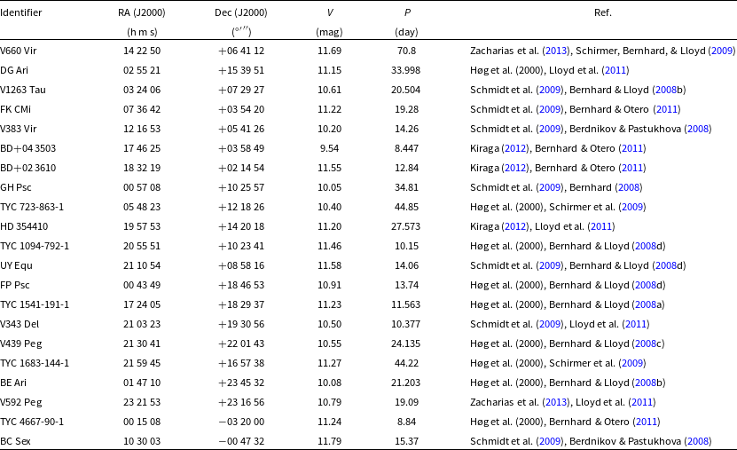
In this study, we present analyses of spectroscopic and long-term photometric observations of 21 stars, which are listed in Table 1 along with their basic properties. These stars were suggested as candidate RS CVn variables in the studies listed in the table. We give technical details of the spectroscopic observations and data reductions in the next section. Then, we focus on spectral types, spectral features in terms of chromospheric activity, and global atmospheric properties of the target stars. In Section 3, we describe sources of the photometric data and analyse long-term brightness variation, together with seasonal light curves. We investigate possible relations between the activity cycle length, the rotation period, and the relative surface shear (i.e. the surface differential rotation) in Section 4. We summarise and discuss our findings in the last section.
2. Spectroscopy
2.1. Data
We obtained intermediate resolution optical échelle spectra of the target stars at TÜBİTAK National Observatory (TNO) with 1.5-m Russian-Turkish telescope and Turkish Faint Object Spectrograph Camera (TFOSCFootnote 1). Until 2017 August 8, optical spectra were recorded by a back illuminated CCD camera with 15 × 15
![]() $\upmu {\rm m}^{2}$
pixel size and 2 048 × 2 048 pixels. After that date, CCD camera was replaced by a new Andor DW436-BV 2 048 × 2 048 pixels CCD camera with a pixel size of 13.5 × 13.5
$\upmu {\rm m}^{2}$
pixel size and 2 048 × 2 048 pixels. After that date, CCD camera was replaced by a new Andor DW436-BV 2 048 × 2 048 pixels CCD camera with a pixel size of 13.5 × 13.5
![]() $\upmu {\rm m}^{2}$
. This instrumental set-up enabled us to record optical spectrum between 3 900 and 9 100 Å in 11 échelle orders with actual spectral resolution (R =
$\upmu {\rm m}^{2}$
. This instrumental set-up enabled us to record optical spectrum between 3 900 and 9 100 Å in 11 échelle orders with actual spectral resolution (R =
![]() $\lambda/\Delta\lambda$
) of 2 700 ± 500 around
$\lambda/\Delta\lambda$
) of 2 700 ± 500 around
![]() $\lambda=5\,500$
Å for both CCD cameras.
$\lambda=5\,500$
Å for both CCD cameras.
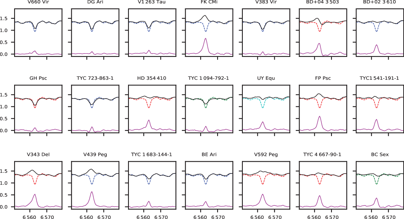
Figure 1. Hαline profiles of the target stars (black lines), comparison stars (dashed lines), and the difference spectrum in the sense of target-minus-comparison (magenta lines). Horizontal and vertical axes show wavelength (Å) and normalised flux, respectively. We shift line profiles of the target and comparison stars upwards by 0.4 in order to see difference spectrum separately. The spectra of comparison stars κ Oph, 35 Peg, o Psc, and ε Psc are in blue, red, green, and cyan colours, respectively.
Raw object spectra were reduced by following conventional échelle reduction steps, starting with bias correction and followed by flat-field division by bias-corrected and normalised flat-field image, scattered light correction, cosmic rays removal, and extraction of the spectra from the échelle orders. Wavelength calibration of the object spectra were done by Fe-Ar calibration lamp spectra. In the final step, extracted and wavelength calibrated object spectra were normalised to the unity order by order, using fourth or fifth order cubic spline functions. All these steps were carried out under IRAF environment.Footnote 2 Since normalisation of spectra is based on fitting a mathematical function to a stellar spectrum, we use these normalised spectra as the initial input for atmosphere analysis. During the atmosphere analysis, these spectra are re-normalised with respect to a proper template synthetic spectrum, which is more reliable for spectrum normalisation.
2.2. Spectral types and features
Beside target stars, we obtained optical échelle spectra of four more stars, κ Oph (K2 III, Gray et al. Reference Gray, Corbally, Garrison, McFadden and Robinson2003), 35 Peg (K0 III, Frasca et al. Reference Frasca, Covino, Spezzi, Alcalá, Marilli, FŻrÉsz and Gandolfi2009), o Psc (G8 III, Jofré et al. Reference JofrÉ, Petrucci, Saffe, Saker, Artur de la Villarmois, Chavero, Gómez and Mauas2015), and ε Psc (G9 III, Soubiran et al. Reference Soubiran, Bienaymé, Mishenina and Kovtyukh2008) with the same instrumental set-up, which are to be used as observational comparison templates. Comparing the template spectra with each of target star spectrum individually, we see that each of the target star spectrum nicely match one of the comparison template spectra, meaning that our sample include only giant and subgiant stars. In Figures 1 and 2, we show Hαand Ca ii H& K line profiles of each target star and the best-matched observational comparison spectrum. These spectral lines are very sensitive to the chromospheric activity observed in cool stars. Some of our target stars exhibit direct emission in Hαline profile, while emission features become visible for other stars in the difference spectrum, in the sense of target-minus-comparison. Emission features are more pronounced in Ca ii H& K line profiles. These line profiles strongly indicate chromospheric activity on these targets. Among our sample, V439 Peg exhibits the strongest emission features both in Hαand Ca ii H& K lines and appears as the most active star in the sample. Another noticeable feature can be seen in Hαline profile of BD+04 3503, which resembles P Cyg line profile. Since the spectral features strongly indicate chromospheric activity, we may speculate that it might be a spectroscopic binary candidate, that one component might be very active and show emission in Hα, while secondary component is a less active or inactive star, thus contributing to composite Hαline profile in form of absorption. Since we only have a single spectrum per target and resolution of TFOSC spectra is limited, it is not possible to detect any shift in spectral lines as an evidence of orbital motion or any spectral line of a possible secondary component.
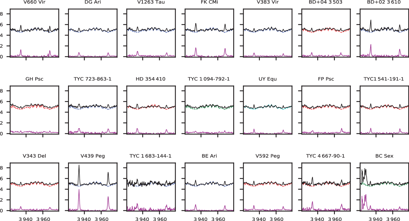
Figure 2. Same as Figure 1 but for Ca ii H& K line profiles. Due to the very strong emission in V439 Peg spectrum, we shift all observed spectra upwards by 4.5, so that emission strength can be seen separately. Note that emission-like feature around 3 925 Å seen in the spectrum of BC Sex is a very strong cosmic spike, which could not be removed properly. However, emission feature of Ca ii K line profile is still visible next to the spike.
2.3. Atmosphere analysis
For further detailed atmospheric analysis of the target stars, we adopt synthetic spectrum fitting method. Main idea of the method is to minimise the difference between the observed and the synthesised spectra for defined wavelength ranges. We apply the method by the newest version of iSpec software (Blanco-Cuaresma et al. Reference Blanco-Cuaresma, Soubiran, Heiter and Jofré2014), which includes various radiative transfer codes, line lists, and model atmospheres in a python framework with a user-friendly graphical user interface. Since each target star appears as a cool giant or subgiant star, we use Turbospectrum (Alvarez & Plez Reference Alvarez and Plez1998; Plez Reference Plez2012) radiative transfer code in conjunction with MARCS model atmospheres (Gustafsson et al. Reference Gustafsson, Edvardsson, Eriksson, Jørgensen, Nordlund and Plez2008). These models are one-dimensional hydrostatic plane-parallel and spherical models computed under local thermodynamic equilibrium (LTE) assumption. In synthetic spectrum fitting and computing, we adopt spherical models, which are more proper for giant stars due to their large radii. Line list compiled from Vienna Atomic Line Database (VALD3, Ryabchikova et al. Reference Ryabchikova, Piskunov, Kurucz, Stempels, Heiter, Pakhomov and Barklem2015) provided by iSpec software is adopted for spectrum synthesising.
For each target star, the first step is to adopt a set of atmospheric parameters estimated in spectrum comparison described in the previous section and synthesise a template spectrum. Then, we shift observed spectrum of the target star to the rest wavelength and re-normalise it with respect to the template. In the normalisation, we adopt the wavelength region between 3 900 and 6 800 Å and compute median for every 5 Å bin within this range for the template spectrum. Computed median values within this wavelength range form a function, which we adopt as the continuum function. Then we divide object spectrum by the continuum function and obtain normalised spectrum of the object. Shifted and re-normalised target spectrum is our input observed data. We set the effective temperature (
![]() $T_{\rm eff}$
), logarithm of the surface gravity (logg), metallicity [(M/H)], micro-turbulence velocity (
$T_{\rm eff}$
), logarithm of the surface gravity (logg), metallicity [(M/H)], micro-turbulence velocity (
![]() $v_{\rm mic}$
), and spectral resolution as adjustable parameters during synthetic spectrum fitting. Considering resolution of TFOSC spectra and reported rotation periods of target stars in Table 1, we neglect line broadening due to projected rotational velocity (
$v_{\rm mic}$
), and spectral resolution as adjustable parameters during synthetic spectrum fitting. Considering resolution of TFOSC spectra and reported rotation periods of target stars in Table 1, we neglect line broadening due to projected rotational velocity (
![]() $v\,\sin\,i$
) and macro-turbulence velocity, that is, fix them to zero. We adopt wavelength range between 4 900 and 6 800 Å for synthetic spectrum fitting but avoid highly blended absorption lines, very strong and broad spectral lines, such as Hαand NaI D resonant lines. We did not extend wavelength range towards bluer part of the spectra since flux of target stars steeply decreases at these wavelengths, leading to considerably lower signal-to-noise ratio. This is natural indication of that we are dealing with cool and red stars. Beyond the 6 800 Å, telluric lines and bands are dominant structures thus we omit this part of the spectrum in atmosphere analysis. When fitting process converges to a solution, we synthesise final template spectrum by adopting solution parameters. Since resolution of TFOSC spectra is not high, it was not necessary to repeat this process iteratively, that is, applying this procedure only for once is fairly enough to achieve an acceptable fit to the observed spectrum and reasonable atmospheric parameters. We tabulate synthetic spectrum fitting results in Table 2.
$v\,\sin\,i$
) and macro-turbulence velocity, that is, fix them to zero. We adopt wavelength range between 4 900 and 6 800 Å for synthetic spectrum fitting but avoid highly blended absorption lines, very strong and broad spectral lines, such as Hαand NaI D resonant lines. We did not extend wavelength range towards bluer part of the spectra since flux of target stars steeply decreases at these wavelengths, leading to considerably lower signal-to-noise ratio. This is natural indication of that we are dealing with cool and red stars. Beyond the 6 800 Å, telluric lines and bands are dominant structures thus we omit this part of the spectrum in atmosphere analysis. When fitting process converges to a solution, we synthesise final template spectrum by adopting solution parameters. Since resolution of TFOSC spectra is not high, it was not necessary to repeat this process iteratively, that is, applying this procedure only for once is fairly enough to achieve an acceptable fit to the observed spectrum and reasonable atmospheric parameters. We tabulate synthetic spectrum fitting results in Table 2.
Table 2. Atmospheric analysis results of target stars. In the last two columns, resolution (
![]() $R=\lambda/\Delta\,\lambda$
) and estimated spectral types of the target stars are given. Spectral type estimation is done by comparing final atmospheric parameters with calibration given in Gray (Reference Gray2005).
$R=\lambda/\Delta\,\lambda$
) and estimated spectral types of the target stars are given. Spectral type estimation is done by comparing final atmospheric parameters with calibration given in Gray (Reference Gray2005).
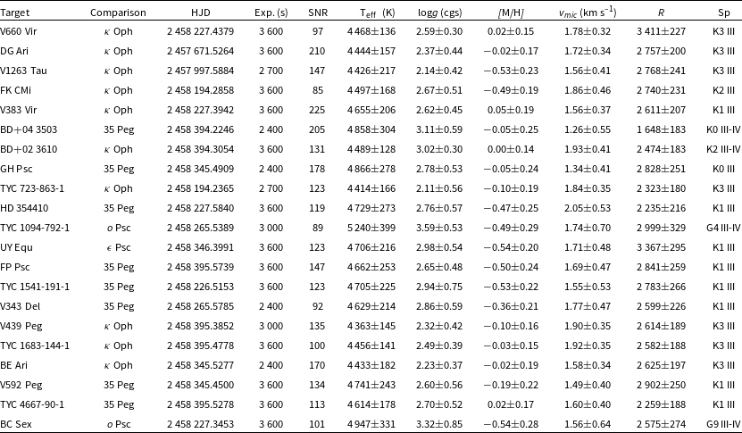
We show observed spectrum of each target with its best-fitting synthetic spectrum in the appendix (Figure A.1). It can be noticed that the spectral lines of BD+04 3503 are shallower and broader compared to the other target stars with similar atmospheric parameters. Furthermore, resulting spectral resolution for this star is considerably lower than the others. These results, together with spectral features of this star reported in Section 2.2, support our speculation on spectroscopic binary possibility. For this star, we repeat synthetic spectrum fitting process with including
![]() $v\,\sin\,i$
as additional adjustable parameters, or neglecting rotational broadening and fixing resolution to different values between 2 200 and 3 300. All these tests result in slightly different atmospheric parameters which basically agree within the uncertainties given in Table 2. We show positions of the target stars on
$v\,\sin\,i$
as additional adjustable parameters, or neglecting rotational broadening and fixing resolution to different values between 2 200 and 3 300. All these tests result in slightly different atmospheric parameters which basically agree within the uncertainties given in Table 2. We show positions of the target stars on
![]() $\log\ T_{\rm eff}-\log\ g$
plane in Figure 3, which clearly shows that our targets are located in giant and subgiant regions in the plane.
$\log\ T_{\rm eff}-\log\ g$
plane in Figure 3, which clearly shows that our targets are located in giant and subgiant regions in the plane.
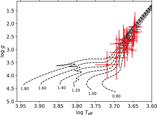
Figure 3. Positions of the target stars on
![]() $\log\ T_{\rm eff}-\log\ g$
plane. Evolutionary tracks are from Bressan et al. (Reference Bressan, Marigo, Girardi, Salasnich, Dal Cero, Rubele and Nanni2012) for
$\log\ T_{\rm eff}-\log\ g$
plane. Evolutionary tracks are from Bressan et al. (Reference Bressan, Marigo, Girardi, Salasnich, Dal Cero, Rubele and Nanni2012) for
![]() $Z=0.014$
and
$Z=0.014$
and
![]() $Y=0.273$
. We also show corresponding mass of each track in unit of the solar mass.
$Y=0.273$
. We also show corresponding mass of each track in unit of the solar mass.
3. Photometry
Long-term V-band photometry of each target star was extracted from The All Sky Automated Survey (ASAS, Pojmanski Reference Pojmanski1997; Pojmanski Reference Pojmanski2002; Pojmanski et al. Reference Pojmanski, Pilecki and Szczygiel2005) and All-Sky Automated Survey for Supernovae Sky Patrol (ASAS-SN, Shappee et al. Reference Shappee2014; Kochanek et al. Reference Kochanek2017) databases. Compiled photometric data from these databases provide observational time base of 16–18 yr, depending on the target. There is a 3- or 4-yr time gap between the last observation of ASAS and the first observation of ASAS-SN data. This gap was filled by ASAS-3N data (Pojmański Reference PojmaŃski2021), which enables us to have continuous V-band photometry of each target without considerable data gap. There are time ranges where data overlap occurs between ASAS and ASAS-3N data. Similar overlap exists for ASAS-3N and ASAS-SN data. These overlaps provide an advantage of comparing different datasets and check for any systematic shift in magnitude axis. ASAS and ASAS-3N data mostly agree, but considerable shifts (maximum 0.m 2) of ASAS-SN data with respect to the ASAS and ASAS-3N data were observed. In such cases, we adopt ASAS data as the reference dataset and apply constant shift in magnitudes with respect to the ASAS data. We do not expect any major effect in cycle search and photometric period analysis results due to such shifts, since we only remove systematic offsets by comparing overlapped data of different datasets.
Before starting analysis, we plot compiled data against time and check for highly deviated observations with respect to the general trend of the whole light curve. The data are mainly used to investigate long-term brightness variation and seasonal photometric behaviour. Therefore, any highly deviated data point, regardless if it shows an instantaneous brightness variation (e.g. flare) or not, were discarded from the dataset. We further check outlier data points in by inspecting phase-folded seasonal light curves. For each seasonal light curve possessing sufficient data points and considerable light curve amplitude, we find a photometric period (see Section 3.2) and compute phase-folded light curve with respect to that period. In order to detect outliers, we fit a cubic spline to the phase-folded light curve, compute residuals from the best-fitting cubic spline and their mean absolute deviation (σ). If any data point is out of
![]() $\pm3\sigma$
band of the residuals, it is removed from the data. Repeating this procedure iteratively until there is no outlier in the corresponding light curve, we obtain final light curves for photometric analysis.
$\pm3\sigma$
band of the residuals, it is removed from the data. Repeating this procedure iteratively until there is no outlier in the corresponding light curve, we obtain final light curves for photometric analysis.
3.1. Mean brightness variations
In the first step of the photometric analysis, we inspect long-term mean brightness variation of each target. For a given target, we first apply linear fit to all data in order to remove any sign of a possible very long-term variation with a timescale much longer than the time base of current photometric data. Then we obtain residuals from the linear fit (hereafter, linear residuals), which scatters around zero level, and search for any long-term periodicities in the linear residuals via Lomb–Scargle periodogram (Lomb Reference Lomb1976; Scargle Reference Scargle1982). Inspecting compiled photometry of target stars given in Figure 4, we did not expect any cyclic variation timescale shorter than 1 year. In order to avoid rotational modulation signal and its harmonics, which could suppress cycle signal in the amplitude spectrum, we did not include periods shorter than 100 d in cycle search. Thus, we scan period range between 100 d and the time span of the compiled photometric data (Δt) given in the last column of the Table 3. We find that 8 of 21 target stars show cyclic mean brightness variation with one significant period. We present compiled photometric data of all target stars and detected mean brightness variations for eight stars in Figure 4 and tabulate detected cyclic variation periods in Table 3. Among remaining 13 targets, 6 of them, DG Ari, V1263 Tau, HD 354410, TYC 1541-191-1, V343 Del, and V592 Peg, only exhibit linear increase or decrease in mean brightness. For the each of remaining seven targets, GH Psc, TYC 723-863-1, TYC 1094-792-1, BC Sex, BE Ari, V439 Peg, and TYC 1683-144-1, we still find statistically significant cycles signal above 3σ threshold, but resulting cycles do not repeat itself more than 1.5 times in the current dataset. Further observations are needed to check the reliability of the detected signals; therefore, we did not consider these stars as cyclic variables and did not include them in Table 3.
Table 3. Cycle period P and amplitude A found in Lomb-Scargle periodogram. In the last column, Δt is the time span of the compiled photometric data.
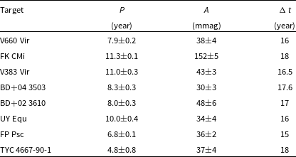
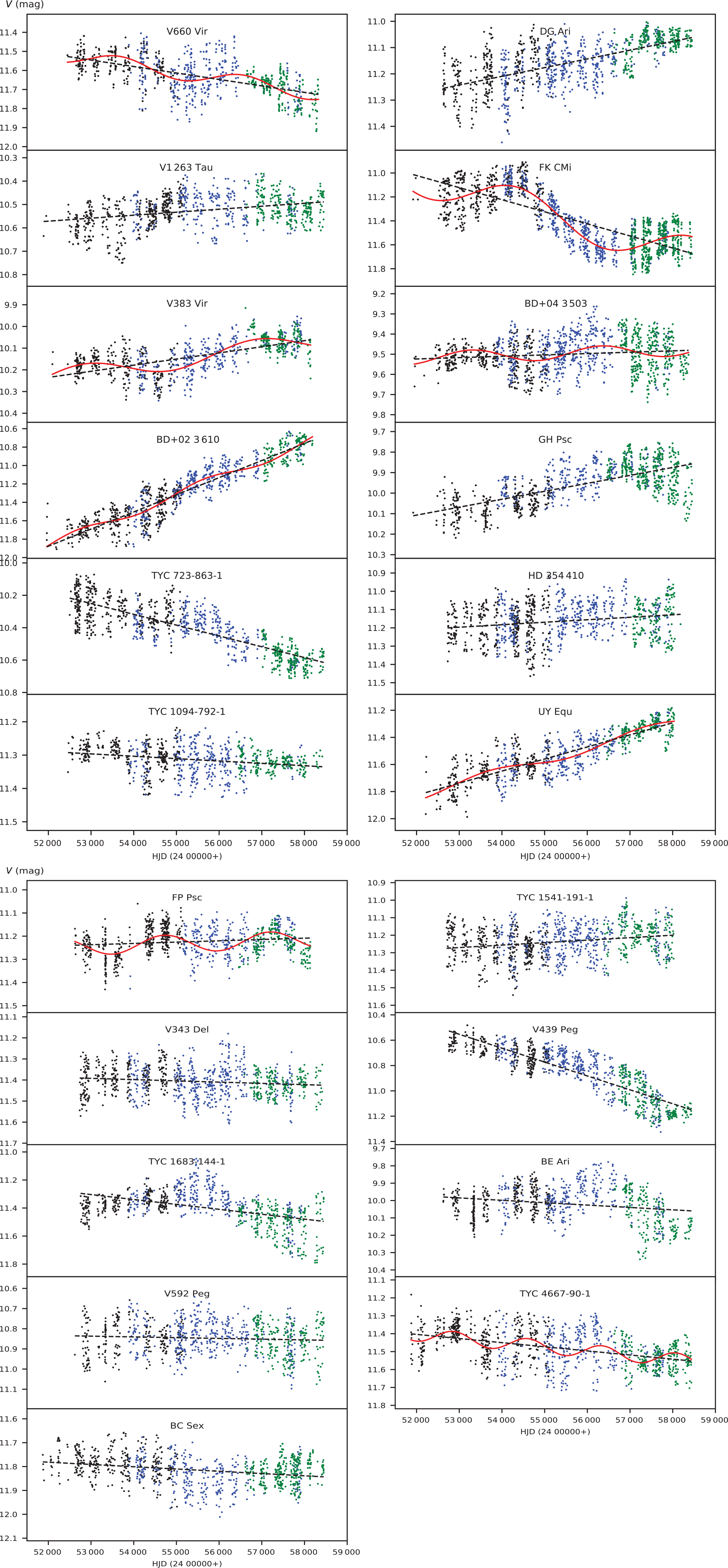
Figure 4. Compiled long-term V-band photometric data of target stars. Black, blue, and green points denote ASAS, ASAS-3N, and ASAS-SN data, respectively. For each star, dashed line shows linear fit to the data. If the target possesses a significant periodic signal, then the signal is shown with continuous (red) curve, which is the combination of periodic signal and linear fit.
We also provide amplitude spectra of the Lomb–Scargle periodogram in Figure B.1, where one may see two peaks above 3σ threshold for some of the target stars. However, these secondary peaks hardly exceed 3σ threshold or vanish below that level after prewhitening of the primary period, therefore did not considered as significant signal.
3.2. Analysis of seasonal light curves
After analysing global brightness variation, we focus on analysis of seasonal light curves of each target. For each seasonal light curve, we try to find photometric period and peak-to-peak light curve amplitude. Inspecting seasonal light curves, we see that light curve shapes are asymmetric or double-humped, which is a typical light curve feature of a chromospherically active star.
Such light curves can be fitted satisfactorily by combining a number of signals with different periods, amplitudes, and phases. One of these signals is the main signal and the remaining signals have periods which are harmonics of the period of the main signal. In this case, one may find many periods, which are statistically significant, for a given single light curve. Our aim is neither make a perfect trigonometric fit to a light curve nor to study harmonics of the main period, but to find a unique period, which represents the light curve as good as possible. Therefore, we adopt ANOVA method (Schwarzenberg-Czerny Reference Schwarzenberg-Czerny1996) which combines strengths of Fourier method and ANOVA statistics. ANOVA method is capable to detect a unique period for an asymmetric or double-humped light curve by evaluating scatter of the phase-folded observational data with respect to a set of trial periods. This method is also very efficient in peak detection and damping alias periods.
We carry out analysis of each target by using the residuals obtained from the linear fit in Section 3.1. The purpose of using the residuals is to reduce unwanted effects of any global (linear) brightening or dimming trend on period and peak-to-peak amplitude detection from seasonal light curves. For each season of each target, we determine start, end, and mean HJD values together with photometric period and its statistical uncertainty, maximum, minimum, and mean brightnesses, peak-to-peak light curve amplitude and number of data points in the season. We tabulate numerical values of these parameters in Table C.1. We adopt the method proposed by Schwarzenberg-Czerny (Reference Schwarzenberg-Czerny1991) to estimate the uncertainty of the seasonal photometric periods. We also compute rotation period of each target by averaging corresponding seasonal photometric periods tabulated in Table C.1. Standard deviation of seasonal photometric periods of each target is adopted as the uncertainty of computed rotation period. Computed rotation periods and uncertainties are listed at the end of Table C.1. Comparing computed rotation periods with the previously reported periods given in Table 1, we see that the computed periods in this study agrees with the previously reported periods in 1σ error bar, except FK CMi and FP Psc. However, for these two stars, difference between previously reported periods and computed periods in this study slightly exceed 1σ error bar.
In the context of solar–stellar connection, one may expect to observe relations between mean brightness, peak-to-peak light curve amplitude, and photometric period. In the Sun, when a new sunspot cycle begins, small sunspots appear at higher latitudes which rotate slower than the solar equator, hence these sunspots have longer rotation periods and causes low-amplitude light loss due to their small size. At the middle of the cycle, sunspots mostly emerge at mid-latitudes with a larger areas and shorter rotation periods compared to the beginning of the cycle. At the end of the cycle, sunspots emerge at lower latitudes with smaller areas and much shorter rotation periods. In summary, photometric period continuously decreases through the cycle while light loss amplitude and mean brightness gradually increase in the first half of the cycle and then gradually decrease towards the end of the cycle.Footnote 3 At that point, we emphasise that the scenario outlined above does not strictly work through the cycle since sunspots could also be emerged at high or low latitudes in the middle of a sunspot cycle. However, these cases do not change the global trends observed in photometric properties.
In order to evaluate each star in the context described above, we present seasonal behaviours of the mean V brightness, peak-to-peak light curve amplitude (A), and photometric period (P) of each target star in Figure 5. Although photometric data spans over 14–18 yr, one may notice some missing seasons in the figure. These missing seasons are due to the sparse data or very low light curve amplitude, which prevent us from finding reliable photometric period and light curve amplitude. Still, we inspect Figure 5, especially for stars exhibiting photometric cycles. For a given target with a cyclic mean brightness variation, general distribution of seasonal photometric periods does not appear coherent with the corresponding cycle and exhibits scattered pattern rather than a systematic decrease trend that repeats itself in each cycle as observed in the sunspot cycle. Regarding light curve amplitude and mean brightness, it is noticeable that the mean brightness tends to increase as the peak-to-peak light curve amplitude decreases.
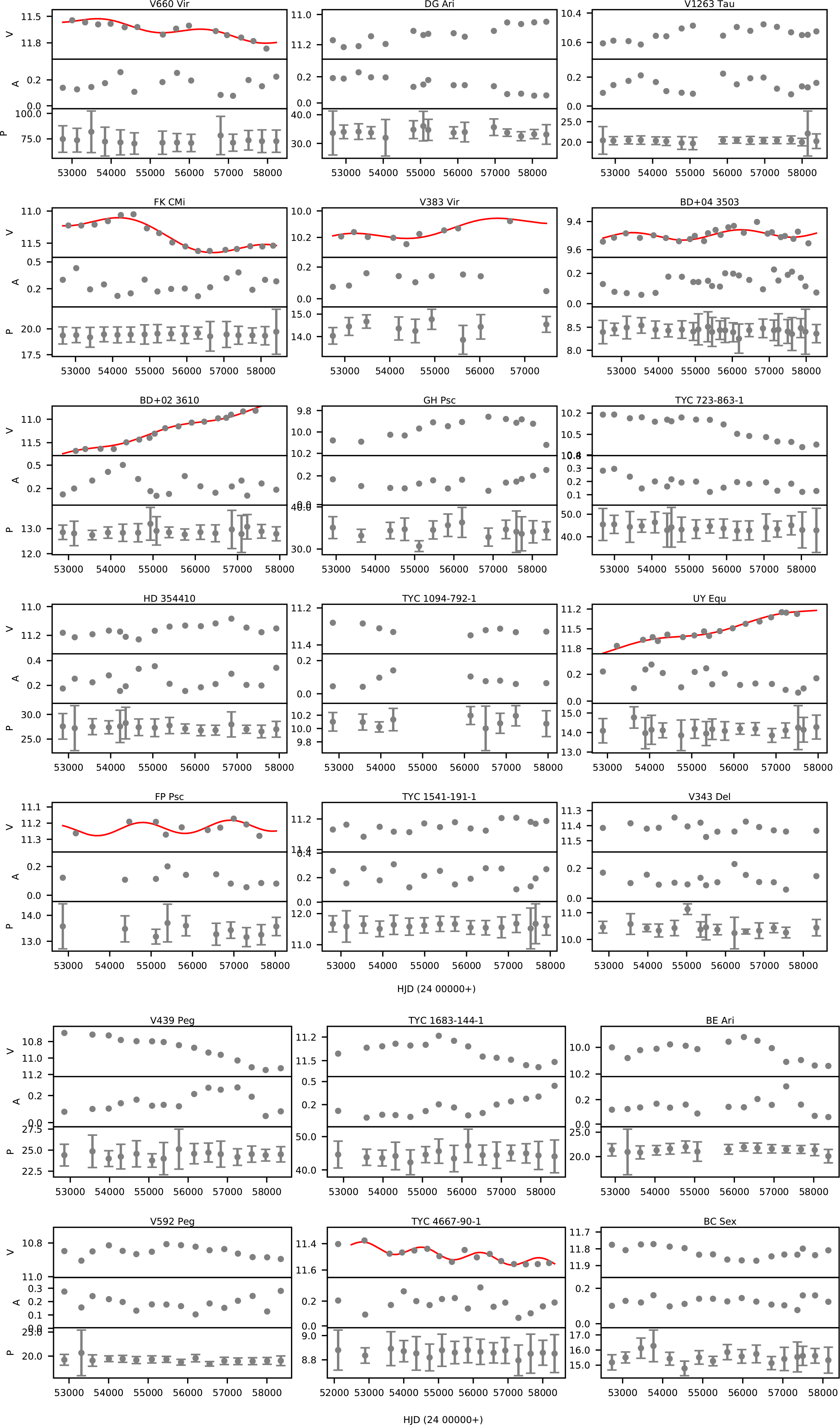
Figure 5. Seasonal mean brightness (V, mag), peak-to-peak light curve amplitude (A, mag), and photometric period (P, day) of each target star are plotted versus time. Detected long-period cycles are overplotted with red continuous line.
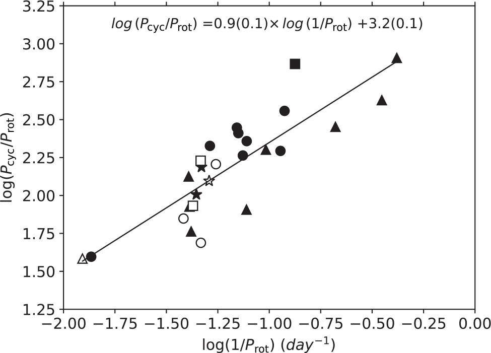
Figure 6. Relation between
![]() $\log(1/P_{\rm rot})$
and
$\log(1/P_{\rm rot})$
and
![]() $\log(P_{\rm cyc}/P_{\rm rot})$
for giant and subgiant stars. Filled circles are stars listed in Table 3, open circles show BD+13 5000, TYC 5163-1764-1 and BD+11 3024 (Özdarcan & Dal Reference Özdarcan and Dal2018), filled stars denote HD 208472 (Özdarcan et al. Reference Özdarcan, Evren, Strassmeier, Granzer and Henry2010) and HD 89546 (Özdarcan et al. Reference Özdarcan, Evren and Henry2012), filled triangles are for IM Peg, HK Lac, XX Tri, IL Hya, HU Vir, UZ Lib, V711 Tau, and FK Com (Oláh et al. Reference Oláh2009), open squares show IS Vir and V2253 Oph (Oláh et al. Reference Oláh, Moór, Strassmeier, Borkovits and Granzer2013) open triangle is BM Cam (Zboril & Messina Reference Zboril and Messina2009), filled square is DM UMa (Taş & Evren Reference Taş and Evren2012), and open star is σ Gem (Kajatkari et al. Reference Kajatkari, Hackman, Jetsu, Lehtinen and Henry2014). Equation of the linear fit is indicated in the insert where numbers in parentheses show statistical errors for the last digit.
$\log(P_{\rm cyc}/P_{\rm rot})$
for giant and subgiant stars. Filled circles are stars listed in Table 3, open circles show BD+13 5000, TYC 5163-1764-1 and BD+11 3024 (Özdarcan & Dal Reference Özdarcan and Dal2018), filled stars denote HD 208472 (Özdarcan et al. Reference Özdarcan, Evren, Strassmeier, Granzer and Henry2010) and HD 89546 (Özdarcan et al. Reference Özdarcan, Evren and Henry2012), filled triangles are for IM Peg, HK Lac, XX Tri, IL Hya, HU Vir, UZ Lib, V711 Tau, and FK Com (Oláh et al. Reference Oláh2009), open squares show IS Vir and V2253 Oph (Oláh et al. Reference Oláh, Moór, Strassmeier, Borkovits and Granzer2013) open triangle is BM Cam (Zboril & Messina Reference Zboril and Messina2009), filled square is DM UMa (Taş & Evren Reference Taş and Evren2012), and open star is σ Gem (Kajatkari et al. Reference Kajatkari, Hackman, Jetsu, Lehtinen and Henry2014). Equation of the linear fit is indicated in the insert where numbers in parentheses show statistical errors for the last digit.
4. Activity cycle length, rotation period, and relative surface shear
We plot target stars listed in Table 3 on
![]() $\log(1/P_{\rm rot})-\log(P_{\rm cyc}/P_{\rm rot})$
plane in Figure 6, where
$\log(1/P_{\rm rot})-\log(P_{\rm cyc}/P_{\rm rot})$
plane in Figure 6, where
![]() $P_{\rm rot}$
is the rotation period in day. We also overplot same values of previously published giant or subgiant stars in the figure. We observe a clear linear trend as reported in previous studies (Baliunas et al. Reference Baliunas, Nesme-Ribes, Sokoloff and Soon1996; Oláh & Strassmeier Reference Oláh and Strassmeier2002; Oláh et al. Reference Oláh2009, Suárez Mascareño, Rebolo, & González Hernández Reference Suárez Mascareño, Rebolo and González Hernández2016); however, we provide quantitative representation of the trend by only using giant and subgiant stars. Linear representation of the data leads to the relation inserted in the figure with a correlation coefficient of 0.85 and probability of no correlation
$P_{\rm rot}$
is the rotation period in day. We also overplot same values of previously published giant or subgiant stars in the figure. We observe a clear linear trend as reported in previous studies (Baliunas et al. Reference Baliunas, Nesme-Ribes, Sokoloff and Soon1996; Oláh & Strassmeier Reference Oláh and Strassmeier2002; Oláh et al. Reference Oláh2009, Suárez Mascareño, Rebolo, & González Hernández Reference Suárez Mascareño, Rebolo and González Hernández2016); however, we provide quantitative representation of the trend by only using giant and subgiant stars. Linear representation of the data leads to the relation inserted in the figure with a correlation coefficient of 0.85 and probability of no correlation
![]() $p=3.5\times10^{-8}$
.
$p=3.5\times10^{-8}$
.
Using maximum and minimum photometric periods of each target tabulated in Table C.1, we compute relative surface shear of each target in terms of
![]() $\Delta\,P/P_{\min}$
. Here,
$\Delta\,P/P_{\min}$
. Here,
![]() $\Delta\,P=P_{\max}-P_{\min}$
, where
$\Delta\,P=P_{\max}-P_{\min}$
, where
![]() $P_{\max}$
and
$P_{\max}$
and
![]() $P_{\min}$
denote maximum and minimum periods, respectively. We plot logarithm of the relative surface shear
$P_{\min}$
denote maximum and minimum periods, respectively. We plot logarithm of the relative surface shear
![]() $\log(\Delta\,P/P_{\min})$
versus
$\log(\Delta\,P/P_{\min})$
versus
![]() $\log(P_{\min})$
in Figure 7 and we find another positive linear correlation with a correlation coefficient of 0.67 and probability of no correlation
$\log(P_{\min})$
in Figure 7 and we find another positive linear correlation with a correlation coefficient of 0.67 and probability of no correlation
![]() $p=1.9\times10^{-4}$
. We also overplot the main sequence stars studied by Donahue et al. (Reference Donahue, Saar and Baliunas1996), who obtained results with a method similar to the one described in our study. Here, we note that we consider minimum periods tabulated in Table 1 of Donahue et al. (Reference Donahue, Saar and Baliunas1996) study and compute
$p=1.9\times10^{-4}$
. We also overplot the main sequence stars studied by Donahue et al. (Reference Donahue, Saar and Baliunas1996), who obtained results with a method similar to the one described in our study. Here, we note that we consider minimum periods tabulated in Table 1 of Donahue et al. (Reference Donahue, Saar and Baliunas1996) study and compute
![]() $\Delta\,P/P_{\min}$
from these data in order to evaluate both datasets properly. Linear regression to the main sequence star data in Figure 7 gives a slope of 0.3, a correlation coefficient of 0.4, and probability of no correlation
$\Delta\,P/P_{\min}$
from these data in order to evaluate both datasets properly. Linear regression to the main sequence star data in Figure 7 gives a slope of 0.3, a correlation coefficient of 0.4, and probability of no correlation
![]() $p=0.014$
. One may easily observe the clear separation of two samples. For a given period, magnitude of the relative surface shear is clearly larger in main sequence stars than giant and subgiant stars. The correlation denotes that the relative surface shear increases with increasing rotational period. Although both samples show positive linear correlations, giant and subgiant sample exhibit linear trend with steeper slope and larger correlation coefficient than the main sequence sample.
$p=0.014$
. One may easily observe the clear separation of two samples. For a given period, magnitude of the relative surface shear is clearly larger in main sequence stars than giant and subgiant stars. The correlation denotes that the relative surface shear increases with increasing rotational period. Although both samples show positive linear correlations, giant and subgiant sample exhibit linear trend with steeper slope and larger correlation coefficient than the main sequence sample.
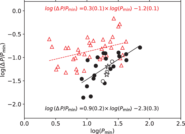
Figure 7. Relation between the minimum rotation period
![]() $P_{\min}$
and the relative surface shear
$P_{\min}$
and the relative surface shear
![]() $\Delta\,P/P_{\min}$
on the logarithmic scale. Filled circles are stars listed in Table 3, open circles show BD+13 5000, TYC 5163-1764-1, and BD+11 3024 (Özdarcan & Dal Reference Özdarcan and Dal2018), open stars denote HD 208472 (Özdarcan et al. Reference Özdarcan, Evren, Strassmeier, Granzer and Henry2010) and HD 89546 (Özdarcan et al. Reference Özdarcan, Evren and Henry2012). Equation of the linear fit (black continuous line) is indicated in the insert (bottom). Open red triangles show stars taken from Donahue et al. (Reference Donahue, Saar and Baliunas1996) and the linear representation of their distribution is shown by red dashed line and given in the insert (top).
$\Delta\,P/P_{\min}$
on the logarithmic scale. Filled circles are stars listed in Table 3, open circles show BD+13 5000, TYC 5163-1764-1, and BD+11 3024 (Özdarcan & Dal Reference Özdarcan and Dal2018), open stars denote HD 208472 (Özdarcan et al. Reference Özdarcan, Evren, Strassmeier, Granzer and Henry2010) and HD 89546 (Özdarcan et al. Reference Özdarcan, Evren and Henry2012). Equation of the linear fit (black continuous line) is indicated in the insert (bottom). Open red triangles show stars taken from Donahue et al. (Reference Donahue, Saar and Baliunas1996) and the linear representation of their distribution is shown by red dashed line and given in the insert (top).
We also inspect possible relation between the activity cycle length and the relative surface shear in Figure 8. Distribution of the data practically indicates no correlation between the cycle length and the relative surface shear.
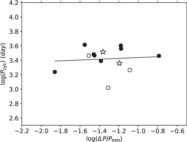
Figure 8. Relation between the activity cycle length and the relative surface shear on the logarithmic scale. The symbols have the same meaning as in Figure 7.
5. Summary and discussion
We present analysis of medium resolution optical spectra and long-term V-band photometry of 21 cool stars. All stars exhibit direct emission features in Ca ii H& K line profiles, while we observe both filled emission and direct emission in Hαlines. Emission features in these spectral lines are clear evidences of chromospheric activity on the target stars. LTE spectrum synthesis shows that the target stars are cool red giant or subgiant stars with an overall metallicity, [M/H], between 0 and
![]() $-0.5$
.
$-0.5$
.
Analysis of long-term V-band photometry of target stars reveals that DG Ari, V1263 Tau, HD 354410, TYC 1541-191-1, V343 Del, and V592 Peg undergo linear mean brightness variation, which may indicate activity cycles in very long timescales. We detect single significant period for eight of the target stars, V660 Vir, FK CMi, V383 Vir, BD+04 3503, BD+02 3610, UY Equ, FP Psc, and TYC 4667-90-1. For each target, resulting cycle signal is superimposed on a linear brightening or dimming trend. Linear trend might show a part of a possible second cycle with a much longer timescale compared to the current dataset. In other words, these stars might possess multiple cycles. Remaining target stars appear to possess photometric cycles, but time base of the current data is not sufficient to confirm these cycles. Possible long-term cycles can be checked only with further V-band observations. Here, we also stress that the cycle periods found in our analysis may only be average values. In case of the sunspot cycle, one can only give an average 11 yr of period, which actually varies between 9 and 14 yr. Therefore, in the context of solar–stellar connection, it is not reasonable to accept strict period values in case of stellar magnetic activity cycles. Oláh, Kolláth, & Strassmeier (Reference Oláh, Kolláth and Strassmeier2000), and Oláh et al. (Reference Oláh2009) clearly showed that photometric cycle periods of cool active stars are variable.
Further analysis of long-term photometric data in terms of seasonal light curve analysis yield photometric period, peak-to-peak light curve amplitude, minimum, maximum, and mean brightnesses of each observing season. For a given target, we compute average value of the seasonal photometric periods and adopt it as the photometric rotation period,
![]() $P_{\rm rot}$
, of the target. Then, we inspect the relation between
$P_{\rm rot}$
, of the target. Then, we inspect the relation between
![]() $\log(1/P_{\rm rot})$
and
$\log(1/P_{\rm rot})$
and
![]() $\log(P_{\rm cyc}/P_{\rm rot})$
of giant and subgiant stars. We observe clear linear trend on the logarithmic scale with a slope of
$\log(P_{\rm cyc}/P_{\rm rot})$
of giant and subgiant stars. We observe clear linear trend on the logarithmic scale with a slope of
![]() $0.9\pm0.1$
, which is consistent with that derived by the slope reported by Oláh et al. (Reference Oláh2009,
$0.9\pm0.1$
, which is consistent with that derived by the slope reported by Oláh et al. (Reference Oláh2009,
![]() $0.81\pm0.05$
) within 1σ level but is considerably higher than the slope reported by Baliunas et al. (Reference Baliunas, Nesme-Ribes, Sokoloff and Soon1996, 0.74), who originally tested the equivalency of the stellar dynamo number (
$0.81\pm0.05$
) within 1σ level but is considerably higher than the slope reported by Baliunas et al. (Reference Baliunas, Nesme-Ribes, Sokoloff and Soon1996, 0.74), who originally tested the equivalency of the stellar dynamo number (
![]() $D\sim1/P_{\rm rot}$
) and
$D\sim1/P_{\rm rot}$
) and
![]() $P_{\rm cyc}/P_{\rm rot}$
ratio. We note that our sample includes only giant and subgiant stars, while Oláh et al. (Reference Oláh2009) used a homogeneous sample, including main sequence and giant stars. If we do not consider the giant stars taken from their study, the slope of the linear fit in Figure 6 increases to
$P_{\rm cyc}/P_{\rm rot}$
ratio. We note that our sample includes only giant and subgiant stars, while Oláh et al. (Reference Oláh2009) used a homogeneous sample, including main sequence and giant stars. If we do not consider the giant stars taken from their study, the slope of the linear fit in Figure 6 increases to
![]() $1.0\pm0.2$
. In any case, these slopes are considerably smaller than the one found in theoretical computations of Dubé & Charbonneau (Reference Dubé and Charbonneau2013, 1.47), who mentioned that the observed linear relation is the robust property of kinematic mean field
$1.0\pm0.2$
. In any case, these slopes are considerably smaller than the one found in theoretical computations of Dubé & Charbonneau (Reference Dubé and Charbonneau2013, 1.47), who mentioned that the observed linear relation is the robust property of kinematic mean field
![]() $\alpha\Omega$
dynamo models with α quenching. Our results support this picture since the activity cycle length is weakly anti-correlated with the relative surface shear, indicating that the activity cycle should be mainly driven by turbulent diffusivity, rather than the differential rotation as anticipated in non-linearly saturated dynamo models. However, although activity cycle length does not appear sensitive to the rotation period for our sample (see Figure 6), longer period stars still tends to have longer period activity cycles, which contradicts with the prediction given by Dubé & Charbonneau (Reference Dubé and Charbonneau2013).
$\alpha\Omega$
dynamo models with α quenching. Our results support this picture since the activity cycle length is weakly anti-correlated with the relative surface shear, indicating that the activity cycle should be mainly driven by turbulent diffusivity, rather than the differential rotation as anticipated in non-linearly saturated dynamo models. However, although activity cycle length does not appear sensitive to the rotation period for our sample (see Figure 6), longer period stars still tends to have longer period activity cycles, which contradicts with the prediction given by Dubé & Charbonneau (Reference Dubé and Charbonneau2013).
Assuming that the
![]() $P_{\min}$
corresponds to the equatorial rotation period, we find that the relative surface shear,
$P_{\min}$
corresponds to the equatorial rotation period, we find that the relative surface shear,
![]() $\Delta\,P/P_{\min}$
, is positively correlated with the equatorial rotation period, which means differential rotation tends to be stronger for slow rotators. Reinhold & Gizon (Reference Reinhold and Gizon2015) made photometric analysis of 12 319 Kepler stars, which are homogeneously distributed in temperature and luminosity class and found that the positive correlation between
$\Delta\,P/P_{\min}$
, is positively correlated with the equatorial rotation period, which means differential rotation tends to be stronger for slow rotators. Reinhold & Gizon (Reference Reinhold and Gizon2015) made photometric analysis of 12 319 Kepler stars, which are homogeneously distributed in temperature and luminosity class and found that the positive correlation between
![]() $P_{\min}$
and the differential rotation exists for stars cooler than 6 000 K. At that point, our study provides quantitative description of the relation for cool giants and subgiant. Moreover, overplotting main sequence stars from the study of Donahue et al. (Reference Donahue, Saar and Baliunas1996) in Figure 7, we observe the clear separation between two samples and more steep slope for giant and subgiant stars. The separation becomes more remarkable towards the shorter periods. Considering evolutionary properties of two samples, we may conclude that the relative surface shear is more sensitive to the rotation period in giant and subgiant stars compared to the main sequence stars. However, magnitude of the relative surface shear for a given period is larger for main sequence stars than giant and subgiant stars. This observational finding appear contradictory to the theoretical model predictions given in Kitchatinov & Rüdiger (Reference Kitchatinov and Rüdiger1999). On the other hand, Kövári et al. (Reference Kövári, Oláh, Kriskovics, Vida, Forgács-Dajka and Strassmeier2017) studied the rotation and the differential rotation relationship via a homogeneous sample in luminosity class whose differential rotation parameters were obtained from Doppler imaging studies. They find a correlation similar to the one shown in Figure 7 but also noticed a distinction between single and binary stars, where the relative surface shear in single stars shows stronger dependency on the rotation period compared to the close binaries. It could be speculated that the separation observed in Figure 7 might be partly caused by being single or binary star. Nevertheless, this needs to be checked by high-resolution spectroscopy for all stars plotted in the figure.
$P_{\min}$
and the differential rotation exists for stars cooler than 6 000 K. At that point, our study provides quantitative description of the relation for cool giants and subgiant. Moreover, overplotting main sequence stars from the study of Donahue et al. (Reference Donahue, Saar and Baliunas1996) in Figure 7, we observe the clear separation between two samples and more steep slope for giant and subgiant stars. The separation becomes more remarkable towards the shorter periods. Considering evolutionary properties of two samples, we may conclude that the relative surface shear is more sensitive to the rotation period in giant and subgiant stars compared to the main sequence stars. However, magnitude of the relative surface shear for a given period is larger for main sequence stars than giant and subgiant stars. This observational finding appear contradictory to the theoretical model predictions given in Kitchatinov & Rüdiger (Reference Kitchatinov and Rüdiger1999). On the other hand, Kövári et al. (Reference Kövári, Oláh, Kriskovics, Vida, Forgács-Dajka and Strassmeier2017) studied the rotation and the differential rotation relationship via a homogeneous sample in luminosity class whose differential rotation parameters were obtained from Doppler imaging studies. They find a correlation similar to the one shown in Figure 7 but also noticed a distinction between single and binary stars, where the relative surface shear in single stars shows stronger dependency on the rotation period compared to the close binaries. It could be speculated that the separation observed in Figure 7 might be partly caused by being single or binary star. Nevertheless, this needs to be checked by high-resolution spectroscopy for all stars plotted in the figure.
Further analyses of individual targets indicate that temporal behaviour of the photometric period does not appear analogous to solar cycle and we do not observe any significant relation between photometric period, mean brightness, and light curve amplitude. We can only say that the mean brightness generally tends to increase as the peak-to-peak light curve amplitude decreases. One may conclude that photometric cycle properties of target stars are not similar to the photometric properties of the sunspot cycle. However, as mentioned in Fekel et al. (Reference Fekel, Henry, Eaton, Sperauskas and Hall2002), the observed photometric period could be affected by the growth and decay of spots or spot groups at various latitudes and longitudes, which means the observed photometric period may not be adopted as a true period of any stellar latitude. Therefore, observed temporal distributions of photometric periods in Figure 5 might partly originate from spot growth and decay. With the current data, it is not possible to arrive at a conclusive result. Further regular V band photometric observations should be continued for successive cycles, so that global photometric behaviour could show itself more clearly in longer timescales. That was the case for HD 89546, where 11 yr of observations did not yield any significant correlation between the photometric period and the mean brightness (Fekel et al. Reference Fekel, Henry, Eaton, Sperauskas and Hall2002), but doubling the time base of the photometric data yielded the correlation (Özdarcan et al. Reference Özdarcan, Evren and Henry2012). Another possibility is that the distribution of the photometric period might be related to a possible cycle which has a timescale longer than the current time base of the photometric data. Observed linear trends in the mean brightness of our target stars might indicate such longer-term cycles. Consequently, we may observe only a part of the whole photometric period variation pattern, which appears as a scatter.
Acknowledgements
I am indebted to Dr. Grzegorz Pojmański for reducing and providing unpublished ASAS-3N data, which compensate long data gap between published ASAS3 and ASAS-SN data and increase the precision of the main results of this study. I also express my thanks to Dr. Hasan Ali Dal for fruitful discussion on statistical analyses. I acknowledge the anonymous referee for his/her helpful comments and valuable suggestions that have significantly contributed to improve the paper. I further thank TÜBİTAK National Observatory for a partial support in using RTT150 (Russian-Turkish 1.5-m telescope in Antalya) with project numbers 14BRTT150-678 and 18BRTT150-1275. This research has made use of the SIMBAD database, operated at CDS, Strasbourg, France. This research received no specific grant from any funding agency, commercial, or not-for-profit sectors.
A. Observed and the best-fitting synthetic spectra
We present plots of observed and the best-fitting synthetic spectrum for each target star separately in Figure A.1.
B. Lomb–Scargle amplitude spectra
We present Lomb–Scargle amplitude spectra of the stars with cyclic mean brightness variation shown in Figure 4.
C. Seasonal photometric analysis of target stars
We tabulate seasonal photometric analysis results in Table C.1.

Figure A.1. Representative plots of atmospheric analysis results for target stars. Observed (black) and best-fitting (red) synthetic spectra together with residuals (blue) are shown for three regions in three windows one under the other.
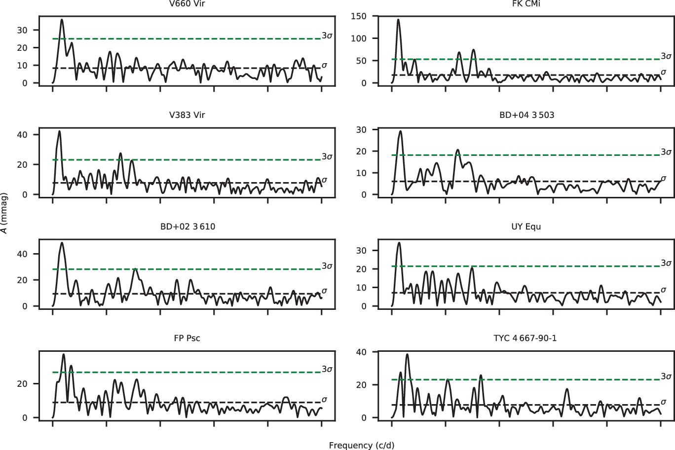
Figure B.1 Lomb–Scargle amplitude spectra of the stars with detected cycle frequencies. Horizontal dashed lines show 1σ and 3σ uncertainty levels. 1σ level is the mean of the amplitude spectrum, which is computed by excluding the dominant peak and its close vicinity.
Table C.1 Photometric analysis results of seasonal light curves. Columns are start, end, and mean HJD of the corresponding light curve, time span of the dataset (Δt), computed photometric period (P) and its uncertainty, maximum, minimum, and mean brightnesses, peak-to-peak amplitude of the light curve (A), and number of data points in the light curve (N). We list computed average photometric period (
![]() $P_{\rm rot}$
) of each target as two columns list at the end of the table. Uncertainty of
$P_{\rm rot}$
) of each target as two columns list at the end of the table. Uncertainty of
![]() $P_{\rm rot}$
is computed via standard deviation of seasonal photometric periods.
$P_{\rm rot}$
is computed via standard deviation of seasonal photometric periods.


