Hostname: page-component-78c5997874-t5tsf Total loading time: 0 Render date: 2024-11-10T19:25:35.040Z Has data issue: false hasContentIssue false

Mixing and inter-scale energy transfer in Richtmyer–Meshkov turbulence

Published online by Cambridge University Press:  08 April 2024

Zhangbo Zhou
Affiliation:
Advanced Propulsion Laboratory, Department of Modern Mechanics, University of Science and Technology of China, Hefei 230026, PR China
Juchun Ding*
Affiliation:
Advanced Propulsion Laboratory, Department of Modern Mechanics, University of Science and Technology of China, Hefei 230026, PR China
Wan Cheng
Affiliation:
Advanced Propulsion Laboratory, Department of Modern Mechanics, University of Science and Technology of China, Hefei 230026, PR China
*
Email address for correspondence: djc@ustc.edu.cn

Abstract

This work investigates the compressible turbulence induced by Richtmyer–Meshkov (RM) instability using high-resolution Navier–Stokes simulations. Special attention is paid to the characteristics of RM turbulence including the mixing width growth, the turbulent kinetic energy (TKE) decay, the mixing degree, inhomogeneity and anisotropy. Three distinct initial perturbation spectra are designed at the interface to reveal the initial condition imprint on the RM turbulence. Results show that cases with initial large-scale perturbations present a stronger imprint on statistical characteristics and also a quicker growth of mixing width, whereas cases with small-scale perturbations present a faster TKE decay, greater mixing level, higher isotropy and homogeneity. A thorough analysis on the inter-scale energy transfer in RM turbulence is also presented with the coarse-graining approach that exposes the two subfilter-scale (SFS) energy fluxes (i.e. deformation work and baropycnal work). A strong correlation between the nonlinear model of baropycnal work (Fluids, 4(2), 2019) and the simulation results is confirmed for the first time, demonstrating its potential in modelling the RM turbulence. Two primary mechanisms of baropycnal work (the straining and baroclinic generation processes) are explored with this nonlinear model. The evolutions of two SFS energy fluxes exhibit distinct behaviours at various filter scales, in different flow regions and under various flow motions (strain and rotation). It is found that all three cases share the common inter-scale energy transfer dynamics, which is important for modelling the RM turbulence.

Type
JFM Papers
Copyright
© The Author(s), 2024. Published by Cambridge University Press

1. Introduction

The Richtmyer–Meshkov (RM) instability (Richtmyer Reference Richtmyer1960; Meshkov Reference Meshkov1969) occurs when a perturbed interface separating two different fluids is subject to an impulsive acceleration typically by a shock wave. After the shock impact, initial perturbations at the interface grow persistently with time and later secondary instabilities such as Kelvin–Helmholtz (KH) instability begin to play a role, potentially leading to a flow transition to turbulent mixing (called RM turbulence). The RM turbulence plays a crucial role in various engineering applications (e.g. inertial confinement fusion [ICF]) and natural phenomena (e.g. supernova explosion). For example, in ICF, the intensive mixing between the inner hot spot and the outer ablator caused by RM instability greatly reduces the energy yield and even causes the ignition failure (Lindl Reference Lindl1995; Lindl et al. Reference Lindl, Amendt, Berger, Glendinning, Glenzer, Haan, Kauffman, Landen and Suter2004; Casner Reference Casner2021; Do et al. Reference Do, Angulo, Nagel, Hall, Bradley, Hsing, Pickworth, Izumi, Robey and Zhou2022). In a scramjet, the mixing between fuel and air enhanced by the RM turbulence could increase the combustion efficiency (Yang, Kubota & Zukoski Reference Yang, Kubota and Zukoski1993; Yang, Chang & Bao Reference Yang, Chang and Bao2014; Ren et al. Reference Ren, Wang, Xiang, Zhao and Zheng2019). The RM turbulence is also a crucial element that should be considered when explaining the supernova remnants (Kifonidis et al. Reference Kifonidis, Plewa, Scheck, Janka and Müller2006; Müller Reference Müller2020). In addition, as a typical variable-density turbulence (Livescu Reference Livescu2020), the RM turbulence that arises from finite, impulsive, directional energy injection, presents unique characteristics differing from other types of turbulence. Hence, the study on RM turbulence constitutes a significant complement to the fundamental research of turbulence (Olmstead et al. Reference Olmstead, Wayne, Simons, Trueba Monje, Yoo, Kumar, Truman and Vorobieff2017).

An important finding in RM turbulence is the discovery of a self-similar stage beyond which the width of the mixing layer exhibits exponential growth with time ($W\propto t^{\theta }$). Numerous studies have been performed to estimate the asymptotic value of the growth exponent $\theta$ (Youngs Reference Youngs2004; Thornber et al. Reference Thornber, Drikakis, Youngs and Williams2010, Reference Thornber2017), which was found to vary in a wide range (0.213, 2/3). A comprehensive summary of the findings on $\theta$ is available in the review of Zhou (Reference Zhou2017a,Reference Zhoub). The various values of $\theta$ obtained indicate the evident influence of initial conditions on the RM turbulence. Previous studies have shown that the initial conditions, especially the initial perturbation spectrum, have a dramatic influence on both the early stage instability evolution and the late-stage turbulent mixing development (Brouillette Reference Brouillette2002; Mikaelian Reference Mikaelian2005; Groom & Thornber Reference Groom and Thornber2020). Such an influence can be elucidated by several potential mechanisms, which are generally divided into two categories (Soulard & Griffond Reference Soulard and Griffond2022): structural and statistical. The former comprises a ‘bubble competition’ mechanism that is initiated by a large-scale perturbation, and a ‘bubble merging’ mechanism (mode coupling of short-wavelength perturbations) that is less sensitive to initial conditions (Elbaz & Shvarts Reference Elbaz and Shvarts2018). The latter incorporates theoretical insights from homogeneous isotropic turbulence into the context of RM turbulence, which arises from the persistence of large eddies (Chasnov Reference Chasnov1997; Llor Reference Llor2006; Soulard et al. Reference Soulard, Guillois, Griffond, Sabelnikov and Simoëns2018). Previous studies have provided a preliminary understanding of the influence of initial conditions on the mixing zone growth. In this work, we intend to conduct a comprehensive and in-depth analysis on the influences of initial perturbation spectrum on the RM turbulence in various aspects, including turbulent kinetic energy (TKE), mixing degree, inhomogeneity and anisotropy, aiming to attain a thorough understanding of initial condition influences.

The study of inter-scale energy transfer is an effective means to gain insights into turbulence. From the perspective of energy cascade, energy is injected at large scales, then transferred progressively to smaller scales and dissipated ultimately into heat at the Kolmogorov scale. An example is the three-dimensional (3-D) Taylor–Green vortex problem (Taylor & Green Reference Taylor and Green1937; Brachet et al. Reference Brachet, Meiron, Orszag, Nickel, Morf and Frisch1983), where turbulence is generated as large vortex roll-ups break down and later small eddies take over the flow field, causing turbulent decay. Although the classical energy cascade process seems simple and clear, the underlying physical mechanisms remain ambiguous (Alexakis & Biferale Reference Alexakis and Biferale2018). Existing studies on the energy cascade focused mainly on incompressible flows (Eyink Reference Eyink2005; Domaradzki, Teaca & Carati Reference Domaradzki, Teaca and Carati2009; Eyink & Aluie Reference Eyink and Aluie2009), in which the sole pathway for inter-scale energy transfer is deformation work. For instance, McKeown et al. (Reference McKeown, Ostilla-Mónico, Pumir, Brenner and Rubinstein2020) studied the vortex ring collision both experimentally and numerically, and found the evidence that links the cascade process with vortex interactions (i.e. deformation). It was found that there are other pathways for the inter-scale energy transfer in compressible or variable-density turbulence (Aluie Reference Aluie2011, Reference Aluie2013; Wang et al. Reference Wang, Yang, Shi, Xiao, He and Chen2013), namely baropycnal work, $\varLambda _{\ell } = \partial _j\bar {p}\bar {\tau }(\rho,u_j)/\bar {\rho }$. Baropycnal work results from the variations in pressure and density, making it sensitive to density and pressure gradients. This phenomenon can occur in both barotropic and baroclinic cases, since it can be non-zero when pressure and density gradients are either aligned or misaligned. Recently, the study of energy transfer between scales through filtering methods has been applied to the Rayleigh–Taylor (RT) (Rayleigh Reference Rayleigh1883; Taylor Reference Taylor1950) turbulence. For instance, Zhou et al. (Reference Zhou, Huang, Lu, Liu and Ni2016) examined the inter-scale transfer of kinetic energy, thermal energy, and enstrophy in two-dimensional (2-D) Boussinesq RT turbulence. It was found that on average, kinetic energy undergoes a dynamic transfer from small to large scales through an inverse cascade, whereas both thermal energy and enstrophy are transferred towards small scales through forward cascades. Zhao, Liu & Lu (Reference Zhao, Liu and Lu2020) examined the inter-scale transfer of kinetic energy and enstrophy in 3-D compressible RT turbulence. It was found that kinetic energy can transfer between scales through both deformation work and baropycnal work. The former is responsible for transferring kinetic energy at small scales, whereas the latter is responsible for transferring kinetic energy at large scales. Recently, Zhao, Betti & Aluie (Reference Zhao, Betti and Aluie2022) compared the energy scale transfer in 2-D and 3-D RT turbulence, and found that the baropycnal work serves as a conduit for the continuous non-local transfer of potential energy from the largest scale to smaller scales within the inertial region, in which the cascade process is dominated by deformation work.

Unlike the RT turbulence, in which potential energy is transformed continuously into kinetic energy, RM turbulence generates kinetic energy solely during the interaction of the shock with the interface. The gradual transfer of kinetic energy that shares the same scales as initial perturbations to other generative scales is a crucial process in the evolution of RM turbulence. Nevertheless, few studies have been reported on this subject. In the work of Liu & Xiao (Reference Liu and Xiao2016), three cases with different initial perturbation bands were considered, and the simulation results showed that the mean subfilter-scale (SFS) energy flux within the mixing zone exhibits an inverse transfer at early times but transits to a forward transfer at late times. The time duration of the inverse transfer was found to be dependent on initial conditions. In addition, a strong correlation between the SFS energy fluxes and the presence of quadrupole or dipole vortex structures was found with the conditional averaging method. Recently, Wong et al. (Reference Wong, Baltzer, Livescu and Lele2022) conducted a comprehensive budget analysis on the large-scale Reynolds stress and second-order moments for the RM turbulence after reshock. It was shown that the overall budgets exhibit approximate self-similarity with filtering, whereas the SFS stress has an evident influence on various components of the budget terms. Other works addressing this aspect of RM turbulence include Zeng et al. (Reference Zeng, Pan, Sun and Ren2018) and Yan et al. (Reference Yan, Fu, Wang, Yu and Li2022). The former related the inverse and forward energy transfer between scales to 2-D and 3-D vortical structures, respectively, whereas the latter found that chemical reaction promotes the inverse energy cascade process during shock compression. So far, the role of baropycnal work, which is regarded as an important pathway for the inter-scale energy transfer in compressible turbulence (Lees & Aluie Reference Lees and Aluie2019), has never been reported in the context of RM turbulence. It is therefore highly desirable to investigate the roles of both deformation work and baropycnal work in RM turbulence, elucidating the energy transfer mechanisms. In particular, it is imperative to clarify the behaviour of SFS energy flux at different scales, in different regions of the mixing layer, under different fluid motions, and with various initial perturbation spectra at the interface, which would enable a comprehensive and in-depth understanding of the RM turbulence.

In this paper, we shall investigate the RM turbulence via high-resolution Navier–Stokes (N–S) simulations with a recently developed high-resolution weighted compact nonlinear scheme (WCNS) that possesses state-of-the-art spectral properties. Three cases with different initial perturbation spectra are designed. Comparisons in the evolutions of statistical characteristics among the three cases are provided to reveal the influences of initial perturbations on the statistical characteristics. Then, a coarse-grained analysis is adopted to reveal the dynamics of two SFS energy fluxes in the RM turbulence. The evolutions of both deformation work and baropycnal work at different filter scales, within different regions of the mixing layer, under different fluid motions and with different initial conditions are examined in detail, aiming to provide a thorough understanding of the inter-scale energy transfer mechanism in the RM turbulence. The results are also used to examine the validity of the nonlinear model of baropycnal work (Lees & Aluie Reference Lees and Aluie2019) for the RM turbulence.

2. Numerical set-up

2.1. Governing equations

In the present work, the 3-D compressible N–S equations supplemented by the conservative mass-fraction equations for $N-1$ species ($N$ is the total number of species) are adopted to describe the RM flow. This model is commonly referred to as the four-equation model (Thornber, Groom & Youngs Reference Thornber, Groom and Youngs2018) or the mass fraction model (Abgrall & Karni Reference Abgrall and Karni2001). The governing equations in conservation form can be written as

(2.1)$$\begin{gather} \dfrac{\partial\rho}{\partial t} + \boldsymbol{\nabla}\boldsymbol{\cdot}(\rho\boldsymbol{u}) = 0, \end{gather}$$
(2.2)$$\begin{gather}\dfrac{\partial\rho\boldsymbol{u}}{\partial t} + \boldsymbol{\nabla}\boldsymbol{\cdot}(\rho\boldsymbol{u}\otimes\boldsymbol{u}+p\boldsymbol{\delta}) = \boldsymbol{\nabla}\boldsymbol{\cdot}\boldsymbol{\sigma}, \end{gather}$$
(2.3)$$\begin{gather}\dfrac{\partial\rho E}{\partial t} + \boldsymbol{\nabla}\boldsymbol{\cdot}[(\rho E + p)\boldsymbol{u}] = \boldsymbol{\nabla}\boldsymbol{\cdot}(\boldsymbol{\sigma}\boldsymbol{\cdot}\boldsymbol{u} - \boldsymbol{q}_c - \boldsymbol{q}_d), \end{gather}$$
(2.4)$$\begin{gather}\dfrac{\partial\rho Y_l}{\partial t} + \boldsymbol{\nabla}\boldsymbol{\cdot}(\rho Y_l\boldsymbol{u}) ={-}\boldsymbol{\nabla}\boldsymbol{\cdot}\boldsymbol{J}_l \quad (l = 1,\ldots,N-1), \end{gather}$$

where $\rho$, $\boldsymbol {u} = [u,v,w]^t$, $p$ and $E=e+\frac {1}{2}\boldsymbol {u} \boldsymbol {\cdot } \boldsymbol {u}$ refer to the density, velocity vector, pressure and total energy per unit mass of the mixture, respectively; $e$ is the internal energy per unit mass; $\boldsymbol {\otimes }$ and $\boldsymbol {\delta }$ are the tensor product and Kronecker delta, respectively; and $Y_l$ is the mass fraction of species $l$ with $\sum _{1}^{N}Y_l=1$. With the ideal gas hypothesis and the Dalton's law of partial pressures, the equation of state can be given as

(2.5)\begin{equation} p=\sum_{l=1}^{N}p_l=\sum_{l=1}^{N}\rho_l\frac{\mathcal{R}_0}{M_l}T=\rho\mathcal{R}T=(\gamma - 1)\rho e, \end{equation}

where $\mathcal {R}=\mathcal {R}_0/M$ and $\mathcal {R}_0=8.314$ J (mol K)$^{-1}$ are the gas constant and universal gas constant, respectively; $M=(\sum Y_l/M_l)^{-1}$ and $T$ are the molar mass and the temperature of the mixture, respectively; $p_l$, $\rho _l=\rho Y_l$ and $M_l$ are the pressure, the density and the molar mass of species $l$, respectively. With the definition,

(2.6)\begin{equation} c_p - c_v = \mathcal{R} = \sum_{l=1}^{N}\dfrac{Y_l \gamma_l}{\gamma_l-1}\dfrac{\mathcal{R}_0}{M_l}-\sum_{l=1}^{N}\dfrac{Y_l}{\gamma_l-1}\dfrac{\mathcal{R}_0}{M_l}, \end{equation}

the specific heats at constant pressure and constant volume for the mixture are $c_p = \sum Y_l c_{p,l}$ and $c_v = \sum Y_l c_{v,l}$, respectively, where $c_{p,l}=[\gamma _l/(\gamma _l-1)]\mathcal {R}_0/M_l$ and $c_{v,l}=[1/(\gamma _l-1)]\mathcal {R}_0/M_l$. The specific heat ratio of the gas mixture is $\gamma ={c_p}/{c_v}$. For the Newtonian fluid considered in this work, the viscous stress tensor $\boldsymbol {\sigma }$ is

(2.7)\begin{equation} \boldsymbol{\sigma} = 2\mu\boldsymbol{\mathsf{S}}-\dfrac{2}{3}\mu\vartheta\boldsymbol{\delta}, \end{equation}

where the strain-rate tensor $\boldsymbol{\mathsf{S}}=\frac {1}{2}[\boldsymbol {\nabla }\boldsymbol {u}+(\boldsymbol {\nabla }\boldsymbol {u})^{t}]$ and the dilatation $\vartheta =\boldsymbol {\nabla }\boldsymbol {\cdot }\boldsymbol {u}$. The conductive heat flux $\boldsymbol {q}_c$ and the interspecies enthalpy flux $\boldsymbol {q}_d$ are defined as

(2.8)$$\begin{gather} \boldsymbol{q}_c ={-}\kappa\boldsymbol{\nabla} T, \end{gather}$$
(2.9)$$\begin{gather}\boldsymbol{q}_d = \sum_{l=1}^{N}h_l\boldsymbol{J}_l, \end{gather}$$

where the $l$th-species enthalpy per unit mass is $h_l=c_{p,l}T$, and the mass diffusion flux $\boldsymbol {J}_l$ is given by Groom & Thornber (Reference Groom and Thornber2021)

(2.10)\begin{equation} \boldsymbol{J}_l ={-}\rho D_l\boldsymbol{\nabla} Y_l + Y_l\sum_{n=1}^{N}\rho D_n\boldsymbol{\nabla} Y_n. \end{equation}

In the case of a binary mixture, the mass diffusion coefficients $D_1=D_2=D_{12}$, and $\boldsymbol {J}_l$ reduces to the Fick's law,

(2.11)\begin{equation} \boldsymbol{J}_l ={-}\rho D_l\boldsymbol{\nabla} Y_l. \end{equation}

The viscosity ($\mu$) and thermal conductivity ($\kappa$) of the mixture are given by (Poling, Prausnitz & O'Connell Reference Poling, Prausnitz and O'Connell2001)

(2.12)$$\begin{gather} \mu = \dfrac{\displaystyle\sum_{l=1}^{N}\mu_l Y_l/M_l^{1/2}}{\displaystyle\sum_{l=1}^{N}Y_l/M_l^{1/2}}, \end{gather}$$
(2.13)$$\begin{gather}\kappa = \dfrac{\displaystyle\sum_{l=1}^{N}\kappa_l Y_l/M_l^{1/2}}{\displaystyle\sum_{l=1}^{N}Y_l/M_l^{1/2}}, \end{gather}$$

where the $l$th-species viscosity coefficient ($\mu _l$), thermal conductivity coefficient ($\kappa _l$) and the mass diffusion coefficient ($D_{12}$) are calculated according to Tritschler et al. (Reference Tritschler, Olson, Lele, Hickel, Hu and Adams2014a).

2.2. Numerical methods

The simulation of RM turbulence involving both discontinuities (e.g. shock wave and material interface) and complex small-scale regions (e.g. turbulent fluctuations) remains a great challenge today. The major challenge lies in the simultaneous handling of discontinuities and turbulent fluctuations, which poses two contradictory demands to numerical schemes. On the one hand, a certain amount of numerical dissipation should be introduced into numerical scheme to mitigate spurious oscillations at discontinuities. On the other hand, to precisely resolve turbulent structures spanning a wide range of scales, numerical schemes should possess minimal dispersion and dissipation (Hill, Pantano & Pullin Reference Hill, Pantano and Pullin2006; Pirozzoli Reference Pirozzoli2011), namely, good spectral properties. Moreover, when treating multi-component flows in the framework of the fully conservative four-equation model, traditional shock-capturing schemes such as the weighted essentially non-oscillatory (WENO) scheme (Jiang & Shu Reference Jiang and Shu1996) and the WCNS scheme (Deng & Zhang Reference Deng and Zhang2000), which have achieved great success in the simulation of single-fluid flows, would generate noticeable spurious oscillations at the interface across which there is a sudden jump in specific heat ratio (Larrouturou Reference Larrouturou1991; Abgrall Reference Abgrall1996; Nonomura & Fujii Reference Nonomura and Fujii2017).

To efficiently capture shock waves and meanwhile to accurately resolve small-scale turbulent structures, an optimised six-point WCNS with state-of-the-art spectral properties has been developed recently by Zhou et al. (Reference Zhou, Ding, Huang and Luo2023b). The optimisation procedure includes: (i) two free parameters in WCNS are optimised with the approximated dispersion relation (ADR) technique (Pirozzoli Reference Pirozzoli2006) that is able to attain the spectral properties of a nonlinear scheme; (ii) considering nonlinear mechanism has a dramatic influence on the spectral properties, an advanced nonlinear weighting function of Wong & Lele (Reference Wong and Lele2017) is adopted and its key parameter, $C$, is optimised for better spectral properties; (iii) the optimised parameters are adjusted at each grid point according to the flow conditions there to realise adaptive dissipation. Following this optimisation strategy, a new type of WCNS with low dispersion and adaptive dissipation is achieved. Several benchmark test cases are simulated, and the results show that the developed WCNS exhibits state-of-the-art spectral properties and strong robustness. The optimised WCNS is then extended to multi-species flows by combining the double-flux algorithm of Abgrall & Karni (Reference Abgrall and Karni2001), and thus is suitable for simulating the RM turbulence. Note that the double-flux algorithm is not a conservative numerical method. As analysed by Abgrall & Karni (Reference Abgrall and Karni2001), there exist two main sources of conservation error for the double-flux algorithm, which have opposite effects on the solution and can nearly cancel each other out. As a result, it introduces only a little loss of conservation and produces a negligibly weak influence on the motions of shock and interface. In previous works (Ding et al. Reference Ding, Si, Chen, Zhai, Lu and Luo2017, Reference Ding, Liang, Chen, Zhai, Si and Luo2018; Feng et al. Reference Feng, Xu, Zhai and Luo2021; Li et al. Reference Li, Ding, Luo and Zou2022), the double-flux algorithm combined with the fifth-order WENO scheme has exhibited its ability to reproduce experimental results for various RM instability problems. It is also worth noting that the family of low-dissipation WCNSs has gained great success in the simulation of RM turbulence (Wong, Livescu & Lele Reference Wong, Livescu and Lele2019; Wong et al. Reference Wong, Baltzer, Livescu and Lele2022; Zhou et al. Reference Zhou, Ding, Cheng and Luo2023a).

The present work employs this optimised WCNS to discretise the hyperbolic part of the governing equations (2.1)–(2.4). Specifically, in the interpolation step, the characteristic-wise interpolation of primitive variables is adopted. For the flux difference splitting technique, the Harten–Lax–van Leer–Contact (HLLC) approximate Riemann solver is employed to calculate the flux at the midpoint, which is based on the three-wave assumption and suitable for multi-component compressible flows (Toro Reference Toro2019). The wave speeds estimation method of Einfeldt et al. (Reference Einfeldt, Munz, Roe and Sjögreen1991) and the pressure-control technique of Xie et al. (Reference Xie, Zhang, Lai and Li2019) are used for the HLLC. The spatial derivatives of fluxes are calculated by the robust sixth-order midpoint-and-node-to-node difference scheme of Deng et al. (Reference Deng, Jiang, Mao, Liu, Li and Tu2015). For more details about the WCNS scheme, the readers are referred to Zhou et al. (Reference Zhou, Ding, Huang and Luo2023b).

For the parabolic part of the governing equations (2.1)–(2.4), the viscous term, the diffusion term and the heat conduction term are written in a non-conservative form during the discretisation process. This is analogous to the method adopted by Subramaniam, Wong & Lele (Reference Subramaniam, Wong and Lele2019) when isolating the Laplace operators (Nagarajan, Lele & Ferziger Reference Nagarajan, Lele and Ferziger2003; Pirozzoli Reference Pirozzoli2010),

(2.14)$$\begin{gather} \boldsymbol{\nabla}\boldsymbol{\cdot}\boldsymbol{\sigma} = \mu(\nabla^2\boldsymbol{u}+\boldsymbol{\nabla}\vartheta)+2\boldsymbol{\mathsf{S}}\boldsymbol{\cdot}\boldsymbol{\nabla}\mu -\tfrac{2}{3}\mu\boldsymbol{\delta}\boldsymbol{\cdot}\boldsymbol{\nabla}\vartheta-\tfrac{2}{3}\vartheta\boldsymbol{\delta}\boldsymbol{\cdot}\boldsymbol{\nabla}\mu, \end{gather}$$
(2.15)$$\begin{gather}\boldsymbol{\nabla}\boldsymbol{\cdot}(\boldsymbol{\sigma}\boldsymbol{\cdot}\boldsymbol{u}) =\boldsymbol{u}\boldsymbol{\cdot}(\boldsymbol{\nabla}\boldsymbol{\cdot}\boldsymbol{\sigma})+\boldsymbol{\sigma\colon} \boldsymbol{\nabla}\boldsymbol{u}, \end{gather}$$
(2.16)$$\begin{gather}\boldsymbol{\nabla}\boldsymbol{\cdot}\boldsymbol{q}_c ={-}\kappa\nabla^2 T-\boldsymbol{\nabla} T\boldsymbol{\cdot}\boldsymbol{\nabla}\kappa, \end{gather}$$
(2.17)$$\begin{gather}\boldsymbol{\nabla}\boldsymbol{\cdot}\boldsymbol{q}_d = \sum_{l=1}^{N}(\boldsymbol{\nabla} h_l\boldsymbol{\cdot}\boldsymbol{J}_l+h_l\boldsymbol{\nabla}\boldsymbol{\cdot}\boldsymbol{J}_l), \end{gather}$$
(2.18)$$\begin{gather}\boldsymbol{\nabla}\boldsymbol{\cdot}\boldsymbol{J}_l ={-}\rho D_{12}\nabla^2 Y_l + \rho\boldsymbol{\nabla} D_{12}\boldsymbol{\cdot}\boldsymbol{\nabla} Y_l + D_{12}\boldsymbol{\nabla} \rho\boldsymbol{\cdot}\boldsymbol{\nabla} Y_l, \end{gather}$$

where $\boldsymbol {\nabla }\vartheta$ is also written in the isolated form,

(2.19)\begin{equation} \boldsymbol{\nabla}\vartheta = \dfrac{\partial^2 u_i}{\partial x_i^2} + \sum_{k\neq i}\dfrac{\partial^2 u_k}{\partial x_i \partial x_k}. \end{equation}

Note the indicators, $i$ and $k$, repeated in (2.19) do not represent Einstein summation. This approach solves directly the second derivatives instead of solving first derivatives two times, which can effectively improve the accuracy of the viscous damping on the highest resolvable wavenumber of the mesh (Lele Reference Lele1992). In (2.14)–(2.18), the first derivatives are computed with the fourth-order centre-difference scheme, whereas the second derivatives are computed with an optimised fourth-order nonlinear scheme proposed by Li et al. (Reference Li, Yu, Chen and Li2016). The explicit third-order total variation diminishing Runge–Kutta method is adopted for time integration.

At the boundaries of the computational domain, the ghost cell approach is employed. This enables the use of the same stencil and numerical scheme as those used in the interior grids, and also facilitates the communication in the message passing interface (MPI) parallelisation. At the ghost nodes, the conserved variables are assigned based on the known values at the interior nodes according to specific physical boundary conditions (Fu Reference Fu2021; Wu et al. Reference Wu, Wu, Li and Zhang2021). It should be pointed out that for the outflow boundary condition, the standard zero-gradient extrapolation may result in spurious nonphysical reflection of the outgoing waves (Motheau, Almgren & Bell Reference Motheau, Almgren and Bell2017). Numerous non-reflecting boundary conditions (NRBCs) have been developed to address this issue (Manco & de Mendonca Reference Manco and de Mendonca2019). One simple and effective method is the buffer-zone-based NRBC, in which a buffer zone with artificial damping is set adjacent to the boundary of the physical zone. Buffer zone methods are generally classified into two categories: implicit and explicit. In the implicit approach, a damping function related to the location of the computational domain is incorporated into the governing equations, whereas in the explicit approach the damping function is directly applied to the flow solution. The implicit method, which is less sensitive to the time-step size compared with the explicit method (Gill, Fattah & Zhang Reference Gill, Fattah and Zhang2015), is adopted throughout the present simulations, which can be expressed as (Mani Reference Mani2012)

(2.20)\begin{equation} \dfrac{\partial \boldsymbol{Q}}{\partial t} + \dfrac{\boldsymbol{F}-\boldsymbol{F_{\nu}}}{\partial x} + \dfrac{\boldsymbol{G}-\boldsymbol{G_{\nu}}}{\partial y} + \dfrac{\boldsymbol{H}-\boldsymbol{H_{\nu}}}{\partial z} ={-}\sigma_{d}(x)(\boldsymbol{Q}-\boldsymbol{Q}_{target}). \end{equation}

The left-hand side of the equation corresponds to the governing equations (2.1)–(2.4) in vector form. Here, $\boldsymbol {Q}$ is a conserved variable; $\boldsymbol {F}$, $\boldsymbol {G}$ and $\boldsymbol {H}$ are the convective flux components in the $x$, $y$ and $z$ directions, respectively; $\boldsymbol {F}_{\nu }$, $\boldsymbol {G}_{\nu }$ and $\boldsymbol {H}_{\nu }$ are the summation of the viscous, diffusive and heat conduction fluxes in the $x$, $y$ and $z$ directions, respectively. The damping term on the right-hand side of the equation operates solely in the buffer zone, which can facilitate the transition of the flow solution $\boldsymbol {Q}$ to the target solution $\boldsymbol {Q}_{target}$ by using the artificial damping $\sigma _{d}$. In this work, the damping function of Hu, Morfey & Sandham (Reference Hu, Morfey and Sandham2003) is utilised, which is defined as

(2.21)\begin{equation} \sigma_{d}(x_b) = \left[1+\exp\left(\dfrac{1}{x_b-1}+\dfrac{1}{x_b}\right)\right]^{{-}1}. \end{equation}

Here, $x_b=(x-x_{bs})/(x_{be}-x_{bs})$ is the relative coordinate in the buffer zone with $x_{bs}$ being the starting point of the buffer zone and $x_{be}$ being the end point. Within the physical domain, $\sigma _{d}=0$. Inside the buffer zone, the grid-stretching approach of Colonius, Lele & Moin (Reference Colonius, Lele and Moin1993) is adopted to obtain a larger sponge without increasing the computational cost.

2.3. Computational set-up

As shown in figure 1, the physical domain is a cuboid with dimensions of $2L_0\times L_0\times L_0$ ($L_0=10$ mm) in the $x$, $y$ and $z$ directions, respectively. The domain is connected to two buffer zones at the two ends of the $x$ direction, respectively. In each buffer zone, the mesh is deliberately stretched. The computational boundaries parallel to the $x$ direction take the periodic boundary condition, and the boundaries perpendicular to $x$ direction take the outflow boundary condition (i.e. zero-gradient extrapolation). A right-moving planar shock wave with Mach number $Ma=1.5$ is initially set at $x=-L_0/4$ in air. The pre-shock pressure is $p=101325$ Pa and the temperature is $T=298.15$ K. The post-shock flow is given according to the Rankine–Hugoniot relations. A multi-mode interface that separates air and SF$_6$ is initially positioned at $x=0.11L_0$. The pre-shock Atwood number is $At=0.67$, where Atwood number is defined as $At=(\rho _2-\rho _1)/(\rho _2+\rho _1)$ with $\rho _1$ and $\rho _2$ being the densities of air and $\text {SF}_6$, respectively. To prevent the interface from exiting the physical domain, a background velocity $\Delta U=-158.38$ m s$^{-1}$ is prescribed for the flow. This background velocity is equal in value to the velocity jump of the interface imparted by the incident shock impact, which can be calculated with one-dimensional (1-D) gas dynamics theory. In this way, the shocked interface evolves at the centre of the domain. In the present simulation, $\gamma _1=1.4$ and $M_1=28.964$ g mol$^{-1}$ for air, $\gamma _2=1.094$ and $M_2=146.055$ g mol$^{-1}$ for $\text {SF}_6$.

Figure 1. Schematic of the computational domain.

The multi-mode interface is created with the flexible approach of Groom & Thornber (Reference Groom and Thornber2020), which has a power spectrum of

(2.22) \begin{equation} P(k)=\left\{\begin{array}{@{}ll} Ck^m, & k_{min}< k< k_{max},\\ 0, & \text{otherwise}, \end{array}\right. \end{equation}

where $k=\sqrt {k_y^2+k_z^2}$ is the radial wavenumber. The coefficient $C$ governs the magnitude of the mean standard deviation, whereas the parameter $m$ (where $m\le 0$) determines the slope of the perturbation distribution. The values of $k_{min}$ and $k_{max}$ determine both the range, denoted as ($k_{min},k_{max}$), and the bandwidth, denoted as $R=k_{max}/k_{min}$, of the perturbation. To investigate the influence of initial condition (especial the large- and small-scale perturbations) on the RM turbulence, three cases with different perturbation spectra are set in the present simulations. For cases 1, 2 and 3, their initial perturbation ranges are $k_{n} \in (24,40)$, $k_{n} \in (16, 48)$ and $k_{n} \in (2,64)$, respectively. Here, $k_{n}=(L_0/2{\rm \pi} )k$ denotes the dimensionless radial wavenumber. The initial perturbation bandwidths are $5/3$, $3$ and $32$ for cases 1, 2 and 3, respectively. For all three cases, the total standard deviation of the perturbation is $\sigma _0=0.5\lambda _{min}$ and $m=0$. The interface has an initial diffusion thicknesses of $\lambda _{min}/4$ for each case. The initial density spectra at the centre of the interface for cases 1, 2 and 3 are given in figure 2. These cases exhibit two notable features: first, their initial bandwidths increase progressively from case 1 to case 3; second, the latter case encompasses the perturbation range of the former, extending to both larger and smaller scales. The grid resolution in the physical domain is $1024\times 512\times 512$. A grid sensitivity study is given in the Appendix to show the uncertainty of the simulation results.

Figure 2. Initial density spectrum at the mixing layer centre.

Achieving a high Reynolds number is an important goal in the study of RM turbulence (Zhou et al. Reference Zhou, Clark, Clark, Gail Glendinning, Aaron Skinner, Huntington, Hurricane, Dimits and Remington2019). Despite the rapid development of high-performance computing, it remains a great challenging to perform direct numerical simulation and large-eddy simulation of RM turbulence with high Reynolds number, except for the implicit large-eddy simulation of the high-Reynolds-number limit (Zhou et al. Reference Zhou2021). The Taylor Reynolds number, $Re_{\lambda _{T}}=\langle u_{r}^{\prime \prime }\rangle _{yz}\langle \lambda _T\rangle _{yz}/\langle \nu \rangle _{yz}$, is examined for each case. Here, $u_{r}^{\prime \prime }$, $\lambda _{T}$ and $\nu$ are the radial velocity fluctuation, Taylor scale and kinematic viscosity, respectively (Zhou et al. Reference Zhou, Ding, Cheng and Luo2023a). Note $\varphi ^{\prime \prime }=\varphi -\langle \varphi \rangle _{F}$ is the fluctuation under Favre average, $\langle \varphi \rangle _{F}=\langle \rho \varphi \rangle _{yz}/\langle \rho \rangle _{yz}$, and $\langle {\cdot }\rangle _{yz}$ refers to the spatial average in the $yz$ plane. It is found that $Re_{\lambda _{T}}$ presents identical values for cases 1 and 2, and a slightly higher value for case 3 due to the deposition of large-scale energy there. For these cases, $Re_{\lambda _{T}}$ decreases gradually from $Re_{\lambda _{T}}\approx 120$ immediately after shock passage to $Re_{\lambda _{T}}\approx 30$ at the end of simulation. This value is at level of Tritschler et al. (Reference Tritschler, Zubel, Hickel and Adams2014b), but lower than the highest value in Groom & Thornber (Reference Groom and Thornber2021). The continuous drop in Reynolds number is ascribed to the absence of energy source after the initial shock–interface interaction.

3. Characteristics of the mixing layer

In this section, we investigate the characteristics of the mixing layer from various aspects with several different analytical tools. Special attention is paid to the comparison in turbulence characteristics within the mixing layer among different cases to illustrate the initial condition influence.

The reference quantities used for non-dimensionalisation are calculated first. For an interface with the power spectrum in (2.22), its weighted average wavenumber, $\bar {k}_n$, is calculated by

(3.1)\begin{equation} \bar{k}_n=\dfrac{\sqrt{\displaystyle\int_0^{\infty}k^2P(k)\,\text{d}k}}{\sqrt{\displaystyle\int_0^{\infty}P(k)\,\text{d}k}}= k_{max} \sqrt{\dfrac{1}{3}\left(1+\dfrac{1}{R}+\dfrac{1}{R^2}\right)}. \end{equation}

The corresponding wavelength is $\bar {\lambda }=2{\rm \pi} /\bar {k}=L_0/\bar {k}_n$. Here, the values of $\bar {k}_n$ are $32.3316$, $33.3067$ and $37.5411$ for cases 1, 2 and 3, respectively. The initial growth rate of the integral mixing width for this type of interface can be expressed as (Thornber et al. Reference Thornber2017; Groom & Thornber Reference Groom and Thornber2021)

(3.2)\begin{equation} \dot{W}_0=0.564\bar{k}At^{+}\sigma_0^{+}\Delta U, \end{equation}

where the post-shock Atwood number is $At^{+}=0.73$, and the post-shock standard deviation of the perturbation is $\sigma _0^{+}=(1-\Delta U/U_s)\sigma _0$ with $U_s$ being the velocity of the incident shock. The mean post-shock density is $\bar {\rho }^{+}=(\rho _1^{+}+\rho _2^{+})/2$. The timescale $\bar {\lambda }/\dot {W}_0$ is used to calculate the dimensionless time.

3.1. Growth of mixing layer

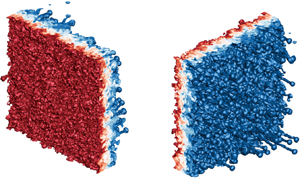
The mixing layer at late stages visualised from both the bubble and spike sides for cases 1 and 3 are shown in figure 3. Due to the presence of secondary instabilities, such as the KH instability, the bubbles with an initially rounded shape develop into numerous small irregular creases, and meanwhile the necks of the spikes undergo elongation and twisting. It is interesting that several faster-growing individual spikes behave like vortex rings, carrying a small amount of heavy fluid out of the mixing layer, which is consistent with the observation of Youngs (Reference Youngs2004). It is found that cases 1 and 2 present more such fast-growing spikes than case 3. The leading fronts of bubbles and spikes, $F_{b(s)}$, which are defined as the streamwise positions that represent 1 % volume fraction of air and SF$_6$ on the iso-surfaces, respectively, can be extracted (Thornber et al. Reference Thornber2017). Figure 4 shows the contours of bubble and spike fronts at early and late stages for cases 1 and 3. As we can see, the bubbles have undergone multiple generations of bubble merging, whereas the spikes develop into distinct vortex rings. The experimental results of Balakumar et al. (Reference Balakumar, Orlicz, Ristorcelli, Balasubramanian, Prestridge and Tomkins2012) and Balasubramanian, Orlicz & Prestridge (Reference Balasubramanian, Orlicz and Prestridge2013) showed that the mixing layer maintains the memory of initial large-scale perturbation even at the latest time of their experiments. To quantify this imprint, the correlation coefficients of bubble and spike fronts with respect to the initial distributions are calculated, which are defined as

(3.3)\begin{equation} I_{b(s)}=\dfrac{\langle F_{b(s),\tau}F_{b(s),0}\rangle -\langle F_{b(s),\tau}\rangle \langle F_{b(s),0}\rangle }{[(\langle F_{b(s),\tau}^2\rangle -\langle F_{b(s),\tau}\rangle ^2)(\langle F_{b(s),0}^2\rangle -\langle F_{b(s),0}\rangle ^2)]^{1/2}}. \end{equation}

Note higher values of $I_{b(s)}$ indicate more retention of the initial perturbation information. As shown in figure 5(a), the memory of the initial perturbations is forgotten faster and more for cases 1 and 2 than case 3, which implies that the large-scale perturbations are more persistent in the RM turbulence. It is also found that spikes retain a slightly stronger imprint about initial condition than bubbles.

Figure 3. Iso-surface of mass fraction for (a) case 1 at $\tau \approx 43.94$ and (b) case 3 at $\tau \approx 44.20$. Blue ($Y_{\text {SF}_6}=0.01$) and red ($Y_{\text {SF}_6}=0.99$) correspond to spikes and bubbles, respectively.

Figure 4. Contours of bubble and spike fronts.

Figure 5. Temporal evolutions of (a) the initial perturbation imprint measured by $I_{b(s)}$ and (b) the mean bubble wavelength $\langle \lambda _b\rangle$ calculated by (3.5).

The mean bubble wavelength can be calculated from figure 4 using the method of Dimonte et al. (Reference Dimonte2004). The first step is to obtain the autocorrelation function of the bubble front,

(3.4)\begin{equation} \eta_b(\kern0.7pt y,z)=\dfrac{\sum_{y^{\prime},z^{\prime}}(F_b(\kern0.7pt y^{\prime},z^{\prime})-\langle F_b\rangle )(F_b(\kern0.7pt y^{\prime}+y,z^{\prime}+z)-\langle F_b\rangle )}{\sum_{y^{\prime},z^{\prime}}(F_b(\kern0.7pt y^{\prime},z^{\prime})-\langle F_b\rangle )^2}. \end{equation}

Next, the mean diameter of the bubbles is estimated by identifying the radial position at which the azimuthally averaged value of $\eta _b$, $\langle \eta _b\rangle (r) = \langle \eta _b(\kern0.7pt y,z)\rangle |_{r=\sqrt {x^2+y^2}}$, is less than 0.3, i.e. $\langle D_b\rangle = r[\langle \eta _b\rangle (r)<0.3]$. The threshold of 0.3 is determined by testing the images containing objects with known diameters (Ramaprabhu, Dimonte & Andrews Reference Ramaprabhu, Dimonte and Andrews2005). Finally, the mean bubble wavelength is calculated with the relationship suggested by Daly (Reference Daly1967),

(3.5)\begin{equation} \langle \lambda_b\rangle \approx \langle D_b\rangle (\rho_h^+ +\rho_l^+)/\rho_h^+, \end{equation}

where $\rho _h^+$ and $\rho _l^+$ are the post-shock densities of the heavy and light gases, respectively. Combining the bubble front snapshot in figure 4 with the bubble wavelength evolution in figure 5(b), a possible physical scenario for the evolution of bubbles is presented as follows. After the impact of the incident shock, the bubble size experiences a rapid increment in all three cases. Later, as the bubbles are laterally squeezed, the bubbles in case 1 shrinks briefly, i.e. reduces in size. The squeezing process can also cause the inversion of the leading and trailing positions of the bubble front. This explains the negative correlation coefficient for case 1, as given in figure 5(a). For case 3, the existence of large-scale perturbations provides more space for small bubbles to expand, and thus the mean bubble size remains invariant for a certain period of time. The bubble size in case 2 falls between these two cases. At late stages, the bubble merging becomes pronounced, leading to the sustained growth of bubble size for all three cases.

The approach described in (3.4) and (3.5) extracts the dominant bubble wavelengths. As a supplement, we introduce Voronoi diagrams of bubble tips (Oron et al. Reference Oron, Arazi, Kartoon, Rikanati, Alon and Shvarts2001) to describe the bubble sizes more finely. Voronoi diagrams are a specific spatial tessellation that divides space into unique cells associated with each particular point (Ferenc & Néda Reference Ferenc and Néda2007; Monchaux, Bourgoin & Cartellier Reference Monchaux, Bourgoin and Cartellier2010). Each Voronoi cell contains the space that is closer to the corresponding particular point than to any other point. The Voronoi analysis has a wide range of applications in the field of fluid mechanics, such as describing the clustering of inertial particle (Monchaux et al. Reference Monchaux, Bourgoin and Cartellier2010; Brandt & Coletti Reference Brandt and Coletti2022) and the distribution of vortices (Osawa et al. Reference Osawa, Minamoto, Shimura and Tanahashi2021; Ding et al. Reference Ding, Ding, Chong, Wu, Xia and Zhong2023). In the RM and RT instabilities, this approach can be used to visualise the distribution of the bubbles (Kartoon et al. Reference Kartoon, Oron, Arazi and Shvarts2003).

Figure 6(ad) displays the 2-D Voronoi diagrams of bubbles for cases 1 and 3. To ensure closure of all sub-areas at the domain boundaries, ghost bubble tips based on periodicity are introduced (Jayaram et al. Reference Jayaram, Jie, Zhao and Andersson2020). It is seen that large bubbles in figure 4 are partitioned into several smaller bubbles in figure 6(ad) due to their non-smoothness. Therefore, this approach primarily measures the features of small bubbles. The probability density function (p.d.f.) of the bubble size can be obtained from the Voronoi diagrams, as shown in figure 6(e). The area of each Voronoi cell, $S$, is normalised by the mean value, $\langle S\rangle = S_d/N_p$, where $S_d$ and $N_p$ are the total area of the domain and the number of bubble tips, respectively. In $d$-dimensional space ($d=1,2,3$), the p.d.f. of the normalised Voronoi cell sizes for entities spatially distributed as a random Poisson process is well described by the $\varGamma$ distribution (Ferenc & Néda Reference Ferenc and Néda2007),

(3.6)\begin{equation} p_{\varGamma}(\kern0.7pt y) = \dfrac{[(3d+1)/2]^{(3d+1)/2}}{\varGamma[(3d+1)/2]}y^{(3d-1)/2}\exp (-[(3d+1)/2]y), \end{equation}

where $\varGamma (\kern0.7pt y)$ is the Gamma function. It is found that the distribution of bubble sizes approximately follows a random Poisson process for all three cases. This finding is useful for the bubble merger model (Alon, Shvarts & Mukamel Reference Alon, Shvarts and Mukamel1993; Alon et al. Reference Alon, Hecht, Mukamel and Shvarts1994, Reference Alon, Hecht, Ofer and Shvarts1995). As illustrated in figure 6f), the standard deviation of the normalised Voronoi areas of the bubble tips, $\sigma _{S/\langle S\rangle }$, is slightly higher than the value of the $\varGamma$ distribution, $\sigma _{\varGamma } = \sqrt {2/(3d+1)}$, particularly for case 3, which indicates the ‘clustering’ of bubbles (Monchaux et al. Reference Monchaux, Bourgoin and Cartellier2010; Tagawa et al. Reference Tagawa, Mercado, Prakash, Calzavarini, Sun and Lohse2012). The increasing trend also reflects the increasing bubble merging. Figure 6(g) shows the results of the second measurement of bubble wavelength,

(3.7)\begin{equation} \langle \lambda_b\rangle \approx \sqrt{\dfrac{\langle S\rangle }{\rm \pi}}, \end{equation}

which is more representative of small bubbles as mentioned earlier. The results indicate that there are many smaller bubbles produced at early times, which is particularly evident in case 1 and relatively weak in case 3. This may be the reason for the early decrease in the bubble wavelength for case 1, as shown in the first measurement in figure 5(b). Upon observing the proximity of the starting point of the increase in figure 6f,g), it is found that bubble merging derives the growth of bubble size. It is important to note that, although two distinct approaches are employed to measure bubble sizes, aiming to enhance the robustness of our conclusions regarding bubble size evolution, factors such as diffusion, bubble tilting and coverage collectively diminish the effectiveness of these measurements, particularly in the early stages of establishing self-similar order.

Figure 6. (ad) Voronoi cells (blue lines) of bubble tips (red dots). Data are from (a,b) case 1 and (c,d) case 3 at (a,c) $\tau \approx 4$ and (b,d) $\tau \approx 44$. Localised diagrams are used for clarity. (e) The p.d.f. of normalised Voronoi areas $S/\langle S\rangle$. Open symbols: $\tau \approx 4$. Solid symbols: $\tau \approx 44$. ( f) Temporal evolution of scaled standard deviation $\sigma _{S/\langle S\rangle }/\sigma _{\varGamma }$. (g) Temporal evolution of the mean bubble wavelength $\langle \lambda _b\rangle$ calculated by (3.7).

For the entire mixing layer, the mixing width can be calculated by integrating the averaged volume fractions (e.g. Thornber et al. Reference Thornber, Drikakis, Youngs and Williams2010),

(3.8)\begin{equation} W = \int 4\langle\, f_1 \rangle_{yz} \langle\, f_2 \rangle_{yz}\,{\rm d}\kern0.7pt x. \end{equation}

Note the evolutions of the mixing width for cases 1 and 3 have been reported in our previous work (Zhou et al. Reference Zhou, Ding, Cheng and Luo2023a). Here, it is found that the mixing width in case 2 is nearly identical to that of case 1. In addition, the growth rate of the mixing width, $\theta$, has a fitted value of 0.220 in case 2 that is nearly identical to 0.211 in case 1, whereas the fitted value of $\theta$ in case 3 is notably higher ($\theta = 0.333$) (Zhou et al. Reference Zhou, Ding, Cheng and Luo2023a). The value of $\theta$ in the broadband case is lower than the model prediction value $0.4$ (Youngs Reference Youngs2004; Soulard et al. Reference Soulard, Guillois, Griffond, Sabelnikov and Simoëns2018). One possible reason is that the total standard deviation of the perturbation is fixed at $\sigma _0 = 0.5\lambda _{min}$ for reaching the turbulent state faster, which violates the early linearity-ensuring (Thornber et al. Reference Thornber, Drikakis, Youngs and Williams2010; Groom & Thornber Reference Groom and Thornber2020). Therefore, simulations in the present work deviate to some extent from the linear assumption adopted by the model. This may be a reason for the discrepancy between the present simulation and the model prediction. In addition, limited bandwidth for the present simulations may also have a certain influence on the value of $\theta$ (Groom & Thornber Reference Groom and Thornber2020). It indicates that the mixing width evolution tends to remain the same if the initial perturbation bandwidth is narrowed towards a high wavenumber, revealing an insensitivity of the RM mixing layer to initial perturbations. This finding is consistent with the theoretical proposal of Elbaz & Shvarts (Reference Elbaz and Shvarts2018) and Soulard et al. (Reference Soulard, Guillois, Griffond, Sabelnikov and Simoëns2018). They found that the evolution of the mixing width is influenced by both the characteristics of large-scale structures and the nonlinear interactions of small-scale structures, and the sole presence of small-scale structures could lead to similar evolution results for cases with narrowband, short-wavelength perturbations. A detailed explanation of the similarity between case 1 and case 2 is given hereinafter from various perspectives.

3.2. Turbulent kinetic energy

For the RM turbulence, the shock–interface interaction is the primary source of kinetic energy. The kinetic energy deposited at the early stage is subsequently transferred to various scales and ultimately dissipated into internal energy by viscosity in an irreversible manner. It has been found that the RM turbulence at the self-similar stage is analogous to the decaying turbulence (Thornber & Zhou Reference Thornber and Zhou2012; Tritschler et al. Reference Tritschler, Zubel, Hickel and Adams2014b), and the growth rate exponent $\theta$ of the mixing width is closely related to the decay rate exponent $n$ of TKE,

(3.9)\begin{equation} n = 2 - 2\theta. \end{equation}

This relationship can be obtained through dimensional analysis (Thornber et al. Reference Thornber, Drikakis, Youngs and Williams2010), $\sqrt {\text {TKE}}\propto \text {d}W/\text {d}t\propto t^{\theta -1}$. The decay rate of the integral TKE (ITKE) can be estimated by utilising the mean TKE in conjunction with the mixing width $W$, i.e. $\text {ITKE}\propto W*\text {TKE}\propto t^{-(n-\theta )}$, where

(3.10a,b)\begin{equation} \text{ITKE} = \int \text{TKE}(x)L_0^2\,\text{d}\kern0.7pt x,\quad \text{TKE}(x)=\left\langle \dfrac{1}{2}\rho u_i^{\prime\prime}u_i^{\prime\prime}\right\rangle_{yz}. \end{equation}

Both ITKE and TKE (shown here with its maximum value) experience an exponential decay that is compatible with (3.9) at late stages, as seen in figure 7. It is also found that, the curves here for case 1 and case 2 almost collapse with each other.

Figure 7. Temporal evolutions of TKE for (a) case 1, (b) case 2 and (c) case 3. The dash-dotted and dashed lines represent $\propto \tau ^{-(2-2\theta )}$ and $\propto \tau ^{-(2-3\theta )}$, respectively, where $\theta$ is assigned the fitted value.

Figure 8 displays the spatial distribution of the mean TKE along the $x$ axis for the three cases, where the horizontal coordinate is normalised with the mixing width $W$ and the mixing layer centre $x_c$ (Walchli & Thornber Reference Walchli and Thornber2017) that is determined by

(3.11)\begin{equation} \int_{-\infty}^{x_c}\langle\, f_2 \rangle = \int_{x_c}^{\infty}\langle\, f_1 \rangle\,{\rm d}\kern0.7pt x. \end{equation}

It is shown that the peak of the mean TKE does not occur at the centre of the mixing layer, but is biased towards the spike side (i.e. $(x-x_c)/W<0$), similar to the asymmetric results of Groom & Thornber (Reference Groom and Thornber2023). It indicates that turbulent fluctuations are more active in the spike region. As time proceeds, the distribution curves for the three cases deviate. The curves for case 1 and case 2 exhibit greater irregularity with longer and more complex tails on the spike side, whereas the curve for case 3 is closer to the Gaussian curve with a smoother tail. This is consistent with the observation in figure 3 that for cases 1 and 2 there are numerous small vortex rings ejected from the head of fast-growing spikes, and their scaling behaviour differs from the rest region of the mixing layer (Thornber et al. Reference Thornber, Griffond, Bigdelou, Boureima, Ramaprabhu, Schilling and Williams2019). The distribution curves of TKE for the three cases converge when $\tau > 30$, which indicates the reach of a self-similar state.

Figure 8. The profiles of plane-averaged TKE along the $x$-direction for (a) case 1, (b) case 2 and (c) case 3 at various moments.

3.3. Mixing measures

To quantify the mixing degree within the mixing zone, two mixing metrics are introduced: the molecular mixing fraction $\varTheta$ (Youngs Reference Youngs1991) and the mixing parameter $\varXi$ (Cook & Zhou Reference Cook and Zhou2002; Thornber et al. Reference Thornber, Drikakis, Youngs and Williams2010), which are respectively given by

(3.12)$$\begin{gather} \varTheta = \dfrac{\displaystyle\int \langle\, f_1 f_2 \rangle\,{\rm d}\kern0.7pt x}{\displaystyle\int \langle\, f_1 \rangle \langle\, f_2 \rangle\,{\rm d}\kern0.7pt x}, \end{gather}$$
(3.13)$$\begin{gather}\varXi = \dfrac{\displaystyle\int \langle {\rm min}(f_1,f_2) \rangle\,{\rm d}\kern0.7pt x}{\displaystyle\int {\rm min}(\langle\, f_1 \rangle,\langle\, f_2 \rangle)\,{\rm d}\kern0.7pt x}. \end{gather}$$

As shown in figure 9, for each case, $\varTheta$ and $\varXi$ have similar evolution trends and asymptotic values. The curves for cases 1 and 2 almost overlap, whereas the curve for case 3 has a lower asymptotic value and enters the plateau stage earlier ($\tau \approx 20$ for case 3, $\tau \approx 30$ for cases 1 and 2). The emergence of the plateau stage also indicates the self-similar evolution of the mixing layer. According to the theory of Soulard et al. (Reference Soulard, Guillois, Griffond, Sabelnikov and Simoëns2018), there is a relationship between the molecular mixing fraction $\varTheta$ and the growth rate exponent $\theta$ of the mixing width:

(3.14)\begin{equation} \varTheta_1 = \dfrac{2-3\theta}{2+(n_p-3)\theta}\quad \left(\theta\leq \dfrac{2}{3}\right), \end{equation}

where the coefficient $n_p$ is related to the proportional contribution of large and small scales to the energy and concentration spectra. Equation (3.14) illustrates that $\varTheta$ decreases as $\theta$ increases, namely, the degree of mixing is inversely related to the growth rate of the mixing layer. This finding aligns with the results depicted in figure 9, wherein case 3 with broadband perturbations exhibits a higher mixing width growth rate but a lower mixing degree.

Figure 9. Temporal evolutions of (a) the molecular mixing fraction, $\varTheta$, and (b) the mixing parameter, $\varXi$.

By applying mathematical analysis of partial differential equations, Doss (Reference Doss2022) examined the mass transport within a decaying turbulence field, which is a specific critical class balanced between wave-like convection and heat-like diffusion. The author then extended this theory to the RM turbulence, obtaining a relationship between the molecular mixing fraction and the diffusion parameter $\mu =n(2C_{\theta }-1)/(2-n)$:

(3.15)\begin{equation} \varTheta_2 =1-\dfrac{\mu_c}{\mu}=\dfrac{2C_{\theta}-1-(2C_{\theta}-1+\mu_c)\theta} {(2C_{\theta}-1)(1-\theta)}, \end{equation}

where $C_{\theta }$ is the Monin constant (Pope Reference Pope1994) and $\mu _c=1$. Although models (3.14) and (3.15) are developed with two different methods and assumptions, they can match if the free parameters of one model are adjusted to the conventions of the other (Doss Reference Doss2022). The connection between $\varTheta$ and $\theta$ for the three cases at the plateau stage is given in figure 10, where the prediction curves of models (3.14) and (3.15) are also provided. It is worth noting that these curves collapse perfectly when the value of $n_p$ in the former model is set to 1.0 and the value of $C_{\theta }$ in the latter model is adjusted to 3/2. At the plateau stage, all numerical results fall within the range between the two models and also show consistent variation trend with the model predictions. This suggests again that the mixing layer grows more slowly, but more efficiently, for cases with narrowband, short-wavelength perturbations. The present finding demonstrates the validity of the theoretical models.

Figure 10. Variations of the molecular mixing fraction, $\varTheta$, vs the mixing width growth rate, $\theta$. The solid and dash-dotted lines represent the relationship curves obtained by taking $n_{p}$ in (3.14) as that in (3.9) and $1.1$, respectively; the dashed line represents the curve obtained by using $C_{\theta }=3/2$ in (3.15). The symbols denote the values of $\varTheta$ at the plateau stage.

In addition, the mixing level can be assessed by calculating the p.d.f. of $Y_{\text {SF}_6}$ within the mixing zone. For a dataset of physical quantity $\varphi$, dividing its values equally into $N_b$ bins within the range $[\varphi _{min},\varphi _{max}]$, the discrete p.d.f. of $\varphi$ in the $k$th bin is

(3.16)\begin{equation} \text{p.d.f.} = \dfrac{N_k}{(\Delta\varphi)N}, \end{equation}

where $N$ and $N_k$ are the total number of data points within the dataset and the $k$th bin, respectively. Here $\Delta \varphi = {(\varphi _{max} - \varphi _{min})}/{N_b}$ represents the bin spacing, and $\sum _{k=1}^{N_b}\text {p.d.f.}\Delta \varphi =1$. In this work, $N_b=64$ is adopted, and the dataset is taken as the data in the inner mixing zone (IMZ), where the IMZ is defined as the set of cross-flow planes satisfying the following condition (Tritschler et al. Reference Tritschler, Olson, Lele, Hickel, Hu and Adams2014a):

(3.17)\begin{equation} 4\langle Y\rangle_{yz}(1-\langle Y\rangle_{yz})\geq 0.9. \end{equation}

Figure 11 displays the p.d.f.s of the mass fraction of SF$_6$ in the range $0.1\leq Y_{\text {SF}_6}\leq 0.9$ at the post-shock moment ($\tau \approx 0.3$), the early stage ($\tau \approx 4$), the transition stage ($\tau \approx 15$) and the plateau stage ($\tau > 30$) for all three cases. It should be noted that in the p.d.f. curve of $Y_{{SF}_6}$, the mixing degree is higher for a single peak than for double peaks. In addition, for the single peak situation, the mixing is higher when the peak is narrower (i.e. smaller variance) and the tail is thinner (i.e. lower kurtosis). At $\tau \approx 0.3$, the p.d.f.s of $Y_{{SF}_6}$ show a distinct bimodal distribution with two peaks at the boundaries, which indicates that the fluids in the IMZ are in a nearly separated state. At $\tau \approx 4$, the curves for all three cases converge to a state with a single peak, whose position leans toward the heavy fluid side. The presence of tail buckling in the curves suggests the existence of a substantial amount of pure, unmixed fluids at this moment. At the transition stage ($\tau \approx 15$), the two gases in the IMZ have already reached a high degree of mixing, and the p.d.f. curves show a nearly Gaussian distribution around $Y_{{SF}_6}=0.5$. At the plateau stage ($\tau > 30$), the p.d.f. within the IMZ maintains the Gaussian distribution. Afterwards, the peak value decreases and the tail widens, indicating the transfer of partially mixed fluids from the border of mixing zone into the IMZ for further mixing. In addition, the p.d.f.s of SF$_6$ within the IMZ tend to converge to a single curve for each case, which implies a dynamic equilibrium between the expanding mixing zone and the mixing occurring within the mixing layer. It is found that case 3 exhibits a lower level of mixing within the IMZ than cases 1 and 2, which aligns with the aforementioned finding.

Figure 11. The p.d.f.s of $\text {SF}_6$ mass fraction, $Y_{{SF}_6}$, within the IMZ for (a) case 1, (b) case 2 and (c) case 3.

3.4. Anisotropy and inhomogeneity

The RM turbulence is highly anisotropic and inhomogeneous due to the inherent directionality of both the moving shock wave and the initial perturbations. The evolutions of anisotropy, characterised by the ratio of velocity fluctuations in different directions (Tritschler et al. Reference Tritschler, Olson, Lele, Hickel, Hu and Adams2014a), and inhomogeneity, measured by density self-correlation (DSC) (Besnard et al. Reference Besnard, Harlow, Rauenzahn and Zemach1992), within the mixing zone ($0.01\le \langle Y\rangle _{yz}\le 0.99$) for all three cases are plotted in figure 12. The two quantities are defined, respectively, as

(3.18)$$\begin{gather} a = \dfrac{\lvert u^{\prime\prime} \rvert}{\lvert u^{\prime\prime} \rvert + \lvert v^{\prime\prime} \rvert + \lvert w^{\prime\prime} \rvert}-\frac{1}{3}, \end{gather}$$
(3.19)$$\begin{gather}b ={-}\left\langle \left(\frac{1}{\rho}\right)^{\prime} \rho^{\prime} \right\rangle = \left\langle \frac{1}{\rho} \right\rangle \langle \rho \rangle -1. \end{gather}$$

The value of $a$ ranges from $-1/3$ to $2/3$. The lower and upper limits correspond to the absence of TKE in the streamwise and spanwise directions, respectively. The value of $a=0$ corresponds to an isotropic state. DSC is a non-negative parameter. Its zero value corresponds to homogeneous mixing, and higher DSC values indicate increased spatial inhomogeneity and a lower degree of mixing. At the late stage, the RM turbulence decreases in anisotropy with time. Despite this, the RM turbulence seems hard to reach complete isotropy as suggested by the curve variation tendency (Tritschler et al. Reference Tritschler, Olson, Lele, Hickel, Hu and Adams2014a; Thornber et al. Reference Thornber2017; Sewell et al. Reference Sewell, Ferguson, Krivets and Jacobs2021). The indicators of anisotropy and inhomogeneity reach stable values at the self-similarity stage, but are different among the three cases. Specifically, the degree of anisotropy and inhomogeneity is higher for case 3 than for cases 1 and 2, and the evolution curves for cases 1 and 2 almost overlap. The asymptotic values for both cases 1 and 2 are $\langle a\rangle _{MZ}\approx 0.087$ and $\langle b\rangle _{MZ}\approx 0.077$, whereas the asymptotic values for case 3 are $\langle a\rangle _{MZ}\approx 0.119$ and $\langle b\rangle _{MZ}\approx 0.155$. Since $a$ and $b$ are large-scale metrics, this result is consistent with the fact that case 3 has initial large-scale perturbations.

Figure 12. Temporal evolutions of (a) the mean anisotropy, $\langle a\rangle _{MZ}$, and (b) DSC, $\langle b\rangle _{MZ}$, within the mixing zone.

4. Inter-scale energy transfer

One of the main objectives of the present study is to examine the inter-scale energy transfer in RM turbulence. In particular, the difference in the inter-scale energy transfer among cases 1, 2 and 3, where the energy is initially deposited at different scales, are analysed. For this purpose, a coarse-graining approach is adopted to expose the inter-scale energy fluxes at selected specific scales.

4.1. Coarse-grained method

The coarse-graining approach, which has the same form as the modelling of large-eddy simulation of turbulence, was intended primarily to probe the sub-scale physical processes (Germano Reference Germano1992; Aluie Reference Aluie2013). When a field $\boldsymbol {f}(\boldsymbol {x})$ is subjected to low-pass filtering, it retains only the scales with sizes $\geq \ell$. This process can be regarded as an $n-D$ convolution

(4.1)\begin{equation} \bar{\boldsymbol{f}}(\boldsymbol{x})= G_{\ell}\star \boldsymbol{f} = \int \text{d}^n\boldsymbol{r} G_{\ell}(\boldsymbol{x}-\boldsymbol{r}) \boldsymbol{f}(\boldsymbol{r}), \end{equation}

where $G(\boldsymbol {r})$ is the normalised convolution/filtering kernel, i.e. for dimensionless $\boldsymbol {s}$, $\int \text {d}^n\boldsymbol {s} G(\boldsymbol {s})=1$. To achieve filtering, the real function $G(\boldsymbol {r})$ should exhibit a rapid decay as $\boldsymbol {r}$ becomes larger. Here $G_{\ell }(\boldsymbol {r}) \equiv \ell ^{-n}G(\boldsymbol {r}/\ell )$ is the $n$-dimensional; dilation kernel for $G(\boldsymbol {r})$ and its main support is within the region of diameter $\ell$. Thus, (4.1) can be regarded as a local spatial average. After the coarse graining, the field $\boldsymbol {f}(\boldsymbol {x})$ is decomposed into a large-scale ($\gtrsim \ell$) component $\bar {\boldsymbol {f}}_{\ell }$ and a small-scale ($\lesssim \ell$) component $\boldsymbol {f}^{\prime }_{\ell }=\boldsymbol {f}-\bar {\boldsymbol {f}}_{\ell }$. In this work, we adopt the Gaussian filter kernel, which is commonly used in physical space filtering:

(4.2)\begin{equation} G_{\ell}(\boldsymbol{x}-\boldsymbol{r}) = \left(\dfrac{\gamma}{{\rm \pi} \ell^2}\right)^{n/2}\exp \left(-\dfrac{\gamma \lvert \boldsymbol{x-r} \rvert^2}{\ell^2}\right), \end{equation}

where $\gamma$ is a constant that usually takes the value $\gamma =6$, and the standard deviation is $\sigma ={\ell }/{\sqrt {2\gamma }}$. The Gaussian filter kernel remains positive in the physical space, thereby avoiding the occurrence of unphysical negative densities during the filtering process (Wang et al. Reference Wang, Wan, Chen and Chen2018). The proper scale decomposition for variable-density flows is not as straightforward as it is for incompressible flows. A more suitable approach in such cases is the utilisation of Favre filtering (Garnier, Adams & Sagaut Reference Garnier, Adams and Sagaut2009)

(4.3)\begin{equation} \tilde{f}=\overline{\rho f}/\bar{\rho}. \end{equation}

As shown by Aluie (Reference Aluie2013) and Zhao & Aluie (Reference Zhao and Aluie2018), the Favre filtering satisfies the inviscid criterion for arbitrarily large density variations.

Subsequently, the budget for kinetic energy at large scales ($\gtrsim \ell$) can be derived by filtering the momentum equation in the N–S equations

(4.4)$$\begin{gather} \partial_{t}\left(\bar{\rho}\dfrac{\lvert \tilde{\boldsymbol{u}}_{\ell} \rvert^2}{2}\right) + \boldsymbol{\nabla}\boldsymbol{\cdot} \boldsymbol{J}_{\ell} ={-}\varPi_{\ell} - \varPhi_{\ell} - D_{\ell} + \epsilon^{inj}_{\ell}, \end{gather}$$
(4.5)$$\begin{gather}(J_{\ell})_j = \bar{\rho}\frac{\lvert \tilde{\boldsymbol{u}} \rvert^2}{2}\tilde{u}_j + \bar{p}\tilde{u}_j + \tilde{u}_i\bar{\rho}\tilde{\tau}(u_i,u_j) - \tilde{u}_i\bar{\sigma}_{ij}, \end{gather}$$
(4.6)$$\begin{gather}\varPi_{\ell}={-}\bar{\rho}\partial_j\tilde{u}_i\tilde{\tau}(u_i,u_j), \end{gather}$$
(4.7)$$\begin{gather}\varPhi_{\ell} ={-} \bar{p}_{\ell}\boldsymbol{\nabla}\boldsymbol{\cdot}\tilde{\boldsymbol{u}}_{\ell}, \end{gather}$$
(4.8)$$\begin{gather}D_{\ell}=\partial_j\tilde{u}_i\bar{\sigma}_{ij}, \end{gather}$$
(4.9)$$\begin{gather}\epsilon^{\rm inj}_{\ell}=\tilde{u}_i\bar{\rho}\tilde{F}_i, \end{gather}$$

where $\boldsymbol {J}_{\ell }$, $\varPhi _{\ell }$, $D_{\ell }$ and $\epsilon ^{\rm inj}_{\ell }$ are the spatial transports for the kinetic energy, the large-scale pressure dilatation, the viscous dissipation and the kinetic energy injection, respectively. Here $\tilde {\tau }(f,g) \equiv \widetilde {(fg)}_{\ell }-\tilde {f}_{\ell }\tilde {g}_{\ell }$ is the second-order generalised central moment for the fields $f(\boldsymbol {x})$ and $g(\boldsymbol {x})$ (Germano Reference Germano1992). We use $\varPi _{\ell }$ to denote the inter-scale energy flux (also known as SFS energy flux) in the budget (4.4), which is produced by the large-scale strain $\partial _j\tilde {u}_i$ against the small-scale turbulent stress $\bar {\rho }\tilde {\tau }(u_i,u_j)$ (Aluie Reference Aluie2011) and thus referred to as the deformation work. This form of large-scale kinetic energy budget is commonly used in turbulence studies, especially for incompressible flows. Recent studies (Aluie Reference Aluie2011, Reference Aluie2013) found that there is another pathway of energy transfer between scales for compressible flows, which is concealed in the form of (4.4). In fact, the derivation of (4.4) takes $\tilde {u}_i\partial _i\bar {p}$ in the following form

(4.10)\begin{equation} \tilde{u}_i\partial_i\bar{p} = \partial_i(\tilde{u}_i\bar{p})-\bar{p}\partial_i\tilde{u}_i. \end{equation}

Rewritten in another equivalent form, namely

(4.11)\begin{equation} \tilde{u}_i\partial_i\bar{p} = \dfrac{1}{\bar{\rho}}\partial_i\bar{p}\bar{\tau}(\rho,u_i) +\partial_i(\bar{p}\bar{u}_i)-\bar{p}\partial_i\bar{u}_i, \end{equation}

(4.4) can be transformed to

(4.12)\begin{equation} \partial_{t}\left(\bar{\rho}\dfrac{\lvert \tilde{\boldsymbol{u}}_{\ell} \rvert^2}{2}\right) + \boldsymbol{\nabla}\boldsymbol{\cdot} \boldsymbol{J}_{\ell} ={-}\varPi_{\ell} -\varLambda_{\ell} - \varPhi_{\ell} - D_{\ell} + \epsilon^{inj}_{\ell}. \end{equation}

The spatial transfer and pressure-dilatation terms in the above equation become

(4.13)\begin{equation} (J_{\ell})_j = \bar{\rho}\dfrac{\lvert \tilde{\boldsymbol{u}} \rvert^2}{2}\tilde{u}_j + \bar{p}\bar{u}_j + \tilde{u}_i\bar{\rho}\tilde{\tau}(u_i,u_j) - \tilde{u}_i\bar{\sigma}_{ij}, \end{equation}

and

(4.14)\begin{equation} \varPhi_{\ell} ={-} \bar{p}_{\ell}\boldsymbol{\nabla}\boldsymbol{\cdot}\bar{\boldsymbol{u}}_{\ell}, \end{equation}

respectively. The rest of the terms with the same notation as in (4.4) remain unchanged. Another inter-scale energy flux, newly derived in (4.12), is called baropycnal work, which has the form

(4.15)\begin{equation} \varLambda_{\ell} = \dfrac{1}{\bar{\rho}}\partial_j\bar{p}\bar{\tau}(\rho,u_j). \end{equation}

This term arises from the action of large-scale pressure gradient $\partial _j\bar {p}/\bar {\rho }$ on the small-scale turbulent mass flux $\bar {\tau }(\rho,u_j)$, which is present only in flows with density variation. In (4.12), the positive $\varPi _{\ell }$ and $\varLambda _{\ell }$ denote the forward transfer of TKE from large scales ($\gtrsim \ell$) to small scale ($\lesssim \ell$), whereas the negative versions denote the inverse transfer of TKE from small scale ($\lesssim \ell$) to large scale ($\gtrsim \ell$).

4.2. Inter-scale energy fluxes

This subsection focuses on the evolutions of the two inter-scale energy fluxes in budget (4.12) with filter scales of $k_{\ell }=16$, $k_{\ell }=32$ and $k_{\ell }=48$. As illustrated in figure 2, the scale $k_{\ell }=32$ is initially involved for all three cases, and $k_{\ell }=16$ and $k_{\ell }=48$ represent the upper and lower limits of the initial perturbation spectrum in case 2. Temporal evolutions of the two inter-scale energy fluxes averaged in the mixing zone at the filter scales $k_{\ell }=16$, $k_{\ell }=32$, and $k_{\ell }=48$ are plotted in figure 13. It should be noted that the data are plotted in log–log scale. When $\langle \varPi _{\ell }\rangle _{MZ}$ and $\langle \varLambda _{\ell }\rangle _{MZ}$ are non-positive, they hold no meaning and thus are plotted by their absolute values in the figure. In figure 13(a), the deformation work at all three scales exhibits an inverse transfer at the early stage, then shifts to the forward transfer. It indicates that vorticity initially deposited at the interface forms large vortical structures at the early stage and, subsequently, small vortical structures are generated as a result of the deformation process. As shown in figure 13(b), the mean baropycnal work curves for all three cases almost overlap at the early stage and show a forward transfer behaviour. Subsequently, they shift to a brief period of inverse transfer and return eventually to the forward transfer. At the late stage, notable difference among the three cases is observed, which is similar to the evolution of the mixing features (see figures 9 and 12). Both energy fluxes exhibit exponential decay at the self-similar stage for each case. The decay exponent of deformation work shows a larger difference than that of baropycnal work at each scale, whereas its decay exponent on the largest filter scale is comparable to that of the ITKE.

Figure 13. Temporal evolutions of (a) deformation work, $\varPi _{\ell }$, and (b) baropycnal work, $\varLambda _{\ell }$, at three filter scales within the mixing zone. Absolute values are plotted using lines for positive data and symbols for no-positive data. The red, yellow and blue represent the results for case 1, case 2 and case 3, respectively. All results in the figure have been normalised by $\bar {\rho }^{+}(\Delta U)^3/\bar {\lambda }$.

Due to anisotropy of RM turbulence, it is necessary to conduct a directional examination of the SFS energy fluxes. To this end, the SFS energy fluxes are expressed in the form of directional components, enabling the assessment of anisotropy at various scales within the mixing layer. The mean SFS energy flux fraction is defined as

(4.16) \begin{equation} \left.\begin{array}{c@{}} c_{\varPi_{\ell}^{\xi}} = \dfrac{\langle \varPi_{\ell}^{\xi}\rangle } {\lvert\langle \varPi_{\ell}^{x}\rangle \rvert+\lvert\langle \varPi_{\ell}^{y}\rangle \rvert +\lvert\langle \varPi_{\ell}^{z}\rangle \rvert},\\ c_{\varLambda_{\ell}^{\xi}} = \dfrac{\langle \varLambda_{\ell}^{\xi}\rangle }{\lvert\langle \varLambda_{\ell}^{x}\rangle \rvert+\lvert\langle \varLambda_{\ell}^{y}\rangle \rvert+\lvert\langle \varLambda_{\ell}^{z}\rangle \rvert}, \end{array}\right\} \end{equation}

where $\varPi _{\ell }^{\xi }=-\bar {\rho }\partial _j\tilde {u}_{\xi }\tilde {\tau }(u_{\xi },u_j)$ and $\varLambda ^{\xi }_{\ell }=({1}/{\bar {\rho }})\partial _{\xi }\bar {p}\bar {\tau }(\rho,u_{\xi })$ with $\xi$ being the $x$, $y$ or $z$ direction. Note the signs of the fluxes are incorporated into the definition, and we have $\sum \lvert c_{\varPi _{\ell }^{\xi }(\varLambda _{\ell }^{\xi })}\rvert =1$. Temporal evolutions of the mean SFS energy flux fraction for all three cases are plotted in figure 14. The $y$ and $z$ components are consistent with each other, which indicates the statistical isotropy in the cross-flow direction. The $x$ component is always greater than the other two components. This gives the evidence of anisotropy at all three scales and also emphasises the necessity of considering anisotropy when modelling the RM turbulence. As the filter scale decreases, the anisotropy measure in the SFS energy flux decreases, which is in accordance with the findings of Lombardini, Pullin & Meiron (Reference Lombardini, Pullin and Meiron2012), Mansoor et al. (Reference Mansoor, Dalton, Martinez, Desjardins, Charonko and Prestridge2020) and Mohaghar et al. (Reference Mohaghar, Carter, Musci, Reilly, McFarland and Ranjan2017) regarding the local isotropy of the energy spectrum. The comparison among the three cases shows that the anisotropy measure of the deformation work for case 3 is greater than that of cases 1 and 2 at all three scales, which is consistent with the results in figure 12. Considering the initial narrowband perturbations in cases 1 and 2 are naturally different from the initial broadband perturbation in case 3, the findings here suggest that the anisotropy caused by the scale evolution is greater than that caused by interactions with other (anisotropic) scales. This also implies that symmetry breaking is gradually weakened during the interactions between scales. Unlike the deformation work, the anisotropy measure of the baropycnal work shows no significant difference among the three cases. The inverse transfer of baropycnal work is predominantly observed in the $x$ direction, and case 3 shows a longer period of dominance in this inverse transfer compared with cases 1 and 2.

Figure 14. Temporal evolutions of the mean SFS energy fluxes (a,c,e) $c_{\varPi _{\ell }^{\xi }}$ and (b,df) $c_{\varLambda _{\ell }^{\xi }}$ within the mixing zone. Data are from (a,b) case 1, (c,d) case 2 and (ef) case 3. The blue, red and yellow lines represent $\xi =x$, $y$ and $z$, respectively.

4.3. Nonlinear model of baropycnal work

The distinct behaviours of the two SFS energy fluxes imply that they might be governed by different physical mechanisms. Previous studies suggested that the deformation work is linked to processes involving vortex stretching and strain self-amplification (Carbone & Bragg Reference Carbone and Bragg2020; Johnson Reference Johnson2020, Reference Johnson2021), whereas the mechanisms of the baropycnal work in variable-density turbulence remain unclear. Inspired by the theoretical work of Borue & Orszag (Reference Borue and Orszag1998) and Eyink (Reference Eyink2006), Lees & Aluie (Reference Lees and Aluie2019) derived a nonlinear model for baropycnal work,

(4.17)\begin{align} \varLambda_{\ell}(\boldsymbol{x}) \approx \varLambda_{m,\ell}(\boldsymbol{x}) & = \frac{1}{3}C_2\ell^2\frac{1}{\bar{\rho}}(\partial_j\bar{p}\partial_k\bar{\rho}\partial_k\bar{u}_j)\nonumber\\ & =\dfrac{1}{3}C_2\ell^2\dfrac{1}{\bar{\rho}}\left[\boldsymbol{\nabla}\bar{p}\boldsymbol{\cdot}\bar{\boldsymbol{\mathsf{S}}} \boldsymbol{\cdot}\boldsymbol{\nabla}\bar{\rho}+\dfrac{1}{2}\bar{\boldsymbol{\omega}}\boldsymbol{\cdot}(\boldsymbol{\nabla}\bar{\rho} \times\boldsymbol{\nabla}\bar{p})\right]\nonumber\\ & = \varLambda_{\text{SR},\ell} + \varLambda_{\text{BC},\ell}. \end{align}

Here, $\varLambda _\text {SR}$ and $\varLambda _{BC}$ represent the strain generation process and the baroclinic vorticity generation process, respectively, which are given as

(4.18)$$\begin{gather} \varLambda_{\text{SR},\ell}=\dfrac{1}{3}C_2\ell^2\dfrac{1}{\bar{\rho}}[\boldsymbol{\nabla}\bar{p}\boldsymbol{\cdot} \bar{\boldsymbol{\mathsf{S}}}\boldsymbol{\cdot}\boldsymbol{\nabla}\bar{\rho}]=\dfrac{1}{3}C_2\ell^2 \dfrac{1}{\bar{\rho}}\partial_j\bar{p}\partial_k\bar{\rho}\bar{S}_{kj}, \end{gather}$$
(4.19)$$\begin{gather}\varLambda_{\text{BC},\ell} = \dfrac{ 1}{3}C_2\ell^2\dfrac{1}{\bar{\rho}}\left[\dfrac{1}{2}\bar{\boldsymbol{\omega}}\boldsymbol{\cdot}(\boldsymbol{\nabla}\bar{\rho} \times\boldsymbol{\nabla}\bar{p})\right]=\dfrac{1}{3}C_2\ell^2\dfrac{1}{\bar{\rho}} \dfrac{1}{2}\partial_j\bar{p}\partial_k\bar{\rho}\epsilon_{kjs}\bar{\omega}_s. \end{gather}$$

In (4.17), $C_{\iota }$ is the $\iota$th-order moment of the filter kernel. For the Gaussian filter kernel adopted here, $C_{\iota }$ is given as

(4.20)\begin{equation} C_{\iota} = \int\text{d}^{3}\boldsymbol{r} G(\boldsymbol{r})\lvert \boldsymbol{r}^{\iota} \rvert = \dfrac{\iota+1}{\sqrt{\rm \pi}}\gamma^{-\frac{\iota}{2}}\varGamma\left(\dfrac{\iota+1}{2}\right), \end{equation}

where $\varGamma (x)$ is the Gamma function, and we have $C_{2}={3}/{2\gamma }$. The nonlinear model (4.17) indicates that the baropycnal work transfers energy between scales through two pathways: one associated with baroclinic generation of vorticity and the other linked to strain generation caused by the pressure and density gradients (both barotropic and baroclinic). This model has recently been successfully applied to a priori test in forced compressible turbulence (Lees & Aluie Reference Lees and Aluie2019). To the best of the authors’ knowledge, this is the first time the performance of this model has been examined in relation to RM turbulence.

Figure 15 shows snapshots of the SFS energy fluxes at the mixing layer centre at $\tau =44$ for case 1. The other two cases have similar results and thus are not shown here. It is evident that the active regions of SFS energy fluxes display a speckled pattern at smaller filter scales and a chunky pattern at larger filter scales. Both forward and inverse transfers of deformation work are noticeably distinguishable at the larger filter scale, whereas the forward transfer region dominates at the smaller filter scale. There are distinct regions with positive and negative baropycnal work on both large and small filter scales. This implies that the inverse transfer of deformation work primarily occurs at large scales, whereas the inverse transfer of baropycnal work is prevalent at both large and small scales. The snapshots of $\varLambda _{m,\ell }$ computed from the simulation data using the nonlinear model (4.17) are also given in figure 15. The predictions of this nonlinear model are very similar to the simulation results, especially at $k_{\ell }=32$ and $k_{\ell }=48$.

Figure 15. Snapshots of (a,d,g) the deformation work, $\varPi _{\ell }$, (b,e,h) baropycnal work, $\varLambda _{\ell }$, and (cf,i) the nonlinear model, $\varLambda _{m,\ell }$, for case 1 at $\tau =43.94$ at the central plane of the mixing layer. (a,b,c) $k_{\ell }=16$, (d,ef) $k_{\ell }=32$ and (g,h,i) $k_{\ell }=48$. The SFS energy fluxes in the figure have been normalised using their variances.

The relevance of the baropycnal work $\varLambda _{\ell }$ and its nonlinear model $\varLambda _{m,\ell }$ can be quantified by calculating their correlation coefficient:

(4.21)\begin{equation} R_c = \dfrac{\langle \varLambda_{m,\ell}\varLambda_{\ell}\rangle -\langle \varLambda_{m,\ell}\rangle \langle \varLambda_{\ell}\rangle }{[(\langle \varLambda_{m,\ell}^2\rangle -\langle \varLambda_{m,\ell}\rangle ^2)(\langle \varLambda_{\ell}^2\rangle -\langle \varLambda_{\ell}\rangle ^2)]^{1/2}}. \end{equation}

Figure 16(a,c,e) displays the temporal evolutions of $R_c$ for all three cases. The correlation between $\varLambda _{\ell }$ and $\varLambda _{m,\ell }$ increases significantly shortly after the shock impact, particularly at the filter scales $k_{\ell }=32$ and $k_{\ell }=48$ ($R_c >0.85$ and $R_c >0.9$, respectively). On the larger filter scale $k_{\ell }=16$, the correlation is relatively lower but still rise persistently ($R_c >0.6$). As we can see, the correlation coefficients for the baropycnal work and its nonlinear model can reach $R_c\gtrsim 0.79$ ($k_{\ell }=16$), $R_c\gtrsim 0.89$ ($k_{\ell }=32$) and $R_c\gtrsim 0.92$ ($k_{\ell }=48$). These values correspond to the slopes of the joint p.d.f. in figure 16(b,df) where it approaches 1.0. Specifically, the $R_c$ values are quite similar for all three cases on the two smaller filter scales, and they are higher for case 3 on the largest filter scale. The difference in the correlation among the three cases is mainly caused by the different distances between the filter scale and the spectral peak. As discussed by Aluie et al. (Reference Aluie, Rai, Yin, Lees, Zhao, Griffies, Adcroft and Shang2022), the approximation, $\bar {\tau }(\rho,u_j) \approx \bar {\tau }(\bar {\rho },\bar {u}_j)$, adopted in the deduction of nonlinear model (4.17), may fail if it approaches scales of the spectral peak or larger. It means that the correlation in the inertial range may decrease as the filter scale approaches the spectral peak. This argument aligns with the present finding. Specifically, the spectral peak in case 3 is located at a larger scale (Zhou et al. Reference Zhou, Ding, Cheng and Luo2023a), and the filter scale $k_{\ell }=16$ is further away from the spectral peak in case 3 than in cases 1 and 2, resulting in a higher correlation in case 3. A similar behaviour can also be seen in figure 5 of Aluie et al. (Reference Aluie, Rai, Yin, Lees, Zhao, Griffies, Adcroft and Shang2022).

Figure 16. (a,c,e) Temporal evolutions of the correlation coefficients between baropycnal work, $\varLambda _{\ell }$, and its nonlinear model, $\varLambda _{m,\ell }$, within the mixing zone. (b,df) The joint p.d.f. of $\varLambda _{\ell }$ and $\varLambda _{m,\ell }$ at $\tau \approx 44$. (a,b) case 1, (c,d) case 2 and (ef) case 3. The red lines in (b,df) represent $y=x$. All the contours range from outermost to innermost as $10^{-5} \sim 10^{-1}$.

The strong correlation between the nonlinear model (4.17) and the baropycnal work in simulation indicates that the model can effectively reveal the distribution of baropycnal work in RM turbulence. Hence, it is reasonable to utilise the model to assess the two processes ($\varLambda _{{SR},\ell }$ and $\varLambda _{{BC},\ell }$), of the baropycnal work during the evolution of the mixing layer. For this purpose, we define the strain/baroclinic component fraction as

(4.22)\begin{equation} c_{\varLambda_{{SR}({BC}),\ell}} = \dfrac{\langle \varLambda_{{SR}({BC}),\ell}\rangle }{\lvert\langle \varLambda_{{SR},\ell}\rangle \rvert+\lvert\langle \varLambda_{{BC},\ell}\rangle \rvert}. \end{equation}

Temporal evolutions of $c_{\varLambda _{{SR},\ell }}$ and $c_{\varLambda _{{BC},\ell }}$ for the three cases are plotted in figure 17. Unlike forced compressible turbulence, in which the primary source of baropycnal work contribution arises from the strain component (Lees & Aluie Reference Lees and Aluie2019), in RM turbulence the baroclinic component plays a crucial role. Specifically, before the self-similarity stage, the forward transfer and inverse transfer via baropycnal work in both case 1 and 2 are primarily dominated by the straining component and the baroclinic component, respectively, whereas in case 3, the baroclinic component of baropycnal work almost always exceeds its strain component at this stage. At the self-similarity stage, both components maintain the forward transfer on average, with the strain component exceeding the baroclinic component and comprising a greater proportion of larger filter scales. Due to the deposition at large-scale baroclinic vorticity in case 3, the average fraction of the baroclinic process is larger in case 3 than cases 1 and 2.

Figure 17. Temporal evolutions of the mean strain (blue lines) and baroclinic (red lines) component fraction of the nonlinear model, $\varLambda _{m,\ell }$, within the mixing zone for (a) case 1, (b) case 2 and (c) case 3.

4.4. Energy fluxes at the spike and bubble regions

Considering the asymmetric development of the spike and bubble structures in the mixing layer (e.g. figures 3 and 4), it is necessary to investigate the differences in the evolution of the SFS energy fluxes at the spike and bubble regions. Figure 18 displays the mean profile of deformation work and baropycnal work along the $x$-axis for all three cases. It should be noted that the majority of the non-zero region corresponds to the region where the normalised mean TKE exceeds about 0.1 in figure 8. Similar to the finding of Thornber & Zhou (Reference Thornber and Zhou2012), the spike side occupies the predominant events due to the larger velocity shear there. The early stage ($\tau \approx 4$) deformation work and baropycnal work show a preference for forward transfer on the spike side and exhibit higher activity on small filter scales. In contrast, on the bubble side, deformation work and baropycnal work tend to exhibit inverse transfer, with higher activity on the larger and smaller filter scale, respectively. The transfer direction of deformation work in the spike and bubble regions aligns with the finding of Liu & Xiao (Reference Liu and Xiao2016), corresponding to the small vortex structures rolling up on the spike side and the enlarged bubbles on the bubble side (see figure 4). It is interesting that the positive profile of the deformation work on the smallest filter scale extends partially to the bubble side, whereas the negative part on larger filter scales extends partially to the spike side. The mean profiles of the baropycnal work at all three filter scales have their zero values located near the centre of the mixing layer, denoted as $x_c$. At the late stage ($\tau \approx 44$), the deformation work predominantly prefers forward transfer in both spike and bubble regions, except for a partial tendency for inverse transfer that persists on the bubble side at the largest filter scale. The baropycnal work still exhibits a preference for forward transfer on the spike side and inverse transfer on the bubble side. In addition, its mean profiles have zero values still located near $x_c$ as at the early time. This indicates a persistent difference in the tendency of baropycnal work transfer between the spike and bubble regions, which is effectively predicted by the nonlinear model.

Figure 18. Profiles of plane-averaged SFS energy fluxes, $\varPi _{\ell }$ (blue lines), $\varLambda _{\ell }$ (red lines) and $\varLambda _{m,\ell }$ (yellow lines) along the $x$-direction at (a,c,e) $\tau \approx 4$ and (b,df) $\tau \approx 44$ for (a,b) case 1, (c,d) case 2 and (ef) case 3. All results in the figure have undergone the same non-dimensionalisation as in figure 13.

Comparing the three cases, it is found that the distributions of the SFS energy fluxes within the mixing layer are generally similar, except for case 3 that presents a flatter and wider profile peak. The nonlinear model $\varLambda _{m,\ell }$ gives an underestimation of the numerical results at all three filter scales, as depicted in figure 18. This is expectable because discontinuities can have a significant effect on the accuracy of the model, as pointed out by Lees & Aluie (Reference Lees and Aluie2019) and Aluie et al. (Reference Aluie, Rai, Yin, Lees, Zhao, Griffies, Adcroft and Shang2022). The nonlinear model is based on a first-order approximation and may underestimate the results by neglecting higher-order terms in regions where the field is not smooth enough (e.g. near shock waves or interfaces). Further development of the corresponding model should address this issue, as such discontinuities are not rare in variable-density turbulence. Despite this, it does effectively capture the trend of the baropycnal work, which is consistent with our aforementioned finding regarding a high correlation between the two. The relationship between $\langle \varLambda _{\ell }\rangle$ and $\langle \varLambda _{m,\ell }\rangle$ can be largely characterised by the expression, $\langle \varLambda _{\ell }\rangle /\sigma _{\varLambda _{\ell }}=k_{\varLambda,\ell }(\langle \varLambda _{m,\ell }\rangle /\sigma _{\varLambda _{m,\ell }})+b_{\varLambda,\ell }$, where $k_{\varLambda,\ell }$ and $b_{\varLambda,\ell }$ are two scale-dependent constants.

The deformation and baropycnal works can be decomposed into positive and negative components (Wang et al. Reference Wang, Wan, Chen and Chen2018; Zhao et al. Reference Zhao, Liu and Lu2020),

(4.23)$$\begin{gather} \varPi_{\ell}^{+} = \tfrac{1}{2}(\varPi_{\ell}+\lvert\varPi_{\ell}\rvert),\quad \varPi_{\ell}^{-} = \tfrac{1}{2}(\varPi_{\ell}-\lvert\varPi_{\ell}\rvert), \end{gather}$$
(4.24)$$\begin{gather}\varLambda_{\ell}^{+} = \tfrac{1}{2}(\varLambda_{\ell}+\lvert\varLambda_{\ell}\rvert),\quad \varLambda_{\ell}^{-} = \tfrac{1}{2}(\varLambda_{\ell}-\lvert\varLambda_{\ell}\rvert). \end{gather}$$

Temporal evolutions of both the mean positive and negative components of SFS energy fluxes within the spike and bubble regions are plotted in figure 19. For the sake of brevity, the results for $k_{\ell }=16$ and $k_{\ell }=48$ in cases 1 and 3 are given here as representative. The deformation work exhibits notably distinct mean evolution patterns in the spike and bubble regions at larger filter scales, whereas its mean evolution curves in the spike and bubble regions at smaller filter scales can almost collapse. It suggests that the different evolution trends of spikes and bubbles in the mixing layer are primarily pronounced at larger scales. On large filter scales, $\langle \varPi _{\ell }^{+}\rangle$ is greater and less than $-\langle \varPi _{\ell }^{-}\rangle$ in the spike and bubble region, respectively. For the most part, at smaller filter scales, $\langle \varPi _{\ell }^{+}\rangle$ exceeds $-\langle \varPi _{\ell }^{-}\rangle$ in both the spike and bubble regions. This suggests once again that, on average, the deformation work at larger scales exhibits forward and inverse transfers in the spike and bubble regions, respectively, whereas at smaller scales, it exhibits forward transfer during the whole evolution stage of the mixing layer. Unlike the deformation work, the baropycnal work evolves more uniformly on large and small scales. In particular, the values of $\langle \varLambda _{\ell }^{+}\rangle$ and $-\langle \varLambda _{\ell }^{-}\rangle$ in the spike region closely match those of $-\langle \varLambda _{\ell }^{-}\rangle$ and $\langle \varLambda _{\ell }^{+}\rangle$ in the bubble region, respectively. This indicates a degree of antisymmetry in the baropycnal work between the spike and bubble regions. As depicted in figure 19f,h), the negative components exceed positive components in both the spike and bubble regions around $\tau =10$ before reaching the self-similar state. At this moment, there is no such antisymmetry for baropycnal work in the spike and bubble regions, and thus a brief period of inverse transfer is observed in figure 13.

Figure 19. Temporal evolutions of the mean positive (lines with circle) and negative (line with cross) components of (ad) deformation work and (eh) baropycnal work at (a,b,ef) $k_{\ell }=16$ and (c,d,g,h) $k_{\ell }=48$: (a,c,e,g) case 1 and (b,df,h) case 3. All results in the figure have undergone the same non-dimensionalisation as in figure 13.

4.5. Influence of strain and rotation effect

As mentioned previously, variable-density turbulence involves two SFS energy fluxes, $\varPi _{\ell }$ and $\varLambda _{\ell }$. The former is linked to vortex stretching and strain self-amplification, whereas the latter is related to baroclinic and straining processes. Hence, it is suitable to examine the evolution of both fluxes with respect to the strain and rotation characteristics of the flow. To accomplish this, we introduce a filtered strain-enstrophy angle (Boratav, Elghobashi & Zhong Reference Boratav, Elghobashi and Zhong1998; Aslangil, Livescu & Banerjee Reference Aslangil, Livescu and Banerjee2020),

(4.25)\begin{equation} \varPsi_{\ell}=\tan ^{{-}1}\dfrac{\tilde{S}_{ij}\tilde{S}_{ij}}{\tilde{W}_{ij}\tilde{W}_{ij}}, \end{equation}

where $\tilde {S}_{ij}=\frac {1}{2}(\tilde {A}_{ij}+\tilde {A}_{ji})$, $W_{ij}=\frac {1}{2}(\tilde {A}_{ij}-\tilde {A}_{ji})$ and $\tilde {A}_{ij}=\partial _j \tilde {u}_i$ are the strain-rate tensor, the rotation-rate tensor and the velocity gradient tensor on the filter scale, respectively. According to this definition, in regions where $\varPsi _{\ell }>{\rm \pi} /4$, strain dominates over rotation, whereas in regions where $\varPsi _{\ell }<{\rm \pi} /4$, rotation dominates over strain.

The p.d.f.s of $\varPsi _{\ell }$ within the mixing layer are shown in figure 20. At the early stage ($\tau \approx 0.34$), the peaks of the p.d.f.s are concentrated at $\varPsi _{\ell }={\rm \pi} /2$, which indicates that the flow is largely dominated by the strain effect at this stage. Subsequently, the peak of the p.d.f.s at $\varPsi _{\ell }={\rm \pi} /2$ decreases gradually and its $\varPsi _{\ell }<{\rm \pi} /4$ part increases. It indicates that more and more flow regions are affected by the rotation effect, although the strain effect remains predominantly dominant. The comparison among the three cases reveals that, at the largest filter scale, the p.d.f. of case 3 in the $\varPsi _{\ell }<{\rm \pi} /4$ region exceeds that of cases 1 and 2, whereas the reverse holds true at the smallest filter scale. This aligns with the density spectra distribution depicted in figure 2, which suggests that there is a greater deposition of large-scale vorticity in case 3 than in cases 1 and 2. In contrast, there is a greater deposition of small-scale vorticity in cases 1 and 2 than case 3. It is interesting that the p.d.f.s of $\varPsi _{\ell }$ exhibit a consistent asymptotic shape during the self-similarity stage at each filter scale for all three cases. Moreover, this asymptotic shape is in agreement with the results of numerical simulation of buoyancy-driven homogeneous variable-density turbulence (Aslangil et al. Reference Aslangil, Livescu and Banerjee2020).

Figure 20. The p.d.f.s of the filtered strain-enstrophy angle, $\varPsi _{\ell }$. Data are from case 1 at (a) $\tau =0.25$, (d) $\tau =3.97$ and (g) $\tau =43.94$; case 2 at (b) $\tau =0.27$, (e) $\tau =4.21$ and (h) $\tau =43.67$; case 3 at (c) $\tau =0.34$, ( f) $\tau =4.10$ and (i) $\tau =44.20$, respectively.

To illustrate the strain and rotation effects on the SFS energy fluxes, figure 21 gives the conditional averaging of the deformation work and baropycnal work with respect to the filter strain-enstrophy angle. It is generally found that the two SFS energy fluxes exhibit different performances. Specifically, the $\langle \varPi _{\ell }\Vert \varPsi _{\ell }\rangle$ flux displays a clear peak in the area where $\varPsi _{\ell }>{\rm \pi} /4$, which indicates that the deformation work is stronger in the strain-dominated region and this trend is more evident on smaller scales. There is no noticeable peak for $\langle \varLambda _{\ell }\Vert \varPsi _{\ell }\rangle$ in cases 1 and 2, which indicates the weak preference of baropycnal work between the strain and rotation effect. This reflects the fact that baropycnal work involves two pathways: the strain and baroclinic processes. Slight peaks are noticeable in the $\varPsi _{\ell }<{\rm \pi} /4$ area of $\langle \varLambda _{\ell }\Vert \varPsi _{\ell }\rangle$ for case 3, which may be ascribed to the deposition of large-scale vorticity in case 3. Conditional averaging of the positive and negative components of both deformation and baropycnal works is also given in figure 21. The deformation work exhibits a greater positive component in the strain-dominated region. In contrast, the negative component diverges between large and small filter scales. Specifically, on the largest filter scale, the negative component bulges out near $\varPsi _{\ell }={\rm \pi} /2$, whereas on the two smaller filter scales, the negative components bulge out near $\varPsi _{\ell }=0$. The dependence of $\langle \varLambda _{\ell }^{\pm }\Vert \varPsi _{\ell }\rangle$ on $\varPsi _{\ell }$ is not significant, which aligns with $\langle \varLambda _{\ell }\Vert \varPsi _{\ell }\rangle$.

Figure 21. The conditional averaging of (a,c,e) the deformation work, $\langle \varPi _{\ell }\Vert \varPsi _{\ell }\rangle$, and (b,df) the baropycnal work, $\langle \varLambda _{\ell }\Vert \varPsi _{\ell }\rangle$, vs the filtered strain-enstrophy angle, $\varPsi _{\ell }$. Data are from (a,b) case 1 at $\tau =43.94$, (c,d) case 2 at $\tau =43.67$ and (ef) case 3 at $\tau =44.20$. The yellow, red and blue lines represent the SFS energy fluxed itself, its positive and negative components, respectively. All results in the figure have undergone the same non-dimensionalisation as in figure 13.

Here we present a preliminary analysis of how inter-scale energy transfer responds to various fluid motions and mixing layer regions. The unique features of the two SFS energy fluxes identified in this study appear to be associated with the diverse and intricate vortical structures (Kokkinakis, Drikakis & Youngs Reference Kokkinakis, Drikakis and Youngs2020) in the spike and bubble regions, as well as the complicated strain fields that surround them (Liu & Xiao Reference Liu and Xiao2016). However, further in-depth work is required to clarify the correlation, which would be a very meaningful addition to the RM instability community.

The connection between features of flow regions and inter-scale energy transfer could offer valuable insights for future modelling of compressible variable-density turbulence and also for the examination of existing models. It is essential to ensure that the models can respond accurately to these distinct regions. The uncovered commonalities, such as the preference of SFS energy fluxes for certain flow motions, may assist in modelling the dynamics of the inertial range. In addition, for further optimisation of the model of baropycnal work, higher-order terms near interfaces should be addressed appropriately. It should be noted that the power-law profile of the perturbation can significantly affect the evolution of the mixing layer, particularly integral quantities, and further affects the temporal laws (e.g. the decay rate of TKE) and asymptotic values (e.g. the molecular mixing fraction) that are closely related to $\theta$. Therefore, further studies with various spectrum slopes that can better represent the surface roughness measured from ICF capsules (Barnes et al. Reference Barnes2002) are necessary. This has attracted some attention recently (Groom & Thornber Reference Groom and Thornber2020, Reference Groom and Thornber2023; Soulard & Griffond Reference Soulard and Griffond2022). Although the present study considers only a constant power spectrum, the results regarding inter-scale energy transfer show relatively weak sensitivity to large-scale perturbations. This provides a certain confidence in the applicability of the present finding to situations with different spectrum slopes.

5. Conclusions

In this work, high-resolution N–S simulations of the RM turbulence are performed with an optimised six-point WCNS. The characteristics of the RM turbulence including the mixing width growth rate, the TKE decay rate, the mixing degree, inhomogeneity and anisotropy, are analysed and discussed in detail. In addition, a thorough analysis on the inter-scale energy transfer in the RM turbulence is given with the coarse-graining approach that exposes two distinct SFS energy fluxes within the mixing layer. To investigate the memory of initial perturbations on the RM turbulence, three cases with different perturbation spectra are considered, and the comparisons among these cases reveal the imprint of initial perturbations on various aspects of RM turbulence.

The overall development of the mixing layer is affected by both the large scale itself and the nonlinear interaction of small scales with the large scale. The presence of large-scale perturbations at the initial interface introduces a stronger imprint on the mixing layer development and also leads to a larger growth rate $\theta$ of the mixing width. The two narrowband cases without initial large-scale perturbations show a similar evolutionary behaviour. The exponential decay rate of the TKE, $n$, as well as the asymptotic value of the molecular mixing fraction $\varTheta$, at the self-similarity stage are both closely related to $\theta$, which confirms the existing theoretical models. It is found that the narrowband cases have higher $n$ and $\varTheta$ compared with the broadband case with initial large-scale perturbations. This suggests a faster decay of TKE and greater mixing efficiency for the small-scale perturbation cases, which is also supported by the comparison of p.d.f.s of the heavy fluid mass fraction. Partial anisotropy and inhomogeneity remains within the mixing layer of RM turbulence, with a higher level for the broadband case than the two narrowband cases.

In the RM turbulence, there are two pathways for inter-scale energy transfer: the deformation work and baropycnal work. The deformation work within the mixing layer, which is attributed to the vortex stretching and strain self-amplification, shows the inverse transfer at the early stage, followed by a gradual transition to forward transfer. The baropycnal work exhibits the forward transfer during the whole evolution stage, except for a small period of inverse transfer during the transition phase. The mean SFS energy flux fraction exhibits less anisotropy at small scales than at larger scales within the mixing layer. In particular, the anisotropy metric based on deformation work is higher in the broadband case, while the metric based on baropycnal work shows no notable difference among the three cases. A priori test of the nonlinear model of baropycnal work is performed in RM turbulence for the first time. Although the nonlinear model underestimates the simulation results in magnitude, the high correlation demonstrates its effectiveness in accurately capturing the two primary physical mechanisms of baropycnal work. Based on this model, it is found that the early forward and inverse transfers via baropycnal work in both two narrowband cases are dominated by the straining and baroclinic components, respectively, whereas the baroclinic component of baropycnal work almost always exceeds its strain component in the broadband case during early transfer. The straining component plays a major role after entering the self-similar stage. Our findings indicate that the transfer of SFS energy fluxes are different between the spike and bubble regions. From a temporal perspective, the deformation work and baropycnal work exhibit a preference for forward transfer on the spike side and inverse transfer on the bubble side at the early stage. Later, the baropycnal work maintains this preference, whereas the deformation work exhibits forward transfer at the entire mixing layer. From a cross-scale perspective, deformation work takes forward and inverse transfers in the spike and bubble regions, respectively, at the large filter scale. On the other hand, it shows forward transfer throughout the mixing layer at small filter scales. Meanwhile, baropycnal work remains consistent between the large and small filter scales, with some degree of antisymmetry between the spike and bubble regions. The p.d.f.s of the strain-enstrophy angle indicate that the strain effect dominates the flow, whereas rotation effect begins to play in more and more regions. The deformation work is more significant in the region dominated by strain effect, whereas the baropycnal work shows nearly unbiased to the strain and rotation effects. This illustrates the distinct physical mechanisms of the two SFS energy fluxes, with the latter having both straining and baroclinic processes.

It can be generally concluded that the RM turbulence presents unique features such as unsteadiness, inhomogeneity and anisotropy, all of which rely to some extent on initial large-scale perturbations. In addition, it is a decaying turbulence (e.g. Reynolds number and turbulence kinetic energy decay with time) due to the absence of energy source after the initial shock–interface interaction, which distinguishes it from RT and KH turbulence. These unique characteristics of RM turbulence render it a distinctive topic of study within the turbulence community. So far, the transition mechanisms and criteria for RM turbulence, which pose more challenges to simulations and experiments, remain unclear. We are developing the GPU parallel computing algorithm and will report the RM turbulence with higher Reynolds numbers in the future.

Funding

This work was supported by the National Natural Science Foundation of China (nos. 12122213, 12072341 and 12388101), the National Key Research and Development Program of China (2022YFF0504500) and the Strategic Priority Research Program of Chinese Academy of Science (XDB0500301). The simulations were supported by the Supercomputing Center of University of Science and Technology of China (USTC).

Declaration of interests

The authors report no conflict of interest.

Appendix

The molecular mixing fraction and the DSC of the mixing layer are first examined. As shown in figure 22, these large-scale metrics present nearly identical results under $384^2$ and $512^2$ cross-sectional resolutions, i.e. they are grid converged. Figure 23 gives the temporal evolutions of deformation work and baropycnal work under the two resolutions. As we can see, the deformation work is lower at the $384^2$ resolution than the $512^2$ resolution. This may be due to the delay in the reversal of energy transfer direction under the coarse grid. Despite the difference, we observe the same evolution trend under both grid resolutions. The baropycnal work exhibits a lower grid sensitivity, presenting similar results under the two grid resolutions. The grid sensitivity for the correlation coefficient ($R_c$) between the baropycnal work and its nonlinear model is also examined, as well as for the p.d.f. of the filtered strain-enstrophy angle. As shown in figure 24(a), the variation of $R_c$ is grid converged for $k_{\ell }=48$, and also presents a convergence trend for $k_{\ell }=16$. In figure 24(b,c), the results obtained with the $384^2$ and $512^2$ cross-sectional resolutions converge from the early time for $k_{\ell }=48$, but converge at a later time for $k_{\ell }=16$.

Figure 22. Temporal evolutions of (a) the molecular mixing fraction, $\varTheta$, and (b) the DSC, $\langle b\rangle _{MZ}$ for case 3, with cross-sectional grids of $128^2$ (triangles), $256^2$ (squares), $384^2$ (diamonds) and $512^2$ (circles).

Figure 23. Temporal evolution of (a) deformation work, $\varPi _{\ell }$, and (b) baropycnal work, $\varLambda _{\ell }$, at filter scales $k_{\ell }=16$ and $k_{\ell }=48$ within the mixing zone, with cross-sectional resolution of $384^2$ (symbols) and $512^2$ (lines). The red and blue represent the results for case 1 and case 3, respectively.

Figure 24. (a) Temporal evolutions of the correlation coefficients between baropycnal work and its nonlinear model within the mixing zone. (b,c) p.d.f.s of the filtered strain-enstrophy angle at (b) $\tau =4.10$ and (c) $\tau =44.20$. Data are from case 3 with cross-sectional resolution of $256^2$ (dashed lines), $384^2$ (dash-dotted lines) and $512^2$ (solid lines).

In general, for the present simulations, grid-converged results are obtained for the large-scale metrics of the mixing layer, whereas the subgrid quantities still exhibit a certain degree of grid sensitivity. It indicates that grid convergence of the subgrid statistics is more challenging. Although lower subgrid quantities are obtained under the coarse grid, the evolution trends under the two grid resolutions are nearly the same. In particular, some of the subgrid statistics already exhibit grid-converged behaviours. We should note that in the present simulations, in order to deposit more kinetic energy on the interface to feed the subsequent turbulence, the initial interface thickness is set to be a small value of $\lambda _{min}/4$ (Lombardini et al. Reference Lombardini, Pullin and Meiron2012). As a result, the initial interface is sharp for the coarser mesh, but presents a diffusive layer for the fine mesh. This accounts for the relatively large difference under different grid resolutions. Despite this, the lack of grid convergence is not likely to affect the main finding of this paper.

References

Abgrall, R. 1996 How to prevent pressure oscillations in multicomponent flow calculations: a quasi conservative approach. J. Comput. Phys. 125, 150160.CrossRefGoogle Scholar
Abgrall, R. & Karni, S. 2001 Computations of compressible multifluids. J. Comput. Phys. 169, 594623.CrossRefGoogle Scholar
Alexakis, A. & Biferale, L. 2018 Cascades and transitions in turbulent flows. Phys. Rep. 767–769, 1101.CrossRefGoogle Scholar
Alon, U., Hecht, J., Mukamel, D. & Shvarts, D. 1994 Scale invariant mixing rates of hydrodynamically unstable interface. Phys. Rev. Lett. 72, 28672870.CrossRefGoogle Scholar
Alon, U., Hecht, J., Ofer, D. & Shvarts, D. 1995 Power laws and similarity of Rayleigh–Taylor and Richtmyer–Meshkov mixing fronts. Phys. Rev. Lett. 74, 534537.CrossRefGoogle ScholarPubMed
Alon, U., Shvarts, D. & Mukamel, D. 1993 Scale-invariant regime in Rayleigh–Taylor bubble-front dynamics. Phys. Rev. E 48, 10081014.CrossRefGoogle ScholarPubMed
Aluie, H. 2011 Compressible turbulence: the cascade and its locality. Phys. Rev. Lett. 106, 174502.CrossRefGoogle ScholarPubMed
Aluie, H. 2013 Scale decomposition in compressible turbulence. Physica D 247 (1), 5465.CrossRefGoogle Scholar
Aluie, H., Rai, S., Yin, H., Lees, A., Zhao, D., Griffies, S.M., Adcroft, A. & Shang, J.K. 2022 Effective drift velocity from turbulent transport by vorticity. Phys. Rev. Fluids 7, 104601.CrossRefGoogle Scholar
Aslangil, D., Livescu, D. & Banerjee, A. 2020 Variable-density buoyancy-driven turbulence with asymmetric initial density distribution. Physica D 406, 132444.CrossRefGoogle Scholar
Balakumar, B.J., Orlicz, G.C., Ristorcelli, J.R., Balasubramanian, S., Prestridge, K.P. & Tomkins, C.D. 2012 Turbulent mixing in a Richtmyer–Meshkov fluid layer after reshock: velocity and density statistics. J. Fluid Mech. 696, 6793.CrossRefGoogle Scholar
Balasubramanian, S., Orlicz, G.C. & Prestridge, K.P. 2013 Experimental study of initial condition dependence on turbulent mixing in shock-accelerated Richtmyer–Meshkov fluid layers. J. Turbul. 14 (3), 170196.CrossRefGoogle Scholar
Barnes, C.W., et al. 2002 Observation of mix in a compressible plasma in a convergent cylindrical geometry. Phys. Plasmas 9 (11), 44314434.CrossRefGoogle Scholar
Besnard, D., Harlow, F.H., Rauenzahn, R.M. & Zemach, C. 1992 Turbulence transport equations for variable-density turbulence and their relationship to two-field models. Tech. Rep. LA-12303-MS. Los Alamos National Laboratory, Los Alamos.CrossRefGoogle Scholar
Boratav, O.N., Elghobashi, S.E. & Zhong, R. 1998 On the alignment of strain, vorticity and scalar gradient in turbulent, buoyant, nonpremixed flames. Phys. Fluids 10 (9), 22602267.CrossRefGoogle Scholar
Borue, V. & Orszag, S.A. 1998 Local energy flux and subgrid-scale statistics in three-dimensional turbulence. J. Fluid Mech. 366, 131.CrossRefGoogle Scholar
Brachet, M.E., Meiron, D.I., Orszag, S.A., Nickel, B.G., Morf, R.H. & Frisch, U. 1983 Small-scale structure of the Taylor–Green vortex. J. Fluid Mech. 130, 411452.CrossRefGoogle Scholar
Brandt, L. & Coletti, F. 2022 Particle-laden turbulence: progress and perspectives. Annu. Rev. Fluid Mech. 54 (1), 159189.CrossRefGoogle Scholar
Brouillette, M. 2002 The Richtmyer–Meshkov instability. Annu. Rev. Fluid Mech. 34, 445468.CrossRefGoogle Scholar
Carbone, M. & Bragg, A.D. 2020 Is vortex stretching the main cause of the turbulent energy cascade? J. Fluid Mech. 883, R2.CrossRefGoogle Scholar
Casner, A. 2021 Recent progress in quantifying hydrodynamics instabilities and turbulence in inertial confinement fusion and high-energy-density experiments. Phil. Trans. R. Soc. A 379 (2189), 20200021.CrossRefGoogle ScholarPubMed
Chasnov, J.R. 1997 On the decay of inhomogeneous turbulence. J. Fluid Mech. 342, 335354.CrossRefGoogle Scholar
Colonius, T., Lele, S.K. & Moin, P. 1993 Boundary conditions for direct computation of aerodynamic sound generation. AIAA J. 31 (9), 15741582.CrossRefGoogle Scholar
Cook, A.W. & Zhou, Y. 2002 Energy transfer in Rayleigh–Taylor instability. Phys. Rev. E 66 (2 Pt 2), 026312.CrossRefGoogle ScholarPubMed
Daly, B.J. 1967 Numerical study of two fluid Rayleigh–Taylor instability. Phys. Fluids 10 (2), 297307.CrossRefGoogle Scholar
Deng, X., Jiang, Y., Mao, M., Liu, H., Li, S. & Tu, G. 2015 A family of hybrid cell-edge and cell-node dissipative compact schemes satisfying geometric conservation law. Comput. Fluids 116, 2945.CrossRefGoogle Scholar
Deng, X.G. & Zhang, H.X. 2000 Developing high-order weighted compact nonlinear schemes. J. Comput. Phys. 165 (1), 2244.CrossRefGoogle Scholar
Dimonte, G., et al. 2004 A comparative study of the turbulent Rayleigh–Taylor instability using high-resolution three-dimensional numerical simulations: the Alpha-Group collaboration. Phys. Fluids 16 (5), 16681693.CrossRefGoogle Scholar
Ding, J., Liang, Y., Chen, M., Zhai, Z., Si, T. & Luo, X. 2018 Interaction of planar shock wave with three-dimensional heavy cylindrical bubble. Phys. Fluids 30 (10), 106109.CrossRefGoogle Scholar
Ding, J., Si, T., Chen, M., Zhai, Z., Lu, X. & Luo, X. 2017 On the interaction of a planar shock with a three-dimensional light gas cylinder. J. Fluid Mech. 828, 289317.CrossRefGoogle Scholar
Ding, S.-S., Ding, G.-Y., Chong, K.L., Wu, W.-T., Xia, K.-Q. & Zhong, J.-Q. 2023 Vortex dynamics in rotating Rayleigh–Bénard convection. J. Fluid Mech. 974, A43.CrossRefGoogle Scholar
Do, A., Angulo, A.M., Nagel, S.R., Hall, G.N., Bradley, D.K., Hsing, W.W., Pickworth, L.A., Izumi, N., Robey, H.F. & Zhou, Y. 2022 High spatial resolution and contrast radiography of hydrodynamic instabilities at the National Ignition Facility. Phys. Plasmas 29 (8), 080703.CrossRefGoogle Scholar
Domaradzki, J.A., Teaca, B. & Carati, D. 2009 Locality properties of the energy flux in turbulence. Phys. Fluids 21 (2), 025106.CrossRefGoogle Scholar
Doss, F.W. 2022 Advection versus diffusion in Richtmyer–Meshkov mixing. Phys. Lett. A 430, 127976.CrossRefGoogle Scholar
Einfeldt, B., Munz, C., Roe, P.L. & Sjögreen, B. 1991 On Godunov-type methods near low densities. J. Comput. Phys. 92 (2), 273295.CrossRefGoogle Scholar
Elbaz, Y. & Shvarts, D. 2018 Modal model mean field self-similar solutions to the asymptotic evolution of Rayleigh–Taylor and Richtmyer–Meshkov instabilities and its dependence on the initial conditions. Phys. Plasmas 25 (6), 062126.CrossRefGoogle Scholar
Eyink, G.L. 2005 Locality of turbulent cascades. Physica D 207 (1), 91116.CrossRefGoogle Scholar
Eyink, G.L. 2006 Cascade of circulations in fluid turbulence. Phys. Rev. E 74, 066302.CrossRefGoogle ScholarPubMed
Eyink, G.L. & Aluie, H. 2009 Localness of energy cascade in hydrodynamic turbulence. I. Smooth coarse graining. Phys. Fluids 21 (11), 115107.CrossRefGoogle Scholar
Feng, L., Xu, J., Zhai, Z. & Luo, X. 2021 Evolution of shock-accelerated double-layer gas cylinder. Phys. Fluids 33 (8), 086105.CrossRefGoogle Scholar
Ferenc, J.-S. & Néda, Z. 2007 On the size distribution of Poisson Voronoi cells. Physica A 385 (2), 518526.CrossRefGoogle Scholar
Fu, L. 2021 Very-high-order TENO schemes with adaptive accuracy order and adaptive dissipation control. Comput. Meth. Appl. Mech. Engng 387, 114193.CrossRefGoogle Scholar
Garnier, E., Adams, N. & Sagaut, P. 2009 Large Eddy Simulation for Compressible Flows. Springer.CrossRefGoogle Scholar
Germano, M. 1992 Turbulence: the filtering approach. J. Fluid Mech. 238, 325336.CrossRefGoogle Scholar
Gill, J.R., Fattah, R.J. & Zhang, X. 2015 Evaluation and development of non-reflective boundary conditions for aeroacoustic simulations. In 21st AIAA/CEAS Aeroacoustics Conference, AIAA 2015-2677.Google Scholar
Groom, M. & Thornber, B. 2020 The influence of initial perturbation power spectra on the growth of a turbulent mixing layer induced by Richtmyer–Meshkov instability. Physica D 407, 132463.CrossRefGoogle Scholar
Groom, M. & Thornber, B. 2021 Reynolds number dependence of turbulence induced by the Richtmyer–Meshkov instability using direct numerical simulations. J. Fluid Mech. 908, A31.CrossRefGoogle Scholar
Groom, M. & Thornber, B. 2023 Numerical simulation of an idealised Richtmyer–Meshkov instability shock tube experiment. J. Fluid Mech. 964, A21.CrossRefGoogle Scholar
Hill, D.J., Pantano, C. & Pullin, D.I. 2006 Large-eddy simulation and multiscale modelling of a Richtmyer–Meshkov instability with reshock. J. Fluid Mech. 557, 2961.CrossRefGoogle Scholar
Hu, Z., Morfey, C. & Sandham, N. 2003 Large eddy simulation of plane jet sound radiation. In Proceedings of the 9th AIAA/CEAS Aeroacoustics Conference and Exhibition, 2003-3166.Google Scholar
Jayaram, R., Jie, Y., Zhao, L. & Andersson, H.I. 2020 Clustering of inertial spheres in evolving Taylor–Green vortex flow. Phys. Fluids 32 (4), 043306.CrossRefGoogle Scholar
Jiang, G.S. & Shu, C.W. 1996 Efficient implementation of weighted ENO schemes. J. Comput. Phys. 126 (1), 202228.CrossRefGoogle Scholar
Johnson, P.L. 2020 Energy transfer from large to small scales in turbulence by multiscale nonlinear strain and vorticity interactions. Phys. Rev. Lett. 124, 104501.CrossRefGoogle ScholarPubMed
Johnson, P.L. 2021 On the role of vorticity stretching and strain self-amplification in the turbulence energy cascade. J. Fluid Mech. 922, A3.CrossRefGoogle Scholar
Kartoon, D., Oron, D., Arazi, L. & Shvarts, D. 2003 Three-dimensional multimode Rayleigh–Taylor and Richtmyer–Meshkov instabilities at all density ratios. Laser Part. Beams 21 (3), 327334.CrossRefGoogle Scholar
Kifonidis, K., Plewa, T., Scheck, L., Janka, H.-T. & Müller, E. 2006 Non-spherical core collapse supernovae – II. The late-time evolution of globally anisotropic neutrino-driven explosions and their implications for SN 1987 A. Astron. Astrophys. 453 (2), 661678.CrossRefGoogle Scholar
Kokkinakis, I.W., Drikakis, D. & Youngs, D.L. 2020 Vortex morphology in Richtmyer–Meshkov-induced turbulent mixing. Physica D 407, 132459.CrossRefGoogle Scholar
Larrouturou, B. 1991 How to preserve the mass fractions positivity when computing compressible multi-component flows. J. Comput. Phys. 95 (1), 5984.CrossRefGoogle Scholar
Lees, A. & Aluie, H. 2019 Baropycnal work: a mechanism for energy transfer across scales. Fluids 4 (2), 92.CrossRefGoogle Scholar
Lele, S.K. 1992 Compact finite difference schemes with spectral-like resolution. J. Comput. Phys. 103 (1), 1642.CrossRefGoogle Scholar
Li, J., Ding, J., Luo, X. & Zou, L. 2022 Instability of a heavy gas layer induced by a cylindrical convergent shock. Phys. Fluids 34 (4), 042123.CrossRefGoogle Scholar
Li, L., Yu, C., Chen, Z. & Li, X. 2016 Resolution-optimised nonlinear scheme for secondary derivatives. Intl J. Comput. Fluid Dyn. 30 (2), 107119.CrossRefGoogle Scholar
Lindl, J. 1995 Development of the indirect-drive approach to inertial confinement fusion and the target physics basis for ignition and gain. Phys. Plasmas 2, 39334024.CrossRefGoogle Scholar
Lindl, J.D., Amendt, P., Berger, R.L., Glendinning, S.G., Glenzer, S.H., Haan, S.W., Kauffman, R.L., Landen, O.L. & Suter, L.J. 2004 The physics basis for ignition using indirect-drive targets on the National Ignition Facility. Phys. Plasmas 11, 339491.CrossRefGoogle Scholar
Liu, H. & Xiao, Z. 2016 Scale-to-scale energy transfer in mixing flow induced by the Richtmyer–Meshkov instability. Phys. Rev. E 93, 053112.CrossRefGoogle ScholarPubMed
Livescu, D. 2020 Turbulence with large thermal and compositional density variations. Annu. Rev. Fluid Mech. 52 (1), 309341.CrossRefGoogle Scholar
Llor, A. 2006 Invariants of free turbulent decay. arXiv:physics/0612220.Google Scholar
Lombardini, M., Pullin, D.I. & Meiron, D.I. 2012 Transition to turbulence in shock-driven mixing: a Mach number study. J. Fluid Mech. 690, 203226.CrossRefGoogle Scholar
Manco, J.A.A. & de Mendonca, M.T. 2019 Comparative study of different non-reflecting boundary conditions for compressible flows. J. Braz. Soc. Mech. Sci. Engng 41, 411.CrossRefGoogle Scholar
Mani, A. 2012 Analysis and optimization of numerical sponge layers as a nonreflective boundary treatment. J. Comput. Phys. 231 (2), 704716.CrossRefGoogle Scholar
Mansoor, M.M., Dalton, S.M., Martinez, A.A., Desjardins, T., Charonko, J.J. & Prestridge, K.P. 2020 The effect of initial conditions on mixing transition of the Richtmyer–Meshkov instability. J. Fluid Mech. 904, A3.CrossRefGoogle Scholar
McKeown, R., Ostilla-Mónico, R., Pumir, A., Brenner, M.P. & Rubinstein, S.M. 2020 Turbulence generation through an iterative cascade of the elliptical instability. Sci. Adv. 6 (9), eaaz2717.CrossRefGoogle ScholarPubMed
Meshkov, E.E. 1969 Instability of the interface of two gases accelerated by a shock wave. Fluid Dyn. 4, 101104.CrossRefGoogle Scholar
Mikaelian, K.O. 2005 Richtmyer–Meshkov instability of arbitrary shapes. Phys. Fluids 17, 034101.CrossRefGoogle Scholar
Mohaghar, M., Carter, J., Musci, B., Reilly, D., McFarland, J. & Ranjan, D. 2017 Evaluation of turbulent mixing transition in a shock-driven variable-density flow. J. Fluid Mech. 831, 779825.CrossRefGoogle Scholar
Monchaux, R., Bourgoin, M. & Cartellier, A. 2010 Preferential concentration of heavy particles: a Voronoï analysis. Phys. Fluids 22 (10), 103304.CrossRefGoogle Scholar
Motheau, E., Almgren, A. & Bell, J.B. 2017 Navier–Stokes characteristic boundary conditions using ghost cells. AIAA J. 55 (10), 33993408.CrossRefGoogle Scholar
Müller, B. 2020 Hydrodynamics of core-collapse supernovae and their progenitors. Living Rev. Comput. Astrophys. 6 (1), 1104.CrossRefGoogle Scholar
Nagarajan, S., Lele, S.K. & Ferziger, J.H. 2003 A robust high-order compact method for large eddy simulation. J. Comput. Phys. 191 (2), 392419.CrossRefGoogle Scholar
Nonomura, T. & Fujii, K. 2017 Characteristic finite-difference WENO scheme for multicomponent compressible fluid analysis: overestimated quasi-conservative formulation maintaining equilibriums of velocity, pressure, and temperature. J. Comput. Phys. 340, 358388.CrossRefGoogle Scholar
Olmstead, D., Wayne, P., Simons, D., Trueba Monje, I., Yoo, J.H., Kumar, S., Truman, C.R. & Vorobieff, P. 2017 Shock-driven transition to turbulence: emergence of power-law scaling. Phys. Rev. Fluids 2, 052601.CrossRefGoogle Scholar
Oron, D., Arazi, L., Kartoon, D., Rikanati, A., Alon, U. & Shvarts, D. 2001 Dimensionality dependence of the Rayleigh–Taylor and Richtmyer–Meshkov instability late-time scaling laws. Phys. Plasmas 8, 28832889.CrossRefGoogle Scholar
Osawa, K., Minamoto, Y., Shimura, M. & Tanahashi, M. 2021 Voronoi analysis of vortex clustering in homogeneous isotropic turbulence. Phys. Fluids 33 (3), 035138.CrossRefGoogle Scholar
Pirozzoli, S. 2006 On the spectral properties of shock-capturing schemes. J. Comput. Phys. 219 (2), 489497.CrossRefGoogle Scholar
Pirozzoli, S. 2010 Generalized conservative approximations of split convective derivative operators. J. Comput. Phys. 229 (19), 71807190.CrossRefGoogle Scholar
Pirozzoli, S. 2011 Numerical methods for high-speed flows. Annu. Rev. Fluid Mech. 43 (1), 163194.CrossRefGoogle Scholar
Poling, B.E., Prausnitz, J.M. & O'Connell, J.P. 2001 The Properties of Gases and Liquids. McGraw-Hill.Google Scholar
Pope, S.B. 1994 On the relationship between stochastic Lagrangian models of turbulence and second-moment closures. Phys. Fluids 6 (2), 973985.CrossRefGoogle Scholar
Ramaprabhu, P., Dimonte, G. & Andrews, M.J. 2005 A numerical study of the influence of initial perturbations on the turbulent Rayleigh–Taylor instability. J. Fluid Mech. 536, 285319.CrossRefGoogle Scholar
Rayleigh, L. 1883 Investigation of the character of the equilibrium of an incompressible heavy fluid of variable density. Proc. Lond. Math. Soc. 14, 170177.Google Scholar
Ren, Z., Wang, B., Xiang, G., Zhao, D. & Zheng, L. 2019 Supersonic spray combustion subject to scramjets: progress and challenges. Prog. Aerosp. Sci. 105, 4059.CrossRefGoogle Scholar
Richtmyer, R.D. 1960 Taylor instability in shock acceleration of compressible fluids. Commun. Pure Appl. Maths 13, 297319.CrossRefGoogle Scholar
Sewell, E.G., Ferguson, K.J., Krivets, V.V. & Jacobs, J.W. 2021 Time-resolved particle image velocimetry measurements of the turbulent Richtmyer–Meshkov instability. J. Fluid Mech. 917, A41.CrossRefGoogle Scholar
Soulard, O. & Griffond, J. 2022 Permanence of large eddies in Richtmyer–Meshkov turbulence for weak shocks and high Atwood numbers. Phys. Rev. Fluids 7, 014605.CrossRefGoogle Scholar
Soulard, O., Guillois, F., Griffond, J., Sabelnikov, V. & Simoëns, S. 2018 Permanence of large eddies in Richtmyer–Meshkov turbulence with a small Atwood number. Phys. Rev. Fluids 3, 104603.CrossRefGoogle Scholar
Subramaniam, A., Wong, M.L. & Lele, S.K. 2019 A high-order weighted compact high resolution scheme with boundary closures for compressible turbulent flows with shocks. J. Comput. Phys. 397, 108822.CrossRefGoogle Scholar
Tagawa, Y., Mercado, J., Prakash, V.N., Calzavarini, E., Sun, C. & Lohse, D. 2012 Three-dimensional Lagrangian Voronoï analysis for clustering of particles and bubbles in turbulence. J. Fluid Mech. 693, 201215.CrossRefGoogle Scholar
Taylor, G. 1950 The instability of liquid surfaces when accelerated in a direction perpendicular to their planes. I. Proc. R. Soc. Lond. A 201, 192196.Google Scholar
Taylor, G.I. & Green, A.E. 1937 Mechanism of the production of small eddies from large ones. Proc. R. Soc. Lond. A 158, 499521.Google Scholar
Thornber, B., Drikakis, D., Youngs, D.L. & Williams, R.J.R. 2010 The influence of initial condition on turbulent mixing due to Richtmyer–Meshkov instability. J. Fluid Mech. 654, 99139.CrossRefGoogle Scholar
Thornber, B., Griffond, J., Bigdelou, P., Boureima, I., Ramaprabhu, P., Schilling, O. & Williams, R.J.R. 2019 Turbulent transport and mixing in the multimode narrowband Richtmyer–Meshkov instability. Phys. Fluids 31 (9), 096105.CrossRefGoogle Scholar
Thornber, B., et al. 2017 Late-time growth rate, mixing, and anisotropy in the multimode narrowband Richtmyer–Meshkov instability: the $\theta$-group collaboration. Phys. Fluids 29 (10), 105107.CrossRefGoogle Scholar
Thornber, B., Groom, M. & Youngs, D. 2018 A five-equation model for the simulation of miscible and viscous compressible fluids. J. Comput. Phys. 372, 256280.CrossRefGoogle Scholar
Thornber, B. & Zhou, Y. 2012 Energy transfer in the Richtmyer–Meshkov instability. Phys. Rev. E 86, 056302.CrossRefGoogle ScholarPubMed
Toro, E.F. 2019 The HLLC Riemann solver. Shock Waves 29, 10651082.CrossRefGoogle Scholar
Tritschler, V.K., Olson, B.J., Lele, S.K., Hickel, S., Hu, X.Y. & Adams, N.A. 2014 a On the Richtmyer–Meshkov instability evolving from a deterministic multimode planar interface. J. Fluid Mech. 755, 429462.CrossRefGoogle Scholar
Tritschler, V.K., Zubel, M., Hickel, S. & Adams, N.A. 2014 b Evolution of length scales and statistics of Richtmyer–Meshkov instability from direct numerical simulations. Phys. Rev. E 90, 063001.CrossRefGoogle ScholarPubMed
Walchli, B. & Thornber, B. 2017 Reynolds number effects on the single-mode Richtmyer–Meshkov instability. Phys. Rev. E 95, 013104.CrossRefGoogle ScholarPubMed
Wang, J., Wan, M., Chen, S. & Chen, S. 2018 Kinetic energy transfer in compressible isotropic turbulence. J. Fluid Mech. 841, 581613.CrossRefGoogle Scholar
Wang, J., Yang, Y., Shi, Y., Xiao, Z., He, X.T. & Chen, S. 2013 Cascade of kinetic energy in three-dimensional compressible turbulence. Phys. Rev. Lett. 110, 214505.CrossRefGoogle ScholarPubMed
Wong, M.L., Baltzer, J.R., Livescu, D. & Lele, S.K. 2022 Analysis of second moments and their budgets for Richtmyer–Meshkov instability and variable-density turbulence induced by reshock. Phys. Rev. Fluids 7, 044602.CrossRefGoogle Scholar
Wong, M.L. & Lele, S.K. 2017 High-order localized dissipation weighted compact nonlinear scheme for shock-and interface-capturing in compressible flows. J. Comput. Phys. 339, 179209.CrossRefGoogle Scholar
Wong, M.L., Livescu, D. & Lele, S.K. 2019 High-resolution Navier–Stokes simulations of Richtmyer–Meshkov instability with reshock. Phys. Rev. Fluids 4, 104609.CrossRefGoogle Scholar
Wu, C., Wu, L., Li, H. & Zhang, S. 2021 Very high order WENO schemes using efficient smoothness indicators. J. Comput. Phys. 432, 110158.CrossRefGoogle Scholar
Xie, W., Zhang, R., Lai, J. & Li, H. 2019 An accurate and robust HLLC-type Riemann solver for the compressible Euler system at various Mach numbers. Intl J. Numer. Meth. Fluids 89 (10), 430463.CrossRefGoogle Scholar
Yan, Z., Fu, Y., Wang, L., Yu, C. & Li, X. 2022 Effect of chemical reaction on mixing transition and turbulent statistics of cylindrical Richtmyer–Meshkov instability. J. Fluid Mech. 941, A55.CrossRefGoogle Scholar
Yang, J., Kubota, T. & Zukoski, E.E. 1993 Application of shock-induced mixing to supersonic combustion. AIAA J. 31, 854862.CrossRefGoogle Scholar
Yang, Q., Chang, J. & Bao, W. 2014 Richtmyer–Meshkov instability induced mixing enhancement in the scramjet combustor with a central strut. Adv. Mech. Engng 6, 614189.CrossRefGoogle Scholar
Youngs, D.L. 1991 3-dimensional numerical-simulation of turbulent mixing by Rayleigh–Taylor instability. Phys. Fluids 3 (5), 13121320.CrossRefGoogle Scholar
Youngs, D.L. 2004 Effect of initial conditions on self-similar turbulent mixing. In Proceedings of the International Workshop on the Physics of Compressible Turbulent Mixing, vol. 9. Cambridge.Google Scholar
Zeng, W., Pan, J., Sun, Y. & Ren, Y. 2018 Turbulent mixing and energy transfer of reshocked heavy gas curtain. Phys. Fluids 30 (6), 064106.CrossRefGoogle Scholar
Zhao, D. & Aluie, H. 2018 Inviscid criterion for decomposing scales. Phys. Rev. Fluids 3, 054603.CrossRefGoogle Scholar
Zhao, D., Betti, R. & Aluie, H. 2022 Scale interactions and anisotropy in Rayleigh–Taylor turbulence. J. Fluid Mech. 930, A29.CrossRefGoogle Scholar
Zhao, Z., Liu, N.-S. & Lu, X.-Y. 2020 Kinetic energy and enstrophy transfer in compressible Rayleigh–Taylor turbulence. J. Fluid Mech. 904, A37.CrossRefGoogle Scholar
Zhou, Q., Huang, Y.-X., Lu, Z.-M., Liu, Y.-L. & Ni, R. 2016 Scale-to-scale energy and enstrophy transport in two-dimensional Rayleigh–Taylor turbulence. J. Fluid Mech. 786, 294308.CrossRefGoogle Scholar
Zhou, Y. 2017 a Rayleigh–Taylor and Richtmyer–Meshkov instability induced flow, turbulence, and mixing. I. Phys. Rep. 720–722, 1136.Google Scholar
Zhou, Y. 2017 b Rayleigh–Taylor and Richtmyer–Meshkov instability induced flow, turbulence, and mixing. II. Phys. Rep. 723–725, 1160.Google Scholar
Zhou, Y., Clark, T.T., Clark, D.S., Gail Glendinning, S., Aaron Skinner, M., Huntington, C.M., Hurricane, O.A., Dimits, A.M. & Remington, B.A. 2019 Turbulent mixing and transition criteria of flows induced by hydrodynamic instabilities. Phys. Plasmas 26 (8), 080901.CrossRefGoogle Scholar
Zhou, Y., et al. 2021 Rayleigh–Taylor and Richtmyer–Meshkov instabilities: a journey through scales. Physica D 423, 132838.CrossRefGoogle Scholar
Zhou, Z., Ding, J., Cheng, W. & Luo, X. 2023 a Scaling law of structure function of Richtmyer–Meshkov turbulence. J. Fluid Mech. 972, A18.CrossRefGoogle Scholar
Zhou, Z., Ding, J., Huang, S. & Luo, X. 2023 b A new type of weighted compact nonlinear scheme with minimum dispersion and adaptive dissipation for compressible flows. Comput. Fluids 262, 105934.CrossRefGoogle Scholar
Figure 0

Figure 1. Schematic of the computational domain.

Figure 1

Figure 2. Initial density spectrum at the mixing layer centre.

Figure 2

Figure 3. Iso-surface of mass fraction for (a) case 1 at $\tau \approx 43.94$ and (b) case 3 at $\tau \approx 44.20$. Blue ($Y_{\text {SF}_6}=0.01$) and red ($Y_{\text {SF}_6}=0.99$) correspond to spikes and bubbles, respectively.

Figure 3

Figure 4. Contours of bubble and spike fronts.

Figure 4

Figure 5. Temporal evolutions of (a) the initial perturbation imprint measured by $I_{b(s)}$ and (b) the mean bubble wavelength $\langle \lambda _b\rangle$ calculated by (3.5).

Figure 5

Figure 6. (ad) Voronoi cells (blue lines) of bubble tips (red dots). Data are from (a,b) case 1 and (c,d) case 3 at (a,c) $\tau \approx 4$ and (b,d) $\tau \approx 44$. Localised diagrams are used for clarity. (e) The p.d.f. of normalised Voronoi areas $S/\langle S\rangle$. Open symbols: $\tau \approx 4$. Solid symbols: $\tau \approx 44$. ( f) Temporal evolution of scaled standard deviation $\sigma _{S/\langle S\rangle }/\sigma _{\varGamma }$. (g) Temporal evolution of the mean bubble wavelength $\langle \lambda _b\rangle$ calculated by (3.7).

Figure 6

Figure 7. Temporal evolutions of TKE for (a) case 1, (b) case 2 and (c) case 3. The dash-dotted and dashed lines represent $\propto \tau ^{-(2-2\theta )}$ and $\propto \tau ^{-(2-3\theta )}$, respectively, where $\theta$ is assigned the fitted value.

Figure 7

Figure 8. The profiles of plane-averaged TKE along the $x$-direction for (a) case 1, (b) case 2 and (c) case 3 at various moments.

Figure 8

Figure 9. Temporal evolutions of (a) the molecular mixing fraction, $\varTheta$, and (b) the mixing parameter, $\varXi$.

Figure 9

Figure 10. Variations of the molecular mixing fraction, $\varTheta$, vs the mixing width growth rate, $\theta$. The solid and dash-dotted lines represent the relationship curves obtained by taking $n_{p}$ in (3.14) as that in (3.9) and $1.1$, respectively; the dashed line represents the curve obtained by using $C_{\theta }=3/2$ in (3.15). The symbols denote the values of $\varTheta$ at the plateau stage.

Figure 10

Figure 11. The p.d.f.s of $\text {SF}_6$ mass fraction, $Y_{{SF}_6}$, within the IMZ for (a) case 1, (b) case 2 and (c) case 3.

Figure 11

Figure 12. Temporal evolutions of (a) the mean anisotropy, $\langle a\rangle _{MZ}$, and (b) DSC, $\langle b\rangle _{MZ}$, within the mixing zone.

Figure 12

Figure 13. Temporal evolutions of (a) deformation work, $\varPi _{\ell }$, and (b) baropycnal work, $\varLambda _{\ell }$, at three filter scales within the mixing zone. Absolute values are plotted using lines for positive data and symbols for no-positive data. The red, yellow and blue represent the results for case 1, case 2 and case 3, respectively. All results in the figure have been normalised by $\bar {\rho }^{+}(\Delta U)^3/\bar {\lambda }$.

Figure 13

Figure 14. Temporal evolutions of the mean SFS energy fluxes (a,c,e) $c_{\varPi _{\ell }^{\xi }}$ and (b,df) $c_{\varLambda _{\ell }^{\xi }}$ within the mixing zone. Data are from (a,b) case 1, (c,d) case 2 and (ef) case 3. The blue, red and yellow lines represent $\xi =x$, $y$ and $z$, respectively.

Figure 14

Figure 15. Snapshots of (a,d,g) the deformation work, $\varPi _{\ell }$, (b,e,h) baropycnal work, $\varLambda _{\ell }$, and (cf,i) the nonlinear model, $\varLambda _{m,\ell }$, for case 1 at $\tau =43.94$ at the central plane of the mixing layer. (a,b,c) $k_{\ell }=16$, (d,ef) $k_{\ell }=32$ and (g,h,i) $k_{\ell }=48$. The SFS energy fluxes in the figure have been normalised using their variances.

Figure 15

Figure 16. (a,c,e) Temporal evolutions of the correlation coefficients between baropycnal work, $\varLambda _{\ell }$, and its nonlinear model, $\varLambda _{m,\ell }$, within the mixing zone. (b,df) The joint p.d.f. of $\varLambda _{\ell }$ and $\varLambda _{m,\ell }$ at $\tau \approx 44$. (a,b) case 1, (c,d) case 2 and (ef) case 3. The red lines in (b,df) represent $y=x$. All the contours range from outermost to innermost as $10^{-5} \sim 10^{-1}$.

Figure 16

Figure 17. Temporal evolutions of the mean strain (blue lines) and baroclinic (red lines) component fraction of the nonlinear model, $\varLambda _{m,\ell }$, within the mixing zone for (a) case 1, (b) case 2 and (c) case 3.

Figure 17

Figure 18. Profiles of plane-averaged SFS energy fluxes, $\varPi _{\ell }$ (blue lines), $\varLambda _{\ell }$ (red lines) and $\varLambda _{m,\ell }$ (yellow lines) along the $x$-direction at (a,c,e) $\tau \approx 4$ and (b,df) $\tau \approx 44$ for (a,b) case 1, (c,d) case 2 and (ef) case 3. All results in the figure have undergone the same non-dimensionalisation as in figure 13.

Figure 18

Figure 19. Temporal evolutions of the mean positive (lines with circle) and negative (line with cross) components of (ad) deformation work and (eh) baropycnal work at (a,b,ef) $k_{\ell }=16$ and (c,d,g,h) $k_{\ell }=48$: (a,c,e,g) case 1 and (b,df,h) case 3. All results in the figure have undergone the same non-dimensionalisation as in figure 13.

Figure 19

Figure 20. The p.d.f.s of the filtered strain-enstrophy angle, $\varPsi _{\ell }$. Data are from case 1 at (a) $\tau =0.25$, (d) $\tau =3.97$ and (g) $\tau =43.94$; case 2 at (b) $\tau =0.27$, (e) $\tau =4.21$ and (h) $\tau =43.67$; case 3 at (c) $\tau =0.34$, ( f) $\tau =4.10$ and (i) $\tau =44.20$, respectively.

Figure 20

Figure 21. The conditional averaging of (a,c,e) the deformation work, $\langle \varPi _{\ell }\Vert \varPsi _{\ell }\rangle$, and (b,df) the baropycnal work, $\langle \varLambda _{\ell }\Vert \varPsi _{\ell }\rangle$, vs the filtered strain-enstrophy angle, $\varPsi _{\ell }$. Data are from (a,b) case 1 at $\tau =43.94$, (c,d) case 2 at $\tau =43.67$ and (ef) case 3 at $\tau =44.20$. The yellow, red and blue lines represent the SFS energy fluxed itself, its positive and negative components, respectively. All results in the figure have undergone the same non-dimensionalisation as in figure 13.

Figure 21

Figure 22. Temporal evolutions of (a) the molecular mixing fraction, $\varTheta$, and (b) the DSC, $\langle b\rangle _{MZ}$ for case 3, with cross-sectional grids of $128^2$ (triangles), $256^2$ (squares), $384^2$ (diamonds) and $512^2$ (circles).

Figure 22

Figure 23. Temporal evolution of (a) deformation work, $\varPi _{\ell }$, and (b) baropycnal work, $\varLambda _{\ell }$, at filter scales $k_{\ell }=16$ and $k_{\ell }=48$ within the mixing zone, with cross-sectional resolution of $384^2$ (symbols) and $512^2$ (lines). The red and blue represent the results for case 1 and case 3, respectively.

Figure 23

Figure 24. (a) Temporal evolutions of the correlation coefficients between baropycnal work and its nonlinear model within the mixing zone. (b,c) p.d.f.s of the filtered strain-enstrophy angle at (b) $\tau =4.10$ and (c) $\tau =44.20$. Data are from case 3 with cross-sectional resolution of $256^2$ (dashed lines), $384^2$ (dash-dotted lines) and $512^2$ (solid lines).