


1. Introduction
1.1. Background
The Chow–Robbins game (also known as the
 ${S_n}/n$
problem) is a classical optimal stopping problem that can be stated in the form of a simple coin-tossing game, for which the payoff is the proportion of heads when you stop. The goal is to maximize your expected payoff. It seems to have been first posed by Breiman [Reference Breiman1] in 1964, but was first analyzed by Chow and Robbins [Reference Chow and Robbins4] in 1965. Let
${S_n}/n$
problem) is a classical optimal stopping problem that can be stated in the form of a simple coin-tossing game, for which the payoff is the proportion of heads when you stop. The goal is to maximize your expected payoff. It seems to have been first posed by Breiman [Reference Breiman1] in 1964, but was first analyzed by Chow and Robbins [Reference Chow and Robbins4] in 1965. Let
 ${S_n} = \sum_{i = 1}^n {{X_i}},$
where the
${S_n} = \sum_{i = 1}^n {{X_i}},$
where the
 ${X_i}$
are independent
${X_i}$
are independent
 $ \pm 1$
-valued mean-zero random variables, representing heads or tails in tossing a fair coin; this is a symmetric random walk. The object is to find a stopping time
$ \pm 1$
-valued mean-zero random variables, representing heads or tails in tossing a fair coin; this is a symmetric random walk. The object is to find a stopping time
 $\tau $
which is optimal in the sense that
$\tau $
which is optimal in the sense that
 $E\big[ {\frac{{{S_\tau }}}{\tau }} \big] = \mathop {\sup }_T E\big[ {\frac{{{S_T}}}{T}} \big]$
, the sup taken over stopping times (positive integer-valued random variables which do not anticipate the future, assumed almost surely finite). Chow and Robbins proved the existence of integers
$E\big[ {\frac{{{S_\tau }}}{\tau }} \big] = \mathop {\sup }_T E\big[ {\frac{{{S_T}}}{T}} \big]$
, the sup taken over stopping times (positive integer-valued random variables which do not anticipate the future, assumed almost surely finite). Chow and Robbins proved the existence of integers
 $0 < {k_1} \le {k_2} \le \ldots$
such that the stopping time
$0 < {k_1} \le {k_2} \le \ldots$
such that the stopping time
 $\tau = \inf \left\{ {n:{S_n} \ge {k_n}} \right\}$
is optimal; no formula was given for the
$\tau = \inf \left\{ {n:{S_n} \ge {k_n}} \right\}$
is optimal; no formula was given for the
 ${k_n}$
.
${k_n}$
.
Next, in 1967, Dvoretzky [Reference Dvoretzky6] found a representation of an optimal stopping time in terms of a more general payoff, or Value, function. Define the Value starting from initial ‘position’ (u,n) under stopping time T as
 \begin{align*}V(u,n,T) = E\left[ {\frac{{u + {S_T}}}{{n + T}}} \right],\end{align*}
where u is a real number, n is a non-negative integer, and T is a stopping time for the symmetric random walk; and define
 \begin{align*}V(u,n) = \mathop {\sup }\limits_T V(u,n,T).\end{align*}
In fact, Dvoretzky allowed the
 ${X_i}$
to be more generally independent and identically distributed (i.i.d.) of mean zero and finite variance, but our paper is only concerned with the coin-tossing case. We emphasize that u is allowed to be real, not just integers, unlike what Chow and Robbins considered in their proofs. This turns out to be quite significant. Dvoretzky proved that V is a continuous function of the first argument u, and the equation
${X_i}$
to be more generally independent and identically distributed (i.i.d.) of mean zero and finite variance, but our paper is only concerned with the coin-tossing case. We emphasize that u is allowed to be real, not just integers, unlike what Chow and Robbins considered in their proofs. This turns out to be quite significant. Dvoretzky proved that V is a continuous function of the first argument u, and the equation
 $V({\beta _n},n) = {\beta _n}/n$
uniquely defines a strictly increasing sequence of positive real numbers
$V({\beta _n},n) = {\beta _n}/n$
uniquely defines a strictly increasing sequence of positive real numbers
 $0 < {\beta _1} < {\beta _2}< \ldots$
such that the stop rule
$0 < {\beta _1} < {\beta _2}< \ldots$
such that the stop rule
 $\tau (u,n) = \min \left\{ {j\,:\,u + {S_j} \ge {\beta _{n + j}}} \right\}$
is optimal in the sense that
$\tau (u,n) = \min \left\{ {j\,:\,u + {S_j} \ge {\beta _{n + j}}} \right\}$
is optimal in the sense that
 $V(u,n) = V(u,n,\tau (u,n))$
. In particular,
$V(u,n) = V(u,n,\tau (u,n))$
. In particular,
 $\tau (0,0) = \min \left\{ {j\,:\,{S_j} \ge {\beta _j}} \right\}$
is optimal for the Chow–Robbins game. For our development below, we work with the real numbers
$\tau (0,0) = \min \left\{ {j\,:\,{S_j} \ge {\beta _j}} \right\}$
is optimal for the Chow–Robbins game. For our development below, we work with the real numbers
 ${\beta _n}$
rather than the integers
${\beta _n}$
rather than the integers
 ${k_n}$
because we can approximate them by approximating the Value function in the equation they satisfy; we can use real analysis. Our approximation of the real numbers
${k_n}$
because we can approximate them by approximating the Value function in the equation they satisfy; we can use real analysis. Our approximation of the real numbers
 ${\beta _n}$
will allow us to give an exact formula for
${\beta _n}$
will allow us to give an exact formula for
 ${k_n}$
for all n, except for a set whose density asymptotically approaches zero rapidly (by a power law). Dvoretzky showed that
${k_n}$
for all n, except for a set whose density asymptotically approaches zero rapidly (by a power law). Dvoretzky showed that
 $0.32 < {\beta _n}/\sqrt n < 4.06$
for sufficiently large n, and conjectured that
$0.32 < {\beta _n}/\sqrt n < 4.06$
for sufficiently large n, and conjectured that
 ${\beta _n}/\sqrt n $
approaches a limit.
${\beta _n}/\sqrt n $
approaches a limit.
In 1969, Shepp [Reference Shepp13], and independently Walker [Reference Walker14], found a simple exact optimal stop rule for the continuous-time Brownian motion analog, which allowed them to prove Dvoretzky’s conjecture. Let W(t) be standard Brownian motion (Wiener process), and following Shepp’s notation, define
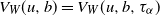
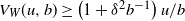
 \begin{align*}{V_W}(u,b,T) = E\left[ {\frac{{u + W(T)}}{{b + T}}} \right],\quad {V_W}(u,b) = \mathop {\sup }\limits_T {V_W}(u,b,T),\end{align*}
where u and b are real numbers with
 $b > 0$
. T being a stopping time means it is a non-negative real-valued random variable that does not anticipate the future, and the sup is taken over stopping times for which the expectation exists. Let
$b > 0$
. T being a stopping time means it is a non-negative real-valued random variable that does not anticipate the future, and the sup is taken over stopping times for which the expectation exists. Let
 $\alpha $
be the unique real root of
$\alpha $
be the unique real root of
 $\alpha = (1 - {\alpha ^2})\int_0^\infty {\exp \left( {\lambda \alpha - {\lambda ^2}/2} \right)d\lambda } $
. Computation gives
$\alpha = (1 - {\alpha ^2})\int_0^\infty {\exp \left( {\lambda \alpha - {\lambda ^2}/2} \right)d\lambda } $
. Computation gives
 $\alpha = 0.83992\ldots.$
Let
$\alpha = 0.83992\ldots.$
Let
 ${\tau _\alpha } = \min \left\{ {t:u + W(t) \ge \alpha \sqrt {b + t} } \right\}$
. They proved
${\tau _\alpha } = \min \left\{ {t:u + W(t) \ge \alpha \sqrt {b + t} } \right\}$
. They proved
 ${\tau _\alpha }$
is the almost surely unique optimal stopping time, so
${\tau _\alpha }$
is the almost surely unique optimal stopping time, so
 ${V_W}(u,b) = {V_W}(u,b,{\tau _\alpha })$
; and
${V_W}(u,b) = {V_W}(u,b,{\tau _\alpha })$
; and
 \begin{equation}{V_W}(u,b)=(1 - {\alpha ^2})\int_0^\infty {\exp \left( {\lambda u - {\lambda ^2}b/2} \right)d\lambda }\text{ if }u \le \alpha \sqrt b,\quad\text{else }{V_W}(u,b) = u/b.\end{equation}
In other words, starting at time b, it is optimal to stop when you hit the square root boundary
 $\alpha \sqrt {b + t} $
. Using the invariance principle (see, for example, [Reference Breiman1, p. 281]), Shepp [Reference Shepp13, pp. 1005–1006] used the Brownian motion result to show that the optimal stopping boundary for the random walk game is asymptotic to
$\alpha \sqrt {b + t} $
. Using the invariance principle (see, for example, [Reference Breiman1, p. 281]), Shepp [Reference Shepp13, pp. 1005–1006] used the Brownian motion result to show that the optimal stopping boundary for the random walk game is asymptotic to
 $\alpha \sqrt n $
; that is,
$\alpha \sqrt n $
; that is,
 $\mathop {\lim }_{n \to \infty } {\beta _n}/{\sqrt n} = \alpha$
. But that does not give a way of knowing if it is optimal to stop at any specific position (u,n) in the Chow–Robbins game, when u is an integer. Medina and Zeilberger [Reference Medina and Zeilberger10] discuss this distinction, pointing out that, at the time of their article (2009), not even
$\mathop {\lim }_{n \to \infty } {\beta _n}/{\sqrt n} = \alpha$
. But that does not give a way of knowing if it is optimal to stop at any specific position (u,n) in the Chow–Robbins game, when u is an integer. Medina and Zeilberger [Reference Medina and Zeilberger10] discuss this distinction, pointing out that, at the time of their article (2009), not even
 ${k_8}$
was known (they refer to it as
${k_8}$
was known (they refer to it as
 ${\beta _8}$
, but we are adopting the notation of the original papers). They give some numerical data about early positions, and some good insight into the difficulty.
${\beta _8}$
, but we are adopting the notation of the original papers). They give some numerical data about early positions, and some good insight into the difficulty.
In 2013, Häggström and Wästlund [Reference Dvoretzky6] showed, with a clever idea and the help of computer calculations, how to finesse the difficulty discussed in [Reference Medina and Zeilberger10], and actually decide in some ‘early’ positions whether or not stopping is optimal. Let d be the number of heads minus the number of tails after n flips. They expressed their results in terms of the number of heads, but we will give equivalent statements using n, to align with the usual notation. Also they expressed the stop rule in terms of n as a function of d, the reverse of the usual. We found it very useful in our numerical experiments below to also use this reverse formulation, so we describe it here. Using somewhat crude upper and lower bounds for the value at any position, and using backward induction from ‘way out’ (a horizon), they computed, for d between 1 and 25, numbers
 ${n_s}(d)$
and
${n_s}(d)$
and
 ${n_g}(d)$
, with
${n_g}(d)$
, with
 ${n_s}(d)<{n_g}(d)$
, such that if
${n_s}(d)<{n_g}(d)$
, such that if
 $n \le {n_s}(d)$
you should stop, and if
$n \le {n_s}(d)$
you should stop, and if
 $n \ge {n_g}(d)$
you should go on. The idea is that as you work backward from the horizon, those numbers should pull closer together. For d less than 12, and for several more ds between 13 and 25, for their horizon they found
$n \ge {n_g}(d)$
you should go on. The idea is that as you work backward from the horizon, those numbers should pull closer together. For d less than 12, and for several more ds between 13 and 25, for their horizon they found
 ${n_g}(d) = {n_s}(d) + 2$
(note that d and n have the same parity), in which case stopping if and only if
${n_g}(d) = {n_s}(d) + 2$
(note that d and n have the same parity), in which case stopping if and only if
 $n \le {n_s}(d)$
is the rigorous optimal stop rule for that d. Shepp’s asymptotic value for the stopping rule put in this reverse formulation is
$n \le {n_s}(d)$
is the rigorous optimal stop rule for that d. Shepp’s asymptotic value for the stopping rule put in this reverse formulation is
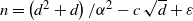
 ${n_s}(d) \cong {d^2}/{\alpha ^2}$
. This is not so accurate: if you look at just the few cases where Häggström and Wästlund actually find
${n_s}(d) \cong {d^2}/{\alpha ^2}$
. This is not so accurate: if you look at just the few cases where Häggström and Wästlund actually find
 ${n_s}(d)$
, you can already see that it is off about first order in d, and actually it appears that
${n_s}(d)$
, you can already see that it is off about first order in d, and actually it appears that
 ${n_s}(d) \cong ({d^2} + d)/{\alpha ^2}$
. Solving for d in terms of n, this is consistent with the suggestion by Lai, Yao, and Aitsahlia [Reference Leung Lai, Yao and Aitsahlia9, p. 768], that the stopping boundary for d in terms of n, should be
${n_s}(d) \cong ({d^2} + d)/{\alpha ^2}$
. Solving for d in terms of n, this is consistent with the suggestion by Lai, Yao, and Aitsahlia [Reference Leung Lai, Yao and Aitsahlia9, p. 768], that the stopping boundary for d in terms of n, should be
 ${\beta _n} = \alpha \sqrt n - 1/2 + o(1)$
.
${\beta _n} = \alpha \sqrt n - 1/2 + o(1)$
.
But this limited amount of numerical data is not able to suggest anything more. By having much better upper and lower bounds, it is possible to get much more data. Christensen and Fischer [Reference Christensen and Fischer5] (2022) gave much better upper and lower bounds for the optimal stopping value V for the random walk, and used it to numerically settle very many more cases. They found the stop rule for n up to 489 241, which corresponds to d up to about 588. We used the same upper bound that they did (with a different proof), but with a different lower bound, and settled yet again very many more cases than in [Reference Christensen and Fischer5], to attempt to get more numerical insight, as described in Section 1.3. This eventually led to using our bounds to prove the theoretical results which are the subject of this paper.
1.2. Embedding the random walk in Brownian motion, and Value bounds
Our proofs of the upper and lower bounds on V use the classical embedding of the random walk in W using first-exit times, due to A. V. Skorohod (see, for example, [Reference Breiman2, p. 293]), which make the results seem rather intuitive. The embedding idea is quite natural: simply sample the Brownian path each time it changes by
 $ \pm 1$
, and you get a version of the symmetric random walk. Formally, the properties follow from the strong Markov property. Let
$ \pm 1$
, and you get a version of the symmetric random walk. Formally, the properties follow from the strong Markov property. Let
 ${T_0} = 0,\,{T_n} = \min \left\{ {t > {T_{n - 1}}:|W(t) - W({T_{n - 1}})| = 1} \right\},n = 1,2,\ldots.$
Then
${T_0} = 0,\,{T_n} = \min \left\{ {t > {T_{n - 1}}:|W(t) - W({T_{n - 1}})| = 1} \right\},n = 1,2,\ldots.$
Then
 $W({T_n}),n = 0,1,\ldots,$
has the same distribution as the process
$W({T_n}),n = 0,1,\ldots,$
has the same distribution as the process
 ${S_n},n = 0,1,2,\ldots,$
and
${S_n},n = 0,1,2,\ldots,$
and
 $({T_n} - {T_{n - 1}},W({T_n}) - W({T_{n - 1}})),n = 1,2,\ldots,$
is an i.i.d. sequence, and
$({T_n} - {T_{n - 1}},W({T_n}) - W({T_{n - 1}})),n = 1,2,\ldots,$
is an i.i.d. sequence, and
 $E\left[ {{T_n}} \right] = n$
. Since the exit boundaries
$E\left[ {{T_n}} \right] = n$
. Since the exit boundaries
 $W({T_{n - 1}}) + 1,W({T_{n - 1}}) - 1$
are symmetric about
$W({T_{n - 1}}) + 1,W({T_{n - 1}}) - 1$
are symmetric about
 $W({T_{n - 1}})$
in this case, it can be shown that the sequence
$W({T_{n - 1}})$
in this case, it can be shown that the sequence
 ${T_1},{T_2},\ldots,{T_n},\ldots$
is independent from
${T_1},{T_2},\ldots,{T_n},\ldots$
is independent from
 $W({T_1}),W({T_2}),\ldots,W({T_n}),\ldots.$
Lemma 1.1. (Christensen and Fischer [Reference Christensen and Fischer5, Theorem 1, p. 3])
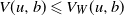 $V(u,b) \leqslant {V_W}(u,b)$
.
$V(u,b) \leqslant {V_W}(u,b)$
.
Proof. Their proof uses superharmonic functions, in a more general setting. We give a proof using the embedding idea, as a preliminary for using it in our lower bound proof. Let
 $n^*$
be a stopping time for
$n^*$
be a stopping time for
 ${S_n}$
. This induces a stopping time
${S_n}$
. This induces a stopping time
 $T^* = {T_{n^*}}$
on W. So
$T^* = {T_{n^*}}$
on W. So
 \begin{align*}{V_W}(u,b) \ge E\left[ {\frac{{u + W(T^*)}}{{b + T^*}}} \right] &= \sum\limits_{n = 0}^\infty {E\left[ {\left. {\frac{{u + W({T_n})}}{{b + {T_n}}}} \right|T^* = {T_n}} \right]} P(n^* = n)\\ &= \sum\limits_{n = 0}^\infty {E\left[ {\left. {\frac{{u + W({T_n})}}{{b + n}}\frac{{b + n}}{{b + {T_n}}}} \right|T^* = {T_n}} \right]} P(n^* = n).\end{align*}
But
 ${T_n}$
is independent of
${T_n}$
is independent of
 $W({T_n})$
, and is also independent of
$W({T_n})$
, and is also independent of
 ${I_{T^* = {T_n}}}$
since the latter is a function of
${I_{T^* = {T_n}}}$
since the latter is a function of
 $W({T_1}),W({T_2}),\ldots,W({T_n})$
, since
$W({T_1}),W({T_2}),\ldots,W({T_n})$
, since
 $T^*$
is a stopping time. Thus
$T^*$
is a stopping time. Thus
 $ E\left[ {\frac{{u + W(T^*)}}{{b + T^*}}} \right]= \sum\limits_{n = 0}^\infty {E\left[ {\frac{{b + n}}{{b + {T_n}}}} \right]E\left[ {\left. {\frac{{u + W({T_n})}}{{b + n}}} \right|T^* = {T_n}} \right]} P(n^* = n).$
By Jensen’s inequality,
$ E\left[ {\frac{{u + W(T^*)}}{{b + T^*}}} \right]= \sum\limits_{n = 0}^\infty {E\left[ {\frac{{b + n}}{{b + {T_n}}}} \right]E\left[ {\left. {\frac{{u + W({T_n})}}{{b + n}}} \right|T^* = {T_n}} \right]} P(n^* = n).$
By Jensen’s inequality,
 $E\left[ {\frac{{b + n}}{{b + {T_n}}}} \right] \ge \frac{{b + n}}{{E\left[ {b + {T_n}} \right]}} = 1,$
so
$E\left[ {\frac{{b + n}}{{b + {T_n}}}} \right] \ge \frac{{b + n}}{{E\left[ {b + {T_n}} \right]}} = 1,$
so
 \begin{align*}{V_W}(u,b) &\ge \sum\limits_{n = 0}^\infty {E\left[ {\left. {\frac{{u + W({T_n})}}{{b + n}}} \right|T^* = {T_n}} \right]} P(n^* = n)\\ &= \sum\limits_{n = 0}^\infty {E\left[ {\left. {\frac{{u + {S_n}}}{{b + n}}} \right|n^* = n} \right]} P(n^* = n)\\ &= E\left[ {\frac{{u + {S_{n^*}}}}{{b + n^*}}} \right] = V(u,b,n^*).\\[-30pt]\end{align*}
In retrospect, it is as one would think: the random walk is a just a sampling of the Brownian motion, so naturally it cannot do any better. There is the little matter of different denominators in the payoff, but Jensen’s inequality goes the right way for that. For a lower bound, we have the following result.
Lemma 1.2.
 \begin{align*}V(u,b) \ge {V_W}(u,b)\left( {1 - \frac{5}{{12b}}\left( {1 + \frac{1}{{\sqrt b }}} \right)} \right),\quad b > 1600.\end{align*}
We will give a detailed proof of Lemma 1.2 in Appendix A. But the idea for our proof of this lemma is simple enough. For u below the Brownian boundary, run the Brownian motion until it hits the nearest integer to
 $\alpha \sqrt {b + t} \,\,\, - u$
. With that stop rule,
$\alpha \sqrt {b + t} \,\,\, - u$
. With that stop rule,
 $E\left[ {\frac{{u + W(T)}}{{b + T}}} \right]$
is about the same as
$E\left[ {\frac{{u + W(T)}}{{b + T}}} \right]$
is about the same as
 ${V_W}(u,b)$
because we are so close to the boundary; we will quantify this using a modified fundamental Wald identity of Shepp to obtain
${V_W}(u,b)$
because we are so close to the boundary; we will quantify this using a modified fundamental Wald identity of Shepp to obtain
 $E\left[ {\frac{{u + W(T)}}{{b + T}}} \right] \ge {V_W}(u,b)\left( {1 - \frac{1}{{4b}}\left( {1 + \frac{1}{{\sqrt b }}} \right)} \right)$
. But W(T) is an integer, so in terms of the embedded random walk process
$E\left[ {\frac{{u + W(T)}}{{b + T}}} \right] \ge {V_W}(u,b)\left( {1 - \frac{1}{{4b}}\left( {1 + \frac{1}{{\sqrt b }}} \right)} \right)$
. But W(T) is an integer, so in terms of the embedded random walk process
 ${S_n} = W({T_n})$
,
${S_n} = W({T_n})$
,
 $E\left[ {\frac{{u + W(T)}}{{b + T}}} \right] = \sum_{n = 0}^\infty {E\left[ {\left. {\frac{{u + {S_n}}}{{b + {T_n}}}} \right|{n^*} = n} \right]} P({n^*} = n)$
. Proceed as in the proof of Lemma 1.1. Jensen’s inequality goes the wrong way this time; but knowing the moments of the random time differences of the embedding, we can show that
$E\left[ {\frac{{u + W(T)}}{{b + T}}} \right] = \sum_{n = 0}^\infty {E\left[ {\left. {\frac{{u + {S_n}}}{{b + {T_n}}}} \right|{n^*} = n} \right]} P({n^*} = n)$
. Proceed as in the proof of Lemma 1.1. Jensen’s inequality goes the wrong way this time; but knowing the moments of the random time differences of the embedding, we can show that
 $E\left[ {\frac{{b + n}}{{b + {T_n}}}} \right] \le \left( {1 + \frac{1}{{6b}}} \right)$
, so
$E\left[ {\frac{{b + n}}{{b + {T_n}}}} \right] \le \left( {1 + \frac{1}{{6b}}} \right)$
, so
 $E\left[ {\frac{{u + W(T)}}{{b + T}}} \right] \le \left( {1 + \frac{1}{{6b}}} \right)\sum_{n = 0}^\infty {E\left[ {\left. {\frac{{u + {S_n}}}{{b + n}}} \right|{n^*} = n} \right]} P({n^*} = n) = \left( {1 + \frac{1}{{6b}}} \right)V(u,b)$
, implying the lemma.
$E\left[ {\frac{{u + W(T)}}{{b + T}}} \right] \le \left( {1 + \frac{1}{{6b}}} \right)\sum_{n = 0}^\infty {E\left[ {\left. {\frac{{u + {S_n}}}{{b + n}}} \right|{n^*} = n} \right]} P({n^*} = n) = \left( {1 + \frac{1}{{6b}}} \right)V(u,b)$
, implying the lemma.
How good are these bounds? The data show, and we will prove later, that if integer u happens to be just a hair more than
 $\alpha \sqrt b - 1/2$
, then
$\alpha \sqrt b - 1/2$
, then
 $V(u,b) = u/b$
, but
$V(u,b) = u/b$
, but
 ${V_W}(u,b) \cong \left( {1 + 0.25{b^{ - 1}}} \right)u/b$
, so the Brownian upper bound overshoots the true value by a relative error of
${V_W}(u,b) \cong \left( {1 + 0.25{b^{ - 1}}} \right)u/b$
, so the Brownian upper bound overshoots the true value by a relative error of
 $O({b^{ - 1}})$
at some places, for arbitrarily large b. The same examples give
$O({b^{ - 1}})$
at some places, for arbitrarily large b. The same examples give
 $V(u,b) \cong {V_W}(u,b)\left( {1 - 0.25{b^{ - 1}}} \right)$
, so we cannot expect a lower bound of the form
$V(u,b) \cong {V_W}(u,b)\left( {1 - 0.25{b^{ - 1}}} \right)$
, so we cannot expect a lower bound of the form
 $V(u,b) \cong {V_W}(u,b)\left( {1 - c{b^{ - 1}}} \right)$
to do better than this. Lemma 1.2 gets lower bound
$V(u,b) \cong {V_W}(u,b)\left( {1 - c{b^{ - 1}}} \right)$
to do better than this. Lemma 1.2 gets lower bound
 $ {V_W}(u,b)\left( {1 - 0.42{b^{ - 1}}} \right)$
. Theorem 5.1 later will give a greatly improved approximation to V when u is near the boundary, showing that
$ {V_W}(u,b)\left( {1 - 0.42{b^{ - 1}}} \right)$
. Theorem 5.1 later will give a greatly improved approximation to V when u is near the boundary, showing that
 ${V_W}$
is off from the true V by essentially a relative error of
${V_W}$
is off from the true V by essentially a relative error of
 $0.25{b^{ - 1}}$
at half-integer values below the boundary, and the true V is approximately piecewise linear in between, when the distance below the boundary is not more than about
$0.25{b^{ - 1}}$
at half-integer values below the boundary, and the true V is approximately piecewise linear in between, when the distance below the boundary is not more than about
 ${b^{1/12}}$
. Theorem 5.1 does not give specific values for the constants (though that could be done with enough pain), and it was not used in our numerical work. Christensen and Fischer also give a lower bound, but our simple formula is convenient for our numerical work, and more importantly, for the later proof of the theoretical main results.
${b^{1/12}}$
. Theorem 5.1 does not give specific values for the constants (though that could be done with enough pain), and it was not used in our numerical work. Christensen and Fischer also give a lower bound, but our simple formula is convenient for our numerical work, and more importantly, for the later proof of the theoretical main results.
1.3. Numerical exploration and speculation
Using these good upper and lower bounds, we carried out the Häggström–Wästlund method numerically from a horizon of
 $n = {10^9}$
, and found
$n = {10^9}$
, and found
 ${n_g}(d) = {n_s}(d) + 2$
for d up to 7995, and almost all cases up to 20 000, so that the stop rule is settled for those. Stated another way, it settles all cases where
${n_g}(d) = {n_s}(d) + 2$
for d up to 7995, and almost all cases up to 20 000, so that the stop rule is settled for those. Stated another way, it settles all cases where
 $n < {7995^2}/{\alpha ^2} \cong 9 \times {10^7}$
, and most cases where
$n < {7995^2}/{\alpha ^2} \cong 9 \times {10^7}$
, and most cases where
 $n < {20\,000^2}/{\alpha ^2} \cong 5.7 \times {10^8}$
, over half a billion, going considerably beyond Christensen and Fischer. Our computations did not really take much computer time, and we could have gone a lot further, but we got pleasantly sidetracked by discovering the theoretical arguments of this paper. Having the stop-go boundaries as a function of d rather than n, following Häggström and Wästlund, made the computer algorithm extremely efficient and suitable for dealing with very large numbers. The spreadsheet for the answer has only 20 000 rows, rather than a billion. Figure 1 is a graph of
$n < {20\,000^2}/{\alpha ^2} \cong 5.7 \times {10^8}$
, over half a billion, going considerably beyond Christensen and Fischer. Our computations did not really take much computer time, and we could have gone a lot further, but we got pleasantly sidetracked by discovering the theoretical arguments of this paper. Having the stop-go boundaries as a function of d rather than n, following Häggström and Wästlund, made the computer algorithm extremely efficient and suitable for dealing with very large numbers. The spreadsheet for the answer has only 20 000 rows, rather than a billion. Figure 1 is a graph of
 ${n_g}(d) - \left( {{d^2} + d} \right)/{\alpha ^2}$
for d up to 20 000, from the spreadsheet; for almost all of those cases, and for all cases up to
${n_g}(d) - \left( {{d^2} + d} \right)/{\alpha ^2}$
for d up to 20 000, from the spreadsheet; for almost all of those cases, and for all cases up to
 $d = 7995$
,
$d = 7995$
,
 ${n_g}(d) = {n_s}(d) +2$
. It appears thick since it is oscillating with amplitude about 1 around a square root curve.
${n_g}(d) = {n_s}(d) +2$
. It appears thick since it is oscillating with amplitude about 1 around a square root curve.

Figure 1.
 ${n_g}(d) - \left( {{d^2} + d} \right)/{\alpha ^2}$
versus d,
${n_g}(d) - \left( {{d^2} + d} \right)/{\alpha ^2}$
versus d,
 $d \le 20\,000$
.
$d \le 20\,000$
.
We originally speculated that
 ${n_s}(d) \cong \left( {{d^2} + d} \right)/{\alpha ^2} - \,{\pi ^{ - 1/2}}\sqrt d \,\,\,\, + \,\,\varepsilon ,$
with
${n_s}(d) \cong \left( {{d^2} + d} \right)/{\alpha ^2} - \,{\pi ^{ - 1/2}}\sqrt d \,\,\,\, + \,\,\varepsilon ,$
with
 $\varepsilon$
wiggling around zero with amplitude about 1. But this coefficient of
$\varepsilon$
wiggling around zero with amplitude about 1. But this coefficient of
 $\sqrt d $
turns out to be wrong, by about 1%. Theorem 1.1 will prove that the correct coefficient is
$\sqrt d $
turns out to be wrong, by about 1%. Theorem 1.1 will prove that the correct coefficient is
 $ - {\pi ^{ - 1/2}}\left( { - 4\zeta (\! -1/2)/\alpha } \right)$
. Since
$ - {\pi ^{ - 1/2}}\left( { - 4\zeta (\! -1/2)/\alpha } \right)$
. Since
 $ - 4\zeta (\! -1/2)/\alpha = 0.990\ldots$
, nature had a laugh at us for jumping to conclusions! Figure 2 is the detail for the 100 points at the large d end of the curve, showing the oscillation.
$ - 4\zeta (\! -1/2)/\alpha = 0.990\ldots$
, nature had a laugh at us for jumping to conclusions! Figure 2 is the detail for the 100 points at the large d end of the curve, showing the oscillation.

Figure 2. Last 100 points in Figure 1; horizontal coordinates shown are
 $d - 19\,900$
.
$d - 19\,900$
.
We now have, from theory, the correct coefficient for the
 $\sqrt d $
term, but there is still something suggested by the numerics that the theory has not yet reached. Assume
$\sqrt d $
term, but there is still something suggested by the numerics that the theory has not yet reached. Assume
 $\varepsilon = O(1)$
. Using the binomial expansion, we can solve for d in
$\varepsilon = O(1)$
. Using the binomial expansion, we can solve for d in
 $n = \left( {{d^2} + d} \right)/{\alpha ^2} - c\,\sqrt d + \varepsilon $
, expressing the boundary in the more usual way with d as a function of n. With a little algebra one arrives at the following conjecture.
$n = \left( {{d^2} + d} \right)/{\alpha ^2} - c\,\sqrt d + \varepsilon $
, expressing the boundary in the more usual way with d as a function of n. With a little algebra one arrives at the following conjecture.
 \begin{equation}\text{Conjecture.} \quad{\beta _n} = \alpha \sqrt n \,\, - 1/2\,\, + \,\,\frac{{\left( { - 2\zeta ( \!- 1/2)} \right)\sqrt \alpha }}{{\sqrt \pi }}{n^{ - 1/4}} + O({n^{ - 1/2}}) \text{?}\end{equation}
Theorem 1.1 will prove that the coefficient of
 $n^{-1/4}$
is correct, but it will only get the error term to
$n^{-1/4}$
is correct, but it will only get the error term to
 $O\left(n^{-7/24}\right)$
. There is still theoretical work needed to catch up with the numerical speculation.
$O\left(n^{-7/24}\right)$
. There is still theoretical work needed to catch up with the numerical speculation.
Christensen and Fischer [Reference Christensen and Fischer5] had conjectured an
 ${n^{ - 1/4}}$
dependence, based on numerical evidence. They found that for n up to 489 241, the Chow–Robbins boundary is
${n^{ - 1/4}}$
dependence, based on numerical evidence. They found that for n up to 489 241, the Chow–Robbins boundary is
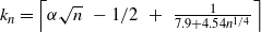 ${k_n} = \left\lceil {\alpha \sqrt n \,\, - 1/2\,\, + \,\,\frac{1}{{7.9 + 4.54{n^{1/4}}}}} \right\rceil $
except for eight stray ns in that range. Note that
${k_n} = \left\lceil {\alpha \sqrt n \,\, - 1/2\,\, + \,\,\frac{1}{{7.9 + 4.54{n^{1/4}}}}} \right\rceil $
except for eight stray ns in that range. Note that
 $\frac{1}{{4.54}} $
differs from
$\frac{1}{{4.54}} $
differs from
 $\frac{{\left( { - 2\zeta ( -1/2)} \right)\sqrt \alpha }}{{\sqrt \pi }}$
by about 2.5%.
$\frac{{\left( { - 2\zeta ( -1/2)} \right)\sqrt \alpha }}{{\sqrt \pi }}$
by about 2.5%.
Added after review. From recent numerical work after this paper was already refereed, we discovered a simple formula that gives the stop rule for all cases up to a quite large number. Let
 $p(d) = \left( {{d^2} + d} \right)/{\alpha ^2} - {\pi ^{ - 1/2}}\left( { - 4\zeta ( \!- 1/2)/\alpha } \right) \sqrt d -0.064\,998\,6 - 7/(d+95)$
. Then
$p(d) = \left( {{d^2} + d} \right)/{\alpha ^2} - {\pi ^{ - 1/2}}\left( { - 4\zeta ( \!- 1/2)/\alpha } \right) \sqrt d -0.064\,998\,6 - 7/(d+95)$
. Then
 \begin{align*}{n_s}(d) = \text{nearest integer to } p(d) \text{ that has the same parity as }d\end{align*}
gives the exact optimal stop rule for all d from 2 to 15 363 (which covers all n up to over a third of a billion). We had thought that the oscillatory behavior meant that finding a simple exact formula was unlikely, but now it appears that it could be merely nearest-integer behavior around an analytic asymptotic formula. For now, we have no idea how to get any such formula; the correction terms above were purely ad hoc.
1.4. Statement of main theorems
Using the idea of Häggström and Wästlund to use backward induction from a horizon, but proceeding algebraically rather than numerically, we will be led to a tree with weights corresponding to Catalan numbers and Shapiro Catalan triangle numbers, and a generalized backward induction principle. Before starting the development, we will state up front the main theorems that eventually follow from it. The second one is a corollary of the first, and gives a formula for the exact optimal stopping rule for the original Chow–Robbins game for all n, except in a set whose density goes to zero at the rate
 $O(n^{-7/24})$
. The longer the game goes on, the more likely it is that you will be able to stop optimally, and know that you did (from the description in Theorem 1.2). Actually, using the method of proof of Theorem 1.2, the estimate
$O(n^{-7/24})$
. The longer the game goes on, the more likely it is that you will be able to stop optimally, and know that you did (from the description in Theorem 1.2). Actually, using the method of proof of Theorem 1.2, the estimate
 ${\beta _n} = \alpha \sqrt n - 1/2 + o(1)$
suggested in [Reference Leung Lai, Yao and Aitsahlia9] already implies an exact stopping rule for all n except for a set of asymptotic density zero, although with no rate implied since there is no quantification of the o(1) term. We thank a referee for pointing that out. As far as we know, it had not been noticed before.
${\beta _n} = \alpha \sqrt n - 1/2 + o(1)$
suggested in [Reference Leung Lai, Yao and Aitsahlia9] already implies an exact stopping rule for all n except for a set of asymptotic density zero, although with no rate implied since there is no quantification of the o(1) term. We thank a referee for pointing that out. As far as we know, it had not been noticed before.
The Riemann zeta function
 $\zeta (\! - 1/2) = - 0.207\,886\ldots$
appears because the analysis in Section 6 involves the asymptotic approximation of the sum of square roots of the first k integers, the generalized harmonic number
$\zeta (\! - 1/2) = - 0.207\,886\ldots$
appears because the analysis in Section 6 involves the asymptotic approximation of the sum of square roots of the first k integers, the generalized harmonic number
 ${H_k}^{(\! -1/2)}$
.
${H_k}^{(\! -1/2)}$
.
Theorem 1.1.
 \begin{align*}{\beta _n} = \alpha \sqrt n \,\, - 1/2\,\, + \,\,\frac{{\left( { - 2\zeta ( \!- 1/2)} \right)\sqrt \alpha }}{{\sqrt \pi }}{n^{ - 1/4}} + O\left( {{n^{ - 7/24}}} \right).\end{align*}
Theorem 1.2.
 \begin{align*}{k_n} = \left\lceil {\alpha \sqrt n \,\, - 1/2\,\, + \,\,\frac{{\left( { - 2\zeta (\! - 1/2)} \right)\sqrt \alpha }}{{\sqrt \pi }}{n^{ - 1/4}}} \right\rceil, \end{align*}
except for a set S of integers for which
 $|S \cap \{1,\ldots,n\}|/n = O(n^{-7/24})$
. Specifically, there exists
$|S \cap \{1,\ldots,n\}|/n = O(n^{-7/24})$
. Specifically, there exists
 $A > 0$
and
$A > 0$
and
 ${n_0}$
such that for
${n_0}$
such that for
 $n \ge {n_0}$
, the given formula for
$n \ge {n_0}$
, the given formula for
 $k_n$
holds if
$k_n$
holds if
 \begin{align*}&\left\lceil {\alpha \sqrt n \,\, - 1/2\,\, + \,\,\frac{{\left( { - 2\zeta (\! -1/2)} \right)\sqrt \alpha }}{{\sqrt \pi }}{n^{ - 1/4}} - A{n^{ - 7/24}}} \right\rceil \\ &=\quad\left\lceil {\alpha \sqrt n \,\, - 1/2\,\, + \,\,\frac{{\left( { - 2\zeta (\! -1/2)} \right)\sqrt \alpha }}{{\sqrt \pi }}{n^{ - 1/4}} + A{n^{ - 7/24}}} \right\rceil.\end{align*}
Proof. Figure 3 shows how Theorem 1.2 follows easily from Theorem 1.1. Let
 \begin{align*}{f_1}(n) = \alpha \sqrt n \,\, - 1/2\,\, + \,\,\frac{{\left( { - 2\zeta (\! -1/2)} \right)\sqrt \alpha }}{{\sqrt \pi }}{n^{ - 1/4}} - A{n^{ - 7/24}},\\{f_2}(n) = \alpha \sqrt n \,\, - 1/2\,\, + \,\,\frac{{\left( { - 2\zeta (\! -1/2)} \right)\sqrt \alpha }}{{\sqrt \pi }}{n^{ - 1/4}} + A{n^{ - 7/24}},\end{align*}
with A chosen according to Theorem 1.1 so that
 ${f_1}(n) < {\beta _n} < {f_2}(n)$
for all
${f_1}(n) < {\beta _n} < {f_2}(n)$
for all
 $n \ge {n_0}$
. Let u be a positive integer, and let
$n \ge {n_0}$
. Let u be a positive integer, and let
 ${n_1},{n_2},{n_3}$
satisfy
${n_1},{n_2},{n_3}$
satisfy
 ${f_2}({n_1}) = u,{f_1}({n_2}) = u,{f_2}({n_3}) = u + 1$
, where for this purpose we extend the domain of
${f_2}({n_1}) = u,{f_1}({n_2}) = u,{f_2}({n_3}) = u + 1$
, where for this purpose we extend the domain of
 ${f_1},{f_2}$
so that
${f_1},{f_2}$
so that
 ${n_1},{n_2},{n_3}$
are real, not necessarily integers. Assume also that u is large enough so that
${n_1},{n_2},{n_3}$
are real, not necessarily integers. Assume also that u is large enough so that
 ${n_1} \ge {n_0}$
.
${n_1} \ge {n_0}$
.

Figure 3. Graph of
 ${f_1}(n)$
and
${f_1}(n)$
and
 ${f_2}(n)$
.
${f_2}(n)$
.
 ${\beta _n}$
is somewhere between them, shown dotted.
${\beta _n}$
is somewhere between them, shown dotted.
For
 ${n_1} \le n \le {n_3}$
,
${n_1} \le n \le {n_3}$
,
 $\left\lceil {{f_1}(n)} \right\rceil = \left\lceil {{f_2}(n)} \right\rceil $
implies
$\left\lceil {{f_1}(n)} \right\rceil = \left\lceil {{f_2}(n)} \right\rceil $
implies
 ${n_2} \le n \le {n_3}$
. For integers n such that
${n_2} \le n \le {n_3}$
. For integers n such that
 ${n_2} \le n \le {n_3}$
, we have
${n_2} \le n \le {n_3}$
, we have
 $u < {\beta _n} < u + 1$
, so it is optimal to stop at
$u < {\beta _n} < u + 1$
, so it is optimal to stop at
 $u + 1$
, and for those integers
$u + 1$
, and for those integers
 ${k_n} = u + 1 = \left\lceil {\alpha \sqrt n \,\, - 1/2\,\, + \,\,\dfrac{{\left( { - 2\zeta (\! -1/2)} \right)\sqrt \alpha }}{{\sqrt \pi }}{n^{ - 1/4}}} \right\rceil.$
We are uncertain of the stop rule in the interval
${k_n} = u + 1 = \left\lceil {\alpha \sqrt n \,\, - 1/2\,\, + \,\,\dfrac{{\left( { - 2\zeta (\! -1/2)} \right)\sqrt \alpha }}{{\sqrt \pi }}{n^{ - 1/4}}} \right\rceil.$
We are uncertain of the stop rule in the interval
 $\left[ {{n_1},{n_2}} \right]$
, and S is contained in the union of those. By the mean value theorem,
$\left[ {{n_1},{n_2}} \right]$
, and S is contained in the union of those. By the mean value theorem,
 $f_2(n_2) - f_1(n_2) = f_2'(n*)(n_2 - n_1)$
for some
$f_2(n_2) - f_1(n_2) = f_2'(n*)(n_2 - n_1)$
for some
 $n_1 < n* < n_2$
, and
$n_1 < n* < n_2$
, and
 $f_2'(n*) \ge f_2'(n_2) = \alpha n_2^{-1/2}/2 -o(n^{-1/2}) > n_2^{-1/2}/2$
for
$f_2'(n*) \ge f_2'(n_2) = \alpha n_2^{-1/2}/2 -o(n^{-1/2}) > n_2^{-1/2}/2$
for
 $n_2$
large, so
$n_2$
large, so
 $n_2 - n_1 < A{n_2^{-7/24}}/{n_2^{-1/2}} = O(n_2^{5/24}) = O(u^{5/12})$
. For the intervals
$n_2 - n_1 < A{n_2^{-7/24}}/{n_2^{-1/2}} = O(n_2^{5/24}) = O(u^{5/12})$
. For the intervals
 $\left[ {{n_1},{n_2}} \right]$
contained in
$\left[ {{n_1},{n_2}} \right]$
contained in
 $\{1,\ldots,n\}$
, we have
$\{1,\ldots,n\}$
, we have
 $u \le \alpha \sqrt{n}$
. So
$u \le \alpha \sqrt{n}$
. So
 $|S \cap \{1,\ldots,n\}|/n = O({\sum_{u=1}^{\alpha\sqrt{n}} u^{5/12}}/n) = O(n^{-7/24})$
.
$|S \cap \{1,\ldots,n\}|/n = O({\sum_{u=1}^{\alpha\sqrt{n}} u^{5/12}}/n) = O(n^{-7/24})$
.
The set where we are uncertain has a simple description as a union of intervals
 $\left[ {{n_1},{n_2}} \right]$
pictured above. The ith such interval is centered halfway between where
$\left[ {{n_1},{n_2}} \right]$
pictured above. The ith such interval is centered halfway between where
 ${f_1}$
and
${f_1}$
and
 ${f_2}$
cross the horizontal line of height i, which is approximately at
${f_2}$
cross the horizontal line of height i, which is approximately at
 ${i^2}/{\alpha ^2}$
. The space between the ith and
${i^2}/{\alpha ^2}$
. The space between the ith and
 ${(i + 1)}$
th interval is
${(i + 1)}$
th interval is
 $O\left( i \right)$
. The length of the ith interval is
$O\left( i \right)$
. The length of the ith interval is
 $O\left( {{i^{5/12}}} \right)$
; if our speculation (1.2) were true, this length would be bounded. We have not given a specific numerical value for A, though it could be done. We resorted to expressing results in big-O notation, in spite of originally hoping not to do that, wanting results that are usable for computer exploration. But the calculations in later sections became too onerous.
$O\left( {{i^{5/12}}} \right)$
; if our speculation (1.2) were true, this length would be bounded. We have not given a specific numerical value for A, though it could be done. We resorted to expressing results in big-O notation, in spite of originally hoping not to do that, wanting results that are usable for computer exploration. But the calculations in later sections became too onerous.
The goal of the rest of this paper is to prove Theorem 1.1, by using a direct combinatorial assault going backwards in a tree. It is the Shapiro Catalan triangle properties that come to the rescue. Having gotten this far, we are more optimistic than Medina and Zeilberger [Reference Medina and Zeilberger10] about whether it is possible to get a formula for
 ${k_n}$
for all n. Conjecture (1.2) is possibly provable with refinements of the techniques in this paper, or something similar.
${k_n}$
for all n. Conjecture (1.2) is possibly provable with refinements of the techniques in this paper, or something similar.
Added after review: And the recently discovered formula given above at the end of Section 1.3 makes us yet more optimistic about the existence of a simple formula that works for all cases.
2. Generalized backward induction and the Shapiro Catalan triangle; plan for the proof of Theorem 1.1
We start by patiently wading through some backward induction steps, rewarding us with a recognized pattern. We will want to decide whether to stop or continue when u is below and near the Brownian boundary. Since we will be using the Brownian motion value function heavily for everything that follows, we switch back to using (u,b) for position, as Shepp did in his wonderful paper [Reference Shepp13] which inspired our theoretical work on bounds. We remark again that in our development from now on, u is real, not just an integer, even though the Chow–Robbins game itself has only integer values for positions. This is important because our analysis depends on approximating V(u,b) which is continuous in u. The graphs in Section 1.4 suggest the advantage of extending to the real case to do the analysis.
The famous backward induction principle of optimal stopping (see, for example, [Reference Chow, Robbins and Siegmund3]) applied to this simple random walk is
 \begin{align}&V(u,b) = \max \left\{ {\frac{u}{b},\frac{1}{2}V(u + 1,b + 1) + \frac{1}{2}V(u - 1,b + 1)} \right\}.\\&\text{Do not stop if }\frac{1}{2}V(u + 1,b + 1) + \frac{1}{2}V(u - 1,b + 1) > \frac{u}{b}; \quad\text{stop otherwise.} \nonumber\end{align}
This is the starting point for everything. Let us use it to get a preliminary result. Numerical evidence showed that if
 $\delta = \alpha \sqrt b \,\, - \,\,u$
is larger than 1/2 minus a hair (the hair being of the order of
$\delta = \alpha \sqrt b \,\, - \,\,u$
is larger than 1/2 minus a hair (the hair being of the order of
 ${b^{ - 1/4}}$
), you should not stop. Our bounds on V are not alone good enough to prove that without any backward steps, but let us see what we get that way. Using only our lower bound from Lemma 1.2 (assuming
${b^{ - 1/4}}$
), you should not stop. Our bounds on V are not alone good enough to prove that without any backward steps, but let us see what we get that way. Using only our lower bound from Lemma 1.2 (assuming
 $b > 1600$
), and a differential approximation
$b > 1600$
), and a differential approximation
 ${V_W}(u,b) \ge \left( {1 + {\delta ^2}{b^{ - 1}}} \right)u/b$
(from (3.6) in the next section), we get
${V_W}(u,b) \ge \left( {1 + {\delta ^2}{b^{ - 1}}} \right)u/b$
(from (3.6) in the next section), we get
 $V(u,b) \ge {V_W}(u,b)\left( {1 - 0.43{b^{ - 1}}} \right) \ge \left( {1 + {\delta ^2}{b^{ - 1}}} \right)\left( {1 - 0.43{b^{ - 1}}} \right)u/b$
, and this is greater than
$V(u,b) \ge {V_W}(u,b)\left( {1 - 0.43{b^{ - 1}}} \right) \ge \left( {1 + {\delta ^2}{b^{ - 1}}} \right)\left( {1 - 0.43{b^{ - 1}}} \right)u/b$
, and this is greater than
 $u/b$
if
$u/b$
if
 $\delta > 0.66$
. Well, that is something: continue if
$\delta > 0.66$
. Well, that is something: continue if
 $\delta > 0.66$
. But just one step of backward induction with our lower bound will show how it begins to close in on 1/2. The distance of
$\delta > 0.66$
. But just one step of backward induction with our lower bound will show how it begins to close in on 1/2. The distance of
 $u - 1$
from the Brownian boundary is
$u - 1$
from the Brownian boundary is
 $\alpha \sqrt {b + 1} \,\, - \,\,(u - 1) = \alpha \sqrt b + h - u + 1 = \delta + 1 + h$
, where
$\alpha \sqrt {b + 1} \,\, - \,\,(u - 1) = \alpha \sqrt b + h - u + 1 = \delta + 1 + h$
, where
 $0 < h < \alpha {b^{ - 1/2}}/2$
. So
$0 < h < \alpha {b^{ - 1/2}}/2$
. So
 \begin{align*}\frac{1}{2}V(u + 1,b + 1) + \frac{1}{2}V(u - 1,b + 1) &\geqslant \frac{1}{2}\frac{{u + 1}}{{b + 1}} + \frac{1}{2}{V_W}(u - 1,b + 1)\left( {1 - \frac{{0.43}}{{b + 1}}} \right)\\ &\geqslant \frac{1}{2}\frac{{u + 1}}{{b + 1}} + \frac{1}{2}\frac{{u - 1}}{{b + 1}}\left( {1 + \frac{{{{(1 + \delta )}^2}}}{{b + 1}}} \right)\left( {1 - \frac{{0.43}}{{b + 1}}} \right)\\ &= \frac{u}{b} - \frac{u}{{b(b + 1)}} \\&+ \frac{1}{2}\frac{{u\left( {1 - \frac{1}{{\alpha \sqrt b - \delta }}} \right)}}{{{{\left( {b + 1} \right)}^2}}}\!\left(\! {{{(1 + \delta )}^2} - 0.43 - \frac{{0.43{{(1 + \delta )}^2}}}{{b + 1}}} \right).\end{align*}
For sufficiently large b, so that we can throw out small stuff, the condition for this to be greater than
 $u/b$
is clearly
$u/b$
is clearly
 ${(1 + \delta )^2} - 0.43 > 2$
, or
${(1 + \delta )^2} - 0.43 > 2$
, or
 $\delta > 0.56$
. But to be concrete, assume
$\delta > 0.56$
. But to be concrete, assume
 $b > 1600$
and
$b > 1600$
and
 $u = \alpha \sqrt b \,\, - \delta \,\, > \alpha \sqrt b \,\, - 0.66$
(we already know to continue if
$u = \alpha \sqrt b \,\, - \delta \,\, > \alpha \sqrt b \,\, - 0.66$
(we already know to continue if
 $\delta $
greater than 0.66). Then some arithmetic shows that
$\delta $
greater than 0.66). Then some arithmetic shows that
 $\delta > 0.58$
is sufficient. That is an improvement. And we could go more steps back and get a better go bound.
$\delta > 0.58$
is sufficient. That is an improvement. And we could go more steps back and get a better go bound.
Similarly, we can use our upper bound and close in on 1/2 from above, and it is convenient to do one step of that, to get a preliminary stop bound, to avoid annoyances later. Stop if
 $(V(u + 1,b + 1) + V(u - 1,b + 1))/2 < u/b$
. And
$(V(u + 1,b + 1) + V(u - 1,b + 1))/2 < u/b$
. And
 $\alpha \sqrt {b + 1} \,\, - \,\,(u - 1) = \delta + 1 + h$
where h is as before. Looking ahead to (3.5) of the next section,
$\alpha \sqrt {b + 1} \,\, - \,\,(u - 1) = \delta + 1 + h$
where h is as before. Looking ahead to (3.5) of the next section,
 ${V_W}(u,b) \le u/b + \alpha {\delta ^2}{b^{ - 3/2}}$
. We have
${V_W}(u,b) \le u/b + \alpha {\delta ^2}{b^{ - 3/2}}$
. We have
 \begin{align*}\frac{1}{2}V(u + 1,b + 1) + \frac{1}{2}V(u - 1,b + 1) &\leqslant \frac{1}{2}\frac{{u + 1}}{{b + 1}} + \frac{1}{2}\left( {\frac{{u - 1}}{{b + 1}} + \alpha \frac{{{{(1 + \delta + h)}^2}}}{{{{\left( {b + 1} \right)}^{3/2}}}}} \right)\\ &= \frac{u}{b} - \frac{u}{{b(b + 1)}} + \frac{1}{2}\alpha \frac{{{{(1 + \delta + h)}^2}}}{{{{\left( {b + 1} \right)}^{3/2}}}}\\ &= \frac{u}{b} - \frac{{\alpha \sqrt b - \delta }}{{b(b + 1)}} + \frac{1}{2}\alpha \frac{{{{(1 + \delta + h)}^2}}}{{{{\left( {b + 1} \right)}^{3/2}}}}.\end{align*}
For sufficiently large b, the condition for this to be less than
 $u/b$
is clearly
$u/b$
is clearly
 ${(1 + \delta )^2} < 2$
, or
${(1 + \delta )^2} < 2$
, or
 $\delta < 0.414$
. But again to be concrete, assuming
$\delta < 0.414$
. But again to be concrete, assuming
 $b > 1600$
,
$b > 1600$
,
 $\delta < 0.38$
can be shown to be sufficient.
$\delta < 0.38$
can be shown to be sufficient.
With just one step of backward induction, we have already narrowed the range for the stopping boundary and proved the following lemma.
Lemma 2.1. For
 $b > 1600$
,
$b > 1600$
,
 $\alpha \sqrt b - 0.58 < {\beta _b} < \alpha \sqrt b - 0.38$
. Go if
$\alpha \sqrt b - 0.58 < {\beta _b} < \alpha \sqrt b - 0.38$
. Go if
 $\delta > 0.58$
, stop if
$\delta > 0.58$
, stop if
 $\delta < 0.38.$
This will be useful later, so it is noted. But the goal is to get to
 $\alpha \sqrt b - 1/2 + c{b^{ - 1/4}} + o({b^{ - 1/4}})$
, by continuing way down the backward induction tree.
$\alpha \sqrt b - 1/2 + c{b^{ - 1/4}} + o({b^{ - 1/4}})$
, by continuing way down the backward induction tree.
We proceed to systematize going backward. Continued backward induction leads to the tree in Figure 4, where further branching is stopped at
 $u + 1$
, creating leaves of the tree at those nodes, which are shown boxed. The V value at a node of the tree is greater than or equal to the average of the V values at its two parents. Figure 4 is a picture of eight rows of the backward induction tree. The meaning of the coefficients (weights) will be explained shortly, though it is perhaps already obvious from the way backward induction works for this simple symmetric random walk.
$u + 1$
, creating leaves of the tree at those nodes, which are shown boxed. The V value at a node of the tree is greater than or equal to the average of the V values at its two parents. Figure 4 is a picture of eight rows of the backward induction tree. The meaning of the coefficients (weights) will be explained shortly, though it is perhaps already obvious from the way backward induction works for this simple symmetric random walk.

Figure 4. Backward induction tree, with leaves boxed.
To explain the coefficients (the weights) displayed in Figure 4, consider the following succession of inequalities, using only the basic backward induction inequality (2.1):
 \begin{align*}&V(u,b) \geqslant \frac{1}{2}V(u + 1,b + 1) + \frac{1}{2}V(u - 1,b + 1),\\&\frac{1}{2}V(u - 1,b + 1) \geqslant \frac{1}{4}V(u,b + 2) + \frac{1}{4}V(u - 2,b + 2),\\&\frac{1}{4}V(u,b + 2) + \frac{1}{4}V(u - 2,b + 2)\\&\quad\geqslant \frac{1}{8}V(u + 1,b + 3) + \frac{1}{8}V(u - 1,b + 3) + \frac{1}{8}V(u - 1,b + 3) + \frac{1}{8}V(u - 3,b + 3)\\&\quad= \frac{1}{8}V(u + 1,b + 3) + \frac{2}{8}V(u - 1,b + 3) + \frac{1}{8}V(u - 3,b + 3),\\&\frac{2}{8}V(u - 1,b + 3) + \frac{1}{8}V(u - 3,b + 3)\\&\quad\geqslant \frac{2}{{16}}V(u,b + 4) + \frac{2}{{16}}V(u - 2,b + 4) + \frac{1}{{16}}V(u - 2,b + 4) + \frac{1}{6}V(u - 4,b + 4)\\&\quad= \frac{2}{{16}}V(u,b + 4) + \frac{3}{{16}}V(u - 2,b + 4) + \frac{1}{6}V(u - 4,b + 4),\\\ldots.\\\end{align*}
That is how the weights are generated, recursively. Considering any row of the tree, V(u,b) is greater than or equal to the sum of the weights times values at the leaves at or above that row, plus the weights times values at the non-leaf nodes at that row. The picture shows the weights through row 7, with the initial node at row 0. We were patient enough to carry out the trivial calculations by hand through seven rows, at which point we recognized the leaf weight numerators as being the Catalan numbers.
Now formalize the notation and the recursion. First, look at the nodes that are not leaves. With m indicating row number starting from 0 and j column number starting from 0 in the tree, let T(m,j) be the coefficient of
 ${2^{ - m}}V(u - j,b + m),m \geqslant 0,0 \leqslant j \leqslant m$
, and
${2^{ - m}}V(u - j,b + m),m \geqslant 0,0 \leqslant j \leqslant m$
, and
 $T(m,j) = 0$
outside this range. The initial condition is
$T(m,j) = 0$
outside this range. The initial condition is
 $T(0,0) = 1$
. The recursion
$T(0,0) = 1$
. The recursion
 $T(m,j) = T(m - 1,j - 1) + T(m - 1,j + 1)$
follows purely from backward induction. Using this recursion produces the table in Figure 5, through
$T(m,j) = T(m - 1,j - 1) + T(m - 1,j + 1)$
follows purely from backward induction. Using this recursion produces the table in Figure 5, through
 $m = 7$
.
$m = 7$
.

Figure 5. T(m,j), coefficient numerator in row m, col. j of tree in Figure 4.
In what follows we will only make use of the odd rows and columns of the tree in Figure 4, which correspond to the rows of the tree with leaves. Let
 $B(n,k) = T(2n - 1,2k - 1),n \ge 1,k \ge 1$
; Figure 6 shows the first four rows of B. The recursion for T implies (in two steps) the following recursion for B:
$B(n,k) = T(2n - 1,2k - 1),n \ge 1,k \ge 1$
; Figure 6 shows the first four rows of B. The recursion for T implies (in two steps) the following recursion for B:
 $B(n,k) = B(n - 1,k - 1) + 2B(n - 1,k) + B(n - 1,k + 1),n \ge 2,k \ge 2$
, with initial conditions
$B(n,k) = B(n - 1,k - 1) + 2B(n - 1,k) + B(n - 1,k + 1),n \ge 2,k \ge 2$
, with initial conditions
 $B(1,1) = 1$
and
$B(1,1) = 1$
and
 $B(1,k) = 0,k > 1$
. This is the recursion and initial conditions for the Shapiro Catalan triangle [Reference Shapiro12], one of the many arrays referred to in the literature as a Catalan triangle, or unfortunately sometimes as ‘the’ Catalan triangle. The columns of B (omitting the leading zeros) appear as every other diagonal in another popular ‘Catalan’s triangle’, the one that appears, for example, in the Wikipedia article of that name, which gives references to the history. But we need to reference our tree by row and column indices, so B is the right one for us. Fortunately, Miana and Romero [Reference Miana and Romero11] have the row moments for B (see (4.2)), which is exactly what we need for our purposes.
$B(1,k) = 0,k > 1$
. This is the recursion and initial conditions for the Shapiro Catalan triangle [Reference Shapiro12], one of the many arrays referred to in the literature as a Catalan triangle, or unfortunately sometimes as ‘the’ Catalan triangle. The columns of B (omitting the leading zeros) appear as every other diagonal in another popular ‘Catalan’s triangle’, the one that appears, for example, in the Wikipedia article of that name, which gives references to the history. But we need to reference our tree by row and column indices, so B is the right one for us. Fortunately, Miana and Romero [Reference Miana and Romero11] have the row moments for B (see (4.2)), which is exactly what we need for our purposes.

Figure 6. B(n,k), the odd rows and columns of T; it is the Shapiro Catalan triangle.
We now have a formula for the coefficients of the non-leaves in the odd rows of our backward induction tree in terms of well-known numbers:
 \begin{equation}{\textrm{coefficient of }}\,V(u - 2j + 1,b + 2m - 1) = {2^{ - 2m + 1}}B(m,j),\quad m \ge 1,j \ge 1.\end{equation}
There are simple known formulas for the entries in B:
 \begin{align*}B(m,j) = \frac{j}{m}\left( {\begin{array}{*{20}{c}} {2m} \\ {m - j}\end{array}} \right) = \left( {\begin{array}{*{20}{c}} {2m - 1} \\ {m - j}\end{array}} \right) - \left( {\begin{array}{*{20}{c}} {2m - 1} \\ {m - j - 1}\end{array}} \right).\end{align*}
The first column is
 \begin{align*}B(m,1) = \frac{1}{m}\left( {\begin{array}{*{20}{c}} {2m} \\ {m - 1}\end{array}} \right) = \frac{1}{{m + 1}}\left( {\begin{array}{*{20}{c}} {2m} \\ m\end{array}} \right) = \left( {\begin{array}{*{20}{c}} {2m - 1} \\ {m - 1}\end{array}} \right) - \left( {\begin{array}{*{20}{c}} {2m - 1} \\ {m - 2}\end{array}} \right) = {C_m}, \quad m \geqslant 1,\end{align*}
recognized as the mth Catalan number.
 ${C_0} = 1$
by definition.
${C_0} = 1$
by definition.
For the leaves, let L(n) be the coefficient of
 ${2^{ - 2n + 1}}V(u + 1,b + 2n - 1),n \ge 1$
, where
${2^{ - 2n + 1}}V(u + 1,b + 2n - 1),n \ge 1$
, where
 $n = 1,2,3,4,\ldots$
corresponds to rows
$n = 1,2,3,4,\ldots$
corresponds to rows
 $1,3,5,7,\ldots$
of the tree of Figure 4. The first four values of L(n) are 1,1,2,5, and from the way the tree is built, it is seen that
$1,3,5,7,\ldots$
of the tree of Figure 4. The first four values of L(n) are 1,1,2,5, and from the way the tree is built, it is seen that
 $L(n) = T(2n - 2,0) = T(2n - 3,1),n \ge 2$
, with
$L(n) = T(2n - 2,0) = T(2n - 3,1),n \ge 2$
, with
 $L(1) = 1$
. But
$L(1) = 1$
. But
 $T(2n - 3,1) = B(n - 1,1) = {C_{n - 1}}$
for
$T(2n - 3,1) = B(n - 1,1) = {C_{n - 1}}$
for
 $n \ge 2$
. So, we have the following formula for the leaf weights:
$n \ge 2$
. So, we have the following formula for the leaf weights:
 \begin{equation}{\text{coefficient of }}\,V(u + 1,b + 2n - 1) = {2^{ - 2n + 1}}{C_{n - 1}},\quad n \geqslant 1.\end{equation}
Returning to the inequality we started with, for any row, V(u,b) is greater than or equal to the sum of the weights times values at the leaves at or above that row, plus the weights times values at the non-leaf nodes in that row. Looking at only odd rows of the tree, for
 $n \ge 1$
, let
$n \ge 1$
, let
 \begin{align*}{S_L(n,u,b)} \,:\!= \sum\limits_{m = 0}^{n - 1} {{2^{ - 2m - 1}}{C_m}} V(u + 1,b + 2m + 1),\end{align*}
the sum of the leaves down through the row indexed by n; and
 \begin{align*}{S_R}(n,u,b) \,:\!= {2^{ - 2n + 1}}\sum\limits_{j = 1}^n {B(n,j)V(u - 2j + 1,b + 2n - 1)},\end{align*}
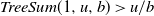
the sum of the non-leaves across the row indexed by n (an odd row of the original tree). Define
 \begin{equation}TreeSum(n,u,b) \,:\!= S_L(n,u,b) + {S_R}(n,u,b).\end{equation}
Thus for any
 $n \ge 1$
,
$n \ge 1$
,
 $V(u,b) \ge TreeSum(n,u,b)$
. This inequality is the summary of the chain of inequalities from repeated backward induction.
$V(u,b) \ge TreeSum(n,u,b)$
. This inequality is the summary of the chain of inequalities from repeated backward induction.
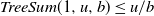
One property of TreeSum(n,u,b) is immediate from the basic backward induction principle (2.1):
 $TreeSum(n + 1,u,b) \le TreeSum(n,u,b),\,\,n \ge 1$
, which implies
$TreeSum(n + 1,u,b) \le TreeSum(n,u,b),\,\,n \ge 1$
, which implies
 $TreeSum(n,u,b) \le TreeSum(1,u,b) = \left( {V(u + 1,b + 1) + V(u - 1,b + 1)} \right)/2$
. Thus for any n,
$TreeSum(n,u,b) \le TreeSum(1,u,b) = \left( {V(u + 1,b + 1) + V(u - 1,b + 1)} \right)/2$
. Thus for any n,
 $TreeSum(n,u,b) > u/b \Rightarrow TreeSum(1,u,b) > u/b \Rightarrow V(u,b) > u/b$
, so do not stop at (u,b). To prove the other direction, let
$TreeSum(n,u,b) > u/b \Rightarrow TreeSum(1,u,b) > u/b \Rightarrow V(u,b) > u/b$
, so do not stop at (u,b). To prove the other direction, let
 $j \ge 0, k \ge 0$
.
$j \ge 0, k \ge 0$
.
 $V(u,b) > u/b \Rightarrow V(u-j,b) > (u-j)/b$
is obvious. Then
$V(u,b) > u/b \Rightarrow V(u-j,b) > (u-j)/b$
is obvious. Then
 $V(u-j,b) > (u-j)/b \Rightarrow u-j < {\beta}_b \Rightarrow u-b < {\beta}_{b+k}$
, from the monotonicity of Dvoretzky’s stop rules [Reference Dvoretzky6], so
$V(u-j,b) > (u-j)/b \Rightarrow u-j < {\beta}_b \Rightarrow u-b < {\beta}_{b+k}$
, from the monotonicity of Dvoretzky’s stop rules [Reference Dvoretzky6], so
 $V(u-j,b+k) > (u-j)/(b+k)$
. In other words, if you should not stop at (u,b), then you should not stop for a smaller u or a larger b. This implies that if
$V(u-j,b+k) > (u-j)/(b+k)$
. In other words, if you should not stop at (u,b), then you should not stop for a smaller u or a larger b. This implies that if
 $TreeSum(1,u,b) > u/b$
, then at every non-leaf node of the backward induction tree, the average of the values of its two children is greater than the ratio, so
$TreeSum(1,u,b) > u/b$
, then at every non-leaf node of the backward induction tree, the average of the values of its two children is greater than the ratio, so
 $TreeSum(n,u,b) = TreeSum(1,u,b)$
and
$TreeSum(n,u,b) = TreeSum(1,u,b)$
and
 $TreeSum(n,u,b) > u/b$
. This leads to the following lemma.
$TreeSum(n,u,b) > u/b$
. This leads to the following lemma.
Lemma 2.2. (Extended backward induction principle). Let
 $n \ge 1$
. Then
$n \ge 1$
. Then
 $V(u,b) = \max \left\{ {u/b,TreeSum(n,u,b)} \right\}$
; stop at (u,b) if
$V(u,b) = \max \left\{ {u/b,TreeSum(n,u,b)} \right\}$
; stop at (u,b) if
 $TreeSum(n,u,b) \le u/b$
, else continue.
$TreeSum(n,u,b) \le u/b$
, else continue.
 $TreeSum(1,u,b) > u/b \Rightarrow TreeSum(1,u,b) = TreeSum(n,u,b)$
.
$TreeSum(1,u,b) > u/b \Rightarrow TreeSum(1,u,b) = TreeSum(n,u,b)$
.
Proof. From the previous paragraph,
 $TreeSum(n,u,b) > u/b \Rightarrow TreeSum(1,u,b) > u/b$
which implies
$TreeSum(n,u,b) > u/b \Rightarrow TreeSum(1,u,b) > u/b$
which implies
 $TreeSum(n,u,b) = TreeSum(1,u,b) = V(u,b)$
. Now suppose
$TreeSum(n,u,b) = TreeSum(1,u,b) = V(u,b)$
. Now suppose
 $TreeSum(n,u,b) \le u/b$
. If
$TreeSum(n,u,b) \le u/b$
. If
 $TreeSum(1,u,b) > u/b$
, then by the previous paragraph,
$TreeSum(1,u,b) > u/b$
, then by the previous paragraph,
 $TreeSum(n,u,b) = TreeSum(1,u,b) > u/b$
, a contradiction. So
$TreeSum(n,u,b) = TreeSum(1,u,b) > u/b$
, a contradiction. So
 $TreeSum(1,u,b) \le u/b$
, and
$TreeSum(1,u,b) \le u/b$
, and
 $V(u,b) = u/b$
by definition, and you may stop.
$V(u,b) = u/b$
by definition, and you may stop.
We can now explain the plan for the proof of Theorem 1.1, and give some indication of why it should work. The proof is accomplished in three stages.
Stage one, in Section 4, gets preliminary
 $O(b^{-1/4})$
bounds on the stop rule
$O(b^{-1/4})$
bounds on the stop rule
 $\beta_b$
. For this stage, we consider ns of the form
$\beta_b$
. For this stage, we consider ns of the form
 $c\sqrt b$
and u near enough to the boundary, that is,
$c\sqrt b$
and u near enough to the boundary, that is,
 $\delta = \alpha \sqrt b \,\, - \,\,u$
small enough, so that
$\delta = \alpha \sqrt b \,\, - \,\,u$
small enough, so that
 $V(u + 1,b + 2m + 1) = (u + 1)/(b + 2m + 1)$
exactly for
$V(u + 1,b + 2m + 1) = (u + 1)/(b + 2m + 1)$
exactly for
 $m < n$
. With a binomial expansion of that ratio, the leaf sum can be approximated to any accuracy desired using simple formulas for
$m < n$
. With a binomial expansion of that ratio, the leaf sum can be approximated to any accuracy desired using simple formulas for
 $\sum_{m = 0}^{n - 1} {{2^{ - 2m - 1}}{m^k}{C_m}} $
, which we use for
$\sum_{m = 0}^{n - 1} {{2^{ - 2m - 1}}{m^k}{C_m}} $
, which we use for
 $k = 0,1,2$
. For the row sum, we use our simple upper and lower bounds on V in terms of
$k = 0,1,2$
. For the row sum, we use our simple upper and lower bounds on V in terms of
 ${V_W}$
, and approximate
${V_W}$
, and approximate
 ${V_W}$
by a Taylor expansion about the boundary using four derivatives, and this leads to sums
${V_W}$
by a Taylor expansion about the boundary using four derivatives, and this leads to sums
 ${2^{ - 2n + 1}}\sum_{j = 1}^n {{j^k}B(n,j)} $
, which have simple known formulas. What is the good of letting n grow big? The point is that the larger n, the more of the weight of the tree sum is on the leaves, for which the value is exactly known as long as n does not get out of range, and the less is on the row sums, where we are limited in accuracy by our approximate bounds. This is our algebraic manifestation of Häggström and Wästlund’s idea to let the errors in the bounds wash out by moving the horizon back. In fact these sum formulas are all just simple expressions involving n and the central binomial
${2^{ - 2n + 1}}\sum_{j = 1}^n {{j^k}B(n,j)} $
, which have simple known formulas. What is the good of letting n grow big? The point is that the larger n, the more of the weight of the tree sum is on the leaves, for which the value is exactly known as long as n does not get out of range, and the less is on the row sums, where we are limited in accuracy by our approximate bounds. This is our algebraic manifestation of Häggström and Wästlund’s idea to let the errors in the bounds wash out by moving the horizon back. In fact these sum formulas are all just simple expressions involving n and the central binomial
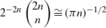 ${2^{ - 2n}}\left( {\begin{array}{*{20}{c}} {2n} \\ n\end{array}} \right) \cong {(\pi n)^{ - 1/2}}$
, and n will be of order
${2^{ - 2n}}\left( {\begin{array}{*{20}{c}} {2n} \\ n\end{array}} \right) \cong {(\pi n)^{ - 1/2}}$
, and n will be of order
 $\sqrt b $
, which hints at why
$\sqrt b $
, which hints at why
 ${b^{ - 1/4}}$
shows up in the answer. The first stage results in
${b^{ - 1/4}}$
shows up in the answer. The first stage results in
 $O({b^{ - 1/4}})$
upper and lower bounds on the stop rule; this is Lemma 4.4, which in fact was our original goal. But it is not able to get the exact coefficient of
$O({b^{ - 1/4}})$
upper and lower bounds on the stop rule; this is Lemma 4.4, which in fact was our original goal. But it is not able to get the exact coefficient of
 ${b^{ - 1/4}}$
.
${b^{ - 1/4}}$
.
Stage two, in Section 5, feeds the result of stage one back into the Value approximations developed in stage one, to obtain a much sharper approximation for V near the boundary. It is perhaps the most conceptually tricky part of the proof, with a repeated feedback argument that will be better motivated when we get there. It shows that V is essentially piecewise linear near the boundary, below and tangent at integer points of
 $\delta $
, to the quadratic approximation to
$\delta $
, to the quadratic approximation to
 ${V_W}$
near the boundary. This is Theorem 5.1, perhaps of independent interest in showing the manner in which the Brownian Value overestimates V.
${V_W}$
near the boundary. This is Theorem 5.1, perhaps of independent interest in showing the manner in which the Brownian Value overestimates V.
Finally, stage three, in Section 6, uses this improved estimate of V to go a bit further down the tree, by estimating the leaf values
 $V(u + 1,b + 2m + 1)$
for a range of m such that V is no longer just the ratio. By going just far enough down the tree, we are able to get the upper and lower bounds to come together, within an
$V(u + 1,b + 2m + 1)$
for a range of m such that V is no longer just the ratio. By going just far enough down the tree, we are able to get the upper and lower bounds to come together, within an
 $o({b^{ - 1/4}})$
error, finding the exact coefficient of
$o({b^{ - 1/4}})$
error, finding the exact coefficient of
 ${b^{ - 1/4}}$
and proving Theorem 1.1. The plan is straightforward except perhaps for Section 5, and uses standard approximations, but lots of them, so it looks worse than it is when all the approximations and sums are written out.
${b^{ - 1/4}}$
and proving Theorem 1.1. The plan is straightforward except perhaps for Section 5, and uses standard approximations, but lots of them, so it looks worse than it is when all the approximations and sums are written out.
3. Approximating the Brownian motion value
 ${V_W}$

From formula (1.1), one may differentiate under the integral sign to see that all the derivatives with respect to u are positive for
 $u \le \alpha \sqrt b $
, so they all take their maximum value on the boundary; we use that several times below. To compute derivatives, and also for numerical work, it is best to write it in terms of standard functions. We have
$u \le \alpha \sqrt b $
, so they all take their maximum value on the boundary; we use that several times below. To compute derivatives, and also for numerical work, it is best to write it in terms of standard functions. We have
 \begin{align*}{V_W}(u,b) &= (1 - {\alpha ^2})\int_0^\infty {\exp \left( {\lambda u - \frac{{{\lambda ^2}b}}{2}} \right)d\lambda }\\&=(1 - {\alpha ^2}){b^{ - 1/2}}\exp \left( {\frac{{{u^2}}}{{2b}}} \right)\int_{ - \infty }^{u/\sqrt b } {\exp \left( { - \frac{{{w^2}}}{2}} \right)dw}\\ &= (1 - {\alpha ^2}){b^{ - 1/2}}G( {u/\sqrt b })/g( {u/\sqrt b })\\ &= (1 - {\alpha ^2}){b^{ - 1/2}}H( {u/\sqrt b }),\end{align*}
where G and g are the cumulative distribution function (CDF) and probability density function (PDF) of the standard normal distribution, respectively, and we have defined
 $H(x) \,:\!= G\left( x \right)/g\left( x \right)$
. This is related to the Mills ratio by
$H(x) \,:\!= G\left( x \right)/g\left( x \right)$
. This is related to the Mills ratio by
 $H(x)=1/g(x) - m(x),$
but we do not use that. On the boundary,
$H(x)=1/g(x) - m(x),$
but we do not use that. On the boundary,
 ${u_0} = \alpha \sqrt b $
,
${u_0} = \alpha \sqrt b $
,
 ${V_W}({u_0},b) = {u_0}/b = \alpha {b^{ - 1/2}} = (1 - {\alpha ^2}){b^{ - 1/2}}H( {{u_0}/\sqrt b }) = (1 - {\alpha ^2}){b^{ - 1/2}}H\left( \alpha \right)$
, so we get the equation that alpha satisfies as
${V_W}({u_0},b) = {u_0}/b = \alpha {b^{ - 1/2}} = (1 - {\alpha ^2}){b^{ - 1/2}}H( {{u_0}/\sqrt b }) = (1 - {\alpha ^2}){b^{ - 1/2}}H\left( \alpha \right)$
, so we get the equation that alpha satisfies as
 $\alpha = (1 - {\alpha ^2})H\left( \alpha \right),$
which is useful for computing
$\alpha = (1 - {\alpha ^2})H\left( \alpha \right),$
which is useful for computing
 $\alpha $
using a library function for the Normal, or converted to an error function representation, to use that library function instead, if needed. We did that for the double-double precision numerical work for the extremely large number of positions we considered.
$\alpha $
using a library function for the Normal, or converted to an error function representation, to use that library function instead, if needed. We did that for the double-double precision numerical work for the extremely large number of positions we considered.
We will later use five derivatives of
 ${V_W}$
. Use
${V_W}$
. Use
 ${D_u}$
for derivative operator with respect to the first argument. Then
${D_u}$
for derivative operator with respect to the first argument. Then
 ${D_u}^{n}{V_W}(u,b) = (1 - {\alpha ^2}){b^{ - (n + 1)/2}}{H^{(n)}}( {u/\sqrt b } ),$
so we need to find the successive derivatives of H. It satisfies
${D_u}^{n}{V_W}(u,b) = (1 - {\alpha ^2}){b^{ - (n + 1)/2}}{H^{(n)}}( {u/\sqrt b } ),$
so we need to find the successive derivatives of H. It satisfies
 $H'(x) = xH(x) + 1$
, which makes this straightforward, and can easily be made systematic in terms of polynomials in x, similar to Hermite polynomials. One shows
$H'(x) = xH(x) + 1$
, which makes this straightforward, and can easily be made systematic in terms of polynomials in x, similar to Hermite polynomials. One shows
 \begin{align}{H^{(n)}} = {P_n}H + {Q_n},\quad \text{with } {P_{n + 1}} = P'_n + x{P_n}, {Q_{n + 1}} = {Q_n}' + {P_n}, {P_0} = 1, {Q_0} = 0.\end{align}
So
 ${D_u}^{n}{V_W}(u,b) = (1 - {\alpha ^2}){b^{ - (n + 1)/2}}\left( {P_n}( {u/\sqrt b} )H( {u/\sqrt b } ) + {Q_n}( {u/\sqrt b } ) \right)\!.$
Remark. Just like for the Hermites, we have
 $P'_n = n{P_{n - 1}}$
(an Appell sequence), so just like for the Hermites, there is a computationally practical recurrence, not involving derivatives:
$P'_n = n{P_{n - 1}}$
(an Appell sequence), so just like for the Hermites, there is a computationally practical recurrence, not involving derivatives:
 ${P_{n + 1}}(x) = x{P_n}(x) + n{P_{n - 1}}(x)$
, the only difference from the Hermites being the positive sign. But we do not need to pursue this for our purposes, we just want a few derivatives.
${P_{n + 1}}(x) = x{P_n}(x) + n{P_{n - 1}}(x)$
, the only difference from the Hermites being the positive sign. But we do not need to pursue this for our purposes, we just want a few derivatives.
On the boundary,
 $x = {u_0}/\sqrt b = \alpha \sqrt b /\sqrt b = \alpha $
and
$x = {u_0}/\sqrt b = \alpha \sqrt b /\sqrt b = \alpha $
and
 $H(\alpha ) = \alpha {(1 - {\alpha ^2})^{ - 1}},$
so
$H(\alpha ) = \alpha {(1 - {\alpha ^2})^{ - 1}},$
so
 \begin{align*}{D_u}^{n}{V_W}({u_0},b) &= (1 - {\alpha ^2}){b^{ - n/2 + 1}}\left( {{P_n}\left( \alpha \right)H\left( \alpha \right) + {Q_n}\left( \alpha \right)} \right)\\&= {b^{ - (n + 1)/2}}\left( {\alpha {P_n}\left( \alpha \right) + (1 - {\alpha ^2}){Q_n}\left( \alpha \right)} \right).\end{align*}
To get the polynomials, turn the recursion crank in (3.1) five times, resulting in
 \begin{align} {P_0} &= 1,{Q_0} = 0;\quad {P_1} = x,{Q_1} = 1;\quad {P_2} = 1 + {x^2},{Q_2} = x;\quad {P_3} = 3x + {x^3},{Q_3} = 2 + {x^2};\nonumber \\ {P_4} &= 3 + 6{x^2} + {x^4},\,{Q_4} = 5x + {x^3};\quad {P_5} = 15x + 10{x^3} + {x^5},\,{Q_5} = 8 + 9{x^2} + {x^4}.\end{align}
To prove Lemma 1.2, we use three derivatives of H, which from (3.1) and (3.2) are
 \begin{align}{H^{(1)}}(x) &= xH(x) + 1,\nonumber\\{H^{(2)}}(x) &= (1 + {x^2})H(x) + x; \\{H^{(3)}}(x) &= (3x + {x^3})H(x) + 2 + {x^2}.\nonumber\end{align}
The first five derivatives of
 $V_W$
on the boundary are
$V_W$
on the boundary are
 \begin{align}{D_u}{V_W}({u_0},b) &= {b^{ - 1}},\nonumber\\{D_u}^{2}{V_W}({u_0},b) &= {b^{ - 3/2}}2\alpha, \nonumber \\{D_u}^{3}{V_W}({u_0},b) &= {b^{ - 2}}\left( {2 + 2{\alpha ^2}} \right),\\{D_u}^{4}{V_W}({u_0},b) &= {b^{ - 5/2}}\left( {8\alpha + 2{\alpha ^3}} \right), \nonumber\\{D_u}^{5}{V_W}({u_0},b) &= {b^{ - 3}}\left( {8 + 16{\alpha ^2} + 2{\alpha ^4}} \right). \nonumber\end{align}
Let
 $\delta = {u_0} - u = \alpha \sqrt b - u$
. Using Taylor with just the first two derivatives,
$\delta = {u_0} - u = \alpha \sqrt b - u$
. Using Taylor with just the first two derivatives,
 \begin{align*}{V_W}(u,b) &= {V_W}({u_0},b) + (u - {u_0}){D_u}{V_W}({u_0},b) + \,{(u - {u_0})^2}{D_u}^{2}{V_W}({u_*},b)/2\\ &\le \alpha {b^{ - 1/2}} - \delta {b^{ - 1}} + {\delta ^2}{D_u}^{2}{V_W}({u_0},b)/2 = u{b^{ - 1}} + \alpha {\delta ^2}{b^{ - 3/2}}.\end{align*}
The inequality is because
 ${D_u}^{2}{V_W}(u,b)$
is an increasing function (recall all derivatives are positive), so is largest on the boundary. In summary,
${D_u}^{2}{V_W}(u,b)$
is an increasing function (recall all derivatives are positive), so is largest on the boundary. In summary,
 \begin{equation}{V_W}(u,b) \leqslant u{b^{ - 1}} + \alpha {\delta ^2}{b^{ - 3/2}}.\end{equation}
Using the third derivative with a similar monotonicity argument gives a lower bound, the one that we already used above in proving Lemma 2.1:
 \begin{align*}{V_W}(u,b) &\ge u{b^{ - 1}} + \alpha {\delta ^2}{b^{ - 3/2}} - (1 + {\alpha ^2}){\delta ^3}{b^{ - 2}}/3 = u{b^{ - 1}} + \alpha \sqrt{b}{\delta ^2}{b^{ - 2}} - (1 + {\alpha ^2}){\delta ^3}{b^{ - 2}}/3\\ &= u{b^{ - 1}} + (u + \delta ){\delta ^2}{b^{ - 2}} - (1 + {\alpha ^2}){\delta ^3}{b^{ - 2}}/3 \quad\text{(recall }u+ \delta = \alpha \sqrt{b} \text{)} \\ &= u{b^{ - 1}}\left( {1 + {\delta ^2}{b^{ - 1}}} \right) + {\delta ^3}{b^{ - 2}}\left( {1 - (1 + {\alpha ^2})/3} \right) \ge u{b^{ - 1}}\left( {1 + {\delta ^2}{b^{ - 1}}} \right).\end{align*}
Thus
 \begin{equation}{V_W}(u,b) \geqslant u{b^{ - 1}}\left( {1 + {\delta ^2}{b^{ - 1}}} \right).\end{equation}
Using four derivatives, the monotonicity argument yields the upper bound
 \begin{equation}{V_W}(u,b) \leqslant u{b^{ - 1}} + \alpha {\delta ^2}{b^{ - 3/2}} - (1 + {\alpha ^2}){\delta ^3}{b^{ - 2}}/3 + (4\alpha + {\alpha ^3}){\delta ^4}{b^{ - 5/2}}/12.\end{equation}
With the fifth derivative term, one gets the lower bound
 \begin{eqnarray}{V_W}(u,b) \geqslant u{b^{ - 1}} + \alpha {\delta ^2}{b^{ - 3/2}} - (1 + {\alpha ^2}){\delta ^3}{b^{ - 2}}/3 + (4\alpha + {\alpha ^3}){\delta ^4}{b^{ - 5/2}}/12\\ - (4 + 8{\alpha ^2} + {\alpha ^4}){\delta ^5}{b^{ - 3}}/60.\nonumber\end{eqnarray}
These last two inequalities are used in proving Lemma 4.2.
4. Computing bounds on tree sums
This section is based on a lot of computation. We have resorted to big-O notation rather than getting specific constants, for which we apologized earlier. We will use big-O notation in inequalities, since we deal with approximate upper and lower bounds. The meaning will probably be clear from the context, but to be certain, we define our notation. Let f,g be real-valued functions of real variable b, with
 $g(b) > 0$
for all sufficiently large b. Define
$g(b) > 0$
for all sufficiently large b. Define
 $f(b) \le O(g(b))$
to mean there exist
$f(b) \le O(g(b))$
to mean there exist
 $b_0$
and
$b_0$
and
 $K > 0$
such that
$K > 0$
such that
 $f(b) \le Kg(b), b \ge b_0$
. Usually only
$f(b) \le Kg(b), b \ge b_0$
. Usually only
 $f(b) = O(g(b))$
is defined in texts, requiring
$f(b) = O(g(b))$
is defined in texts, requiring
 $\left| f(b) \right| \le Kg(b), b \ge b_0$
. That would not be convenient for our purposes. We will write expressions such as
$\left| f(b) \right| \le Kg(b), b \ge b_0$
. That would not be convenient for our purposes. We will write expressions such as
 $f(b) \le U(b) + O\left( b^{ - 2} \right)$
, to mean there exist
$f(b) \le U(b) + O\left( b^{ - 2} \right)$
, to mean there exist
 $b_0$
and
$b_0$
and
 $K > 0$
such that
$K > 0$
such that
 $f(b) \le U(b) + K{b^{ - 2}}$
for all
$f(b) \le U(b) + K{b^{ - 2}}$
for all
 $b \ge b_0$
. That is the same as
$b \ge b_0$
. That is the same as
 $f(b) - U(b) \le O\left( {b^{ - 2}} \right)$
in our definition. U is an approximate upper bound for f, but f(b) could be arbitrarily far below U(b). This seems very natural for dealing with inequalities rather than equalities, but does not seem to be a standard notation. Similarly, still assuming
$f(b) - U(b) \le O\left( {b^{ - 2}} \right)$
in our definition. U is an approximate upper bound for f, but f(b) could be arbitrarily far below U(b). This seems very natural for dealing with inequalities rather than equalities, but does not seem to be a standard notation. Similarly, still assuming
 $g(b) > 0$
for all sufficiently large b, define
$g(b) > 0$
for all sufficiently large b, define
 $f(b) \ge O\left( g(b) \right)$
to mean there exist
$f(b) \ge O\left( g(b) \right)$
to mean there exist
 $b_0$
and
$b_0$
and
 $K>0$
such that
$K>0$
such that
 $f(b) \ge -Kg(b), b \ge b_0$
. For example,
$f(b) \ge -Kg(b), b \ge b_0$
. For example,
 $f(b) \ge U(b) + O\left({b^{-2}} \right)$
means there exist
$f(b) \ge U(b) + O\left({b^{-2}} \right)$
means there exist
 $b_0$
and
$b_0$
and
 $K>0$
such that
$K>0$
such that
 $f(b) \ge U(b) -K{b^{-2}}$
for all
$f(b) \ge U(b) -K{b^{-2}}$
for all
 $b\ge b_0$
.
$b\ge b_0$
.
Here is a way to describe the situation using set language:
 \begin{align*}O(g(b)) = \left\{ h\,:\text{ there exist }K > 0 \text{ and } b_0 \text{ such that }\left| h(b) \right| \le Kg(b)\text{ for all }b\ge b_0 \right\}.\end{align*}
Note
 $h\in O(g(b))$
implies
$h\in O(g(b))$
implies
 $|h|$
,
$|h|$
,
 $-|h|$
, and
$-|h|$
, and
 $-h$
are in O(g(b)), and
$-h$
are in O(g(b)), and
 $O(g(b))=-O(g(b))$
. Now
$O(g(b))=-O(g(b))$
. Now
 $f(b) \le O( g(b))$
means there exists
$f(b) \le O( g(b))$
means there exists
 $h \in O( g(b))$
such that
$h \in O( g(b))$
such that
 $f(b) \le h(b) \text{ for all } b$
;
$f(b) \le h(b) \text{ for all } b$
;
 $f(b) = O( g(b))$
means there exists
$f(b) = O( g(b))$
means there exists
 $h \in O(g(b))$
such that
$h \in O(g(b))$
such that
 $f(b) = h(b) \text{ for all }b$
; and
$f(b) = h(b) \text{ for all }b$
; and
 $f(b) \ge O( g(b))$
means there exists
$f(b) \ge O( g(b))$
means there exists
 $h\in O( g(b))$
such that
$h\in O( g(b))$
such that
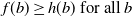 $f(b) \ge h(b)\text{ for all } b$
. That unifies the settings: for some
$f(b) \ge h(b)\text{ for all } b$
. That unifies the settings: for some
 $h \in O(g(b))$
, the inequality or equality is true when h(b) replaces O(g(b)).
$h \in O(g(b))$
, the inequality or equality is true when h(b) replaces O(g(b)).
Throughout this section, for integer
 $b>1600$
and real number u, let
$b>1600$
and real number u, let
 $\delta = \alpha \sqrt b - u$
. If
$\delta = \alpha \sqrt b - u$
. If
 $\delta < 0.38 $
or
$\delta < 0.38 $
or
 $\delta > 0.58$
, we already know whether to stop or keep going, by Lemma 2.1. But we will also want to estimate tree sums for a somewhat larger delta, to estimate leaf sums in proving Theorem 5.1. For this section, we assert that
$\delta > 0.58$
, we already know whether to stop or keep going, by Lemma 2.1. But we will also want to estimate tree sums for a somewhat larger delta, to estimate leaf sums in proving Theorem 5.1. For this section, we assert that
 $\delta \le b^p$
, where
$\delta \le b^p$
, where
 $0 \le p \le 1/10$
. We also assert that
$0 \le p \le 1/10$
. We also assert that
 $n = O(b^{1/2 + p})$
, where, as above, n indexes how far we go down the tree, looking at only the odd rows (the ones with leaves). We prove Lemma 4.3 with this generality. In our first application of Lemma 4.3, to get preliminary stop bounds, p will be 0. But in Section 5 we will use Lemma 4.3 with larger delta to get an improved estimate of Value, and then in Section 6 with larger n to finally prove Theorem 1.1.
$n = O(b^{1/2 + p})$
, where, as above, n indexes how far we go down the tree, looking at only the odd rows (the ones with leaves). We prove Lemma 4.3 with this generality. In our first application of Lemma 4.3, to get preliminary stop bounds, p will be 0. But in Section 5 we will use Lemma 4.3 with larger delta to get an improved estimate of Value, and then in Section 6 with larger n to finally prove Theorem 1.1.
Let
 ${G_n} \,:\!= {2^{ - 2n}}\left( {\begin{array}{*{20}{c}}{2n}\\n\end{array}} \right)$
, for which it is well known as a central binomial coefficient that
${G_n} \,:\!= {2^{ - 2n}}\left( {\begin{array}{*{20}{c}}{2n}\\n\end{array}} \right)$
, for which it is well known as a central binomial coefficient that
 ${G_n} \cong {\left( {\pi n} \right)^{ - 1/2}}$
; to be more precise,
${G_n} \cong {\left( {\pi n} \right)^{ - 1/2}}$
; to be more precise,
 ${\left( {\pi (n + 1/2)} \right)^{ - 1/2}} \le {G_n} \le {\left( {\pi n} \right)^{ - 1/2}}$
. The formulas that will be needed for the moments of Catalan numbers and Shapiro Catalan triangle rows can be simply expressed in terms of
${\left( {\pi (n + 1/2)} \right)^{ - 1/2}} \le {G_n} \le {\left( {\pi n} \right)^{ - 1/2}}$
. The formulas that will be needed for the moments of Catalan numbers and Shapiro Catalan triangle rows can be simply expressed in terms of
 ${G_n}$
.
${G_n}$
.
Lemma 4.1. (Catalan and Shapiro Catalan triangle moments.) We have
 \begin{align}&\sum\limits_{j = 0}^{n - 1} {{C_j}} {2^{ - 2j - 1}} = 1 - {G_n},\quad\sum\limits_{j = 0}^{n - 1} {{C_j}} {2^{ - 2j - 1}}j = n{G_n} + {G_n} - 1, \\&\sum\limits_{j = 0}^{n - 1} {{C_j}} {2^{ - 2j - 1}}{j^2} = \frac{1}{3}{n^2}{G_n} - \frac{4}{3}n{G_n} - {G_n} + 1; \nonumber\end{align}
and
 \begin{align}&{2^{ - 2n + 1}}\sum\limits_{j = 1}^n {B(n,j)} = {G_n},\quad{2^{ - 2n + 1}}\sum\limits_{j = 1}^n {jB(n,j)} = \frac{1}{2},\\&\,\,{2^{ - 2n + 1}}\sum\limits_{j = 1}^n {{j^2}B(n,j)} = n{G_n},\quad {2^{ - 2n + 1}}\sum\limits_{j = 1}^n {{j^3}B(n,j)} = \frac{{3n - 1}}{4}, \nonumber\\&{2^{ - 2n + 1}}\sum\limits_{j = 1}^n {{j^4}B(n,j)} = n(2n - 1){G_n},\quad{2^{ - 2n + 1}}\sum\limits_{j = 1}^n {{j^5}B(n,j)} = \frac{{15n(n - 1) + 2}}{8}. \nonumber\end{align}
Proof. The first statement in (4.1) is proved quickly by induction. The other two are easily proved by telescoping; we omit the details. All of (4.2) can be found in Miana and Romero [Reference Leung Lai, Yao and Aitsahlia9, pp. 5–6].
When proving Lemma 4.4, we will be using the ratio for the value, on all the leaves, to compute the leaf sum. For getting an upper bound we will be restricting n to be small enough so that the ratio is in fact the correct value on all leaves, and for the lower bound we will be restricting n to be small enough so that the ratio (which is always a lower bound) will not be far off from the correct value. But in finally proving Theorem 1.1 in Section 6, n will be large enough so that the values at some of the leaves will be significantly larger than the ratio, and we have to take that into account. It will be convenient to split the leaf sum into two parts. For general u and b, define
 ${V_E}(u,b) = V(u,b) - u/b$
, the amount the value exceeds the ratio. Let
${V_E}(u,b) = V(u,b) - u/b$
, the amount the value exceeds the ratio. Let
 \begin{align*}{S_{LR}}(n,u,b) \,:\!= \sum\limits_{m = 0}^{n - 1} {{2^{ - 2m - 1}}{C_m}} \frac{{u + 1}}{{b + 2m + 1}},\end{align*}
the contribution from the ratio, and
 \begin{align*}{S_{LE}}(n,u,b) \,:\!= \sum\limits_{m = 0}^{n - 1} {{2^{ - 2m - 1}}{C_m}} {V_E}(u + 1,b + 2m + 1),\end{align*}
from the excess over the ratio. So
 \begin{align*}{S_L} = {S_{LR}} + {S_{LE}}.\end{align*}
We have
 \begin{align*}{S_{LR}} &= \sum\limits_{m = 0}^{n - 1} {{2^{ - 2m - 1}}{C_m}} \frac{{u + 1}}{{b + 2m + 1}} = \frac{{u + 1}}{b}\sum\limits_{m = 0}^{n - 1} {{2^{ - 2m - 1}}{C_m}} {\left( {1 + \frac{{2m + 1}}{b}} \right)^{ - 1}}\\ &= \frac{{u + 1}}{b}\sum\limits_{m = 0}^{n - 1} {{2^{ - 2m - 1}}{C_m}} \left( {1 - \frac{{2m + 1}}{b} + \gamma (m)\frac{{{{\left( {2m + 1} \right)}^2}}}{{{b^2}}}} \right),\end{align*}
where
 $1 - \frac{{2m + 1}}{b} \le \gamma (m) \le 1$
. From (4.1),
$1 - \frac{{2m + 1}}{b} \le \gamma (m) \le 1$
. From (4.1),
 \begin{align*}\sum\limits_{m = 0}^{n - 1} {{2^{ - 2m - 1}}{C_m}} {\left( {2m + 1} \right)^2} &= \frac{4}{3}{n^2}{G_n} - \frac{4}{3}n{G_n} - {G_n} + 1, \\\sum\limits_{m = 0}^{n - 1} {{2^{ - 2m - 1}}{C_m}} {\left( {2m + 1} \right)} &= 2n{G_n} - 1 + {G_n},\\\sum\limits_{m = 0}^{n - 1} {{2^{ - 2m - 1}}{C_m}} &= 1 - {G_n}.\end{align*}
Since
 $\gamma (m) \le 1,$
 \begin{align*}{S_{LR}} &\le \dfrac{{u + 1}}{b}(1 - {G_n}) - \dfrac{{u + 1}}{{{b^2}}}\left( {2n{G_n} - 1 + {G_n} - \dfrac{4}{3}\dfrac{{{n^2}}}{b}{G_n} + \dfrac{4}{3}\dfrac{n}{b}{G_n} - \dfrac{1}{b} + \dfrac{{{G_n}}}{b}} \right)\\&= \dfrac{{u + 1}}{b}(1 - {G_n}) - \dfrac{{u + 1}}{{{b^2}}}\left( {2n{G_n} - 1 + {G_n} - \dfrac{4}{3}\dfrac{{{n^2}}}{b}{G_n} + O({b^{ - 1/2}})} \right),\end{align*}
where we used
 $ n = O({b^{1/2 + p}}), \frac{n}{b}{G_n} = O({b^{ - 3/4 + p/2}}) = O({b^{ - 1/2}})$
for our range of p.
$ n = O({b^{1/2 + p}}), \frac{n}{b}{G_n} = O({b^{ - 3/4 + p/2}}) = O({b^{ - 1/2}})$
for our range of p.
For a lower bound, use
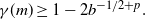 $\gamma (m) \ge 1 -2{b^{ - 1/2 + p}}.$
Note
$\gamma (m) \ge 1 -2{b^{ - 1/2 + p}}.$
Note
 ${b^{ - 1/2 + p}}({n^2}{G_n}/{b}) = O({b^{ - 3/4 + 5p/2}}) = O({b^{ - 1/2}})$
, from which it follows that the above upper bound for
${b^{ - 1/2 + p}}({n^2}{G_n}/{b}) = O({b^{ - 3/4 + 5p/2}}) = O({b^{ - 1/2}})$
, from which it follows that the above upper bound for
 $S_{LR}$
is also a lower bound, to that order.
$S_{LR}$
is also a lower bound, to that order.
Anticipating combining
 $S_{LR}$
with the row sum
$S_{LR}$
with the row sum
 $S_R$
and then getting the difference between the total and the ratio in terms of
$S_R$
and then getting the difference between the total and the ratio in terms of
 $\delta$
, write
$\delta$
, write
 \begin{align*}{S_{LR}} = \dfrac{u}{b} + \dfrac{1- (u + 1)G_n}{b} - \dfrac{\alpha}{b^{3/2}}\left(1+\dfrac{1 - \delta}{\alpha \sqrt{b}}\right)\left( {2n{G_n} - 1 + {G_n} - \dfrac{4}{3}\dfrac{{{n^2}}}{b}{G_n} + O({b^{ - 1/2}})} \right).\end{align*}
Using
 $\delta = O(b^p), n=O(p^{1/2+p})$
and
$\delta = O(b^p), n=O(p^{1/2+p})$
and
 $p \le 1/10$
, one can show
$p \le 1/10$
, one can show
 $\dfrac{\delta{n^2}{G_n}}{b^{3/2}} = O(b^{-1/2}).$
It follows that
$\dfrac{\delta{n^2}{G_n}}{b^{3/2}} = O(b^{-1/2}).$
It follows that
 \begin{align}{S_{LR}} = &\frac{u}{b} + \frac{1- (u + 1)G_n}{b}\nonumber \\& - \frac{\alpha}{b^{3/2}}\left( {2n{G_n} - 1 + {G_n} - \frac{4}{3}\frac{{{n^2}}}{b}{G_n}}+ \frac{2n{G_n}}{\alpha \sqrt{b}} - \delta \frac{2n{G_n}}{\alpha \sqrt{b}} + O({b^{ -1/2 + p}})\right).\end{align}
That takes care of the leaves; the row sum will be added to this. To get the row sum, we first replace V with
 $V_W$
and define
$V_W$
and define
 \begin{align*}{S_{RW}}(n,u,b) \,:\!= {2^{ - 2n + 1}}\sum\limits_{j = 1}^n {B(n,j)V_W(u - 2j + 1,b + 2n - 1)},\end{align*}
and use the Taylor approximation from Section 3 to compute it. This will be an upper bound for
 $S_R$
.
$S_R$
.
Lemma 4.2. (Row sum with
 $V_W$
) We have
$V_W$
) We have
 \begin{align*}{S_{RW}}(n,u,b) = \dfrac{(u + 1)G_n -1} {b} + \dfrac{\alpha }{{b^{3/2}}}X,\end{align*}
where
 \begin{align*}X\,:\!=2n{G_n}-2+2{G_n}+ 2(\alpha + 1/\alpha) \dfrac{{n{G_n}}}{{\sqrt b }} - \dfrac{(4+\alpha ^2)}{3}\dfrac{{{n^2}{G_n}}}{b}\\ + 2\delta \left( {1 - {G_n} -( \alpha + 1/\alpha) \dfrac{{n{G_n}}}{{\sqrt b }}} \right) + {\delta ^2}{G_n} + O({b^{ - 1/2 + 2p}}).\end{align*}
The proof is along the lines of the above calculation of
 $S_{LR}$
except using (4.2) instead of (4.1). But it is very much longer, so we defer the proof to Appendix B.
$S_{LR}$
except using (4.2) instead of (4.1). But it is very much longer, so we defer the proof to Appendix B.
To get a lower bound for
 $S_R$
, using Lemma 1.2 we can multiply
$S_R$
, using Lemma 1.2 we can multiply
 ${S_{RW}}$
by
${S_{RW}}$
by
 \begin{align*}1 - \dfrac{{5/12}}{{b + 2n - 1}}\left( {1 + \dfrac{1}{{\sqrt {b + 2n - 1} }}} \right) = 1 - \dfrac{5}{{12b}} + O\left( {{b^{ - 3/2 + p}}} \right).\end{align*}
Now
 \begin{align*}\dfrac{5}{{12b}}S_{RW} =\dfrac{5}{{12b}}\dfrac{uG_{n}+1}{b} + O(b^{-2})=\dfrac{\alpha }{{b^{3/2}}}\dfrac{5G_{n}}{12} + O(b^{-2+p}),\end{align*}
so
 \begin{align*}S_{RW} - \dfrac{\alpha }{{b^{3/2}}}\dfrac{5G_{n}}{12} + O(b^{-2+p}) \le S_R.\end{align*}
We get some simplification when we add
 \begin{align*}S_{LR} + S_{RW} = \dfrac{u}{b} + \dfrac{\alpha }{{b^{3/2}}}Y,\end{align*}
where
 \begin{align*}Y\,:\!=-1+{G_n}+ 2\alpha \dfrac{{n{G_n}}}{{\sqrt b }} - \dfrac{{{\alpha ^2}}}{3}\dfrac{{{n^2}{G_n}}}{b} + 2\delta \left( {1 - {G_n} - \alpha \dfrac{{n{G_n}}}{{\sqrt b }}} \right) + {\delta ^2}{G_n} + O({b^{ - 1/2 + 2p}}).\end{align*}
Thus
 \begin{align*}\dfrac{\alpha }{{b^{3/2}}}Y' \le S_{LR} + S_{R}- \dfrac{u}{b} \le \dfrac{\alpha }{{b^{3/2}}}Y,\end{align*}
where
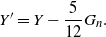 $Y'=Y-\dfrac{5}{12}G_n.$
We have proved the following result.
$Y'=Y-\dfrac{5}{12}G_n.$
We have proved the following result.
Lemma 4.3. (Bounds on tree sum.) Let
 $0 \le p \le 1/10$
,
$0 \le p \le 1/10$
,
 $n = O({b^{1/2 + p}})$
and
$n = O({b^{1/2 + p}})$
and
 $\delta \le {b^p}$
, where
$\delta \le {b^p}$
, where
 $\delta = \alpha \sqrt b - u$
. Then
$\delta = \alpha \sqrt b - u$
. Then
 \begin{align*}\frac{\alpha }{b^{3/2}}\left( C' + \delta B + {\delta ^2}A \right) \le TreeSum(n,u,b) - S_{LE} - \frac{u}{b} \le \frac{\alpha }{b^{3/2}}\left( C + \delta B + {\delta ^2}A \right),\end{align*}
where
 \begin{align*}&C \,:\!= - (1 - {C_1}{G_n})+ O(b^{ - 1/2 + 2p}),\quad C' \,:\!= - (1 - C_1'{G_n})+ O(b^{ - 1/2 + 2p}),\quad A\,:\!=G_n,\\&B\,:\!=2(1- {B_1}{G_n}),\quad\text{with }C_1\,:\!=1+2\frac{{\alpha}n}{\sqrt b}-\frac{1}{3}\frac{\alpha^2 n^2}{b},C_1'\,:\!=C_1- 5/12, B_1\,:\!=1+\frac{\alpha n}{\sqrt b}.\end{align*}
We can use this immediately to get preliminary
 $O({b^{ - 1/4}})$
bounds on the stop rule. If we do not go too far down the tree,
$O({b^{ - 1/4}})$
bounds on the stop rule. If we do not go too far down the tree,
 ${S_{LE}}$
will be zero. By Lemma 2.1, the value
${S_{LE}}$
will be zero. By Lemma 2.1, the value
 $V(u + 1,b + 2n - 1)$
at the leaf will be just the ratio if
$V(u + 1,b + 2n - 1)$
at the leaf will be just the ratio if
 $\alpha \sqrt {b + 2n - 1} - (u + 1) < 0.38$
. But
$\alpha \sqrt {b + 2n - 1} - (u + 1) < 0.38$
. But
 $\alpha \sqrt {b + 2n - 1} - (u + 1) = \alpha \sqrt b {\left( {1 + \frac{{2n - 1}}{b}} \right)^{1/2}} - (\alpha \sqrt b - \delta + 1) < \alpha n/\sqrt{b} + \delta - 1 \le 0.38$
if
$\alpha \sqrt {b + 2n - 1} - (u + 1) = \alpha \sqrt b {\left( {1 + \frac{{2n - 1}}{b}} \right)^{1/2}} - (\alpha \sqrt b - \delta + 1) < \alpha n/\sqrt{b} + \delta - 1 \le 0.38$
if
 $\alpha n / {\sqrt b} \le 0.8$
and
$\alpha n / {\sqrt b} \le 0.8$
and
 $\delta \le 0.58$
, and then
$\delta \le 0.58$
, and then
 ${S_{LE}} = 0$
. We make note of this for use later:
${S_{LE}} = 0$
. We make note of this for use later:
 \begin{equation}\alpha n/\sqrt b \le 0.8 \text{ and } \delta \le 0.58 \text{ implies } S_{LE} = 0.\end{equation}
If
 ${S_{LE}} = 0$
and
${S_{LE}} = 0$
and
 $C + \delta B + {{\delta ^2}}A \le 0$
, the tree sum will not exceed the ratio, and if
$C + \delta B + {{\delta ^2}}A \le 0$
, the tree sum will not exceed the ratio, and if
 $C' + \delta B + {{\delta ^2}}A \ge 0$
, the ratio will not exceed the tree sum. Let
$C' + \delta B + {{\delta ^2}}A \ge 0$
, the ratio will not exceed the tree sum. Let
 ${\delta _0}$
and
${\delta _0}$
and
 $\delta _0'$
be the positive numbers satisfying
$\delta _0'$
be the positive numbers satisfying
 $C + {\delta _0}B + {\delta _0^2}A = 0$
and
$C + {\delta _0}B + {\delta _0^2}A = 0$
and
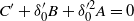 $C' + \delta _0'B + {\delta _0'^2}A = 0$
, respectively. From Lemma 2.2, it follows that
$C' + \delta _0'B + {\delta _0'^2}A = 0$
, respectively. From Lemma 2.2, it follows that
 $\alpha \sqrt b \,\, - \delta _0' \le {\beta _b} \le \alpha \sqrt b \,\, - {\delta _0}\,$
. In (a) of the next lemma, we will estimate
$\alpha \sqrt b \,\, - \delta _0' \le {\beta _b} \le \alpha \sqrt b \,\, - {\delta _0}\,$
. In (a) of the next lemma, we will estimate
 ${\delta _0}$
and
${\delta _0}$
and
 $\delta _0'$
using some convenient ns to get preliminary stop bounds from this. In addition, in (b) below we will estimate
$\delta _0'$
using some convenient ns to get preliminary stop bounds from this. In addition, in (b) below we will estimate
 ${\delta _0}$
and
${\delta _0}$
and
 $\delta _0'$
for a value of n that will be used throughout Section 5 for convenience.
$\delta _0'$
for a value of n that will be used throughout Section 5 for convenience.
Lemma 4.4. (Preliminary bounds on stop rule)
 \begin{align*}\text{(a) } \alpha \sqrt b -1/2+\frac{0.231}{\sqrt \pi}b^{-1/4}+O(b^{-1/2}) \le \beta _b \le \alpha \sqrt b -1/2+\frac{0.429}{\sqrt \pi}b^{-1/4}+O(b^{-1/2}).&&\end{align*}
(b) Let
 $n=\lfloor{ \sqrt b /2}\rfloor$
, and let
$n=\lfloor{ \sqrt b /2}\rfloor$
, and let
 $\delta _0$
and
$\delta _0$
and
 $\delta _0'$
be the positive numbers satisfying
$\delta _0'$
be the positive numbers satisfying
 $C + {\delta _0}B + {\delta _0^2}A = 0$
and
$C + {\delta _0}B + {\delta _0^2}A = 0$
and
 $C' + \delta _0'B + {\delta _0'^2}A = 0$
, respectively, where A, B, C, and C’ are as in Lemma 5.2. Then there exists
$C' + \delta _0'B + {\delta _0'^2}A = 0$
, respectively, where A, B, C, and C’ are as in Lemma 5.2. Then there exists
 $b_0$
such that
$b_0$
such that
 \begin{align*}1/2 - \frac{0.44}{\sqrt \pi}b^{-1/4} \le \delta_0 \le {\delta_0}' \le 1/2 - \frac{0.13}{\sqrt \pi}b^{-1/4},\quad b \ge b_0.\end{align*}
Proof. We will have
 $n=\Theta(b^{-1/2})$
in all cases here, so
$n=\Theta(b^{-1/2})$
in all cases here, so
 $A=G_n=O(n^{-1/2})=O(b^{-1/4})$
. For
$A=G_n=O(n^{-1/2})=O(b^{-1/4})$
. For
 $\delta _0$
, approximate the solution to the quadratic equation
$\delta _0$
, approximate the solution to the quadratic equation
 \begin{align*}\delta _0 &= \dfrac{-B+\sqrt {B^2 - 4AC}}{2A}\\&=\dfrac{-B+B\left(1-2ACB^{-2}-2{A^2}{C^2}{B^{-4}}+O(A^3)\right)}{2A}\\&=-\dfrac{C}{B}-\dfrac{AC^2}{{B^3}}+O(b^{-1/2})\end{align*}
since
 $A=O(b^{-1/4}).$
Now
$A=O(b^{-1/4}).$
Now
 \begin{align*}-\dfrac{C}{B}-\dfrac{AC^2}{{B^3}}&=\dfrac{1-C_1G_n+O(b^{-1/2+2p})}{2(1-B_1G_n)}-G_n\dfrac{\left(1-C_1G_n+O(b^{-1/2+2p})\right)^2}{8(1-B_1G_n)^3}\\&=\dfrac{1}{2}(1-C_1G_n)(1+B_1G_n)-\dfrac{G_n}{8}+O(b^{-1/2+2p})\\&=\dfrac{1}{2}-\dfrac{1}{2}\left(C_1-B_1+\dfrac{1}{4}\right)G_n+O(b^{-1/2+2p}).\end{align*}
This gives
 \begin{equation}\delta_0=\frac{1}{2}-\frac{1}{2}\left(\frac{\alpha n}{\sqrt b} - \frac{1}{3} \frac{{\alpha^2}{n^2}}{b}+\frac{1}{4}\right)G_n +O(b^{-1/2+2p}).\end{equation}
Changing C to C’ in the above calculation gives
 \begin{equation}\delta_0'=\frac{1}{2}-\frac{1}{2}\left(\frac{\alpha n}{\sqrt b} - \frac{1}{3} \frac{{\alpha^2}{n^2}}{b}-\frac{1}{6}\right)G_n +O(b^{-1/2+2p}).\end{equation}
To get an upper bound on the stop rule, we may assume
 $\delta \le 0.58$
by Lemma 2.1. Take
$\delta \le 0.58$
by Lemma 2.1. Take
 $n = \lfloor {0.8 \sqrt b / \alpha } \rfloor $
, so
$n = \lfloor {0.8 \sqrt b / \alpha } \rfloor $
, so
 ${\alpha n / \sqrt b} \le 0.8$
and
${\alpha n / \sqrt b} \le 0.8$
and
 ${S_{LE}} = 0$
, and
${S_{LE}} = 0$
, and
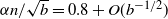 ${\alpha n / \sqrt b } = 0.8 + O({b^{ - 1/2}})$
, and
${\alpha n / \sqrt b } = 0.8 + O({b^{ - 1/2}})$
, and
 $p = 0$
. Then
$p = 0$
. Then
 \begin{align*}A = {G_n} = \dfrac{1}{{\sqrt {\pi n} }}\left( {1 + O({n^{ - 1}})} \right) = \sqrt {\dfrac{\alpha }{{0.8}}} \dfrac{{{b^{ - 1/4}}}}{{\sqrt \pi }}\left( {1 + O({b^{ - 1/2}})} \right).\end{align*}
By (4.5),
 \begin{align*}\delta _0 &= \dfrac{1}{2} - \dfrac{1}{2}\left( {0.8 - \dfrac{1}{3}0.64 + \dfrac{1}{4}} \right){G_n} + O({b^{ - 1/2}})\\ &= \dfrac{1}{2} - .4184\sqrt {\dfrac{\alpha }{{0.8}}} \dfrac{{{b^{ - 1/4}}}}{{\sqrt \pi }} + O({b^{ - 1/2}})\\ &\ge \dfrac{1}{2} - \dfrac{{0.429}}{{\sqrt \pi }}{b^{ - 1/4}} + O({b^{ - 1/2}}),\end{align*}
which proves the upper bound.
For the lower bound, we decide to take
 $n = \lfloor 1.1{\sqrt b / \alpha } \rfloor $
so
$n = \lfloor 1.1{\sqrt b / \alpha } \rfloor $
so
 $\alpha n / \sqrt b = 1.1 + O({b^{ - 1/2}})$
, to get a slightly better result. For this n, it is not quite true that
$\alpha n / \sqrt b = 1.1 + O({b^{ - 1/2}})$
, to get a slightly better result. For this n, it is not quite true that
 ${S_{LE}} = 0$
, but the expression is still a lower bound. With that choice, (4.6) gives
${S_{LE}} = 0$
, but the expression is still a lower bound. With that choice, (4.6) gives
 \begin{align*}\delta _0' &= \dfrac{1}{2} - \dfrac{1}{2}\left( {1.1 - \dfrac{1}{3}1.21 - \dfrac{1}{6}} \right)\sqrt {\dfrac{\alpha }{{1.1}}} \dfrac{{{b^{ - 1/4}}}}{{\sqrt \pi }} + O({b^{ - 1/2}})\\ &\le \dfrac{1}{2} - \dfrac{{0.231}}{{\sqrt \pi }}{b^{ - 1/4}}+ O({b^{ - 1/2}}),\end{align*}
completing the proof of (a).
For (b), we take
 $n=\lfloor \sqrt b / 2 \rfloor$
, to be used in the next section with larger
$n=\lfloor \sqrt b / 2 \rfloor$
, to be used in the next section with larger
 $\delta$
, where p is not zero. Then (4.5) and (4.6) with this n yield
$\delta$
, where p is not zero. Then (4.5) and (4.6) with this n yield
 \begin{align*}1/2 - \dfrac{{0.433}}{{\sqrt \pi }}{b^{ - 1/4}} + O({b^{ - 1/2 + 2p}}) \le {\delta _0} \le \delta _0' \le 1/2 - \dfrac{{0.137}}{{\sqrt \pi }}{b^{ - 1/4}} + O({b^{ - 1/2 + 2p}}),\end{align*}
which for some
 $b_0$
implies the result in (b).
$b_0$
implies the result in (b).
5. Improving estimate of V near the boundary, using feedback
Our next goal is to use the above to get an improved estimate of V that is very accurate when not too far from the boundary. This will allow us to go further down the backward induction tree by estimating the leaf values
 $V(u + 1,b + 2m - 1)$
for larger m, for which
$V(u + 1,b + 2m - 1)$
for larger m, for which
 $u + 1$
is more than 1/2 below the boundary and the value is no longer just the ratio. This is used in Section 6 to obtain the correct coefficient for the
$u + 1$
is more than 1/2 below the boundary and the value is no longer just the ratio. This is used in Section 6 to obtain the correct coefficient for the
 ${b^{ - 1/4}}$
term. We shall show V is approximately piecewise linear near the boundary: that is Theorem 5.1. As a first step, Lemma 4.4 showed that
${b^{ - 1/4}}$
term. We shall show V is approximately piecewise linear near the boundary: that is Theorem 5.1. As a first step, Lemma 4.4 showed that
 $V(u,b) = u/b$
if
$V(u,b) = u/b$
if
 $\delta \le 1/2\,\, - \,0.43{b^{ - 1/4}}/\sqrt \pi $
for b sufficiently large, already an improvement over our previous upper bound
$\delta \le 1/2\,\, - \,0.43{b^{ - 1/4}}/\sqrt \pi $
for b sufficiently large, already an improvement over our previous upper bound
 $V(u,b) \le u/b + \alpha {\delta ^2}{b^{ - 3/2}}$
coming from the Brownian motion case. The Brownian upper bound is too big by about
$V(u,b) \le u/b + \alpha {\delta ^2}{b^{ - 3/2}}$
coming from the Brownian motion case. The Brownian upper bound is too big by about
 $\alpha {b^{-3/2}}/4$
when delta is near 1/2.
$\alpha {b^{-3/2}}/4$
when delta is near 1/2.
We introduce a bit more notation. In this section and the next, we will be doing some estimates, in a chained fashion, an unbounded number of times, which could cause a problem if just using big-O notation. The book [Reference Graham, Knuth and Pataschnik7] gives notation (attributed to de Bruijn) which will be convenient. We let
 $f(b) = L(g(b))$
mean that
$f(b) = L(g(b))$
mean that
 $\left| {f(b)} \right| \le \left| {g(b)} \right|$
for all b. In set language,
$\left| {f(b)} \right| \le \left| {g(b)} \right|$
for all b. In set language,
 $L(g) = \left\{ {f:\left| {f(b)} \right| \le \left| {g(b)} \right|\text{ for all } b} \right\}$
. Also, let
$L(g) = \left\{ {f:\left| {f(b)} \right| \le \left| {g(b)} \right|\text{ for all } b} \right\}$
. Also, let
 ${L^ + }(g) = \left\{ {f \in L(g):f(b) \ge 0\text{ for all }b} \right\}$
. Similarly, we let
${L^ + }(g) = \left\{ {f \in L(g):f(b) \ge 0\text{ for all }b} \right\}$
. Similarly, we let
 ${O^ + }(g)$
be the non-negative members of O(g).
${O^ + }(g)$
be the non-negative members of O(g).
We assert that throughout Section 5,
 $n = \lfloor {\sqrt b /2} \rfloor $
. Lemma 4.4 (b) showed that using this n,
$n = \lfloor {\sqrt b /2} \rfloor $
. Lemma 4.4 (b) showed that using this n,
 $1/2 - 0.44{b^{ - 1/4}}/\sqrt\pi \le {\delta _0} \le \delta _0' \le 1/2 - 0.13{b^{ - 1/4}}/\sqrt\pi, b \ge {b_0}$
, where
$1/2 - 0.44{b^{ - 1/4}}/\sqrt\pi \le {\delta _0} \le \delta _0' \le 1/2 - 0.13{b^{ - 1/4}}/\sqrt\pi, b \ge {b_0}$
, where
 ${\delta _0}$
satisfies
${\delta _0}$
satisfies
 $C + {\delta _0}B + \delta _0^2A = 0$
, and
$C + {\delta _0}B + \delta _0^2A = 0$
, and
 $\delta _0'$
satisfies
$\delta _0'$
satisfies
 $C' + \delta _0'B + {\delta _0'^2}A = 0$
. A,B,C,C’ are defined in Lemma 4.3. We assert
$C' + \delta _0'B + {\delta _0'^2}A = 0$
. A,B,C,C’ are defined in Lemma 4.3. We assert
 ${b_0} > 1600$
. Now
${b_0} > 1600$
. Now
 $n \ge \sqrt b /2 - 1 = \sqrt b /2\left( {1 - 2/\sqrt b } \right)$
, so
$n \ge \sqrt b /2 - 1 = \sqrt b /2\left( {1 - 2/\sqrt b } \right)$
, so
 ${G_n} \le 1/\sqrt {\pi n} \le \sqrt {2.14/\pi } {b^{ - 1/4}} \le 0.83{b^{ - 1/4}}$
for
${G_n} \le 1/\sqrt {\pi n} \le \sqrt {2.14/\pi } {b^{ - 1/4}} \le 0.83{b^{ - 1/4}}$
for
 $b \ge {b_0}$
, a bound that will be used several times in the following. In going further away from boundary, we will use the following lemma. Recall that
$b \ge {b_0}$
, a bound that will be used several times in the following. In going further away from boundary, we will use the following lemma. Recall that
 ${V_E}(u,b) = V(u,b) - u/b$
.
${V_E}(u,b) = V(u,b) - u/b$
.
Lemma 5.1. For
 $1/2 \le \delta \le {b^p}$
, with
$1/2 \le \delta \le {b^p}$
, with
 $p \le 1/10$
,
$p \le 1/10$
,
 $n = \lfloor {\sqrt b /2} \rfloor $
, and
$n = \lfloor {\sqrt b /2} \rfloor $
, and
 $b \ge {b_0}$
,
$b \ge {b_0}$
,
 \begin{align*}{V_E}(u,b) = \frac{\alpha }{{{b^{3/2}}}}\left( {2(\delta - 1/2) + L\left( {\max \{ {\delta ^2},1\} {b^{ - 1/4}}} \right)} \right) + {S_{LE}}(n,u,b).\end{align*}
Proof. Let
 $1/2 \le \delta \le {b^p}$
. The Value is the same as the tree sum because
$1/2 \le \delta \le {b^p}$
. The Value is the same as the tree sum because
 $\delta \ge \delta _0'$
, so u is below the stop boundary.
$\delta \ge \delta _0'$
, so u is below the stop boundary.
 $\delta _0' = 1/2 - \gamma '{b^{ - 1/4}}$
for some
$\delta _0' = 1/2 - \gamma '{b^{ - 1/4}}$
for some
 $0.13/\sqrt \pi \le \gamma ' \le 0.44/\sqrt \pi $
. Let
$0.13/\sqrt \pi \le \gamma ' \le 0.44/\sqrt \pi $
. Let
 $x = \delta - \delta _0' = \delta - 1/2 + \gamma '{b^{ - 1/4}}$
. From Lemma 4.3 in the lower bound case,
$x = \delta - \delta _0' = \delta - 1/2 + \gamma '{b^{ - 1/4}}$
. From Lemma 4.3 in the lower bound case,
 \begin{align*}{V_E}(u,b) - {S_{LE}} &\ge \alpha {b^{-3/2}}\left( {C' + B\delta + A{\delta ^2}} \right)\\ &= \alpha {b^{-3/2}}\left( {C' + B\delta _0' + A{\delta _0'}^2 + Bx + A{x^2} + 2Ax\delta _0'} \right)\\ &= \alpha{b^{-3/2}}\left( {Bx + A{x^2} + 2Ax\delta _0'} \right).\end{align*}
Now
 $B = 2\left( {1 - {B_1}{G_n}} \right) = 2 - 2\left( {1 + \alpha n/\sqrt b} \right){G_n} \ge 2 - \left( {2 + \alpha } \right){G_n}$
and
$B = 2\left( {1 - {B_1}{G_n}} \right) = 2 - 2\left( {1 + \alpha n/\sqrt b} \right){G_n} \ge 2 - \left( {2 + \alpha } \right){G_n}$
and
 $A = {G_n}$
, so
$A = {G_n}$
, so
 $Bx + A{x^2} + 2Ax\delta _0'\ge 2(\delta - 1/2) + 2\gamma '{b^{ - 1/4}} +\left( { - \left( {2 + \alpha } \right)x + {x^2} + 2x\delta _0'} \right){G_n} = 2(\delta - 1/2) + 2\gamma '{b^{ - 1/4}} + x\left( {x - \alpha - 1 - 2\gamma '} \right){G_n}.$
But
$Bx + A{x^2} + 2Ax\delta _0'\ge 2(\delta - 1/2) + 2\gamma '{b^{ - 1/4}} +\left( { - \left( {2 + \alpha } \right)x + {x^2} + 2x\delta _0'} \right){G_n} = 2(\delta - 1/2) + 2\gamma '{b^{ - 1/4}} + x\left( {x - \alpha - 1 - 2\gamma '} \right){G_n}.$
But
 $x\left( {x - \alpha - 1 - 2\gamma '} \right)$
has a minimum of
$x\left( {x - \alpha - 1 - 2\gamma '} \right)$
has a minimum of
 $ - {\left( {\alpha + 1 + 2\gamma '} \right)^2}/4 > - 1$
, so
$ - {\left( {\alpha + 1 + 2\gamma '} \right)^2}/4 > - 1$
, so
 $x\left( {x - \alpha - 1 - 2\gamma '} \right){G_n} > - {b^{ - 1/4}}$
, so
$x\left( {x - \alpha - 1 - 2\gamma '} \right){G_n} > - {b^{ - 1/4}}$
, so
 ${V_E}(u,b) - {S_{LE}} \ge \alpha {b^{-3/2}}\left( {2(\delta - 1/2) - {b^{ - 1/4}}} \right)$
.
${V_E}(u,b) - {S_{LE}} \ge \alpha {b^{-3/2}}\left( {2(\delta - 1/2) - {b^{ - 1/4}}} \right)$
.
Next, let
 $x = \delta - {\delta _0} = \delta - 1/2 + \gamma {b^{ - 1/4}}$
, where
$x = \delta - {\delta _0} = \delta - 1/2 + \gamma {b^{ - 1/4}}$
, where
 $0.13/\sqrt \pi \le \gamma \le 0.44/\sqrt \pi $
. From Lemma 4.3 in the upper bound case, similar to lower bound case, we get
$0.13/\sqrt \pi \le \gamma \le 0.44/\sqrt \pi $
. From Lemma 4.3 in the upper bound case, similar to lower bound case, we get
 \begin{align*}{V_E}(u,b) - {S_{LE}} \le \alpha {b^{-3/2}}( {Bx + A{x^2} + 2Ax{\delta _0}}).\end{align*}
Now
 $B \le 2 - 2{G_n}$
, so
$B \le 2 - 2{G_n}$
, so
 \begin{align*}Bx + A{x^2} + 2Ax{\delta _0} &\le 2(\delta - 1/2) + 2\gamma {b^{ - 1/4}} - 2x{G_n} + ( {{x^2} + x}){G_n}\\ &= 2(\delta - 1/2) + 2\gamma {b^{ - 1/4}} + ({x^2} - x){G_n}. \end{align*}
If
 $\delta \le 1$
, then
$\delta \le 1$
, then
 $x \le 1$
, so
$x \le 1$
, so
 $2\gamma {b^{ - 1/4}} + ({x^2} - x){G_n} \le 2\gamma {b^{ - 1/4}} < {b^{ - 1/4}}$
. If
$2\gamma {b^{ - 1/4}} + ({x^2} - x){G_n} \le 2\gamma {b^{ - 1/4}} < {b^{ - 1/4}}$
. If
 $\delta > 1$
, then
$\delta > 1$
, then
 ${x^2} - x=(\delta - \delta_0)^2 - (\delta - \delta_0)=\delta^2 - \delta -\delta_0 (2\delta - \delta_0 -1) \le \delta^2 - 1.$
So
${x^2} - x=(\delta - \delta_0)^2 - (\delta - \delta_0)=\delta^2 - \delta -\delta_0 (2\delta - \delta_0 -1) \le \delta^2 - 1.$
So
 $2\gamma {b^{ - 1/4}} + ({x^2} - x){G_n} \le \left( {.88/\sqrt \pi } \right){b^{ - 1/4}} + ({\delta ^2} - 1)\left( {\sqrt {2.14} /\sqrt \pi } \right){b^{ - 1/4}} \le {\delta ^2}{b^{ - 1/4}}$
.
$2\gamma {b^{ - 1/4}} + ({x^2} - x){G_n} \le \left( {.88/\sqrt \pi } \right){b^{ - 1/4}} + ({\delta ^2} - 1)\left( {\sqrt {2.14} /\sqrt \pi } \right){b^{ - 1/4}} \le {\delta ^2}{b^{ - 1/4}}$
.
Now we look at
 $S_{LE},$
first considering a few small ranges of delta, to establish a pattern. If
$S_{LE},$
first considering a few small ranges of delta, to establish a pattern. If
 $0 \le \delta \le 1/2$
, then from (4.4),
$0 \le \delta \le 1/2$
, then from (4.4),
 ${S_{LE}} = 0$
. If
${S_{LE}} = 0$
. If
 $\delta \le \,{\delta _0}$
,
$\delta \le \,{\delta _0}$
,
 $V(u,b) = u/b$
. Now assume
$V(u,b) = u/b$
. Now assume
 ${\delta _0} \le \delta \le 1/2$
. Let
${\delta _0} \le \delta \le 1/2$
. Let
 $x = \delta - {\delta _0}$
, so
$x = \delta - {\delta _0}$
, so
 $x \le \gamma {b^{ - 1/4}}$
. From Lemma 4.3, proceeding as in the above proof,
$x \le \gamma {b^{ - 1/4}}$
. From Lemma 4.3, proceeding as in the above proof,
 ${V_E}(u,b) \le \alpha {b^{ - 3/2}}\left( {C + B\delta + A{\delta ^2}} \right) = \alpha {b^{ - 3/2}}\left( {Bx + A{x^2} + 2Ax{\delta _0}} \right).$
With this x, it is easy to see that
${V_E}(u,b) \le \alpha {b^{ - 3/2}}\left( {C + B\delta + A{\delta ^2}} \right) = \alpha {b^{ - 3/2}}\left( {Bx + A{x^2} + 2Ax{\delta _0}} \right).$
With this x, it is easy to see that
 $Bx + A{x^2} + 2Ax{\delta _0} \le {b^{ - 1/4}};$
we do not care to be any more precise than that. We get
$Bx + A{x^2} + 2Ax{\delta _0} \le {b^{ - 1/4}};$
we do not care to be any more precise than that. We get
 \begin{align}0 \le \delta \le 1/2 \text{ implies }{V_E}(u,b) = \frac{\alpha }{{{b^{3/2}}}}\left( {{L^ + }({b^{ - 1/4}})} \right),\quad b \ge b_0.\end{align}
When
 $1/2 \le \delta $
, the value V(u,b) is the tree sum, bigger than the ratio. The leaf sum part involves
$1/2 \le \delta $
, the value V(u,b) is the tree sum, bigger than the ratio. The leaf sum part involves
 $V(u + 1,b + 2m + 1)$
, where
$V(u + 1,b + 2m + 1)$
, where
 $m \le n - 1$
. The distance of
$m \le n - 1$
. The distance of
 $u + 1$
below the boundary is
$u + 1$
below the boundary is
 $d = \max \left\{ {\alpha \sqrt {b + 2m + 1} \,\, - (u + 1),0} \right\}$
. But
$d = \max \left\{ {\alpha \sqrt {b + 2m + 1} \,\, - (u + 1),0} \right\}$
. But
 $\alpha \sqrt {b + 2m + 1} \,\, - (u + 1) = \alpha \sqrt b {\left( {1 + (2m + 1)/b} \right)^{1/2}} - \alpha \sqrt b + \delta - 1$
. Standard estimates give
$\alpha \sqrt {b + 2m + 1} \,\, - (u + 1) = \alpha \sqrt b {\left( {1 + (2m + 1)/b} \right)^{1/2}} - \alpha \sqrt b + \delta - 1$
. Standard estimates give
 $1 + m{b^{ - 1}} \le {\left( {1 + (2m + 1)/b} \right)^{1/2}} \le 1 + m{b^{ - 1}} + {b^{ - 1}}/2$
, so
$1 + m{b^{ - 1}} \le {\left( {1 + (2m + 1)/b} \right)^{1/2}} \le 1 + m{b^{ - 1}} + {b^{ - 1}}/2$
, so
 $\alpha m{b^{ - 1/2}} \le \alpha \sqrt b {\left( {1 + (2m + 1)/b} \right)^{1/2}} - \alpha \sqrt b \le \alpha m{b^{ - 1/2}} + \alpha {b^{ - 1/2}}/2$
. Thus for
$\alpha m{b^{ - 1/2}} \le \alpha \sqrt b {\left( {1 + (2m + 1)/b} \right)^{1/2}} - \alpha \sqrt b \le \alpha m{b^{ - 1/2}} + \alpha {b^{ - 1/2}}/2$
. Thus for
 $m \le n-1$
,
$m \le n-1$
,
 \begin{align}d = \left( {\alpha \sqrt {b + 2m + 1} \,\, - (u + 1)} \right)^+ = \left( {\frac{{\alpha m}}{{\sqrt b }} + \delta - 1 + {L^ + }\left( {\alpha {b^{ - 1/2}}/2} \right)} \right)^+.\end{align}
We will use this in several places below.
Consider
 $1/2 \le \delta \le 1$
. Since
$1/2 \le \delta \le 1$
. Since
 $\delta \le 1$
,
$\delta \le 1$
,
 $d \le \alpha m/\sqrt b + {L^ + }\left( {\alpha {b^{ - 1/2}}/2} \right)$
. But
$d \le \alpha m/\sqrt b + {L^ + }\left( {\alpha {b^{ - 1/2}}/2} \right)$
. But
 $m \le \sqrt b /2$
, so
$m \le \sqrt b /2$
, so
 $d \le \alpha /2 + {L^ + }\left( {\alpha {b^{ - 1/2}}/2} \right)$
, and computation shows this is less than
$d \le \alpha /2 + {L^ + }\left( {\alpha {b^{ - 1/2}}/2} \right)$
, and computation shows this is less than
 $1/2 - 0.44{b^{ - 1/4}}/\sqrt \pi $
if
$1/2 - 0.44{b^{ - 1/4}}/\sqrt \pi $
if
 $b \ge {b_0}$
, assumed. So
$b \ge {b_0}$
, assumed. So
 ${V_E}(u + 1,b + 2m + 1) = 0$
(that is, the value is just the ratio), and
${V_E}(u + 1,b + 2m + 1) = 0$
(that is, the value is just the ratio), and
 ${S_{LE}} = 0$
. Then Lemma 5.1 gives
${S_{LE}} = 0$
. Then Lemma 5.1 gives
 \begin{align}1/2 \le \delta \le 1 \text{ implies }{V_E}(u,b) = \frac{\alpha }{{{b^{3/2}}}}\left( {2(\delta - 1/2) + L({b^{ - 1/4}})} \right), b \ge {b_0}.\end{align}
Our improved estimate so far for
 $V_E(u,b)$
,
$V_E(u,b)$
,
 $0 \le \delta \le 1$
, is piecewise linear plus an
$0 \le \delta \le 1$
, is piecewise linear plus an
 $O({b^{ - 1/4}})$
correction; zero for delta from 0 to 1/2, then slope
$O({b^{ - 1/4}})$
correction; zero for delta from 0 to 1/2, then slope
 $2 \alpha b^{-3/2}$
from 1/2 to 1. The piecewise-linear part is accurate to order
$2 \alpha b^{-3/2}$
from 1/2 to 1. The piecewise-linear part is accurate to order
 ${b^{ - 1/4}}$
, relative to
${b^{ - 1/4}}$
, relative to
 $b^{-3/2}$
. Compare this to our previous upper bound estimate from the Brownian value,
$b^{-3/2}$
. Compare this to our previous upper bound estimate from the Brownian value,
 $V_E \le {V_W}(u,b) - u{b^{ - 1}} \le \alpha {b^{ - 3/2}}{\delta ^2}$
, and about equal to that for delta small compared to
$V_E \le {V_W}(u,b) - u{b^{ - 1}} \le \alpha {b^{ - 3/2}}{\delta ^2}$
, and about equal to that for delta small compared to
 $\sqrt b $
; that is, quadratic for delta not too big. Our piecewise-linear function matches the quadratic one at
$\sqrt b $
; that is, quadratic for delta not too big. Our piecewise-linear function matches the quadratic one at
 $\delta = 0$
and
$\delta = 0$
and
 $\delta = 1$
, and is tangent to the parabola at those points. At
$\delta = 1$
, and is tangent to the parabola at those points. At
 $\delta = 1/2$
, the piecewise-linear function is below the parabola by 1/4. That is where the upper bound from the Brownian is worst.
$\delta = 1/2$
, the piecewise-linear function is below the parabola by 1/4. That is where the upper bound from the Brownian is worst.
Now we show that same linear piece continues up to 3/2. Let
 $1 \le \delta \le 3/2$
. The distance of
$1 \le \delta \le 3/2$
. The distance of
 $u + 1$
from the boundary
$u + 1$
from the boundary
 $\alpha \sqrt {b + 2m + 1}$
is, from (5.2),
$\alpha \sqrt {b + 2m + 1}$
is, from (5.2),
 $d = \alpha m{b^{ - 1/2}} + \delta - 1 + {L^ + }\left( {\alpha {b^{ - 1/2}}/2} \right) \le \alpha /2 + 1/2 + {L^ + }\left( {\alpha {b^{ - 1/2}}/2} \right) \le 1$
, for
$d = \alpha m{b^{ - 1/2}} + \delta - 1 + {L^ + }\left( {\alpha {b^{ - 1/2}}/2} \right) \le \alpha /2 + 1/2 + {L^ + }\left( {\alpha {b^{ - 1/2}}/2} \right) \le 1$
, for
 $b \ge {b_0}$
. If also
$b \ge {b_0}$
. If also
 $d \ge 1/2$
, we can feed this into (5.3) with d in the role of
$d \ge 1/2$
, we can feed this into (5.3) with d in the role of
 $\delta $
and
$\delta $
and
 $b + 2m + 1$
in the role of b. This is the key feedback idea that will be used in proving Theorem 5.1. If
$b + 2m + 1$
in the role of b. This is the key feedback idea that will be used in proving Theorem 5.1. If
 $d < 1/2$
, (5.3) still holds if we replace
$d < 1/2$
, (5.3) still holds if we replace
 $d - 1/2$
by
$d - 1/2$
by
 $(d - 1/2)^+$
. So
$(d - 1/2)^+$
. So
 ${V_E}(u + 1,b + 2m + 1) = \alpha {\left( {b + 2m + 1} \right)^{ - 3/2}}\left( 2(d - 1/2)^+ + L({b^{ - 1/4}}) \right)$
. Note
${V_E}(u + 1,b + 2m + 1) = \alpha {\left( {b + 2m + 1} \right)^{ - 3/2}}\left( 2(d - 1/2)^+ + L({b^{ - 1/4}}) \right)$
. Note
 $d - 1/2 \le \alpha m{b^{ - 1/2}} + \alpha {b^{ - 1/2}}/2$
. Using (4.1),
$d - 1/2 \le \alpha m{b^{ - 1/2}} + \alpha {b^{ - 1/2}}/2$
. Using (4.1),
 \begin{align*}{S_{LE}} &\le \sum\limits_{m = 0}^{n - 1} {{2^{ - 2m - 1}}{C_m}\alpha {{\left( {b + 2m + 1} \right)}^{ - 3/2}}\left( {2\alpha m{b^{ - 1/2}} + \alpha {b^{ - 1/2}} + {b^{ - 1/4}}} \right)}\\ &\le \alpha {b^{ - 3/2}}\left( {n{G_n}2\alpha {b^{ - 1/2}} + \alpha {b^{ - 1/2}} + {b^{ - 1/4}}} \right) \le \alpha {b^{ - 3/2}}\left( {2{b^{ - 1/4}}} \right),\quad \mbox{for }b \ge {b_0}.\end{align*}
Using Lemma 5.1 and adding in this estimate of
 $S_{LE}$
gives the same answer as (5.3), except for increasing the error bound, which then covers (5.3) as well:
$S_{LE}$
gives the same answer as (5.3), except for increasing the error bound, which then covers (5.3) as well:
 \begin{align}1/2 \le \delta \le 3/2 \text{ implies }{V_E}(u,b) = \frac{\alpha }{{{b^{3/2}}}}\left( {2(\delta - 1/2) + L(5{b^{ - 1/4}})} \right),\quad b \ge {b_0}.\end{align}
Now that we see that the piecewise-linear function below and tangent to the quadratic at integers gets us this far, we guess that this pattern continues (up to some error), and Theorem 5.1 will prove this. By stepping along one 1/2 unit at a time, and feeding the result back into the previous step the way we did to get to 3/2, we will get our piecewise-linear estimate that will be good enough for our purpose.
Theorem 5.1. (Value near the boundary.) Assume
 $b \ge {b_0}$
. Then
$b \ge {b_0}$
. Then
 \begin{align*}{V_E}&(u,b) =\frac{\alpha }{{{b^{3/2}}}}\left\{ {2j(\delta - 1/2) - j(j - 1) + L\left( {{M_j}{b^{ - 1/4}}} \right)} \right\},\quad j - 1/2 \le \delta \le j + 1/2,\\&0 \le j \le {b^{1/10}},\end{align*}
where j is integral,
 $M_0 = 1$
, and
$M_0 = 1$
, and
 $M_j \le 5{j^3}, j \ge 1$
.
$M_j \le 5{j^3}, j \ge 1$
.
Figure 7 is a graph of the piecewise-linear function
 $2j(\delta - 1/2) - j(j - 1)$
for
$2j(\delta - 1/2) - j(j - 1)$
for
 $0 \le \delta \le 2.5$
, compared to
$0 \le \delta \le 2.5$
, compared to
 ${\delta ^2}$
. which is shown dashed. The j changes at the half-integer points. It is tangent to the parabola at integers, and 1/4 below the parabola at half-integers, with a straight-line graph between half-integer points.
${\delta ^2}$
. which is shown dashed. The j changes at the half-integer points. It is tangent to the parabola at integers, and 1/4 below the parabola at half-integers, with a straight-line graph between half-integer points.

Figure 7. Graph of piecewise-linear approximation to scaled excess value,
 ${\alpha ^{-1}}{b^{3/2}}V_E$
, as a function of distance
${\alpha ^{-1}}{b^{3/2}}V_E$
, as a function of distance
 $\delta$
from boundary. The dashed curve is
$\delta$
from boundary. The dashed curve is
 $\delta ^2$
, the quadratic approximation to the scaled excess value that comes from the Brownian upper bound.
$\delta ^2$
, the quadratic approximation to the scaled excess value that comes from the Brownian upper bound.
The induction proof of this theorem uses the same feedback logic above that established the case
 $j=1$
at (5.4), but it is long and tedious, so we put it in Appendix C.
$j=1$
at (5.4), but it is long and tedious, so we put it in Appendix C.
6. Proof of Theorem 1.1
In this section, let
 ${n_0} = \lfloor {\sqrt b /\alpha } \rfloor $
, so
${n_0} = \lfloor {\sqrt b /\alpha } \rfloor $
, so
 $\alpha {n_0}/\sqrt{b} = 1 - {L^ + }(\alpha {b^{ - 1/2}})$
and
$\alpha {n_0}/\sqrt{b} = 1 - {L^ + }(\alpha {b^{ - 1/2}})$
and
 $\alpha /\sqrt{b} = 1/{n_0} - {L^ + }(\alpha {b^{ - 1}})$
; we will see that replacing
$\alpha /\sqrt{b} = 1/{n_0} - {L^ + }(\alpha {b^{ - 1}})$
; we will see that replacing
 $\sqrt b /\alpha $
by its integer part is not going to matter, to the order of interest. Let
$\sqrt b /\alpha $
by its integer part is not going to matter, to the order of interest. Let
 $0 < p \le 1/10$
, to be decided later (in the end, it will be 1/12). Let
$0 < p \le 1/10$
, to be decided later (in the end, it will be 1/12). Let
 $J + 1 = \left\lfloor {{b^p}} \right\rfloor $
, so
$J + 1 = \left\lfloor {{b^p}} \right\rfloor $
, so
 $J \sim {b^p}$
. In this section, we are going to let
$J \sim {b^p}$
. In this section, we are going to let
 $n = (J + 1){n_0}$
, so n will go to infinity faster than
$n = (J + 1){n_0}$
, so n will go to infinity faster than
 $\sqrt b $
, but only slightly. This larger n will cause some of the leaf values to be more than just the ratio. By dividing n into J stretches of size
$\sqrt b $
, but only slightly. This larger n will cause some of the leaf values to be more than just the ratio. By dividing n into J stretches of size
 ${n_0}$
, we will get a linear approximation to the extra part of the leaf values,
${n_0}$
, we will get a linear approximation to the extra part of the leaf values,
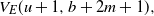 ${V_E}(u + 1,b + 2m + 1),$
on each stretch, via Theorem 5.1; that is Lemma 6.1.
${V_E}(u + 1,b + 2m + 1),$
on each stretch, via Theorem 5.1; that is Lemma 6.1.
Assume throughout this section that
 $b \ge {b_0}$
and
$b \ge {b_0}$
and
 $\delta = \alpha \sqrt b - u.$
In this section, where we seek the stop rule, we only consider
$\delta = \alpha \sqrt b - u.$
In this section, where we seek the stop rule, we only consider
 $\delta$
in the range
$\delta$
in the range
 $1/2 - \,0.44{\pi ^{ - 1/2}}{b^{ - 1/4}} \le \delta \le 1/2 - \,0.13{\pi ^{ - 1/2}}{b^{ - 1/4}}$
, because we already know that the exact stop value occurs for some delta in this range. So
$1/2 - \,0.44{\pi ^{ - 1/2}}{b^{ - 1/4}} \le \delta \le 1/2 - \,0.13{\pi ^{ - 1/2}}{b^{ - 1/4}}$
, because we already know that the exact stop value occurs for some delta in this range. So
 $\delta = 1/2 - \gamma {b^{ - 1/4}}$
, for some
$\delta = 1/2 - \gamma {b^{ - 1/4}}$
, for some
 $0.13{\pi ^{ - 1/2}} \le \gamma \le 0.44{\pi ^{ - 1/2}}$
.
$0.13{\pi ^{ - 1/2}} \le \gamma \le 0.44{\pi ^{ - 1/2}}$
.
We will estimate
 $V_E(u+1,b+2m+1)$
by using results from Section 5, when
$V_E(u+1,b+2m+1)$
by using results from Section 5, when
 $u+1$
is further away from
$u+1$
is further away from
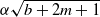 $\alpha \sqrt{b+2m+1}$
, but in this section we will use d instead of
$\alpha \sqrt{b+2m+1}$
, but in this section we will use d instead of
 $\delta$
to denote that distance, since
$\delta$
to denote that distance, since
 $\delta$
is fixed throughout this section to be
$\delta$
is fixed throughout this section to be
 $\alpha \sqrt b - u$
. To avoid confusion, note that we will be using results from Section 5 with d in the role of
$\alpha \sqrt b - u$
. To avoid confusion, note that we will be using results from Section 5 with d in the role of
 $\delta$
there, and
$\delta$
there, and
 $b+2m+1$
in the role of b.
$b+2m+1$
in the role of b.
By letting J go to infinity with b, at just the right rate, we can make the upper and lower bounds from Lemma 4.3 come together, to order
 $o({b^{ - 1/4}})$
, as we will see later.
$o({b^{ - 1/4}})$
, as we will see later.
Lemma 6.1. There exists K such that for
 $\delta = 1/2 - {L^ + }({b^{ - 1/4}})$
and for
$\delta = 1/2 - {L^ + }({b^{ - 1/4}})$
and for
 $j = 1,\ldots,J$
,
$j = 1,\ldots,J$
,
 \begin{align*}{V_E}(u + 1,b + 2m + 1) = \frac{\alpha }{{{b^{3/2}}}}\left\{ {2j\frac{m}{{{n_0}}} - j(j + 1) + L\left( {K{j^3}{b^{ - 1/4}}} \right)} \right\},\quad j{n_0} \le m \le (j + 1){n_0}.\end{align*}
Proof. Let
 $j{n_0} \le m \le (j + 1){n_0}.$
Then
$j{n_0} \le m \le (j + 1){n_0}.$
Then
 $d = \alpha \sqrt {b + 2m + 1}- (u + 1)= \alpha \sqrt b {\left( {b + 2m + 1} \right)^{1/2}} - (\alpha \sqrt b - \delta + 1).$
This can be estimated using the binomial expansion, similar to what was done to get (5.2), but now m is bounded below by
$d = \alpha \sqrt {b + 2m + 1}- (u + 1)= \alpha \sqrt b {\left( {b + 2m + 1} \right)^{1/2}} - (\alpha \sqrt b - \delta + 1).$
This can be estimated using the binomial expansion, similar to what was done to get (5.2), but now m is bounded below by
 ${n_0}$
and above by
${n_0}$
and above by
 ${b^p}{n_0}$
, so the result is different. One can show
${b^p}{n_0}$
, so the result is different. One can show
 $1 + m/b - {b^{ - 1 + 2p}}/(2{\alpha ^2}) \le {\left( {1 + (2m + 1)/b} \right)^{1/2}} \le 1 + m/b,$
so
$1 + m/b - {b^{ - 1 + 2p}}/(2{\alpha ^2}) \le {\left( {1 + (2m + 1)/b} \right)^{1/2}} \le 1 + m/b,$
so
 $d \le \alpha m/\sqrt{b} + \delta - 1 \le m/n_0 - 1/2 - \gamma {b^{ - 1/4}};$
and
$d \le \alpha m/\sqrt{b} + \delta - 1 \le m/n_0 - 1/2 - \gamma {b^{ - 1/4}};$
and
 $d \ge \alpha m/\sqrt{b} - {b^{ - 1/2 + 2p}}/(2\alpha) + \delta - 1 \ge m/n_0 - m\alpha/b - {b^{ - 1/2 + 2p}}/(2\alpha) - 1/2 - \gamma {b^{ - 1/4}} \ge m/n_0 - 1/2 - {b^{ - 1/4}}.$
Putting it all together,
$d \ge \alpha m/\sqrt{b} - {b^{ - 1/2 + 2p}}/(2\alpha) + \delta - 1 \ge m/n_0 - m\alpha/b - {b^{ - 1/2 + 2p}}/(2\alpha) - 1/2 - \gamma {b^{ - 1/4}} \ge m/n_0 - 1/2 - {b^{ - 1/4}}.$
Putting it all together,
 $d = m/n_0 - 1/2 - \psi {b^{ - 1/4}},$
for some
$d = m/n_0 - 1/2 - \psi {b^{ - 1/4}},$
for some
 $0 \le \psi \le 1,$
is good enough. Note
$0 \le \psi \le 1,$
is good enough. Note
 $j - 1/2 \le m/n_0 - 1/2 \le j + 1/2.$
-
(i) If
$j - 1/2 \le d = m/n_0 - 1/2 - \psi {b^{ - 1/4}} \le j + 1/2,$
then Theorem 5.1 gives Approximating
\begin{align*}{V_E}(u + 1,b + 2m + 1) = \alpha {(b + 2m + 1)^{ - 3/2}}\left\{ \begin{array}{l}2j\left( m/n_0 - 1/2 - \psi {b^{ - 1/4}} - 1/2 \right)\\ - j(j - 1) + L\left( {5{j^3}{b^{ - 1/4}}} \right)\end{array} \right\}.\end{align*}
$\alpha {(b + 2m + 1)^{ - 3/2}}$
and with an argument similar to earlier ones,
\begin{align*}{V_E}(u + 1,b + 2m + 1) = \alpha {b^{ - 3/2}}\left\{ {2jm/n_0 - j(j + 1) + L\left( {(5{j^3} + 2{j^2} + 2j){b^{ - 1/4}}} \right)} \right\}.\end{align*}
-
(ii) Suppose, however, that
$d = m/{n_0} - 1/2 - \psi {b^{ - 1/4}} \le j - 1/2:$
the
$\psi {b^{ - 1/4}}$
term bumped us down into the next interval below. But just barely:
$m/{n_0} - 1/2 \ge j - 1/2,$
and
$m/n_0 - 1/2 - \psi {b^{ - 1/4}} \le j - 1/2,$
so
$m/{n_0} = j + {L^ + }(\psi {b^{ - 1/4}}).$
Using Theorem 5.1, but with
$j - 1$
in place of j, Using
\begin{align*}{V_E}(u + 1,b + 2m + 1) = \alpha {(b + 2m + 1)^{ - 3/2}}\left\{ \begin{array}{l}2(j - 1)\left( {m/{n_0} - 1/2 - \psi {b^{ - 1/4}} - 1/2} \right)\\ - (j - 1)(j - 2) + L\left( {5{{(j - 1)}^3}{b^{ - 1/4}}} \right)\end{array} \right\}.\end{align*}
$m/{n_0} = j + {L^ + }(\psi {b^{ - 1/4}})$
and arguments similar to previous ones, Cases (i) and (ii) are covered by
\begin{align*}{V_E}(u + 1,b + 2m + 1) = \alpha {b^{ - 3/2}}\left\{ \begin{array}{l}2jm/{n_0} - j(j + 1)\\ + L\left( {\left( {5{{(j - 1)}^3} + 2{j^2} + 2j} \right){b^{ - 1/4}}} \right)\end{array} \right\}.\end{align*}
${V_E}(u + 1,b + 2m + 1)$
$ = \alpha {b^{ - 3/2}}\left\{ {2jm/{n_0} - j(j + 1) + L\left( {9{j^3}{b^{ - 1/4}}} \right)} \right\}$
, so
$K = 9$
is good enough.


To prove the main theorem, we have to put in the extra contribution
 ${S_{LE}}$
to the leaf sum that comes from the leaf values that exceed the ratio, when going down to
${S_{LE}}$
to the leaf sum that comes from the leaf values that exceed the ratio, when going down to
 $n=(J + 1){n_0}.$
Lemma 6.2.
 \begin{align*}{S_{LE}} = \frac{\alpha }{{{b^{3/2}}}}\left\{ {{C_{LE}}{G_n} + O\left( {{J^{5/2}}{b^{ - 1/2}}} \right)} \right\},\end{align*}
where
 \begin{align*}{C_{LE}} \,:\!= \frac{1}{3}{J^2} - \frac{1}{3}J - 4\zeta (\! -1/2)\sqrt {J + 1} + O(1).\end{align*}
Proof. Let
 ${S_{LE}}(j)$
denote the contribution to
${S_{LE}}(j)$
denote the contribution to
 ${S_{LE}}$
from summing
${S_{LE}}$
from summing
 ${{2^{ - 2m - 1}}{C_m}} {V_E}(u + 1,b + 2m + 1)$
over m in the range
${{2^{ - 2m - 1}}{C_m}} {V_E}(u + 1,b + 2m + 1)$
over m in the range
 $j{n_0} \le m < (j + 1){n_0}$
. Let
$j{n_0} \le m < (j + 1){n_0}$
. Let
 $W(j) = {S_{LE}}(j){b^{3/2}}/\alpha$
.
$W(j) = {S_{LE}}(j){b^{3/2}}/\alpha$
.
 $W(0) = 0$
. Now let
$W(0) = 0$
. Now let
 $j \ge 1$
. By Lemmas 6.1 and 4.1,
$j \ge 1$
. By Lemmas 6.1 and 4.1,
 \begin{align*}W(j) &= \frac{{2j}}{{{n_0}}}\sum\limits_{m = j{n_0}}^{(j + 1){n_0} - 1} {m{2^{ - 2m - 1}}{C_m}} - \left( {j(j + 1) + L\left( {K{j^3}{b^{ - 1/4}}} \right)} \right)\sum\limits_{m = j{n_0}}^{(j + 1){n_0} - 1} {{2^{ - 2m - 1}}{C_m}} \\&= \frac{{2j}}{{{n_0}}}\left( {(j + 1){n_0}{G_{(j + 1){n_0}}} - j{n_0}{G_{j{n_0}}}} \right) - \left( {\frac{{2j}}{{{n_0}}} + j(j + 1) + L\left( {K{j^3}{b^{ - 1/4}}} \right)} \right)\left( {{G_{j{n_0}}} - {G_{(j + 1){n_0}}}} \right)\\&= 3j(j + 1){G_{(j + 1){n_0}}} - j(3j + 1){G_{j{n_0}}} + L\left( {(K + 1){j^3}{b^{ - 1/4}}} \right)\left( {{G_{j{n_0}}} - {G_{(j + 1){n_0}}}} \right).\end{align*}
Now
 \begin{align*}{G_{j{n_0}}} - {G_{(j + 1){n_0}}} \le \dfrac{1}{{\sqrt \pi }}\left( {\dfrac{1}{{\sqrt {{n_0}j} }} - \dfrac{1}{{\sqrt {{n_0}(j + 1) + 1/2} }}} \right) \le \dfrac{{{j^{ - 3/2}}}}{{2\sqrt {\pi {n_0}} }} \le \dfrac{{{j^{ - 3/2}}{b^{ - 1/4}}}}{{2\sqrt \pi }},\end{align*}
and
 \begin{align*}\dfrac{1}{{\sqrt {k\pi } }}\left( {1 - \dfrac{1}{{4k}}} \right) \le {G_k} \le \dfrac{1}{{\sqrt {k\pi } }} \implies \dfrac{{{G_{j{n_0}}}}}{{{G_{(J + 1){n_0}}}}} = \dfrac{{\sqrt {J + 1} }}{{\sqrt j }}\left( {1 + L\left( {\dfrac{1}{{4j{n_0}}}} \right)} \right).\end{align*}
Using the latter to express
 $G_{jn_0}$
and
$G_{jn_0}$
and
 $G_{(j+1)n_0}$
in terms of
$G_{(j+1)n_0}$
in terms of
 $G_{(J+1)n_0}$
,
$G_{(J+1)n_0}$
,
 \begin{align*}W(j) &= \left( \begin{array}{l}3j\sqrt {j + 1} \left( {1 + L\left( {{{(4(j + 1){n_0})}^{ - 1}}} \right)} \right)\\ - \sqrt j (3j + 1)\left( {1 + L\left( {{{(4j{n_0})}^{ - 1}}} \right)} \right)\end{array} \right)\sqrt {J + 1} {G_{(J + 1){n_0}}} + L\left( {(K + 1){j^{3/2}}{b^{ - 1/2}}} \right)\\&= \left( {3j\sqrt {(j + 1)} - 3(j - 1)\sqrt j - 4\sqrt j } \right)\sqrt {J + 1} {G_n} + L\left( {(K + 2){j^{3/2}}{b^{ - 1/2}}} \right).\end{align*}
We wrote it that way so that telescoping occurs for the first two terms when summing
 \begin{align*}\sum\limits_{j=1}^{J}W(j)&={\left( {\sum\limits_{j = 1}^J {\left(3j\sqrt {(j + 1)} - 3(j - 1)\sqrt {j}\right)} - 4\sum\limits_{j = 1}^J {\sqrt j } } \right)\sqrt {J + 1} {G_n} + O\left( {J^{5/2}}{ b^{ - 1/2}} \right)}\\&= {\left( {3J\sqrt {(J + 1)} - 4\sum\limits_{j = 1}^J {\sqrt j } } \right)\sqrt {J + 1} {G_n} + O\left( {{J^{5/2}}{b^{ - 1/2}}} \right)}.\end{align*}
At this point we are through summing over an unbounded range, so we replaced the big-L with big-O notation, with no harm. There is a well-known asymptotic formula for the sum of square roots as a generalized harmonic number:
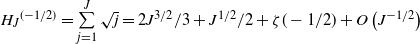 ${H_J}^{( -1/2)} = \sum\limits_{j = 1}^J {\sqrt j } = 2{J^{3/2}}/3 + {J^{1/2}}/2 + \zeta ( -1/2) + O\left( {{J^{ - 1/2}}} \right)$
[Reference Graham, Knuth and Pataschnik7, p. 594]. And
${H_J}^{( -1/2)} = \sum\limits_{j = 1}^J {\sqrt j } = 2{J^{3/2}}/3 + {J^{1/2}}/2 + \zeta ( -1/2) + O\left( {{J^{ - 1/2}}} \right)$
[Reference Graham, Knuth and Pataschnik7, p. 594]. And
 $\sqrt {J + 1} = {J^{1/2}} + {J^{ - 1/2}}/2 + O\left( {{J^{ - 3/2}}} \right)$
, so
$\sqrt {J + 1} = {J^{1/2}} + {J^{ - 1/2}}/2 + O\left( {{J^{ - 3/2}}} \right)$
, so
 $4{H_J}^{( -1/2)}\sqrt {J + 1} = 8{J^2}/3 + 10J/3 + 4\zeta ( -1/2)\sqrt {J + 1} + O(1),$
and
$4{H_J}^{( -1/2)}\sqrt {J + 1} = 8{J^2}/3 + 10J/3 + 4\zeta ( -1/2)\sqrt {J + 1} + O(1),$
and
 $3J(J + 1) - 4{H_J}^{( - 1/2)}\sqrt {J + 1} = {J^2}/3 - J/3 - 4\zeta ( -1/2)\sqrt {J + 1} + O(1).$
So
$3J(J + 1) - 4{H_J}^{( - 1/2)}\sqrt {J + 1} = {J^2}/3 - J/3 - 4\zeta ( -1/2)\sqrt {J + 1} + O(1).$
So
 ${S_{LE}} = \alpha {b^{ - 3/2}}\left\{ {\left( {{J^2}/3 - J/3 - 4\zeta ( -1/2)\sqrt {J + 1} } +O(1)\right){G_n} + O\left( {{J^{5/2}}{b^{ - 1/2}}} \right)} \right\}.$
We can now conclude the proof of Theorem 1.1.
Proof of Theorem 1.1. Go back to Lemma 4.3, to get the bounds on the tree sum using this n, adding in the
 ${S_{LE}}$
term from Lemma 6.2. Our assumption about J implies
${S_{LE}}$
term from Lemma 6.2. Our assumption about J implies
 $n = O({b^{1/2 + p}})$
with
$n = O({b^{1/2 + p}})$
with
 $p \le 1/10$
, so Lemma 4.3 applies. For the upper bound,
$p \le 1/10$
, so Lemma 4.3 applies. For the upper bound,
 $TreeSum(n,u,b) - u/b \le \alpha {b^{ - 3/2}}\left\{ {C + \delta B + {\delta ^2}A} \right\} + {S_{LE}} = \alpha {b^{ - 3/2}}\left\{ {C^* + \delta B + {\delta ^2}A} \right\}$
, where
$TreeSum(n,u,b) - u/b \le \alpha {b^{ - 3/2}}\left\{ {C + \delta B + {\delta ^2}A} \right\} + {S_{LE}} = \alpha {b^{ - 3/2}}\left\{ {C^* + \delta B + {\delta ^2}A} \right\}$
, where
 ${C^*} = - \left( {1 - ({C_1} + {C_{LE}}){G_n}} \right) + O({J^{^{5/2}}}{b^{ - 1/2}}).$
Proceeding as done in the proof of Lemma 4.4,
${C^*} = - \left( {1 - ({C_1} + {C_{LE}}){G_n}} \right) + O({J^{^{5/2}}}{b^{ - 1/2}}).$
Proceeding as done in the proof of Lemma 4.4,
 \begin{align*}{\delta _0} = \dfrac{{ - B + B\left( {1 - 2A{C^*}B^{-2} - 2{A^2}{C^{*2}}B^{-4} - O({A^3})} \right)}}{{2A}} = - \dfrac{{{C^*}}}{B} - \dfrac{{{G_n}{C^{*2}}}}{{{B^3}}} + O({b^{ - 1/2 - p}}),\end{align*}
since
 $A={G_n} = O({b^{ - 1/4 - p/2}}).$
As in the earlier proof,
$A={G_n} = O({b^{ - 1/4 - p/2}}).$
As in the earlier proof,
 \begin{align*}- \dfrac{{{C^*}}}{B} - \dfrac{{G_n{C^{*2}}}}{{{B^3}}}= \dfrac{1}{2} - \dfrac{1}{2}\left( {{C_1} + {C_{LE}} - {B_1} + \dfrac{1}{4}} \right){G_n} + O({J^{5/2}}{b^{ - 1/2}}).\end{align*}
But
 $\dfrac{{\alpha n}}{{\sqrt b }}=J + 1 + O\left( {(J + 1){b^{ - 1/2}}} \right),$
so
$\dfrac{{\alpha n}}{{\sqrt b }}=J + 1 + O\left( {(J + 1){b^{ - 1/2}}} \right),$
so
 ${{C_1} + {C_{LE}} - {B_1} + \dfrac{1}{4}}={C_{LE}} + \dfrac{{\alpha n}}{{\sqrt b }} - \dfrac{{{\alpha ^2}{n^2}}}{{3b}} + \dfrac{1}{4}=\dfrac{1}{3}{J^2} - \dfrac{1}{3}J - 4\zeta ( -1/2)\sqrt {J + 1} - \dfrac{1}{3}{J^2} + \dfrac{1}{3}J + O(1) = - 4\zeta ( -1/2)\sqrt {J + 1} + O(1).$
The higher-power terms miraculously canceled, exposing the dominant zeta term. So
${{C_1} + {C_{LE}} - {B_1} + \dfrac{1}{4}}={C_{LE}} + \dfrac{{\alpha n}}{{\sqrt b }} - \dfrac{{{\alpha ^2}{n^2}}}{{3b}} + \dfrac{1}{4}=\dfrac{1}{3}{J^2} - \dfrac{1}{3}J - 4\zeta ( -1/2)\sqrt {J + 1} - \dfrac{1}{3}{J^2} + \dfrac{1}{3}J + O(1) = - 4\zeta ( -1/2)\sqrt {J + 1} + O(1).$
The higher-power terms miraculously canceled, exposing the dominant zeta term. So
 \begin{align*}{\delta _0}&=\frac{1}{2}- \frac{1}{2}\left( { - 4\zeta (\! -1/2)\sqrt {J + 1} + O(1)} \right)\frac{1}{{\sqrt {\pi (J + 1){n_0}} }}+ O\left( {{J^{5/2}}{b^{ - 1/2}}} \right)\\&= \frac{1}{2} - \frac{1}{2}\left( { - 4\zeta (\! -1/2) + O({J^{ - 1/2}})} \right)\frac{{\sqrt \alpha }}{{\sqrt \pi }}{b^{ - 1/4}} + O({J^{5/2}}{b^{ - 1/2}})\\&= \frac{1}{2} - \frac{{\left( { - 2\zeta (\! -1/2)} \right)\sqrt \alpha }}{{\sqrt \pi }}{b^{ - 1/4}} + O({J^{ - 1/2}}{b^{ - 1/4}}) + O({J^{5/2}}{b^{ - 1/2}}).\end{align*}
Since
 $J \sim {b^p}$
, the best we can do with this is to let
$J \sim {b^p}$
, the best we can do with this is to let
 $p = 1/12$
. We get
$p = 1/12$
. We get
 \begin{align*}{\delta _0} = \frac{1}{2} - \frac{{\left( { - 2\zeta (\! -1/2)} \right)\sqrt \alpha }}{{\sqrt \pi }}{b^{ - 1/4}} + O({b^{ - 7/24}}).\end{align*}
For the lower bound, to get
 $\delta _0'$
, the only change is that
$\delta _0'$
, the only change is that
 ${C_1}$
is replaced by
${C_1}$
is replaced by
 $C_1'={C_1}-5/12,$
which does not affect the calculation to order
$C_1'={C_1}-5/12,$
which does not affect the calculation to order
 $O({b^{ - 7/24}})$
. This completes the proof of Theorem 1.1.
$O({b^{ - 7/24}})$
. This completes the proof of Theorem 1.1.
As a final remark, we could say that we expected those higher terms to cancel, based on the idea that going further down the tree leads to less weight on the row and more weight on the leaves, where, at least for a while, the errors are quite small thanks to Theorem 5.1. But honestly, when that happened with just the right choice of p, we thanked Tyche rather than crediting our insight, since we did not really know if it would happen before doing it.
Appendix A. Proof of Lemma 1.2
We will need the following estimate of the expected reciprocal which goes the other way.
Lemma A.1.
 \begin{align*}E\left[ {\frac{{b + n}}{{b + {T_n}}}} \right] \le 1 + \frac{1}{6b}, \quad\text{where }T_n \text{ is as in Section 1.2}.\end{align*}
Proof. We use the central moments
 $E\left[ {{{\left( {{T_1} - 1} \right)}^2}} \right] = 2/3$
,
$E\left[ {{{\left( {{T_1} - 1} \right)}^2}} \right] = 2/3$
,
 $E\left[ {{{({T_1} - 1)}^3}} \right] = 16/15$
; this is from the Laplace transform
$E\left[ {{{({T_1} - 1)}^3}} \right] = 16/15$
; this is from the Laplace transform
 $f(t) = E[{e^{ - t{T_1}}}] = {\left( {\cosh \sqrt {2t} } \right)^{ - 1}},t > 0$
[2, p. 289]. Now
$f(t) = E[{e^{ - t{T_1}}}] = {\left( {\cosh \sqrt {2t} } \right)^{ - 1}},t > 0$
[2, p. 289]. Now
 \begin{align*}\frac{{b + n}}{{b + {T_n}}} &= \frac{{b + n}}{{b + n + {T_n} - n}} = {\left( {1 + \frac{{{T_n} - n}}{{b + n}}} \right)^{ - 1}} = 1 - \frac{{{T_n} - n}}{{b + n}} + {\left( {\frac{{{T_n} - n}}{{b + n}}} \right)^2}{\left( {1 + \frac{{{T_n} - n}}{{b + n}}} \right)^{ - 1}}\\ &= 1 - \frac{{{T_n} - n}}{{b + n}} + \frac{{{{\left( {{T_n} - n} \right)}^2}}}{{{{\left( {b + n} \right)}^2}}} - \frac{{{{\left( {{T_n} - n} \right)}^3}}}{{{{\left( {b + n} \right)}^2}\left( {b + n + {T_n} - n} \right)}}.\end{align*}
Note that
 ${T_n} - n = \sum_{j = 1}^n {({T_j} - {T_{j - 1}}} - 1)$
is the sum of n i.i.d. mean-zero random variables, so
${T_n} - n = \sum_{j = 1}^n {({T_j} - {T_{j - 1}}} - 1)$
is the sum of n i.i.d. mean-zero random variables, so
 $E\left[ {{{\left( {{T_n} - n} \right)}^2}} \right] = \sum_{j = 1}^n {E\left[ {{{\left( {{T_j} - {T_{j - 1}} - 1} \right)}^2}} \right]} = nE\left[ {{{\left( {{T_1} - 1} \right)}^2}} \right] = 2n/3$
, and similarly,
$E\left[ {{{\left( {{T_n} - n} \right)}^2}} \right] = \sum_{j = 1}^n {E\left[ {{{\left( {{T_j} - {T_{j - 1}} - 1} \right)}^2}} \right]} = nE\left[ {{{\left( {{T_1} - 1} \right)}^2}} \right] = 2n/3$
, and similarly,
 $E\left[ {{{\left( {{T_n} - n} \right)}^3}} \right] = nE\left[ {{{\left( {{T_1} - 1} \right)}^3}} \right] = 16n/15$
. In both cases, the cross terms disappear because of independence and mean zero. Note the function
$E\left[ {{{\left( {{T_n} - n} \right)}^3}} \right] = nE\left[ {{{\left( {{T_1} - 1} \right)}^3}} \right] = 16n/15$
. In both cases, the cross terms disappear because of independence and mean zero. Note the function
 $f(x) = {x^3}/(c + x)$
is convex for
$f(x) = {x^3}/(c + x)$
is convex for
 $x \ge - 3c/2$
, and
$x \ge - 3c/2$
, and
 ${T_n} - n \ge - 3(b + n)/2$
is always true because
${T_n} - n \ge - 3(b + n)/2$
is always true because
 ${T_n} \ge 0$
. By Jensen,
${T_n} \ge 0$
. By Jensen,
 \begin{align*}E\left[ {\frac{{{{\left( {{T_n} - n} \right)}^3}}}{{\left( {b + n + {T_n} - n} \right)}}} \right] \ge \frac{{E\left[ {{{\left( {{T_n} - n} \right)}^3}} \right]}}{{\left( {b + n + E\left[ {{T_n} - n} \right]} \right)}} = \frac{n}{{b + n}} > 0.\end{align*}
Thus
 \begin{align*}E\left[ {\frac{{b + n}}{{b + {T_n}}}} \right] \leqslant 1 - \frac{{E\left[ {{T_n} - n} \right]}}{{b + n}} + \frac{{E\left[ {{{\left( {{T_n} - n} \right)}^2}} \right]}}{{{{\left( {b + n} \right)}^2}}} = 1 + \frac{{(2/3)n}}{{{{\left( {b + n} \right)}^2}}}.\end{align*}
It is easy to show that
 $n{(b + n)^{ - 2}} \le \frac{1}{4b}$
, so
$n{(b + n)^{ - 2}} \le \frac{1}{4b}$
, so
 \begin{align*}E\left[ {\frac{{b + n}}{{b + {T_n}}}} \right] \le 1 + \frac{1}{{6b}}.\\[-33pt]\end{align*}
We need to estimate the loss in Value for the Brownian motion case if we get as close to the optimal boundary as possible while restricted to only stopping at integer steps from the start of the Brownian motion. Let b be an integer, and
 $u < \alpha \sqrt b $
. Let
$u < \alpha \sqrt b $
. Let
 $f(t) = \lfloor {\alpha \sqrt {b + t} \,\,\, - u + \,\,\,1/2}\rfloor $
. Let T be the first time t that
$f(t) = \lfloor {\alpha \sqrt {b + t} \,\,\, - u + \,\,\,1/2}\rfloor $
. Let T be the first time t that
 $W(t) = f(t)$
(set
$W(t) = f(t)$
(set
 $T = \infty $
if there is no such t). Let
$T = \infty $
if there is no such t). Let
 $F(t) = P[T \le t]$
. We will follow Shepp [Reference Shepp13], using his Wald fundamental identity argument, except with this f.
$F(t) = P[T \le t]$
. We will follow Shepp [Reference Shepp13], using his Wald fundamental identity argument, except with this f.
Lemma A.2. For
 $\lambda \geqslant 0, \int_0^\infty {dF(t)\exp \left\{ \lambda \left( {\left\lfloor {\alpha \sqrt {b + t} \,\,\, - u + \,\,\,1/2} \right\rfloor } \right) - {\lambda ^2}t/2 \right\}} = 1.$
Proof. This follows immediately from [13, Theorem 2, p. 996 and immediately below]. That theorem stipulated that f be continuous, but the continuity was used only to justify the implication
 $T \ge t \Rightarrow W(t) \le f(t)$
, and this is true when f is monotone non-decreasing, without requiring continuity.
$T \ge t \Rightarrow W(t) \le f(t)$
, and this is true when f is monotone non-decreasing, without requiring continuity.
Proof of Lemma 1.2. As in [Reference Shepp13], multiply both sides in Lemma A.2 by
 $ \exp \left( {\lambda u - {\lambda ^2}b/2} \right)$
and integrate over
$ \exp \left( {\lambda u - {\lambda ^2}b/2} \right)$
and integrate over
 $\lambda $
from 0 to
$\lambda $
from 0 to
 $\infty $
, getting
$\infty $
, getting
 \begin{align*}I&\,:\!= \int_0^\infty {dF(t)\int_0^\infty {\exp \left\{{\lambda \left({\left\lfloor {\alpha \sqrt {b + t} - u + 1/2} \right\rfloor + u} \right) - {\lambda ^2}(b + t)/2} \right\}d\lambda}}\\ &= \int_0^\infty {\exp \left({\lambda u - {\lambda ^2}b/2} \right)d\lambda }= V_{W}(u,b)/(1-\alpha^2).\end{align*}
Define
 $r(t) = \left\lfloor{\alpha \sqrt {b + t} - u + 1/2} \right\rfloor - \alpha \sqrt {b + t} + u$
, so
$r(t) = \left\lfloor{\alpha \sqrt {b + t} - u + 1/2} \right\rfloor - \alpha \sqrt {b + t} + u$
, so
 $\left\lfloor {\alpha \sqrt {b + t} - u + 1/2} \right\rfloor = \alpha \sqrt {b + t} - u + r(t)$
, where
$\left\lfloor {\alpha \sqrt {b + t} - u + 1/2} \right\rfloor = \alpha \sqrt {b + t} - u + r(t)$
, where
 $ - 1/2\, \le r(t) < 1/2$
. Let
$ - 1/2\, \le r(t) < 1/2$
. Let
 $\varepsilon = \varepsilon (t) = r(t){(b + t)^{ - 1/2}}$
, so
$\varepsilon = \varepsilon (t) = r(t){(b + t)^{ - 1/2}}$
, so
 \begin{align*}I = \int_0^\infty {dF(t)\int_0^\infty {\exp \left\{ {\lambda \sqrt {b + t} \left( {\alpha + \varepsilon } \right) - {\lambda ^2}(b + t)/2} \right\}d\lambda }}.\end{align*}
Making the change of variable
 $w = \lambda \sqrt {b + t} - (\alpha + \varepsilon )$
to complete the square in the integral yields
$w = \lambda \sqrt {b + t} - (\alpha + \varepsilon )$
to complete the square in the integral yields
 \begin{align*}I &= \int_0^\infty {dF(t) {{(b + t)}^{ - 1/2}}\exp \left( {{{\left( {\alpha + \varepsilon } \right)}^2}/2} \right)\int_{ - (\alpha + \varepsilon )}^\infty {\exp \left( { - {w^2}/2} \right)dw} }\\ &= \int_0^\infty {dF(t){{(b + t)}^{ - 1/2}}G(\alpha + \varepsilon )/g(\alpha + \varepsilon )} = \int_0^\infty {dF(t){{(b + t)}^{ - 1/2}}H(\alpha + \varepsilon )},\end{align*}
where G and g are respectively the CDF and PDF of the standard normal, and
 $H = G/g$
was defined in Section 3. To summarize so far,
$H = G/g$
was defined in Section 3. To summarize so far,
 \begin{equation}V_{W}(u,b) = (1-\alpha^2) \int_0^\infty {dF(t){{(b + t)}^{ - 1/2}}H(\alpha + \varepsilon )}.\end{equation}
This is a perturbation of what it would be for the Brownian optimal boundary, for
 $\varepsilon = 0$
. To approximate the perturbation, the derivatives of H given in Section 3 will be useful.
$\varepsilon = 0$
. To approximate the perturbation, the derivatives of H given in Section 3 will be useful.
 $H(\alpha + \varepsilon ) = H(\alpha ) + \varepsilon H'(\alpha ) + {\varepsilon ^2}H''(\alpha )/2 + {\varepsilon ^3}H'''(z)/6$
for some z between
$H(\alpha + \varepsilon ) = H(\alpha ) + \varepsilon H'(\alpha ) + {\varepsilon ^2}H''(\alpha )/2 + {\varepsilon ^3}H'''(z)/6$
for some z between
 $\alpha$
and
$\alpha$
and
 $\alpha + \varepsilon$
(note
$\alpha + \varepsilon$
(note
 $\varepsilon$
can be negative). From (3.3), and recalling
$\varepsilon$
can be negative). From (3.3), and recalling
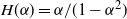 $H(\alpha ) = \alpha /(1 - {\alpha ^2})$
, using the terms through the second derivative gives
$H(\alpha ) = \alpha /(1 - {\alpha ^2})$
, using the terms through the second derivative gives
 \begin{align*}H(\alpha ) + \varepsilon H'(\alpha ) &+ {\varepsilon ^2}H''(\alpha )/2\\ &= H(\alpha ) + \varepsilon \left( {\alpha H(\alpha ) + 1} \right) + {\varepsilon ^2}\left( {\left( {1 + {\alpha ^2}} \right)H(\alpha ) + \alpha } \right)/2\\&= H(\alpha )\left\{ {1 + \varepsilon \left( {\alpha + (1 - {\alpha ^2})/\alpha } \right) + {\varepsilon ^2}\left( {\left( {1 + {\alpha ^2}} \right) + (1 - {\alpha ^2})} \right)/2} \right\}\\ &= H(\alpha )\left\{ {1 + \varepsilon /\alpha + {\varepsilon ^2}} \right\}.\end{align*}
For the third derivative term, we just want to bound it. Section 3 noted all derivatives of H are positive, so for
 $\varepsilon \le 0$
,
$\varepsilon \le 0$
,
 ${\varepsilon ^3}H'''(z) \le 0$
. For
${\varepsilon ^3}H'''(z) \le 0$
. For
 $\varepsilon > 0$
,
$\varepsilon > 0$
,
 ${\varepsilon ^3}H'''(z) \le {\varepsilon ^3}H'''(\alpha + \varepsilon )$
, and also, since
${\varepsilon ^3}H'''(z) \le {\varepsilon ^3}H'''(\alpha + \varepsilon )$
, and also, since
 $H'$
is increasing,
$H'$
is increasing,
 $H(\alpha + \varepsilon )$
 $ \le H(\alpha ) + \varepsilon H'(\alpha + \varepsilon )$
 $ = H(\alpha ) + \varepsilon \left( {(\alpha + \varepsilon )H(\alpha + \varepsilon ) + \alpha + \varepsilon } \right)$
. Solving,
$ = H(\alpha ) + \varepsilon \left( {(\alpha + \varepsilon )H(\alpha + \varepsilon ) + \alpha + \varepsilon } \right)$
. Solving,
 $H(\alpha + \varepsilon )$
 $ \le H(\alpha )\left( {\alpha + \varepsilon (1 - {\alpha ^2})} \right)\left( {1 - \varepsilon (\alpha + \varepsilon )} \right)$
 $ \le 1.0152H(\alpha )$
assuming
$ \le 1.0152H(\alpha )$
assuming
 $b > 1600$
so that
$b > 1600$
so that
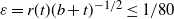 $\varepsilon = r(t){(b + t)^{ - 1/2}} \le 1/80$
. Then from (3.3),
$\varepsilon = r(t){(b + t)^{ - 1/2}} \le 1/80$
. Then from (3.3),
 \begin{align*}H'''(\alpha + \varepsilon )\le\left\{ {\left( {3(\alpha + \varepsilon ) + {{(\alpha + \varepsilon )}^3}} \right)(1.0152) + \left( {2 + {{(\alpha + \varepsilon )}^2}} \right)/H(\alpha )} \right\}H(\alpha ) \le 4.2H(\alpha ).\end{align*}
Thus
 \begin{align*}H(\alpha + \varepsilon ) &= H(\alpha ) + \varepsilon H'(\alpha ) + \frac{{{\varepsilon ^2}}}{2}H''(\alpha ) + \frac{{{\varepsilon ^3}}}{6}H'''(z) \le H(\alpha )\left\{ {1 + \frac{\varepsilon }{\alpha } + {\varepsilon ^2} + .7{{\left| \varepsilon \right|}^3}} \right\}\\&\le \frac{\alpha }{{1 - {\alpha ^2}}}\left\{ {\frac{{\alpha \sqrt {b + t} + r(t)}}{{\alpha \sqrt {b + t} }} + \frac{1}{{4(b + t)}} + \frac{{.7}}{{8{{(b + t)}^{3/2}}}}} \right\}\end{align*}
 \begin{align*}&\le \frac{\alpha }{{1 - {\alpha ^2}}}\frac{{\alpha \sqrt {b + t} + r(t)}}{{\alpha \sqrt {b + t} }}\left\{ {1 + \frac{{\alpha \sqrt {b + t} }}{{4(b + t)\left( {\alpha \sqrt {b + t} - 1/2} \right)}}\left( {1 + \frac{{.35}}{{{{(b + t)}^{1/2}}}}} \right)} \right\}\\&\le \frac{{\sqrt {b + t} }}{{1 - {\alpha ^2}}} {\frac{{W(t) + u}}{{b + t}}} \left\{ {1 + \frac{1}{{4b}}{{\left( {1 - \frac{1}{{2\alpha \sqrt b }}} \right)}^{ - 1}}\left( {1 + \frac{{.35}}{{\sqrt b }}} \right)} \right\}\\&\le \frac{{\sqrt {b + t} }}{{1 - {\alpha ^2}}} {\frac{{W(t) + u}}{{b + t}}} \left\{ {1 + \frac{1}{{4b}}\left( {1 + \frac{1}{{{b^{1/2}}}}} \right)} \right\},\text{using } b > 1600 \text{ in the last step}.\end{align*}
Referring back to (A.1),
 \begin{align*}V_{W}(u,b) &= (1-\alpha^2) \int_0^\infty {dF(t) (b + t)^{-1/2} H(\alpha + \varepsilon )} \\ &\le \int_0^\infty {dF(t)} {\dfrac{{W(t) + u}}{{b + t}}} \left\{ {1 + \dfrac{1}{{4b}}\left( {1 + \dfrac{1}{{\sqrt{b}}}} \right)} \right\}\\&= E\left[ {\dfrac{{W(T) + u}}{{b + T}}} \right]\left\{ {1 + \dfrac{1}{{4b}}\left( {1 +\dfrac{1}{{\sqrt{b}}}} \right)} \right\},\end{align*}
or
 \begin{equation}E\left[ {\frac{{W(T) + u}}{{b + T}}} \right]\left\{ {1 + \frac{1}{{4b}}\left( {1 + \frac{1}{{\sqrt{b}}}} \right)} \right\} \geqslant {V_W}(u,b).\end{equation}
Now embed the random walk in the Brownian motion as in Section 1.2, with
 ${S_n} = W({T_n})$
; whenever W(t) is an integer,
${S_n} = W({T_n})$
; whenever W(t) is an integer,
 $W(t) = W({T_n})$
for some n. For stop rule T, W(T) only takes integer values. Let
$W(t) = W({T_n})$
for some n. For stop rule T, W(T) only takes integer values. Let
 $n^*$
be the first n such that
$n^*$
be the first n such that
 $W(T) = W({T_n})$
.
$W(T) = W({T_n})$
.
 \begin{align*}&E\left[ {\frac{{W(T) + u}}{{b + T}}} \right] = \sum\limits_{n = 0}^\infty {E\left[ {\left. {\frac{{u + {S_n}}}{{b + n}}\frac{{b + n}}{{b + {T_n}}}} \right|{n^*} = n} \right]P({n^*} = n)}\\&= \sum\limits_{n = 0}^\infty {E\left[ {\frac{{b + n}}{{b + {T_n}}}} \right]E\left[ {\left. {\frac{{u + {S_n}}}{{b + n}}} \right|{n^*} = n} \right]P({n^*} = n)} \le \left( {1 + \frac{1}{{6b}}} \right)V(u,b),\end{align*}
using Lemma A.1. Combining with (A.2),
 \begin{align*}V(u,b) \ge {V_W}(u,b)\left( {1 - \frac{1}{{4b}}\left( {1 + \frac{1}{{\sqrt{b}}}} \right)} \right)\left( {1 - \frac{1}{{6b}}} \right) \ge {V_W}(u,b)\left( {1 - \frac{5}{{12b}}\left( {1 + \frac{1}{{{\sqrt{b}}}}} \right)} \right).\end{align*}
 \begin{align*}\text{REMARK. Numerical data suggests }V(u,b) \ge {V_W}(u,b)\left( {1 - \frac{1}{{4b}}\left( {1 + \frac{1}{{{\sqrt{b}}}}} \right)} \right).\end{align*}
Now the inequality
 $n{\left( {b + n} \right)^{ - 2}} \leqslant 1/(4b)$
used in proving Lemma A.1 is a gross overestimate when u is near the boundary
$n{\left( {b + n} \right)^{ - 2}} \leqslant 1/(4b)$
used in proving Lemma A.1 is a gross overestimate when u is near the boundary
 $\alpha \sqrt b $
, because in that case the time to crossing will probably be for n small compared to b. On the other hand, when u is far below
$\alpha \sqrt b $
, because in that case the time to crossing will probably be for n small compared to b. On the other hand, when u is far below
 $\alpha \sqrt b $
, our replacing
$\alpha \sqrt b $
, our replacing
 ${(b+t)^{ - 1}}/4$
by
${(b+t)^{ - 1}}/4$
by
 ${b^{ - 1}}/4$
in steps leading up to (A.2) is a significant overestimate, because t will be typically of order b in order to get to the boundary. But we will not pursue these things, because improving 5/12 to 1/4 in Lemma 1.2 would only slightly improve the lower estimate in Lemma 4.3, and the real goal is to prove Theorem 1.1.
${b^{ - 1}}/4$
in steps leading up to (A.2) is a significant overestimate, because t will be typically of order b in order to get to the boundary. But we will not pursue these things, because improving 5/12 to 1/4 in Lemma 1.2 would only slightly improve the lower estimate in Lemma 4.3, and the real goal is to prove Theorem 1.1.
Appendix B. Proof of Lemma 4.2
Proof of Lemma 4.2.
 $V(u - 2j + 1,b + 2n - 1) \le {V_W}(u - 2j + 1,b + 2n - 1)$
, and the displacement of
$V(u - 2j + 1,b + 2n - 1) \le {V_W}(u - 2j + 1,b + 2n - 1)$
, and the displacement of
 $u - 2j + 1$
from the Brownian boundary is
$u - 2j + 1$
from the Brownian boundary is
 \begin{align*}d&=u - 2j + 1 - \alpha \sqrt {b + 2n - 1}\\ &= u - 2j + 1 - \alpha \sqrt b \left( {1 + \dfrac{{2n - 1}}{{2b}}\left( {1 - \tau (n)\dfrac{{2n - 1}}{b}} \right)} \right)\\ &= - \left[ {2j - \left( {1 - \delta - \psi (n)} \right)} \right],\end{align*}
where
 $\psi (n) = \alpha \dfrac{{n - 1/2}}{{\sqrt b }}\left( {1 - \tau (n)\dfrac{{2n - 1}}{b}} \right), 0 < \tau (n) < 1/4.$
Now
$\psi (n) = \alpha \dfrac{{n - 1/2}}{{\sqrt b }}\left( {1 - \tau (n)\dfrac{{2n - 1}}{b}} \right), 0 < \tau (n) < 1/4.$
Now
 $\psi (n) \le {\alpha n}/{\sqrt b },$
and
$\psi (n) \le {\alpha n}/{\sqrt b },$
and
 $\psi (n) = {\alpha n}/{\sqrt b } - O({b^{ - 1/2 + 2p}}).$
Thus, from (3.7),
$\psi (n) = {\alpha n}/{\sqrt b } - O({b^{ - 1/2 + 2p}}).$
Thus, from (3.7),
 \begin{align}&{V_W}(u - 2j + 1,b + 2n - 1) \le \frac{{u - 2j + 1}}{{b + 2n - 1}} + \,\,\alpha \frac{{{{\left[ {2j - \left( {1 - \delta - \psi (n)} \right)} \right]}^2}}}{{{{\left( {b + 2n - 1} \right)}^{3/2}}}}\\ &\quad - \frac{{\left( {1 + {\alpha ^2}} \right)}}{3}\frac{{{{\left[ {2j - \left( {1 - \delta - \psi (n)} \right)} \right]}^3}}}{{{{\left( {b + 2n - 1} \right)}^2}}} + \frac{{\alpha \left( {4 + {\alpha ^2}} \right)}}{{12}}\frac{{{{\left[ {2j - \left( {1 - \delta - \psi (n)} \right)} \right]}^4}}}{{{{\left( {b + 2n - 1} \right)}^{5/2}}}}.\nonumber\end{align}
By (3.8), we get a lower bound for
 ${V_W}(u - 2j + 1,b + 2n - 1)$
by subtracting
${V_W}(u - 2j + 1,b + 2n - 1)$
by subtracting
 \begin{align*}\dfrac{{\left( {4 + 8{\alpha ^2} + {\alpha ^4}} \right)}}{{60}}\dfrac{{{{\left[ {2j - \left( {1 - \delta - \psi (n)} \right)} \right]}^5}}}{{{{\left( {b + 2n - 1} \right)}^3}}}\end{align*}
from this. To get
 $S_{RW}$
, these terms are to be weighted by
$S_{RW}$
, these terms are to be weighted by
 ${2^{ - 2n + 1}}B(n,j)$
and summed for j from 1 through n. But
${2^{ - 2n + 1}}B(n,j)$
and summed for j from 1 through n. But
 ${2^{ - 2n + 1}}\sum_{j = 1}^n {{j^5}B(n,j)} = O\left( {{n^2}} \right)$
, so this last term would add
${2^{ - 2n + 1}}\sum_{j = 1}^n {{j^5}B(n,j)} = O\left( {{n^2}} \right)$
, so this last term would add
 $O\left({n^2}{b^{-3}} \right) = O\left( {{b^{ - 2 + 2p}}} \right)$
, so the upper and lower bounds of the sum are the same to that order, and only involve the terms up through the fourth power of j. We break the sum into four pieces,
$O\left({n^2}{b^{-3}} \right) = O\left( {{b^{ - 2 + 2p}}} \right)$
, so the upper and lower bounds of the sum are the same to that order, and only involve the terms up through the fourth power of j. We break the sum into four pieces,
 $s_1,\ldots,s_4$
, corresponding to the four terms of the Taylor approximation on the right side of (B.1). The sums are done using (4.2) throughout. Some of the detail in obtaining the O bounds from the asserted bounds on n and
$s_1,\ldots,s_4$
, corresponding to the four terms of the Taylor approximation on the right side of (B.1). The sums are done using (4.2) throughout. Some of the detail in obtaining the O bounds from the asserted bounds on n and
 $\delta$
is left to the reader. Let
$\delta$
is left to the reader. Let
 \begin{align*}{s_1} &= {2^{ - 2n + 1}}\sum\limits_{j = 1}^n {B(n,j)\frac{{u - 2j + 1}}{{b + 2n - 1}}}\\&= \frac{{u + 1}}{{b + 2n - 1}}{2^{ - 2n + 1}}\sum\limits_{j = 1}^n {B(n,j)} - \frac{2}{{b + 2n - 1}}{2^{ - 2n + 1}}\sum\limits_{j = 1}^n {jB(n,j)} = \frac{{(u + 1){G_n} - 1}}{{b + 2n - 1}}\\ &= \frac{{(u + 1){G_n} - 1}}{b}\left( {1 - \frac{{2n - 1}}{b} + \frac{{{{(2n - 1)}^2}}}{{{b^2}}} + O({n^3}{b^{ - 3}})} \right)\\&= \frac{{(u + 1){G_n} - 1}}{b} - \frac{{(u + 1){G_n}}}{{{b^2}}}\left( {2n - 1 - \frac{{4{n^2}}}{b}} \right) + \frac{{2n}}{{{b^2}}} + O({b^{ - 2 + p}}). \end{align*}
The first term will conveniently cancel when we add to the leaf sum, so we leave that as is, but rewrite the second with
 $\delta$
rather than u as the variable:
$\delta$
rather than u as the variable:
 \begin{align*}& {s_1}- \frac{{(u + 1){G_n} - 1}}{b} = - \frac{{\alpha \sqrt b + 1 - \delta }}{{{b^2}}}\left( {2n{G_n} - {G_n} - 4\frac{{{n^2}{G_n}}}{b}} \right) + \frac{{2n}}{{{b^2}}} + O({b^{ - 2 + p}})\\ &= - \frac{\alpha }{{{b^{3/2}}}}\left( {1 + \frac{{1 - \delta }}{{\alpha \sqrt b }}} \right)\left( {2n{G_n} - {G_n} - 4\frac{{{n^2}{G_n}}}{b}} \right) + \frac{\alpha }{{{b^{3/2}}}}\frac{{2n}}{{\alpha \sqrt b }} + O({b^{ - 2 + p}}).\end{align*}
Simplifying,
 \begin{align}{s_1} - \frac{{(u + 1){G_n} - 1}}{b} &= \frac{\alpha }{{{b^{3/2}}}}\left\{ \begin{gathered} - 2n{G_n} + G_n + 2\frac{n}{{\alpha \sqrt b }} - 2\frac{{n{G_n}}}{{\alpha \sqrt b }} + 4\frac{{{n^2}{G_n}}}{b} \\ + 2\delta \left( {\frac{{n{G_n}}}{{\alpha \sqrt b }}} \right)+ O({b^{ -1/ 2 + p}}) \end{gathered} \right\}.\end{align}
Let
 $h = 1 - \delta - \psi (n)$
, to simplify the writing for the next three terms. Let
$h = 1 - \delta - \psi (n)$
, to simplify the writing for the next three terms. Let
 \begin{align*}{s_2} &= \frac{\alpha }{{{{\left( {b + 2n - 1} \right)}^{3/2}}}}{2^{ - 2n + 1}}\sum\limits_{j = 1}^n {B(n,j){{\left[ {2j - \left( {1 - \delta - \psi (n)} \right)} \right]}^2}}\\ & = \frac{\alpha }{{{b^{3/2}}}}\left( {1 - \frac{3}{2}\frac{{(2n - 1)}}{b} + O({b^{ - 1 + 2p}})} \right){2^{ - 2n + 1}}\sum\limits_{j = 1}^n {B(n,j)} \left[ {4{j^2} - 4jh + {h^2}} \right]\\ & = \frac{\alpha }{{{b^{3/2}}}}\left( {1 - \frac{{3n}}{b} + O({b^{ - 1 + 2p}})} \right)\left[ {4n{G_n} - 2h + {G_n}{h^2}} \right].\end{align*}
This can be arranged to give (recall
 $\psi (n) = {\alpha n}/{\sqrt b } - O({b^{ - 1/2 + 2p}})$
)
$\psi (n) = {\alpha n}/{\sqrt b } - O({b^{ - 1/2 + 2p}})$
)
 \begin{align}{s_2} &= \frac{\alpha }{{{b^{3/2}}}}\left\{ \begin{gathered} 4n{G_n} - 2 + 2\alpha \frac{n}{{\sqrt b }} + {G_n} - \left( {12 - {\alpha ^2}} \right)\frac{{{n^2}{G_n}}}{b} \\ - 2\alpha \frac{{n{G_n}}}{{\sqrt b }} + 2\delta \left( {1 - {G_n} + \alpha \frac{{n{G_n}}}{{\sqrt b }}} \right) + {\delta ^2}{G_n} + O({b^{ -1/ 2 + 2p}}) \\\end{gathered} \right\}.\end{align}
For the next two terms, note
 $h = O\left( {{b^p}} \right)$
to help simplify. Let
$h = O\left( {{b^p}} \right)$
to help simplify. Let
 \begin{align*}{s_3} &= - \frac{{(1 + {\alpha ^2})}}{{3{{\left( {b + 2n - 1} \right)}^2}}}{2^{ - 2n + 1}}\sum\limits_{j = 1}^n {B(n,j){{\left[ {2j - \left( {1 - \delta - \psi (n)} \right)} \right]}^3}}\\& = - \frac{{(1 + {\alpha ^2})}}{{3{b^2}}}\left( {1 - \frac{{4n}}{b} + O({b^{ - 1 + 2p}})} \right){2^{ - 2n + 1}}\sum\limits_{j = 1}^n {B(n,j)} \left[ {8{j^3} - 12{j^2}h + 6j{h^2} - {h^3}} \right]\\& = - \frac{\alpha }{{{b^{3/2}}}}\frac{{(1 + {\alpha ^2})}}{{3\alpha \sqrt b }}\left( {1 + O({b^{ - 1/2 + p}})} \right)\left[ {6n - 2 - 12n{G_n}h + 3{h^2} - {G_n}{h^3}} \right].\end{align*}
The
 ${h^2}$
and
${h^2}$
and
 ${h^3}$
terms contribute only
${h^3}$
terms contribute only
 $O({b^{ - 2 + 2p}})$
, so this becomes
$O({b^{ - 2 + 2p}})$
, so this becomes
 \begin{align}&{s_3} = \frac{\alpha }{{{b^{3/2}}}}\frac{{(1 + {\alpha ^2})}}{\alpha }\left\{ { - \frac{2n}{{\sqrt b }} + \frac{{4n{G_n}}}{{\sqrt b }} - \frac{4\alpha{{n^2}{G_n}}}{b} - \delta \left( {\frac{{4n{G_n}}}{{\sqrt b }}} \right)} + O({b^{ -1/2 + 2p}}) \right \}.\end{align}
Let
 \begin{align*}{s_4} &= \frac{{\alpha (4 + {\alpha ^2})}}{{12{{\left( {b + 2n - 1} \right)}^{5/2}}}}{2^{ - 2n + 1}}\sum\limits_{j = 1}^n {B(n,j){{\left[ {2j - \left( {1 - \delta - \psi (n)} \right)} \right]}^4}} \\&= \frac{{\alpha (4 + {\alpha ^2})}}{{12{b^{5/2}}}}\left( {1 + O({b^{ - 1/2 + p}})} \right){2^{ - 2n + 1}}\sum\limits_{j = 1}^n {B(n,j)} \left[ \begin{gathered} 16{j^4} - 32{j^3}h \\ + 24{j^2}{h^2} - 8j{h^3} + {h^4} \\\end{gathered} \right]\\&= \frac{\alpha }{{{b^{3/2}}}}\frac{{(4 + {\alpha ^2})}}{{12b}}\left( {1 + O({b^{ - 1/2 + p}})} \right)\left[ \begin{gathered} 16n(2n - 1){G_n} - 8(3n - 1)h \\ + 24n{G_n}{h^2} - 4{h^3} + {G_n}{h^4} \\\end{gathered} \right].\end{align*}
This reduces to
 \begin{align}{s_4} &= \frac{\alpha }{{{b^{3/2}}}}\left\{ {\frac{{8(4 + {\alpha ^2})}}{3}\frac{{{n^2}{G_n}}}{b}} + O({b^{ -1/2 + 2p}}) \right \}.\end{align}
Combining (B.2) through (B.5),
 \begin{align*} {S_{RW}} - \dfrac{{(u + 1){G_n} - 1}}{b}=\frac{\alpha }{b^{3/2}}\left\{ \begin{gathered} 2n{G_n}- 2+2G_n+2(\alpha+1/\alpha)\frac{{n{G_n}}}{{\sqrt b }} - \frac{{{(4+\alpha ^2)}}}{3}\frac{{n^2}{G_n}}{b} \\ + 2\delta \left( {1 - {G_n} - (\alpha+1/\alpha) \frac{{n{G_n}}}{{\sqrt b }}} \right) + {\delta ^2}{G_n} + O({b^{ - 1/2 + 2p}}) \\\end{gathered} \right\}.\end{align*}
Appendix C. Proof of Theorem 5.1
Proof of Theorem 5.1. The proof is by induction. The case
 $j=0$
is (5.1). The base case for the induction proof is
$j=0$
is (5.1). The base case for the induction proof is
 $j = 1$
, which was done at (5.4). Assume true for
$j = 1$
, which was done at (5.4). Assume true for
 $j$
, show true for
$j$
, show true for
 $j + 1$
. That is, assume formula is true for
$j + 1$
. That is, assume formula is true for
 $j - 1/2 \le \delta \le j + 1/2$
. Continue to use
$j - 1/2 \le \delta \le j + 1/2$
. Continue to use
 $n = \lfloor {\sqrt b /2}\rfloor $
. Now consider
$n = \lfloor {\sqrt b /2}\rfloor $
. Now consider
 $j + 1/2 \le \delta \le j + 3/2$
. Break the proof into cases.
$j + 1/2 \le \delta \le j + 3/2$
. Break the proof into cases.
Case (a):
 $j + 1/2 \le \delta \le j + 1$
. We need to estimate
$j + 1/2 \le \delta \le j + 1$
. We need to estimate
 $V(u + 1,b + 2m + 1)$
for
$V(u + 1,b + 2m + 1)$
for
 $0 \le m < n$
. From (5.2), the distance of
$0 \le m < n$
. From (5.2), the distance of
 $u + 1$
from boundary is
$u + 1$
from boundary is
 $d = \alpha m{b^{ - 1/2}} + \delta - 1 + {L^ + }\left( {\alpha {b^{ - 1/2}}/2} \right)$
, so
$d = \alpha m{b^{ - 1/2}} + \delta - 1 + {L^ + }\left( {\alpha {b^{ - 1/2}}/2} \right)$
, so
 $\alpha m{b^{ - 1/2}} + j - 1/2 \le \alpha m{b^{ - 1/2}} + \delta - 1 + {L^ + }\left( {\alpha {b^{ - 1/2}}/2} \right) \le \alpha m{b^{ - 1/2}} + j + {L^ + }\left( {\alpha {b^{ - 1/2}}/2} \right)$
. Thus for
$\alpha m{b^{ - 1/2}} + j - 1/2 \le \alpha m{b^{ - 1/2}} + \delta - 1 + {L^ + }\left( {\alpha {b^{ - 1/2}}/2} \right) \le \alpha m{b^{ - 1/2}} + j + {L^ + }\left( {\alpha {b^{ - 1/2}}/2} \right)$
. Thus for
 $0 \le m < n \le \sqrt b /2$
, we have
$0 \le m < n \le \sqrt b /2$
, we have
 $j - 1/2 \le d \le j + \alpha /2 + {L^ + }\left( {\alpha {b^{ - 1/2}}/2} \right) < j + 1/2$
since
$j - 1/2 \le d \le j + \alpha /2 + {L^ + }\left( {\alpha {b^{ - 1/2}}/2} \right) < j + 1/2$
since
 $b \ge {b_0},$
so the induction hypothesis applies with d in the place of
$b \ge {b_0},$
so the induction hypothesis applies with d in the place of
 $\delta$
, and
$\delta$
, and
 $b + 2m + 1$
in the place of b. So
$b + 2m + 1$
in the place of b. So
 ${V_E}(u + 1,b + 2m + 1) = \alpha {(b + 2m + 1)^{ - 3/2}}\left\{{2j\left( {d - 1/2} \right) - j(j - 1) + L({M_j}{b^{ - 1/4}})} \right\}.$
But
${V_E}(u + 1,b + 2m + 1) = \alpha {(b + 2m + 1)^{ - 3/2}}\left\{{2j\left( {d - 1/2} \right) - j(j - 1) + L({M_j}{b^{ - 1/4}})} \right\}.$
But
 $\alpha {(b+ 2m+ 1)^{- 3/2}} = \alpha {b^{- 3/2}}\left({1 - {L^+}(1.5{b^{- 1/2}})} \right),$
and
$\alpha {(b+ 2m+ 1)^{- 3/2}} = \alpha {b^{- 3/2}}\left({1 - {L^+}(1.5{b^{- 1/2}})} \right),$
and
 $2j\left({d - 1/2} \right) - j(j-1) \le {j^2} + j.$
Using
$2j\left({d - 1/2} \right) - j(j-1) \le {j^2} + j.$
Using
 $j \le {b^{1/10}}$
and
$j \le {b^{1/10}}$
and
 $b \ge {b_0}$
,
$b \ge {b_0}$
,
 ${V_E}(u + 1,b + 2m + 1) = \alpha {b^{ - 3/2}}\left\{ {2j\left( {\alpha m{b^{ - 1/2}} + \delta - 3/2} \right) - j(j - 1) + L\left( {({M_j} + 2){b^{ - 1/4}}} \right)} \right\}$
. So
${V_E}(u + 1,b + 2m + 1) = \alpha {b^{ - 3/2}}\left\{ {2j\left( {\alpha m{b^{ - 1/2}} + \delta - 3/2} \right) - j(j - 1) + L\left( {({M_j} + 2){b^{ - 1/4}}} \right)} \right\}$
. So
 $\alpha^{-1} {b^{ 3/2}}{S_{LE}} = \sum\limits_{m = 0}^{n - 1} {{2^{ - 2m - 1}}{C_m}\left\{ {\left( {2j\left( {\alpha m{b^{ - 1/2}} + \delta - 3/2} \right) - j(j - 1) + L\left( {({M_j} + 2){b^{ - 1/4}}} \right)} \right)} \right\}}=( n{G_n} - 1 +\! {G_n} ) 2j\alpha {b^{ - 1/2}} + \left( {2j(\delta - 3/2) - j(j - 1)} \right)\left( {1 - {G_n}} \right) + L\left( {({M_j} + 2){b^{ - 1/4}}} \right).$
But
$\alpha^{-1} {b^{ 3/2}}{S_{LE}} = \sum\limits_{m = 0}^{n - 1} {{2^{ - 2m - 1}}{C_m}\left\{ {\left( {2j\left( {\alpha m{b^{ - 1/2}} + \delta - 3/2} \right) - j(j - 1) + L\left( {({M_j} + 2){b^{ - 1/4}}} \right)} \right)} \right\}}=( n{G_n} - 1 +\! {G_n} ) 2j\alpha {b^{ - 1/2}} + \left( {2j(\delta - 3/2) - j(j - 1)} \right)\left( {1 - {G_n}} \right) + L\left( {({M_j} + 2){b^{ - 1/4}}} \right).$
But
 $0 \le ( n{G_n} - 1 + {G_n} ) 2j\alpha {b^{ - 1/2}} \le \alpha j{b^{ - 1/4}},$
and
$0 \le ( n{G_n} - 1 + {G_n} ) 2j\alpha {b^{ - 1/2}} \le \alpha j{b^{ - 1/4}},$
and
 $0 \ge - \left( {2j(\delta - 3/2) - j(j - 1)} \right){G_n} \ge - {j^2}{b^{ - 1/4}},$
and
$0 \ge - \left( {2j(\delta - 3/2) - j(j - 1)} \right){G_n} \ge - {j^2}{b^{ - 1/4}},$
and
 ${j^2} \ge \alpha j$
, so
${j^2} \ge \alpha j$
, so
 $\alpha^{-1} {b^{ 3/2}}{S_{LE}} = {\left( {2j(\delta - 3/2) - j(j - 1)} \right) + L\left( {\left( {{M_j} + {j^2} + 2} \right){b^{ - 1/4}}} \right)}.$
From Lemma 5.1, to get
$\alpha^{-1} {b^{ 3/2}}{S_{LE}} = {\left( {2j(\delta - 3/2) - j(j - 1)} \right) + L\left( {\left( {{M_j} + {j^2} + 2} \right){b^{ - 1/4}}} \right)}.$
From Lemma 5.1, to get
 $\alpha^{-1} {b^{ 3/2}}{V_E}$
, add this to
$\alpha^{-1} {b^{ 3/2}}{V_E}$
, add this to
 ${2(\delta - 1/2) + L({\delta ^2}{b^{ - 1/4}})}.$
Noting
${2(\delta - 1/2) + L({\delta ^2}{b^{ - 1/4}})}.$
Noting
 $\delta \le j + 1$
, this gives
$\delta \le j + 1$
, this gives
 \begin{align}\frac{{b^{ 3/2}}}{\alpha}{V_E}(u,b) = {\left( {2(j + 1)(\delta - 1/2) - j(j + 1)} \right) + L\left( {({M_j} + 2{j^2} + 2j + 3){b^{ - 1/4}}} \right)} .\end{align}
Case (b):
 $j + 1 \le \delta \le j + 3/2$
. Let
$j + 1 \le \delta \le j + 3/2$
. Let
 ${m_0} = \min \left\{ {\left\lfloor {\frac{{j + 3/2 - \delta }}{\alpha }\sqrt b } \right\rfloor ,n} \right\}$
. Break m into ranges.
${m_0} = \min \left\{ {\left\lfloor {\frac{{j + 3/2 - \delta }}{\alpha }\sqrt b } \right\rfloor ,n} \right\}$
. Break m into ranges.
Range (i): For
 $0 \le m \le {m_0} - 1$
,
$0 \le m \le {m_0} - 1$
,
 $\alpha m{b^{ - 1/2}} \le \alpha {m_0}{b^{ - 1/2}} - \alpha {b^{ - 1/2}} \le j + 3/2 - \delta - \alpha {b^{ - 1/2}}$
, so
$\alpha m{b^{ - 1/2}} \le \alpha {m_0}{b^{ - 1/2}} - \alpha {b^{ - 1/2}} \le j + 3/2 - \delta - \alpha {b^{ - 1/2}}$
, so
 $d = \alpha m{b^{ - 1/2}} + \delta - 1 + {L^ + }\left( {\alpha {b^{ - 1/2}}/2} \right) \le j + 3/2 - \delta - \alpha {b^{ - 1/2}} + \delta - 1 + {L^ + }\left( {\alpha {b^{ - 1/2}}/2} \right) \le j + 1/2$
, so the induction hypothesis applies with d in place of
$d = \alpha m{b^{ - 1/2}} + \delta - 1 + {L^ + }\left( {\alpha {b^{ - 1/2}}/2} \right) \le j + 3/2 - \delta - \alpha {b^{ - 1/2}} + \delta - 1 + {L^ + }\left( {\alpha {b^{ - 1/2}}/2} \right) \le j + 1/2$
, so the induction hypothesis applies with d in place of
 $\delta $
and
$\delta $
and
 $b + 2m + 1$
in place of b. The same argument that was used in (a) then shows
$b + 2m + 1$
in place of b. The same argument that was used in (a) then shows
 ${V_E}(u + 1,b + 2m + 1) = \alpha {b^{ - 3/2}}\left\{ {2j\left( {\alpha m{b^{ - 1/2}} + \delta - 3/2} \right) - j(j - 1) + L\left( {({M_j} + 2){b^{ - 1/4}}} \right)} \right\}.$
Range (ii): Suppose
 ${m_0} + 1 \le m < n$
(this could be empty). Then
${m_0} + 1 \le m < n$
(this could be empty). Then
 $m \ge {m_0} + 1 \ge \frac{{j + 3/2 - \delta }}{\alpha }\sqrt b $
, so
$m \ge {m_0} + 1 \ge \frac{{j + 3/2 - \delta }}{\alpha }\sqrt b $
, so
 $d = \alpha m{b^{ - 1/2}} + \delta - 1 + {L^ + }\left( {\alpha {b^{ - 1/2}}/2} \right) \ge j + 3/2 - \delta + \delta - 1 + {L^ + }\left( {\alpha {b^{ - 1/2}}/2} \right) \ge j + 1/2$
. And
$d = \alpha m{b^{ - 1/2}} + \delta - 1 + {L^ + }\left( {\alpha {b^{ - 1/2}}/2} \right) \ge j + 3/2 - \delta + \delta - 1 + {L^ + }\left( {\alpha {b^{ - 1/2}}/2} \right) \ge j + 1/2$
. And
 $\alpha m{b^{ - 1/2}} + \delta - 1 + {L^ + }\left( {\alpha {b^{ - 1/2}}/2} \right) \le \alpha /2 + j + 1/2 + {L^ + }\left( {\alpha {b^{ - 1/2}}/2} \right) \le j + 1$
for
$\alpha m{b^{ - 1/2}} + \delta - 1 + {L^ + }\left( {\alpha {b^{ - 1/2}}/2} \right) \le \alpha /2 + j + 1/2 + {L^ + }\left( {\alpha {b^{ - 1/2}}/2} \right) \le j + 1$
for
 $b \ge {b_0}$
. Thus (C.1) applies with d in place of
$b \ge {b_0}$
. Thus (C.1) applies with d in place of
 $\delta $
and
$\delta $
and
 $b + 2m + 1$
in place of b. Using the asserted bounds and arguments similar to those in used in (a) leads to
$b + 2m + 1$
in place of b. Using the asserted bounds and arguments similar to those in used in (a) leads to
 ${V_E}(u + 1,b + 2m + 1) = \alpha {b^{ - 3/2}}\left\{ {2(j + 1)\left( {\alpha m{b^{ - 1/2}} + \delta - 3/2} \right) - j(j + 1) + L\left( {\left( {{M_j} + 2{j^2} + 2j + 6} \right){b^{ - 1/4}}} \right)} \right\}.$
Range (iii): For
 $m = {m_0}$
, either
$m = {m_0}$
, either
 $d \le 1/2$
or
$d \le 1/2$
or
 $d \ge 1/2$
, so one of the two formulas applies. But
$d \ge 1/2$
, so one of the two formulas applies. But
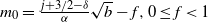 ${m_0} = \frac{{j + 3/2 - \delta }}{\alpha }\sqrt b - f,0 \le f < 1$
, so
${m_0} = \frac{{j + 3/2 - \delta }}{\alpha }\sqrt b - f,0 \le f < 1$
, so
 $\alpha {m_0}{b^{ - 1/2}} - 3/2 + \delta = j - \alpha f{b^{ - 1/2}}$
, so
$\alpha {m_0}{b^{ - 1/2}} - 3/2 + \delta = j - \alpha f{b^{ - 1/2}}$
, so
 $2j\left( {\alpha {m_0}{b^{ - 1/2}} + \delta - 3/2} \right) - j(j - 1) = 2(j + 1)\left( {\alpha {m_0}{b^{ - 1/2}} + \delta - 3/2} \right) - j(j + 1) + 2\alpha f{b^{ - 1/2}},$
which differ by only
$2j\left( {\alpha {m_0}{b^{ - 1/2}} + \delta - 3/2} \right) - j(j - 1) = 2(j + 1)\left( {\alpha {m_0}{b^{ - 1/2}} + \delta - 3/2} \right) - j(j + 1) + 2\alpha f{b^{ - 1/2}},$
which differ by only
 $2\alpha f{b^{ - 1/2}}.$
We can use the formula from (ii) for
$2\alpha f{b^{ - 1/2}}.$
We can use the formula from (ii) for
 $m = {m_0}$
regardless, and the result is the same, since
$m = {m_0}$
regardless, and the result is the same, since
 $({M_j} + 2){b^{ - 1/4}} + 2\alpha f{b^{ - 1/2}} = L\left( {\left( {{M_j} + 2{j^2} + 2j + 6} \right){b^{ - 1/4}}} \right).$
Summing over the formulas for ranges (i)–(iii),
 \begin{align*}\alpha^{-1}{b^{ 3/2}}{S_{LE}} &=\sum\limits_{m = 0}^{{m_0} - 1} {{2^{ - 2m - 1}}{C_m}}\left( \begin{array}{l}2j\left( {\alpha m{b^{ - 1/2}} + \delta - 3/2} \right) - j(j - 1)\\ + L\left( {{(M_j + 2)}{b^{ - 1/4}}} \right)\end{array} \right)\\&\quad + \sum\limits_{m = {m_0}}^{n - 1} {{2^{ - 2m - 1}}{C_m}}\left( \begin{array}{l}2(j + 1)\left( {\alpha m{b^{ - 1/2}} + \delta - 3/2} \right) - j(j + 1)\\ + L\left( {\left( {{M_j} + 2{j^2} + 2j + 6} \right){b^{ - 1/4}}} \right)\end{array} \right).\end{align*}
The error terms can be gotten out of the sum since
 $\sum_{m = 0}^n {{2^{ - 2m - 1}}{C_m}} < 1.$
Algebra gives
$\sum_{m = 0}^n {{2^{ - 2m - 1}}{C_m}} < 1.$
Algebra gives
 $\alpha^{-1}{b^{ 3/2}}{S_{LE}} =2\alpha {b^{ - 1/2}}\left(j\left({n{G_n} - 1 + {G_n}} \right)\sum\limits_{m = {m_0}}^{n - 1} {{2^{ - 2m - 1}}{C_m}m} + 2\left( {\delta - j - 3/2} \right)({G_{{m_0}}} - {G_n}) \right) + \left( {2j\left( {\delta - 1/2} \right) - j(j + 1)} \right)\left( {1 - {G_n}} \right)+ L\left( {\left( {{M_j} + 2{j^2} + 2j + 6} \right){b^{ - 1/4}}} \right).$
Estimating terms,
$\alpha^{-1}{b^{ 3/2}}{S_{LE}} =2\alpha {b^{ - 1/2}}\left(j\left({n{G_n} - 1 + {G_n}} \right)\sum\limits_{m = {m_0}}^{n - 1} {{2^{ - 2m - 1}}{C_m}m} + 2\left( {\delta - j - 3/2} \right)({G_{{m_0}}} - {G_n}) \right) + \left( {2j\left( {\delta - 1/2} \right) - j(j + 1)} \right)\left( {1 - {G_n}} \right)+ L\left( {\left( {{M_j} + 2{j^2} + 2j + 6} \right){b^{ - 1/4}}} \right).$
Estimating terms,
 \begin{align*}&2j\alpha {b^{ - 1/2}}\left( {n{G_n} - 1 + {G_n}} \right) \le 2j\alpha (2/n)n{G_n} \le j\alpha \sqrt {2.14/\pi } {b^{ - 1/4}},\\&\left( {2j\left( {\delta - 1/2} \right) - j(j + 1)} \right){G_n} \le ({j^2} + j){G_n} \le ({j^2} + j)\sqrt {2.14/\pi } {b^{ - 1/4}},\\&2\alpha {b^{ - 1/2}}\sum\limits_{m = {m_0}}^{n - 1} {{2^{ - 2m - 1}}{C_m}m} \le 2\alpha {b^{ - 1/2}}(n{G_n}) \le \alpha \sqrt {2/\pi } {b^{ - 1/4}},\\&2\left( {j + 3/2 - \delta } \right)({G_{{m_0}}} - {G_n}) \le 2\alpha {b^{ - 1/2}}\left( {{m_0} + 1} \right){G_{{m_0}}} \le 2\alpha {b^{ - 1/2}}n{G_n} + 2\alpha {b^{ - 1/2}}\end{align*}
(because
 $m{G_m}$
is an increasing function), so
$m{G_m}$
is an increasing function), so
 $2\left( {j + 3/2 - \delta } \right)({G_{{m_0}}} - {G_n}) \le \alpha \sqrt {2/\pi } {b^{ - 1/4}} + 2\alpha {b^{ - 1/2}} = L\left( {{b^{ - 1/4}}} \right).$
Using these estimates,
$2\left( {j + 3/2 - \delta } \right)({G_{{m_0}}} - {G_n}) \le \alpha \sqrt {2/\pi } {b^{ - 1/4}} + 2\alpha {b^{ - 1/2}} = L\left( {{b^{ - 1/4}}} \right).$
Using these estimates,
 \begin{align*}{S_{LE}} = \alpha {b^{ - 3/2}}\left\{ {2j\left( {\delta - 1/2} \right) - j(j + 1) + L\left( {\left( {{M_j} + 3{j^2} + 4j + 8} \right){b^{ - 1/4}}} \right)} \right\}.\end{align*}
Add this to
 $\alpha {b^{ - 3/2}}\left( {2(\delta - 1/2) + L({\delta ^2}{b^{ - 1/4}})} \right)$
from Lemma 5.1, using
$\alpha {b^{ - 3/2}}\left( {2(\delta - 1/2) + L({\delta ^2}{b^{ - 1/4}})} \right)$
from Lemma 5.1, using
 $\delta \le j + 3/2$
, to get
$\delta \le j + 3/2$
, to get
 ${V_E}(u,b) = \dfrac{\alpha }{{{b^{3/2}}}}\left\{ {\left( {2(j + 1)(\delta - 1/2) - j(j + 1)} \right) + L\left( {\left( {{M_j} + 4{j^2} + 7j + 11} \right){b^{ - 1/4}}} \right)} \right\},$
valid over the range
${V_E}(u,b) = \dfrac{\alpha }{{{b^{3/2}}}}\left\{ {\left( {2(j + 1)(\delta - 1/2) - j(j + 1)} \right) + L\left( {\left( {{M_j} + 4{j^2} + 7j + 11} \right){b^{ - 1/4}}} \right)} \right\},$
valid over the range
 $j + 1/2 \le \delta \le j + 3/2$
, and the induction proof is complete, upon letting
$j + 1/2 \le \delta \le j + 3/2$
, and the induction proof is complete, upon letting
 ${M_{j + 1}} = {M_j} + 4{j^2} + 7j + 11$
. This recursion, with
${M_{j + 1}} = {M_j} + 4{j^2} + 7j + 11$
. This recursion, with
 ${M_1} = 5$
, is easily seen to imply
${M_1} = 5$
, is easily seen to imply
 ${M_j} \le 5{j^3}$
. Of course a much smaller upper bound on
${M_j} \le 5{j^3}$
. Of course a much smaller upper bound on
 ${M_j}$
is possible.
${M_j}$
is possible.
Acknowledgements
We thank T. P. Hill for introducing us to this problem, and for pointing out the work of Häggström and Wästlund, which motivated what we did. We also thank him for discussions and encouragement about what we were doing, which was much needed lest we give up when the algebra seemed hopeless. We also thank Doron Zeilberger for encouragement and inspiration. We thank Steve Mann for supplying the fast Intel MMX code for both floating and integer 128-bit arithmetic that was needed for the rigorous determination of stop rules for the extremely large number of flips considered. We thank Donald Knuth for a helpful discussion about the asymptotic notation used.
Funding information
There are no funding bodies to thank relating to the creation of this paper.
Competing interests
There were no competing interests to declare which arose during the preparation or publication process of this paper.


 Open access