Shedding light on Swiss health insurance costs in the last year of life

Abstract

Healthcare costs tend to increase with age. In particular, in the case of illness, the last year before death can be an exceptionally costly period as the need for healthcare increases. Using a novel private insurance dataset containing over one million records of claims submitted by individuals to their health insurance providers during the last year of life, our research seeks to shed light on the costs before death in Switzerland. Our work documents how spending patterns change with proximity to dying. We use machine learning algorithms to identify and quantify the key effects that drive a person’s spending during this critical period. Our findings provide a more profound understanding of the costs associated with hospitalization before death, the role of age, and the variation in costs based on the services, including care services, which individuals require.

1. Introduction

Individual healthcare costs vary over a lifetime. In Switzerland, for example, the net costs per insured person significantly increase from age 45 (Federal Office of Public Health, 2022). Similarly, research suggests that healthcare spending increases after age 50, and attention is usually focused on the last months of life as they tend to be more costly (Alemayehu & Warner, 2004; Felder et al., 2000; Ladusingh & Pandey, 2013). In this sense, French et al. (2017) find that high medical expenses are documented shortly before death in different healthcare systems. For example, it has been estimated that between 8% and 11% of all healthcare expenses correspond to the tiny share of those who die (Polder et al., 2006; Sallnow et al., 2022). More extreme results have been observed in the United States, where it was estimated that 5.1% of deaths under Medicare accounted for 29.1% of total payments (Zweifel et al., 1999) and where significant costs may be paid by the patients as out-of-pocket expenditures (Kelley et al., 2013). However, some claim that these high costs may be influenced by excessive medical intervention in the final months, which can increase bills and suffering without much benefit (Diernberger et al., 2021; Luta et al., 2020; Sallnow et al., 2022). It is often questioned how palliative care could provide cheaper help while improving the quality of life in the last months (Sallnow et al., 2022), while some point out that current strategies lead to people spending too much time in hospitals when they would prefer to be cared for at home (Luta et al., 2020).

The main objective of this research is to shed light on insurance claims that arise from mandatory health insurance coverage ¹ in the last year of life in Switzerland. We study the main influencing factors, including demographic characteristics and those related to the types of healthcare services received. Focusing on the 12 twelve months of life is a common practice (see, e.g., Diernberger et al., 2021; Duncan et al., 2019; Luta et al., 2020; Panczak et al., 2017; Polder et al., 2006) and gives a view of the expenses over this critical period. ² In this work, we will use the shorthand term “cost of dying” or “cost of end-of-life care” to refer to the total health insurance claims during the last year of life.

Given the context of increasing healthcare costs, a more profound understanding of how many resources are spent on the various healthcare services by the dying is relevant to insurers and policymakers. For instance, in the case of the United States, Duncan et al. (2019) state that “patients at end of life (EOL) represent a disproportionate share of Medicare’s costs, implying that these patients are an appropriate population for management.” In this sense, entities such as governments or insurance companies that share the risk associated with these expenses will benefit from a greater understanding of the dynamics behind EOL expenses, which will better enable them to identify areas to reduce costs and incentivize alternatives that improve the quality of life during the patients’ last months. This is essential when deciding whether the level of expenses can be considered adequate. Results help to uncover the consequences of healthcare decision-making patterns and to optimize the structure of financing future healthcare expenses given the current cost dynamics. Society evolves, and so does how people die. This is particularly true in the current demographic context with aging populations in industrialized countries, threatening to alter the patterns of illness and death (Bone et al., 2018). For example, Stucki (2021) notes that the demographic transition in Switzerland “came with changing morbidity patterns.” Overall, authorities in many countries can now expect to see citizens dying at older ages and living a prolonged dying process (Sallnow et al., 2022). This could put pressure on institutions for older people as resources tend to “shift from medical cure to social care” (Payne et al., 2009). In this sense, recent research suggests that the future may be characterized by many more deaths occurring in nursing homes, hospices, and private homes (Bone et al., 2018; Thomas, 2021). Some countries are already experiencing this shift. In the Netherlands, for example, French et al. (2017) state that about 50% of spending in the last year of life corresponds to long-term care (LTC) services, as hospital spending is rather “modest.”

Access to healthcare, and therefore its cost and utilization, can be influenced by many factors. These factors may translate into different care costs at the EOL. For example, Diernberger et al. (2021) state that living in large urban areas results in people using more healthcare. Ladusingh and Pandey (2013) reach a similar conclusion for India. The disease affecting the individual is also expected to play a role in the cost of dying, as is the age at death (Felder et al., 2000; Luta et al., 2020; Panczak et al., 2017; Polder et al., 2006; Scitovsky, 1994). Moreover, the proximity to death is typically critical, as treatments tend to intensify in the last days of life (French et al., 2017; Luta et al., 2020; Martín et al., 2011; Zweifel et al., 1999). Particular attention has been paid to the last three months, which are considered essential. For example, in countries such as the United States, it was once estimated that half of all healthcare costs were incurred in the last 60 days of life (Scitovsky, 1994). For the case of Switzerland, however, Felder et al. (2000) found that the increase in expenses during the last months of life was not as extreme as in the United States. The role of gender is still not obvious. Some find that healthcare use and costs are higher for men (see, e.g., Luta et al., 2020, and Diernberger et al., 2021). Conversely, Polder et al. (2006) state that gender differences in healthcare costs in the last year of life are “small” and “statistically not significant.” In contrast, the need for hospitalization is a major trigger for the costs of dying. Luta et al. (2020) find that hospital costs may account for “most end-of-life care costs.” Ladusingh and Pandey (2013) find that in the case of India, costs tend to be particularly high when longer hospital stays are required.

To assess what factors may play a role in the value of claims related to EOL healthcare in Switzerland, we draw on a private dataset containing over one million records of claims submitted by individuals to their mandatory health insurer during the last year of their lives. This dataset contains information for 13 years from 2008 to 2020 and accumulates the costs associated with $30,800$ deaths. We analyze the data using regression, random forest (RF), and gradient boosting machine (GBM) models, retaining GBMs for our final model. We first assess the available covariates’ importance and then estimate the effect of the relevant variables using partial dependence (PD) coefficients. We conclude that the costs of dying in Switzerland are mainly driven by the number of days individuals are hospitalized, as well as by the number of consultations required, the age of the decedent at death, the proportion of costs incurred in the last three months of life, and the total length of treatment. In addition, we show how spending patterns vary based on the patients’ main expense category and the proximity to death.

The paper is organized as follows: Section 2 begins by providing the information available for our analysis and presents descriptive statistics on the data. Section 3 introduces the methodological details, and Section 4 discloses the main results of the model. We finish with our conclusions in Section 5 and provide additional details in the Appendix.

2. Available data and descriptive statistics

Our database consists of $1,262,686$ records associated with claims submitted by $30,800$ individuals during the last year of their lives to their mandatory health insurance provider between 2008 and 2020. These private data have been provided to us by a Swiss health insurance company to support our research. For each claim, we consider the total amounts claimed for healthcare services: reimbursed by the insurer and any policyholder copayment. We lay out the variables available in the data in Section 2.1. In Section 2.2, we provide initial statistics to describe the data. We enrich the statistics with evaluations of the influence of the age groups and the proximity to death on the costs and types of expenses.

2.1 Characteristics of the deceased

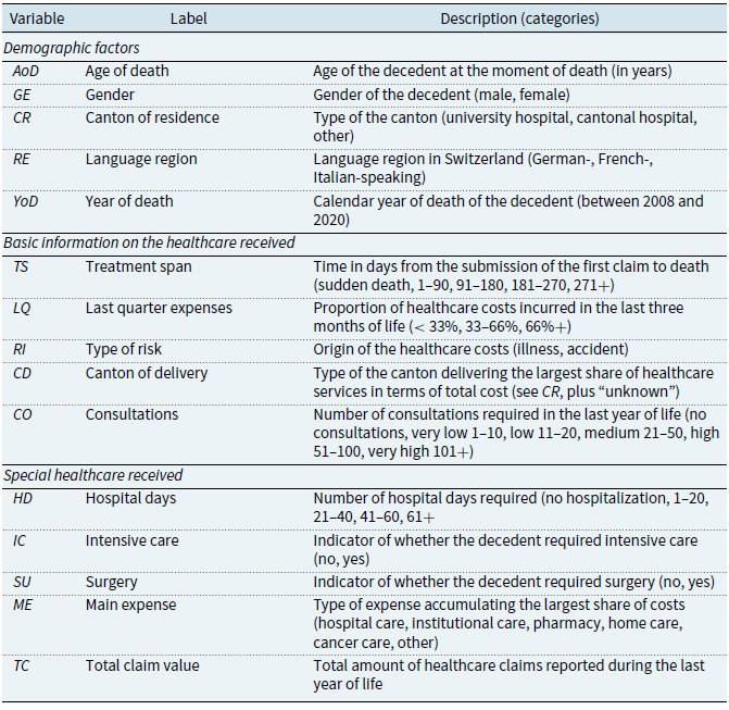
From the claims, we extract 14 potentially relevant variables to explain healthcare costs. We describe them below and give a summary in Table 1. The variables are divided into three categories: demographic factors, basic information on the healthcare received, and special healthcare received.

Table 1. Summary of the variables used in the study

Demographic factors

The dataset allows us to access primary demographic information of the individuals. First, the age of death ( $AoD$ ) is recorded as an integer variable. In the presentation of the descriptive statistics, we group the deceased into the categories 40 or less, 41–50, 51–60, 61–70, 71–80, 81–90, and 91 or older. However, we keep the variable continuous for all other analyses. The data also contain the gender ( $GE$ ) and the canton of residence ( $CR$ ) of the decedent. Given that there are 26 cantons in Switzerland, we avoid having 26 classes with relatively few observations by grouping the cantons into three categories, namely, those with a university hospital, a cantonal hospital, and neither a university nor a cantonal hospital (“other”). From the canton of residence, we group the deceased into the German-, French-, and Italian-speaking language regions ( $RE$ ). Finally, the calendar year of death is reported in $YoD$ .

Basic information on the healthcare received

The following variables relate to the deceased’s recourse to health services. Based on the dates of the submitted claims, we calculate each individual’s treatment span ( $TS$ ) as the time, in days, spent from the first claim submitted to the time of death. We group this information into the categories “sudden death” for those whose first claim coincides with the date of death, 1–90 for those who died within 90 days after submitting their first claim, and so on for the categories 91–180, 181–270, and 271+. This variable allows us to assess how many quarters a person has received healthcare attention. To complement these variables, we include the proportion of total spending incurred in the last quarter of life ( $LQ$ ), a proxy for the intensity of healthcare received in the last three months before death. While keeping $LQ$ continuous in our analyses, we group the deceased into the categories “ $\lt 33\%$ ,” “33–66%,” and “66% +” in the descriptive statistics. In addition, we code the information on whether claims were due to illness or accident in a type of risk variable ( $RI$ ). Furthermore, we record the canton of delivery ( $CD$ ) using the same categories as in $CR$ above. Since an individual may receive healthcare services in several cantons, we sum the total cost incurred in each canton and define the canton of delivery as the one where the highest costs are borne. Finally, the variable $CO$ accounts for the number of (medical) consultations the individual received. For the presentation of the descriptive statistics, we group the deceased into the categories “no consultation” for those who died without a record of consultation, “very low” (1–10 consultations), “low” (11-–20), “medium” (21–50), “high” (51–100), or “very high” (101+). However, we keep the variable continuous for all other analyses.

Special healthcare received

An interesting feature is knowing if and how long individuals required hospitalization. We estimate the number of hospital days ( $HD$ ) each deceased required. In the descriptive statistics, we use five categories: those who did not require hospitalization and those with 1–20 days, 21–40 days, 41–60 days, or more than 60 days of hospitalization. In addition, the binary variables $IC$ and $SU$ encode if individuals required intensive care or surgical services, respectively. Finally, each claim describes the health services received. With this information, we calculated each person’s expenses per category and defined a person’s main expense ( $ME$ ) by the category cumulating the highest costs. The categories include “hospital care” for hospital services, “institutional care” for care in geriatric clinics and LTC facilities, ³ “pharmacy” for drugs, “home care” for medical care and help received at home, “cancer care” for claims related to oncology and radiation therapy, and “other.” ⁴

2.2 Descriptive statistics

General observations

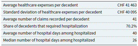
Our dataset contains the claims of $30,800$ decedents: $16,758$ males and $14,042$ females. A total of $30,615$ deaths are due to disease, and $185$ are due to accidents. As expected, a person tends to make more than one claim in the last year of life. We focus on the total cost per individual since healthcare providers have different billing policies that may affect the number of claims submitted. Basic statistics show that the average cost before death is about CHF $41,000$ during the last year of life (see Table 2). For comparison, the study developed by Panczak et al. (2017) found that the average cost of care during the last year of life in Switzerland was CHF $32,500$ . We find that in 25% of the cases, total expenses were CHF $14,986$ or less, while in 75% of the deaths, the expenses were at most CHF $53,673$ . A share of $70.2\%$ required hospitalization.

Table 2. Selected overall statistics

As shown in Fig. 1(a), the data cover deaths in all age groups from 0 to 109. However, the count peaks for decedents between 85 and 90. At these ages, we record between $800$ and $900$ deaths, for a total of $5194$ cases, or $16.9\%$ of the total. Overall, $80.5\%$ of the sample died after age 60. In Fig. 1(b), we report the average individual costs per year of death from 2008 to 2020. For this graph and all subsequent analyses, we adjusted the amounts to 2020 CHF to make the values comparable after inflation using the rates taken from the Federal Statistical Office (2022). Below, we discuss statistics along the variables and their categories (see Table 3).

Table 3. Distribution of decedents, average cost per decedent, and standard deviation

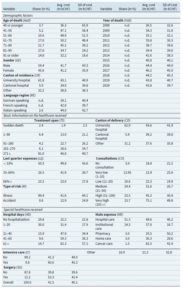
Note: “n.d.” indicates information not disclosed for confidentiality reasons. Statistics for $AoD$ , $HD$ , $LQ$ , and $TS$ are reported by category, although they are kept continuous in the modeling.

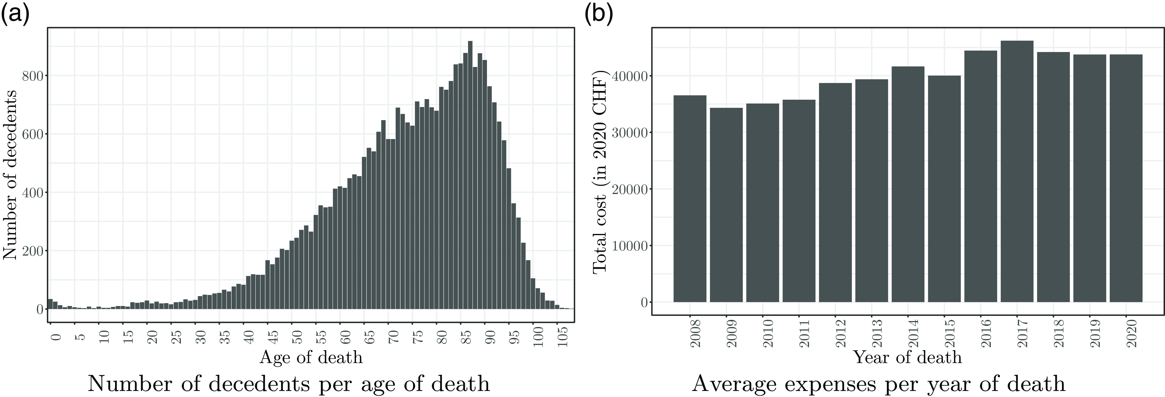
Figure 1 Distribution of the number of deaths per age and the healthcare expenses per year.

Demographic factors

The statistics along the age of death show that the average pre-death expenses tend to increase until age 60 and then decline steadily. We also observe that the average expenses of women are slightly lower than men’s (CHF $41,200$ vs. CHF $41,700$ ). Regarding the canton of residence, we find that people living in cantons with a university hospital tend to have higher EOL care costs. Language regions show differing average costs per death, with higher costs in the French- and Italian-speaking regions. This observation aligns with the conclusions of Panczak et al. (2017), who found that costs are higher in the “Latin-speaking parts of Switzerland.” Fischer et al. (2006) find that physicians’ attitudes toward EOL decisions in Switzerland may vary by language region, affecting the cost of medical care. For example, they find that physicians in the French-speaking region may be more likely to support the use of additional drugs to alleviate pain and other symptoms. Physicians in the French-speaking region were also found to be “less supportive than German-speaking doctors of the statement that doctors should comply with a patient’s request for non-treatment decisions” (Fischer et al., 2006). Both tendencies may partly justify the higher costs. Finally, the variable year of death shows no clear evolution in the cost of dying over the period analyzed.

Basic information on the healthcare received

The figures for the treatment span show that $2.4$ % of decedents died imminently, requiring healthcare for CHF $1400$ on average. In contrast, $81\%$ of individuals submitted claims during more than 270 days (9 months) before their death, confirming that most individuals in our sample required healthcare services for an extended period. The average cost for this group is CHF $46,800$ . Information on the proportion of costs incurred in the last quarter shows that half of the individuals ( $50.3\%$ ) spent less than one-third of the total costs in the last three months of life. Decedents in this group incurred an average expense of CHF $49,800$ . We observe a decreasing pattern, with a smaller proportion of decedents spending more than two-thirds of their healthcare costs in the last quarter. The latter have lower average expenses. Those who died as a result of an accident have spent much less on healthcare than those who died from illness (CHF $12,900$ vs. CHF $41,600$ ). However, as mentioned, accidental deaths represent a tiny proportion of the sample ( $0.6\%$ ). Decedents receiving most of their care in cantons with university hospitals tend to have higher average costs (CHF $43,600$ ) compared to others (CHF $39,200$ for cantons with a cantonal hospital, CHF $37,600$ for others). We observe that most decedents ( $62.9\%$ ) received most of their treatment in cantons with university hospitals. This aligns with the proportion of people living in such cantons ( $61.8\%$ ). A share of $3.9\%$ died without any record of medical consultations. These individuals spent an average of CHF $18,900$ , which is significantly less than all other groups. We also find that healthcare costs increase with the number of consultations. For example, deceased who had more than 100 consultations accumulated average costs of CHF $75,100$ . In contrast, those with 1–10 consultations spent on average CHF $15,900$ .

Special healthcare received

As reported in Table 3, $29.8\%$ of the individuals in our data did not require hospitalization, and their average cost is significantly lower. We find confirmation that costs increase with the length of hospitalization. In addition, we document that only a small proportion required intensive care services ( $0.8\%$ ) and that those who did, not surprisingly, had much higher costs (CHF $60,600$ compared to CHF $41,300$ ). In addition, $12.2\%$ of the deceased required surgical services, also yielding a much higher average cost (CHF $53,300$ ). Finally, the most recurrent expenses are hospital care ( $51.3\%$ ) and institutional care ( $24.3\%$ ). Those whose main expense was hospital care had an average cost of CHF $49,600$ . In contrast, those in the institutional care category cost CHF $37,000$ . The most expensive cases relate to cancer treatments, with decedents having claimed CHF $83,300$ (see also, e.g., Polder et al., 2006).

2.3 Additional statistics

Types of expenses by age groups

In Fig. 2(a), we show the variation of the main expense category along the age classes. We observe that hospital care cost is the main expense for most of those who die at younger ages. While 49.1% of those dying at age 40 or younger have hospital care as their main expense, only 20.8% of those dying in their 90s do. Dying younger also implies the need for healthcare services beyond cancer treatment or pharmaceutical services and home and institutional care that are primarily irrelevant. This results in a large proportion being classified in “other.” The latter main expense accounts for 46.5% of deaths at ages below 40 and 29.5% of deaths between 41 and 50. The graph also confirms that institutional care in the last year of life is critical for those dying at older ages. More than half ( $63.9\%$ ) of those dying at age 91 and older had most of their spending on institutional care. Similarly, those dying between the ages of 81 and 90 also made significant use of institutional care services ( $39.7\%$ ). Thus, it can be expected that the role of institutional care will become even more critical in the future as the chances of surviving beyond the age of 80 improve.

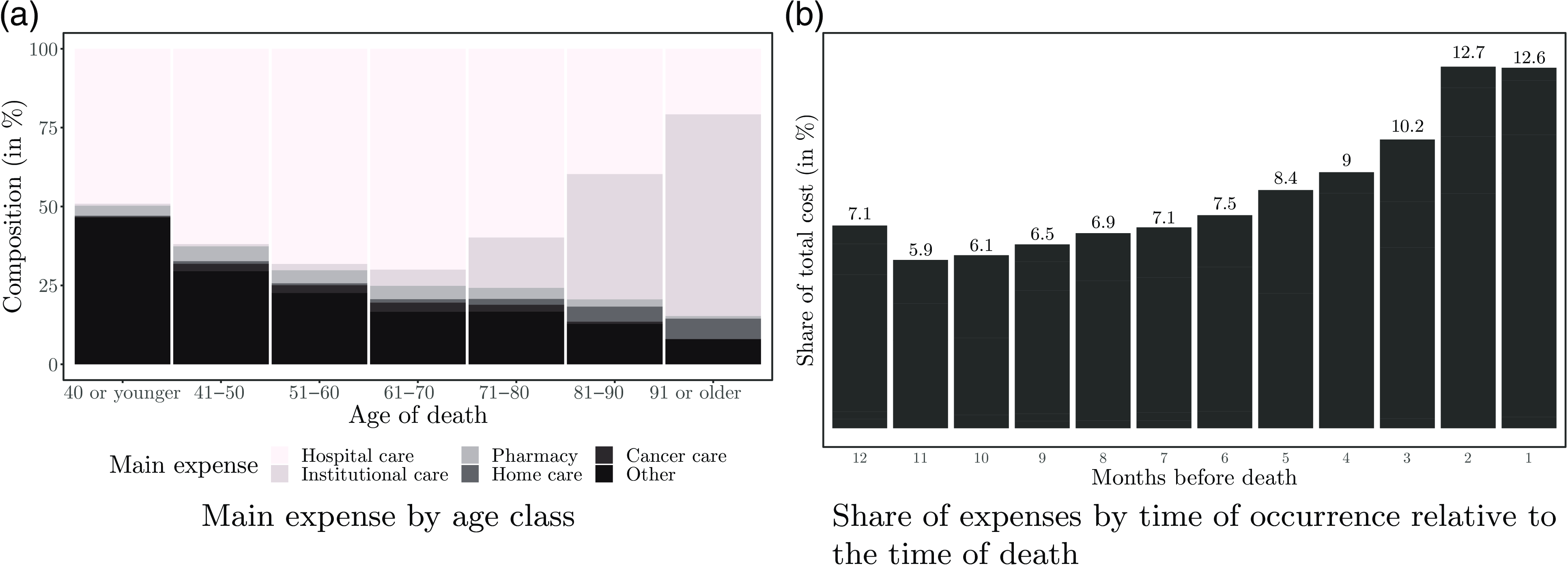
Figure 2 Types of expenses by age class and distribution by proximity to death.

Influence of the proximity to death

In the introduction in Section 1, we pointed out that several authors found an association between proximity to death and healthcare costs. To explore this effect, we compute the proportion of total healthcare spending per month when considering the time of treatment relative to the time of death. The results are shown in Fig. 2(b). We find a clear pattern confirming that healthcare costs increase as death approaches. The figure indicates that treatments required 7–12 months before death account each month for about 6–7% of total costs. In contrast, treatments received in the last two months of life account for about $13\%$ each month.

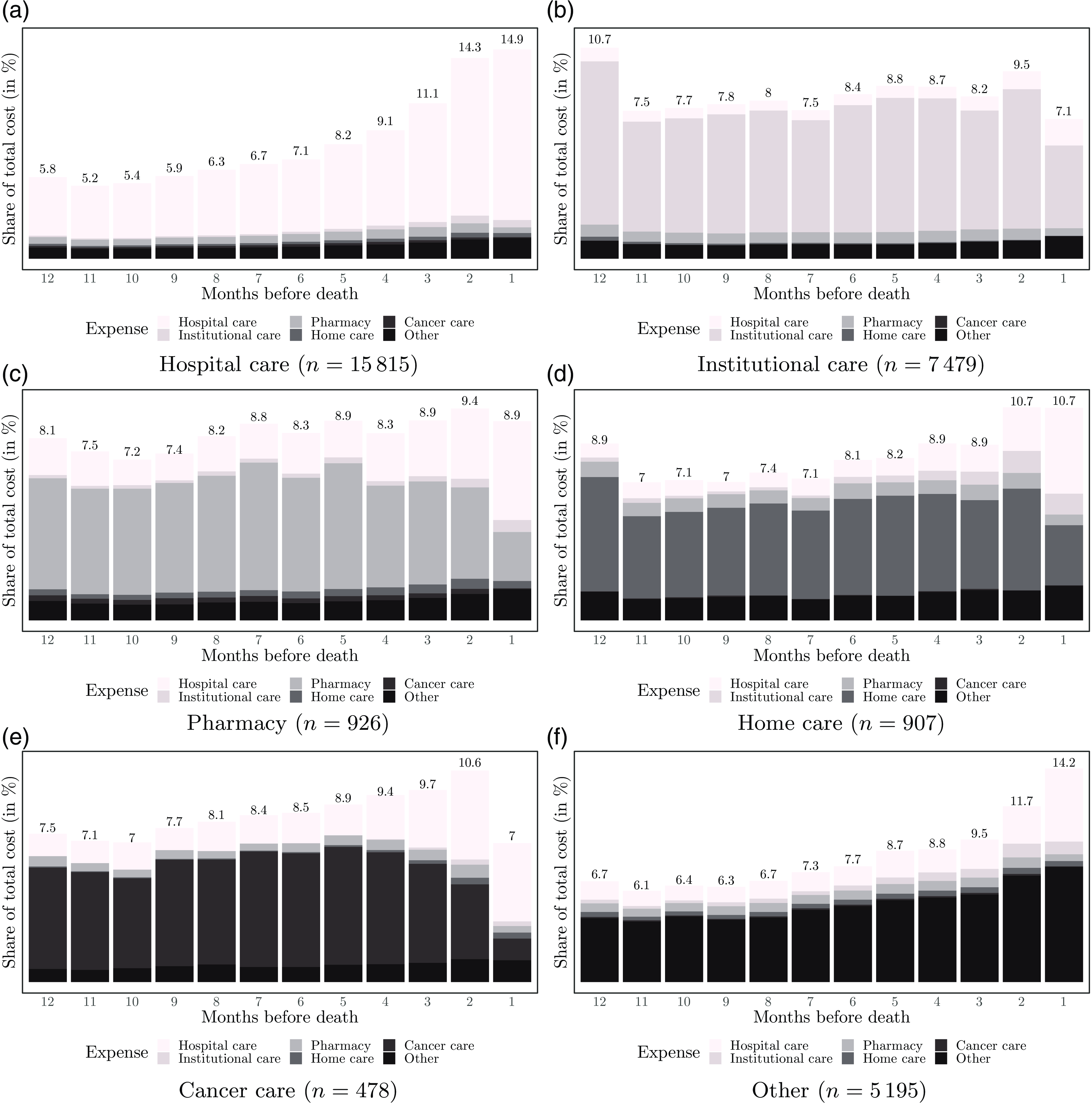
Figure 3 Breakdown of expenses according to their occurrence relative to the time of death and the decedents’ main expense.

Evolution of expense patterns

To enrich our analysis, we explore the evolution of patterns by grouping individuals by their main expense (see Fig. 3). For example, in Fig. 3(a), we observe that the spending of those with hospital care as their main expense is similar to the overall pattern shown in Fig. 2(b). The same holds for the group of decedents in the main expense category “other,” except for the more pronounced cost increase observed in the last two months of life, as shown in Fig. 3(f). In contrast, those requiring mostly institutional care show a stable spending pattern over the 12 months; see Fig. 3(b). For these decedents, we document a decrease in costs in the last month of life, which may be related to a decrease in services in the last days before death. The stability of costs in the institutional care group contrasts with those who have home care as their main expense. As shown in Fig. 3(d), expenses are relatively stable until the last months before death. Before death, expenses gradually increase and peak in the last two months. This increase can be explained by increased hospital costs due to transfers from home to hospital. This supports previous findings suggesting that most dying people spend more time in hospitals than desired, even when their preference is to be cared for at home (Cohen et al., 2007; Luta et al., 2020). We do not observe this transition to hospital to the same extent in the group that mostly received institutional care.

Another interesting feature can be observed in Fig. 3(e), focusing on those with cancer treatment as the main expense. For these decedents, we document a steady expenditure increase as death approaches. While the large share of cancer-related expenses remains stable until the last two months of life, hospital care expenses add to it. However, in the last month of life, we find a sharp decrease in spending related to the reduction in cancer treatment. This could signal a transition to less aggressive EOL care, suggesting that physicians stop more invasive and drug treatments in the weeks or days before the patient’s death. This could be intentional, as aggressive care for terminal cancer patients is usually associated with “poor outcomes such as prolonged pain and overall dissatisfaction with care” (Henson et al., 2016). Finally, although the PDQ Supportive and Palliative Care Editorial Board of the National Cancer Institute (2022) indicates that cancer patients may prefer to die at home, claiming that they feel “better prepared for death” at home than in a hospital or intensive care unit, we observe that patients in Switzerland are characterized by higher hospital expenses in the last weeks of life. In addition, it is worth noting that hospital expenses increase substantially with proximity to death.

3. Model framework

For each decedent, we consider the main variable of interest $y=TC$ , that is, the total value of healthcare claims, and its characteristics, which are described by a selection $\mathbf{v}$ among the 14 variables from the set of covariates $\mathcal{V}$ presented in Table 1. We assume that $\mathcal{V} \subset \mathcal{W}$ , where $\mathcal{W}$ is a higher dimensional space of variables that explains an individual’s healthcare spending. Thus, we aim to find a model $\hat {M}$ that approximates the true and unknown model $M$ and explains the relationship between the covariates $\mathcal{W}$ and the response $y$ such that $ \hat {M}\,{:}\, \mathcal{W} \xrightarrow \ y$ .

We train candidates for the model $\hat {M}$ using statistical techniques including machine learning. We fit RFs and GBMs as alternatives to generalized linear models (GLMs). These two methods are chosen as alternatives to more classical models because there are tools for interpreting their results, which can help with our primary objective of understanding the influence of different factors on the cost of dying. By training these different models and evaluating their performance, we aim to find the model that best explains the relationship between medical expenditures and the covariates without assuming ex ante that any particular model will perform better. Since the three approaches have different characteristics that may make them (un)suitable to explain a particular relationship, we propose to try several of them but ultimately will keep only the one that is considered “the best” for our analysis. The models’ performance is evaluated with the $R$ -squared and the root mean squared error ( $RMSE$ ) measures. These are two widely used and familiar measures for assessing the performance of models where the outcome variable is a number, as in our case (see, e.g., Kuhn & Johnson, 2013). Although our main objective is not to make predictions, we believe that analyzing the performance of models using these indicators helps to corroborate the credibility of the effects suggested by the different methods and the conclusions drawn from them.

Generalized linear models

GLMs are typically used as the first instance when fitting candidate models for $\hat {M}$ . We start by considering all variables in $\mathcal{V}$ and reducing the number of covariates used for model training. Therefore, we perform a stepwise variable selection procedure with the objective to minimize Akaike’s information criterion (AIC). ⁵ We implement this procedure using the caretpackage in R. The best model includes 12 from the initial 14 variables.

Random forests

RF techniques emerged in the early 2000s and are based on decision trees. Although decision trees are beneficial because of their interpretability, using only one tree can lead to a decrease in accuracy, overfitting, and loss of information problems. RFMs improve this by “exploiting the natural variability of trees, introducing some randomness in the selection of both the individuals and variables” (Genuer & Poggi, 2020). Taking $T$ as the number of trees to grow, Breiman (2001) defines a random forest as a collection of trees ( $\hat {h}(\Theta _1)$ , $\hat {h}(\Theta _2)$ , …, $\hat {h}(\Theta _T)$ ), with { $\Theta _k$ } independent and identically distributed random vectors, where each $\hat {h}(\Theta _k)$ gives an estimate ( $k=1,2,\ldots, T$ ). Different models of the form $\hat {h}(\Theta _k)$ are aggregated into the random forest, $\hat {h}_{\textrm { RF}}(x)$ , which gives the final estimate based on the average result of all trees.

Gradient boosting machines

Gradient boosting provides a way to add new models to a sequence, where each iteration creates a new learner that is “trained with respect to the error of the whole ensemble learned so far” (Natekin & Knoll, 2013). In this approach, each new tree is designed to provide a more accurate approximation of the variable of interest. The technique is well known for outperforming other models and is considered one of the best choices when dealing with multiple data types (Chollet et al., 2022). In addition, as is the case for tree-based models, RFs and GBMs offer documented advantages such as a superior ability to handle multicollinearity, missing values, and high dimensionality (Afanador et al., 2016; Chowdhury et al., 2022; Song et al., 2020; Vaulet et al., 2022). When dealing with two correlated variables, tree-based models would split by choosing one instead of both. As they are an ensemble method, built with multiple individual trees, an analysis with enough weak learners (individual trees) should offer “a high level of assurance that the relationship between collinear variables will be adequately captured via averaging” (Afanador et al., 2016).

Model selection and implementation

In a preliminary correlation analysis, ⁶ we found that the features associated with the canton of delivery ( $CD$ ) and of residence ( $CR$ ) are highly correlated (with correlation coefficients up to $0.90$ among the categories). This may follow because most individuals receive treatment in the canton where they reside. For this reason, we omit the canton of residence variable from the model. We also observe a strong correlation ( $0.70$ ) between being from the Italian region and being treated in a cantonal hospital. However, we observe that only a very small proportion of individuals in our data come from the Italian region, and the most prominent French and German regions do not strongly correlate with the type of canton of delivery. Another important correlation, but lower in magnitude ( $-0.47$ ), is observed between the variables relating to the treatment span ( $TS$ ) and the proportion of healthcare received in the last three months before death ( $LQ$ ). Therefore, we have decided to retain all these variables in our model and perform a generalized variance inflation factor analysis later to determine if multicollinearity issues may arise. ⁷ We find that multicollinearity issues should not be expected while keeping the remaining variables. As previously mentioned, tree-based methods are known to be less susceptible to multicollinearity problems. Therefore, it is pretty unlikely that a tree-based model will be affected by multicollinearity if we have evidence that multicollinearity should not be an issue in a GLM framework.

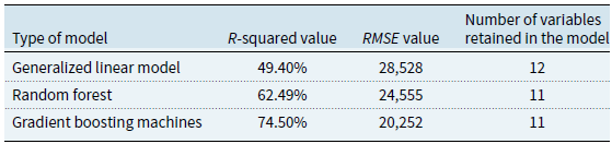
We chose the GBM model as the reference for our analysis. Indeed, as seen in Table 4, this model maximizes the $R$ -squared value and minimizes the $RMSE$ in our dataset. These are both characteristics of a preferred model. In addition to performing better in terms of $R$ -squared and $RMSE$ , the GBM provides a slightly more parsimonious model when compared to the GLM methodology (see Table 4). Our choice allows us to exploit the advantages previously mentioned. As this is the classical approach when using categorical variables to train a GBM, we have introduced categorical variables using their dummy version through one-hot encoding. As we will report in Section 4.1, our final model is trained using 15 features stemming from 11 explanatory variables and their dummified versions.

Table 4. Summary of the model performance

As stated by Friedman (2001), the goal is to use a training sample to obtain the estimate of $\hat {M}$ such that the expected value of a given loss function $L(y, M)$ is minimized. Formally, we have

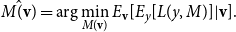\begin{equation*} \hat {M(\mathbf{v})}=\textrm {arg}\min _{M(\mathbf{v})}E_{\mathbf{v}}[E_y[L(y,M)]|\mathbf{v}] . \end{equation*}

In our implementation, we use the package XGBoostand consider as loss function the square loss, a choice that is commonly used in practice (Natekin & Knoll, 2013). This means that the algorithm will perform a residual fit at each iteration. The desired number of iterations must be determined in the modeling process. We estimate the optimal number of iterations by stopping the algorithm early if the error does not improve after ten consecutive rounds. We find that 24 iterations are sufficient using this method, so we keep this as our parameter.

To ensure the interpretability of our results, we use both a variable importance analysis and the calculation of PD coefficients. The variable importance analysis indicates how relevant a feature is in explaining healthcare expenses. This is done by estimating “the fractional contribution of each feature to the model based on the total gain of this feature’s splits” (Chen & Guestrin, 2016). This fractional contribution is typically referred to as the sum gain. In addition, PD coefficients are estimated using the PDPpackage in R. These coefficients show the marginal effect of a variable (or a pair of variables) on the results of a model. Since PD coefficients can be difficult to interpret in the case of continuous variables (where there may be hundreds of points), we focus on the main trend they represent. To achieve this, we fit third-degree polynomials to approximate the coefficients found.

4. Results and discussion

In the following, we present the results of the analysis. First, we report our findings on the importance of the variables in Section 4.1. We then quantify the effects using the PD coefficients in Section 4.2. Finally, the main results are discussed in Section 4.3.

4.1 Variable importance

Figure 4 illustrates the variable importance results. The number of consultations and hospital days are Switzerland’s most important drivers of EOL healthcare expenses. This is consistent with recent findings of Luta et al. (2020) that “the main driver of healthcare intensity and costs is inpatient hospital care.” Another essential factor is the age of the deceased. Among the five most relevant characteristics, we also find the proportion of expenses in the last quarter and the treatment span. Other relevant features are the type of the deceased’s main expense and whether the deceased lived in the French-speaking part of Switzerland. Finally, whether decedents received most of their care in a canton with a university hospital, their gender, whether they died in 2017, and their need for surgical services play a role. These are the characteristics included in our model.

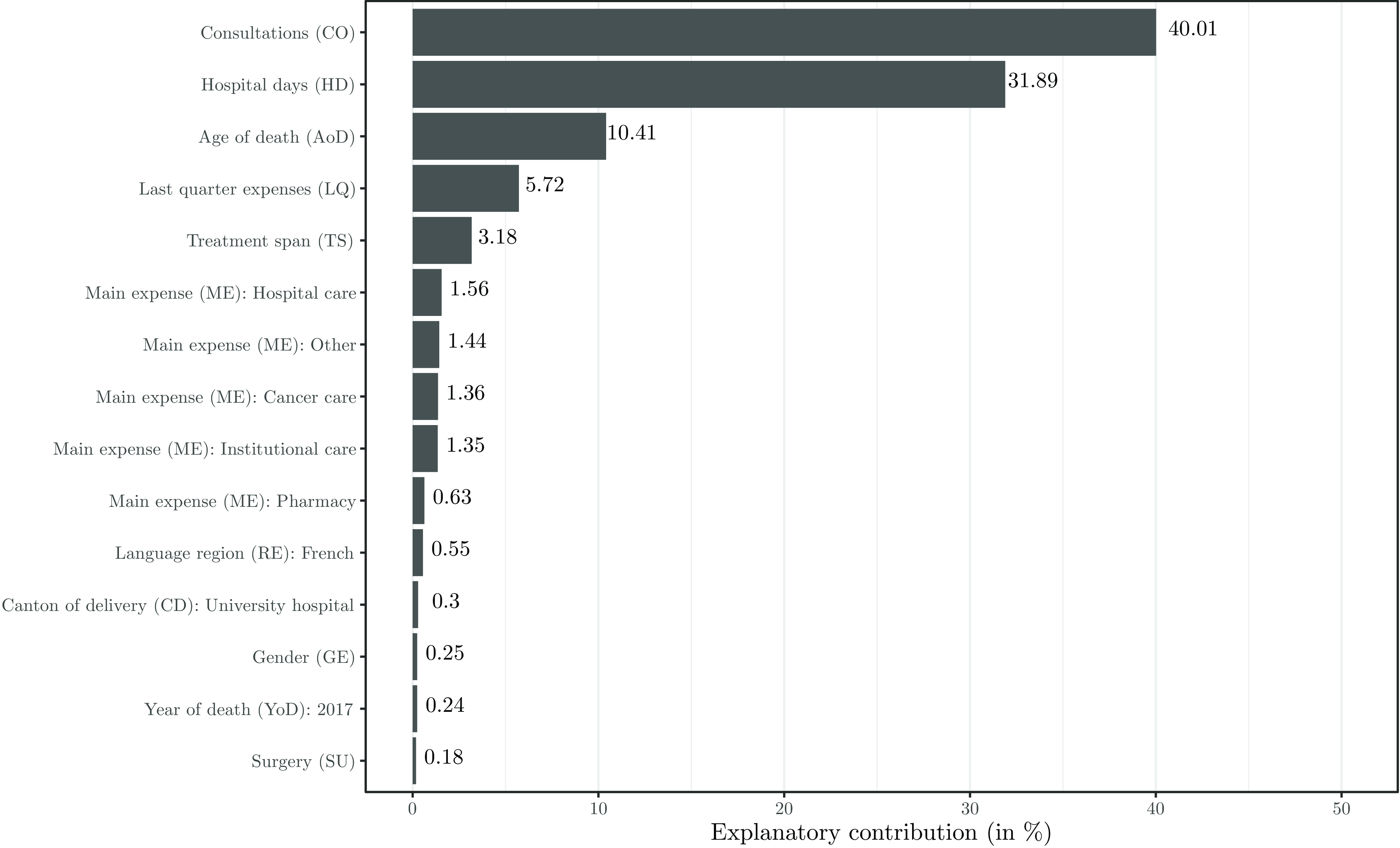
Figure 4 Explanatory contribution of the 15 features retained in the GBM model.

4.2 Quantification of effects

In the graphs of Figs. 5 and 6, we show the effect of the number of consultations and hospital days, the age of death, the share of last quarter expenses, and the treatment span through the associated value in CHF of the PD coefficients. The average expected cost of dying estimated by the model is CHF $41,444$ , which is very close to the average of CHF $41,463$ reported in the statistics (see Table 2). We indicated the estimated average by a dashed horizontal line. For each value of the variable of interest, we show the cost estimate (dots), and the solid curve represents the fitted cubic polynomial. The PD coefficients show a pattern rather well explained by the polynomial with the $R$ -squared measure of the fit tending to values above 90%.

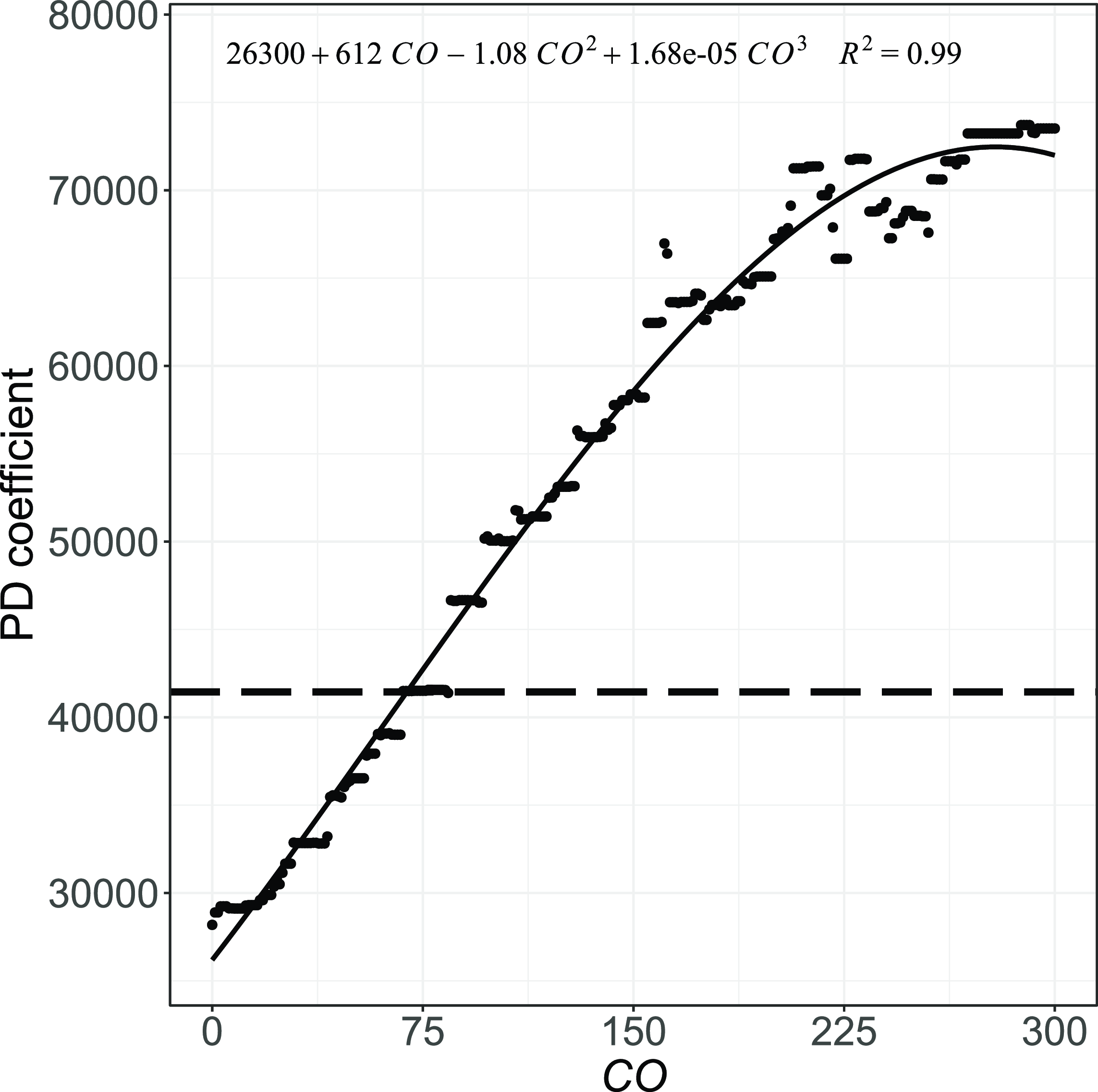
Figure 5 Estimated effect (PD coefficient) of the number of medical consultations.

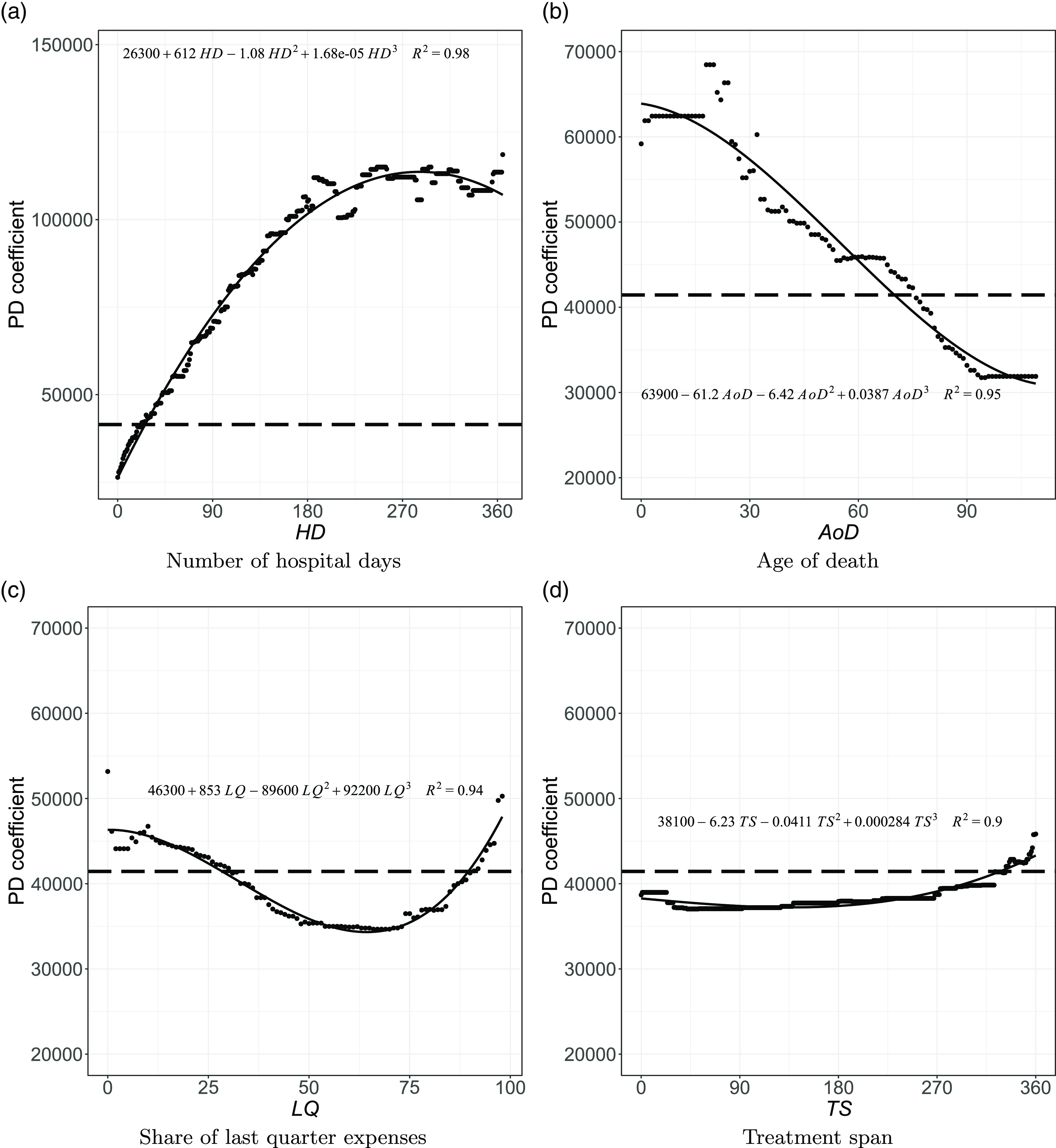
Figure 6 Estimated effects (PD coefficients) on the expected cost for the other continuous variables.

Note: The horizontal dashed line indicates the average expected cost (CHF 41,444), the dots represent the expected cost along the covariates, and the solid curve represents the fitted polynomial.

The overall trend of the PD coefficient analysis indicates that costs tend to increase with the number of consultations and hospital days, as shown in Figs. 5 and 6(a). The average expected cost would be CHF $28,186$ if all individuals had died without requiring any consultation, other things being equal. This estimate increases to CHF $29,114$ had they required 10 consultations in their last year of life, and CHF $32,844$ in the case of 30 consultations. While more frequent consultations are associated with higher direct costs, they also typically lead to additional prescriptions, increasing healthcare spending. Recurrent consultations are often associated with persistent symptoms or conditions that require regular monitoring and may signal more complex health profiles. In the case of hospital days required, the cost would be $26,366$ if all individuals were assumed not to require hospitalization. On the other hand, if all decedents had required about 60 days (two months) of hospitalization in their last year of life, the expected cost would increase to over CHF $55,000$ . Had it been 90 days (3 months), this amount would have reached CHF $68,934$ . The increasing costs with the number of hospital days reflect the impact of hospitalization on healthcare spending.

Moreover, the cost of dying tends to decrease for older decedents, as shown in Fig. 6(b). For example, the expected healthcare expenditure would be CHF $59,456$ if all decedents were 25 years old, ceteris paribus. In contrast, this cost would be $44,072$ if they were assumed to die at age 70. Overall, decedents aged 75 or younger have higher-than-average expected claims. This observation is consistent with previous findings. For example, Scitovsky (1994) found that “while [Medicare] payments for survivors increased with age, those for decedents decreased.” The results by Werblow et al. (2007) point to “high costs of dying that decrease in old age.” Based on their findings, they state that “deaths may well be more costly both in absolute and relative terms at young than at old age.” Jecker and Schneiderman (1994) analyze the psychological perceptions of death. They argue that older people tend to anticipate death as an imminent event, while younger people tend to be more resistant. As a result, “a medical team may be more inclined to press for aggressive interventions, despite low odds of success, when the dying one is a child, rather than someone age 80,” they explain. By this logic, younger patients may be subjected to more intensive (and expensive) treatments to save their lives, thereby increasing the costs. In addition to this psychological explanation, this effect may result from an implicit financial calculation, where some are more willing to pay to save a life that may result in a higher societal return (Schelling, 1968; Zweifel et al., 1999). Examples of this come from the COVID-19 pandemic. As an illustration, Ghamari et al. (2022) asked medical specialists about their priorities in allocating ventilators. While pregnant women were considered the highest priority, followed by mothers with children under five, $45.7\%$ of the specialists agreed that patients over 80 would receive lower priority.

As seen in Fig. 6(c), a concentration of less than $30\%$ of expenses in the last quarter is consistently expected to lead to higher-than-average healthcare spending. Indeed, if a decedent accumulated less than $30\%$ in last quarter expenses, they most probably received care for longer (and more frequently) throughout the year, resulting in overall higher expenses. Regarding the treatment span, Fig. 6(d) confirms that the earlier the decedent started making claims, the higher the healthcare costs, corroborating that requiring care for an extended period is associated with higher costs. This is reasonable if claims are recurrent, which is plausible given we only consider the last year of life. The PD coefficients show the pattern of a staircase up to 300 days (10 months) of treatment. Healthcare costs are expected to be substantially lower when individuals die within 100 days from the first claim. If all individuals had died during this period, all else being equal, the expected cost would have ranged between CHF $37,000$ and CHF $39,000$ .

The PD coefficients from the categorical variables are reported in Table 5. Since these variables are introduced as dummy variables, the PD coefficients show the expected cost if all individuals are assumed to have the characteristic (column “Yes”) compared to when they do not (column “No”). Among the variables depicted in Fig. 4, our results confirm that cancer care is a significant cost driver (PD of CHF $62,923$ ). This is consistent with the results presented by Panczak et al. (2017). In contrast, assuming that all decedents received institutional care (CHF $43,492$ ) or hospital care (CHF $41,867$ ) results in expenses close to the average expected cost of CHF $41,444$ .

Table 5. Estimated effects (PD coefficients) on the expected cost for the categorical variables

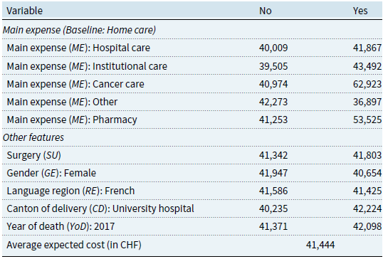
The need for surgery is another driver of EOL healthcare costs. If all decedents had required surgery, the average healthcare expenses would be CHF $41,803$ as opposed to CHF $41,342$ . Indeed, surgeries are expensive procedures that often involve additional risks and complications, triggering further healthcare services and expenses (Institute for Healthcare Policy & Innovation, 2019). Men are expected to spend more than women (PDs of CHF $41,947$ vs. CHF $40,654$ ). In addition, residence in the French-speaking part of Switzerland (PD of CHF $41,586$ ) leads to slightly higher costs than in the rest of the country (CHF $41,425$ ). Our data suggest that the EOL is pricier in cantons with a university hospital (CHF $42,224$ vs. $40,235$ ). University hospitals in Switzerland are known for the quality of their services. They are typically ranked among the best medical centers in the country (see, e.g., Cybermetrics Lab, 2022; Newsweek, 2022). This may justify the higher costs in these cantons that provide access to the best treatments. Finally, the model suggests that dying in 2017 leads to a higher cost of dying ( $42,098$ vs. $41,371$ ). This is in line with the results displayed in the descriptive statistics section (see Table 3), where this year has the highest average cost. However, as seen in the descriptive statistics, there is no clear cost trend over time. This is confirmed by the fact that only this year is included in the model and by its lower importance compared to other features.

4.3 Discussion

Drivers for longer hospital stays

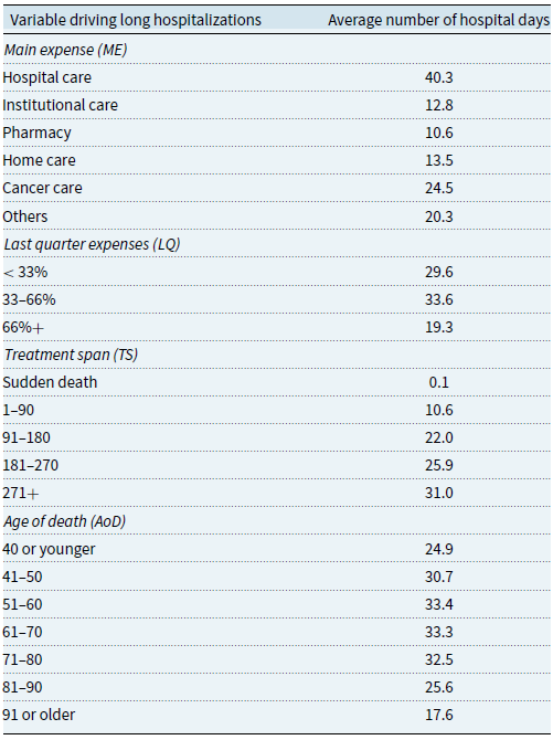
A recurring element is the cost of hospital care in the last year of life. Indeed, hospitalization leads to significantly higher costs, as we have shown. To gain further insight, we perform additional analyses to understand the main characteristics of those hospitalized the longest. ⁸ Table 6 presents the average number of hospital days and the variables found to be the most relevant drivers. More extended hospital stays can be explained mainly by characteristics related to the individual’s main expense ( $ME$ ), the proportion of healthcare costs incurred in the last three months of life ( $LQ$ ), the individual’s treatment span ( $TS$ ), and the patient’s age at death ( $AoD$ ). Individuals with long hospitalizations can be more likely to have hospital care as their main expenditure, so individuals in this category have, on average, more than 40 days of hospitalization in the last year of their lives. A more informative result comes from the institutional care category, associated with less than 13 days of hospitalization. Their average level of hospitalization is lower than that of individuals whose main expense is home care, but the latter are much less numerous, as shown in Table 3. The results in Fig. 3(b) already suggested that those in institutional care had the smallest share of hospital spending as death approaches. Similarly, Füglister-Dousse and Pellegrini (2019) find that individuals in institutional care have a lower risk of repeating hospitalizations in the last months of life. Our findings seem to confirm these conclusions. In addition, we observe that those who use between $33\%$ and $66\%$ of their total spending in the last quarter are hospitalized the most, with an average of 33.6 days. We also observe a clear pattern where the longer the treatment span, the greater the average number of hospital days. This confirms that higher hospitalization rates appear to be associated with patients who undergo longer treatments, requiring health services for most of the year. Longer treatments seem to be intensified in the last quarter of life, most likely in the form of hospitalizations, which justifies their relatively high level of expenditure in the last three months. Table 6 also shows that individuals who die between the ages of 51 and 70 tend to be hospitalized for longer, with deaths after 80 being associated with substantially fewer hospitalizations. This is in line with our previous results on the role of institutional care. Overall, individuals who die before reaching age 80 seem to go through hospital stays that add up to at least a month on average. As these individuals may be considered quite young to die in the current demographic context, these longer hospitalizations are likely to be an attempt to save the person’s life.

Table 6. Statistics on the average number of hospital days along relevant variables

On the role of hospitalization substitutes

If new policies to control healthcare spending are developed, hospitalization strategies and potential substitutes must be rethought. In this sense, creating the right network of services to encourage more institutional or home care during the last year of life may be critical to both reducing hospital costs and allowing people to spend more time with their loved ones. In the United Kingdom, for example, policymakers attach great importance to the place of death when developing EOL care policies to decrease the number of inappropriate hospital admissions (Hoare et al., 2019; Morris et al., 2013). Researchers, however, have found multiple factors threatening the emergence of places such as community-based centers or even the decedent’s home as an appropriate place to die. According to Morris et al. (2013), emotions, beliefs, and habits play a key role when individuals have a choice about their place of death, which may cause patients to change their preferences for hospital care as their condition worsens. The availability of caregivers may be a challenge even when sick individuals prefer to die at home. Hoare et al. (2019) state that many find it difficult to care for a loved one who is dying and whose condition is deteriorating. They state that “naive carer expectations of the dying process were thought to hinder the likelihood of death at home, as unfamiliar but typical symptoms of EOL care were reported to lead carers to seek reassurance and care.” In Switzerland, a study by Eggli et al. (2022) confirms that lack of security at home is a frequent cause of unnecessary hospitalizations. This may help explain why hospital expenses increase so abruptly in the last two months for those who had at-home care as the main expense (see Fig. 3d). In this sense, many of those individuals could have lacked the tools to be cared for at home during that period. Developing a policy to incentivize more institutional, community, or home-based care is likely to require significant investments on additional facilities and staff, as well as better training or support for family members caring for a loved one.

Current and future role of long-term care is key

It could be expected that more people will die in nursing homes in the future. A significant proportion (24.3%) of our sample has institutional care as their main expense. Hence, it is essential to consider the future capacity to care for an aging population in these facilities. In Switzerland, demand will likely increase as the number of people aged 80 and over is expected to reach over one million in the next 30 years (Federal Statistical Office, 2018). In addition, a significant proportion of them are expected to require LTC services (Fuino & Wagner, 2018). This combination of factors could generate a sharp increase in the number of people dying in institutions, which may be particularly critical in terms of financing, given the lack of interest in LTC insurance purchase (Fuino et al., 2022; Ugarte Montero & Wagner, 2023). Options for meeting the growing need to cover EOL care costs must be carefully analyzed. As Bone et al. (2018) note, “knowledge of where people are likely to die is an important indicator of where pressures in the health system may occur in future years.”

Disease patterns and personal choices

It is crucial to understand how diseases evolve and how the patterns of healthcare costs are affected. For example, Thomas (2021) states that the proportion of the population living with more than one chronic condition is increasing. This trend toward multimorbidity increases the need for individualized treatment solutions. While EOL care has historically been organized around specialist care in acute settings, the evolution of chronic conditions may present a challenge. In addition, the Swiss Re Institute (2023) states that the aging of societies will come with more neurodegenerative diseases as a cause of death. In this context, it is crucial to reflect on the role of palliative care as part of the healthcare offering in the last months of life. Rather than prolonging life, palliative care will focus on providing quality of life in the last days (Kelley & Morrison, 2015). For example, Sallnow et al. (2022) address that very often, dying people receive excessive treatments during their last days. These treatments oftentimes neglect the role of family and friends. This can result in “increased suffering, and consume resources that could otherwise be used to meet other needs.” Part of this reflection should address how much control dying people have to avoid treatments that may increase suffering and costs in vain. It may also be essential to understand their choices regarding the place of dying and to establish mechanisms for respecting those choices whenever possible.

Limitations of our study

We acknowledge that an important limitation of our study is the lack of information on the diagnosis and the detailed cause of death of the patients. This limitation arises from the fact that health insurance companies in Switzerland only have limited information on the specific conditions that trigger the claims. Adding information on the type of health service received, which is encoded by the insurance company and which we describe in the variable “main expense,” is an attempt to compensate for this. We believe this approach still provides interesting insights. Indeed, analyses not including the cause of death are not uncommon in the literature (see, e.g., Duncan et al., 2019; Felder et al., 2000).

Our study covers a multiyear period ending in 2020, which corresponds to the beginning of the COVID-19 pandemic. We confirm that the deaths recorded in our dataset are indeed more numerous for 2020 compared to other years. For example, the average annual increase in the number of deaths for the years 2008–2019 was 11.1%. In contrast, we observed an annual increase of 19.2% in deaths in 2020 compared to 2019. Increases in the number of deaths can be attributed to elements such as changes in the size of the insurance company’s portfolio (number of people exposed to the risk of death), the aging of policyholders, and, of course, the COVID-19 pandemic in 2020. However, the aforementioned lack of information on the cause of death or diagnosis makes it difficult to quantify the impact of the pandemic. Since our analysis period is long (13 years), this should not greatly affect the generalizability of our results. The interested reader will find specific information on the impact of the COVID-19 pandemic on mortality in Switzerland in the report of the Federal Statistical Office (2023).

5. Conclusion

A recurrent need for healthcare services in hospitals or institutions likely marks the last year of life. We show that a number of hospital days and consultations are critical drivers of EOL costs. In addition, the age at death plays an important role in the total amount of expenditures, as claims costs decrease with increasing age. While younger people are likely to receive more hospital care and life-saving treatments, older people’s costs have important institutional and home care components. The cost of dying varies with age because of the different care types provided. Moreover, we observe that most individuals live with healthcare for a longer time before they die, with the majority receiving care for at least nine months before their death.

Our findings can be helpful to insurers and governmental agencies alike. On the one hand, insurers can better understand the claim amounts and plan accordingly. They also gain insight into the factors that influence the expected costs and compare them to the actual costs of their portfolios. Governmental agencies, on the other hand, can learn about the current cost components in the year before death. This allows them to better quantify and project the spending on different healthcare services, which ultimately helps define measures and policies to improve patients’ life quality at the EOL. This knowledge can also stimulate debate about how prepared the country is to provide health services in the future. For example, it is essential to consider the capacity to meet the growing demand for institutional care. Trends in the age of the deceased and the current aging of the population indicate that certain types of healthcare services will be increasingly important. Although our study is based on Swiss health insurance data, we believe that some of our findings generally apply to developed countries facing similar trends in healthcare services in the context of an aging population.