Seismic exploration of the sea floor using fin whale songs and seismic airguns in the Bransfield Strait, Antarctica

Abstract

The use of seismic airguns has an environmental impact that is especially intense in relation to marine mammals. As a result, new techniques are being explored to replace or complement this tool. In this study, we test our ability to obtain seismic information about the shallow seafloor structure using fin whale songs as an alternative seismic source. We analyse data collected by ocean-bottom seismometers deployed around Orca volcano in the Bransfield Strait, Antarctica, in 2019. We detected fin whale calls and designed an algorithm to calculate their locations and origin times. We used a relative approach to reduce location uncertainty based on the similarity of waveforms between consecutive calls. We were able to calculate the trajectory of a fin whale that crossed over Orca volcano. Strikingly, the whale path coincided partially with a multi-channel seismic profile carried out with airgun shots. This coincidence allowed us to investigate the performance of the whale calls as seismic sources, comparing them to the almost co-located airgun profile. We constructed receiver gathers using both whale calls and airgun shots. The main features of the whale call sections are consistent with the results obtained using the airgun source. We conclude that although this method has some drawbacks, such as the unpredictable behaviour of whales and the smaller power and lower resolution capabilities of the whale calls compared to the airgun surveys, it is still a feasible alternative as a complement for active-source seismic studies in the marine environment.

Introduction

Seismology involves the study of the propagation of seismic waves generated by mechanical disturbances, including earthquakes, to investigate the internal structure of the Earth. Beyond natural seismic events, artificial sources such as hammer blows or explosions, and even the ubiquitous ambient seismic noise, can also provide valuable information within this area of study. In the context of shallow geophysical prospecting, seismic exploration using artificial sources is a non-invasive method for exploring subsurface structures. Such techniques include seismic reflection and refraction, and they complement other methods such as gravimetric, magnetic or electrical resistivity prospecting.

One common application of seismic exploration is within the hydrocarbon industry (Landrø et al. 2017). In this context, active-source marine surveys are performed using seismic airguns based on compressed-air shots that produce high-intensity acoustic pulses (over 200 dB). These signals travel through water and penetrate up to several kilometres below the sea floor (Gisiner 2016), interacting with the discontinuities of the velocity structure. The generated wavefield is then recorded either by a streamer for reflection studies or by ocean-bottom seismometers (OBSs) for refraction analyses (Dobrin & Savit 1988, van Opzeeland et al. 2014). However, airguns have recently been criticized for their environmental impact. In particular, acoustic pollution (Rodrigo Saura 2009) affects marine fauna such as cetaceans, causing behavioural changes (Castellote et al. 2012, Dunlop et al. 2020), communication disruptions (McCauley et al. 2000) and even physical harm in the worst scenarios (Weilgart 2014).

To mitigate these effects, alternative sources with smaller environmental impacts are being proposed. An example is the marine Vibroseis (Ogden 2014, Weilgart 2016), which generates signals that are longer but less intense than conventional airgun shots. Biological sources such as whale songs could also be potential and feasible alternatives. Recently, Kuna & Nábělek (2021) recorded signals of fin whale vocalizations with an OBS network deployed during a study of the Blanco Fault Zone in the North Pacific. They were able to create several seismic sections and characterize the sea floor in the area down to almost 6 km depth.

Fin whales are marine mammals that can grow up to 26 m in length in the Southern Hemisphere and weigh as much as 80 metric tons (Aguilar & García-Vernet 2018). They became one of the most endangered species due to large-scale whaling of the twentieth century, but their population has shown signs of recovery in recent decades (Edwards et al. 2015, Herr et al. 2022). These cetaceans are typically found at high latitudes in both the northern and southern hemispheres. They migrate towards polar regions in the summer months to feed and then return to tropical areas for breeding (Burkhardt et al. 2021). Male fin whales produce series of impulsive calls at frequencies of ~20 Hz that can be detected at long range.

In this work, we use data from an OBS network deployed in the Bransfield Strait during 2019–2020 by the BRAVOSEIS project that recorded both whale calls and active-source seismic profiles (Almendros et al. 2020). We determine the whale trajectory, compare receiver gathers of airgun shots and whale calls along a coincident profile, discuss the feasibility of using fin whale songs for seismic exploration and assess their potential as a complement to traditional prospecting techniques.

Context and data

The Bransfield Strait is a back-arc basin located between the Antarctic Peninsula and the South Shetland Islands, Antarctica. The area is characterized by significant geodynamic activity, with complex interactions among several microplates (González-Casado et al. 2000, Barker et al. 2003, Galindo-Zaldívar et al. 2004, Dziak et al. 2010, Yegorova et al. 2011, Schreider et al. 2015). Tectonic forces have created an extensional rift orientated north-east to south-west, with a neovolcanic zone that hosts several volcanic features (Gràcia et al. 1997, Keller et al. 2002) such as Deception Island and the submarine edifices of Humpback and Orca volcanoes (Fig. 1).

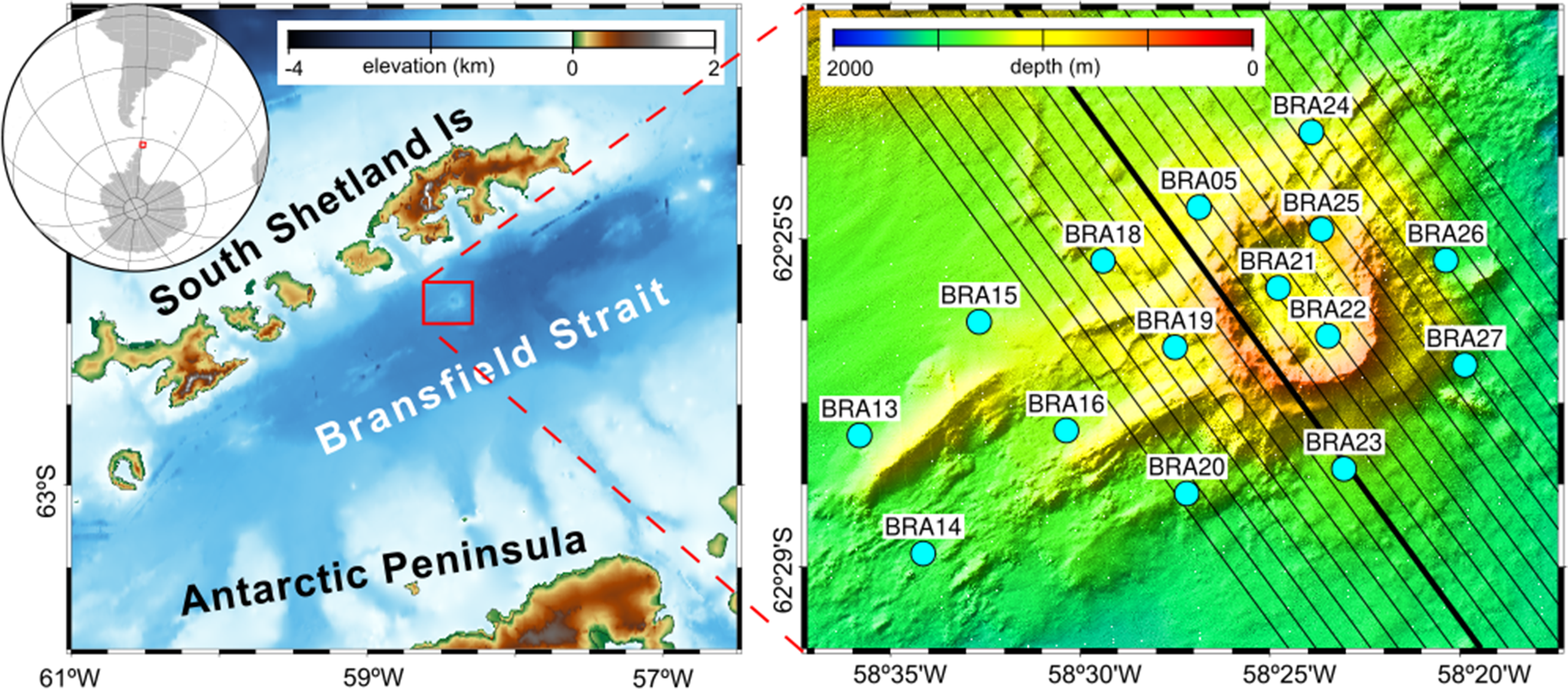
Figure 1. (Left) Map of the Bransfield Strait, indicating the position of Orca volcano between the South Shetland Islands and the Antarctic Peninsula. (Right) Detail of the ocean-bottom seismometer network (cyan dots) deployed around Orca volcano. The black lines indicate the seismic reflection profiles carried out during the BRAVOSEIS 2019 survey using a 1580 cubic inch airgun. The thicker line corresponds to profile OR14.

The BRAVOSEIS project was conducted in 2017–2020 to study the Bransfield Strait volcanoes and the geodynamics of the Bransfield rift. A land-based seismic network was deployed in early 2018, followed by a submarine network in early 2019. The latter consisted of six hydrophones, nine broadband OBSs and 15 short-period OBSs (Almendros et al. 2020). The short-period seismometers had a natural frequency of 4.5 Hz and a sampling rate of 200 samples per second (sps) for the vertical component and hydrophone and 100 sps for the horizontal components. The broadband instruments had 120 s seismometers and recorded at 100 sps (Almendros et al. 2020). Broadband OBSs were deployed with inter-station distances of ~30 km to study regional tectonics and the shallow crust and mantle. Short-period OBSs were spaced densely (∼4 km apart) around the Orca submarine volcano to investigate its seismicity and structure (Fig. 1). These instruments operated from January 2019 to February 2020.

The deployment of seismometers was complemented by seismic reflection and refraction surveys. Gravimetric and magnetic measurements and bathymetric mapping were also carried out (González et al. 2019). During the reflection surveys (Fig. 1), the vessel moved at four knots, and the airguns were placed at a depth of 5 m. Shots were generated every 37.5 m. They were recorded by a 1.5 km streamer, as well as by the seafloor OBS network (Almendros et al. 2020).

Interestingly, the gathered data also contain fin whale calls. The Bransfield Strait is frequented by fin whales for feeding activities (Biuw et al. 2024), especially during the autumn (Dziak et al. 2015, Schmidt-Aursch et al. 2022). Whale calls are recorded by the OBSs as seismic signals with high frequencies (Fig. 2), featuring a high-amplitude initial phase followed by secondary phases. They are best detected on the vertical components and hydrophones, with amplitudes depending mostly on whale distance. The frequency content ranged from 13 to 35 Hz. They appear in series of calls with inter-event spacings of ~15 s (Fig. 2). The series are separated by silences that can last for a few minutes. The reason for these pauses is that whales come to the surface to breathe (Kuna & Nábělek 2021). They then descend and continue singing, and a new series of calls is recorded. These characteristics are similar in other regions (Gaspà Rebull et al. 2006, Wilcock 2012), and they allow fin whale calls to be distinguished from those of other cetaceans (Wilcock et al. 2014, Burkhardt et al. 2021), such as blue whales, with similar dominant frequencies but bi-tonal spectrograms (van Opzeeland et al. 2014), or minke whales (Casey et al. 2022).

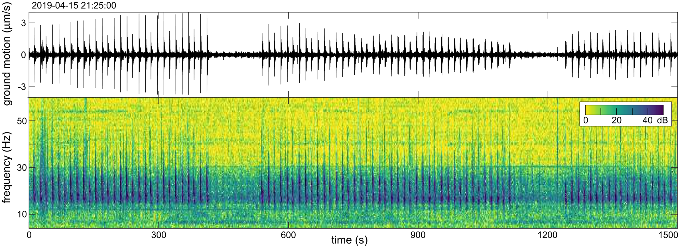
Figure 2. Seismogram (in ground velocity units) and spectrogram showing fin whale songs recorded by the BRA19 ocean-bottom seismometer.

Whale call detection and timing

The use of whale calls for exploration requires the accurate positioning of the whale’s trajectory. We will use a location technique based on the determination of the arrival times of the whale calls. With this aim, we visually explored the dataset, looking for series of whale calls, focusing mostly on the vertical component that had the best signal-to-noise ratio. We selected periods with clear series of calls in a minimum of three stations, without overlapping calls interfering with the detection. These periods occurred mostly during the autumn and extended for timespans ranging from a few minutes to several hours. Stations BRA18, BRA19 and BRA21 were used as references due to the higher number of signals observed in their data. The period from 20h20 to 22h40 on 15 April 2019 was selected for further analysis, as it had very clear signals for a long timespan (Fig. 3).

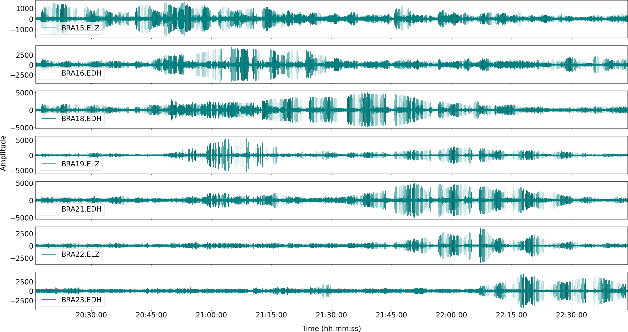
Figure 3. Seismograms (in digital counts) of the time period selected for the analysis (15 April 2019 from 20h20 to 22h40) for representative stations of the ocean-bottom seismometer network. ‘ELZ’ represents the vertical component of the seismometer and ‘EDH’ represents the hydrophone.

The evolution of the amplitudes in Fig. 3 suggests a southwards movement of the whale. The high amplitudes of the signals at BRA15 and BRA16 at the beginning have a decreasing evolution, while at other stations to the south (Fig. 1) the amplitude increases with time. These observations allow us to check the consistency of the results of subsequent analytical steps.

In order to associate the observed arrivals in different stations to a single source, we used the first call following a period of silence. The low propagation velocity and relatively large distances among stations compared to the distance to the whale implies that the travel times to some stations can be similar to the time between calls. This may provoke some ambiguity in the a priori assignation of two records at different stations to the same whale call. By selecting the first call of a series after a silence, we ensure that all records correspond to the selected call. For each of the selected call series, we manually picked the arrival time of the first call, obtaining an initial set of $N$ arrival times ${T}_i^0$ .

We used a relative timing approach based on waveform correlations to obtain the arrival times of successive calls. We could have also obtained manual arrival times for the remaining calls of the series. However, we realized that we could produce better estimates if we exploited the similarity of the waveforms. We selected a time window around the first whale call at each station and used it as a reference template. The template ${P}_i^0$ is initially defined as in Equation 1:

(1) $$\begin{align}{P}_i^0 = {S}_i\left({T}_i^0+ k\varDelta t\right),\kern1em i = 1,\dots, N,\kern1em k = 1,\dots, M\end{align}$$

where ${S}_i$ represents the seismogram at station $i$ , $N$ is the number of stations, $M$ is the number of samples of the template and $\varDelta t$ is the sampling interval. In order to speed up the procedure, we use the seismogram envelope as the input signal, obtained as the amplitude of the Hilbert transform of the data filtered in the 20–40 Hz band. We performed cross-correlations of the template with an $M$ -sample window moving along the seismograms, keeping fixed the relative delays among stations observed in the template. For each step, we obtained an average correlation from all available stations as in Equation 2:

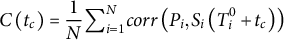(2) $$\begin{align}C\left({t}_c\right) = \frac{1}{N}{\sum}_{i = 1}^N corr\left({P}_i,{S}_i\left({T}_i^0+{t}_c\right)\right)\end{align}$$

To determine the detection of a new call, we define a correlation threshold, established between 0.7 and 0.8 based on a trial-and-error procedure. When the threshold value is reached, a new whale call is declared, and the corresponding time ${t}_c$ is saved as a measure of the delay between the new call and the template call.

However, we need to take into account that the whale moves between calls. In the new call, the relative delays among stations are no longer ${T}_i^0-{T}_j^0$ . They will be different to an extent that depends on the direction and velocity of the whale. Figure 4 shows the evolution of the call envelopes following the template call (in red). To measure the relative delays, we perform a new set of correlations, this time station by station, as in Equation 3:

(3) $$\begin{align}{D}_i\left(\delta \right) = corr\left({P}_i,{S}_i\left({T}_i^0+\delta \right)\right)\end{align}$$

Figure 4. Envelopes of sample whale calls (red lines) and nine successive whale calls (black to grey lines) recorded at the vertical channels of stations BRA18, BRA19 and BRA21. The envelopes represent the energy of the seismogram. The time on the top left indicates the start of the red traces. All calls are aligned at BRA18. At the other instruments, they become progressively shifted in time as a consequence of the movements of the whale.

We define ${\delta}_i$ as the time delay corresponding to the maximum correlation of the template with the new call at station $i$ . In this way, the new arrival times are defined as in Equation 4:

(4) $$\begin{align}{T}_i^1 = {T}_i^0+{t}_c+{\delta}_i\end{align}$$

Although we could have continued this process using the initial template, we realized that the delays and even the waveforms change with time (Fig. 4). Therefore, once we determine the arrival times for the new call, we use the ${T}_i^1$ times of this call to define a new template ${P}_i^1$ . As calls are detected, new templates replace the initial ones to improve ongoing detection. After each new detection, the cross-correlation between the new template and the seismogram is delayed 10 s in order to avoid the seismic coda of the call, whereby different phases such as multiple reflections could produce false triggers in the detection process. In this way, a total of 269 calls were detected during the period of study (15 April 2019, 20h40–22h40). Figure 5 shows the number of locations and the number of stations used for analysing the different sections of the whale song.

Figure 5. Representation of the number of calls detected at different time ranges (vertical bars, left axis) and number of stations used in the location process (orange line, right axis).

It is noteworthy to mention that although the selected times of the first call in a series are obtained manually, the remaining arrival times are calculated automatically based on cross-correlations. In this sense, they are relative locations benefitting from the similarity of waveforms. Although the absolute location has a significant uncertainty that is related to the errors in the manual time selection (approximately the dominant period of the signal: ∼50 ms), the trajectory itself is defined with more accuracy due to the smaller errors in the relative timing process (down to the sampling interval of 5 ms).

Whale location and trajectory

The position of the whale for each call was determined using the arrival times ${T}_i$ measured at a set of $N$ OBS stations. For a whale located at coordinates $\left({x}_w,{y}_w,{z}_w\right)$ and a station located at $\left({x}_i,{y}_i,{z}_i\right)$ , the travel time from the whale’s position to the OBS can be simply estimated as in Equation 5:

(5) $$\begin{align}{t}_i\left({x}_w,{y}_w,{z}_w\right) = \frac{1}{v}\sqrt{{\left({x}_w-{x}_i\right)}^2+{\left({y}_w-{y}_i\right)}^2+{\left({z}_w-{z}_i\right)}^2}\end{align}$$

where $v$ is the acoustic velocity. We assumed a homogeneous water layer with $v$ = 1460 m/s based on the expendable bathythermograph (XBT) results from the BRAVOSEIS survey (González et al. 2019). Although velocity varies slightly with depth, we consider that these variations are not significant for our purposes.

In order to determine the whale location for each call, we defined a grid of 7 × 7 km with a cell size of 50 m. For simplicity, we assume a constant whale depth of ${z}_w$ = 10 m (Wilcock 2012, Kuna & Nábělek 2021). We compute travel times ${t}_i\left(x,y\right)$ from each node $\left(x,y\right)$ to each station $i$ . We calculate the hypothetical origin time ${\tau}_i\left(x,y\right)$ given by Equation 6:

(6) $$\begin{align}{\tau}_i\left(x,y\right) = {T}_i-{t}_i\left(x,y\right) = {T}_i-\frac{1}{v}\sqrt{{\left({x}_w-{x}_i\right)}^2+{\left({y}_w-{y}_i\right)}^2+{\left({z}_w-{z}_i\right)}^2}\end{align}$$

which represents the timing of a call at $\left(x,y\right)$ required for the acoustic wave to reach station $i$ at observed time ${T}_i$ . These $N$ hypothetical origin times for a given location $\left(x,y\right)$ are generally very different from one another. We estimate the origin time dispersion as in Equation 7:

(7) $$\begin{align}\sigma \left(x,y\right) = \frac{1}{N}\sqrt{\sum_{i,j}^N{\left({\tau}_i\left(x,y\right)-{\tau}_j\Big(x,y\Big)\right)}^2}\end{align}$$

The hypothetical origin times will coincide only when $\left(x,y\right)$ is close enough to the real location of the whale causing the call recorded by the seismometers. In such a situation, the dispersion should be close to zero. Therefore, we can estimate the whale location $\left({x}_w,{y}_w\right)$ as the grid point that minimizes the origin time dispersion, as in Equation 8:

(8) $$\begin{align}\sigma \left({x}_w,{y}_w\right) = \min \left(\sigma \left(x,y\right)\right)\end{align}$$

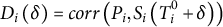
Figure 6 shows a map of the distribution of origin time dispersion for a particular call. The whale location is the point at which the distribution reaches its minimum. The origin time of the whale call is the average of the hypothetical origin times.

In this way, we obtain the position of the whale and the origin time for all of the analysed calls. In order to represent the whale trajectory, some results with larger uncertainties (e.g. when the whale is outside the network area) or corresponding to different, interfering whales were suppressed from the catalogue, so that the 269 calls initially detected were reduced to 194. These points were approximated to a smoothed trajectory, which is representative of the actual path followed by the whale (Fig. 7).

Figure 6. Map view of the distribution of the origin time dispersion (Equation 7) in the selected spatial grid for a sample whale call. The whale location is taken as the point where the dispersion is minimal (the yellow area).

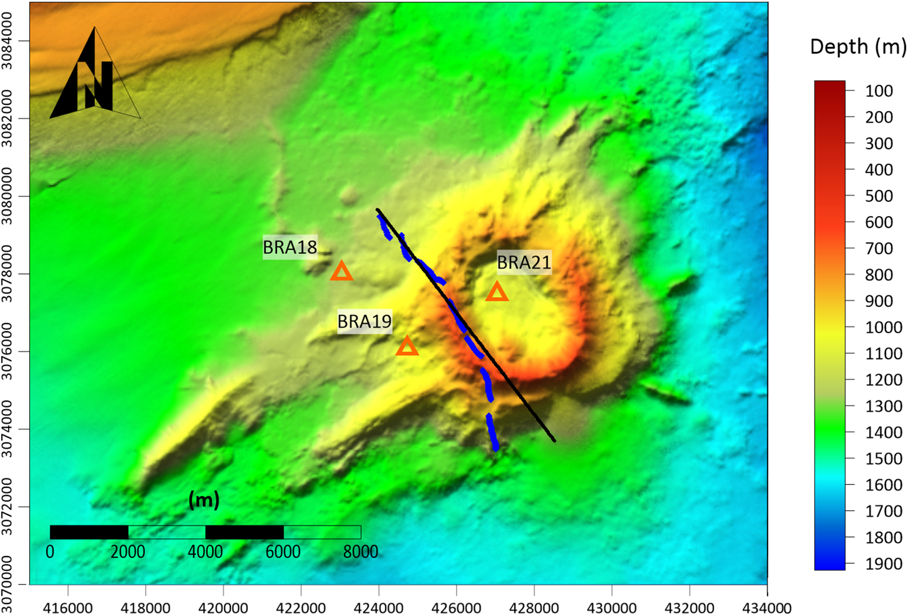
Figure 7. Bathymetric map of Orca volcano, showing the smoothed trajectory of the whale. The black line shows a section of the OR14 seismic profile (see Fig. 1) performed during the BRAVOSEIS seismic reflection study (Almendros et al. 2020). The orange triangles indicate the ocean-bottom seismometer instruments that will be used to compare the seismic signatures of the OR14 airgun profile and whale trajectory (see text for explanations).

The trajectory indicates that the whale approached the Orca crater from the north-west, travelled tangentially to it for some kilometres along the crater rim and then continued southwards. Figure 8 shows the distance travelled by the whale along its path as a function of time. We can see that it moved with an almost constant velocity of 7.2 km/h, a value consistent with other observations (Kuna & Nábělek 2021). As a point of curiosity, the whale’s velocity is quite similar to the speed of the vessel during the seismic reflection surveys, which was 4 knots or ~7.4 km/h.

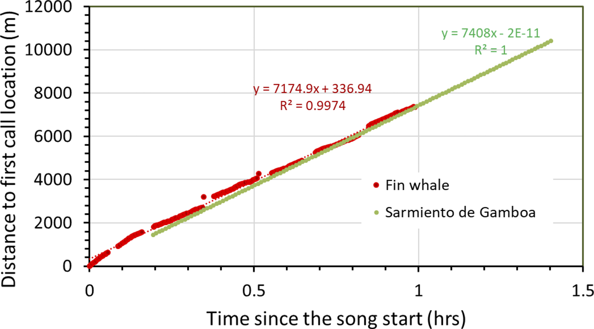
Figure 8. Representation of the distance travelled by the whale as a function of time (red dots). Distances and times are measured relative to the position and origin time of the first call of the series. The dotted red line represents a linear fit, indicating that the whale travels with an approximately constant velocity of 7.2 km/h. The green line represents the velocity of the RV Sarmiento de Gamboa while carrying out profile OR14 during the BRAVOSEIS 2019 survey.

Receiver gathers of whale calls and airgun shots

The whale track identified in the previous section coincides approximately with profile OR14 (Fig. 1), one of the seismic reflection profiles carried out during the BRAVOSEIS 2019 survey (Almendros et al. 2020). Therefore, the convenient situation is that our OBS network recorded overlapping profiles using two different seismic sources: the 1580 cubic inch (c.i.) airgun shots carried out on 23 January and the whale calls from the 15 April excursion of a fin whale across Orca volcano. This coincidence allows us to assess the extent to which the seismic signatures of the fin whale calls can be used for seismic exploration and to compare their performance as seismic sources with the airgun shots.

For this purpose, we generate receiver gathers using both the airgun shots and the whale calls. A receiver gather represents a collection of individual seismic traces from successive sources recorded by a single instrument. Traces are aligned at the source origin time so that the vertical axis represents the travel time of the seismic phases. The horizontal axis usually represents the source-receiver offset. In our case, as the profiles do not cross over the receivers, we define as the offset the distance from the source to the projection of the receiver into the profile (i.e. the closest point of the profile to the receiver). The reciprocity theorem states that these gathers can also be interpreted as being the result of a single source (whale call/airgun shot) occurring at the OBS position and recorded by multiple instruments located at the whale/vessel positions.

We select the three OBSs closest to the whale trajectory for further analysis: OBS18, OBS19 and OBS21 (Fig. 1). We convert the vertical-component seismogram recorded by the OBSs (as a continuous mini-seed stream) into SEGY format. For the airgun shots, timing and coordinates were known accurately from the BRAVOSEIS 2019 survey records (González et al. 2019). For the whale calls, we rely on the estimated locations (described earlier. The receiver gathers were edited using amplitude correction (via automatic gain control) and a bandpass Butterworth filter (10–35 and 10–60 Hz for whale calls and airgun shots, respectively) to enhance weak signals. The resulting seismic gathers are displayed in Fig. 9.

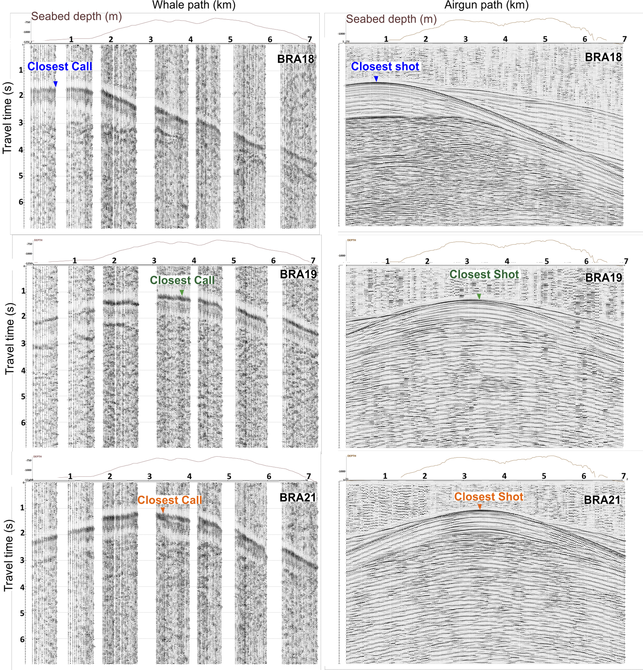
Figure 9. Receiver gathers obtained for the selected ocean-bottom seismometer (OBS) stations using whale calls (left) and airgun shots (right). The vertical wiggling lines are the seismograms recorded by the OBSs for different calls/shots. The horizontal axis represents the distance of the source to the location of the first event of the trajectory. The vertical axis displays the travel time relative to the origin time of each whale call/airgun shot.

We notice a general resemblance between the features observed in the call gathers and the shot gathers. The signal-to-noise ratio is higher for the airgun shots, and the observed arrivals are sharper and better defined. This effect can be related to the character of the source. Airgun arrays are designed to generate pulses with a wide spectrum, whereas whale calls have a narrow-band spectrum produced by a resonance mechanism in the whale’s vocalizing cavities. Figure 10 shows a comparison of the waveforms and spectra of several airgun shots and whale calls recorded at BRA19. The airgun source produced signals with significant energy in the 5–80 Hz band, whereas the whale calls are essentially limited to the 15–25 Hz band.

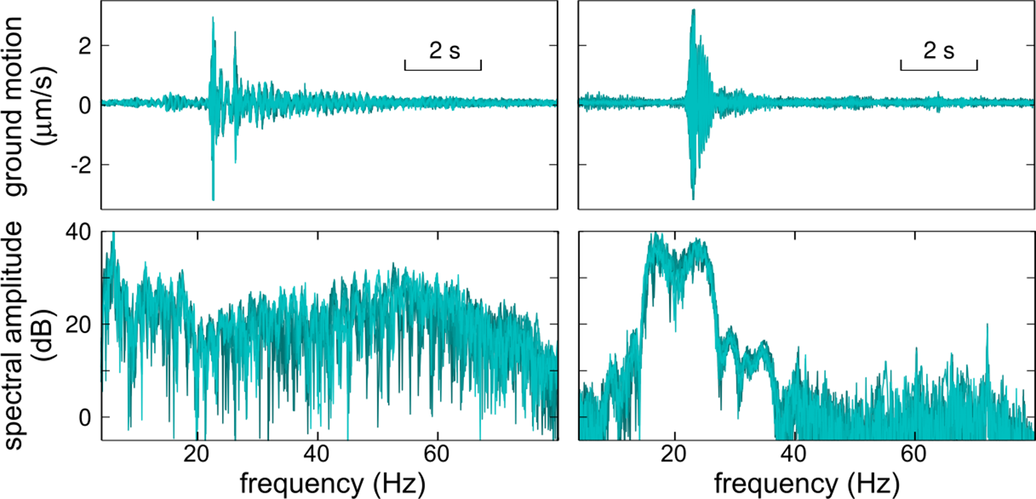
Figure 10. Seismograms (top) and spectra (bottom) of airgun shots (left) and fin whale calls (right) recorded at the BRA19 ocean-bottom seismometer. The shades of cyan correspond to eight different signals of each type.

Additionally, the call gathers show small temporal jerks from one call series to the next, with magnitudes of up to ∼0.2 s, in contrast with the smoother appearance of the shot arrivals. These jerks can be attributed to uncertainties in the whale’s location. Determinations of the call origin time and location are intertwined, and the uncertainties in the arrival times (which are obtained manually for the first call of a series) can lead to errors in both location and origin time.

Interpretation of the receiver gathers

Comparison of seismic phases

In order to identify and interpret the seismic phases, we should take into account the fact that the receivers are offset from the source trajectory, and therefore the seismic ray paths display a fan geometry that spans a relatively wide area. In a flat-layered structure, this fact would have no further consequence; however, in a heterogeneous medium, the seismic energy generated by different sources does not propagate through the same structures. It interacts with layers and topographies that may be different for each source position, and therefore the interpretation becomes more challenging. Here, we will take a simplistic approach, assuming that the receivers are close enough to the source profile and that the structure is sufficiently similar to a flat-layered structure.

An acoustic source generates energy that propagates to the OBS following different paths that produce a variety of seismic phases (Fig. 11). The direct wave (Dir) travels in the water layer from the source to the sea floor. Acoustic energy is also reflected at the sea floor and again at the surface, generating the first multiple (ML1) and possibly other guided waves. Additionally, if we assume a simple layered structure with a sediment layer over hard rock (probably volcanic materials), several other phases are to be expected as well. The transmitted energy travels through the sediment unit to the basement, where reflected (Rx2) and refracted (BR, R3) waves are originated.

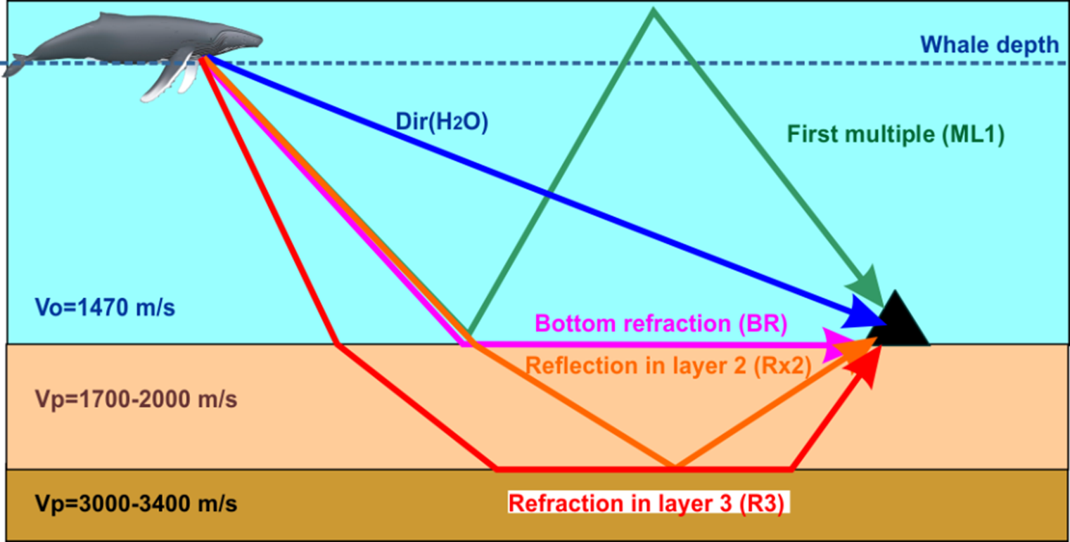
Figure 11. Sketch illustrating the ray paths of the main acoustic and seismic phases that can be generated by an acoustic source (whale call or airgun shot) in a flat-layered structure. The velocities of this model have been deduced from the analysis of the seismic gathers. Dir = direct wave; Vo = velocity of acoustic waves in the ocean; Vp = velocity of the P-wave in the seafloor layers.

Figure 12 shows the identification of seismic phases in the receiver gathers. There is a remarkable correspondence between the phases detected in the airgun shot gathers and the whale call gathers. In both cases, the direct waves (blue) and multiples (green) have the highest amplitudes and can be readily identified. We can also detect a second multiple in BRA21. In addition to the waterborne waves (layer 1), we identify other seismic phases related to wave reflections and refractions in the sedimentary unit (layer 2) and in the lower compact unit (layer 3). The interpretations and estimates of apparent velocities are based on the shot gathers as they have more energy, wider bandwidths and a constant spacing between traces, although we mark equivalent observations in the call gathers.

The best match between the call and shot gathers occurs for BRA19, for which the call gather shows most of the phases identified in the shot gather. In the other cases, some of the fainter phases are not easily identified in the call gathers.

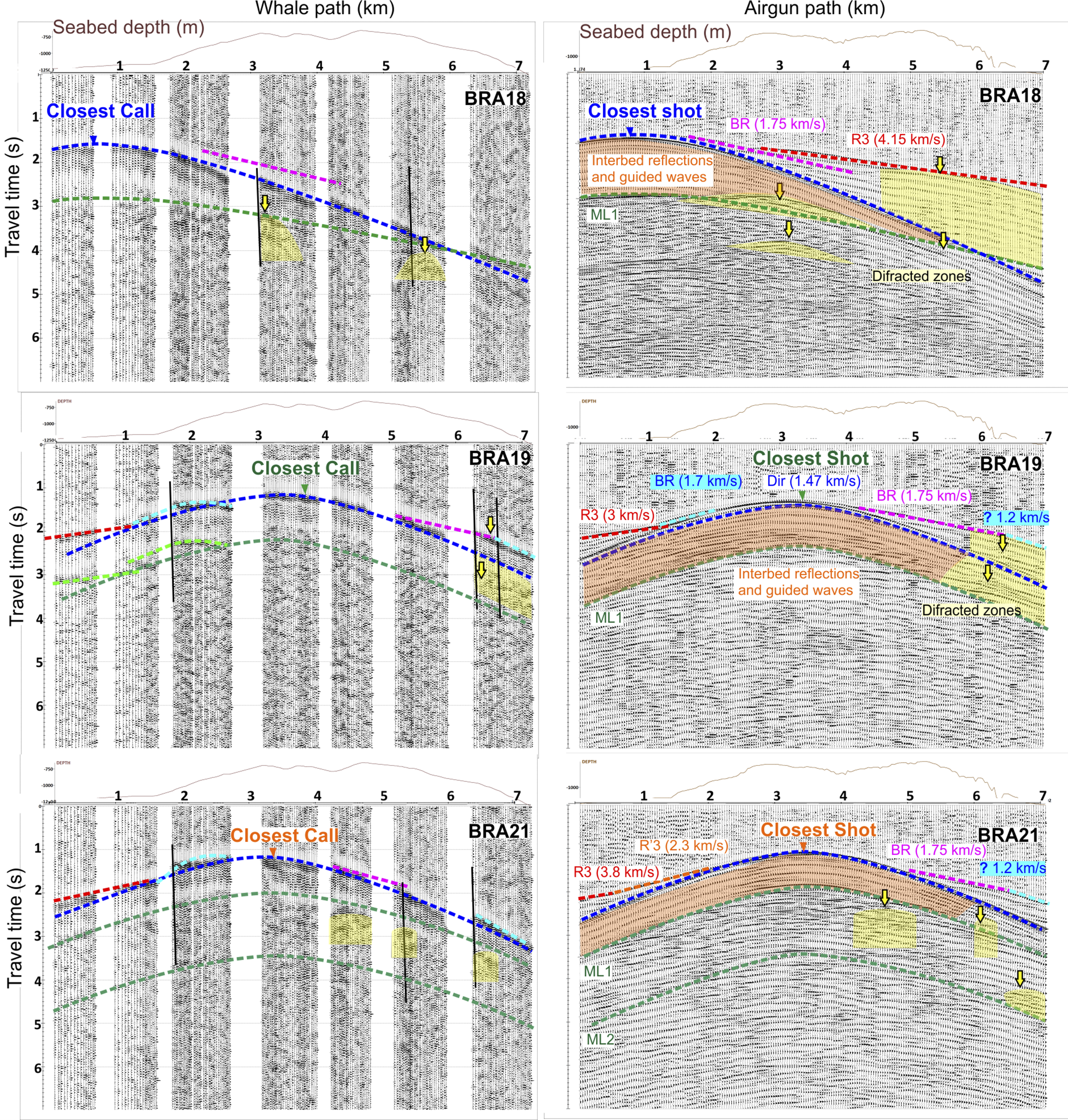
Figure 12. Interpretation of the seismic phase arrivals observed in the whale call gathers (left) and airgun shot gathers (right). The figure layout is the same as in Fig. 9. The different colours indicate seismic phases corresponding to the simple scheme of Fig. 11 (see text for explanations).

The direct wave has an apparent velocity of 1.46 km/s, as expected according to the XBT measurements taken during the BRAVOSEIS cruise (González et al. 2019, Almendros et al. 2020). The seafloor refractions (cyan, magenta) propagate with velocities in the range 1.6–2.0 km/s, which may correspond to sediments (lower velocities) and marine sediments mixed with lava flows (higher velocities). The refraction in layer 3 (red) suggests a higher velocity of 3–4 km/s, consistent with compact materials related to the Orca volcano edifice. We also observe inter-bed reflections and guided waves, with arrival times falling between the direct arrival and the first multiple. Finally, we observe areas with diffractions, especially in the southern-most parts of the whale and vessel paths. We attribute these diffractions to the complex topography along the source-receiver path.

For the receiver gathers with centred receivers (BRA19 and BRA21) the coincidence is greater because we detect refracted waves at both sides of the direct wave arrivals (central part; blue in Fig. 12). In the north-western part of the trajectory (left side of Fig. 12), we see two phases with velocities of 1.7 km/s (BRA19) and 2.3 km/s (BRA21) that in the call gathers have a time jump (black line) of ~0.3 s, coincident with a breathing gap. This could be due to the uncertainty in establishing the origin time of the initial call. Towards the end of the profile, phases with similar apparent velocities to those in the shot gathers are observed. In the south-eastern part, we see the refraction corresponding to sediments (1.75 km/s) and a final anomalous region with a velocity of 1.2 km/s. In the BRA21 call gather, this low-velocity layer is not detected. This part of the source path is located beyond the southern rim of the Orca crater, where the topography and structure are most different from our simplifying hypothesis of a flat-layered structure. In this region, we observe diffraction structures (yellow areas in Fig. 12), in both the call and shot gathers. In this volcanic environment, diffractions may occur not only due to the topography, but also in relation to fractures and dykes. In the shot gathers, we observe multiple reflections within the sediment layer (orange area in Fig. 12) between the direct wave and the first multiple. Finally, for BRA21, we are able to see a second multiple in both the shot and the call gathers.

Approximate velocity models

We have estimated three approximate velocity models combining the information from the shot and call gathers. For this task, we used the critical distances and times corresponding to the points where seismic phases refracted at different layers arrive simultaneously (Xc,Tc). As explained earlier, we assume two important simplifying hypotheses: 1) the receivers are close to the profiles, so that we can consider that they travel through somewhat similar structures; and 2) the medium can be approximated by a flat-layered structure. This second assumption is feasible when the subsoil consists of parallel layers and the seafloor relief is relatively flat. However, in this area, the relief of the seabed is steep, and the sensors are located on the slopes of a volcano. Therefore, we are conscious that this is a crude approximation, and it is performed not to produce a credible model of the shallow crust but mostly to compare the performance of the whale call gathers with the airgun shot gathers.

Figure 13 shows a sketch of the derived models. We used the space-time distribution of direct and refracted waves observed in the shot gathers to determine the model geometry and velocity. The features marked with a yellow diamond can be also obtained using the whale call gathers alone. The area where the direct wave arrives first is represented by a blue ellipse. Then we have other waves refracted in the sediment layer and in the basement. All stations reveal a low-velocity region at the south-eastern end of the profile. Velocity values and layer thicknesses are not symmetric with respect to the central shot/call, although the modelled structures are generally consistent. The 5.2 km/s layer in BRA18 has lower velocities of 3.0–3.5 km/s in the other models, which again indicates the probably heterogeneous structure of the medium.

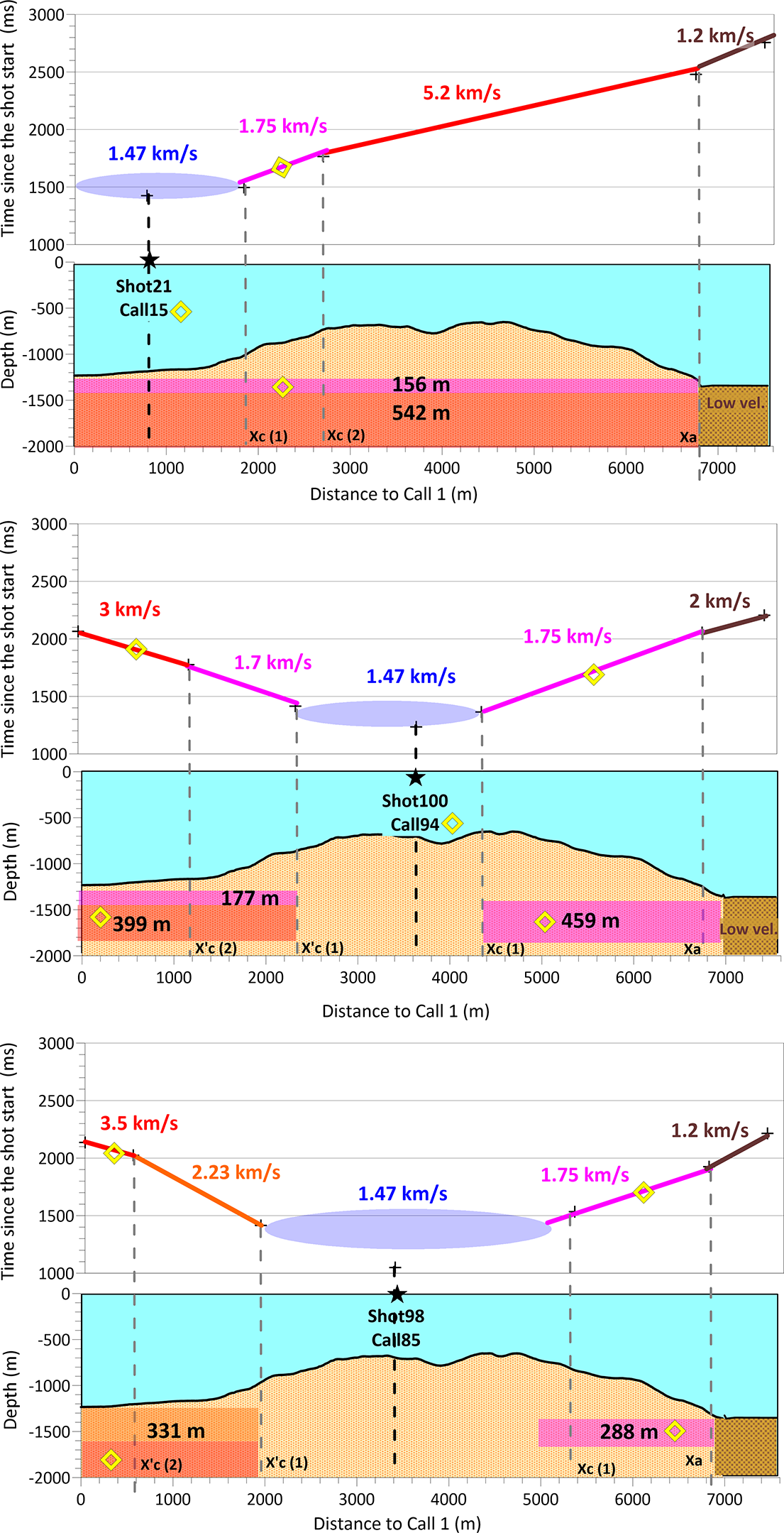
Figure 13. Representation of the approximate velocity models obtained from the airgun shot gathers for ocean-bottom seismometers BRA18 (top), BRA19 (middle) and BRA21 (bottom). In each panel, we represent at the top the travel times of the direct and refracted arrivals as a function of source offset, with an indication of the seismic velocity of the layers. At the bottom, we show the critical distances Xc and thicknesses of the detected layers, as well as the topography of the sea floor under the source profile. The black stars indicate the positions corresponding to the calls/shots closest to the receiver. Yellow diamonds indicate the features that are also revealed by the analysis of the whale call gathers.

In any case, by using the call gathers we can identify most of the features of these models. For example, in BRA18 we image a sediment layer over the basement and a low-velocity zone. The BRA19 and BRA21 models would be also well reproduced, except for the first unit in the north-western part of the profile. However, we could still model the basement to an adequate depth.

Discussion and conclusions

We have used stations from an OBS network to detect and locate whale calls in the Bransfield Strait, Antarctica. This method is based on the manual determination of arrival times and location of the first call of a series, followed by an automated detection and location algorithm exploiting the similarity of waveforms between successive calls. This approach allows us to determine the trajectory of a whale accurately, although its absolute location still has a relatively large uncertainty. This could be the reason for the apparent jumps in the receiver gathers using whale calls.

We have carried out a simplistic interpretation based on the hypothesis that the geometry of this problem can be approximated to a fan shot gather and that the distribution of velocity in the medium is sufficiently close to that of a flat-layered structure. Although the derived velocity structure may be biased by these assumptions, it is still consistent with the structures imaged in refraction studies in the area (Barker et al. 2003, Christeson et al. 2003). It is also consistent with the results of Kuna & Nábělek (2021) using fin whale calls in the North Pacific. The analysis could be improved by using the bathymetry to generate synthetic waveforms under different conditions and to reproduce the recorded waveforms. Other improvements could include automating call detection and location with machine learning, using advanced relocation methods or employing additional techniques such as seismic interferometry.

Our study corroborates the notion that whale calls can be used for shallow exploration of the sea floor, as proposed by Kuna & Nábělek (2021). The main advantage of this approach would be that this type of source has virtually no environmental impact. When compared to an airgun source, it still has reasonable resolution for short offsets, and we have found that the whale call spacing and timing are similar to those of a standard seismic airgun profile. However, there are some drawbacks that may limit the usability of this approach. Firstly, whales are unpredictable sources that may or may not provide data when and where we wish. This is an obvious complication compared to controlled artificial sources. Therefore, such calls might only be useful in areas frequented by whales and with long-term OBS deployments. Secondly, the fin whale call spectrum has a narrower band compared to airgun signatures, which reduces the sharpness and resolution of the seismic images. In addition, these calls are usually less energetic, which limits the depth of exploration that they allow. The lack of low-frequency energy is also a limiting issue with respect to the depth of investigation.

In any case, although the use of fin whale calls cannot fully replace professional marine seismic surveys, it provides a valuable complementary tool and a passive source of information regarding areas under research. Additionally, seismic information could be useful in marine biology to help constrain and characterize whale behaviour. This work represents a simple attempt at exploring research methods with less of an environmental impact, which allow the advancement of scientific knowledge while respecting and conserving natural resources.