Successful deployment of a large uncrewed aerial vehicle for multidisciplinary science from Rothera Research Station, Antarctica: 2024 season overview and lessons learned

Abstract

Airborne investigations are a keystone for understanding the Antarctic environment across many scientific disciplines. Over the past decade and more, the use of drones has been proposed as a means to enhance this airborne capability. Small quadcopter/multi-rotor drones, typically flown within visual line of sight, have become a well-established and routinely deployed technology. However, larger fixed-wing uncrewed aerial vehicles (UAVs) capable of beyond-visual-line-of-sight missions similar to traditional crewed aircraft have not been routinely deployed. Here, we report on the first deployment of a large (10 m wingspan) UAV for scientific data collection from Rothera Research Station, Antarctica. The platform, a Windracers Ultra, flew 2978 km over 25 missions, collecting a range of scientific observations including visual and hyperspectral imagery, atmospheric turbulence data and gravity and magnetic data. All science missions were carried out beyond visual line of sight and were up to 2.25 h/260 km long. Missions included coordination with and operation alongside crewed aircraft. Our field season has successfully demonstrated that large UAVs can play a significant role in Antarctic data collection, working alongside crewed aviation to improve our understanding of Antarctica.

Introduction

Antarctica is the least understood continent on our planet due to the logistical challenges of working in this remote and extreme environment. Significant advances remain to be made across disciplines as diverse as tectonics, cryosphere science, meteorology and ecosystems in this region. Collection of scientific data in Antarctica is of particular importance as we try to observe, predict and mitigate the impacts of climate change. Airborne surveying has become a mainstay of Antarctic environmental science, as it can deliver high-resolution data from some of the most remote regions on Earth, yet it presents its own challenges, including delivering the volumes of fuel required for surveying, the direct CO₂ overheads associated with survey flying, gaining access to aircraft committed to multiple logistical and scientific roles and restrictions due to field season operational windows.

Uncrewed aerial vehicles (UAVs) have been proposed for several decades as alternative or additional platforms that can deliver airborne science data while reducing many of the challenges faced in such work. UAVs are typically significantly smaller than traditional aircraft, therefore requiring less direct fuel burn per kilometre flown, hence presenting a lower logistical overhead. As lower-cost platforms, UAVs can also be easier for researchers to access than traditional aircraft. Despite the promise of UAVs for Antarctic science, they have not become a mainstay of regional (tens to hundreds of kilometres) airborne science data collection, with UAV developments mainly focusing on quadcopter-type platforms for local observations (0.5–10 km range; Pina & Vieira 2022). The main challenges facing regional scientific data collection using UAVs have included their size and the power consumption of payloads, the cost of UAV platforms capable of data collection over long ranges and issues associated with the integration of UAV operation with crewed aviation. Recent advances in sensor technology, reducing their weight and power consumption, coupled with advances in civilian drone design, including improved range, payload capacity and operational procedures, now make UAVs a realistic platform for regional Antarctic scientific data collection.

Many examples of both quadcopter-type and fixed-wing UAV use in Antarctica are presented in the review paper by Pina & Vieira (2022). Early examples of regional fixed-wing UAV use included collection of atmospheric data around Halley Research Station using a M²AV device with a maximum take-off weight (MTOW) of 5.0 kg (1 kg payload) and a range of ~50 km (Spiess et al. 2007), reported in a British Antarctic Survey (BAS) press release (18 March 2008, No. 09/2008, https://www.bas.ac.uk/media-post/unmanned-aerial-vehicles-mark-robotic-first-for-british-antarctic-survey/). Longer-range missions conducted with a fixed-wing platform include aeromagnetic flights over Deception Island, in which 303 km of data were collected in a single mission (Funaki et al. 2014). The platform used had a MTOW of 28 kg, with a payload of up to 2 kg. Although demonstrating the potential of UAVs for regional survey, this study highlighted issues associated with scheduling UAV operations alongside crewed aircraft, and subsequent loss of the platform further demonstrated the challenges of Antarctic UAV operation. More recent collection of airborne radar data using a G1X UAV, which has a 39 kg take-off weight and ~9 kg payload (Leuschen et al. 2014), demonstrated the diversity of Antarctic science data that can be collected using a UAV platform. Although each was successful in its own way, these examples have not yet led to the routine adoption of UAVs for regional airborne data collection.

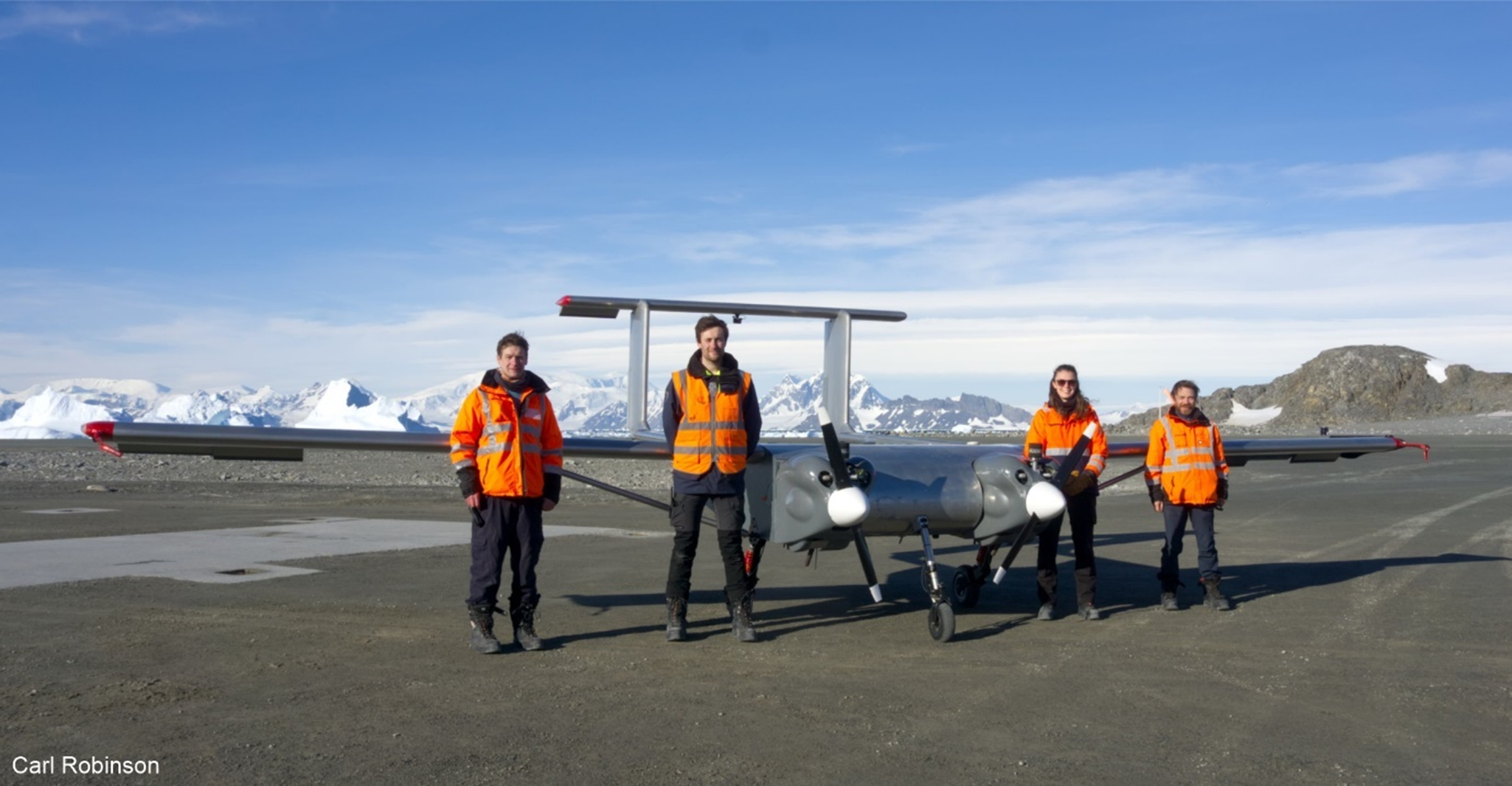
Figure 1. SWARM survey field team, with the Windracers Ultra TD-2-01 uncrewed aerial vehicle at Rothera Research Station.

To progress development of the civilian UAV business sector, including environmental protection and monitoring, Innovate UK, the UK’s national innovation agency, a division of the UK Research and Innovation (UKRI) funding body, put forward its phase 3 Future Flight Challenge. Working in collaboration, Windracers Ltd, Distributed Avionics Ltd, Helix Geospace, Lancashire Fire and Rescue Service, the University of Bristol, the University of Sheffield and BAS developed the ‘Protecting environments with unmanned aerial vehicle swarms’ project, known as SWARM. The aim of this project was to demonstrate how the Windracers Ultra UAV and swarm technology can conduct environmental protection missions, including the detection and location of wildfires and gathering environmental data in Antarctica. To prove that the Ultra UAV was suitable for a range of environmental protection and monitoring tasks in Antarctica and beyond, it was important for a range of meaningful scientific datasets to be collected. A call was therefore placed within BAS for appropriate airborne survey missions that could deliver useful scientific data while operating from the BAS Rothera Research Station. Missions including measuring atmospheric turbulence, observing remote Antarctic Specially Protected Areas (ASPAs) using visual and hyperspectral data, collecting airborne magnetic and gravity data for tectonic studies and collecting airborne radar data were planned to be delivered over a 6 week field season from January to March 2024. Here, we provide an initial overview of the platform, payloads and scientific data processing from across this field season.

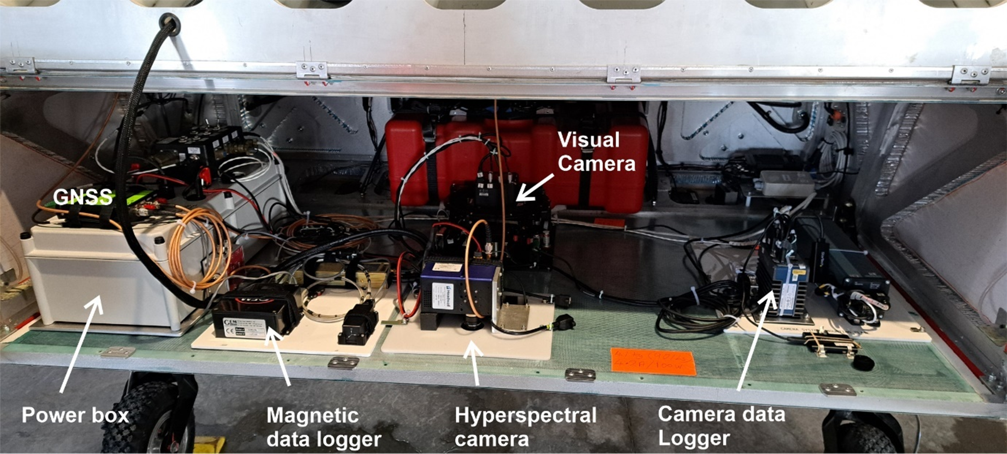
Figure 2. Camera floor installed in Windracers Ultra, looking forward. Note that the entire floor area could be installed/removed when populated with scientific equipment.

Table I. Floors fitted to the Windracers Ultra platform. Note that weights exclude enclosures/mounts and cables.

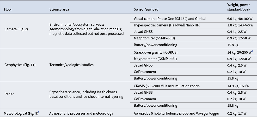
^a Peak power for the gravity system is specified by the manufacturer and only applied during initial warm-up of the system in the laboratory prior to installation.

^b Meteorological fit was not on a floor and was carried on all scientific missions.

Platform

The original design concept for the Windracers Ultra UAV (Fig. 1) was for a cargo drone capable of delivering 100 kg of cargo over ~1000 km. It was specifically conceived to provide essential logistical support to humanitarian agencies looking to sustain communities through emergencies where transportation links are poor. This design concept has led to a robust and easy-to-maintain UAV platform with a large and easily accessible rectangular payload area. The payload bay has a volume of 700 l and up to 350 W of available electrical power, features that make it a good candidate for an Antarctic survey platform. The aircraft that was deployed was an early prototype Technology Demonstrator (TD2-01) with a 10 m wingspan, an empty weight of 285 kg and a MTOW of 380 kg. It can operate from ~150 m-long runways in wind speeds of up to 40 knots, and it has a range of ~400 km with a payload of up to 100 kg. Current production examples have a higher MTOW of 500 kg, a higher payload capacity and a longer-range capability due to larger fuel tanks, and these could be employed for future deployments. For this deployment to Antarctica, the platform and all associated spares and ground infrastructure were packed into a standard 20 ft shipping container, which was delivered to Rothera Research Station via the Natural Environment Research Council (NERC) Sir David Attenborough research vessel.

To integrate potentially complex scientific payloads without significant modification of the platform, we developed a removable floor concept (Fig. 2). The standard floor of the Ultra is an 82 × 178 cm composite panel constructed from high-density foam around aluminium reinforcing struts. Inside it provides a flat floor, while the outside has an aerodynamic curve covered by an aluminium skin. This floor is fixed to the aircraft frame at six relatively easily accessible attachment points, meaning it is easy to remove and replace. We therefore constructed additional bespoke floors with appropriate apertures and equipment fixing points for each scientific payload (Table I). These floors followed the attachment pattern of the standard Ultra floor design, meaning that they could be populated outside the aircraft and simply be slotted in and bolted to the Ultra frame as required, replacing the standard floor.

The magnetic sensor and turbulence probe could not be attached to the main floor, meaning additional mounting schemes were developed. The turbulence probe was fitted within a 3D-printed housing attached to the port wingtip, replacing the navigation lights. Power was supplied via the feed to the navigation lights, and the sensor had its own dedicated Global Navigation Satellite System (GNSS) antenna fixed to the printed housing. The magnetic sensor was mounted in the payload bay door of the Ultra, meaning the sensor sat ~1.5 m behind the payload bay when the door was closed. This location was chosen as other areas far from the core electronic systems and engines, such as wingtips and tail, housed electronically activated control surfaces, which would probably generate unacceptable levels of noise. The magnetic sensor was mounted vertically in a 3D-printed bracket that attached to the upper and lower aluminium skin of the door using nylon bolts.

Power for the survey instruments came from two potential sources: the aircraft or a 24 V lithium battery. The power was diode consolidated to give uninterrupted 24, 12 or 5 V supply to the scientific equipment (Fig. 2). The configuration of the power conditioning gave priority to the use of aircraft power when available but fell back onto the battery when aircraft power was off. This design allowed the scientific equipment to be powered independently of aircraft systems in preparation for take-off and during data download after landing. This system also removed any in-flight constraints on the Ultra Ground Control Station (GCS) operator (the de facto pilot) if they felt there was an operational requirement to remove survey power.

Positional information for the scientific equipment came from two dedicated GNSS antennae mounted on the top of the Ultra fuselage, adjacent to the antennae used by the Ultra itself. One of the antennae, offset to the port side of the platform, was connected to a Javad Delta receiver, which logged positional information on most missions. This antenna was also connected via a splitter to the magnetometer data acquisition system, which includes its own basic GNSS receiver. The second antenna, which was positioned on the centreline of the platform, was attached to either the Headwall Hyperspectral camera, which includes a Trimble Applanix Inertial Navigation System (INS) and GNSS receiver, or to the iMAR gravity sensor with integrated NovAtel GNSS receiver, depending on the mission payload. Data from the central antenna are preferred for post-processing; however, the data recorded by the Javad receiver provided redundancy in case of issues with the other system, together with timestamp information for systems without internal GNSS capability.

The deployed camera, hyperspectral and radar systems collect large volumes of data and were therefore only triggered to collect data when over relevant target areas. For the visual camera and radar system, triggering utilized an output from the Ultra’s guidance system. This output included an optional servo command (high or low voltage) when the platform reached a designated waypoint. This voltage change was then used to switch on/off the camera or radar system. The GCS operator could also update the servo state in flight, turning these systems on/off at will. The hyperspectral system relied on its own dedicated GNSS feed, coupled with ‘geo-fenced’ areas loaded before each flight. Whenever the platform entered a geo-fenced area, data would be collected, and data collection stopped when the platform left the area. Other systems, including GoPro cameras, gravity and magnetic systems and the wingtip turbulence probe, were switched on to record before the flight and were shut down after landing.

Operations

The Ultra could be directed/controlled by two distinct operators: the GCS operator, who for this survey was located in an office in Rothera Research Station, or the safety pilot, who was stationed adjacent to the runway when appropriate. Flight operations were split into three distinct phases: take-off and initial visual line of sight (VLOS), beyond VLOS (BVLOS) and final VLOS and landing. During VLOS operations, the platform was within 1.5 km of the safety pilot, who could intervene and direct or take full manual control of the platform via a handheld remote control (RC) unit. Although such intervention was possible during the VLOS phase of the missions, it was not required on any routine missions during this season, with platform control remaining with the Ultra autopilot directed by the GCS operator. The ability of the safety pilot to direct the platform was used during magnetic sensor calibration (see ‘Gravity and magnetics’ section). During both VLOS and BVLOS operations, a radio-link from a transmitter on Rothera Point, routed via the station-wide intranet to the GCS, was used to communicate between the GCS and the platform.

During a typical mission, the GCS operator directed the Ultra by uploading pre-planned missions. These included a take-off mission, the main BVLOS scientific mission and a landing mission. An additional emergency return route, avoiding significant terrain and returning to a loiter point within VLOS range, was also uploaded in case of unexpected communications failure. This emergency flight path was automatically enacted after a set amount of time of lost communication, but it could be overridden once communication was restored. Where missions needed to be curtailed for other operational reasons, the GCS operator directed the platform to bypass the most distant waypoints. In some cases, the science mission took the Ultra into areas with no radio communication due to the shadowing effects of elevated topography. Such missions were pre-planned, and ~5 min before the period of lost communications the platform was directed to continue its primary mission in case of any loss of communications. The longest period of lost communication due to this type of operation was ~16 min.

Specific environmental operational limits were defined prior to the field season. A maximum crosswind component of 20 knots and a total maximum windspeed of 30 knots were prescribed during take-off/landing. During flight, a maximum wind speed of 40 knots was mandated. VLOS operations were restricted to where visibility was > 1 km and the cloud ceiling was ≥ 500 ft above ground level (AGL) or higher. The limit for maximum precipitation was light (< 2.5 mm/h). For all survey missions, marginal wind, precipitation and visibility conditions were avoided. In addition to these parameters, icing conditions pose an operational risk to all aircraft, and the Ultra platform is no exception. Survey missions were therefore not launched to BVLOS areas where weather forecast models or direct weather observations suggested cloud at the survey altitude, as this could indicate an increased icing risk.

Communication is a key part of all crewed and uncrewed aircraft integration operations, and for the Ultra this included three separate and complementary strands. The first and most important operational link was standard voice over radio communications. The controller and point of contact for Ultra was the GCS operator. They were in contact with and directed the safety pilot during initial start-up, ground checks and taxi procedures via a private very-high-frequency (VHF) radio link. The GCS operator communicated with the Rothera tower air traffic coordinator via air band VHF radio regarding weather, other aircraft movements, ongoing mission status and runway/apron status for engine start, take-off and landing. Where required, the Rothera tower passed messages from other aircraft to the GCS operator - for example, advising the GCS operator to change hold location. The second strand of communication was electronic conspicuity. The Ultra was equipped with MODE-S out and ADS-B in electronic conspicuity. This made the platform electronically visible to other aircraft with appropriate receivers and provided the GCS operator with real-time information regarding the location of other ADS-B-equipped aircraft within range of the UAV. The third and final strand of communication was the Distributed Avionics Cloud Control/monitoring system. This allowed the map and mission information from the GCS to be observed on any internet-connected computer that had been given access to the portal. This system was used by the Rothera tower to monitor the missions, including expected time of arrival (ETA), and by the science lead to monitor mission progress and download basic telemetry data.

Missions and flown sensors

Across the 2024 field season (26 January–8 March) we conducted in total 25 flights (Figs 3 & 4). These included logistical/operational integration missions (4 missions), testing an atmospheric turbulence probe (2 missions), photographic surveys of ASPAs (7 missions) and joint gravity and magnetic missions assessing the regions tectonic structure (12 missions). In total, we flew for 26.25 h, covering 2979 km, with a total fuel burn of 254 l of petrol (see Table II).

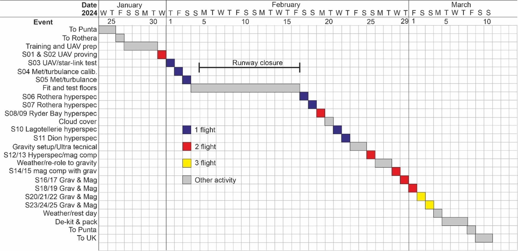
Figure 3. Operational timeline. Horizontal scale indicates date and vertical scale indicates activity. Note that the period of runway closure was for scheduled maintenance. This time was used for ground testing. UAV = uncrewed aerial vehicle.

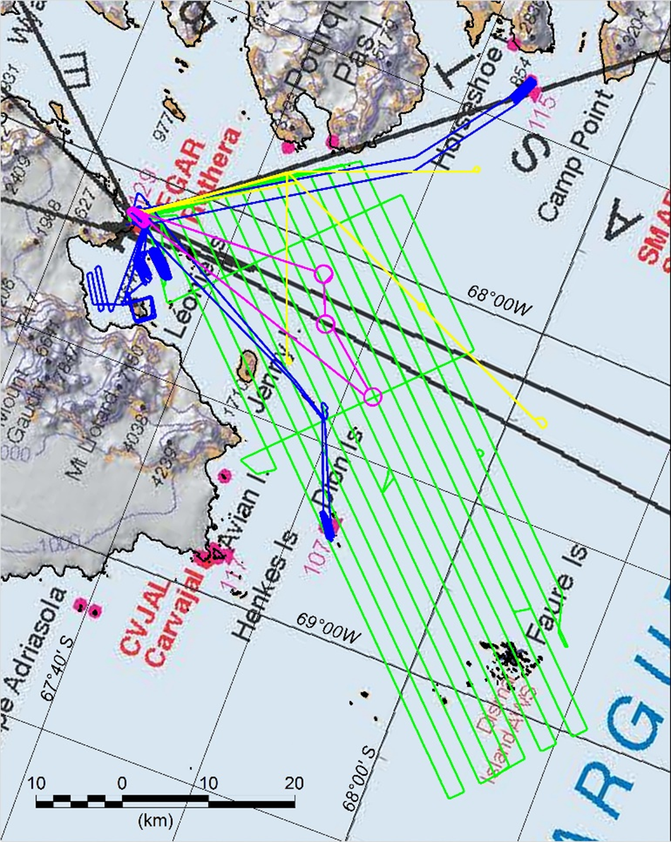
Figure 4. Completed SWARM survey flight lines. Pink = initial testing and operational integration. Yellow = dedicated meteorological flights. Blue = camera and hyperspectral flights. Green = gravity and magnetic flights.

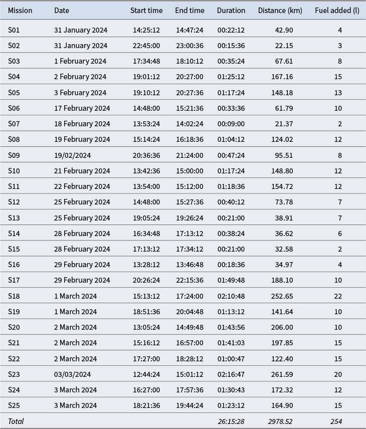
Table II. SWARM flight statistics. Note that fuel added may not be directly proportional to specific flight length due to fuel tank capacity carried over from previous missions and ground testing. The total volume of fuel used across the survey is correct.

Logistical/operational integration missions

These missions aimed to prove platform capability but had no direct scientific objectives (Fig. 4). The first two operational missions were short (15–20 min) VLOS shake-down flights after the Ultra had been assembled to ensure all systems were operating as expected and to confirm initial communication protocols with the Rothera tower (S01 and S02). The third operational mission (S03) was to test whether the Ultra could be operated directly via an onboard Starlink satellite communications system communicating via Distributed Avionics Cloud Control rather than using the standard GCS radio link. This test proved successful, but due to the weight and power consumption of the prototype system it was removed and not used for the subsequent missions.

The final operational integration mission (S18) was designed to demonstrate airspace integration and test procedures for UAVs to be flying at the same time as crewed aircraft. Prior to this point, the UAV had remained grounded while aircraft were in-bound to Rothera, restricting operations. This mission was planned in detail between the BAS chief pilot, the UAV operational team and the Rother tower coordinator, including discussion of the type and likelihood of potential failures and appropriate mitigations. For this mission, the Ultra took off ~1 h prior to the arrival of an in-bound Dash-7 air-bridge passenger flight. Shortly after the Ultra took off, the Dash-7 reached its point of safe return (PSR) and was committed to landing at Rothera. The Ultra assumed a series of hold positions 10 nautical miles from Rothera, simulating the location of a scientific mission. The Windracers Ultra was electronically visible to the Dash-7 crew via Traffic Alert and Collision Avoidance System (TCAS) and the Dash-7 was indicated on the GCS screen via the Ultra’s ADS-B receiver. During the approach, the Dash-7 pilot requested that the Ultra move to a different hold location farther from Rothera. This message was passed via the Rothera tower air coordinator, and the GCS operator repositioned the uncrewed system as directed. As soon as the Dash-7 landed, the Ultra was directed to return to Rothera and the test mission was successfully concluded. This mission demonstrated the high degree of confidence in the platform and its operation gained by the BAS air unit over the season. Further air integration and development of operational procedures will build on this starting point.

Photographic and hyperspectral missions

A key potential use for UAVs is ecological survey and monitoring using visual or other camera systems. Many areas of Antarctica are environmentally sensitive and host unique, rare or endangered ecosystems. Areas of especial significance have been designated as ASPAs under the Antarctic Treaty, and proposing organizations such as BAS have a duty to monitor and maintain these areas. To test whether ASPAs can be monitored using long-range UAVs, we selected a number of ASPAs between 5 and 50 km from Rothera. Each of these areas was overflown by the Ultra with the ‘camera floor’ fitted (Fig. 2). The sensors deployed on the camera floor can also theoretically be used to assess marine areas for the presence of krill (the shrimp-like marine invertebrates that form the base of the Antarctic food chain; Belcher et al. 2021) and glacial out-flow containing eroded sediment (Pan et al. 2023). For this reason, camera and hyperspectral data were also collected over open marine areas on transits to and from ASPAs and along local glacier fronts.

The first key sensor on the camera floor was a visual (RGB) camera system for airborne mapping, including digital elevation model (DEM) generation and the creation of seamless orthorectified mosaics. The camera used was a Phase One iXU 150 medium-format camera mounted in a Somag CSM-130 gimbal. The gimbal ensured that the camera was always pointing vertically down and aligned with the flight track, ensuring adequate and consistent overlap between each swath of images. This system was installed in the forward centre of the payload floor, approximately centred under the GPS antenna linked to the adjacent hyperspectral camera (Fig. 2). Real-time positional information was provided to the camera from the Javad GPS. These real-time positional data were logged in each photograph header, and camera trigger events were logged in the Javad GPS data stream. The angle of the Somag gimbal at each camera trigger event was also logged as an ASCII file containing pitch, roll and yaw if required for future processing. The camera was triggered once per second. The camera was turned on/off at the start/end of each survey line via the waypoints used by the platform autopilot. This same trigger commanded the gimbal to lock in position (zero, roll, pitch and yaw) when the camera was off. When switched on, the gimbal remained locked for 10 s, or longer if the platform roll angle remained > 10°. After this, the gimbal activated and maintained the camera pointing vertically down and with the photo frame orthogonal along the programmed flight line.

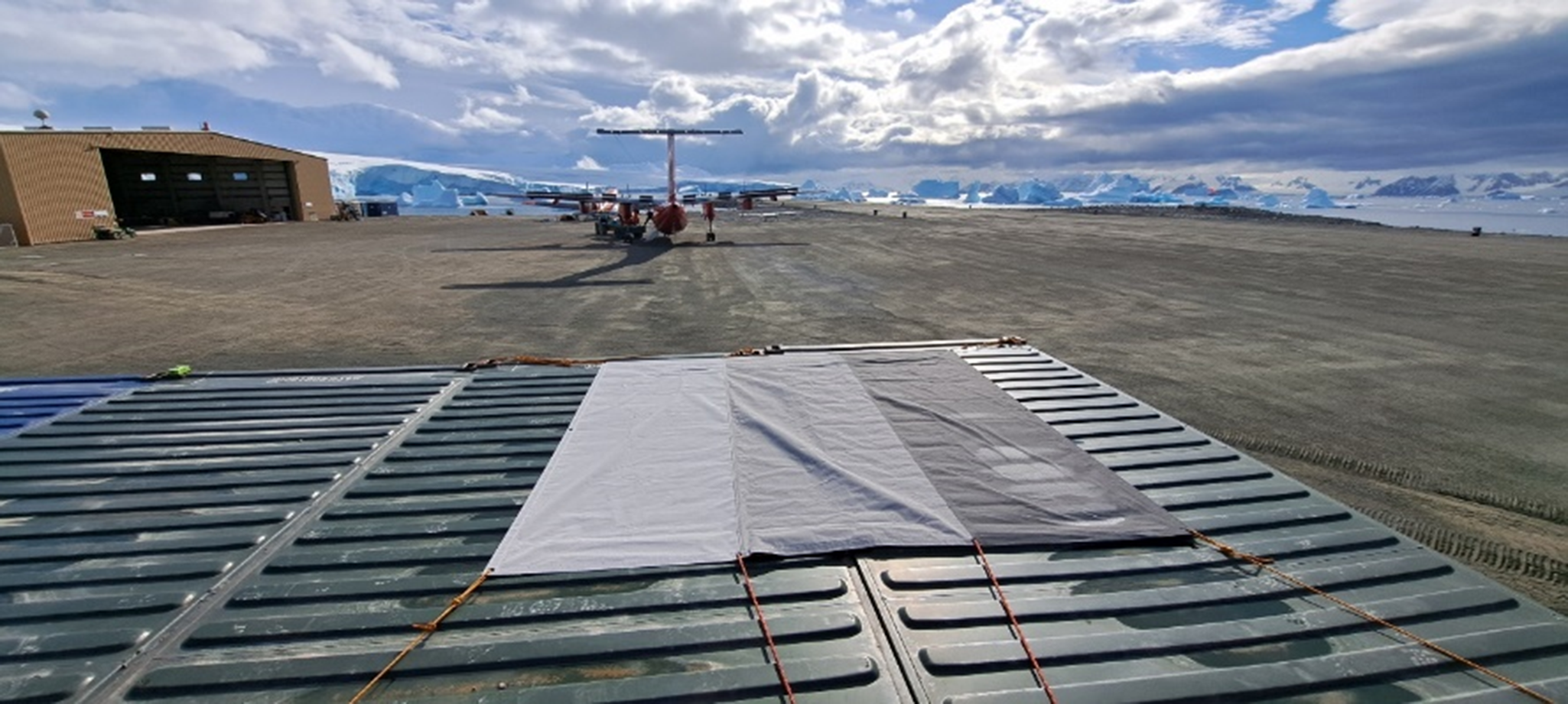
Figure 5. Hyperspectral calibration tarpaulin installed on top of shipping containers adjacent to the Rothera apron and runway.

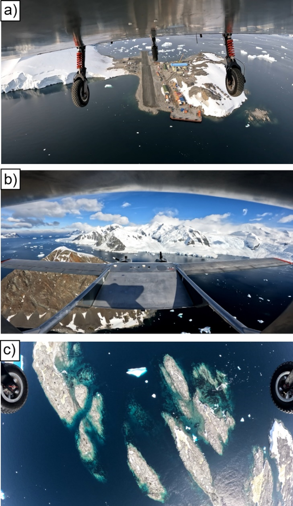
Figure 6. Stills from a. belly-mounted, b. tail-mounted and c. science floor-mounted GoPro cameras.

The second key sensor on the camera floor was the hyperspectral camera. Hyperspectral imagery records the full spectrum of observed light at every pixel in an image. This spectrum can be used to more accurately classify the material being observed. These data are primarily used for environmental and vegetation classification. However, depending in the frequencies observed, they can also be used to classify different rock types (Black et al. 2016) or water masses (Hartl et al. 2025), or potentially to identify the distribution of key marine animals such as krill (Belcher et al. 2021). To evaluate the utility of hyperspectral data collection from the Windracers Ultra, we flew a Headwall Nano HP visual and near-inferred (VNIR) hyperspectral imaging sensor. This uses a push-broom sensor to observe VNIR wavelength ranges of 400–1000 nm in 340 spectral bands across a 1020 pixel swath. As it is a push-broom sensor, the spectral image is built up as the sensor is moved through space. The sensor includes a Trimble Applanix inertial measurement unit (IMU) and GNSS receiver, which both provided real-time positional and attitude data and triggered data collection, as well as recording the GNSS/IMU data required for post-processing. The GNSS antenna used for the hyperspectral system was mounted approximately on the aircraft centreline.

For hyperspectral data collection, exposure time would ideally be relatively long to improve the signal to noise ratio across the spectral bands. However, to prevent blurring of pixels, longer exposure times can require platform speeds below the minimum speed of the Ultra (~28 m/s). The maximum permitted platform speed increases with survey platform altitude, but the ground pixel size also increases, decreasing the resolution of the data. A number of exposure rates and altitudes were used across the season. Flight S06 was flown at a relatively long 10 μs hyperspectral exposure, flights S07 to S09 used a 6 μs exposure, while flights S10–S12 used a 8 μs exposure. The spectral observations were initially calibrated by collection of a ‘dark reference’ (i.e. with the lens cap on) at the start of each flight, providing an estimate of system noise. Additional calibration for the prevailing atmospheric and lighting conditions and conversion to reflectance values were undertaken using a naturally illuminated 3 m × 3 m calibration tarpaulin (Fig. 5). This was overflown at the start and end of each flight, at the same altitude as the main survey flight. The calibration tarpaulin had three panels with uniform reflectance values of 11%, 30% and 56% and was placed on top of shipping containers adjacent to the Rothera apron/runway (Fig. 5). For initial processing, only the 56% reflectivity panel was used. Further processing included orthorectification using positional data from the Trimble Applanix IMU and GNSS receiver.

In addition to the dedicated high-specification camera systems, three GoPro cameras record data during each flight. Two of these cameras recorded 4K video: one mounted on the belly of the Ultra platform looking forward and the other mounted on the tail, also looking forward. These cameras provided the GCS operator with a retrospective look at flight conditions in terms of cloud cover and potential icing, building situational awareness across the season, as well as providing a valuable outreach and media resource (Fig. 6). One GoPro was mounted on each science floor, looking straight down, and it recorded a time lapse at one frame per second. This provided a quick view of the areas overflown and could potentially be used for future scientific analyses. The magnetic data-logging system (detailed in the ‘Gravity and magnetics’ section) was also installed on the camera floor, allowing collection of additional opportunistic data.

Camera flights were flown at an approximately constant height AGL. The maximum climb angle for the Windracers Ultra platform during BVLOS missions was 4°, limiting how precisely this ground clearance could be maintained. Where the terrain was too steep, it was planned that the minimum specified ground clearance was maintained over peaks but exceeded during the climb, ensuring that the observed swath width was always equal to or larger than expected. For flights S06–S09, a flight altitude of 450 m AGL was used. For flights S10–S12, a flight altitude of 500 m AGL was used. Over the sea, data were collected at a flight altitude of 500 m.

Post-processing of the photographic data showed that generation of mapping information of similar quality in terms of resolution and accuracy to that from the same camera system mounted on a Twin Otter is achievable (Fig. 7). Post-processing was carried out using Pix4D (version 4.9.0) software, which uses an advanced Structure from Motion (SfM) photogrammetry algorithm. Data collected by the onboard Javad GNSS receiver were processed against a base station using a post-processed kinematic (PPK) workflow to calculate the absolute position of each image centre. To achieve this, precise point positioning (PPP) processing was first undertaken on the data collected by the base station using the online Canadian Spatial Reference System Precise Point Positioning (CSRS-PPP) service (version 3). The PPK workflow was then undertaken within Trimble Business Center (version 2024.01), after which the processed solutions for each camera centre were exported. Once imported into Pix4D, the camera positions were updated with the PPK solutions, and tie points (common points between images) were generated both to further refine the geolocation of the images and to calculate the orientation of the camera during image acquisition. After image alignment was complete, a dense point cloud was extracted from the imagery and used to create a DEM of the surface within the survey area. The DEM was then used to create an orthorectified mosaic of the imagery. The output of this processing is a high-resolution DEM and orthorectified mosaic of the imagery with a resolution of 4.25 cm/pixel. Comparison with known tie points enables assessment of absolute horizontal and vertical error, giving an estimated root mean square (RMS) error for x, y and z of 0.405, 0.909 and 0.838 m, respectively. These relatively high errors are in part attributed to the use of the Javad GNSS data, which were referenced to an antenna offset ~75 cm from the camera centreline. Further post-processing using improved GNSS data and traditional photogrammetry (non-structure from motion-based solutions) will probably give improved performance.

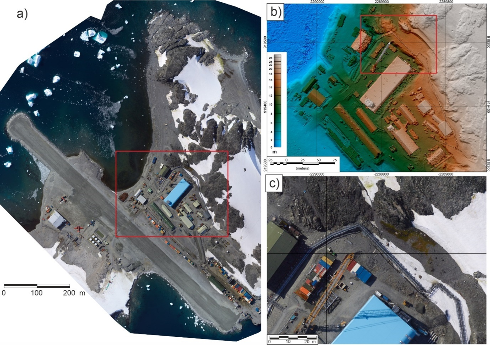
Figure 7. Orthophoto and digital elevation model (DEM) of Rothera Research Station. a. Full orthorectified mosaic. Red box locates b. b. Hill shade of DEM over Rothera Research Station buildings. Red box locates c. c. Detail of orthorectified mosaic. Note the brown/green area in upper right quadrant indicating a moss bank.

Given the slower speed of the Ultra relative to typical crewed aircraft, future missions may be flown closer to the ground, thereby enhancing resolution relative to data collection with the traditional Twin Otter platform, as pixel blur associated with rapid forward motion is reduced. We expect resolutions of 2 cm or better to be achievable at altitudes of ~225 m and/or using more advanced camera systems. The unmanned nature of the system did present some challenges. With no onboard operator or real-time remote control of the camera system, the camera exposure was controlled automatically by the camera system itself. However, the high-contrast nature of the environment (snow/ice and sea) is challenging for automatic exposure algorithms. Although it is possible to correct exposure during post-processing, this process remains largely manual and represents a significant amount of additional work. Moreover, while SfM photogrammetry is capable of overcoming some of the problems associated with datasets with limited exterior orientation information, it does necessitate significantly greater overlap between images, increasing both the time required to collect the data and any downstream data processing. The addition of an IMU integrated directly into the camera system in future would significantly improve both data collection and data processing efficiency.

Initial post-processing of the hyperspectral data was carried out using Hyperspec III (V3.3.1), a post-processing software package from Headwall Photonics. This confirmed that useful and valid spectral information was collected. The example of the initial quality control processing presented here used the real-time position and attitude solutions from the Trimble Applanix, coupled with the 2 m Reference Elevation Model of Antarctica (REMA) DEM (Howat et al. 2019) to orthorectify the imagery (Fig. 8a). For our preliminary test of the data quality, we applied a band-mixing technique to create a ‘false colour’ composite from the hyperspectral data (Fig. 8b). This approximately followed the standard Landsat 7 band 5, 4, 3 (near-infrared (NIR), red and green, respectively) mixing to generate an image in which vegetation is highlighted using strong red colours. Our results show that known areas of vegetation, such as the moss bank at Rothera Research Station (Convey & Smith 1997), can be readily identified (Fig. 8b), making this a useful technique to assess the other ASPAs we surveyed. The full VNIR spectrum holds additional information that can be used, for example, to discriminate between green snow algae and terrestrial plants (Fig. 8c).

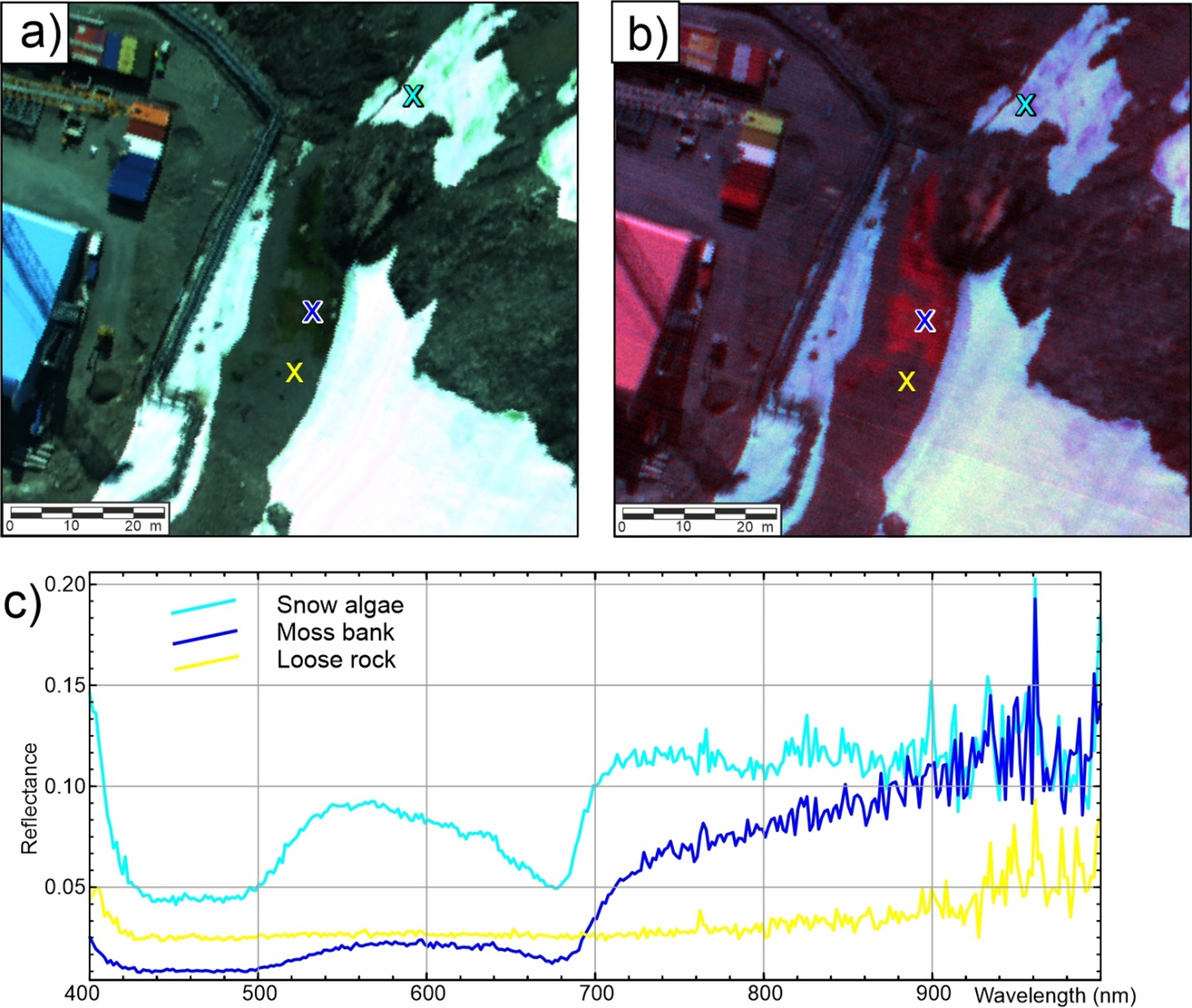
Figure 8. Example of orthorectified hyperspectral data over Rothera Research Station. a. Visual band (RGB) image centred on ‘bio gully’, a persistent moss bank (Convey & Smith 1997) also shown in Fig. 7c. Crosses locate points of spectral assessment shown in c. b. False-colour (near-infrared, red and green) spectral combination, highlighting vegetation using red colours. c. Observed reflected spectral patterns at three sample locations. Note the characteristic chlorophyll absorption at ~675 nm for moss and algae.

Atmospheric turbulence probe sensor

Atmospheric turbulence data provide crucial insights into, for example, the complex interactions and exchange processes between the ocean, sea ice and the atmosphere, enabling a deeper understanding of the mechanisms that drive polar weather systems (Renfrew et al. 2023). By analysing turbulence data, atmospheric processes can be better parameterized and predicted, helping us to understand how climate change may alter the interaction between the cryosphere, the ocean and the atmosphere. This can lead to more accurate forecasts of future weather patterns and their potential impacts on global and regional climates. From observing the three-dimensional turbulence components, the mean wind pattern (wind direction and wind speed) can be retrieved. Through the SWARM project, we tested the ability of a UAV to collect turbulence and wind data, with a view to future deployment of the probe for boundary-layer studies at lower altitudes in order to study the process of air-sea ice interaction and to collect such data with a BVLOS UAV, or even outside the normal Twin Otter operational window, such as during the winter, when Twin Otters are not present in Antarctica.

Atmospheric turbulence data were collected using an Aeroprobe 5-hole turbulence probe, with a Voyager data logger, including an integrated GNSS/INS unit. For this test, the probe was mounted on the port wingtip beside the aircraft peto-tube (Fig. 9). The probe, associated GNSS antenna, receiver, INS and data logger were all contained in a 3D-printed plastic housing, minimizing lever-arm considerations.

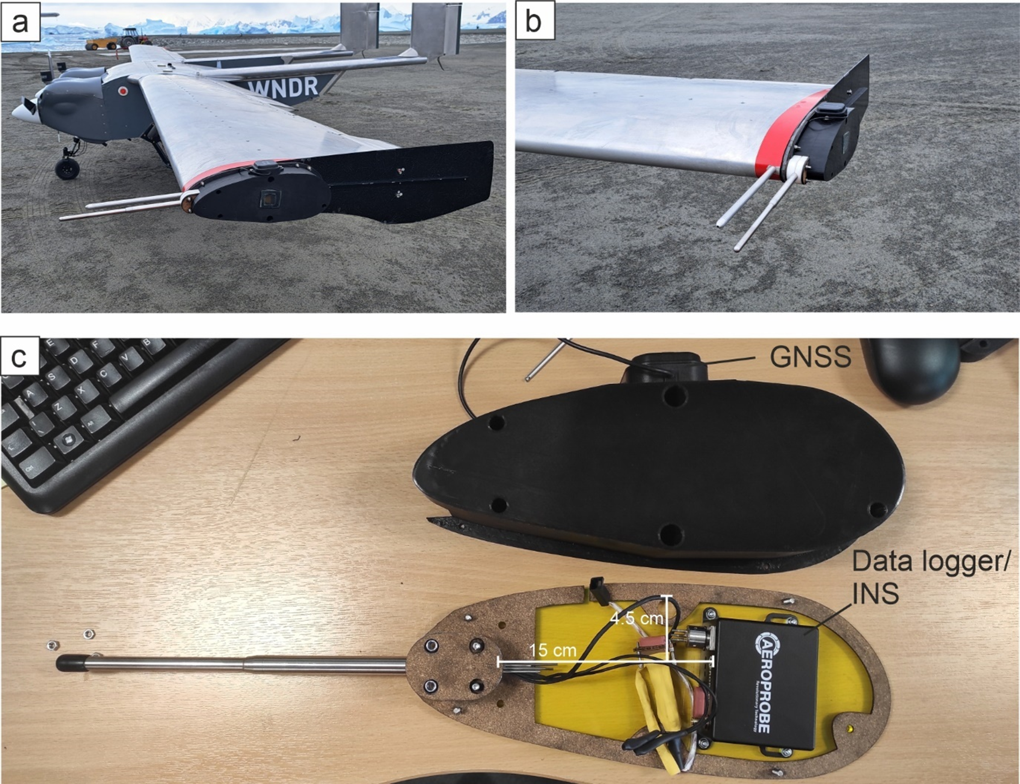
Figure 9. Aeroprobe 5-hole turbulence probe. a. Wing mounting location. b. Detail of wing mounting. c. Probe and data logger with housing removed. GNSS = Global Navigation Satellite System antenna. INS = Inertial Navigation System.

Two dedicated turbulence probe flights were flown to test the probe performance (Figs 4 & 10). S04 was a calibration flight, with two legs flown at a fixed altitude of 1000 m, 90° to each other (Fig. 10). S05 was a test mission profiling the atmosphere from 500 ft (~150 m) to 3000 ft (~1000 m). Subsequent flights also collected turbulence and wind data, providing a longer-term view on the performance of the sensor. The measured data include both the mean wind speed and the fluctuating components (turbulence). To provide a preliminary characterization of the turbulence probe data, we calculated the mean wind speed and direction on an L-shaped horizontal flight leg with perpendicular Ultra headings: out and return. The reported airspeed was converted into an East North Up (ENU) vector based on reported roll, pitch and yaw. The horizontal component of this was subtracted from the ENU velocity derived independently from the GNSS/INS solution to give the horizontal wind speed. Figure 10 shows the flight path of the calibration flight and the determined wind speed and direction derived from turbulence probe observations, corrected for aircraft motion. It is apparent that the values for wind speed and direction on the outbound and return legs match relatively well, indicating that the platform and system are collecting meaningful data.

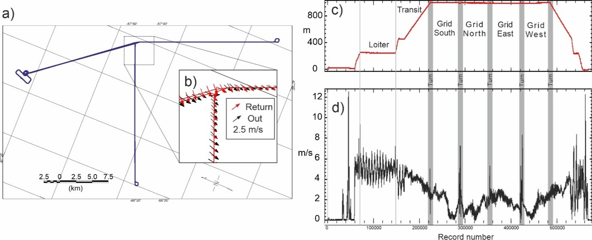
Figure 10. Preliminary results from the turbulence probe calibration flight. a. Map with flight path of calibration mission S04. Inset b. shows wind vector arrows for the outbound (black) and return (red) legs. Note the consistent recovered wind direction and amplitude on each leg, irrespective of flight direction. c. Flight profile showing survey elevation and stage of the mission. d. Recovered horizontal wind speed from differencing airspeed based on pressure and speed from the integrated Global Navigation Satellite System/Inertial Navigation System. Note that the zigzag pattern at the start of the flight reflects time in a circular loiter.

Gravity and magnetics

In Antarctica, airborne gravity and magnetic surveying are key techniques for assessing the subglacial geology and tectonic evolution of a region. Gravity data provide information regarding the density of subsurface materials, including water depth, different rock types and the thickness of the Earth’s crust. Magnetic data provide insights into the subsurface of a region due to the juxtaposition of rocks with different magnetic properties. Magnetic data are typically most informative about shallow structures, but they can also provide insights into more regional geology. To test the ability of the Ultra UAV to collect these datasets, we planned a 2 km line-spacing survey across a major tectonic discontinuity observed in the Antarctic Peninsula. Existing magnetic data indicated the location of the discontinuity but were of relatively low resolution, and airborne gravity data over this area consist of a single high-altitude (4.3 km) line.

Gravity data were collected using an iCORUS-02 strapdown gravity system hired from iMAR Ltd, which included a stabilized thermal enclosure (Fig. 11). The sensor was mounted on 2.5 cm vibration-damping shock mounts in the approximate centre of gravity of the aircraft, below the central GNSS antenna. The specific mounts were carefully chosen to supress the dominant disturbing frequency of the UAV (50 Hz or 3000 rpm). At this frequency, a static deflection in the mounts of 0.8 mm is required to dampen > 80% of the vibration. Given the load of the sensor on each mount (~34.4 N = 3.44 DaN), the stiffness of the shock mounts therefore had to be lower than 3.44/0.8 = 4.3 DaN/mm. A Fivistop M6 Anti Vibration Mount, with 15.5 kg compression load, 2025VD18-45, fulfilled this requirement.

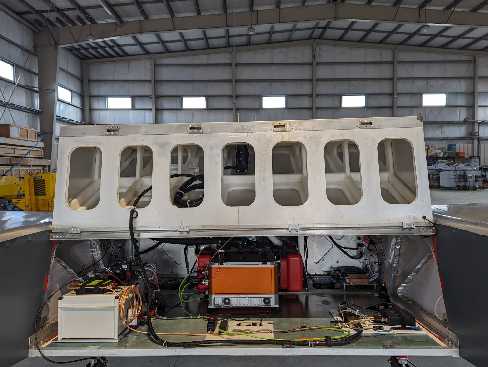
Figure 11. Gravity and magnetic floor. The grey box on the left is the power distribution. The orange box in the centre is the iMAR gravity system. The boxes on the right of the floor are the magnetometer system, including logger, fluxgate and inertial navigation system. The magnetometer sensor in the payload bay door is linked to the logger by the thick black cable. The cable in the lower left goes to the 28 V ground power supply used to maintain the iMAR system at temperature.

The gravity sensor was installed and powered 2 days prior to the gravity survey flights, allowing the internal temperature to stabilize, with a manually set ambient temperature of 5°C. This gave a permitted ambient operational temperature range of between −10 and +20°C, which was not exceeded. Note that the internal stabilized temperature of the system remains at a constant value, ~20°C above the set ambient value. The gravity system remained powered and at its stabilized temperature for the duration of the survey. The sensor was set to colect the required INS and GNSS data > 15 min prior to each survey flight, with static data also collected for > 15 min after each flight. GNSS base station data for post-processing were collected either at the Rothera International GNSS Service (IGS) station or using a tempoary Javad base station reciever installed adjacent to the runway.

Gravity values (referenced to the ellipsoid, so technically gravity disturbance) were calculated using the Terrapos GNSS processing software package. This implements a direct Kalman filtering approach to integrate INS data from accelerometer and gyroscope triads with GNSS satellite data to simultaneously solve for platform position and velocity as well as the gravitational field variations (Johann et al. 2019). To conduct the processing, precise satellite ephemeris were downloaded from the IGS to improve the quality of the solution. The behaviour of the Kalman filter can be adjusted based on the expected corelation (km) and standard deviation (mGal) of the gravity signal, with higher corelation and smaller standard deviation values acting to smooth the output signal. Tests showed that a filter with a correlation of 2 km and standard deviation of 10 mGal gave an output signal with relatively few apparent artefacts while maintaining the highest frequency of geological signals possible.

The lever-arm values between the gravity sensor and the GNSS antenna must also be known accurately for high-quality processing. These values were initially determined, with an accuracy of ~2 cm, by a combination of physical measurements and use of computer-aided design (CAD) images of the Windracers Ultra platform. Subsequently, the lever-arm estimate was improved by allowing the Kalman filter to optimize the lever-arm values. This procedure was applied to a magnetic compensation flight, as the relatively high dynamics (roll/pitch/yaw) give a better signal for solving the lever arm. After four iterations, stable, low-error (< 0.5 cm) lever-arm values were achieved, which were applied for all subsequent missions.

The output gravity values were visually assessed for quality using the Geosoft software package. Offsets between recovered gravity values for different flights of up to 20 mGal were apparent, with some flights showing an apparent linear trend of up to 5 mGal between start and end. To resolve this error, the output ‘absolute gravity’ value for the UAV during the static measurements before and after each flight was compared to the absolute gravity value reported for the Rothera Hanger tie point by René Forsberg during the PolarGAP survey (https://earth.esa.int/eogateway/documents/20142/37627/PolarGap-2015-2016-final-report.pdf). The differences were assumed to be the offset in the gravity anomaly value. A linear trend between the start and end static offsets was imposed to account for system/processing drift. All static readings were made within 50 m from the hanger tie point, and more typically within ~20 m, so this is a relatively robust check. Minor line-to-line offsets remained visible in the gravity data after levelling to the hanger tie point. Simple statistical levelling, applied using two missions flown either orthogonal or oblique to the main survey as tie lines, reduced the errors further. The southern part of the survey lacked tie lines, and an additional judgement was made to reduce the amount of statistical levelling in this region, as this provided the best visual minimization of line-to-line noise.

Figure 12. Free-air gravity anomaly maps. The black line marks the coast and grey lines are contours of the bathymetry from BEDMAP2. Note the good correspondence of the overall bathymetric pattern with the gravity signal. a. Initial free-air gravity values. b. Final free-air gravity anomaly map after base value correction and statistical levelling. Profile A-A’ locates Fig. 13.

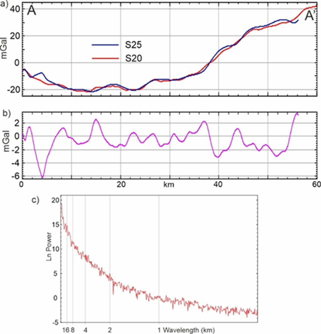
Figure 13. Example of overlapping gravity profiles along profile A-A’ in Fig. 12. a. Observed gravity anomaly. b. Difference between profiles. c. Average power spectra from six gravity flights - note that power rises above the noise floor at ~2 km wavelength.

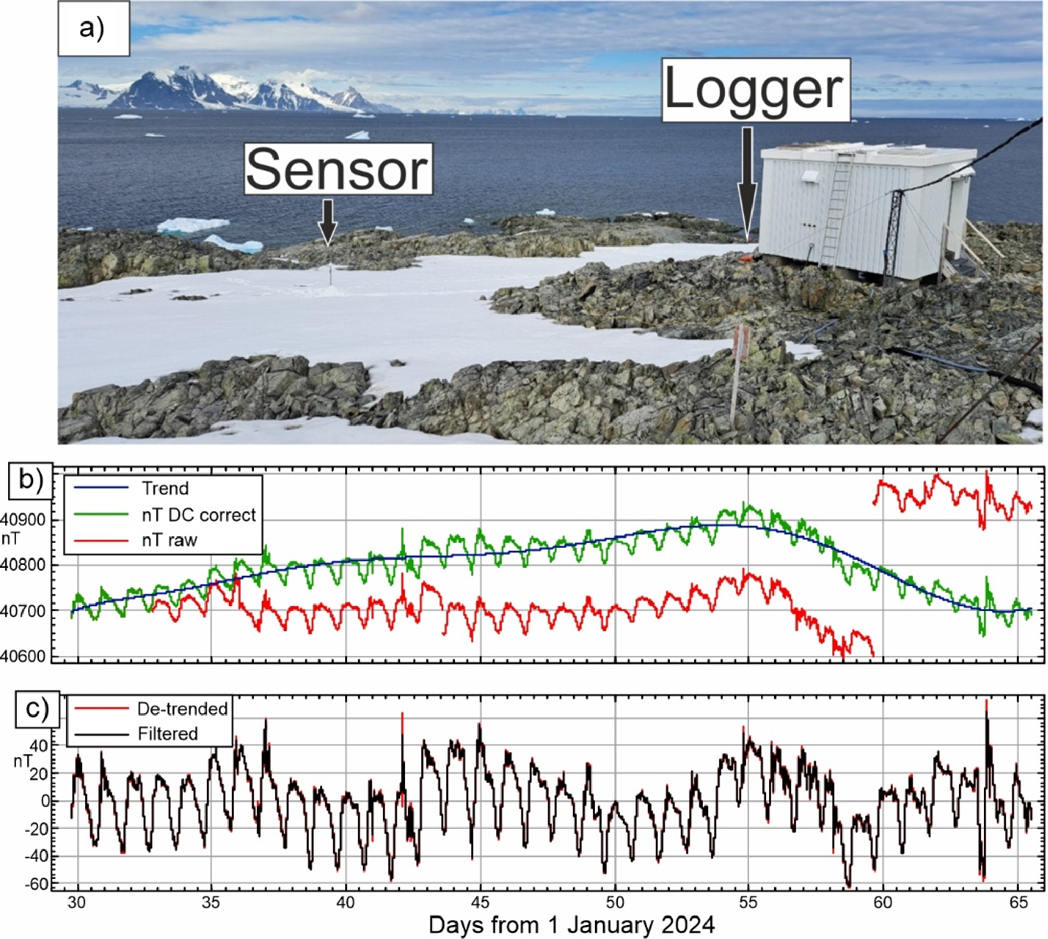
Figure 14. Magnetic base station and data. a. Temporary magnetic base station at optical hut on Rothera Point. b. Magnetic time series during operation (red), time series corrected for uniform offsets (green) and estimated trend (blue). c. De-trended magnetic time series (red) and 40 point mean filtered (10 min) times series (black).

To assess the quality of the data, we compared the gravity values from flights S20 and S25, which partially re-flew the same lines (Figs 12 & 13). After levelling, these profiles show a mean difference of −0.24 mGal and a standard deviation of 1.66 mGal. This standard deviation is taken as representative of the error across the wider survey area. To assess the minimum resolvable wavelength, we calculated the average power spectra of the gravity signal over six of the gravity flights (Fig. 13c). This shows that the spectral signal rises above the noise floor at ~2 km, which we take to be the minimum resolvable wavelength.

Airborne magnetic data were collected with a GEMSys GSMP-35U UAV magnetometer. Data were logged at 10 Hz and included GPS-derived time and position, total magnetic field (nT) as well as x, y and z fluxgate magnetometer information and roll, pitch and heading information from a small INS mounted on the aircraft floor (Fig. 11). To support the survey, a temporary magnetic base station was installed adjacent to the optical caboose on Rothera Point (Fig. 14). This recorded data at 15 s intervals using an Overhauser-type magnetometer. Data from this sensor were affected by long-term drift caused by progressive melting of the snow around the sensor support. Physically correcting this tilt created a number of abrupt uniform shifts in the recorded data. These uniform shifts were manually adjusted before an eighth-order polynomial was fit across the full 36 days of data to remove residual long-term trends. Finally, the base station data were filtered with a 40 point mean filter (10 min) to remove high-frequency noise that may not be seen in the airborne data (Fig. 14b,c). This filtered and de-trended data formed the magnetic base station correction. The magnetic base station showed a generally stable diurnal trend on each day (Figs 14 & 15). Most flights were flown between 12h00 and 18h00 UTC, avoiding the magnetically noisy period between 18h00 and 06h00 UTC (Fig. 15).

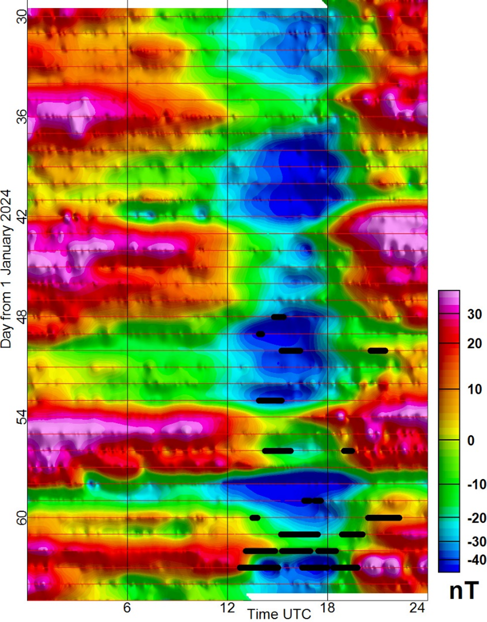
Figure 15. Magnetic base station data as date vs time plot; amplitude is the base station correction. Data were de-trended with a polynomial to account for long-wavelength trends. Thin red lines indicate base station operation. Thick black lines mark survey flights including the magnetometer system.

The first stage in the processing of the airborne magnetic data was the manual removal of spikes and noisy turn manoeuvres. Subsequently, the 10 Hz data were filtered with a 10 point mean filter (1 s) to suppress residual high-frequency noise attributed to the mounting of the sensor relatively close to engines, power systems and electronic control surfaces. To compensate for magnetic fields induced by dynamic movement of the aircraft, a compensation/calibration flight was conducted. Typically, this is done at high altitude (> 10 000 ft) in a magnetically quiet area. However, to induce the required manoeuvres we used the safety pilot controls to ‘nudge’ the platform. The compensation flight was therefore conducted as a VLOS mission at an altitude of 1000 ft around Rothera. This placed the compensation flight over a long-wavelength (~3 km), relatively high-amplitude (~300 nT) anomaly. This is not an ideal setting; however, the long wavelength of the background anomaly meant that the shorter-wavelength signatures of the compensation manoeuvres remained distinct. The compensation mission was flown in a repeated clover-leaf shape. Each repetition of the clover leaf tested a specific manoeuvre in each of the survey directions (i.e. roll: N, W, S and E; then pitch: N, W, S and E; then yaw: N, W, S and E). This procedure was flown over two distinct flights ~20 min apart due to intermittent low cloud. Magnetic compensation coefficients were calculated using the Aeromagnetic Compensation Postprocessing Application from GEMSystems to solve the system of equations describing the field associated with a moving aircraft (Leliak 1961). Prior to magnetic compensation, the fluxgate data were de-spiked using a non-linear filter with width of 1 and a tolerance of 1000, and the data were also filtered with a 10 point mean filter (1 s) consistent with the filter applied to the total field data. Compensation provided a reduction in the standard deviation of the filtered compensation data from 41.6 nT pre-compensation to 6.3 nT post-compensation. The calculated coefficients were then applied to the entire survey.

After compensation, the global reference field calculated using the 2020 International Geomagnetic Reference Field (IGRF) model, implemented in the Geosoft Oasis montaj program, was subtracted from the compensated total field values. The time, position (longitude, latitude) and flight elevation of the aircraft were used to estimate the total field. After removal of the global reference field, the base station correction was subtracted to remove diurnal variations in the magnetic field (Figs 15 & 16a).

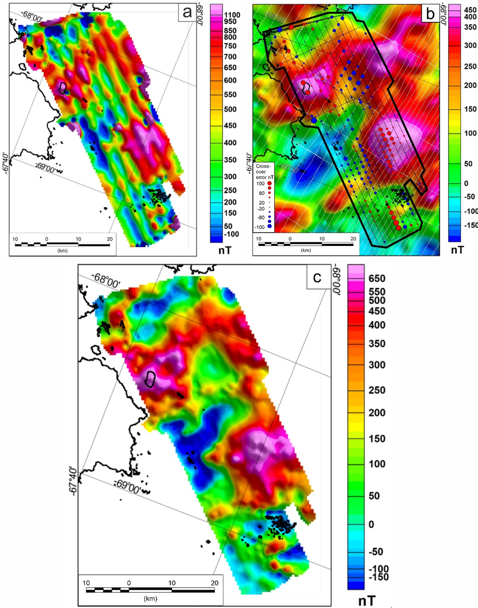
Figure 16. SWARM magnetic survey data. a. Raw magnetic data with the International Geomagnetic Reference Field (IGRF) total field value removed. Note the significant line-to-line noise. b. ADMAP-2 magnetic data used as reference for levelling. The black outline shows the SWARM survey area. The thin black lines show the SWARM flight lines. The thin white lines are from the ADMAP-2 data. Note the largest residual cross-over errors between the ADMAP-2 and SWARM data associated with the highest-amplitude anomalies (red or blue circles indicate SWARM values being above or below ADMAP-2 values, respectively). c. Final post-processed and levelled SWARM magnetic product. Note the improvement in resolution relative to ADMAP-2 data due to the lower flight altitude.

The final stage of processing applied to the magnetic data was levelling. The SWARM data were levelled against pre-existing ADMAP-2 data (Fig. 16b), which was flown almost perpendicular to the SWARM survey, providing a large number of tie line crossings. However, the ADMAP-2 line data were collected been 2440 and 1220 m altitude and show much reduced amplitude and resolution compared to the SWARM data collected at a target altitude of 500 m. To perform the levelling, the SWARM line data and lower-altitude ADMAP-2 data were both upward continued to the maximum altitude of 2440 m. The SWARM data were also split into data segments with constant flight headings. Cross-over analysis and statistical levelling were then applied to the SWARM data, typically removing either zero- or first-order polynomial trends. During the levelling process, it was initially assumed that the ADMAP-2 data were generally robust. Levelling was applied iteratively, with large outliers removed at each stage. A systematic correlation of residual errors between the ADMAP-2 and SWARM data became apparent after initial levelling, with higher-amplitude positive and negative anomalies being underestimated in the ADMAP-2 data (Fig. 16b). We attribute this to differences in the pre-processing and continuation of the original survey data from ADMAP-2, and we did not minimize the offset in the SWARM data with higher-order polynomial trends. The low-order polynomial levelling process was iterated until a satisfactory result was achieved, defined as no obvious artefacts in the flight-line direction when gridding the levelled SWARM data. This was a well-levelled product, but it showed a significant degradation in resolution due to upward continuation. The levelled magnetic product was therefore subtracted from the upward continued SWARM line data to obtain the levelling correction. This long-wavelength levelling correction, typically a DC shift or linear trend, was then added to the SWARM line data at the original altitude. This procedure levelled the SWARM data against the ADMAP-2 data while retaining the higher resolution achieved by the significantly lower-altitude survey (Fig. 16c).

Discussion

This field season demonstrated that the Windracers Ultra UAV can successfully collect meaningful amounts of Antarctic environmental scientific data on regional missions lasting several hours and covering hundreds of kilometres. Operation of the Ultra went smoothly, with communication and integration with standard Rothera operations proving relatively simple. Specifically, we were able to demonstrate that communication between crewed aircraft and the GCS operator could be easily managed over the radio via the Rothera tower coordinator, paving the way for future integrated operations. During the season, it was also demonstrated that a remote GCS operator, based in Southampton, could successfully control the Ultra using the Distributed Avionics Cloud Control system. For this demonstration, a Starlink satellite communication system was installed. The aircraft was launched as normal from Rothera; however, during the flight, operators at the Windracers base in Southampton were able to log into the Distributed Avionics Cloud Control system and re-task the platform. The Rothera GCS operator maintained an observational role and was ready to take over in case of any change in operational conditions indicated by the Rothera tower, but control by a remote GCS pilot was demonstrated. Such remote operation has obvious advantages in terms of reducing the number of people required in the field to support future operations. However, it was found that having the GCS operator in Rothera significantly improved their situational awareness and was a major factor in facilitating air integration. In addition, protocols for communications between a remote GCS operator and the Rothera tower would need to be developed, building on those used this season. In the short to medium term, operations with UAV platforms such as the Windracers Ultra are therefore likely to benefit from an on-site GCS operator, especially when other aircraft are active. Across the season, during routine operations, the safety pilot only took control to complete three landings to maintain their operational currency/certification. As confidence grows in the Ultra platform and the auto-landing system is demonstrated to be robust over hundreds to thousands of landings, it may be advantageous to replace the safety pilot with personnel with a more general skillset, who could simply manage ground handling/taxiing of the aircraft, in communication with the GCS operator.

As a physical science platform, the Ultra performed well. The payload capability of the platform proved adequate for the installed equipment (up to ~45 kg), and no trade-off had to be made between range and payload for the planned missions. The Ultra was able to provide power for all of the scientific equipment in flight. The inclusion of a 24 V battery was a useful addition, allowing seamless transfer of the platform between the science team setting up equipment and downloading data and the operational flight crew, thereby streamlining operations. It also improved the safety factor of the operation, as there was no need for non-aircrew to interact with the platform while the engines were powered. However, the battery accounted for a significant proportion of the payload (15.8 kg), and use of a smaller battery, potentially coupled with an effective ground power source, could maximize the payload available for science in future seasons. Across the season, we typically flew one or two missions per day, with the main constraint being the weather factor impacting the collection of hyperspectral data. However, collection of 500–600 km of data per day (three missions) was a comfortable operational rate, allowing us to take advantage of the good weather window at the end of the season (Fig. 3).

We had planned to test fly an ice-penetrating radar during this field deployment. Unfortunately, during ground testing, it was shown that the radar interfered with a specific prototype component of the UAV communications system. Further ground testing showed that improved electromagnetic interference (EMI) shielding of this component rectified the problem, and this will be incorporated as an update to the Ultra platform. However, there was insufficient time during the season to fully and robustly implement this solution, so no airborne radar data were collected.

One constraint on the operational envelope of the Ultra that became apparent across the field season was the lack of on-board icing detection/mitigation. Our mitigation strategy was therefore to avoiding flying in cloud, as all clouds in the region had a reasonably high icing potential, given the expected local temperatures of ~0°C ± 10°C. This consideration limited our operational window to periods when forecasts, satellite images and local observations indicated few or no clouds at survey altitude. In addition, elevated in-flight relative humidity transmitted to the GCS by the UAV was taken as a proxy for cloud and hence as a trigger for considering aborting the mission due to suspected icing conditions. In the short to medium term, including icing detection would significantly increase the operational window, as it would allow the platform to continue a mission until icing was detected rather than aborting a mission simply based on a suspicion of significant cloud that may or may not generate icing. In future, icing mitigation measures would further extend the operational window. Such measures will become especially relevant when operating over long survey missions during which weather conditions might change.

A second constraint on operations was the fact that the specific Ultra platform relied on a radio link for communication with the GCS. Topography, which is quite extreme in the Rothera region, generated significant but predictable local radio shadows. Flying into these regions meant communications were lost for periods of between 2 and 16 min. As these radio shadows were predictable, an operational checklist was performed ~5 min before communication was lost, ensuring UAV system health was 100% and optimum flying conditions were present (low wind, low humidity, good satellite image and good weather forecast). A robust satellite communication system would alleviate this issue, allowing missions to continue into areas of radio shadow even if flying conditions were not totally optimal, further expanding the operational envelope of the platform. Such a communication system, independent of any line-of-sight considerations, would also become important for missions extending > 100 km from the operational base. During this season, we demonstrated the use of a Starlink satellite communications system; however, this will require further design work to reduce the weight and power consumption in order to make it compatible with the collection of scientific data using the Ultra platform.

This field season has demonstrated that the Ultra can fly from an Antarctic station with a gravel runway, using ~270 m length of runway for take-offs and landings. It is noted that no specific consideration was made to minimize the length of runway used, as ~900 m was available. The Ultra has been demonstrated to take off and land on runways as short as 150 m; hence, more optimized landing patterns could reduce the length of runway required if, for example, operating from short, temporary landing strips on remote sub-Antarctic islands. In future, operating the Ultra platform from snow/ice runways will be necessary if it is to be utilized towards central Antarctica. This could be achieved with the Ultra in its current wheeled configuration if ground equipment and snow conditions allowed grooming of a compacted runway. Alternatively, equipping the platform with skis would be a technical possibility. However, studies are required to assess the extent to which this might compromise the total range/available payload. Logistical advantages in terms of the reduction of field fuel used by survey aircraft will not be fully realized until this issue is addressed.

Conclusions

Our field season has demonstrated that large UAVs such as the Windracers Ultra are viable platforms for the collection of Antarctic environmental scientific data over ranges of hundreds of kilometres, representing a significant step towards their routine use. Good communications and the potential for close operational coordination with other aircraft pave the way for integrated operations going forward. This is critical if the potential of large UAVs for scientific data collection in Antarctica is to be realized.

During this season, we demonstrated that visual camera, hyperspectral, gravity, magnetic, turbulence and wind data can all be collected with the Ultra UAV in a similar manner to a traditional platform, showing promising results. In some cases, such as for the hyperspectral data, the slower flying speed of the Ultra represented a direct benefit to the quality of the data collected. We aimed to demonstrate during this season the utility of the Windracers Ultra for gathering environmental data in Antarctica. However, these types of datasets also have significant use for environmental monitoring and mapping outside Antarctica. This study therefore demonstrates the utility of the Windracers Ultra as a platform for environmental scientific applications around the world.

Although the season was very successful and the Ultra can be considered proven for basic Antarctic operations from research stations, a number of operational challenges have been identified. These include icing detection/mitigation, robust satellite communication and the ability to operate from ice and snow. Adding these features represents the next step towards making Antarctic data collection from large UAVs routine.