


1. Introduction
Distributions with infinite mean are ubiquitous in the realm of banking and insurance, and they are particularly useful in modeling catastrophic losses (Ibragimov et al., Reference Ibragimov, Jaffee and Walden2009), operational losses (Moscadelli, Reference Moscadelli2004), costs of cyber risk events (Eling and Wirfs, Reference Eling and Wirfs2019), and financial returns from technology innovations (Silverberg and Verspagen, Reference Silverberg and Verspagen2007); see also Chen and Wang (Reference Chen and Wang2025) for a list of empirical examples of distributions with infinite mean.
As the world is arguably finite (e.g., any loss is bounded by the total wealth in the world), why should we use models with infinite mean as mathematical tools? The main reason is that infinite-mean models often fit extremely heavy-tailed datasets better than finite-mean models. Moreover, the sample mean of iid samples of heavy-tailed data may not converge or may even tend to infinity as the sample size increases. Therefore, it is not sufficient to conclude that infinite-mean models are unrealistic by the finiteness of the sample mean. Indeed, models with infinite moments are not “improper” as emphasized by Mandelbrot (Reference Mandelbrot1997), and they have been extensively used in the financial and economic literature (see Mandelbrot, Reference Mandelbrot1997 and Cont, Reference Cont2001).
This paper focuses on establishing some stochastic dominance relations for infinite-mean models. For two random variables X and Y, X is said to be smaller than Y in stochastic order, denoted by $X \le_\textrm{st } Y$
, if
$X \le_\textrm{st } Y$
, if $\mathbb{P}(X \le x) \ge \mathbb{P}(Y\le x)$
for all
$\mathbb{P}(X \le x) \ge \mathbb{P}(Y\le x)$
for all $x \in \mathbb{R}$
; see Müller and Stoyan (Reference Müller and Stoyan2002) and Shaked and Shanthikumar (Reference Shaked and Shanthikumar2007) for extensive accounts of properties of stochastic dominance. Let X be a positive one-sided stable random variable with infinite mean and
$x \in \mathbb{R}$
; see Müller and Stoyan (Reference Müller and Stoyan2002) and Shaked and Shanthikumar (Reference Shaked and Shanthikumar2007) for extensive accounts of properties of stochastic dominance. Let X be a positive one-sided stable random variable with infinite mean and $X_{1},\dots,X_{n}$
be iid copies of X. For a nonnegative vector
$X_{1},\dots,X_{n}$
be iid copies of X. For a nonnegative vector $\left(\theta_{1},\dots,\theta_n\right)$
with
$\left(\theta_{1},\dots,\theta_n\right)$
with $\sum_{i=1}^n\theta_i=1$
, Ibragimov (Reference Ibragimov2005) showed that
$\sum_{i=1}^n\theta_i=1$
, Ibragimov (Reference Ibragimov2005) showed that
 \begin{equation} X\le_\textrm{st}\theta_{1}X_{1}+\dots+\theta_{n}X_{n}.\end{equation}
Recently, Arab et al. (Reference Arab, Lando and Oliveira2024), Chen et al.(Reference Chen, Embrechts and Wang2025a), and Müller (2024) have shown that inequality (1.1) holds for more general classes of distributions. The case of two Pareto random variables with tail parameter 1/2 was studied in Example 7 of Embrechts et al. (Reference Embrechts, McNeil and Straumann2002); see Section 3 for the precise definition of the Pareto distribution.
Inequality (1.1) provides very strong implications in decision-making as it surprisingly holds in the strongest form of risk comparison. If $X_1,\dots,X_n$
are treated as losses in a portfolio selection problem, any agent who prefers less loss will choose to take one of
$X_1,\dots,X_n$
are treated as losses in a portfolio selection problem, any agent who prefers less loss will choose to take one of $X_1,\dots,X_n$
instead of allocating their risk exposure over different losses. This observation is counterintuitive, contrasting with the common belief that diversification reduces risk. Other applications of (1.1) include optimal bundling problems (Ibragimov and Walden, Reference Ibragimov and Walden2010) and risk sharing (Chen et al., Reference Chen, Embrechts and Wang2024).
$X_1,\dots,X_n$
instead of allocating their risk exposure over different losses. This observation is counterintuitive, contrasting with the common belief that diversification reduces risk. Other applications of (1.1) include optimal bundling problems (Ibragimov and Walden, Reference Ibragimov and Walden2010) and risk sharing (Chen et al., Reference Chen, Embrechts and Wang2024).
In this paper, we will study (1.1) where $X_1,\dots,X_n$
are possibly negatively dependent, a case not considered in Ibragimov (Reference Ibragimov2005), Arab et al. (Reference Arab, Lando and Oliveira2024), and Müller (2024). Chen et al.(Reference Chen, Embrechts and Wang2025a) have shown that (1.1) also holds for weakly negatively associated super-Pareto random variables
$X_1,\dots,X_n$
are possibly negatively dependent, a case not considered in Ibragimov (Reference Ibragimov2005), Arab et al. (Reference Arab, Lando and Oliveira2024), and Müller (2024). Chen et al.(Reference Chen, Embrechts and Wang2025a) have shown that (1.1) also holds for weakly negatively associated super-Pareto random variables $X_{1},\dots,X_{n}$
. The class of super-Pareto random variables is quite broad and can be obtained by applying increasing and convex transforms to a Pareto random variable with tail parameter 1. Examples of super-Pareto distributions include the Pareto, generalized Pareto, Burr, paralogistic, and log-logistic distributions, all with infinite mean.
$X_{1},\dots,X_{n}$
. The class of super-Pareto random variables is quite broad and can be obtained by applying increasing and convex transforms to a Pareto random variable with tail parameter 1. Examples of super-Pareto distributions include the Pareto, generalized Pareto, Burr, paralogistic, and log-logistic distributions, all with infinite mean.
This paper aims to further generalize the result of Chen et al. (Reference Chen, Embrechts and Wang2025a) in two aspects: the marginal distribution and the dependence structure of $(X_{1},\dots,X_{n})$
. In Section 3, we first introduce a new class of distributions, which has several nice properties (Propositions 2 and 3) and includes the class of super-Pareto distributions as a special case. Within this class of distributions, we show in Theorem 1 that (1.1) holds for identically distributed random variables
$(X_{1},\dots,X_{n})$
. In Section 3, we first introduce a new class of distributions, which has several nice properties (Propositions 2 and 3) and includes the class of super-Pareto distributions as a special case. Within this class of distributions, we show in Theorem 1 that (1.1) holds for identically distributed random variables $X_1,\dots,X_n$
that are negatively lower orthant dependent (Block et al., Reference Block, Savits and Shaked1982). It is well known that the behavior of the sum of extremely heavy-tailed random variables is dominated by the maximum of the summands (see Embrechts et al., Reference Embrechts, Klüppelberg and Mikosch1997). Therefore, a possible reason why (1.1) is preserved when transitioning from independence to negative dependence is because under negative dependence, random variables that take small to moderate values will push the other random variables to take large values with a larger probability, leading to a stochastically larger
$X_1,\dots,X_n$
that are negatively lower orthant dependent (Block et al., Reference Block, Savits and Shaked1982). It is well known that the behavior of the sum of extremely heavy-tailed random variables is dominated by the maximum of the summands (see Embrechts et al., Reference Embrechts, Klüppelberg and Mikosch1997). Therefore, a possible reason why (1.1) is preserved when transitioning from independence to negative dependence is because under negative dependence, random variables that take small to moderate values will push the other random variables to take large values with a larger probability, leading to a stochastically larger $\sum_{i=1}^n\theta_iX_i$
. The situation is different for positively dependent random variables; see Remark 5. As negative lower orthant dependence is more general than weak negative association, Theorem 1 (i) of Chen et al. (Reference Chen, Embrechts and Wang2025a) is implied by Theorem 1. Remarkably, while Theorem 1 is more general, it is shown by a much more concise proof.
$\sum_{i=1}^n\theta_iX_i$
. The situation is different for positively dependent random variables; see Remark 5. As negative lower orthant dependence is more general than weak negative association, Theorem 1 (i) of Chen et al. (Reference Chen, Embrechts and Wang2025a) is implied by Theorem 1. Remarkably, while Theorem 1 is more general, it is shown by a much more concise proof.
In Section 4, we proceed to study (1.1) given non-identically distributed random variables $X_1,\dots,X_n$
. Since
$X_1,\dots,X_n$
. Since $X_1,\dots,X_n$
do not follow the same distribution, the choice of X becomes unclear. A possible choice is to let X follow the generalized mean of the distributions of
$X_1,\dots,X_n$
do not follow the same distribution, the choice of X becomes unclear. A possible choice is to let X follow the generalized mean of the distributions of $X_1,\dots,X_n$
. A special case is the arithmetic mean, which leads to the commonly used distribution mixture models. Considering a rather large class of distributions, Theorem 2 shows that (1.1) holds if the distribution of X is the generalized mean with non-negative power of the distributions of
$X_1,\dots,X_n$
. A special case is the arithmetic mean, which leads to the commonly used distribution mixture models. Considering a rather large class of distributions, Theorem 2 shows that (1.1) holds if the distribution of X is the generalized mean with non-negative power of the distributions of $X_1,\dots,X_n$
. To our best knowledge, Theorem 2 is the first attempt to establish a nontrivial version of (1.1) for non-identically distributed random variables.
$X_1,\dots,X_n$
. To our best knowledge, Theorem 2 is the first attempt to establish a nontrivial version of (1.1) for non-identically distributed random variables.
The rest of the paper is organized as follows. In Section 2, we present some first observations on (1.1). Sections 3 and 4 present the main results. Section 5 compares our results with the literature. Section 6 concludes the paper. The appendix contains the proofs of Propositions 2 and 3 as well as some examples in the new class of distributions.
1.1 Notation, conventions, and definitions
In this section, we collect some notation and conventions used throughout the rest of the paper and remind the reader of some well-known definitions.
A function f on $(0,\infty)$
is said to be subadditive if
$(0,\infty)$
is said to be subadditive if $f(x+y)\le f(x)+f(y)$
for any
$f(x+y)\le f(x)+f(y)$
for any $x,y\gt0$
. If the inequality is strict, we say f is strictly subadditive. For a random variable
$x,y\gt0$
. If the inequality is strict, we say f is strictly subadditive. For a random variable $X\sim F$
, denote by
$X\sim F$
, denote by $\textrm{ess{-}inf}\ X$
(
$\textrm{ess{-}inf}\ X$
( $\textrm{ess{-}inf}\ F$
) and
$\textrm{ess{-}inf}\ F$
) and $\textrm{ess{-}sup}\ X$
(
$\textrm{ess{-}sup}\ X$
( $\textrm{ess{-}sup}\ F$
) its essential infimum and essential supremum. Denote by
$\textrm{ess{-}sup}\ F$
) its essential infimum and essential supremum. Denote by $\Delta_n$
the standard simplex, that is,
$\Delta_n$
the standard simplex, that is, $\Delta_n=\{\bar{\theta} \in [0,1]^n: \sum_{i=1}^n \theta_i=1\}$
, where we use notation
$\Delta_n=\{\bar{\theta} \in [0,1]^n: \sum_{i=1}^n \theta_i=1\}$
, where we use notation $\bar{\theta}$
for a vector
$\bar{\theta}$
for a vector $(\theta_1,\dots,\theta_n)$
. Let
$(\theta_1,\dots,\theta_n)$
. Let $\Delta_n^+=\Delta_n\cap (0,1)^n$
. We will also use [n] to denote the set of indices
$\Delta_n^+=\Delta_n\cap (0,1)^n$
. We will also use [n] to denote the set of indices $1,\dots,n$
. For a distribution function F, its generalized inverse is defined as
$1,\dots,n$
. For a distribution function F, its generalized inverse is defined as
 \begin{align*}F^{-1}(p)=\inf\{t\in\mathbb{R}\,:\,F(t)\geq p\}, p\in(0,1).\end{align*}
Definition 1. We say that a random variable X is smaller than a random variable Y in stochastic order, denoted by $X \le_\textrm{st } Y$
, if
$X \le_\textrm{st } Y$
, if $\mathbb{P}(X \le x) \ge \mathbb{P}(Y\le x)$
for all
$\mathbb{P}(X \le x) \ge \mathbb{P}(Y\le x)$
for all $x \in \mathbb{R}$
. For random variables X and Y with support
$x \in \mathbb{R}$
. For random variables X and Y with support $[c,\infty)$
where
$[c,\infty)$
where $c\in\mathbb{R}$
, we write
$c\in\mathbb{R}$
, we write $X\lt _{\rm st}Y$
if
$X\lt _{\rm st}Y$
if $\mathbb{P}(X\le x)\gt \mathbb{P}(Y\le x)$
for all
$\mathbb{P}(X\le x)\gt \mathbb{P}(Y\le x)$
for all $x\gt c$
.
$x\gt c$
.
2. Some observations on the stochastic dominance
Throughout the paper, we work with random variables that are almost surely nonnegative.
The main focus of the paper is on studying random variables X such that
 \begin{equation} X \le_\textrm{st} \theta_1 X_1 + \dots + \theta_n X_n\ \mbox{for all $\bar{\theta} \in \Delta_n$,}\end{equation}
where $X_1, \dots, X_n$
are independent or negatively dependent with the marginal laws equal to X (see Section 3.2 for the precise definition of negative dependence). We will also say that a distribution F satisfies property (SD) if a random variable
$X_1, \dots, X_n$
are independent or negatively dependent with the marginal laws equal to X (see Section 3.2 for the precise definition of negative dependence). We will also say that a distribution F satisfies property (SD) if a random variable $X\sim F$
satisfies it. If some of
$X\sim F$
satisfies it. If some of $\theta_1,\dots,\theta_n$
are 0, we can simply reduce the dimension of our problem. Therefore, for most of our results, we will assume
$\theta_1,\dots,\theta_n$
are 0, we can simply reduce the dimension of our problem. Therefore, for most of our results, we will assume $\bar{\theta}\in\Delta_n^+$
.
$\bar{\theta}\in\Delta_n^+$
.
Since (SD) holds if a constant is added to X, we will, without loss of generality, only consider random variables with essential infimum 0. We will also be interested in distributions, and random variables, for which property (SD) holds with a strict inequality. Let us start by formulating and providing some straightforward observations of (SD).
Proposition 1. Assume that random variables X and Y satisfy property (SD) and are independent. Then the following statements hold.
-
(i) $\mathbb{E}(X) = \infty$
or X is a constant.
$\mathbb{E}(X) = \infty$
or X is a constant. -
(ii) A random variable
$aX + b$
with
$a \ge 0$
and
$b \in \mathbb{R}$
satisfies (SD). -
(iii) Random variables
$\max\{X,c\}$
and
$\max\{X,Y\}$
satisfy (SD), with
$c \ge 0$
. -
(iv) A random variable g(X) with a convex nondecreasing function g satisfies (SD). In addition, if X satisfies (SD) with a strict inequality, g is convex and strictly increasing, then g(X) also satisfies (SD) with a strict inequality.


Proof.
-
(i) This is implied by Proposition 2 of Chen et al. (Reference Chen, Embrechts and Wang2025a).
-
(ii) The proof is straightforward and is omitted.
-
(iii) We will prove only the stronger property for the maximum of two random variables. Let
$X_{1},\dots,X_{n}$
follow the distribution of X,
$Y_{1},\dots,Y_{n}$
follow the distribution of Y, and
$\{X_i\}_{i\in[n]}$
and
$\{Y_i\}_{i\in[n]}$
be independent. For
$x\in\mathbb{R}$
and
$\bar \theta\in\Delta_n$
, we have
\begin{align*}\mathbb{P}(\!\max\{X,Y\} \le x) & = \mathbb{P}(X\le x) \mathbb{P}(Y\le x) \ge \mathbb{P}\left(\sum_{i=1}^n \theta_i X_i \le x\right) \mathbb{P}\left(\sum_{i=1}^n \theta_i Y_i \le x\right)\\& = \mathbb{P}\left(\sum_{i=1}^n \theta_i X_i \le x, \sum_{i=1}^n \theta_i Y_i \le x\right) = \mathbb{P}\left(\max\left\{\sum_{i=1}^n \theta_i X_i, \sum_{i=1}^n \theta_i Y_i\right\} \le x\right) \\& \ge \mathbb{P}\left(\sum_{i=1}^n \theta_i \max\{X_i,Y_i\} \le x\right).\end{align*}
-
(iv) Since g is convex and nondecreasing,
$g(X)\le_\textrm{st}g(\sum_{i=1}^n\theta_{i}X_{i})\le \sum_{i=1}^n\theta_{i}g(X_{i})$
, where the first inequality holds as stochastic order is preserved under nondecreasing transforms, and the second inequality is to be understood in the almost sure (and therefore also stochastic) sense and is due to convexity of g.


Properties (ii)–(iv) above demonstrate that, even if one knows only several random variables satisfying (SD), it is possible to construct many more. Of special interest is property (iii), which does not require any specific distributional properties of X and Y apart from property (SD).
3. A class of heavy-tailed distributions and stochastic dominance
In this section, we introduce a new class of heavy-tailed distributions. We explore several properties of this class and demonstrate that it contains many well-known distributions with infinite mean. We then prove that all distributions in this class satisfy property (SD). Along with the results of Proposition 1, this shows that the class of distributions satisfying property (SD) is large.
3.1 A class of heavy-tailed distributions
As has already been noted, we can, without loss of generality, consider random variables whose essential infimum is zero. For a random variable $X\sim F$
with
$X\sim F$
with $\textrm{ess{-}inf}\ X=0$
, we have
$\textrm{ess{-}inf}\ X=0$
, we have $F(x)\gt 0$
for all
$F(x)\gt 0$
for all $x\gt 0$
.
$x\gt 0$
.
Definition 2. Let F be a distribution function with $\textrm{ess{-}inf}\ F=0$
and let
$\textrm{ess{-}inf}\ F=0$
and let $h_F(x)=-\log F(1/x)$
for
$h_F(x)=-\log F(1/x)$
for $x\in(0,\infty)$
. We say that F belongs to
$x\in(0,\infty)$
. We say that F belongs to $\mathcal H$
, denoted by
$\mathcal H$
, denoted by $F\in\mathcal H$
, if
$F\in\mathcal H$
, if $h_F$
is subadditive. We write
$h_F$
is subadditive. We write $F\in\mathcal H_s$
if
$F\in\mathcal H_s$
if $h_F$
is strictly subadditive. For
$h_F$
is strictly subadditive. For $X\sim F$
, we also write
$X\sim F$
, we also write $X\sim \mathcal H$
(resp.
$X\sim \mathcal H$
(resp. $X\sim \mathcal H_s$
) if
$X\sim \mathcal H_s$
) if $F\in\mathcal H$
(resp.
$F\in\mathcal H$
(resp. $F\sim \mathcal H_s$
).
$F\sim \mathcal H_s$
).
Remark 1. By properties of subadditive functions (e.g., Theorems 7.2.4 and 7.2.5 of Hille and Phillips, Reference Hille and Phillips1996), $F\in \mathcal{H}$
if
$F\in \mathcal{H}$
if $h_F(x)/x$
is decreasing or
$h_F(x)/x$
is decreasing or $h_F$
is concave.
$h_F$
is concave.
In the case of continuous distribution F, $F\in \mathcal H$
holds if and only if the survival function of
$F\in \mathcal H$
holds if and only if the survival function of $1/X$
is log-superadditive where
$1/X$
is log-superadditive where $X\sim F$
. We will see later that all distributions in
$X\sim F$
. We will see later that all distributions in $\mathcal{H}$
have infinite mean and because of that we say
$\mathcal{H}$
have infinite mean and because of that we say $\mathcal{H}$
is a class of heavy-tailed distributions. Note that the definition of heavy-tailed distributions varies in different contexts; see, for example, Remark 3. Below are some examples in class
$\mathcal{H}$
is a class of heavy-tailed distributions. Note that the definition of heavy-tailed distributions varies in different contexts; see, for example, Remark 3. Below are some examples in class $\mathcal{H}$
.
$\mathcal{H}$
.
Example 1. (Fréchet distribution). For $\alpha\gt 0$
, the Fréchet distribution, denoted by Fréchet
$\alpha\gt 0$
, the Fréchet distribution, denoted by Fréchet $(\alpha)$
, is defined as
$(\alpha)$
, is defined as
 \begin{align*}F(x)=\exp({-}x^{-\alpha}), x\gt 0.\end{align*}
If $\alpha\le 1$
, F has infinite mean. It is easy to check that
$\alpha\le 1$
, F has infinite mean. It is easy to check that $F\in\mathcal{H}$
if
$F\in\mathcal{H}$
if $\alpha\le 1$
and
$\alpha\le 1$
and $F\in\mathcal{H}_s$
if
$F\in\mathcal{H}_s$
if $\alpha\lt 1$
, since for any
$\alpha\lt 1$
, since for any $x,y\gt 0$
,
$x,y\gt 0$
,
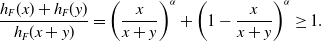 \begin{align*}\frac{h_F(x)+h_F(y)}{h_F(x+y)}=\left(\frac{x}{x+y}\right)^\alpha+\left(1-\frac{x}{x+y}\right)^\alpha\ge 1.\end{align*}
As $h_F$
is additive when
$h_F$
is additive when $\alpha=1$
, Fréchet(1) distribution can be thought as a “boundary” of class
$\alpha=1$
, Fréchet(1) distribution can be thought as a “boundary” of class $\mathcal{H}$
.
$\mathcal{H}$
.
Example 2 (Pareto(1) distribution). For $\alpha\gt 0$
, the Pareto distribution, denoted by Pareto
$\alpha\gt 0$
, the Pareto distribution, denoted by Pareto $(\alpha)$
, is defined as
$(\alpha)$
, is defined as
 \begin{align*}F(x)=1-\frac{1}{(x+1)^\alpha}, x\gt 0.\end{align*}
Pareto $(\alpha)$
distributions have infinite mean if
$(\alpha)$
distributions have infinite mean if $\alpha\le 1$
. Taking second derivative of
$\alpha\le 1$
. Taking second derivative of $h_F$
when
$h_F$
when $\alpha=1$
, we have
$\alpha=1$
, we have $h''_F(x)=-1/(x+1)^2.$
Hence,
$h''_F(x)=-1/(x+1)^2.$
Hence, $h_F$
is concave and
$h_F$
is concave and $\textrm{Pareto}(1)\in\mathcal{H}_s$
.
$\textrm{Pareto}(1)\in\mathcal{H}_s$
.
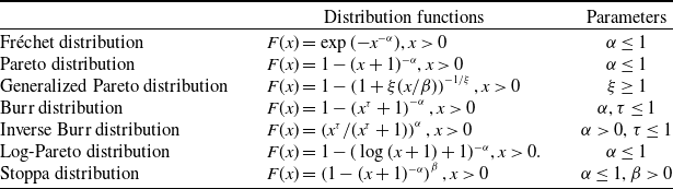
We can show that Pareto $(\alpha)$
with
$(\alpha)$
with $\alpha\le 1$
, as well as many other infinite-mean distributions in Table 1 also belong to
$\alpha\le 1$
, as well as many other infinite-mean distributions in Table 1 also belong to $\mathcal{H}$
either directly using the definition or using some closure properties of
$\mathcal{H}$
either directly using the definition or using some closure properties of $\mathcal{H}$
in Propositions 2 and 3 provided below; see Appendix for detailed derivations of examples in Table 1 and the proofs of Propositions 2 and 3.
$\mathcal{H}$
in Propositions 2 and 3 provided below; see Appendix for detailed derivations of examples in Table 1 and the proofs of Propositions 2 and 3.
Table 1. Examples of distributions in $\mathcal{H}$
.
$\mathcal{H}$
.
Proposition 2. Let $X\sim F$
where
$X\sim F$
where $F\in \mathcal{H}$
. The following statements hold.
$F\in \mathcal{H}$
. The following statements hold.
-
(i) If F is strictly increasing on
$[0,\infty)$
and
$\mathbb{P}(X\lt \infty)=1$
, then F is continuous on
$[0,\infty)$
. -
(ii) For
$\beta\gt 0$
,
$F^\beta\in \mathcal{H}$
. -
(iii) If, in addition, a random variable
$Y\sim G$
, where
$G\in\mathcal{H}$
, is independent of X, then
$\max\{X,Y\}\in \mathcal{H}$
. In terms of distribution functions, if
$F,G\in\mathcal{H}$
, then
$FG\in\mathcal{H}$
. -
(iv) For a nondecreasing, convex, and nonconstant function
$f\,:\,\mathbb{R}_+\rightarrow \mathbb{R}_+$
with
$f(0)=0$
,
$f(X)\in\mathcal{H}$
.


Proposition 3. Let $\bar{\theta} \in \Delta_n^+$
. If distribution functions
$\bar{\theta} \in \Delta_n^+$
. If distribution functions $F_1,\dots,F_n\in\mathcal{H}$
and
$F_1,\dots,F_n\in\mathcal{H}$
and $F_1\le_\textrm{st }\dots\le_\textrm{st }F_n$
, then
$F_1\le_\textrm{st }\dots\le_\textrm{st }F_n$
, then $\sum_{i=1}^n\theta_iF_i\in\mathcal{H}$
.
$\sum_{i=1}^n\theta_iF_i\in\mathcal{H}$
.
It is clear that the various transforms of distributions in Proposition 2 from our class generate many different distributions, showing that the class $\mathcal H$
is indeed rather large. Suppose that
$\mathcal H$
is indeed rather large. Suppose that $F_1,\dots,F_n$
are Pareto distributions with possibly different tail parameters
$F_1,\dots,F_n$
are Pareto distributions with possibly different tail parameters $0\lt \alpha_1,\dots,\alpha_n\le 1$
. As
$0\lt \alpha_1,\dots,\alpha_n\le 1$
. As $F_1,\dots,F_n$
are comparable in stochastic order, by Proposition 3, mixtures of
$F_1,\dots,F_n$
are comparable in stochastic order, by Proposition 3, mixtures of $F_1,\dots,F_n$
are in
$F_1,\dots,F_n$
are in $\mathcal{H}$
.
$\mathcal{H}$
.
3.2 Negative lower orthant dependence
The notion of negative dependence below will be used to establish the main result of this section.
Definition 3 (Block et al., Reference Block, Savits and Shaked1982). Random variables $X_1,\dots,X_n$
are negatively lower orthant dependent (NLOD) if for all
$X_1,\dots,X_n$
are negatively lower orthant dependent (NLOD) if for all $x_1,\dots,x_n \in\mathbb{R}$
,
$x_1,\dots,x_n \in\mathbb{R}$
, $\mathbb{P}(X_1\le x_1,\dots,X_n\le x_n)\le \prod_{i=1}^n\mathbb{P}(X_i\le x_i)$
.
$\mathbb{P}(X_1\le x_1,\dots,X_n\le x_n)\le \prod_{i=1}^n\mathbb{P}(X_i\le x_i)$
.
Negative lower orthant dependence includes independence as a special case. It is commonly used in various research areas, and it is implied by other popular notions of negative dependence in the literature, such as negative association (Alam and Saxena, Reference Alam and Saxena1981 and Joag-Dev and Proschan, Reference Joag-Dev and Proschan1983), negative orthant dependence (Block et al., Reference Block, Savits and Shaked1982), and negative regression dependence (Lehmann, Reference Lehmann1966 and Block et al., Reference Block, Savits and Shaked1985) see, for example, Chi et al. (Reference Chi, Ramdas and Wang2024) for the implications of these notions.
3.3 Main result
Theorem 1. If a random variable $X\in \mathcal{H}$
and random variables
$X\in \mathcal{H}$
and random variables $X_1,\dots,X_n$
are NLOD with marginal laws equal to X, then for
$X_1,\dots,X_n$
are NLOD with marginal laws equal to X, then for $\bar{\theta} \in\Delta_n^+$
,
$\bar{\theta} \in\Delta_n^+$
,
 \begin{equation} X \le_\textrm{st} \theta_1 X_1 + \dots + \theta_n X_n.\end{equation}
If $X\in\mathcal{H}_s$
, then
$X\in\mathcal{H}_s$
, then $X \lt _\textrm{st}\sum_{i=1}^n\theta_{i}X_{i}$
.
$X \lt _\textrm{st}\sum_{i=1}^n\theta_{i}X_{i}$
.
Proof. Let $X\sim F$
and
$X\sim F$
and $\bar \theta\in\Delta_n^+$
. We have, for all
$\bar \theta\in\Delta_n^+$
. We have, for all $x\gt 0$
,
$x\gt 0$
,
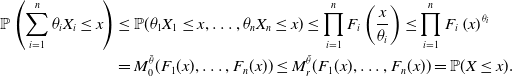
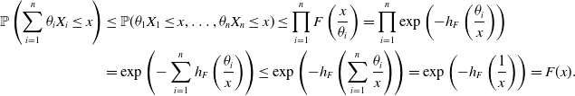 \begin{align*}\mathbb{P}\left(\sum_{i=1}^n\theta_{i}X_{i}\le x\right)&\le \mathbb{P}(\theta_1X_1\le x,\dots,\theta_nX_n\le x) \le \prod_{i=1}^n F\left(\frac{x}{\theta_i}\right)= \prod_{i=1}^n \exp\left(-h_F\left(\frac{\theta_i}{x}\right)\right)\\&= \exp\left(- \sum_{i=1}^nh_F\left(\frac{\theta_i}{x}\right)\right)\le \exp\left(- h_F\left(\sum_{i=1}^n\frac{\theta_i}{x}\right)\right)=\exp\left(- h_F\left(\frac{1}{x}\right)\right)=F(x).\end{align*}
The strictness statement is straightforward. The proof is complete.
An immediate consequence of Theorem 1 and Proposition 1 (i) is that all distributions in $\mathcal{H}$
have infinite mean.
$\mathcal{H}$
have infinite mean.
Remark 2 (Value-at-Risk). One regulatory risk measure in insurance and finance is Value-at-Risk (VaR). For a random variable $X\sim F$
and
$X\sim F$
and $p\in (0,1)$
, VaR is defined as
$p\in (0,1)$
, VaR is defined as $\mathrm{VaR}_{p}(X)=F^{-1}(p)$
. For two random variables X and Y, it is well known that
$\mathrm{VaR}_{p}(X)=F^{-1}(p)$
. For two random variables X and Y, it is well known that $X\le_\textrm{st} Y$
if and only if
$X\le_\textrm{st} Y$
if and only if $\mathrm{VaR}_p(X)\le \mathrm{VaR}_p(Y)$
for all
$\mathrm{VaR}_p(X)\le \mathrm{VaR}_p(Y)$
for all $p\in(0,1)$
. Note that VaR is comonotonic-additive; a risk measure
$p\in(0,1)$
. Note that VaR is comonotonic-additive; a risk measure $\rho$
is comonotonic-additive if
$\rho$
is comonotonic-additive if $\rho(Y+Z)=\rho(Y)+\rho(Z)$
for comonotonic random variables Y and Z.Footnote 1 Then we have
$\rho(Y+Z)=\rho(Y)+\rho(Z)$
for comonotonic random variables Y and Z.Footnote 1 Then we have $\mathrm{VaR}_p(X)=\sum_{i=1}^n\mathrm{VaR}_p(\theta_iX_i)$
for identically distributed random variables
$\mathrm{VaR}_p(X)=\sum_{i=1}^n\mathrm{VaR}_p(\theta_iX_i)$
for identically distributed random variables $X_1,\dots,X_n$
. By Theorem 1, superadditivity of VaR holds for
$X_1,\dots,X_n$
. By Theorem 1, superadditivity of VaR holds for $\bar{\theta}\in\Delta_n^+$
and identically distributed risks
$\bar{\theta}\in\Delta_n^+$
and identically distributed risks $X_1,\dots,X_n\in \mathcal{H}$
that are NLOD: For all
$X_1,\dots,X_n\in \mathcal{H}$
that are NLOD: For all $p\in(0,1)$
,
$p\in(0,1)$
, $ \mathrm{VaR}_p(\theta_1 X_{1})+\dots+\mathrm{VaR}_p(\theta_n X_{n})\le \mathrm{VaR}_p(\theta_{1}X_{1}+\dots+\theta_{n}X_{n}).$
More generally, the superadditivity property holds for any comonotonic-additive risk measure that is consistent with stochastic order.
$ \mathrm{VaR}_p(\theta_1 X_{1})+\dots+\mathrm{VaR}_p(\theta_n X_{n})\le \mathrm{VaR}_p(\theta_{1}X_{1}+\dots+\theta_{n}X_{n}).$
More generally, the superadditivity property holds for any comonotonic-additive risk measure that is consistent with stochastic order.
Remark 3 (Heavy-tailed distributions). A distribution F is said to be heavy-tailed in the sense of Falk et al. (Reference Falk, Hüsler and Reiss2011) with tail parameter $\alpha\gt 0$
, if
$\alpha\gt 0$
, if $\overline F(x)= L(x)x^{-\alpha}$
where L is a slowly varying function, that is,
$\overline F(x)= L(x)x^{-\alpha}$
where L is a slowly varying function, that is, $L(tx)/L(x)\rightarrow 1$
as
$L(tx)/L(x)\rightarrow 1$
as $x\rightarrow \infty$
for all
$x\rightarrow \infty$
for all $t\gt 0$
. For iid heavy-tailed random variables
$t\gt 0$
. For iid heavy-tailed random variables $X_1,X_2,\dots\sim F$
, if there exist sequences of constants
$X_1,X_2,\dots\sim F$
, if there exist sequences of constants $\{a_n\}$
and
$\{a_n\}$
and $\{b_n\}$
where
$\{b_n\}$
where $b_n\gt 0$
such that
$b_n\gt 0$
such that $(\max\{X_1,\dots,X_n\}-a_n)/b_n$
converges to the Fréchet distribution, F is said to be in the maximum domain attraction of the Fréchet distribution. It is known in the Extreme Value Theory (Embrechts et al., Reference Embrechts, Klüppelberg and Mikosch1997) that a distribution is in the maximum domain of attraction of the Fréchet distribution if and only if the distribution is heavy-tailed. Note that for a heavy-tailed random variable X with
$(\max\{X_1,\dots,X_n\}-a_n)/b_n$
converges to the Fréchet distribution, F is said to be in the maximum domain attraction of the Fréchet distribution. It is known in the Extreme Value Theory (Embrechts et al., Reference Embrechts, Klüppelberg and Mikosch1997) that a distribution is in the maximum domain of attraction of the Fréchet distribution if and only if the distribution is heavy-tailed. Note that for a heavy-tailed random variable X with $\alpha\le 1$
,
$\alpha\le 1$
, $\mathbb{E}(|X|)=\infty$
. An interesting property of heavy-tailed risks with infinite mean is the asymptotic superadditivity of VaR: If
$\mathbb{E}(|X|)=\infty$
. An interesting property of heavy-tailed risks with infinite mean is the asymptotic superadditivity of VaR: If $X_1,\dots,X_n$
are iid and heavy-tailed with tail parameter
$X_1,\dots,X_n$
are iid and heavy-tailed with tail parameter $\alpha\lt 1$
,
$\alpha\lt 1$
,
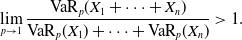 \begin{align*}\lim_{p\rightarrow 1}\frac{\mathrm{VaR}_p(X_1+\dots+X_n)}{\mathrm{VaR}_p(X_1)+\dots+\mathrm{VaR}_p(X_n)}\gt 1.\end{align*}
See, for example, Example 3.1 of Embrechts et al. (Reference Embrechts, Lambrigger and Wüthrich2009) for the claim above. Heavy-tailed risks with infinite mean are not necessarily in $\mathcal{H}$
as the condition of
$\mathcal{H}$
as the condition of $\mathcal{H}$
applies over the whole range of distributions, whereas heavy-tailed distributions have power-law shapes only in their tail parts. On the other hand, risks in
$\mathcal{H}$
applies over the whole range of distributions, whereas heavy-tailed distributions have power-law shapes only in their tail parts. On the other hand, risks in $\mathcal{H}$
are not necessarily heavy-tailed in the sense of Falk et al. (Reference Falk, Hüsler and Reiss2011). For instance, the survival distributions of log-Pareto risks are slowly varying functions. Distributions with slowly varying tails are called super heavy-tailed.
$\mathcal{H}$
are not necessarily heavy-tailed in the sense of Falk et al. (Reference Falk, Hüsler and Reiss2011). For instance, the survival distributions of log-Pareto risks are slowly varying functions. Distributions with slowly varying tails are called super heavy-tailed.
Remark 4 (Convex order). Besides stochastic order, another popular notion of stochastic dominance to compare risks is convex order. For two random variables X and Y, X is said to be smaller than Y in convex order, denoted by $X\le_\textrm{cx}Y$
, if
$X\le_\textrm{cx}Y$
, if $\mathbb{E}(u(X))\le \mathbb{E}(u(Y))$
for all convex functions u provided that the expectations exist. The interpretation of
$\mathbb{E}(u(X))\le \mathbb{E}(u(Y))$
for all convex functions u provided that the expectations exist. The interpretation of $X\le_\textrm{cx}Y$
is that Y is more “spread-out” than X. If
$X\le_\textrm{cx}Y$
is that Y is more “spread-out” than X. If $X_1,\dots,X_n$
are iid and have a finite mean, by Theorem 3.A.35 of Shaked and Shanthikumar (Reference Shaked and Shanthikumar2007), for
$X_1,\dots,X_n$
are iid and have a finite mean, by Theorem 3.A.35 of Shaked and Shanthikumar (Reference Shaked and Shanthikumar2007), for $\bar{\theta}\in\Delta_n^+$
,
$\bar{\theta}\in\Delta_n^+$
, $\sum_{i=1}^n\theta_iX_i\le_\textrm{cx}X_1$
. Unlike Theorem 1, this leads to a diversification benefit. Note that
$\sum_{i=1}^n\theta_iX_i\le_\textrm{cx}X_1$
. Unlike Theorem 1, this leads to a diversification benefit. Note that $\le_\textrm{cx}$
is not suitable for the analysis of risks with infinite mean as the expectation of any increasing convex transform of these risks is infinity.
$\le_\textrm{cx}$
is not suitable for the analysis of risks with infinite mean as the expectation of any increasing convex transform of these risks is infinity.
Remark 5 (Positive dependence). One may expect positive dependence to make larger values of the sum in (3.1) more likely and thus the sum more likely to stochastically dominate a single random variable. We believe that this intuition does not hold due to the very heavy tails of the random variables under consideration. It is known, for instance, that very large values of the sum of iid random variables with heavy tails are likely caused by a single random variable taking a large value, while other random variables are moderate. If random variables are positively dependent and some of them do not take large values, it makes others more likely to take moderate values too, hence positive dependence may hinder large values; see Alink et al. (Reference Alink, Löwe and Wüthrich2004) and Mainik and Rüschendorf (Reference Mainik and Rüschendorf2010) for such observations in some asymptotic senses. These phenomena can also be seen from the deadly risks considered by Müller (2024): For all $i\in[n]$
,
$i\in[n]$
, $\mathbb{P}(X_i=0)=1-p$
and
$\mathbb{P}(X_i=0)=1-p$
and $\mathbb{P}(X_i=\infty)=p$
where
$\mathbb{P}(X_i=\infty)=p$
where $p\gt 0$
. For
$p\gt 0$
. For $\overline \theta\in\Delta_n^+$
, it is clear that
$\overline \theta\in\Delta_n^+$
, it is clear that $\sum_{i=1}^n\theta_iX_i=\infty$
as long as one of
$\sum_{i=1}^n\theta_iX_i=\infty$
as long as one of $X_1,\dots,X_n$
is
$X_1,\dots,X_n$
is $\infty$
. If
$\infty$
. If $X_1,\dots,X_n$
are positively lower orthant dependent (PLOD), that is
$X_1,\dots,X_n$
are positively lower orthant dependent (PLOD), that is $\mathbb{P}(X_1\le x_1,\dots,X_n\le x_n)\ge \prod_{i=1}^n\mathbb{P}(X_i\le x_i)$
for all
$\mathbb{P}(X_1\le x_1,\dots,X_n\le x_n)\ge \prod_{i=1}^n\mathbb{P}(X_i\le x_i)$
for all $x_1,\dots,x_n \in\mathbb{R}$
, then
$x_1,\dots,x_n \in\mathbb{R}$
, then
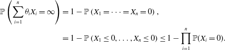 \begin{align*}\mathbb{P}\left(\sum_{i=1}^n\theta_iX_i=\infty\right)&=1-\mathbb{P}\left(X_1=\dots=X_n=0\right),\\&=1-\mathbb{P}\left(X_1\le 0,\dots,X_n\le0\right)\le 1-\prod_{i=1}^n\mathbb{P}(X_i= 0).\end{align*}
Hence, $\sum_{i=1}^n\theta_iX_i$
is stochastically smaller when
$\sum_{i=1}^n\theta_iX_i$
is stochastically smaller when $X_1,\dots,X_n$
are PLOD compared to the case when
$X_1,\dots,X_n$
are PLOD compared to the case when $X_1,\dots,X_n$
are independent. The situation is reversed for NLOD random variables. However, (SD) still holds for PLOD risks
$X_1,\dots,X_n$
are independent. The situation is reversed for NLOD random variables. However, (SD) still holds for PLOD risks $X_1,\dots,X_n$
as
$X_1,\dots,X_n$
as
 \begin{align*}\mathbb{P}\left(\sum_{i=1}^n\theta_iX_i=\infty\right)=1-\mathbb{P}\left(X_1=\dots=X_n=0\right)\ge 1-\mathbb{P}(X_1=0)=\mathbb{P}(X_1=\infty).\end{align*}
In Chen et al. (Reference Chen, Hu, Wang and Zou2025b), (SD) is shown to hold for infinite-mean Pareto random variables that are positively dependent via some specific Clayton copula.
4. Weighted sums of non-identically distributed risks
In the previous section, property (SD) is studied for risks with the same marginal distribution. We now look at the case when risks are not necessarily identically distributed. Given non-identically distributed random variables $X_1, \dots, X_n$
and any
$X_1, \dots, X_n$
and any $\bar{\theta}\in\Delta_n$
, the question is to study for which random variable X the following property holds
$\bar{\theta}\in\Delta_n$
, the question is to study for which random variable X the following property holds
 \begin{equation} X \le_\textrm{st} \theta_1 X_1 + \dots + \theta_n X_n.\end{equation}
To study this problem, we introduce the class of super-Fréchet distributions defined below.
Definition 4. A random variable X is said to be super-Fréchet (or has a super-Fréchet distribution) if X and f(Y) have the same distribution, where $Y\sim$
Fréchet(1) and f is a strictly increasing and convex function with
$Y\sim$
Fréchet(1) and f is a strictly increasing and convex function with $f(0)=0$
.
$f(0)=0$
.
As convex transforms make the tail of random variables heavier, super-Fréchet distributions are more heavy-tailed than Fréchet(1) distribution, and thus the name. It is easy to check that a random variable X with $\textrm{ess-inf}\ X=0$
is super-Fréchet if and only if the function
$\textrm{ess-inf}\ X=0$
is super-Fréchet if and only if the function $g\,:\,x\mapsto 1/({-}\log \mathbb{P}(X\le x)) $
is strictly increasing and concave on
$g\,:\,x\mapsto 1/({-}\log \mathbb{P}(X\le x)) $
is strictly increasing and concave on $(0,\infty)$
with
$(0,\infty)$
with $\lim_{x\downarrow 0}g(x)=0$
.
$\lim_{x\downarrow 0}g(x)=0$
.
As Fréchet(1) distribution is in $\mathcal{H}$
, by Proposition 1 (iv), Super-Fréchet distributions are in
$\mathcal{H}$
, by Proposition 1 (iv), Super-Fréchet distributions are in $\mathcal{H}$
. On the other hand, not all distributions in
$\mathcal{H}$
. On the other hand, not all distributions in $\mathcal{H}$
are Super-Fréchet, which can be seen from the following example.
$\mathcal{H}$
are Super-Fréchet, which can be seen from the following example.
Example 3. For $c\gt 0$
, define a distribution function on
$c\gt 0$
, define a distribution function on $(0,\infty]$
:
$(0,\infty]$
:
 \begin{align*}F(x)=\exp({-}c\lceil1/x\rceil),\mbox{for}\ x\in(0,\infty),\end{align*}
and $F(\infty)=1$
. Then
$F(\infty)=1$
. Then $h_F(x)=c \lceil x\rceil $
,
$h_F(x)=c \lceil x\rceil $
, $x\in(0,\infty)$
, is subadditive, and thus
$x\in(0,\infty)$
, is subadditive, and thus $F\in \mathcal{H}$
. However, since F is not a continuous distribution, it is not super-Fréchet. The distributions in this example are the so-called inverse-geometric distributions, also considered in Example 2.7 of Arab et al. (Reference Arab, Lando and Oliveira2024).
$F\in \mathcal{H}$
. However, since F is not a continuous distribution, it is not super-Fréchet. The distributions in this example are the so-called inverse-geometric distributions, also considered in Example 2.7 of Arab et al. (Reference Arab, Lando and Oliveira2024).
Fréchet distributions with infinite mean, as well as many other distributions in the following example, are super-Fréchet.
Example 4. Pareto, Burr, paralogistic, and log-logistic random variables, all with infinite mean, are super-Fréchet distributions. Since all these random variables can be obtained by applying strictly increasing and convex transforms to Pareto(1) random variables (see Appendix C), it suffices to show that a Pareto(1) random variable is super-Fréchet. Write the Pareto(1) distribution as $F(x)=1-1/(x+1)=\exp({-}1/g(x))$
,
$F(x)=1-1/(x+1)=\exp({-}1/g(x))$
, $x\gt 0$
, where
$x\gt 0$
, where $g(x)=1/\log(1+1/x)$
. It is clear that g is strictly increasing and
$g(x)=1/\log(1+1/x)$
. It is clear that g is strictly increasing and $\lim_{x\downarrow 0}g(x)=0$
. We show g is concave on
$\lim_{x\downarrow 0}g(x)=0$
. We show g is concave on $(0,\infty)$
. We have
$(0,\infty)$
. We have
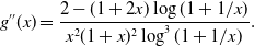 \begin{align*}g''(x)=\frac{2 - (1 + 2 x) \log(1 + 1/x)}{x^2 (1 + x)^2 \log^3(1 + 1/x)}.\end{align*}
Let $r(x)=\log\left(1/x+1\right)-2/(1+2x)$
,
$r(x)=\log\left(1/x+1\right)-2/(1+2x)$
, $x\gt 0$
. It is easy to verify that r is strictly decreasing on
$x\gt 0$
. It is easy to verify that r is strictly decreasing on $(0,\infty)$
and r(x) goes to 0 as x goes to infinity. Thus,
$(0,\infty)$
and r(x) goes to 0 as x goes to infinity. Thus, $r(x)\gt 0$
and
$r(x)\gt 0$
and $g''(x)\lt 0$
for
$g''(x)\lt 0$
for $x\in(0,\infty)$
.
$x\in(0,\infty)$
.
We will assume $X_1,\dots,X_n$
in (4.1) are super-Fréchet. Since
$X_1,\dots,X_n$
in (4.1) are super-Fréchet. Since $X_1,\dots,X_n$
may not have the same distribution, how to choose the distribution of X is not clear. A perhaps natural candidate is the generalized mean of the distributions of
$X_1,\dots,X_n$
may not have the same distribution, how to choose the distribution of X is not clear. A perhaps natural candidate is the generalized mean of the distributions of $X_1,\dots,X_n$
. For
$X_1,\dots,X_n$
. For $r\in \mathbb{R}\setminus \{0\}$
,
$r\in \mathbb{R}\setminus \{0\}$
, $n\in \mathbb{N}$
, and
$n\in \mathbb{N}$
, and $\textbf w=(w_1,\dots,w_n)\in \Delta_n$
, the generalized r-mean function is defined as
$\textbf w=(w_1,\dots,w_n)\in \Delta_n$
, the generalized r-mean function is defined as
 \begin{align*}M^{\textbf w}_r(u_1,\dots,u_n) = \left(w_1 u_1^r+\dots+w_n u_n^r \right)^{1/r}, (u_1,\dots,u_n) \in (0,\infty)^{n}.\end{align*}
The generalized 0-mean function is the weighted geometric mean, that is, $M^{\textbf w}_0(u_1,\dots,u_n) =\prod_{i=1}^n u_i^{w_i},$
which is also the limit of
$M^{\textbf w}_0(u_1,\dots,u_n) =\prod_{i=1}^n u_i^{w_i},$
which is also the limit of $M^{\textbf w}_r$
as
$M^{\textbf w}_r$
as $r\to 0$
. A generalized mean of distribution functions is a distribution function. In particular, if
$r\to 0$
. A generalized mean of distribution functions is a distribution function. In particular, if $r=1$
, it leads to a distribution mixture model, that is, if
$r=1$
, it leads to a distribution mixture model, that is, if $X\sim M^{ \textbf w}_1(F_1,\dots,F_n)$
, X has the same distribution as
$X\sim M^{ \textbf w}_1(F_1,\dots,F_n)$
, X has the same distribution as $\sum_{i=1}^nX_i{\unicode{x1D7D9}}_{A_i}$
where
$\sum_{i=1}^nX_i{\unicode{x1D7D9}}_{A_i}$
where $A_1,\dots,A_n$
are mutually exclusive, independent of
$A_1,\dots,A_n$
are mutually exclusive, independent of $X_1,\dots,X_n$
, and
$X_1,\dots,X_n$
, and $\mathbb{P}(A_i)=w_i$
for all
$\mathbb{P}(A_i)=w_i$
for all $i\in[n]$
.
$i\in[n]$
.
Theorem 2. If $X_1,\dots,X_n$
are super-Fréchet and NLOD with
$X_1,\dots,X_n$
are super-Fréchet and NLOD with $X_i\sim F_i$
,
$X_i\sim F_i$
, $i\in[n]$
, and
$i\in[n]$
, and $X\sim M^{\bar \theta}_r(F_1,\dots,F_n)$
for some
$X\sim M^{\bar \theta}_r(F_1,\dots,F_n)$
for some $r\ge 0$
, then for
$r\ge 0$
, then for $\bar{\theta}\in\Delta_n^+$
,
$\bar{\theta}\in\Delta_n^+$
,
 \begin{equation*}X \le_\textrm{st} \theta_1 X_1 + \dots + \theta_n X_n.\end{equation*}
Proof. Let $g_i(x)=1/({-}\log F_i(x))$
,
$g_i(x)=1/({-}\log F_i(x))$
, $x\gt 0$
, for all
$x\gt 0$
, for all $i\in[n]$
. As
$i\in[n]$
. As $g_i$
,
$g_i$
, $i\in[n]$
, is strictly increasing and concave on
$i\in[n]$
, is strictly increasing and concave on $(0,\infty)$
with
$(0,\infty)$
with $\lim_{x\downarrow 0}g_i(x)=0$
,
$\lim_{x\downarrow 0}g_i(x)=0$
, $ g_i(x)\ge \theta g_i(x/\theta)$
for all
$ g_i(x)\ge \theta g_i(x/\theta)$
for all $x\gt 0$
and
$x\gt 0$
and $\theta\in(0,1)$
. Then, for
$\theta\in(0,1)$
. Then, for $\theta\in(0,1)$
,
$\theta\in(0,1)$
,
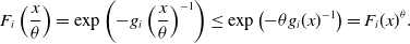 \begin{align} F_i\left(\frac{x}{\theta}\right)=\exp\left(-g_i\left(\frac{x}{\theta}\right)^{-1}\right)\le \exp\left(-\theta g_i(x)^{-1}\right)=F_i(x)^\theta. \end{align}
As $X_1,\dots,X_n$
are NLOD, by 4.2, for any
$X_1,\dots,X_n$
are NLOD, by 4.2, for any $x\gt 0$
,
$x\gt 0$
, $(\theta_1,\dots,\theta_n)\in\Delta_n$
, and
$(\theta_1,\dots,\theta_n)\in\Delta_n$
, and $r\ge 0$
,
$r\ge 0$
,
 \begin{align*}\mathbb{P}\left(\sum_{i=1}^n\theta_{i}X_{i}\le x\right)&\le \mathbb{P}(\theta_1X_1\le x,\dots,\theta_nX_n\le x)\le \prod_{i=1}^n F_i\left(\frac{x}{\theta_i}\right) \le\prod_{i=1}^n F_i\left(x\right)^{\theta_i}\\&=M^{\bar \theta}_0(F_1(x),\dots,F_n(x))\le M^{\bar \theta}_r(F_1(x),\dots,F_n(x))=\mathbb{P}(X\le x).\end{align*}
The last inequality is because the generalized mean function is monotone in r; that is, given any $\textbf w\in \Delta_n$
,
$\textbf w\in \Delta_n$
, $M^{\textbf w}_r\le M^{\textbf w}_s$
for
$M^{\textbf w}_r\le M^{\textbf w}_s$
for $r\le s $
(Theorem 16 of Hardy et al., Reference Hardy, Littlewood and Pólya1934).
$r\le s $
(Theorem 16 of Hardy et al., Reference Hardy, Littlewood and Pólya1934).
5. Comparison with existing results
In this section, we compare our results with the literature. We first consider the case when $X_1,\dots,X_n$
in (SD) are iid. In Arab et al. (Reference Arab, Lando and Oliveira2024), it is shown that (SD) holds for nonnegative random variables that are InvSub; a random variable
$X_1,\dots,X_n$
in (SD) are iid. In Arab et al. (Reference Arab, Lando and Oliveira2024), it is shown that (SD) holds for nonnegative random variables that are InvSub; a random variable $X\sim F$
and its distribution is called InvSub if
$X\sim F$
and its distribution is called InvSub if $1-F(1/x)$
is subadditive. The class of InvSub distributions is larger than
$1-F(1/x)$
is subadditive. The class of InvSub distributions is larger than $\mathcal{H}$
as
$\mathcal{H}$
as $h_F=-\log F(1/x)$
is subadditive implies that
$h_F=-\log F(1/x)$
is subadditive implies that $1-F(1/x)$
is subadditive. Müller (2024) showed that (SD) holds for super-Cauchy random variables; a random variable
$1-F(1/x)$
is subadditive. Müller (2024) showed that (SD) holds for super-Cauchy random variables; a random variable $X\sim F$
and its distribution is called super-Cauchy if
$X\sim F$
and its distribution is called super-Cauchy if $F^{-1}(G(x))$
is convex where G is the standard Cauchy distribution function. Super-Cauchy distributions are continuous and can take positive values on the entire real line but they do not contain
$F^{-1}(G(x))$
is convex where G is the standard Cauchy distribution function. Super-Cauchy distributions are continuous and can take positive values on the entire real line but they do not contain $\mathcal{H}$
as
$\mathcal{H}$
as $\mathcal{H}$
includes non-continuous distributions (see Example 3). The proofs in both Arab et al. (Reference Arab, Lando and Oliveira2024) and Müller (2024) are short and elegant.
$\mathcal{H}$
includes non-continuous distributions (see Example 3). The proofs in both Arab et al. (Reference Arab, Lando and Oliveira2024) and Müller (2024) are short and elegant.
As our results cover the case of negatively dependent risks, for the rest of this section, we will focus on the comparison of our results with Chen et al. (Reference Chen, Embrechts and Wang2025a); to our best knowledge, Chen et al. (Reference Chen, Embrechts and Wang2025a) is the only other paper that deals with negatively dependent risks. Chen et al. (Reference Chen, Embrechts and Wang2025a) showed that
 \begin{equation} \textrm{(SD)}\ \mbox{holds for super-Pareto risks $X_1,\dots,X_n$ that are weakly negatively associated.} \end{equation}
For ease of comparison, definitions of super-Pareto distributions and weak negative association are given in a slightly different form from Chen et al. (Reference Chen, Embrechts and Wang2025a) below.
Definition 5. A random variable X and its distribution is super-Pareto if X and f(Y) have the same distribution for some non-decreasing, convex, and non-constant function f with $f(0)=0$
and
$f(0)=0$
and $Y\sim \mathrm{Pareto}(1)$
.
$Y\sim \mathrm{Pareto}(1)$
.
Definition 6. A set $S\subseteq \mathbb{R}^{k}$
,
$S\subseteq \mathbb{R}^{k}$
, $k\in \mathbb{N}$
is decreasing if
$k\in \mathbb{N}$
is decreasing if $\textbf x\in S$
implies
$\textbf x\in S$
implies $\textbf y\in S$
for all
$\textbf y\in S$
for all $\textbf y\le \textbf x$
. Random variables
$\textbf y\le \textbf x$
. Random variables $X_1,\dots,X_n$
are weakly negatively associated if for any
$X_1,\dots,X_n$
are weakly negatively associated if for any $i\in[n]$
, decreasing set
$i\in[n]$
, decreasing set $S \subseteq \mathbb{R}^{n-1}$
, and
$S \subseteq \mathbb{R}^{n-1}$
, and $x\in \mathbb{R}$
with
$x\in \mathbb{R}$
with $\mathbb{P}(X_i\le x)\gt 0$
,
$\mathbb{P}(X_i\le x)\gt 0$
,
 \begin{align*}\mathbb{P}(\textbf X_{-i} \in S, X_i\le x) \le \mathbb{P}(\textbf X_{-i}\in S)\mathbb{P}( X_i\le x).\end{align*}
where $\textbf X_{-i}=(X_1,\dots,X_{i-1}, X_{i+1},\dots,X_n)$
.
$\textbf X_{-i}=(X_1,\dots,X_{i-1}, X_{i+1},\dots,X_n)$
.
Lemma 1. If random variables $X_1,\dots,X_n$
are super-Pareto and weakly negatively associated, then
$X_1,\dots,X_n$
are super-Pareto and weakly negatively associated, then $X_1,\dots,X_n\in\mathcal{H}$
and they are NLOD.
$X_1,\dots,X_n\in\mathcal{H}$
and they are NLOD.
Proof. As Pareto(1) risks are in $\mathcal{H}$
(see Example 2), by Proposition 2 (iv), super-Pareto risks are in
$\mathcal{H}$
(see Example 2), by Proposition 2 (iv), super-Pareto risks are in $\mathcal{H}$
. Since
$\mathcal{H}$
. Since $X_1,\dots,X_n$
are weakly negatively associated, for any
$X_1,\dots,X_n$
are weakly negatively associated, for any $(x_1,\dots,x_n)\in \mathbb{R}^n$
,
$(x_1,\dots,x_n)\in \mathbb{R}^n$
,
 \begin{align*}\mathbb{P}(X_1\le x_1,\dots,X_n\le x_n)\le \mathbb{P}(X_1\le x_1,\dots,X_{n-1}\le x_{n-1})\mathbb{P}(X_n\le n)\le \prod_{i=1}^n\mathbb{P}(X_i\le x_i).\end{align*}
Thus, $X_1,\dots,X_n$
are NLOD.
$X_1,\dots,X_n$
are NLOD.
The above lemma shows that Theorem 1 implies (5.1), which is in Theorem 1 (i) of Chen et al.(Reference Chen, Embrechts and Wang2025a). We present below a corollary, which leads to a similar result as Theorem 1 (ii) of Chen et al. (Reference Chen, Embrechts and Wang2025a).
Corollary 1. Suppose that a random variable $X\in\mathcal{H}$
, random variables
$X\in\mathcal{H}$
, random variables $X_1,\dots,X_n$
are NLOD with marginal laws equal to X, and
$X_1,\dots,X_n$
are NLOD with marginal laws equal to X, and $\xi_1,\dots,\xi_n$
are any positive random variables independent of
$\xi_1,\dots,\xi_n$
are any positive random variables independent of $X,X_1,\dots,X_n$
with
$X,X_1,\dots,X_n$
with $\sum_{i=1}^n\xi_i\le 1$
. If
$\sum_{i=1}^n\xi_i\le 1$
. If $\mathbb{P}(cX\gt t) \ge c\mathbb{P}(X\gt t) $
for all
$\mathbb{P}(cX\gt t) \ge c\mathbb{P}(X\gt t) $
for all $c \in (0,1]$
and
$c \in (0,1]$
and $t\gt 0$
, then for
$t\gt 0$
, then for $x\ge 0$
,
$x\ge 0$
,
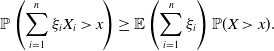 \begin{equation} \mathbb{P}\left(\sum_{i=1}^n\xi_i X_i \gt x\right) \ge \mathbb{E}\left(\sum_{i=1}^n \xi_i\right) \mathbb{P}(X\gt x).\end{equation}
Proof. By Theorem 1 and the independence between $\xi_1,\dots,\xi_n$
and
$\xi_1,\dots,\xi_n$
and $X,X_1,\dots,X_n$
, we have
$X,X_1,\dots,X_n$
, we have
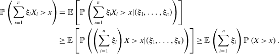 \begin{align*}\mathbb{P}\left(\sum_{i=1}^n\xi_i X_i \gt x\right) &= \mathbb{E}\left[\mathbb{P}\left(\sum_{i=1}^n\xi_i X_i \gt x|(\xi_1,\dots,\xi_n)\right)\right]\\&\ge \mathbb{E}\left[\mathbb{P}\left(\left(\sum_{i=1}^n \xi_i\right) X \gt x|(\xi_1,\dots,\xi_n)\right)\right] \ge \mathbb{E}\left(\sum_{i=1}^n \xi_i\right) \mathbb{P}\left(X \gt x\right). \end{align*}
For $\bar \theta\in\Delta_n$
, let
$\bar \theta\in\Delta_n$
, let $A_1,\dots,A_n$
be any events independent of
$A_1,\dots,A_n$
be any events independent of $(X_1,\dots,X_n)$
and event A be independent of X satisfying
$(X_1,\dots,X_n)$
and event A be independent of X satisfying $\mathbb{P}(A)=\sum_{i=1}^n \theta_i\mathbb{P}(A_i)$
. If
$\mathbb{P}(A)=\sum_{i=1}^n \theta_i\mathbb{P}(A_i)$
. If $X_1,\dots,X_n$
are financial losses,
$X_1,\dots,X_n$
are financial losses, $A_1,\dots,A_n$
can be interpreted as the triggering events for these losses. Let
$A_1,\dots,A_n$
can be interpreted as the triggering events for these losses. Let $\xi_i = \theta_i {\unicode{x1D7D9}}_{A_i}$
. By (5.2), for
$\xi_i = \theta_i {\unicode{x1D7D9}}_{A_i}$
. By (5.2), for $x\ge 0$
,
$x\ge 0$
,
 \begin{align*}\mathbb{P}\left(\sum_{i=1}^n\theta_i X_i{\unicode{x1D7D9}}_{A_i} \gt x\right) \ge \mathbb{E}\left(\sum_{i=1}^n \theta_i {\unicode{x1D7D9}}_{A_i}\right) \mathbb{P}(X\gt x)=\mathbb{P}(A)\mathbb{P}(X\gt x)=\mathbb{P}(X{\unicode{x1D7D9}}_A\gt x),\end{align*}
which is equivalent to
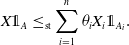 \begin{equation}X{\unicode{x1D7D9}}_A\le_\textrm{st}\sum_{i=1}^n\theta_i X_i{\unicode{x1D7D9}}_{A_i}.\end{equation}
Theorem 1 (ii) of Chen et al. (Reference Chen, Embrechts and Wang2025a) showed (5.3) with different assumptions from Corollary 1; we refer readers to Chen et al. (Reference Chen, Embrechts and Wang2025a) for more details.
6. Conclusion
In this paper, we provide some sufficient conditions for property (SD) to hold. One can see that the property, while very strong, holds for a remarkably large class of distributions. We have also shown that it remains valid for non-identically distributed random variables.
We conclude with some open questions. First, we are interested in understanding how close our sufficient conditions for (SD) are to the optimal ones, that is, we would like to understand what conditions are necessary for (SD).
Second, the definition of our class of heavy-tailed random variables seems to suggest that it is the distribution of $1/X$
that is of importance. We currently lack an intuitive explanation of this.
$1/X$
that is of importance. We currently lack an intuitive explanation of this.
Finally, property (SD) raises the possibility that, for some random variables $X_1,\dots,X_n$
and two vectors
$X_1,\dots,X_n$
and two vectors $\bar{\eta}, \bar{\gamma} \in \mathbb{R}^n_+$
,
$\bar{\eta}, \bar{\gamma} \in \mathbb{R}^n_+$
,
 \begin{equation}\eta_1 X_1 + \dots + \eta_n X_n\le_\textrm{st }\gamma_1 X_1 + \dots + \gamma_n X_n,\end{equation}
where $\bar \gamma$
is smaller than
$\bar \gamma$
is smaller than $\bar \eta$
in majorization order; that is,
$\bar \eta$
in majorization order; that is, $\sum^n_{i=1}\gamma_i =\sum^n_{i=1}\eta_i$
and
$\sum^n_{i=1}\gamma_i =\sum^n_{i=1}\eta_i$
and $\sum^k_{i=1} \gamma_{(i)} \ge \sum^k_{i=1} \eta_{(i)}\,$
for
$\sum^k_{i=1} \gamma_{(i)} \ge \sum^k_{i=1} \eta_{(i)}\,$
for $k\in [n-1]$
where
$k\in [n-1]$
where $\gamma_{(i)}$
and
$\gamma_{(i)}$
and $\eta_{(i)}$
represent the ith smallest order statistics of
$\eta_{(i)}$
represent the ith smallest order statistics of $\bar \gamma$
and
$\bar \gamma$
and $\bar \eta$
. Clearly, (6.1) implies (SD). It is well known that (6.1) holds for iid stable random variables with infinite mean (see Ibragimov, Reference Ibragimov2005), and it was recently shown to hold for iid Pareto random variables with infinite mean by Chen et al.(Reference Chen, Hu, Wang and Zou2025b). It is of question whether (6.1) can hold for a larger class of distributions. Note that the methods used in the current paper do not appear to be useful to address (6.1) as we rely on the comparison of a sum with each of the summands. A more subtle approach to sums is required.
$\bar \eta$
. Clearly, (6.1) implies (SD). It is well known that (6.1) holds for iid stable random variables with infinite mean (see Ibragimov, Reference Ibragimov2005), and it was recently shown to hold for iid Pareto random variables with infinite mean by Chen et al.(Reference Chen, Hu, Wang and Zou2025b). It is of question whether (6.1) can hold for a larger class of distributions. Note that the methods used in the current paper do not appear to be useful to address (6.1) as we rely on the comparison of a sum with each of the summands. A more subtle approach to sums is required.
Acknowledgments
The authors would like to thank two anonymous referees for their helpful comments. The authors also thank Qihe Tang and Ruodu Wang for the valuable discussions and comments on a preliminary version of this paper. Yuyu Chen is supported by the 2025 Early Career Researcher Grant from the University of Melbourne.
Competing interests
The authors declare none.
Appendices
A. Proof of Proposition 2
(i) As $h_F$
is subadditive and increasing, and
$h_F$
is subadditive and increasing, and $\lim_{x\downarrow 0}h_F(x)=0$
,
$\lim_{x\downarrow 0}h_F(x)=0$
, $h_F$
is continuous on
$h_F$
is continuous on $(0,\infty)$
, and so is F (see Remark 1 of Matkowski and Światkowski, Reference Matkowski1993). The desired result is due to the right-continuity of F.
$(0,\infty)$
, and so is F (see Remark 1 of Matkowski and Światkowski, Reference Matkowski1993). The desired result is due to the right-continuity of F.
(ii) Proof of (ii) is straightforward and thus omitted.
(iii) This is also straightforward.
(iv) For $y\ge0$
, let
$y\ge0$
, let $f^{-1+}(y)=\inf\{x\ge 0\,:\,f(x)\gt y\}$
be the right-continuous generalized inverse of f with the convention that
$f^{-1+}(y)=\inf\{x\ge 0\,:\,f(x)\gt y\}$
be the right-continuous generalized inverse of f with the convention that $\inf \emptyset=\infty$
. As f is increasing, convex, and nonconstant with
$\inf \emptyset=\infty$
. As f is increasing, convex, and nonconstant with $f(0)=0$
,
$f(0)=0$
, $f^{-1+}$
is strictly increasing and concave and
$f^{-1+}$
is strictly increasing and concave and $f^{-1+}(0)\ge 0$
. Therefore, by concavity of
$f^{-1+}(0)\ge 0$
. Therefore, by concavity of $f^{-1+}$
and
$f^{-1+}$
and $f^{-1+}(0)\ge 0$
, it is clear that
$f^{-1+}(0)\ge 0$
, it is clear that $f^{-1+}(tx)\ge tf^{-1+}(x)$
for any
$f^{-1+}(tx)\ge tf^{-1+}(x)$
for any $x\gt 0$
and
$x\gt 0$
and $t\in(0,1]$
. For any
$t\in(0,1]$
. For any $a,b\gt 0$
,
$a,b\gt 0$
,
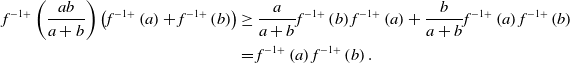 \begin{align*}f^{-1+}\left(\frac{ab}{a+b}\right)\left(f^{-1+}\left(a\right)+f^{-1+}\left(b\right)\right)&\ge \frac{a}{a+b}f^{-1+}\left(b\right)f^{-1+}\left(a\right)+\frac{b}{a+b}f^{-1+}\left(a\right)f^{-1+}\left(b\right)\\&=f^{-1+}\left(a\right)f^{-1+}\left(b\right). \end{align*}
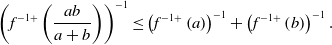
Hence, we have
 \begin{align} \left(f^{-1+}\left(\frac{ab}{a+b}\right)\right)^{-1}\le \left(f^{-1+}\left(a\right)\right)^{-1}+\left(f^{-1+}\left(b\right)\right)^{-1}. \end{align}
Denote by F and G the distribution functions of X and f(X), respectively. Then $G(x)=\mathbb{P}(f(X)\le x)=\mathbb{P}(X\le f^{-1+}(x))=F(f^{-1+}(x))$
for
$G(x)=\mathbb{P}(f(X)\le x)=\mathbb{P}(X\le f^{-1+}(x))=F(f^{-1+}(x))$
for $x\ge0$
. By letting
$x\ge0$
. By letting $g(x)=1/f^{-1+}(1/x)$
for
$g(x)=1/f^{-1+}(1/x)$
for $x\gt 0$
, we write
$x\gt 0$
, we write $h_G=h_F\circ g$
. By inequality (A1), for any
$h_G=h_F\circ g$
. By inequality (A1), for any $x,y\gt 0$
,
$x,y\gt 0$
,
 \begin{align*} g(x+y)=\left(f^{-1+}\left(\frac{1/xy}{1/x+1/y}\right)\right)^{-1}\le \left(f^{-1+}\left(\frac{1}{x}\right)\right)^{-1}+\left(f^{-1+}\left(\frac{1}{y}\right)\right)^{-1}=g(x)+g(y). \end{align*}
Therefore, g is subadditive. As $h_F$
is subadditive and nondecreasing, it is clear that
$h_F$
is subadditive and nondecreasing, it is clear that $h_G=h_F\!\circ\!g$
is subadditive and we have the desired result.
$h_G=h_F\!\circ\!g$
is subadditive and we have the desired result.
B. Proof of Proposition 3
Let $G=\sum_{i=1}^n\theta_iF_i$
. It suffices to show
$G=\sum_{i=1}^n\theta_iF_i$
. It suffices to show
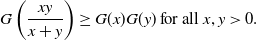 \begin{align}G\left(\frac{xy}{x+y}\right)\ge G(x)G(y)\ \mbox{for all $x,y\gt 0$.} \end{align}
For $n=2$
, as
$n=2$
, as $F_1$
and
$F_1$
and $F_2$
are super heavy-tailed,
$F_2$
are super heavy-tailed,
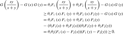 \begin{align*}G\left(\frac{xy}{x+y}\right)-G\left(x\right)G\left(y\right)&=\theta_1F_1\left(\frac{xy}{x+y}\right)+\theta_2F_2\left(\frac{xy}{x+y}\right)-G\left(x\right)G\left(y\right)\\&\ge \theta_1F_1\left(x\right)F_1\left(y\right)+\theta_2F_2\left(x\right)F_2\!\left(y\right)-G\left(x\right)G\left(y\right)\\&=\theta_1F_1\left(x\right)F_1\left(y\right)+\theta_2F_2\left(x\right)F_2\!\left(y\right)\\&-(\theta_1F_1(x)+\theta_2F_2(x))(\theta_1F_1(y)+\theta_2F_2(y))\\&=\theta_1\theta_2(F_1\left(x\right)-F_2(x))(F_1\left(y\right)-F_2(y))\ge 0.\end{align*}
Hence, (B1) holds for $n=2$
. Next, assume that (B1) holds for
$n=2$
. Next, assume that (B1) holds for $n=k-1$
where
$n=k-1$
where $k\gt 3$
is an integer. Let
$k\gt 3$
is an integer. Let $a=\sum_{i=1}^{k-1}\theta_iF_i(x)$
,
$a=\sum_{i=1}^{k-1}\theta_iF_i(x)$
, $b=\sum_{i=1}^{k-1}\theta_iF_i(y)$
,
$b=\sum_{i=1}^{k-1}\theta_iF_i(y)$
, $c=a/(F_n(x)(1-\theta_n))$
, and
$c=a/(F_n(x)(1-\theta_n))$
, and $d=b/(F_n(y)(1-\theta_n))$
. For
$d=b/(F_n(y)(1-\theta_n))$
. For $n=k$
,
$n=k$
,
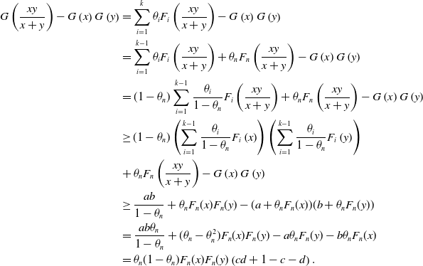 \begin{align*}G\left(\frac{xy}{x+y}\right)-G\left(x\right)G\left(y\right)&=\sum_{i=1}^k\theta_iF_i\left(\frac{xy}{x+y}\right)-G\left(x\right)G\left(y\right)\\&=\sum_{i=1}^{k-1}\theta_iF_i\left(\frac{xy}{x+y}\right)+\theta_nF_n\left(\frac{xy}{x+y}\right)-G\left(x\right)G\left(y\right)\\&=(1-\theta_n)\sum_{i=1}^{k-1}\frac{\theta_i}{1-\theta_n}F_i\left(\frac{xy}{x+y}\right)+\theta_nF_n\left(\frac{xy}{x+y}\right)-G\left(x\right)G\left(y\right)\\&\ge(1-\theta_n)\left(\sum_{i=1}^{k-1}\frac{\theta_i}{1-\theta_n}F_i\left(x\right)\right)\left(\sum_{i=1}^{k-1}\frac{\theta_i}{1-\theta_n}F_i\left(y\right)\right)\\&+\theta_nF_n\left(\frac{xy}{x+y}\right)-G\left(x\right)G\left(y\right)\\&\ge \frac{ab}{1-\theta_n}+\theta_nF_n(x)F_n(y)-(a+\theta_nF_n(x))(b+\theta_nF_n(y))\\&=\frac{ab\theta_n}{1-\theta_n}+(\theta_n-\theta_n^2)F_n(x)F_n(y)-a\theta_nF_n(y)-b\theta_nF_n(x)\\&=\theta_n(1-\theta_n)F_n(x)F_n(y)\left(cd+1-c-d\right).\end{align*}
As $F_1\le_\textrm{st }\dots\le_\textrm{st }F_k$
,
$F_1\le_\textrm{st }\dots\le_\textrm{st }F_k$
, $F_k\le \sum_{i=1}^{k-1}\theta_i/(1-\theta_n)F_i$
. Thus
$F_k\le \sum_{i=1}^{k-1}\theta_i/(1-\theta_n)F_i$
. Thus $c,d\ge 1$
and
$c,d\ge 1$
and $cd+1-c-d\ge 0$
. The proof is complete by induction.
$cd+1-c-d\ge 0$
. The proof is complete by induction.
C. Examples of distributions in the class
$\mathcal{H}$

In this section, we demonstrate that many well-known infinite-mean distributions are in $\mathcal{H}$
.
$\mathcal{H}$
.
Example A.1 (Pareto distribution). For $\alpha\gt 0$
, the Pareto distribution, denoted by Pareto
$\alpha\gt 0$
, the Pareto distribution, denoted by Pareto $(\alpha)$
, is defined as
$(\alpha)$
, is defined as
 \begin{align*}F(x)=1-\frac{1}{(x+1)^\alpha},x\gt 0.\end{align*}
If $\alpha=1$
, for
$\alpha=1$
, for $x,y\gt 0$
,
$x,y\gt 0$
,
 \begin{align*}h_F(x+y)-h_F(x)-h_F(y)=\log(x+y+1)-\log(x+1)-\log(y+1)\le0\end{align*}
Thus, Pareto $(1)\in\mathcal{H}_s$
. Then we note that any Pareto
$(1)\in\mathcal{H}_s$
. Then we note that any Pareto $(\alpha)$
random variable X can be written as
$(\alpha)$
random variable X can be written as $X=f(Z)$
where
$X=f(Z)$
where $Z\sim \textrm{Pareto}(1)$
and
$Z\sim \textrm{Pareto}(1)$
and $f(x)=(x+1)^{1/\alpha}-1$
for
$f(x)=(x+1)^{1/\alpha}-1$
for $x\ge 0$
. By Proposition 2 (iv), as f is increasing and convex for
$x\ge 0$
. By Proposition 2 (iv), as f is increasing and convex for $\alpha\le 1$
, Pareto
$\alpha\le 1$
, Pareto $(\alpha)\in\mathcal{H}_s$
if
$(\alpha)\in\mathcal{H}_s$
if $\alpha\le 1$
.
$\alpha\le 1$
.
Example A.2 (Generalized Pareto distribution). The generalized Pareto distribution with parameters $\xi\in \mathbb{R}$
and
$\xi\in \mathbb{R}$
and $\beta\gt 0$
is defined as
$\beta\gt 0$
is defined as
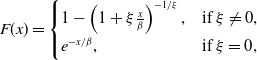 \begin{equation*} F(x)= \begin{cases} 1-\left(1+\xi\frac{x}{\beta}\right)^{-1/\xi},&\mbox{if $\xi\neq 0$}, \\ e^{-x/\beta}, & \mbox{if $\xi= 0$}, \end{cases}\end{equation*}
where $x\in[0,\infty)$
if
$x\in[0,\infty)$
if $\xi\ge 0$
and
$\xi\ge 0$
and $x\in[0,-\beta/\xi)$
if
$x\in[0,-\beta/\xi)$
if $\xi\lt 0$
. By the Pickands-Balkema-de Haan Theorem (Balkema and de Haan, Reference Balkema and de Haan1974; Pickands, Reference Pickands1975), the generalized Pareto distributions are the only possible nondegenerate-limiting distributions of the excess of random variables beyond a high threshold. If
$\xi\lt 0$
. By the Pickands-Balkema-de Haan Theorem (Balkema and de Haan, Reference Balkema and de Haan1974; Pickands, Reference Pickands1975), the generalized Pareto distributions are the only possible nondegenerate-limiting distributions of the excess of random variables beyond a high threshold. If $\xi\ge 1$
,
$\xi\ge 1$
, $F\in\mathcal{H}$
. This is by Proposition 2 (iv); that is, the generalized Pareto random variables with
$F\in\mathcal{H}$
. This is by Proposition 2 (iv); that is, the generalized Pareto random variables with $\xi\ge 1$
can be obtained from location-scale transforms of Pareto
$\xi\ge 1$
can be obtained from location-scale transforms of Pareto $(1/\xi)$
random variables.
$(1/\xi)$
random variables.
Example A.3 (Burr distribution). For $\alpha,\tau\gt 0$
, the Burr distribution is defined as
$\alpha,\tau\gt 0$
, the Burr distribution is defined as
 \begin{equation}F(x)=1-\left(\frac{1}{x^\tau+1}\right)^\alpha, x\gt 0.\end{equation}
Let $Y\sim\textrm{Pareto}(\alpha)$
. Then
$Y\sim\textrm{Pareto}(\alpha)$
. Then $Y^{1/\tau}$
follows a Burr distribution. If
$Y^{1/\tau}$
follows a Burr distribution. If $\alpha,\tau\le1$
, the Burr distribution is super-Pareto and hence
$\alpha,\tau\le1$
, the Burr distribution is super-Pareto and hence $F\in\mathcal{H}$
. Special cases of Burr distributions are the paralogistic (
$F\in\mathcal{H}$
. Special cases of Burr distributions are the paralogistic ( $\alpha=\tau$
) and the log-logistic (
$\alpha=\tau$
) and the log-logistic ( $\alpha=1$
) distributions; see Kleiber and Kotz (Reference Kleiber and Kotz2003) and Klugman et al. (Reference Klugman, Panjer and Willmot2012).
$\alpha=1$
) distributions; see Kleiber and Kotz (Reference Kleiber and Kotz2003) and Klugman et al. (Reference Klugman, Panjer and Willmot2012).
Example A.4 (Inverse Burr distribution). Suppose that Y follows the Burr distribution (C1). Then $X=1/Y$
follows the inverse Burr distribution
$X=1/Y$
follows the inverse Burr distribution
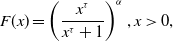 \begin{equation*}F(x)=\left(\frac{x^\tau}{x^\tau+1}\right)^\alpha, x\gt 0,\end{equation*}
where $\alpha,\tau\gt 0$
. If
$\alpha,\tau\gt 0$
. If $\tau\le 1$
, it is easy to check that the second derivative of
$\tau\le 1$
, it is easy to check that the second derivative of $h_F$
is always negative, and thus
$h_F$
is always negative, and thus $h_F$
is subadditive. Hence
$h_F$
is subadditive. Hence $F\in\mathcal{H}$
if
$F\in\mathcal{H}$
if $\tau\le 1$
. Note that the property of
$\tau\le 1$
. Note that the property of $\mathcal{H}$
may not always be preserved under the inverse transformation. For instance, if Z follows a Fréchet distribution without finite mean, then
$\mathcal{H}$
may not always be preserved under the inverse transformation. For instance, if Z follows a Fréchet distribution without finite mean, then $1/Z$
follows a Weibull distribution whose mean is always finite.
$1/Z$
follows a Weibull distribution whose mean is always finite.
Example A.5 (Log-Pareto distribution). If $Y\sim \mathrm{Pareto}(\alpha)$
,
$Y\sim \mathrm{Pareto}(\alpha)$
, $\alpha\gt 0$
, then
$\alpha\gt 0$
, then $X=\exp(Y)-1$
has a log-Pareto distribution (see p. 39 in Arnold, Reference Arnold2015), with distribution function
$X=\exp(Y)-1$
has a log-Pareto distribution (see p. 39 in Arnold, Reference Arnold2015), with distribution function
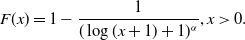 \begin{align*}F(x)=1-\frac{1}{(\log(x+1)+1)^\alpha}, x\gt 0.\end{align*}
If $\alpha\in(0,1]$
, by Proposition 2 (iv),
$\alpha\in(0,1]$
, by Proposition 2 (iv), $F\in\mathcal{H}$
.
$F\in\mathcal{H}$
.
Example A.6 (Stoppa distribution). For $\alpha\gt 0$
and
$\alpha\gt 0$
and $\beta\gt 0$
, a (location-shifted) Stoppa distribution can be defined as
$\beta\gt 0$
, a (location-shifted) Stoppa distribution can be defined as
 \begin{equation*}F(x)=\left(1-\frac{1}{(x+1)^\alpha}\right)^\beta, x\gt 0.\end{equation*}
Since a Stoppa distribution is a power transform of a Pareto distribution, by Proposition 2 (ii), if $\alpha\le 1$
,
$\alpha\le 1$
, $F\in\mathcal{H}$
. Power transforms have also been used to generalize Burr distributions (see p. 211 of Kleiber and Kotz, Reference Kleiber and Kotz2003).
$F\in\mathcal{H}$
. Power transforms have also been used to generalize Burr distributions (see p. 211 of Kleiber and Kotz, Reference Kleiber and Kotz2003).


 Open access