Workplace Networks and Political Selection

Abstract

Do social networks at workplaces function as cues into the political arena? We consider this question using the case of Sweden, which has many leisure politicians who work in the regular labour market. Restricting our networks to small cells of individuals within the same occupation and workplace, we find that an individual is more likely to become a politician in the future if that person has a colleague who was a politician. We further find that these newly enrolled individuals are placed higher up on the party lists – which to a very large extent dictates which party nominees are elected – in subsequent elections. Our mechanism analysis indicates that the effect is stronger if we consider political party bloc networks and that high-ability party officials are more prominent than low-ability officials in terms of recruiting from their workplace networks.

Introduction

Since the pioneering work of Lazarfeld et al. (1944), the social dimension of politics has been recognized as a potent factor that helps explain political participation. The choice to participate is, according to this sociological model, dependent on the political behaviour of those occupying one’s immediate surroundings, for example, the family or one’s neighbours (Huckfeldt and Sprague 1995). It follows that two individuals with similar personal characteristics could vary in their degree of political participation depending on where and with whom they spend their time (La Due Lake and Huckfeldt 1998). Ultimately, varying access to different social contexts can create inequalities in the degree of political participation within the electorate (for example, Lijphart 1997).

The earlier literature on the social dimension of politics has foremost been focused on the family (for example, Jennings 2007) and the neighbourhood (for example, Bratsberg et al. 2021; Cho et al. 2006; Gay 2012). In this paper, we focus instead on the workplace and ask whether social connections formed at work affect political involvement in terms of running for office in Sweden. We also investigate the intermediate mechanisms in terms of which party a person runs for and whether recruitment into politics follows ability lines at the workplace (for example, Besley 2005).

From a theoretical point of view, the workplace is an intriguing arena where people have interactions with other adults on a daily basis. Also, as argued by Mutz and Mondak (2006), the workplace, as opposed to the neighbourhood or the family, seems particularly well-suited for cross-cutting political discussions. Furthermore, many politicians with power over public policy are leisure-time politicians who are employed at regular workplaces while at the same time being politically active when not on the job. This is true for Sweden but also elsewhere. Hence, the workplace is not distinct from the political sector; rather, it can function as an arena for screening, engaging, and recruiting new candidates. In terms of selection, earlier theoretical papers have focused on the connection between the political sector on the one hand and the labour market on the other (Mattozzi and Merlo 2008). It has, for example, been hypothesized that there will be a negative selection of bad politicians who have a comparative disadvantage on the regular labour market (Caselli and Morelli 2004; Messner and Polborn 2004).

Despite the workplace being an intriguing and potentially common social arena for politics, empirical studies considering the effect of workplace connections on political candidacy remain limited. One reason for the scarce number of publications dealing with political selection and the workplace is the data requirements. To make inferences about how an individual decision is formed in a workplace context, we require detailed workplace and political candidate information for workers at a large number of workplaces over time, which is rarely available to researchers. As we have access to longitudinal Swedish administrate data with these features, we use it to increase our understanding of the workplace as a context that spurs political candidacy.

Because we focus on workplaces, which are inherently adult environments, it follows that we also study socialization in adulthood. Papers that have focused on adult contexts have, above all, investigated the neighbourhood and then specifically voter turnout as an outcome (Bratsberg et al. 2021; Cho et al. 2006; Gay 2012). There is also a discussion about to what extent individuals are indeed socialized in adulthood. Campbell et al. (1980) argue that individuals become increasingly frozen in their political behaviours and opinions as they become older. From a normative standpoint, we argue it would be reassuring if political engagement could be affected by the social surroundings after a person has left the parental nest. After all, it is adults who are politicians and not children.

We arrive at three main conclusions. First, we find evidence that having a political colleague increases one’s probability of becoming a politician in the future. On average, an increase of one politician among ten colleagues increases the tendency to run for office in the next term by approximately 12 per cent relative to the average tendency to run for office. Second, Swedish elections largely operate through party lists in which different parties rank their candidates locally, regionally, or nationally. Most voters vote for a party rather than for a specific candidate. Consequently, the ranking of a particular nominee on the party lists, as chosen by the parties, directly influences who gets elected. Our results show that workplace networks on average cause nominations at a lower relative ranking position, but the nominated have a better rank on the party list already within a single mandate period. In other words, workplace networks increase the tendency to be nominated for office in the short term, and those nominated are placed higher on the party lists in subsequent mandate periods. Third, the mechanism behind the main effect is, first and foremost, partisan. Individuals with left-wing politician colleagues at work are more likely to become (left-wing) nominated politicians themselves, and the same goes for their right-wing counterparts. We also find some evidence for an inbreeding bias: high-ability individuals are more likely to become politicians if they have politician colleagues who are also of high ability (although high-ability politicians recruit both high- and low-ability colleagues).

We identify the effect of having politician colleagues upon one’s entry into politics by using Swedish full-population data from 2002–2018. Our data allows us to pinpoint smaller cells of colleagues who are likely to have social interactions on a daily basis. The primary identification strategy relies on individual and workplace/occupation fixed effects, where we make use of the timing of entry into politics among those individuals who eventually become a politician at some point. The identification is derived from future nominations of workers who stay within the same workplace and occupation in which the share of nominated politicians changes over time – primarily because a nominated politician enters or drops out of the workplace. As this strategy solves most, but not necessarily all problems connected to endogenous sorting, we complement our main analysis using i) a dynamic event study, ii) placebo estimations, and iii) a battery of sensitivity checks. The empirical design is explained in detail in Section 4.

We contribute with new results to the massive literature on political socialization. ¹ Scholars have taken an interest in the relationship between social networks and political participation, but their focus has generally been on strong ties or the neighbourhood context. A couple of papers, though, do focus on workplaces. Using Swedish survey panel data, Adman (2008) tests whether workers who are employed at a workplace where decision making is more democratic have a higher rate of political participation, and he finds no support for this claim. Mutz (2002) argues that being part of a network may lower the level of political participation if people within the network (such as co-workers) have conflicting political views. These questions are related to the discussion on whether strong social networks, such as families (wherein people are more similar to each other), have a greater impact on the political behaviour of individuals than do weak social networks (wherein people are more likely to encounter heterogeneous political opinions). Focusing on outcomes such as contacting officials, protest activities, or whether respondents were involved in community politics, Lim (2008) investigated different types of social ties (including workplace ties) using American data from the Citizen Participation Study. Lim (2008) concludes that weak ties may be just as important as strong ties when it comes to engaging new activists in politics. Folke et al. (2025) demonstrate, using registry data, that Swedish politicians have varying occupations and that their labour market experience is associated with their future ideological position along the economic left/right dimension and the libertarian/authoritarian spectrum. Their paper provides an empirical test of the theory presented in Kitschelt (1994) on the labour market foundations of party choice. Our paper relates to this discussion, but our focus is, instead, on labour market networks, not on specific occupations or workplaces. ²

There is also emerging literature on workplace ties and their effects on future political careers, but in which the evidence originates from non-democratic settings. Fisman et al. (2020) analyze promotions to the Politburo within the Chinese Communist Party and test whether a person is more likely to become a member if he or she had an earlier workplace connection, school connection, or hometown connection with a member who is retiring. The authors find no effect from workplace connections, and they find negative effects from school and hometown connections, which they interpret as indicative of competition within fractions of the Chinese Communist Party. However, Jia et al. (2015) find that provincial leaders are more likely to be promoted if they had an earlier workplace connection within the central government and if they have also delivered economic growth in their district. Our paper contributes to this literature but with empirical evidence from a democratic country where the incentives and rules are quite different.

Finally, a note on what we believe is a trade-off with the data and method we apply. On the one hand, full population administrative data have the advantage of including all workplaces in Sweden. We therefore do not have to limit our analyses to a given type of workplace or sector, improving generalizability. On the other hand, our data is not particularly informative on motives, opinions, and who is doing the actual recruiting. Thus, while our administrative data have many strengths, they also hold certain weaknesses which will limit our ability to flesh out the exact mechanisms.

Theoretical Framework and Mechanisms at Play

According to the civic voluntarism model (CVM) (Verba et al. 1995), there are three factors that influence political candidacy: personal resources, political attitudes, and networks to others who are already politicians. Verba et al. (1995) means that these three factors boil down to a simple rule. Simply put, the most likely reasons for people not to be involved in politics are because “they can’t, because they don’t want to, or because nobody asked” (Verba et al. 1995, 5). In this paper, we are focusing on the first and the third factor of the CVM, which we chose to denote as the supply and the demand side of workplace political engagement. We connect the CVM to related theoretical models, which together provide a useful discussion regarding the intermediate mechanisms between workplaces and running for office.

Personal Resources: Supply Side

Information and encouragement at the workplace from already active politicians may increase a person’s resources, which, in turn, may tip the person over to political engagement. Moreover, in addition to helping reduce information costs, a politician colleague may create a socialization environment for political engagement. This may take the form of political discussions that foster interest among those not already politically engaged. Connecting to the idea of social capital (for example, Putnam et al. 2000), the social activities at the workplace can increase social capital through everyday political discussions in line with the idea in La Due Lake and Huckfeldt (1998). Such personal acquaintances can provide the necessary information about that person’s party, and enrollment in the party may then take place without any process of active recruitment. However, the workplace politician in question may also furnish general information about political engagement, thereby lowering the cost of information-gathering on a more general level. In that case, having a politician colleague may increase one’s likelihood of becoming a candidate for any party – not necessarily that of one’s colleague.

It is a fact that only a small part of the population runs for political office. In order to understand why a person makes the effort to run for office – instead of just settling for voting for a specific candidate – it is also fruitful to think about the incentives for entry into politics. One way of modelling entry is offered by the first step in the seminal citizen-candidate model (CCM) presented in Osborne and Slivinski (1996) and Besley and Coate (1997), according to which people become candidates if doing so maximizes their utility. This part of the CCM may be related to the personal resource factor in the CVM. According to the CCM, the choice to run for office is endogenous: it depends on the policy positions of other candidates, their ability to enact said policies, and on the costs of entry. Costs of entry include the costs incurred in gathering information on the different parties and establishing contacts with persons who are already politically engaged. Politician colleagues would lower such entry costs and thus increase the supply of politicians from workplaces relative to other social arenas.

Demand Side

In addition to affecting entry costs, the workplace can function as a recruitment arena where people are being asked to join a specific party.

To illustrate this mechanism, let us assume the existence of political parties with the objective function of seeking to win elections and to govern. These parties consist of party members, who are essentially citizens, some of whom have decided to run for office. The party members, however, differ in their capacity. We interpret capacity in terms of political ability, by which we mean gaining votes in elections and being a productive legislator. In practice, however, we shall assume that political ability is a function of (and is well approximated by) some measure of innate ability and overall human capital.

Since the parties cannot directly observe the political ability of non-member citizens, there is information asymmetry. From the parties’ point of view, all potential new party members are observationally equivalent. Yet, the parties must decide whether to nominate new members to political office – before observing their political ability.

In line with the seminal labour-economics model set out by Montgomery (1991), we argue there is an inbreeding bias among colleagues, whereby high-ability workers are likely to have stronger social ties with other high-ability workers than with their low-ability colleagues. Simply put, individuals at work socialize with others who are like themselves. Because of this, parties maximize their utility by recruiting on the basis of referrals from high-ability party members since the latter are more likely to know other people of high ability. In this sense, workplace networks function as a selection mechanism for new party officials.

This line of thought closely recalls the argument presented by Brady et al. (1999), who model the recruitment of political activists. They argue that politicians have an incentive to gather information on activists’ potential (that is, their ability). Brady et al. (1999) contend further that recruiters have an incentive to use cues to ascertain the political potential of prospective members. The use of referrals from already-party members can be seen as a way of screening political candidates informally. The earlier literature on candidate selection has emphasized that contact capital and informal rules need to be taken into account if we are to understand why certain individuals are deemed suitable as candidates by the parties (Widenstjerna 2020).

Although the main channel should be that high ability party members recruit other high ability individuals from their workplace networks, it bears noting that Mattozzi and Merlo (2015) discuss an equilibrium where political parties in a proportional representation system (where political competition is lower) recruit new officials that are mediocre, but more homogeneous, because parties need such members for organizational reasons. Such mediocre members have less profitable outside options in comparison to high-ability members, according to this model.

Demand Side or Supply Side?

Two of the important features discussed above are the extent to which a newly nominated candidate as well as the relevant politician colleague are of the same party and of similar ability. These features would fit nicely with a story of active recruitment, whereby a party recruit by referrals. As both partisanship and ability are matters we observe (or can approximate well) we will show evidence on these features in the upcoming analyses. The idea is that such analyses will shed some – albeit suggestive – evidence on the mechanisms at play

Despite the very detailed data, it remains difficult to separate the importance of entry costs from active recruitment, and we will not be able to fully isolate the importance of supply and demand factors. In the unlikely case in which we find that a politician colleague matters almost only for the probability of becoming a candidate for another party than the one represented by one’s co-worker, we may actually rule out a demand-side recruitment mechanism. But, if we find that having a politician colleague both increases the probability of running for the same party as one’s co-worker for some individuals and increases the probability of running for the opposition for others, we end up in a more complicated scenario. In this case, we need to turn to our previous discussion on inbreeding bias, in line with Montgomery (1991). If we find no evidence of an inbreeding bias, we argue that a demand-driven mechanism is less likely to be operating since such a channel presupposes that parties try to recruit by referrals. On the other hand, if we find support for an inbreeding bias, we at least cannot rule out a demand-side mechanism. The latter conclusion is also valid if we find inbreeding bias and purely partisan effects.

Institutional Background

Swedish Case

In 2018, 77 per cent of all females and 80 per cent of all males aged 16 to 64 were employed in Sweden (SCB 2018). Thus, a large part of the Swedish population spends a considerable amount of time at a workplace. This mere fact makes the workplace context important to study as an arena of political engagement. We have access to merged individual and workplace data (anonymized). We also have information on individuals’ occupations. These features enable us to pinpoint small cells of colleagues who are likely to spend time together.

Party System in Sweden

We study elections in Sweden. Elections for three different levels of government take place every fourth year on a single day. These levels of government are often referred to as the national, regional, and local levels, and the corresponding elections are to the parliament, the county councils, and the municipalities. A person needs to be 18 or older to vote and to run in an election. Local and regional politicians have a substantial say over economic policy. For example, municipalities in Sweden have the right to set their own tax rates, and they are important providers of welfare services. The regions, too, have the right to collect taxes, and they are primarily responsible for the publicly funded health-care system. Eight parties are represented in the Swedish parliament: the Left Party, the Social Democrats, and the Green Party, which together are considered to form the left-wing bloc; and the Center Party, the Liberal Party, the Christian Democrats, and the Moderates (conservatives), which traditionally form the right-wing bloc. Then there are the Sweden Democrats, who entered the parliament in 2010. This party has not been included historically in either of the two traditional blocs. In recent years, however, it has steadily positioned itself as a right-wing anti-immigration party. As a consequence, the traditional bloc division between left and right has faded in Swedish politics after 2010, mainly due to the emergence of the Sweden Democrats.

Lists and Party Nomination Process

Elections are held with a flexible-list PR system. Political parties first rank their candidates on local, regional, and national lists, which are in turn put forward to the voters. A candidate’s position on the party list is the most important factor in terms of their chances of getting elected because it determines – together with the vote share for the party – which candidates on the list obtain a seat. Voters can also cast a personal preference vote, but it is unusual for a candidate to be elected only through personal votes from an otherwise insufficient list position. Those on the list who are not elected become substitutes for the elected candidates, and it is also common for substitutes to serve on various subcommittees (nämnder). Since the list position of a candidate is crucial, the process by which the composition of the party list is determined is of high relevance. Widenstjerna (2020) studied the Swedish nomination process in great detail by interviewing key figures within the parties. Drawing on his work, we can conclude at least three stylized facts about the process. First, there is no law on party nomination processes, consequently, the process varies between parties. Some use primaries, others decide by local boards. Second, while variation across parties is evident, most or all party lists are first suggested by election committees. It is therefore safe to say that the composition of the election committees will matter in terms of chosen nominees. We do not, however, have any information on specific committee positions held by party figures. Finally, much like hypothesized in this article, the respondents in the study by Widenstjerna (2020) confirmed the perceived importance of contact capital (such as, for example, a workplace connection). It is beneficial for potential new nominees to know respected figures within the party, as it will reflect well on the suggested candidates themselves. ³

Beyond the specifics of the Swedish process, an additional issue for parties when choosing candidates is descriptive representation. To gain votes, parties may act strategically and choose candidates that represent different demographic groups or localities (Fiva et al. 2021). Possibly, this could also apply to occupations, whereby individuals from certain professions are recruited strategically. ⁴

Data and Empirical Model

Empirical Universe

In our panel, which is based on data from Swedish administrative registers, the first year is 1998, and the last one is 2018. The minimum age for standing as a candidate in Sweden is 18, and most Swedes retire before age 67: 18–67 is thus the age span for the individuals included since we need to have information on whether they are candidates as well as particulars on their occupation and place of work. Also, since our panel estimations make use of information specific to occupations and workplaces over time, we require an individual to be employed at a registered workplace with a corresponding occupation throughout our panel. For the first mandate period (1998–2002), we use occupation and workplace codes from the last year in the mandate period (2001) because we do not have access to accurate occupation codes for earlier years. More details regarding the data sample are found in Section A2 in the Appendix.

Outcome Variable

The focus of our main analysis is on nominated politicians: that is all individuals who have ever run for a municipal council, a county council, or the national parliament. The outcome variable is defined as a dummy variable, which is equal to 1 if the person is nominated in a given mandate period and 0 otherwise. Note also that we have a strong prior here – that there is a considerable incumbency advantage in politics. We therefore restrict our main analysis to individuals in the panel who have not themselves been nominated previously.

Treatment Variable: Workplace-Occupation Networks

To increase the likelihood of individuals actually having interacted with each other, we use the share of nominated politicians at the same workplace and occupation. A workplace is defined in our data as a property or address within the same firm, so it is smaller than the average size of a company. The median workplace has around forty-five employees; however, the number varies from just a few to several hundred or (in a few cases) several thousand. Furthermore, we expect many workplaces not to be vertically integrated. We therefore employ International Standard Classification of Occupation (ISCO) codes. We use 3-digit codes, which classify workers into different occupational categories.

Descriptive Statistics and Definition of Core Variables

In Table 1, we present descriptive statistics with regard to the outcome and treatment variables as well as the number of colleagues within a workplace-occupation cell.

Table 1. Descriptive statistics for core variables

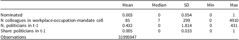
Note: Descriptive statistics for the data sample used in the analysis.

Table 1 highlights an important pattern, namely, that few individuals in absolute numbers end up being politicians. In our data sample, 0.3 percent of all individuals are nominated in a given time period (row 1). There are, on average, 0.4 politicians within a workplace-occupation cell (row 3), and the share of politicians is 0.005 among the individuals within a workplace-occupation cell (row 4). This is not surprising but a key feature of a representative democracy. However, it bears noting that for the large majority of the individuals, there are no politician colleagues in any time period, meaning that the distribution of the independent variable is very skewed in both absolute and relative numbers. Future interpretation of the estimated coefficients needs to take this into account, meaning that a small estimated coefficient could still be large relative to the mean value of the dependent variable.

The median size of the workplace-occupation cell is seven, with a mean of eighty-five colleagues (this number concerns all other colleagues except the individual in question). The difference between the median and mean is due to the fact that there are some large workplaces in our data where almost all workers have the same occupation.

With this distribution of the data in mind, we choose to scale the treatment variable as the number of politicians per ten colleagues. The reasons are multifold: first, it is transparent and makes the regression estimates easy to interpret; second, the scaling is close to the median size of the number of colleagues within a workplace-occupation cell (seven colleagues in median); third, it makes sense from a theoretical viewpoint. Both a supply and demand side explanation for political selection at work hinges on social interactions, and it seems reasonable to interpret the effects in terms of having one out of ten colleagues who is a politician. We show the full distribution of the treatment variable in the Appendix (Figure A1).

For a given individual, we calculate that person’s share of politician colleagues among ten colleagues excluding him/herself, such that the explanatory variable represents the share of politicians among the other colleagues within the same cell. If the individual later becomes a politician, he or she remains in the panel and thereby increases the share of politician colleagues for the other workers in the same cell. However, as mentioned earlier in this section, we restrict all regressions to those persons in the panel who have not been nominated previously. In practice, this means there are no individual cascade effects where an increased share due to an individual becoming a politician oneself increases the probability that one will remain a nominated politician in the future. It does mean, however, that the treatment variable is increased for the other individuals within the cell who are not yet nominated politicians.

Before we move on to our identification strategy, we want to provide a first descriptive glimpse of the relationship between the probability of being nominated and having politician colleagues. In Figure 1, we have plotted the probability of being nominated in $t$ , depending on whether there are 0 politicians at the workplace and occupation, or at least 1 in time period $t - 1$ . It is clear from Figure 0 that there is a substantial descriptive difference between these two groups, which decreases slightly over time. This provides an interesting starting point for our causal analysis later.

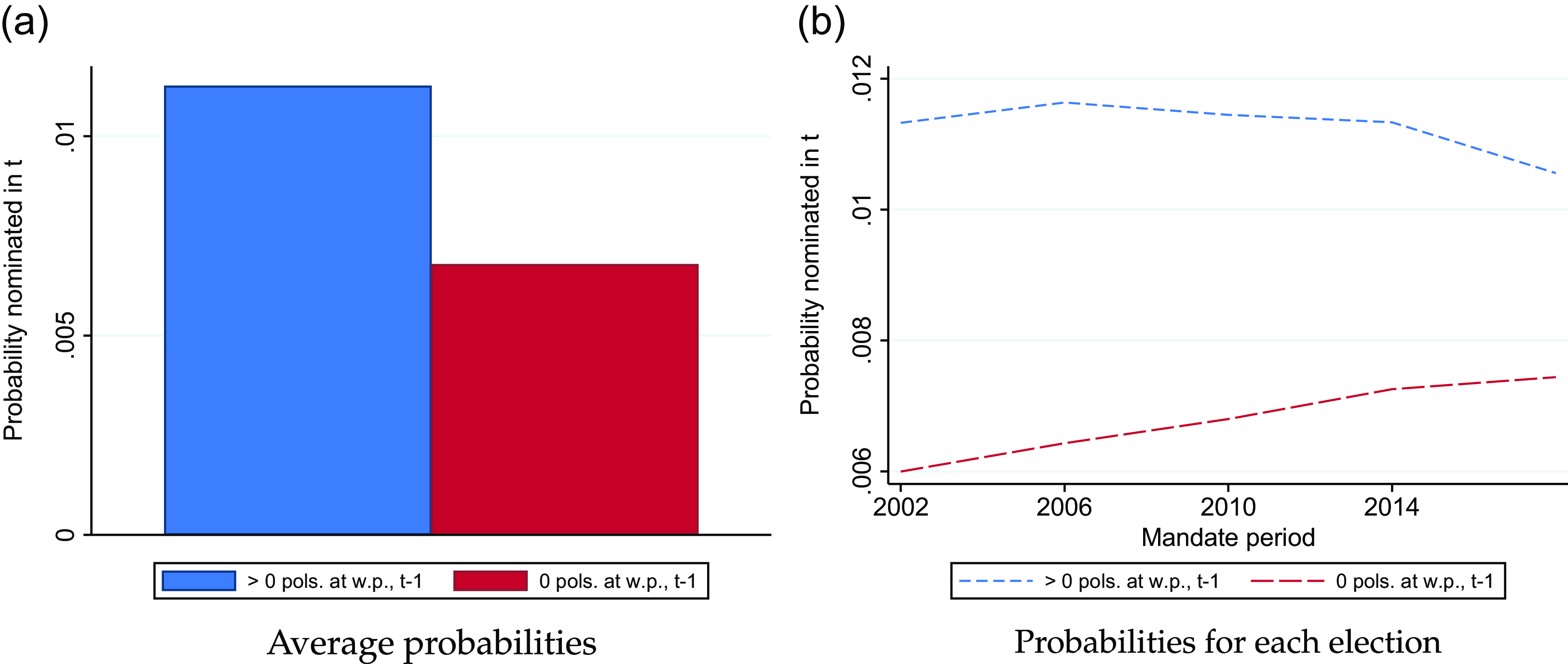
Figure 1. The probability of being nominated depends on having colleagues who are politicians.

Notes: The figures display the difference in the probability of being nominated in time period t, depending on whether one has politician colleagues in t-1 or not.

Identification Strategy and Regression Equation

In general, we believe it is reasonable to assume that selection into workplaces is less prominent than selection into other social networks, such as friends or neighbourhoods. Nevertheless, as we do not randomly allocate politicians across workplaces, there is still a possibility that the treatment (of politician colleagues) is partially determined by factors we cannot measure, which, in turn, may correlate or affect the tendency to run for office (Fox and Lawless 2005).

Our strategy for the main analysis is related to that of Cornelissen et al. (2017), who used a multitude of fixed effects and trend variables to study workplace peer effects. While the outcome of interest in their case was wages and the treatment was workplace peer quality, many of the obstacles regarding endogeneity – for example, the selection of certain individuals into specific workplaces – were shared between the two settings.

We estimate the following linear probability model in our main analysis:

(1) $$No{m_{itwom}} = {\beta _0} + {\beta _1}{X_{t - 1,wo}} + {W_{iwo}} + {\beta _2}{Z_{it}} + {\beta _3}{E_{t - 1,wo}}$$

$$+ {\tau _t} + {\phi _{w,t}} + {\varepsilon _{ot}} + {M_m} + {u_{itwom}}$$

where subscripts include $i$ for individual, $t$ for mandate time period, $w$ for workplace, $o$ for occupation, and $m$ for municipality of residence. $No{m_{itwom}}$ , the dependent variable is a dummy variable, taking the value of 1 if an individual becomes a nominated politician in $t$ , and 0 otherwise. ${X_{t - 1,wo}}$ is the treatment variable measuring the share of politicians among ten colleagues at the workplace within an occupational category (3-digit ISCO codes) in $t - 1$ . ${u_{itwom}}$ is the error term. Standard errors are clustered at the individual workplace/occupation level.

In our most restrictive specification, we further include: (i) ${E_{t - 1,wo}}$ , which is a vector consisting of the means for individuals in the workplace/occupation cell in $t - 1$ for years of education, share of females, share of immigrants, and average income level among the colleagues; (ii) ${\varepsilon _{ot}}$ , which captures occupation time trends; and (iii) ${\phi _{wt}}$ , which measures workplace time trends: (ii) and (iii) compensate for the fact that certain occupations or workplaces attract more politicians over time. At the individual level, we include ${Z_{it}}$ , a vector of time-changing individual covariates, such as years of education and standardized income for the individual in time period $t$ . We furthermore include mandate period-fixed effects ${\tau _t}$ , so as to compensate for general time differences in the probability of becoming a politician. We also include municipality-fixed effects for the municipality of residence, ${M_m}$ , because the likelihood of being nominated varies across Sweden.

Finally, and most importantly, ${W_{iwo}}$ is a grouped individual-, workplace-, and occupation-fixed effect. By including this fixed effect, we restrict the empirical analysis to individuals who work at a specific workplace in a specific occupation. This means that the identification is derived from workers who stay within the same cell of a workplace and occupation in which the share of nominated politicians changes over time – primarily because a nominated politician enters or drops out. The share of politicians can also change as a result of an alteration in the overall composition of the workplace/occupation cell. For example, if the number of colleagues who are not politicians within the same cell falls, the share of politician colleagues within the same cell mechanically rises in tandem. This embodies an intuitive logic: if the share of politicians in an occupation and workplace cell increases from 1 in 7 to 1 in 3, the chances are that the workers within the same occupation and workplace cell will have more interaction with the politician colleague in question.

Identification Discussion

Formally, the identifying assumption can be written as a conditional independence assumption. Let ${{\rm{\Gamma }}_{itwom}}$ equal the right-hand side terms in Equation 0 besides the error term ( ${u_{itwom}}$ ) and the explanatory variable of interest ( ${X_{t - 1wo}}$ ). ⁵ Conditional independence requires:

$$E({u_{itwom}}|{X_{t - 1wo}},{{\bf{\Gamma }}_{itwom}}) = E({u_{itwom}}|{{\bf{\Gamma }}_{itwom}}),$$

or, in other words, that after conditioning on our control variables and the multitude of fixed effects ( ${{\rm{\Gamma }}_{itwom}}$ ), the share of politicians at the workplace and occupation is independent of any factor potentially causing entry into politics.

What are the main threats to the conditional independence assumption? We argue that there are essentially two types of selection to worry about. Firstly, notice that since we include ${W_{iwo}}$ , we do not worry about individual heterogeneity or (time-invariant) selection into a workplace and/or occupation. Rather, a given individual’s characteristics may change over time in a way that predicts both the tendency to become a politician, as well as the changing characteristics of the workplace and occupation cell. One way to partially address this is to add time-varying controls at the individual level ( ${Z_{it}}$ ). To further test for this we provide placebo tests between the share of politician colleagues and other (same-year) individual characteristics such as parental leave or disposable income. Secondly, workplace and occupation-specific trends may correlate with the tendency to be nominated, both for new politicians entering the workplace and incumbent ones who will later become nominated. As this is essentially a question of timing, we complement our analysis with a dynamic event study.

Of course, the share of politicians is bundled with other characteristics at the workplace/occupation level. As politicians are not randomly drawn from the population, this is a mechanical feature of the treatment – if the share of politician colleagues increases, other co-worker characteristics will also change. We partially address this by adding time-changing controls at the workplace/occupation level. We refer to the results for a fuller description of other robustness tests. Finally, in Section A2, the Appendix, we discuss in more detail the challenges that we face in our empirical analysis. Here, we discuss matters such as LPM v. conditional logit and the potential issue of bias in line with Nickell (1981).

Main Results

The main results are presented in Table 2. Overall, we estimate positive and statistically significant effects for all specifications in line with our hypothesis that having politician colleagues increases one’s probability of running for office in the future.

Table 2. Main results: Probability of being nominated in $t$ when one has political colleagues in $t - 1$

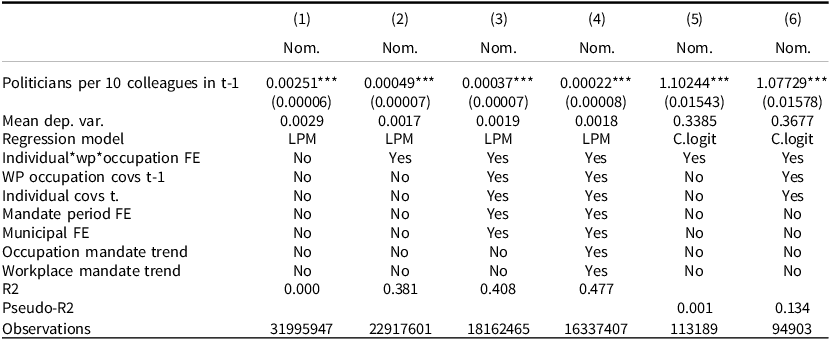
Note: Standard errors in parentheses are clustered at the individual/workplace/occupation level. *** p $ \lt $ 0.01, ** p $ \lt $ 0.05, * p $ \lt $ 0.1. The dependent variable is binary and takes the value of 0 or 1. The independent variable is the number of politicians per ten colleagues within a workplace-occupation cell. Columns 1–4 display LPM-estimated coefficients. Columns 5 and 6 present odds ratios from conditional logit models.

Column 1 in Table 2 displays the raw association between the dependent variable and the explanatory variable. In column 2 we include interacted fixed effects for individual, workplace, and occupation. Due to the inclusion of individual fixed effects, we are now, in essence, only considering the timing of actual entry into politics by the pool of persons who eventually run for office. Including fixed effects in column (2) substantially reduces the estimated coefficient, but it remains statistically significant. In column (3), we add a large number of covariates, including (i) individual covariates in $t$ (standardized income and years of education), (ii) aggregated covariates for the workplace/occupation cell in $t - 1$ (years of education, share of females, share of immigrants, and average income level among the colleagues), (iii) fixed effects for municipality of residence, and (iv) mandate period-fixed effects. In column 4, we further include workplace and occupation mandate trends. Including these fixed effects and covariates decreases the size of the estimated coefficients relative to that in column 2.

In terms of practical significance, the point estimate in the most conservative LPM specification (column 4) equals 0.00022 – meaning that when the number of politician colleagues in ten colleagues is increased by one in $t - 1$ , the probability of becoming a politician rises by $0.022$ percentage points in $t$ . This effect may appear small; however, only a small fraction of the population becomes a politician. If we divide the point estimate of $0.00022$ by the mean value of the dependent variable $\left( {0.0018} \right)$ , we find that an increase by one politician among ten colleagues increases the relative probability of becoming a politician by approximately $12.2$ percent, which must be considered as practically significant. Increasing the number of politician colleagues with one out of ten is also an intuitive increase in treatment, as it requires a median-sized workplace and occupation cell (around seven workers) to get one politician added to its staff.

The probability of becoming a politician is very different for different parts of Sweden. The main reason is the varying ratio between the number of seats in the municipal council and the size of the local population. In general, it is easier to become a politician, and the baseline probability of running for office is higher in a small municipality than in a big city. ⁶ The marginal effect is, therefore, hard to interpret – even when municipality-fixed effects are included in an LPM model – in relation to the mean of the dependent variable. As an alternative, we apply conditional logit estimations in columns 5–6. Both coefficients are statistically significant, just as in columns 1–4. In contrast to the LPM model, where all observations contribute to the estimation when there is variation on the right-hand side of the regression equation, the conditional logit model only runs on the sample where there are actual switches in the dependent variable. This is illustrated in the decrease in the number of observations in columns 5–6. A connected difference is that the LPM model includes separate intercepts for the $workplace{\rm{*}}occupation{\rm{*}}individual$ fixed effects, whereas the conditional logit models also allows for different slopes for this grouping variable.

In column (5), the coefficient equals 1.102, meaning that a positive event (becoming a politician in $t$ ) is more likely than a negative event (not becoming a politician in $t$ ) among those who eventually become politicians in the panel, if the share of politicians within the workplace/occupation cell in $t - 1$ increases by one among ten colleagues. In relative terms, this means the odds of becoming a nominated politician in the next mandate period are 10 per cent higher.

We have run several sensitivity checks to assess the robustness of the main findings in Table 2. The results are presented and discussed extensively in Section A3 of the Appendix. This includes: i) excluding certain occupations that are common in the political sphere, ii) changing the treatment variable to elected politicians, iii) running the LPM-specifications for different population sizes, iv) restricting the analysis to smaller or similar sized workplaces, v) different clustering levels of the standard errors, vi) removing outliers in the treatment variable, and, crucially, vii) placebo analyses where we change the outcome to the mandate period before the treatment window, and also investigate other labour market variables. We also present evidence against the notion that effects are only seen in a specific labour market sector.

All in all, we remain at our conclusion here in the main text after assessing these robustness analyses.

Dynamic Effects

The main estimation strategy in Table 2 has many benefits in terms of both power and isolating small cells of co-workers. However, we cannot use it to estimate the dynamic effects, that is the duration or decay of the effect. Moreover, we have discussed our results in terms of timing, but are yet to show specific direct evidence of this.

We estimate a two-way fixed effects event study (TWFE). Our outcome is defined as the change in being nominated between period $t$ and $t - 1$ . Consequently, if individual $i$ is nominated in mandate period 2 but was not nominated in period 1, the outcome is defined as 1 for mandate period 2. We define the outcome as 0 for someone who remains a (non-)politician between the two periods. The event (treatment) is the first mandate period during which a nominated politician enters the workplace and occupation cell. We require this new politician not to have worked at the workplace and occupation cell in the previous mandate period. We also require individuals in the sample to remain at the same workplace and occupation.

We then estimate the defined outcome on a set of dummies, representing mandate periods since the event. In line with the TWFE model, we include fixed effects for the individual and mandate period. We also add municipal time trends, as municipalities are widely different in their seat-to-population ratio. The control group consists of all never-treated individuals. As we believe effects are more prominent for workplace cells with fewer workers (higher chance of contact), we show one Figure with few colleagues (four to ten) and one with a larger number (ten to thirty). Note that this specification is data demanding and the sample selective.

Looking first at Figure 2a, we see suggestive evidence of an increased probability to run for office in the period after treatment. Consequently, a given individual has an increased probability of becoming a nominated politician during the mandate period following the addition of a new politician colleague at work.

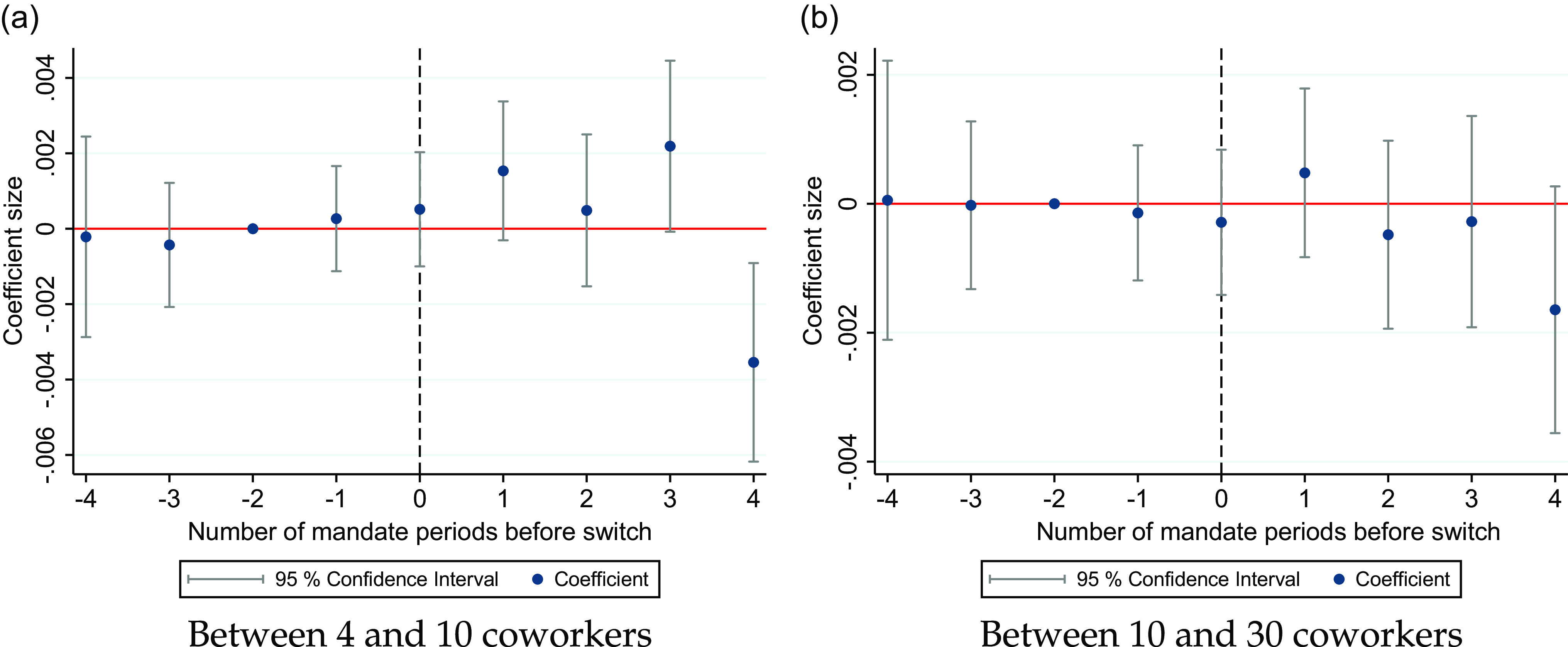
Figure 2. TWFE event study.

Notes: The figure displays the estimated coefficient and 95 per cent confidence intervals from an event study. In Figure a, we consider workplaces with between four and ten co-workers; in Figure b, between ten and thirty. See the text for more information on sample restriction. The estimation command is reghdfe, which drops singletons (Correia 2015).

We find no significant pre-treatment effects. Nevertheless, recent findings have suggested that estimating and evaluating pre-treatment effects is a heavily underpowered way to detect problems with parallel trends (Roth 2022). Hence, while we fail to find robust evidence of a significant pre-trend, we caution that this diagnostic test suffers from low power.

In terms of size, the likelihood to switch to being a nominated politician increases by 0.002, the mandate period following the event. We may compare this to the average probability among the never treated. As around 1.2 per cent of this group become a politician at any point, the relative increase is around 17 per cent, which is fairly close to the estimated relative probabilities found in the main results.

At the same time, Figure 2b shows a very small effect after treatment. We consider this not too far from expectations. Regardless of whether we think of the main mechanism being one of recruitment or a changed calculus for the already employed (better and more ready information), the story is about contact. With four to ten colleagues, day-to-day contact is almost bound to happen. This, however, is not necessarily the case for larger workplaces, which we see suggestive evidence of in Figure 2b.

A widely held critique towards the TWFE models is that estimates may be biased, largely due to treatment heterogeneity (Roth et al. 2023). Different econometricians have offered different solutions to this problem. We implement one such solution by Sun and Abraham (2021a). In practice, we implement the “eventstudyinteract” command in Stata (Sun and Abraham 2021b) and use the never treated as the control group. The results are found in Figure 3. We again divide the sample into two groups, one with four to ten co-workers and one with ten to thirty. Our overall impression is that the results look very similar to the results in Figure 2. If anything, the results with the more robust event study design suggest a more precisely estimated effect for both workplaces with four to ten colleagues as well as those with ten to thirty. ⁷

Figure 3. Event study based on Sun and Abraham (Sun and Abraham, 2021a).

Notes: The figure displays the estimated coefficient and 95 per cent confidence intervals from en event study. In Figure a, we consider workplaces with between four and ten co-workers, in Figure b, between 10 and 30. See the text for more information on sample restriction. The estimation command drops singletons.

Intensive Margin

Up until this point, we have focused on the probability of becoming a nominated politician in the next mandate period, conditional on having politician colleagues at the workplace. This is essentially an analysis along the extensive political margin. What about the intensive margin? In Section B1 in the Appendix, we provide an analysis where we investigate list position categories as outcomes. Here, we follow Buisseret et al. (2022), who divide each party nomination list in Sweden into six different categories. We run this analysis for both the next mandate period, just as in the main analysis, but also for subsequent elections.

The overall conclusion from these intensive margin analyses is that the main effect is driven by nominations in the certain loss category in $t$ . Workplace networks increase the probability of running for office; however, the main effect may be explained by lower list nominations in the next mandate period, that is, the nominated candidate will likely not be elected.

When we analyze time period $t + 1$ and $t + 2$ , the results change. Interestingly, we now find nominations further up on the party lists. A plausible interpretation of these results is that it takes some time to advance within party politics. A newly recruited party member is not immediately entrusted with a higher position, yet workplace networks can function as a first stepping stone in a political career.

That said, many other events occur during these mandate periods, and we have not pinpointed the exact mechanism for future political advancements in subsequent mandate periods. Our results suggest that workplace networks cause a higher likelihood of being nominated and that these nominated politicians later go on to climb the internal party rankings. We do, however, not say that workplace networks cause the increase in rankings on party lists.

Disentangling the Intermediate Mechanisms

Let us now return to our discussion in Section 2 on intermediate mechanisms. Let us first consider whether the positive effects in Table 2 may be explained by an increase in the probability of running for the same political bloc as one’s politician colleague.

Partisan Channel

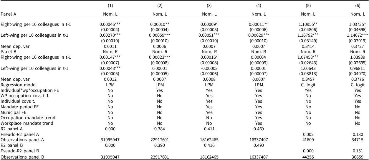
Swedish politics has historically revolved around two different blocs: a left-wing bloc and a right-wing one. Our subsequent analysis is based on the division between these two blocs. In the upper panel of Table 3, the outcome variable takes the value of 1 if the individual was nominated for a party in the left-wing bloc and 0 otherwise. In the bottom panel the outcome is similarly defined, but regarding nominations for the right-wing bloc. In both panels, we include two explanatory variables for the number of politicians per 10 colleagues belonging to the left-wing bloc and the right-wing bloc, respectively.

Table 3. Mechanism analysis: Results by left-wing and right-wing bloc

Note: Standard errors in parentheses are clustered at the individual/workplace/occupation level. *** p $ \lt $ 0.01, ** p $ \lt $ 0.05, * p $ \lt $ 0.1. The dependent variable is binary and takes the value of 0 or 1. The independent variables are the shares of right-wing and left-wing politicians among the colleagues within a workplace-occupation cell. These variables are scaled so that they represent an increase from zero to one politician among ten colleagues. Columns 1–4 display LPM-estimated coefficients. Columns 5 and 6 present odds ratios from conditional logit models.

Our overall conclusion from Panel A is that having both left-wing and right-wing politician colleagues increases one’s likelihood of being nominated for the left-wing bloc. However, in terms of size, the treatment variable for the share of left-wing politicians, representing within-partisan networks, is approximately three times larger than the estimated coefficient for the share of right-wing politicians in the most conservative LPM specification (column 4). If we perform the same exercise as we did when we discussed the main results and divide the point estimate in the most conservative LPM specification (0.00029) with the mean of the dependent variable (0.0007), we find that if the number of left-wing politicians increases by one among ten colleagues in $t - 1$ , the relative probability of becoming nominated for the left-wing bloc in $t$ is increased by 41 per cent.

The pattern emerges in Panel B for right-wing nominations too: the statistically significant coefficients are generally found for the share of right-wing politician colleagues and not for left-wing ones. In terms of size, the estimated coefficients are also larger for the share of right-wing politicians in $t - 1$ . ⁸ In terms of an increase in relative probability, we again focus on the most conservative LPM specification in column 4. It should, however, be noted that this particular point estimate is not statistically significantly different from zero, but we choose the same point of comparison as before to be consistent. If we divide the point estimate (0.00004) with the mean of the dependent variable (0.0007), we find a relative increase of being nominated for the right-wing bloc is increased by 5.7 per cent (the relative probability increase is 20 per cent in column 3).

While there seems to be some evidence that people become politically engaged for the other bloc than the one represented at the workplace, this effect is smaller and less precisely estimated than the impact that having politician colleagues has on running for the same bloc as those colleagues. All in all, these results point toward partisan political engagement at the workplace. ⁹

In the Appendix Section D1 we also run and discuss a connected heterogeneity analysis with regards to political power. We find some suggestive evidence that right-wing politicians are relatively more likely to be politically engaged when having right-wing politician colleagues when the right-wing bloc has the majority in the municipal council, but no such heterogeneous effects for political power for left-wing politician engagement.

Ability Channel

In the section on our theoretical framework, we argued that individuals with similar innate abilities socialize with each other in the workplace and that political parties are likely to recruit on the basis of referrals from high-ability party members.

We focus on cognitive ability, which is a good predictor for success in the labour market (Lindqvist and Vestman 2011). Furthermore, cognitive ability is usually viewed as a latent factor that positively affects various aspects of a person’s life. This data originates from the Swedish system of military conscription, which encompassed all men (with a few exceptions) up until 2009. A number of tests were carried out in order to sort conscripts into different military positions. One was a modified version of an IQ test, the overall goal of which was to measure the $g$ -factor. Women could enlist on a voluntary basis, but the women who chose to do so were probably not representative, so we only use the data for men. We complement the data on cognitive ability with the grade point average (GPA) from Swedish upper secondary school for women, which we argue is another proxy for cognitive ability. For cognitive ability, we standardize the measure with mean 0 and standard deviation 1 for each cohort in the data. For the GPA, we standardize the variable for each graduation cohort.

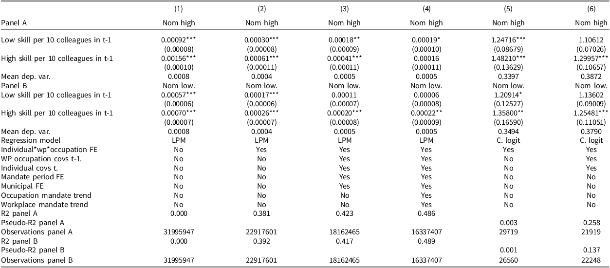
If we are to ensure that these proxies address inbreeding bias, we need to relate them to the political party that eventually ends up recruiting new members. We define a high (low) -ability variable as taking the value 1 if an individual i) is nominated by a political party and if ii) this individual’s ability is greater than (lower than) the average ability of the other nominated members within this party. Both of these variables take the value of 0 if conditions 1 and 2 are not fulfilled. ¹⁰ From these variables, we generate two treatment variables: the number of politicians among ten colleagues who are of high ability on the one hand and of low ability on the other. We then include both of these treatment variables in a split-sample analysis. The results are presented in Table 4.

Table 4. Mechanism analysis: Results by high- and low-ability politicians

Note: Standard errors in parentheses are clustered at the individual/workplace/occupation level. *** p $ \lt $ 0.01, ** p $ \lt $ 0.05, * p $ \lt $ 0.1. The dependent variable is binary and takes the value of 0 or 1. The independent variables are the shares of high-skilled and low-skilled politicians among the colleagues within a workplace-occupation cell. These variables are scaled so that they represent an increase from zero to one politician among ten colleagues. Columns 1–4 display LPM-estimated coefficients. Columns 5 and 6 present odds ratios from conditional logit models. It should be noted that the enlistment data starts in 1969, and the GPA data starts in 1973. Our mechanisms analysis is, therefore, run on a subset of the individuals from the main analysis.

The outcome in Panel A is being nominated and being of high ability. The estimated coefficients for the share of high-ability politicians at the workplace are larger than the estimated coefficients for the share of low-ability politicians across almost all specifications. In terms of economic significance, we again divide the point estimate for high-ability politicians in column 4 (0.00016) by the mean of the dependent variable (0.0005), and we find that the relative probability increase is 32 per cent.

In Panel B, the results, in part, go against our hypothesized mechanism. In this case, the outcome is being nominated and being of low ability. In all of the models, the estimated coefficients are larger for the share of high-ability politician colleagues than for the share of low-ability ones, and the relative probability increase in column 4 is 44 per cent for the number of high-ability politicians at the workplace.

The results point toward an inbreeding bias in one dimension: high-ability individuals and low-ability ones are both more likely to be nominated if there are politicians at the workplace in $t - 1$ that are of high ability. This could indicate that parties make use of referrals from high-ability party members. However, the inbreeding thesis presumes that high-ability members socialize with other high-ability workers. We also find that low-ability workers have a higher probability of being nominated in $t$ if there are high-ability politician colleagues within the workplace/occupation cell in $t - 1$ . A plausible explanation for our results is that parties consult high-ability members when recruiting and that these members, in turn, recruit both high- and low-ability members at the workplace. This could be connected to the theoretical predictions in Mattozzi and Merlo (2015), where parties need mediocre members to maximize the overall success for the party. As hypothesized in Mattozzi and Merlo (2015), this scenario is more likely in a proportional representation system where electoral competition is lower, as the one we study in this paper.

Supply-Side or Demand-Side Channel?

As is often the case with mechanism analyses, we cannot definitively conclude that a certain channel is the one and only intermediate channel. Given that our results point in part to recruitment by high-ability party members, at the least we cannot rule out that a demand-driven channel is likely to be operating. However, since we also find that the probability of running for the other bloc than the one represented by one’s politician colleague is increased (although to a lesser extent than the probability of running for the same bloc), neither can we rule out that information costs have been generally reduced – meaning that a supply-side mechanism is operating as well. The most likely explanation for our results is, therefore, that both supply- and demand-side mechanisms are in play, whereby having politicians at the workplace lowers information costs, at the same time that political parties recruit on the basis of referrals from (high ability) party members at workplaces.

Discussion and Conclusion

We find that having a workplace connection with an already active politician increases one’s probability of running for office in the future. Moreover, we find that individuals who had a workplace connection in $t - 1$ are found higher up on the party lists in subsequent elections. We have shown as well that a partisan channel is the more important selection mechanism, and that there is some evidence to suggest that political selection follows lines of ability.

These results contribute to the literature on political selection – for example, Besley (2005) – by demonstrating suggestive evidence that politicians are recruited in networks that are formed in adulthood. It is also of interest that high-ability party officials are more prominent in recruiting from their workplace networks, which has the potential of changing the composition of the pool of nominated and elected politicians. Overall, our results demonstrate that the workplace could influence the composition of the Swedish political class, the members of which are able to affect which public policies are implemented. The latter is of particular interest considering recent trends in Sweden and elsewhere, showing increased levels of socioeconomic segregation across workplaces.

If we consider the entire pool of citizens, adding a cue into politics that is not determined already at a young age is likely to broaden the sample of potential candidates as compared with a scenario where all politicians are selected from active members in political youth organizations. However, the extent to which the sample of candidates is broadened by workplace selection may depend on how citizens are otherwise recruited into politics. For example, in a context where politicians are otherwise selected from a variety of socioeconomic and occupational backgrounds, adding a selection through the workplace can potentially further sustain a breadth of backgrounds among candidates. But in a context where politicians in general are selected from for example, certain educational backgrounds, workplace selection may only act to preserve this limited breadth of backgrounds.

Furthermore, since these individuals also have a workplace connection, the conditions of working individuals are likely to become a more salient issue in policy-making in a scenario where politicians implement their preferred policy. Dal Bó et al. (2017) found that Swedish politicians are more competent than the population as a whole. However, despite this positive selection into politics, personal connections and networks may still play an important role in determining political engagement. Our overall conclusion in this paper is that this is, in fact, the case.

Finally, elections in Sweden are characterized by proportional representation and multiple people on the party lists. It is not ex-ante clear that the results put forth in this article would hold in a majority voting system with single-member districts and leisure politicians. In this case, political competition is sharper in comparison to a PR voting system. The extent to which our results do generalize in other institutional contexts is, in the end, an empirical inquiry, which only future research can answer.