The Fair Game: Auditing & debiasing AI algorithms over time

Abstract

An emerging field of AI, namely Fair Machine Learning (ML), aims to quantify different types of bias (also known as unfairness) exhibited in the predictions of ML algorithms, and to design new algorithms to mitigate them. Often, the definitions of bias used in the literature are observational, i.e. they use the input and output of a pre-trained algorithm to quantify a bias under concern. In reality, these definitions are often conflicting in nature and can only be deployed if either the ground truth is known or only in retrospect after deploying the algorithm. Thus, there is a gap between what we want Fair ML to achieve and what it does in a dynamic social environment. Hence, we propose an alternative dynamic mechanism, “Fair Game”, to assure fairness in the predictions of an ML algorithm and to adapt its predictions as the society interacts with the algorithm over time. “Fair Game” puts together an Auditor and a Debiasing algorithm in a loop around an ML algorithm. The “Fair Game” puts these two components in a loop by leveraging Reinforcement Learning (RL). RL algorithms interact with an environment to take decisions, which yields new observations (also known as data/feedback) from the environment and in turn, adapts future decisions. RL is already used in algorithms with pre-fixed long-term fairness goals. “Fair Game” provides a unique framework where the fairness goals can be adapted over time by only modifying the auditor and the different biases it quantifies. Thus, “Fair Game” aims to simulate the evolution of ethical and legal frameworks in the society by creating an auditor which sends feedback to a debiasing algorithm deployed around an ML system. This allows us to develop a flexible and adaptive-over-time framework to build Fair ML systems pre- and post-deployment.

1. Introduction

In today’s era, learning machines are at the epicentre of technological, social, economic and political developments, their continuous evaluation and alignment are critical concerns. In 2016, World Economic Forum¹ recognised the study of learning machines, i.e. machine learning (ML)(Barocas et al., 2023), and its superset artificial intelligence (AI) to be the driving force of the fourth industrial revolution.² Reckoning of modern AI not only motivates development of efficient learning algorithms to solve real-life problems but also aspires socially aligned deployment of them. This aspiration has pioneered the theoretical and algorithmic developments leading to ethical, fair, robust and privacy-preserving AI, in brief responsible AI (Dwork and Roth, 2014; Cheng et al., 2021; Liu et al., 2021; cas et al., 2023). The frontiers of responsible AI are well developed for static data distributions and models, but their extensions to dynamic environments are limited to reinforcement learning (RL) with stationary dynamics (Sutton and Barto, 2018). Concurrently, the emerging trend of regulating AI poses novel regulations and quantifiers of risks induced by AI algorithms (Annas, 2003; Voigt and Von dem Bussche, 2017; Pardau, 2018; Madiega, 2021; Dabrowski and Suska, 2022). Followed by deployment of General Data Protection Regulation (GDPR)³ in 2018 and upcoming EU AI act⁴ in 2025–26, Europe pushes the frontiers of AI regulation and propels the paradigm of algorithmic auditing.⁵ Specially, EU AI act⁶ discusses like any publicly used technology AI should undergo an audit mechanism, where we aim to understand the impacts and limitations of using this technology, and why they are caused. But these two approaches are presently unwed.

Specifically, existing responsible AI algorithms fix a property (e.g. privacy, bias, robustness) first, then the theory is built to learn with these properties, and finally algorithms are designed to achieve optimal alignment (Dwork and Roth, 2014; Liu et al., 2021; cas et al., 2023). This present approach leaves little room for the auditor feedback to be incorporated in AI algorithms except the broad design choices.

A curious case: AIRecruiter

Let us consider an AI algorithm that uses a dataset of resumes and successful recruitments to learn whether an applicant is worth recruiting or not by an organisation. Multiple platforms, such as Zoho Applicant Tracking System⁷ and LinkedIn job platform,⁸ are already used in practice. The designer would obviously want the AIRecruiter algorithm to be accurate, regulation-friendly and practically useful. To be regulation-friendly, AIRecruiter has to consider the questions of social alignment, such as privacy, bias and safety. In addition, the labour market and company’s financial situations are dynamic. Thus, the recruitment policies and the drive to achieve social alignment of AIRecruiter evolve over time. AIRecruiter demonstrates one of the many practical applications, where social alignment of an AI algorithm over time becomes imperative.

Unbiasedness (fairness): Debiasing and auditing

If AIRecruiter is trained on historical data with a dominant demography, it would typically be biased towards the “majority” and less generous to the minorities (Barocas et al., 2023). This is a common problem in many applications: gender bias against women in Amazon hiring system,⁹ economical bias against students from poorer background in Scholastic Assessment Test (SAT) score-based college admission (Kidder, 2001), racial bias against defendants of colour in the COMPAS crime recidivism prediction system (Bagaric et al., 2019), to name a few. This issue invokes the question what is the fair or unbiased way of learning best sequence of decisions and asks for conjoining ethics and AI.

Debiasing algorithms

Due to the ambiguous notions of fairness in society, researchers have proposed eclectic metrics for fairness (also called, unbiasedness) in offline and online settings (Kleine Buening et al., 2022; cas et al., 2023). Additionally, multiple algorithms are proposed to mitigate bias in predictions (Hort et al., 2024), which are mostly tailored for a given fairness metric. A few recent frameworks are proposed to analyse some group fairness metrics unitedly (Chzhen et al., 2020; Mangold et al., 2023; Ghosh et al., 2023a) but it is not clear how to leverage them for a generic and dynamic bias mitigating algorithm design.

Auditing algorithms

The existing bias auditing algorithms follow two philosophies:¹⁰ verification and estimation. Verification-based auditors aim to check whether an algorithm achieves a bias level below a desired threshold while using as small number of the data as possible (Goldwasser et al., 2021; Mutreja and Shafer, 2023). On the other hand, estimation-based auditors aim to directly estimate the bias level in the predictions of the algorithm while also being sample-efficient (Bastani et al., 2019; Ghosh et al., 2021; 2022a; Yan and Zhang, 2022; Ajarra et al., 2025). Though initial auditors used to evaluate the bias over full input data (Galhotra et al., 2017; Bellamy et al., 2019), distributional auditors have been developed to estimate bias over whole input data distribution (Yan and Zhang, 2022; Ajarra et al., 2025). Along with researchers in the community, we have developed multiple distributional auditors yielding probably approximately correct (PAC) estimations of different bias metrics while looking into a small number of samples (Figure 3). Recently, Ajarra et al., 2025 have derived lower bounds on number of samples required to estimate different metrics to propose a Fourier transform-based auditor that estimates all of the fairness metrics simultaneously. Authors also show that the auditor achieves constant manipulation proofness while scaling better than existing algorithms. This affirmatively concludes a quest for a universal and optimal bias auditors for offline algorithms.¹¹

Need for a Fair Game: Adapting to dynamics of ethics and society

Now, if a multi-national organisation uses the AIRecruiter over the years, the nature of acquired data from new job applicants suffers distribution shift over time due to world economics, labour market and other dynamics. Similarly, the regulations regarding bias also evolve from market to market and time to time. For example, ensuring gender equality in recruitment has been well argued since 1970s (Arrow, 1971), while ensuring demographic fairness through minority admissions is still under debate.

In present literature, auditors and debiasing algorithms are assumed to have static measures of bias oblivious to long-term dynamics and to be non-interactive over time. As an application acquires new data over time, updates its model, and socially acceptable ethical norms and regulations also evolve, it motivates the vision of, and a continual alignment of AI with auditor-to-alignment loop.

In this context, first, we propose the Fair Game framework (Section 3). Fair Game puts together an Auditor and a Debiasing algorithm in a loop around an ML algorithm and treats the long-term fairness as a game of an auditor that estimates a bias report and a debiasing algorithm that uses this bias report to rectify itself further. We propose an RL-based approach to realise this framework in practice.

Then, we specify a set of properties that Fair Game and its components should satisfy (Section 4).

1. (1) Data frugal: Data are the fuel of AI and often proprietary. Thus, it is hard to expect access to the complete dataset used by a large technology firm to audit its models and algorithms. Rather, often the regulations and auditing start by interacting with the software and understanding the bias induced by it. This follows access to a part of the dataset and models to audit it for rigorously. Thus, sample frugality is a fundamentally desired property of auditing algorithms. This becomes even more prominent in dynamic settings as the datasets, models and measures of bias change over time.

2. (2) Manipulation proof: As auditing is a time-consuming and often legal mechanism, one has to consider the opportunity to update models up to a certain extent in order to match the speed of fast changing AI landscape. Thus, an ideal auditor should be able to adapt to minor shifts or manipulation in the data distributions, model properties, etc. So, we aim for building an auditor which satisfies constant manipulation proofness.

3. (3) Adaptive and dynamic: While designing an auditor for debiasing AI algorithm for real-life tasks, it should interact with the environment in a dynamic way, i.e. it should adapt to correct bias measures being in dynamic environment. For example, the notion of fairness can change over time, so an auditor should be dynamic to adapt to such properties that change over time. This is central conundrum to ensure long-term fairness.

4. (4) Structured feedback: In existing auditors, we study statistically efficient auditors yielding accurate global estimates of privacy leakage, bias and instability. All the ethical conundrums are not quantifiable from observed data but are subjective. Thus, auditors might provide preferential feedback on different sub-cases of predictions (Dai et al., 2023; Conitzer et al., 2024; Xiao et al., 2024; Yu et al., 2024). Additionally, an user who leverages an AI algorithm to make an informed decision may want to the response aligned with his/her/their preferences. An auditor can help an AI algorithm to tune their responses with respect to these preference alignments.

5. (5) Stable equilibrium: The other question is the existence of a stable equilibrium in Fair Game, which is a two-player game and both the players can manipulate the other. Under fixed bias measure but under dynamic shifts of data distribution and incremental model updates, Fair Game should be able to reach a stable equilibrium between the auditor and the AI algorithm.

Before proceeding to the contributions, in Section 2, we elaborate the algorithmic background for algorithmic auditing of bias, debiasing algorithms and their limitations as the basis of Fair Game. In Section 2.4, we briefly introduce concepts of RL as it is the algorithmic foundation of Fair Game.

2. Background: Static auditing and debiasing algorithms

2.1. Learning to predict from data: Fundamentals of ML models

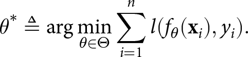
An ML model (Mohri, 2018) is a function $f: \mathcal{X} \rightarrow \mathcal{Y}$ that maps a set of input features $\mathbf{X} \in \mathcal{X}$ to an output $Y \in \mathcal{Y}$.¹² For classifiers, the output space is a finite set of classes, i.e. $\{1,\ldots,k\}$. For regressors, the output space is a d_o-dimensional space of real numbers. Training and deploying an ML model involves mainly four components: (a) training dataset, (b) model architecture, (c) loss function and (d) training algorithm.

Commonly, an ML model f is a parametric function, denoted as f_θ, with parameters $\theta \in \mathbb{R}^d$, and is trained on a training dataset D^T, i.e. a collection of n input–output pairs $\{(\mathbf{x}_i, y_i)\}_{i=1}^n$ generated from an underlying distribution $\mathcal{D}$. The exact parametric form of the ML model is dictated by the choice of model architecture, which includes a wide variety of functions over last five decades. Training implies that given a model class $\mathcal{F}=\{f_\theta|\theta\in\Theta\}$, a loss function $l: \mathcal{Y} \times \mathcal{Y} \rightarrow \mathbb{R}_{\geq0}$ and training dataset ${\mathbf{D}^T}$, we aim to find the optimal parameter

(1)\begin{align} \theta^* \triangleq \arg\min_{\theta \in \Theta} \sum_{i=1}^n l(f_{\theta}(\mathbf{x}_i), y_i). \end{align}

A loss function measures badness of predictions made by the ML model with respect to the true output. We commonly use cross entropy, i.e. $l(f_{\theta}(\mathbf{x}_i), y_i) \triangleq -y_i \log(f_{\theta}(\mathbf{x}_i))$, as the loss function for classification. For regression, we often use the square loss $l(f_{\theta}(\mathbf{x}_i), y_i) \triangleq \left( y_i - f_{\theta}(\mathbf{x}_i)\right)^2$. Finally, an optimisation algorithm is deployed to find the solution of the minimisation problem in Equation (1). We refer to the optimiser as a training algorithm.

This procedure of training an ML model is called empirical risk minimisation (ERM) (Vapnik, 1991; Györfi et al., 2006; Feldman et al., 2012; Devroye et al., 2013). ERM is at the core of successfully training decision trees to large deep neural networks, like large language models (LLMs). The key statistical concept behind using ERM to train parametric ML models is that if we have used large enough training dataset and the parametric family (aka model architecture) is expressive enough, the trained model can predict accurately (with high probability) for unseen input points coming from the same or close enough data generating distributions. This property is called generalisation ability of an ML model and is often measured with its accuracy of predictions over a test dataset. A large part of statistical learning theory is dedicated to study this property for different types of data distributions, model architectures and training algorithms (Chaudhuri et al., 2011; Dandekar et al., 2018; Mohri, 2018; Tavara et al., 2021).

In Figure 1, we provide a schematic of this training and deployment schematic of ML models in the context of AIRecruiter. Specifically, AIRecruiter uses a historical dataset of resumes and future performance of job seekers to train a recruitment predicting ML model (left side of Figure 1). After successful training of the ML model, when it is deployed in practice, a resume of a candidate is sent through it and the model recommends accepting or rejecting the candidate (right side of Figure 1). This is well known as the binary classification problem. For example, Buening et al. (2022) showed similar mechanism and its nuances of gender and demographic bias in the context of college admissions. They use 15 years of data from Norwegian college admissions and examination performances to show that the historical data and fairness-oblivious ML models trained on it exhibit different types of bias under testing. We are aware of multiple such examples worldwide, such as racial bias in crime recidivism prediction in the COMPAS case (Angwin et al., 2016), gender bias in translating and completing phrases involving occupations by LLMs (Gorti et al., 2024), economic bias in SAT score-based college admissions (Kidder, 2001) to name a few.

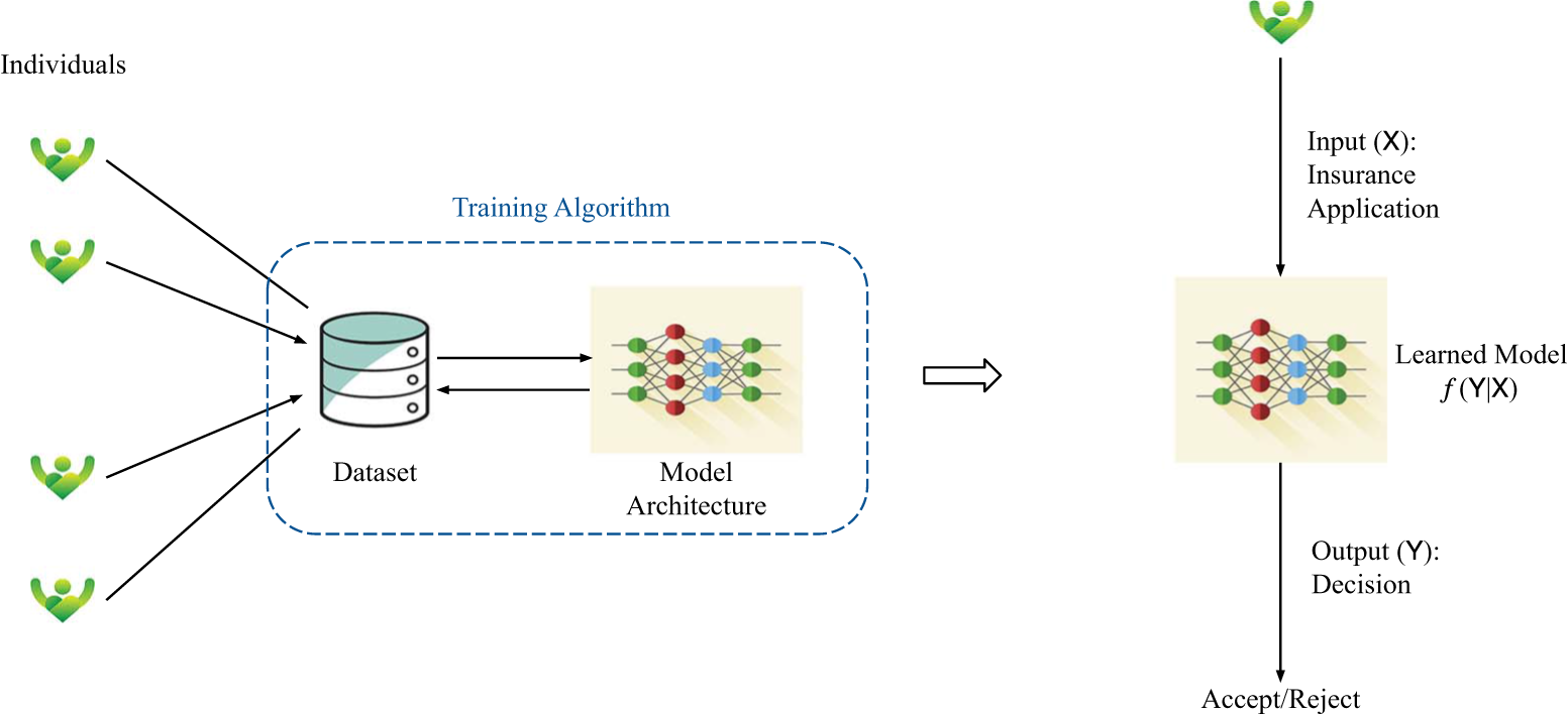
Figure 1. AIRecruiter: Training (left) and deploying (right) a machine learning model.

However, discriminations in all these cases are prohibited up to different extents by laws of different countries (Blumrosen, 1967; Fiss, 1970; Madiega, 2021; Veale and Zuiderveen Borgesius, 2021) and also are ethically unfair, in general (Novelli et al., 2023). This calls for design of bias auditing and debiasing ML algorithms.

2.2. Debiasing algorithms: State-of-the-art

A debiasing algorithm observes the input and output of an ML algorithm, the different quantifiers of bias estimated by the auditor and (if possible) the architecture of the ML algorithm to recalibrate the predictions of the ML algorithm such that the different quantifiers of bias are minimised (Lohia et al., 2019; Chouldechova and Roth, 2020; Mehrabi et al., 2021; Barocas et al., 2023; Caton and Haas, 2024).

Measures of bias

Before proceeding to the debiasing algorithms, we provide a brief but formal introduction to different measures of bias.

In order to explain measures of bias, we consider a binary classification task (e.g. AIRecruiter) on a dataset $\mathbf{D}^T$ as a collection of triples $(\mathbf{X}, \mathbf{A}, Y)$ generated from an underlying distribution $\mathcal{D}$. $\mathbf{X} \triangleq\left\{X_1, \ldots, X_{m_1}\right\}$ are non-sensitive features whereas $\mathbf{A} \triangleq\left\{A_1, \ldots, A_{m_2}\right\}$ are categorical sensitive features. $Y \in\{0,1\}$ is the binary label (or class) of ( $\mathbf{X}, \mathbf{A})$. Each non-sensitive feature X_i is sampled from a continuous probability distribution $\mathcal{X}_i$, and each sensitive feature $A_j \in\left\{0, \ldots, N_j\right\}$ is sampled from a discrete probability distribution $\mathcal{A}_j$. We use $(\mathbf{x}, \mathbf{a})$ to denote the feature-values of $(\mathbf{X}, \mathbf{A})$. For sensitive features, a valuation vector $\mathbf{a}=\left[a_1, . ., a_{m_2}\right]$ is called a compound sensitive group. For example, consider $\mathbf{A}=\{$race, sex $\}$ where race $\in\{$Asian, Color, White $\}$ and sex $\in$ $\{$female, male $\}$. Thus $\mathbf{a}=$ [Asian, female] is a compound sensitive group. We represent a binary classifier trained on the dataset D as $f:(\mathbf{X}, \mathbf{A}) \rightarrow \hat{Y}$. Here, $\hat{Y} \in\{0,1\}$ is the predicted class of $(\mathbf{X}, \mathbf{A})$.

I. Measures of independence. The prediction $\widehat{Y}$ of a classifier for an individual is independent of its sensitive feature A. Mathematically, if $\widehat{Y}$ is binary variable, independence implies that for all $\mathbf{a}, \mathbf{b}$, $\Pr[\widehat{Y}=1|\mathbf{A}=\mathbf{a}] = \Pr[\widehat{Y}=1|\mathbf{A}=\mathbf{b}]$. Statistical/demographic parity (Kamishima et al., 2012; Zemel et al., 2013; Feldman et al., 2015; Corbett-Davies et al., 2017) measures deviation from independence of a classifier for a given data distribution.

Definition 1. (Statistical parity)

$\mathrm{SP} \triangleq \max_{\mathbf{a}} \Pr[\widehat{Y}=1|\mathbf{A}=\mathbf{a}] - \min_{\mathbf{a}}\Pr[\widehat{Y}=1|\mathbf{A}=\mathbf{a}]$.

Definition 2. (Demographic parity)

$\mathrm{DP} \triangleq \frac{\min_{\mathbf{a}}\Pr[\widehat{Y}=1|\mathbf{A}=\mathbf{a}]}{\max_{\mathbf{a}}\Pr[\widehat{Y}=1|\mathbf{A}=\mathbf{a}]}$.

The use of aforementioned metrics ensures equality of outcome across demographics. However, they can lead to accepting random people from majority and qualified people from minority, due to sample size disparity.

II. Measures of sufficiency. The probability of positive outcome $\widehat{Y}$ for an individual given the true outcome is positive Y = 1 should be independent of its sensitive feature A. Mathematically, if $\widehat{Y}$ and Y are binary variables, separation (equality of opportunity or equalised odds) implies that for all $\mathbf{a}, \mathbf{b}$, $\Pr[\widehat{Y}=1|Y=1, \mathbf{A}=\mathbf{a}] = \Pr[\widehat{Y}=1|Y=1, \mathbf{A}=\mathbf{b}]$. Separation metrics measure deviation from conditional independence of a classifier for a data distribution.

Definition 3. (Equalised odds)

$\mathrm{EO} \triangleq \max_{a,b} \lvert \Pr[\widehat{Y}=1| Y=1, \mathbf{A}=\mathbf{a}] - \Pr[\widehat{Y}=1| Y=1, \mathbf{A}=\mathbf{b}] \rvert$.

Incorporating EO (Hardt et al., 2016; Pleiss et al., 2017) as a measure of bias ensures equality of outcome for eligible individuals across demographics. But on the other hand, the true outcome Y is often not known in reality.

III. Measures of calibration. A classifier prediction $\widehat{Y}$ should be calibrated such that conditional probability of the true outcome $Y=0/1$ should be independent of its sensitive feature A given the prediction being $\widehat{Y}=0/1$. Mathematically, if $\widehat{Y}$ and Y are binary variables, separation implies that for all $a, b$, $\Pr[Y=1|\widehat{Y}=1, \mathbf{A}=\mathbf{a}] = \Pr[Y=1|\widehat{Y}=1, \mathbf{A}=\mathbf{b}]$ and $\Pr[Y=1|\widehat{Y}=0, \mathbf{A}=\mathbf{a}] = \Pr[Y=1|\widehat{Y}=0, \mathbf{A}=\mathbf{b}]$.

Definition 4. (Predictive value parity (PVP))

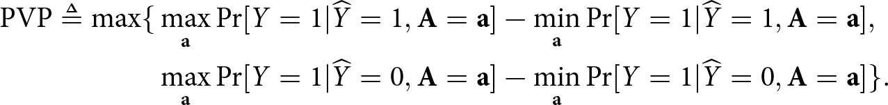\begin{align*} \mathrm{PVP} \triangleq \max \{&\max_{\mathbf{a}} \Pr[Y=1|\widehat{Y}=1, \mathbf{A}=\mathbf{a}] - \min_{\mathbf{a}} \Pr[Y=1|\widehat{Y}=1, \mathbf{A}=\mathbf{a}], \\ &\max_{\mathbf{a}} \Pr[Y=1|\widehat{Y}=0, \mathbf{A}=\mathbf{a}] - \min_{\mathbf{a}} \Pr[Y=1|\widehat{Y}=0, \mathbf{A}=\mathbf{a}] \}. \end{align*}

Such calibration measures like PVP (Hardt et al., 2016; Chouldechova, 2017) equalises chance of success given acceptance, but the acceptance largely depends on the choice of the classifier’s utility function, which can be bias inducing.

There are other causal measures of bias than these three families of observational fairness metrics. We refer to Chouldechova (2017); Mehrabi et al. (2021) and Barocas et al. (2023) for further details on them.

Debiasing algorithms

Given a measure of bias, there are three types of debiasing algorithms proposed in the literature: (a) pre-processing, (b) in-processing and (c) post-processing. These three families of algorithms intervene at three different parts of an ML model, i.e. training dataset, loss/training algorithm and final predictions post-deployment.

I. Pre-processing algorithms. These algorithms recognise that often the bias is induced from the historically biased data used for training the algorithm (Kidder, 2001; Bagaric et al., 2019; Barocas et al., 2023). When the data include a lot of samples for a demographic majority and very little for other minorities, then under ERM framework that tries to minimise the average loss to find the best parameters often lead to learning the patterns accurately for the majority and ignoring that of the minorities. Thus, pre-processing algorithms try to transform the training dataset and create a “repaired” dataset (Luong et al., 2011; Hajian and Domingo-Ferrer, 2012; Kamiran and Calders, 2012; Feldman et al., 2015; Heidari and Krause, 2018; Gordaliza et al., 2019; Salimi et al., 2019a; 2019b; 2019c). The advantage of pre-processing algorithms is that once the dataset is repaired, any model architecture and training algorithm can be used on top of it. The disadvantage is that it requires accessing and refurbishing the whole input dataset, which might include millions and billions of samples for large-scale deep neural networks. Thus, it becomes computationally intensive and requires retraining the downstream model for any update in bias measure.

II. In-processing algorithms. These algorithms aim to repair the fact that the classical ERM tries to accurately learn on an average over the whole data distribution. Thus, they either reweigh the input samples according to their sensitive features (Kamiran and Calders, 2012; Calders and Zliobaite, 2013; Jiang and Nachum, 2020) or modify the loss to maximise both fairness and accuracy (Agarwal et al., 2018; Celis et al., 2019; Chierichetti et al., 2019; Cotter et al., 2019). Some of the recent works have try and design optimisation algorithms that consider the fairness and accuracy simultaneously and iteratively during training. The advantage of these algorithms is that they achieve tightest fairness-accuracy trade-offs among the three families of debiasing algorithms. The disadvantage is that they require retraining an already established ML model from scratch, which is often time consuming, economically expensive and hard to convince the companies for whom models are central products.

III. Post-processing algorithms. The third family of debiasing algorithms approaches the problem post-training an ML model (Kleinberg et al., 2016; Chouldechova, 2017; Liu et al., 2017; 2019; Hébert-Johnson et al., 2018; Kim et al., 2018). They recognise the impact of bias of an ML model can be stopped if only the predictions can be recalibrated according to their sensitive features and corresponding input–output distributions. Thus, post-processing approaches often apply transformations to model’s output to improve fairness in predictions. If a debiasing algorithm can treat the ML model without accessing the data or training procedure, this is the only feasible approach to debias the ML model. Thus, it is the most flexible family of methods and can be used as a wrapper around existing algorithms. The only disadvantage is that we know it is not possible in one-shot to debias ML models with post-processing methods and might lead to sub-optimal accuracy levels in some cases.

For more details on the debiasing algorithms, we refer interested readers to detailed surveys and books published on this topic over years (Chouldechova and Roth, 2020; Mehrabi et al., 2021; Barocas et al., 2023; Caton and Haas, 2024).

Limitations

We do not have a framework to accommodate the bias auditor feedback to improve debiasing of the algorithm under audit. This is fundamental to bridge the regulation-based and learning-based approaches to debiasing of an ML algorithm.

2.3. Auditors of bias: State-of-the-art

An auditor looks into the input and output pairs of an ML system and tries to measure different types of bias. Any publicly used technology presently undergoes an audit mechanism, where we aim to understand the impacts and limitations of using that technology, and why they are caused. In last decade, this has slowly but increasingly motivated development of statistically efficient auditors of bias, risk and privacy leakage caused by an ML algorithm. Though the initial auditors were specific to a training dataset and used the whole dataset to compute an estimate of bias (Bellamy et al., 2018; Pentyala et al., 2022), a need of sample-efficient estimation of bias has been felt. This has led to a PAC auditor that uses a fraction of data to produce the estimates of bias which are correct for the whole input–output data distributions (Albarghouthi et al., 2017; Bastani et al., 2019; Ghosh et al., 2021; Yan and Zhang, 2022; Ghosh et al., 2022c; Ajarra et al., 2025). Here, we formally define a PAC auditor of a distributional property of an ML model, such as different bias measures.

Definition 5. (PAC auditor (Ajarra et al., 2025))

Let $\mu: \mathbf{D}^T \times f_{\theta} \rightarrow \mathbb{R}$ be a computable ¹³ distributional property of an ML model f_θ. An algorithm $\mathcal{A}$ is a PAC auditor of property µ if for any $\epsilon, \delta \in (0,1)$, there exists a function $m(\epsilon, \delta)$ such that $\forall m \geq m(\epsilon, \delta)$ samples drawn from $\mathcal{D}$, it outputs an estimate $\hat{\mu}_m$ satisfying

(2)\begin{align} \mathop{\mathbb{P}}\nolimits(|\hat{\mu}_m - \mu| \leq \epsilon) \geq 1- \delta\,. \end{align}

In Figure 2, we provide a brief taxonomy of the existing bias auditing algorithms.

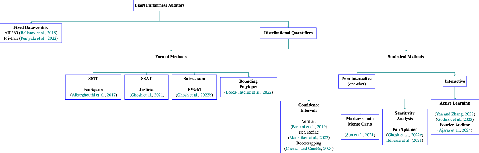
Figure 2. A taxonomy of bias auditors.

Components of a PAC auditor

As illustrated in Figure 3, any PAC auditor consists of two components: (a) sampler and (b) estimator.

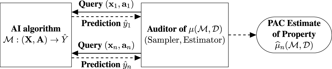
Figure 3. A generic schematic of a PAC auditor of a distributional property µ.

The sampler selects a bunch of input–output pairs from a dataset, which might or might not be same with the training dataset, and then send them further to query the ML model under audit. The information obtained by querying the algorithm depends on the access of the auditor. For example, an internal auditor of an organisation can obtain much detailed information, such as confidence of predictions, gradients of loss at the query points, etc. This is called a white-box setting. On the other hand, an external auditor (e.g. a public body or a third-party company) might get only the predictions of the ML model for the queried samples. This is called a black-box setting. Initially, the auditing algorithms used only uniformly random samples from a dataset (e.g. the “Formal Methods” and “Non-interactive” auditors in Figure 2), but we know from statistics and learning theory that uniformly random sampling is less sample efficient than active sampling methods for most of the estimation problems. Specifically, the minimum number of samples required to PAC estimate mean of a distribution under uniform sampling is $\Omega(\epsilon^{-2}\ln(1/\delta))$, whereas the same for active sampling is $\Omega(\epsilon^{-1}\ln(1/\delta))$ (Yan and Zhang, 2022). Thus, to obtain an error of 1 per cent or below in PAC mean estimation, we get 100× decrease in the required number of samples. This has motivated design of active sampling mechanisms for auditing bias (Yan and Zhang, 2022; Godinot et al., 2023; Ajarra et al., 2025), and even other properties, like stability under different perturbations (Ajarra et al., 2025).

The estimator is the other fundamental component of an auditor. Typically, estimators try and quantify a specific measure of bias (Albarghouthi et al., 2017; Ghosh et al., 2023b; Cherian and Candès, 2024) or a family of bias measures (Bastani et al., 2019; Ghosh et al., 2021; 2022b; Ajarra et al., 2025). All of these estimators use the queried samples and their corresponding outputs to compute the bias measures. Designing efficient and stable estimators require understanding the structural properties of different bias measures properly and leveraging it in the algorithmic scheme. For example, Bastani et al. (2019) address bias estimation of programs as an Satisfiability Modulo Theory (SMT) problem, Ghosh et al. (2021) treat the same for any classifier as stochastic SAT (Boolean Satisfiability) problem, whereas Bastani et al. (2019) and Yan and Zhang (2022) bring it back to a set of conditional mean estimation problems. Ghosh et al. (2023b) and Bénesse et al. (2021) additionally aim for estimation of bias with attribution to features using global sensitivity analysis techniques from functional analysis. Ajarra et al. (2025) generalise this further by observing all the metrics of stability and bias are in the end impacts of different perturbations to the model distributions and can be computed using Fourier transformation of the input–output distribution of an ML model under audit.

Limitations

The present bias auditors, even the sample-efficiency wise optimal ones (Ajarra et al., 2025), can only audit static/offline AI algorithms accurately. The question to extend them for dynamic algorithms is still open. This is critical to create an auditor-to-alignment loop to audit and debias ML models over time.

2.4. Learning with feedback: A primer on RL

As we want to create a feedback mechanism between the auditor and debiasing algorithm and use their feedback to align ML models over time, we need to study the RL paradigm of ML that aims to learn about a dynamic environment while using only iterative feedback from the environment (Altman, 1999; Sutton and Barto, 2018). This ability of RL has been recognised, and thus it has been studied for long-term fairness and sequential decision-making problems, such as college admissions over years (Kleine Buening et al., 2022). The advantage is that “fair” RL algorithms allow us to refine biased decisions over time but like all existing debiasing algorithms they often need a fixed measure of bias and are tailor-made to optimise it (Gajane et al., 2022).

In RL (Sutton and Barto, 2018), a learning agent sequentially interacts with an environment by taking a sequence of actions and subsequently observing a sequence of rewards and changes in her states. Her goal is to compute a sequence of actions that yields as much reward as possible given a time limit. In other words, the agent aims to discover an optimal policy, i.e. an optimal mapping between her state and corresponding feasible actions leading to maximal accumulation of rewards. Two principal formulations of RL are bandits (Lattimore and Szepesvári, 2020) and Markov decision processes (MDPs) (Altman, 1999).

Bandit is an archetypal setting of RL with one state and a set of actions (Lattimore and Szepesvári, 2020). Each action corresponds to an unknown reward distribution. The goal of the agent is to take a sequence of actions that both discover the optimal action and also allow maximal accumulation of reward. The loss in accumulated rewards due to the unknown optimal action is called regret. Bandit algorithms are commonly designed with a theoretical analysis yielding an upper bound, i.e. a limit on the worst-case regret that it can incur (Basu et al., 2020; 2022; Azize and Basu, 2022; 2024; Azize et al., 2023). From information theory and statistics, we also know that this regret cannot be minimised more than a certain extent. This is called the lower bound on regret and indicates the fundamental hardness of the bandit. An algorithm is called optimal if its regret upper bound matches the lower bound up to constants.

In addition to bandits, MDPs include multiple states and a transition dynamics that dictates how taking an action transits the agent from one state to the other (Altman, 1999). An added challenge is to learn the transition dynamics and optimise the future rewards with it. The latter is called the planning problem. Thus, it requires generalising the optimal algorithm design tricks for bandits to handle the unknown transition dynamics and also to use an efficient optimiser to solve the planning problem. Since RL considers the effects of sequential observations and learning with partial feedback from a dynamic environment (Figure 4), it serves as the perfect paradigm to investigate the auditor-to-alignment over time.

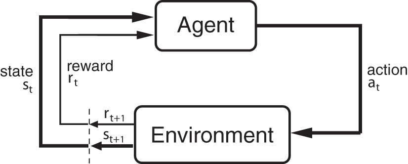
Figure 4. The feedback loop in reinforcement learning (RL).

We specifically treat the Fair Game framework (elaborated in Section 3) as performing RL in stochastic games. On a positive note, success of many practical RL systems emerges in multi-agent settings, including playing games such as chess and Go (Silver et al., 2016; 2017), robotic manipulation with multiple connected arms (Gu et al., 2017), autonomous vehicle control in dynamic traffic and automated production facilities (Yang et al., 2020; Eriksson et al., 2022a; 2022b). Further advances in these problems critically depend on developing stable and agent incentive-compatible learning dynamics in multi-agent environment. Unfortunately, the mathematical framework upon which classical RL depends on is inadequate for multiagent learning, since it assumes an agent’s environment is stationary and does not contain any adaptive agents. Classically, in multi-agent RL, these systems are treated as a stochastic game with a shared utility (Brown, 1951; Shapley, 1953). As an adaptive agent in this game only observes the outcomes of other’s actions, the sequential and partial feedback emerges naturally. This connection has led to a growing line of works to understand limits of designing provably optimal RL algorithms for stochastic games (Giannou et al., 2022; Liu et al., 2022; Daskalakis et al., 2023). The existing analysis is often RL algorithm specific, i.e. they assume all the agents have agreed to play the same algorithm (Giannou et al., 2022). On the other hand, the lower bounds quantifying the statistical complexity of these problems are mostly available for either zero-sum games (Zhang et al., 2020; Fiegel et al., 2023) or large number of players (called mean-field games) (Elie et al., 2020).

3. Fair Game framework: Auditing & debiasing over time

Now, we formulate the Fair Game framework that aims to resolve two issues:

1. (1) incorporating the auditor feedback in the debiasing algorithm of an ML model,

2. (2) adapting to dynamics of society and ethical norm, and iteratively resolving the impacts of deploying ML models over time.

First, we provide a high-level overview of the framework and its components. Then, we further formulate the framework and the corresponding problem statement rigorously.

Fair Game: An overview

In Figure 5, we illustrate the pipeline for an auditing to alignment feedback mechanism for any AI algorithm. First, an input dataset (Component (1)) is used to train an AI algorithm (Component (2)). This AI algorithm exhibits different alignment norms, also called model properties (Component (3)), such as privacy leakage, bias and instability (lack of robustness). An auditor (Component (4)) aims to accurately estimate the desired property (or properties) with minimal samples from a data pool, which might or might not match the input dataset depending on the degree of access available to the auditor. Then, the deployed auditor sends this feedback to the AI algorithm under audit, which is hardly used to incrementally debias the algorithm at present. Finally, we deploy another alignment algorithm (Component (5)) that leverages the feedback and other side information (e.g. preferences over outcomes), if available, to efficiently socially align the properties of the AI algorithm under audit.

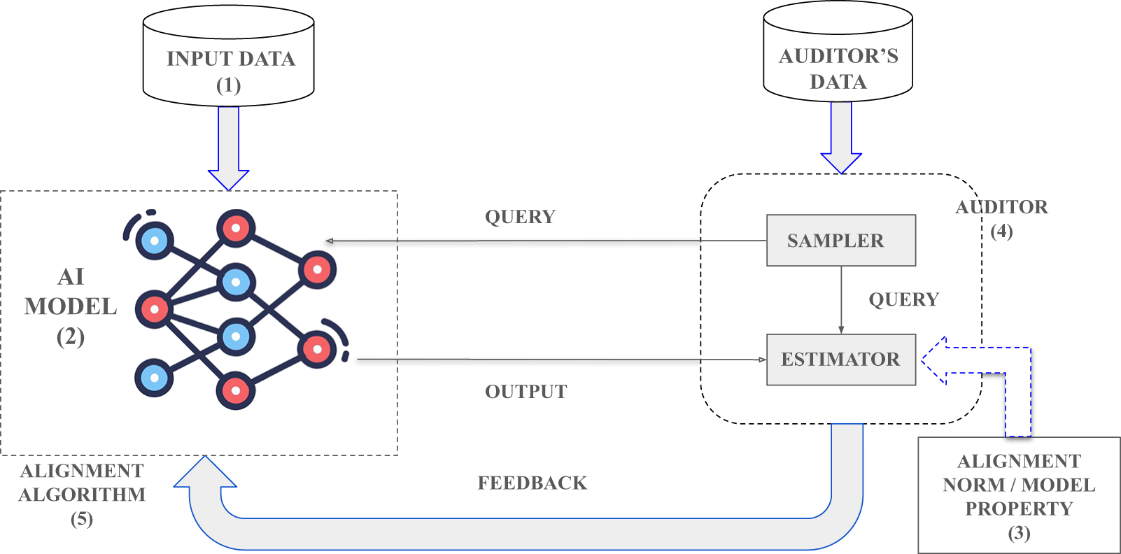
Figure 5. Components of an auditing to alignment mechanism for an AI algorithms.

In present literature, all of these components are assumed to be static over time. But as an application acquires new data over time, updates its model, and socially acceptable ethical norms and regulations also evolve, it motivates the conceptualisation of dynamic auditors. This also allows to bring in novel alignment properties from ethics and social sciences if they are computable or estimatable from observable data or their causal relations. This flexibility is essential as we still see plethora of robustness and bias metrics to emerge after a decade of studying them, and this is a natural phenomenon as ethics evolve over time and we cannot know beforehand all the impacts of a young and blossoming technology like AI.

Fair Game: Mathematical formulation

Let us consider the setting similar to Section 2.2, i.e. we have a binary classification model trained on a dataset $\mathbf{D}^T \triangleq \{(\mathbf{x}_i, \mathbf{a}_i, y_i)\}_{i=1}^m$, i.e. triplets of non-sensitive features, sensitive features and outputs generated from an underlying distribution $\mathcal{D}$. A model trained by minimising the average loss is denoted by $f_{\theta^*}$. Given a measure of bias µ, $f_{\theta^*}$ exhibits a bias $\mu(f_{\theta^*}, \mathcal{D}) \geq 0$.

Now, let us consider that the underlying distribution changes with time $t \in \{1,2,\ldots\}$. Thus, we denote the data distribution, the training dataset, the model and the property at time t as $\mathcal{D}_t$, $\mathbf{D}^T_t$, $f_{\theta^*,t}$ and µ_t, respectively. This structure defines the first three components in the Fair Game framework (Figure 5).

Under this dynamic setting, we first define an anytime-accurate PAC auditor of bias (Component (4)). The intuition is that an anytime-accurate PAC auditor of bias can achieve below ϵ error to estimate the desired bias measure as it evolves over time.

Definition 6. (Anytime-accurate PAC auditor)

An auditor $\mathcal{A}$ is an anytime-accurate PAC auditor if for any $\epsilon, \delta \in (0,1)$, there exists a function $m(\epsilon, \delta)$ such that $\forall m \geq m(\epsilon, \delta)$ samples drawn from $\mathcal{D}$, it outputs a mean estimate $\hat{\mu}_{m,t}$ at anytime t satisfying

(3)\begin{align} \mathop{\mathbb{P}}\nolimits( \forall t\in \{1,2,\ldots\}, |\hat{\mu}_{m,t} - \mu_t| \leq \epsilon) \geq 1- \delta\,. \end{align}

Here, the probability is taken over all the stochastic dynamics of the data, the model and the auditing algorithm, if it uses randomised components.

Definition 6 means that with probability $1-\delta$, an anytime-accurate PAC auditor yields an ϵ-accurate estimate of the property µ_t exhibited by the model at time t.

Now, we define the dynamic debiasing algorithm, which is the final component (Component (5)) required in Fair Game.

Definition 7. (Dynamic debiasing algorithm)

Given access to the data distribution, the training dataset, the model and an estimate of the property at time t, i.e. $\mathcal{D}_t$, $\mathbf{D}^T_t$, $f_{\theta^*,t}$ and $\hat{\mu}_t$, a dynamic debiasing algorithm $\mathcal{M}$ minimises the average bias over a given horizon $T \geq 1$, i.e.

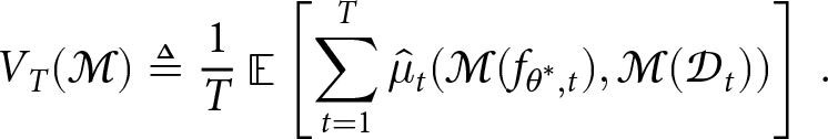(4)\begin{align} V_T(\mathcal{M}) \triangleq \frac{1}{T} \mathop{\mathbb{E}}\nolimits\left[\sum_{t=1}^T \hat{\mu}_t(\mathcal{M}(f_{\theta^*,t}), \mathcal{M}(\mathcal{D}_t)) \right]\,. \end{align}

Here, the expectation is taken over all the stochastic dynamics of the data, the model, the bias estimate and the debiasing algorithm, if it uses randomised components.

As the average bias $V_T(\mathcal{M})$ of the dynamic debiasing algorithm tends to zero with increase in T, it implies that it is able to remove over time the bias in model predictions under the dynamic setup. In general, lower is the $V_T(\mathcal{M})$ better is the dynamic debiasing algorithm. From RL perspective, $V_T(\mathcal{M})$ is the value function measuring badness of the debiasing algorithm over time T, and the bias exhibited by it at time t, i.e. $\hat{\mu}_t(\mathcal{M}(f_{\theta^*,t}), \mathcal{M}(\mathcal{D}_t))$, is its cost function per-step.

Finally, with all these components, now we can formally define the Fair Game and its quantitative goals.

Definition 8. (Fair Game)

Given access to the data distribution, the training dataset, the model and the property at any time t, i.e. $\mathcal{D}_t$, $\mathbf{D}^T_t$, $f_{\theta^*,t}$ and µ_t, the auditor-debiasing pair $(\mathcal{A},\mathcal{M})$ plays a Fair Game by yielding anytime-accurate PAC estimates of the bias, i.e. $\{\hat{\mu,t}\}_{t=1}^T$, and minimising the average bias over time, i.e. $V_T(\mathcal{M})$, respectively.

We further define the regret of the Fair Game with an auditor-debiasing pair $(\mathcal{A},\mathcal{M})$ as

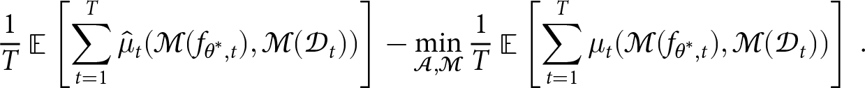(5)\begin{align} \frac{1}{T} \mathop{\mathbb{E}}\left[\sum_{t=1}^T \hat{\mu}_t(\mathcal{M}(f_{\theta^*,t}), \mathcal{M}(\mathcal{D}_t)) \right]-\min_{\mathcal{A},\mathcal{M}} \frac{1}{T} \mathop{\mathbb{E}}\nolimits\left[\sum_{t=1}^T {\mu}_t(\mathcal{M}(f_{\theta^*,t}), \mathcal{M}(\mathcal{D}_t)) \right] \,. \end{align}

Regret of the Fair Game is the difference between the minimum bias achievable over time by any auditing and debiasing algorithm-pair and that achieved by a deployed system in practice for a given stream of datasets. We observe that lower regret of the Fair Game indicates higher efficiency of the auditor-debiasing pair $(\mathcal{A},\mathcal{M})$. Thus, given a dynamic dataset, an adaptive training algorithm and the evolving measures of bias, the goal of a Fair Game is to minimise its regret, while deploying anytime-accurate PAC auditors of bias and dynamic debiasing algorithms as two players with interactions.

4. Challenges and opportunities to address the Fair Game

Now, we summarise the four desired properties of the Fair Game framework to audit and debias ML algorithms over time.

4.1. Data frugality and accuracy

The first pillar of the Fair Game is an anytime-accurate PAC auditor, but the auditor needs to query each of the updated models to conduct the estimation procedure. For external auditors and researchers designing algorithms, the data and access to proprietary ML models become the main bottleneck. Caton and Haas (2024) mention this dilemma as

“This is a hard problem to solve: Companies cannot simply hand out data to researchers, and researchers cannot fix this problem on their own. There is a tension here between advancing the fairness state-of-the-art, privacy, and policy.”

Thus, auditing over time brings us to the other pole of the AI world, where millions of datapoints are not available at all and we have to sharpen our statistical techniques to collect only informative data leading to accurate estimates. This leads to the first challenge in the Fair Game.

Challenge 1. Designing auditors that can use as minimum number of samples to yield as accurate estimate of bias as possible over dynamic data distributions and models.

Most sequential estimation and large-scale RL algorithms are known to be “data-greedy,” which is the natural framework for auditing over time. This poses an opportunity to revisit the limits of statistical RL theory in the context of auditing over time as sample frugality becomes imperative.

4.2. Manipulation proof

Manipulation proof is an interesting and unique requirement of an auditor. Specially, an auditing mechanism is a top-down phenomenon in present AI technology scenario where ML models are changing in every economic quarter yielding more profit while we know little about their impacts in socioeconomic, cultural and personal lives. Manipulation proof auditing is specifically important due to two reasons.

1. (1) Robustness to adversarial feedback. To avoid being exposed or fined under auditing and the regulation hammer, a company can provide selected samples to the auditor which make them look fairer. This provides a partial view of the prediction distribution while not being too far from the true one (Yan and Zhang, 2022; Godinot et al., 2024).

2. (2) Opportunity to evolve. On the other hand, in the reckoning market of AI, a company might argue that they have to update their models “fast” to stay competitive. Thus, it is fair to give them an opportunity to change their models between two audits (Ajarra et al., 2025). This provides another motivation to design manipulation-proof auditors that can lead to easy acceptance of auditors in practice.

At this vantage point, we define PAC auditing with manipulation-proof certification that encompasses both the motivations.

Definition 9. (PAC auditing with manipulation-proof certification)

For all $\epsilon, \delta \in (0,1)$, there exist a function $m: (0,1) \to \mathbb{N}$, such that for any probability measure $\mathcal{D} \in \mathcal{P}$, if S is a sample of size $m \geq m(\epsilon, \delta)$ sampled from $\mathcal{D}$, a PAC auditor with manipulation-proof certification yields

• • A correct estimate $\hat{\mu}_{m}$:

  \begin{align*} {\mathop{\mathbb{P}}\nolimits} \left[ \sup_{h \in \mathcal{H}_{\epsilon}(f_\theta^*)} |\hat{\mu}_{m}(h) - {\mu}(h,\mathcal{D})| \geq \epsilon \right] \leq \delta. \end{align*}

• • A manipulation-proof region $\mathcal{H}_{\epsilon}(f_\theta^*)$:

  \begin{align*} \mathop{\mathbb{P}}\nolimits \left[ \inf_{h \in {\mathcal{H}_{\epsilon}^C (f_\theta^*)}} |\hat{\mu}_{m}(h) - {\mu}(h,\mathcal{D})| \leq \epsilon \right] \leq \delta. \end{align*}

$\mathcal{H}_{\epsilon} (f_\theta^*)$ is a set of models with predictive distributions close to that of $f_\theta^*$, and $\mathcal{H}_{\epsilon}^C (f_\theta^*)$ is its complement.

The manipulation-proof region $\mathcal{H}_{\epsilon} (f_\theta^*)$ allows the company under audit to change their models in regulated region around the present model. Manipulation-proofness aims to ensure whether the AI model owner behaves adversarially and provides biased or obfuscated samples or asks for flexibility to update the model in-between two audits, the auditor should be able to estimate the bias robustly. An obfuscation of the samples or biasing them can be seen as a shift in the prediction distribution of the AI model under audit. Definition 9 claims that if we are sampling from any prediction distribution inside the manipulation-proof region $\mathcal{H}_{\epsilon}^C (f_\theta^*)$ around the true distribution under audit, the auditor can still yield good estimates of bias with high probability. In simple terms, the auditor is manipulation-proof in a regulated region around the true prediction distribution.

For the auditor, it provides an additional constraint, i.e. a region in which its bias estimate would vary minimally due to changes in predictions and input data. This goal is often in tension with accurate PAC estimation leading to a tension that we classically observe while designing any accurate by robust estimators (Huber, 1981).

This also makes PAC auditing with manipulation-proof certification a harder problem than PAC auditing. Yan and Zhang (2022) show an active learning-based procedure to achieve manipulation-proof auditing, while Godinot et al. (2024) show that manipulation-proof auditing can be harder as ML models gets larger and non-linear for a complex dataset. Ajarra et al. 2025 further show that if we use Fourier expansions of prediction distributions for auditing, we by default achieve manipulation-proofness with respect to changes in the smallest one-fourth coefficients. However, obtaining a universal complexity measure to quantify hardness of manipulation-proof auditing and comparing it with hardness of classical auditing still remains an open problem. At this point, auditing dynamic algorithms bring a stronger challenge.

Challenge 2. Designing manipulation-proof PAC auditors that can be accurate while computationally efficiently finds the manipulation-proof regions around evolving models over dynamic data distributions and models.

4.3. Adaptive and dynamic

In Section 3, we propose the formal framework of Fair Game. Specifically, Definition 8 formulates it rigorously as a two-player stochastic game. Thus, we propose to use the RL for stochastic game (Section 2.4) as the learning paradigm to resolve the Fair Game efficiently.

Specifically, last decade has seen a rise in responsible RL that aims to rigorously define and ensure privacy, unbiasedness and robustness along with utility over time. Bias in RL is studied as socio-political and economic policies (whether affirmative or punitive) interact with our society like the policies in RL do (e.g. AIRecruiter, college admissions over years, etc.). Thus, ensuring fairness in RL posits additional interesting and real-life problems (Kleine Buening et al., 2022). Researchers have studied effects of different fairness metrics on RL’s performance and designed efficient algorithms to tackle them (Gajane et al., 2022), but the RL for two-player stochastic games still remains an open problem outside the worst-case and structure-oblivious scenarios. This brings us to the third challenge.

Challenge 3. Designing RL algorithms for two-player games with auditor-debiasing algorithm pairs deployed around evolving models over dynamic data distributions and models.

An opportunity arises from the growing study of RL and sequential estimation under constraints. Specifically, we note that minimising bias over time with auditor feedback of bias is a special case of RL under constraints (Manerikar et al., 2023). Carlsson et al. (2024) and Das and Basu (2024) have derived lower bounds on performance that show how the optimal performance of an RL algorithm depends on the geometry of these constraints. Das and Basu (2024) have reinforced the estimators constraint violations to achieve optimal performance, but these algorithms are still limited to the case of structure-oblivious and linear bandits. It is a scientific opportunity and challenge to extend them further to the Fair Game.

4.4. Structured and preferential feedback

With the growing real-life application of AI, it has become imperative to ensure their behaviour aligned with social norms and users’ expectations. Especially, incorporating human preferential feedback in learning (or fine-tuning) process plays a vital role in aligning outputs from an LLM socially (Dai et al., 2023; Conitzer et al., 2024; Tao et al., 2024; Xiao et al., 2024). Reinforcement learning with human feedback (RLHF) enhances this alignment by using human judgments to fine-tune models, guiding them towards preferred actions and responses resulting in better model-adaptivity (Christiano et al., 2017; Ouyang et al., 2022; Song et al., 2024; Zhang et al., 2024), but RLHF can lead to over-optimisation for specific preferences, causing models to be overly specialised or biased, which repels adaptivity to diverse, unseen preferences in real-world applications (Christiano et al., 2017; Ziegler et al., 2019). In this context, Shukla and Basu (2024) propose the first preference-dependent lower bounds for bandits with multiple objectives and incomplete preferences. Even in this simpler setting, we observe that the preferences distort decision space. But we understand very little how the incomplete preferences and high-dimensional features on continuous state-action spaces distort the decision space, which are closer to the LLMs. Thus, the fourth challenge comes as follows.

Challenge 4. Designing debiasing algorithms that can optimally incorporate preferential and qualitative feedback of auditors to better debias the ML models over time.

4.5. Final destination: Existence of equilibrium?

The final question in any game is the existence of an equilibrium. We observe that bias measures can be PAC audited sample-efficiently with a universal auditor (Ajarra et al., 2025), while one can consider debiasing as a constraint optimisation problem of minimising loss while keeping the bias upper bounded. Thus, in presence of an auditor’s feedback that accurately quantifies the bias and instability of a dynamic algorithm at any point of time, we can treat minimisation of bias and instability in a dynamic AI algorithm under constraints on the prediction distribution. This strategy has been studied in offline setting as ERM with distributional constraints. In addition, we know that the constraint violations can be used in feedback with a dynamic learning algorithm to achieve the desired safety and unbiasedness over time (Flet-Berliac and Basu, 2022). The generic framework to address them is to simulate a constraint-breaking adversary and a learner trying to avoid the adversary by only looking into its feedback. They use the same data stream to conduct their learning procedures. This poses the final two challenges.

Challenge 5. Can we achieve a stable equilibrium for the Fair Game when the measure of bias is fixed over time?

Challenge 6. Can we achieve a stable equilibrium for the Fair Game when the measure of bias is evolving over time?

We conjecture that the answer to the first challenge is affirmative while that of the second one depends on the changes in bias measures. Our intuition is based on the fact that bias measures are often conflicting and thus cannot be achieved simultaneously in a single game. One avenue to address these problems will be to extend the growing literature on stochastic non-zero-sum games (Sorin, 1986; Zhang et al., 2020; Bai et al., 2022; Fiegel et al., 2023) with learners to the Fair Game setting, where utility of the auditor is to measure the constraint violation and that of the learner is to minimise loss in training while incorporating the auditor’s feedback.

5. Bridging Fair Game and legal perspectives of audits

As Fair Game aims to bind the auditor and model owner into a single framework, it is a natural requirement to develop a legal framework for this and wonder how the present legal frameworks for auditing do or do not satisfy the requirements.

The landscape of law and algorithmic audits

Le Merrer et al. 2023 provide an overview of the existing legal intricacies around algorithmic audits. We extend their insights to formalise the desired legal bindings for Fair Game.

The first legal concern for algorithmic auditing is data protection laws, such as the GDPR (Voigt and Von dem Bussche, 2017) in Europe. These laws safeguard user privacy and restrict data access to the algorithmic auditors (Directive 96/9/EC of the European Parliament and of the Council of 11 March 1996 on the Legal Protection of Databases 2019). In this context, Le Merrer et al. 2023 distinguish between two types of audits: Bobby Audits, which use real user data and thus face stronger legal scrutiny, and Sherlock Audits, which rely on synthetic data and are less legally restrictive but may have weaker evidential value. Fair Game naturally inherits these challenges of static auditing evoked by data protection laws. In this context, the rich literature of estimation and learning under privacy would play an instrumental role to develop efficient technical solutions (Chaudhuri et al., 2011; Dwork and Roth, 2014; Dandekar et al., 2018; Wang et al., 2020).

Another challenge in algorithmic auditing is due to intellectual property rights and trade secrets. Many companies argue that their algorithms are proprietary and, in turn, constraint the auditors access of information to examine them. The present law currently does not provide a unequivocal “right to audit.” Thus, auditors often have to rely on indirect methods, such as scrapping the data from web services and digital platforms, or risk potential legal consequences, if they test proprietary algorithms without explicit permission. This propels the development of black-box auditors for estimating bias of AI models and is an active area of research (Ghosh et al., 2023b; Ajarra et al., 2025). This nuance is naturally covered by the Fair Game framework as it is applicable to both internal and external auditors with white-box and black-box access, respectively.

Liability is another challenge.¹⁴ If auditors publicly disclose biases or discriminatory practices within an algorithm, they may face legal threats from companies seeking to protect their reputation and avoid regulatory penalties (Le Merrer et al., 2023). Additionally, how can we ensure that the companies would provide the auditors unbiased access to samples or update their models inside the prescribed manipulation-proof regions. Right now there is no reward or restriction on companies to not play adversarial during an audit. Thus, a legal binding of trust and liabilities between companies and auditors to create one single ecosystem is presently missing. Such developments have been seen for some other technologies, such as ISO¹⁵ and IEEE¹⁶ standards and certifications, and we need to develop one for emerging AI technologies. A unifying legal framework would be imperative to turn Fair Game into an effective paradigm for trustworthy deployment of AI.

The legal environment for algorithmic auditing is still evolving. While current laws protect companies and user privacy, they must also facilitate responsible and ethical auditing. We now discuss about NYC Bias Audit Law, which is one of the real-life instance in this direction.

A bias auditing law in real-life: NYC Bias Audit Law

As a real-life example of law enforcing algorithmic audits, we discuss the NYC Bias Audit Law or the Local Law 144 that has been mandated for algorithmic auditing of AI driven employment tools called “AEDT” (Automated Employment Decision Tool).¹⁷ This is one of the first regulation enforced in the United States (specifically, New York City) that proposed auditing of digital platforms. Enacted in 2021 and enforced as of July 5, 2023, Local Law 144 is a significant step towards fairness and transparency in automated decision-making, particularly targeting employment and promotion processes.

Key components. 1. Annual independent audits of bias. Potential employers or organisations must conduct an independent bias audit of their AEDTs at least once per year. The audit evaluates bias in predictions across the protected demographics, specifically race, ethnicity and gender. The fairness metric used in auditing AEDTs is the ratio

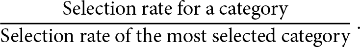\begin{align*} \frac{\text{Selection rate for a category}}{\text{Selection rate of the most selected category}}\,. \end{align*}

This is a case-specific estimate of demographic parity (Definition 2) studied in fair ML literature. As the ratio goes to one, the AEDT is considered to be more fair.

2. Candidate and employee notification. Any employer must notify job applicants and employees at least 10 business days before using an AEDT in decision-making. It must include information about the tool’s functionality and the applicant’s right to request alternative evaluation methods. This aims to ensure transparency and privacy-compliant data processing in the AEDT tool.

3. Public disclosure of audit results. Any user of AEDTs must publicly post the results of their annual bias audits in their website demonstrating the system’s fairness and impact on different protected demographics. This ensures the liability of AEDTs as a socially impactful technology as discussed before.

4. Penalties for non-compliance. Organisations failing to comply with these requirements face financial penalties, starting at 500 dollars for the first violation and increasing for subsequent infractions. This component aims to reinforce compliance of the user to the law and ensure unbiasedness in employment.

A failed attempt or a case for unified dynamic auditing? Despite of being a pioneering attempt towards bridging theoretical auditing and practical enforcement as a legal obligation for employers, the Local Law 144 has had many shortcomings.

1. (1) Simplistic auditing process. It is too optimistic that the auditor can use the final output and compute one of the many group fairness metrics to measure bias in order to create a comprehensive bias report. It does not promote for any causation of the bias and also no preference-based or case-to-case evaluation. It is very hard to develop any legal case with such simplistic audit. Fair Game brings in a richer framework to mitigate these issues.

2. (2) Static auditing. The auditing approach, specially the fairness metric suggested by the law, is not adaptive with time. It could neither leverage historical information in the auditing process nor can keep up with the changing notions of fairness. This is problematic as we cannot understand whether an AEDT tool is systematically biased or it is just one exceptional event. At this point, Fair Game brings in the dynamic perspective and proposes to treat the auditing and debiasing as a two player game, where both players have different incentives to play the game.

3. (3) Lack of enforcing compliance. Only one case of non-compliance was officially reported in six months after commencement though the authority was aware of hundreds of such cases. Also, there was no demand for third party auditor services, like proceptual.com (Janaro, 2023; Wright et al., 2024). The reasons are twofold. First, bureaucracy and lobbying delayed the enforcement of the law. Even after imposing it, NY city council loosened the laws and requirements and left several loops in the compliance rules within 24 hours of commencement. There is no purely technical solution to this. Second, the present law neither provides any reward or pressing reason for the AI model owner to comply with the auditing law nor it gives any flexibility and guideline to update the AI models between two audits. Fair Game proposes the dynamic and adaptive framework to overcome these issues.

6. Discussions and perspectives

With the growing use of AI algorithms for bouquets of real-life tasks such as autonomous recruitment, crime recidivism, autonomous college admission, etc., the need for debiasing these algorithms from any bias and aligning them with social norms has become crucial. Throughout this article, we have explained different sources of biases with real-life examples like AEDTs as well as the different approaches taken to mitigate them. We propose a dynamic mechanism “Fair Game” that assures to preserve fairness in prediction of ML algorithms that also adapt to changes as the society interacts with the algorithm over time. The “Fair Game” conjoins an Auditor and a Debiasing Algorithm in a loop leveraging the concepts of RL. Our approach addresses the lacunae of the existing approaches to debias an ML algorithm as they usually work well for static environments. “Fair Game” takes the process of debiasing to a dynamic environment that makes the process adaptive over time. We have also emphasised on some desirable properties of an auditor such as accuracy, data frugality, constant manipulation proofness, etc. Thus, “Fair Game” envisions an interactive approach to design statistically and computationally efficient continual auditors of AI algorithms and incorporate auditor’s feedback in-a-loop to dynamically align these algorithms. This approach is novel, descriptive and more regulation-friendly and allows continual evaluation and alignment of AI algorithms.

Collaborative human and algorithmic auditing

Finally, we would like to emphasise that the Fair Game does not aim to replace but aid the human AI auditors. This is necessary in order to connect the algorithmic audits with the available legal frameworks. Specifically, Fair Game enables the human auditors in two ways.

(i) For companies dealing with large number of user data, for example AIRecruiter, an auditor will have to manage and analyse a big and dynamic database. In these scenarios, a human-driven model becomes challenging in terms of resources and capacity. The AI auditor rather can provide statistically sound summaries of bias and other risks due to deployment of the AI algorithm that the human auditors and lawyers can use for further inspection.

(ii) In Fair Game, if an auditor is given a task to align an AI algorithm as per the requirements in Digital Marketing Act(DMA) or Digital Service Act (DSA) (for example, services provided by babl.ai), it demands intrinsic knowledge of the specific domain of application. This is where algorithmic auditors can enable us significantly by saving resources and creating a knowledge map that can be adapted over time.

But algorithms do not understand ethics till we design and tune them to it. In recent days, we have witnessed numerous proposals and research articles that advocate human intervention in aligning LLMs with social values in their decision-making whether by prompt engineering or leveraging RLHF (Wang et al., 2023; Ji et al., 2024; Shankar et al., 2024; Song et al., 2024). Thus, we envision the use of structural and preferential feedback (Section 4.4) in Fair Game, which allows human auditors to intervene with case studies and preference over certain outcomes, and then the algorithmic auditor and the alignment algorithm further adapt to it.