The influence of correlated features on neural network attribution methods in geoscience

Abstract

Artificial neural networks are increasingly used for geophysical modeling to extract complex nonlinear patterns from geospatial data. However, it is difficult to understand how networks make predictions, limiting trust in the model, debugging capacity, and physical insights. EXplainable Artificial Intelligence (XAI) techniques expose how models make predictions, but XAI results may be influenced by correlated features. Geospatial data typically exhibit substantial autocorrelation. With correlated input features, learning methods can produce many networks that achieve very similar performance (e.g., arising from different initializations). Since the networks capture different relationships, their attributions can vary. Correlated features may also cause inaccurate attributions because XAI methods typically evaluate isolated features, whereas networks learn multifeature patterns. Few studies have quantitatively analyzed the influence of correlated features on XAI attributions. We use a benchmark framework of synthetic data with increasingly strong correlation, for which the ground truth attribution is known. For each dataset, we train multiple networks and compare XAI-derived attributions to the ground truth. We show that correlation may dramatically increase the variance of the derived attributions, and investigate the cause of the high variance: is it because different trained networks learn highly different functions or because XAI methods become less faithful in the presence of correlation? Finally, we show XAI applied to superpixels, instead of single grid cells, substantially decreases attribution variance. Our study is the first to quantify the effects of strong correlation on XAI, to investigate the reasons that underlie these effects, and to offer a promising way to address them.

Impact Statement

Substantial effort has been made in eXplainable Artificial Intelligence (XAI) methods to investigate the internal workings of machine/deep learning models. We investigate the impact of correlated features in geospatial data on XAI-derived attributions. We develop synthetic benchmarks that enable us to calculate the ground truth attribution. Using synthetic data with increasing correlation, we show that strong correlation may lead to increased XAI variance, which can be problematic for making robust physical inferences. Our results suggest that the increased variance stems from the fact that when there are highly correlated features, networks learn very different patterns to solve the same prediction task. Finally, we provide promising approaches for addressing the variance issue and improving attributions for better model insights.

1. Introduction

Artificial intelligence (AI) is increasingly used to develop models using complex machine learning (ML) architectures, such as deep learning (DL). Such AI models are now frequently used in geosciences for extracting nonlinear patterns from the rapidly growing volume of geospatial data. Among others, applications include predicting soil temperature (Yu et al., 2021), typhoon paths (Xu et al., 2022), sea surface temperature (SST) (Fei et al., 2022), and classification using multispectral (Helber et al., 2019) and synthetic aperture radar (Zakhvatkina et al., 2019) imagery. Other applications include multiyear forecasting of El Niño/Southern Oscillation events (Ham et al., 2019) and improving sub-grid representations in climate simulations (Rasp et al., 2018). These AI models have been described as black boxes since their complexity obfuscates how they work (McGovern et al., 2019). They learn a function based on associations between inputs and targets, but it is hard to decipher how the data influence the model output.

The lack of transparency in complex ML models has motivated the rapid development of the field of eXplainable AI (XAI) aimed at enhancing the ability to understand the model’s prediction-making strategies (Murdoch et al., 2019). By exposing what a network has learned, XAI methods have the potential to reveal actionable insights (Mamalakis et al., 2020). First, XAI can be used to gauge trust in the model, that is, make sure that a good performing model performs well for the right reasons. Indeed, a model can achieve high performance on an independent test set even though it has learned spurious relationships that would cause the model to fail in operation (Lapuschkin et al., 2019). Thus, XAI is desirable for testing against these spurious relationships before model deployment. Here, interpretability is desired to learn about the model itself. Second, in the case of a poor performing model or if the network has learned problematic strategies, then XAI may provide guidance for model tuning. Third, if the model performs well and is assessed to be reliable, it may have learned novel patterns in the dataset of interest, and exposing these relationships could lead to novel hypotheses about the geophysical phenomena at hand. Here, interpretability is desired to learn about the real-world phenomena, using the model as a proxy. Thus, apart from gauging trust or model tuning, XAI can be used to extract physical insights to generate hypotheses leading to novel science discoveries. We note that using ML to identify novel scientific information is still in its infancy, but there are examples of investigating trained ML models to extract unknown patterns in geophysical phenomena. Rugenstein et al. (2025) trained convolutional neural network (CNN) models to learn relationships between top of atmosphere radiation and surface temperature patterns. They then applied XAI methods to investigate the trained models, finding novel geographical dependencies that disagree with the equations commonly used to model these phenomena. Zanna and Bolton (2020) developed an interpretable, physics-aware ML model to derive ocean climate model parameterizations. Using model interpretability methods, the authors were able to leverage ML for equation discovery. Mayer and Barnes (2021) used ML to discover novel forecasts of opportunity — atmospheric conditions that enable more skillful forecasting. An XAI method was applied to a trained network to identify potential novel patterns for enhancing subseasonal prediction in the North Atlantic. Van Straaten et al. (2022) used XAI methods applied to random forest models of subseasonal high temperature forecasts for Western and Central Europe to identify potential subseasonal drivers of high temperature summers.

XAI includes a broad collection of approaches, which are summarized as follows. Attribution methods are an important type of XAI for investigating geophysical networks. These methods assign an attribution to each input feature that indicates that feature’s influence on the network prediction. This type of explanation has been referred to as feature effect (Molnar et al., 2020) or feature relevance (Flora et al., 2024), in contrast to feature importance methods that rank features based on their contribution to global model performance. Flora et al. (2024) provide a detailed reference for XAI concepts and these explainability terms (e.g., feature relevance vs. feature importance) in the context of atmospheric science, but it is broadly applicable to geoscience applications. In the case of gridded spatial data, the explanation is often a heatmap that highlights the influential spatial regions. Attribution methods have been used to investigate models for composite reflectivity (Hilburn et al., 2021), land use classification (Temenos et al., 2023), and detecting climate signals (Labe and Barnes, 2021). Attribution maps are a type of local, post hoc explanation. Post hoc XAI techniques are those that are applied in a post-prediction setting to black-box models to expose their learned characteristics. This is in contrast to interpretable models that are designed to have some degree of inherent interpretability, typically at the cost of model performance. XAI techniques produce either global or local explanations. A global explanation is a summary of a set of samples, whereas a local explanation applies to a single input and the corresponding prediction. Local explanations offer fine-grained detail about specific model predictions, for example, which parts of an input satellite image the model was using to predict tornado development. Attribution methods have potential for revealing detailed insights into model predictions, which can aid model users and developers.

Despite its promise, XAI is still a developing research area and the methods have been shown to be imperfect (Adebayo et al., 2018; McGovern et al., 2019). First, there are many attribution methods and they may give very different explanations (high inter-method variability). It is difficult to determine which, if any, provide an accurate description of the network’s actual prediction-making process. Also, XAI methods especially struggle when the input data exhibit a highly correlated structure (Hooker et al., 2021). This means that XAI can be especially challenging to apply to geosphysical models that commonly rely on high-dimensional gridded spatial data inputs. For simpler tabular models, a common recommendation is to reduce the input features to a smaller set that exhibit less correlation. However, this does not make sense for gridded geospatial data (e.g., satellite imagery and numerical weather prediction outputs). This is because individual spatial data grid cells lack semantic meaning in isolation, and the networks rely on spatial patterns in the structured input. Removing correlated grid cells would corrupt the input raster, compromising the spatial features that we are trying to learn from. In the simplest case, spatial correlation is present across a single 2D map, but it can be across a 3D volume where multiple image channels represent altitudes, time steps, or both. Indeed, a fundamental characteristic of spatial data, as described by Tobler’s first law, inherently makes XAI techniques harder to use: “everything is related to everything else, but near things are more related than distant things” (Tobler, 1970). Additional correlations may exist in the data, such as long-range teleconnections between climate variables (Diaz et al., 2001). Krell et al. (2023) provided an example of how correlation can impact XAI results. Applying several XAI methods to explain FogNet, a 3D CNN for coastal fog prediction (Krell et al., 2023), Krell et al. showed that explanations were highly sensitive to how correlated features were grouped before applying XAI. Based on the scale at which features were investigated, explanations could yield completely opposite descriptions of model behavior. This is greatly problematic as it makes XAI potentially misleading for practitioners, leading to incorrect interpretations of the model, which could be worse than treating the model as a black box.

Broadly, there are two main ways in which correlated features may influence XAI results and compromise its utility. First, correlated features can negatively affect the XAI’s faithfulness to the network, that is, make it difficult for the XAI to accurately identify the relevant features that the network used to predict (Hooker et al., 2021). Second, correlated features can increase the chances for a network to learn many, possibly infinite, different combinations of the features to achieve approximately the same performance. In other words, a high correlation in the input increases the number of available solutions for the given prediction task and the given training size, thus, increasing the inherent variance of possible explanations. In the first case, inaccurate attribution maps make it difficult to use XAI for understanding about either the trained network or the real-world phenomena. In the second case, an explanation that accurately captures the network could be difficult to interpret: features that are meaningful for the real-world phenomena may be assigned minimal attribution because the network has learned to exploit another feature that is correlated with the true driver. In practice, both of the above issues (low XAI faithfulness and high variance of possible solutions) may occur simultaneously, which further complicates the use of XAI: the networks may have learned spurious correlations, and the XAI methods may, at the same time, struggle to accurately reveal the learned patterns.

We note that the issue of inherent increased variance in the solutions highlighted above is related to the statistical concept of the Rashōmon set: a set of models that achieve near-identical performance, but using different relationships between the input and output (Xin et al., 2022). With stronger correlations present in the input domain, we expect greater variance in the learned relationships within the Rashōmon set. Flora et al. (2024) discuss feature importance results for members of the Rashōmon set, with guidance on determining if a feature is important for all members or just a single model (and the concept applies to attribution methods as well). They conclude that an explanation that is only valid for an individual Rashōmon member can be useful for debugging that member, but might be misleading for understanding the real-world phenomena if other members can offer alternative explanations.

The purpose of this research is to quantitatively investigate the influence of correlated features on geophysical models that use gridded geospatial input data. Because of the lack of ground truth attributions, quantitative analysis of XAI is very challenging. Various metrics have been proposed for evaluating attributions such as Faithfulness Correlation (Bhatt et al., 2020), but these metrics do not involve the direct comparison of an attribution map to a ground truth. Mamalakis et al. (2022b) proposed an alternative approach to XAI evaluation by developing a synthetic benchmark where the ground truth attribution can be derived from a synthetic function. An XAI benchmark is created by designing a function $ \mathcal{F} $ and training an approximation of $ \mathcal{F} $ called $ \hat{\mathcal{F}} $ . $ \hat{\mathcal{F}} $ represents the trained network. This is done by computing the output of $ \mathcal{F} $ for a large number of inputs, and using the result as a target to train a network $ \hat{\mathcal{F}} $ . If the trained network achieves extremely high accuracy, then it is assumed to adequately approximate $ \mathcal{F} $ ; that is, $ \mathcal{F} $ and $ \hat{\mathcal{F}} $ are assumed to represent approximately the same relationship between the inputs and the targets. Then, since we know the ground truth of the attribution of an output of $ \mathcal{F} $ to each input feature, we can test an XAI applied to explain $ \hat{\mathcal{F}} $ on whether it identifies similar relevant patterns to the ground truth. Critically, we must be able to theoretically derive the ground truth attribution based on the functional form of $ \mathcal{F} $ . A key contribution by Mamalakis et al. (2022b) is the methodology of designing additive functions with arbitrary complexity that satisfies this property. The result is that XAI algorithms can be quantitatively assessed based on the difference between their explanation and the ground truth attribution.

The critical assumption by Mamalakis et al. (2022b), that the trained network $ \hat{\mathcal{F}} $ so closely approximates $ \mathcal{F} $ , is needed for one to use the attribution of $ \mathcal{F} $ as a meaningful proxy for a ground truth attribution of $ \hat{\mathcal{F}} $ . In this research, we are building on this proposed methodology to develop a set of benchmarks to study the influence of correlated features in the input. Specifically, we are attempting to break the above assumption: with sufficiently strong correlation structure, the network should have many different options for learning relationships in the data that enable it to achieve very high performance. By creating synthetic datasets with increasingly strong correlations, we are interested in the relationship between the ground truth attributions and the XAI attribution maps generated for a set of trained networks.

We use the $ {R}^2 $ between the predictions and targets to measure the global model performance. While a high $ {R}^2 $ suggests strong overall model performance, there may be specific samples of poor performance. Nevertheless, we hypothesize that models with higher $ {R}^2 $ are a better approximation of the known function, and to investigate this further, we train models while varying the size of the input dataset to observe if this affects the overall agreement between the ground truth and XAI-based attributions. Regardless, we recognize that some misalignment between the ground truth and XAI may be due to a poor prediction for that sample, rather than due to correlation in the input domain. For this reason, we intentionally present our results as distributions (e.g., Figure 6) rather than relying solely on summary statistics. This approach allows us to capture local variations and provide a more holistic assessment of explanation fidelity. In addition, we apply XAI evaluation metrics such as Faithfulness Correlation (Bhatt et al., 2020) and Sparseness (Chalasani et al., 2020) to analyze the relationships between those metrics and the strength of the embedded correlation. This ensures that our analysis is not constrained to a single, global measure like $ {R}^2 $ .

We provide a framework to investigate the impact of correlated features on geophysical neural networks (NNs). Using the benchmarks and metrics, we demonstrate that correlation can have a substantial impact on attributions and on the trained networks. Further, our analysis suggests that we can use the variation of XAI results among a set of trained networks as a proxy to detect when attribution maps are likely being influenced by correlated features, and further, when the influence is on the learned relationships rather than the XAI faithfulness. Finally, we show that grouped attributions can be used to substantially improve the agreement between the attribution methods and ground truth.

1.1. Contributions

Our research makes the following contributions:

• • A synthetic benchmark framework to analyze how correlated features influence attributions.

• • An investigation in how correlation impacts network’s learning and hence the attributions.

• • Strategies to detect and mitigate potential issues with attributions for a given network without having to compare to a ground truth attribution.

• • Demonstration that superpixel-level XAI may offer additional insight into the network.

2. Framework for attribution benchmarks

This research builds on a framework for evaluating XAI attributions using a synthetic benchmark (Mamalakis et al., 2022b). In Section 2.1, we summarize the original framework (Mamalakis et al., 2022b) and Section 2.2 describes our framework that uses benchmarks for analysis of correlated features and XAI.

2.1. Synthetic nonlinear attribution benchmarks

The purpose of a synthetic attribution benchmark is to obtain a mapping between input vectors and output scalars where there is a ground truth attribution for any output to each vector element. The ground truth attribution for each input vector serves as a ground truth explanation for comparison with attributions generated from XAI methods. The purpose of the synthetic benchmark proposed by Mamalakis et al. (2022a) was to achieve a quantitative comparison of several XAI methods for geophysical models that use gridded geospatial data inputs. Thus, the attribution benchmark was designed to proxy real geospatial applications by enforcing nonlinear relationships between each input grid cell and the target as well as spatial dependencies between grid cells.

The first stage of benchmark creation is generating a set of synthetic samples $ \mathbf{X} $ to be used as inputs. Synthetic samples are used instead of real samples so we can generate an arbitrary number of samples. With a sufficiently large N, we expect to be able to very closely approximate the synthetic function using a NN, even for complex, nonlinear relationships. If the trained network $ \hat{\mathcal{F}} $ is not a near-perfect approximation of $ \mathcal{F} $ , then it is not fair to treat the attribution derived from $ \mathcal{F} $ as ground truth for an XAI explanation derived from $ \hat{\mathcal{F}} $ .

We generate $ N $ independent realizations of the input vector $ \mathbf{X}\in {\mathrm{\mathbb{R}}}^D $ , where $ D $ is the number of features (grid cells) in $ \mathbf{X} $ , by using a Multivariate Normal Distribution MVN(0, $ \boldsymbol{\varSigma} $ ). So that the synthetic dataset is a useful proxy for real-world geophysical problems, we use a real dataset to estimate the covariance matrix $ \boldsymbol{\varSigma} $ . The synthetic samples are supposed to represent real SST anomalies, and the covariance matrix is set equal to the observed correlation matrix estimated from the SST monthly fields (COBE-SST 2 product [Japanese Meteorological Center, 2024]). This covariance matrix encodes pairwise relationships between grid cells, thereby enforcing geospatial relationships. Without these spatial relationships, the input vectors are nonspatial data that are arbitrarily arranged in a grid.

The second stage of benchmark creation is generating the synthetic function $ \mathcal{F} $ : a nonlinear mapping of synthetic input $ \mathbf{X}\in {\mathrm{\mathbb{R}}}^D $ to nonlinear response $ Y\in \mathrm{\mathbb{R}} $ . A critical condition for an attribution benchmark is that $ \mathcal{F} $ must be designed such that we can derive the attribution of the output $ y\in Y $ to each input variable. This can be achieved by constructing $ \mathcal{F} $ as an additively separable function, where each element $ i $ of the input vector is associated with its own local function $ {\mathcal{C}}_i $ . That is, each local function $ {\mathcal{C}}_i $ only depends on the value at grid cell $ i $ , and the output of $ \mathcal{F} $ is simply the sum of all $ {\mathcal{C}}_i $ outputs. By design, the attribution map for a sample is derived by assigning each grid cell an attribution value equal to the value of that grid cell’s associated $ {\mathcal{C}}_i $ . The major drawback to this design is the lack of dependency between grid cells, since each local function depends only on that single cell. However, spatial relationships can be induced at the functional level by enforcing similar behavior in local functions among grid cell neighborhoods. The complexity of $ \mathcal{F} $ is controlled by the design of the local functions. Each local function $ {\mathcal{C}}_i $ is a piece-wise linear function with $ K $ breakpoints. With increasing $ K $ , highly complex nonlinear relationships can be achieved. Using this design (Mamalakis et al., 2022b), we can generate $ \mathcal{F} $ such that the total response $ Y $ is nonlinear and complex, but the attribution toward $ Y $ is easily derived since each local function $ {\mathcal{C}}_i $ depends on a single grid point.

The purpose of the synthetic benchmark is to analyze XAI methods that are applied to black box ML models. So, the next step of benchmark creation is training a network $ \hat{\mathcal{F}} $ that approximates $ \mathcal{F} $ so that explanations based on $ \hat{\mathcal{F}} $ can be compared to the ground truth attributions derived from $ \mathcal{F} $ . The ML architecture (Mamalakis et al., 2022b) is a fully connected NN with six hidden layers. The hidden layers contain 512, 256, 128, 64, 32, and 16 neurons, respectively, and are connected between Rectified Linear Unit (ReLU) activation functions. The final output is a single neuron using a linear activation function. The network is trained using a mean-squared error loss function.

2.2. Suite of benchmarks for correlation analysis

In this research, we use the synthetic benchmarks proposed by Mamalakis et al. (2022b) to investigate the influence of correlated features on XAI attribution methods. Figure 1 provides an overview of our proposed approach. A fundamental assumption by Mamalakis et al. (2022b) is that a very high-performing $ \hat{\mathcal{F}} $ has learned a mapping between input grid cells and output that closely approximates the actual relationship defined in synthetic function $ \mathcal{F} $ . Very high performance, $ {R}^2 $ > 0.99, is achievable since we are able to generate an arbitrarily large number of synthetic samples. Regardless, we do not expect $ \hat{\mathcal{F}} $ to be an exact replication of $ \mathcal{F} $ . Correlations between input features enable the trained network to learn multiple combinations of those features to achieve the same or similar performance. As we increase the strength of correlations among grid cells in the synthetic dataset, this becomes even more true and we expect it to have an impact on the trained networks by making many options available of equally valid functions that the network could learn.

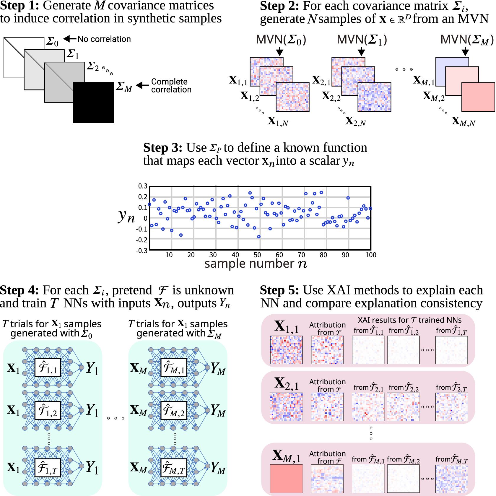
Figure 1. Methodology for creating a suite of synthetic benchmarks and using it to analyze the influence of feature correlation on NN attribution methods.

Our proposed framework shown in Figure 1 is based on developing several synthetic attribution benchmarks, where the difference between them is the overall strength of correlation among grid cells in the covariance matrix used to generate the synthetic samples. To analyze the influence this has on the trained networks and XAI results, we train multiple networks for each synthetic function. We expect that the increased correlation will have some influence on how the XAI-based attribution maps align with the attribution derived from the synthetic function. In the following, we describe each step of our proposed framework. For visual simplicity, the figure uses a toy example where the covariance matrices used to generate synthetic samples have uniform covariance. That is, the pairwise correlations between grid cells are identical across the entire map. In practice, these covariance matrices should be based on a geospatial dataset of interest, such as the SST anomaly data used by Mamalakis et al. (2022b).

In Step 1, we generate M covariance matrices $ {\boldsymbol{\varSigma}}_1 $ , $ {\boldsymbol{\varSigma}}_2 $ , …, $ {\boldsymbol{\varSigma}}_M $ , where $ {\boldsymbol{\varSigma}}_1 $ has the least overall correlation and $ {\Sigma}_{\mathrm{\mathcal{M}}} $ has the most. In the toy example shown, $ {\boldsymbol{\varSigma}}_1 $ is the no correlation case, with all off-diagonal elements being 0: the generated samples are completely random, with no spatial structure. $ {\boldsymbol{\varSigma}}_M $ is the complete correlation case, where all correlations are 1.0 so that each sample has a single uniform value across all cells.

In Step 2, we use these covariance matrices to generate $ N $ samples from an MVN distribution. Given M covariance matrices, we generate $ {\mathbf{X}}_1 $ , $ {\mathbf{X}}_2 $ , …, $ {\mathbf{X}}_M $ synthetic datasets. An individual sample for the covariance matrix $ {\boldsymbol{\varSigma}}_M $ is a vector $ {\mathbf{x}}_{m,n} $ $ \in $ $ {\mathbf{X}}_m $ for $ n=1,2,\dots, N $ . The number of samples N has a strong influence on the performance of the networks. Mamalakis et al. (2022b) used $ {10}^6 $ samples so that the trained network achieved $ {R}^2 $ > 0.99. Here, we are interested in how correlation influences XAI methods when dealing with realistic scenarios, so we run all experiments varying $ N\in \left[{10}^3,{10}^4,{10}^5,{10}^6\right] $ .

In Step 3, we create synthetic functions $ {\mathcal{F}}_i $ for $ i $ = 1, 2, … , M so that each covariance matrix is associated with a synthetic function. The function is created by randomly generating a local PWL function for each element of the input vector. In Step 4, we train networks to approximate each synthetic function $ {\mathcal{F}}_i $ . Since correlations may introduce multiple relationships for the network to learn, we train a set of networks for each synthetic function. For a synthetic function $ {\mathcal{F}}_i $ , we independently train T models $ {\hat{\mathcal{F}}}_{i,t} $ for $ t $ = 1, 2, …, T. Network inputs are the synthetic samples generated in Step 2 and the targets are the outputs of the synthetic functions.

In Step 6, we apply the XAI methods to each of the trained networks. Since various XAI methods make different assumptions regarding correlated data, we apply several methods to study the influence of correlations on their attribution maps. The methods are described in Section 3. All XAI methods produce local explanations of feature effect. For a given sample, these methods assign an attribution value to each grid cell that is intended to capture the magnitude and direction of that cell’s contribution to the final network output. If the trained network is a perfect representation of the synthetic function, then a perfect XAI method produces an attribution map identical to the attribution map derived from the synthetic function for that sample. In practice, XAI outputs differ from the derived attribution because the (1) learned network does not exactly capture the synthetic function $ \mathcal{F} $ and (2) XAI methods are imperfect, and different methods tend to disagree for the same sample. Correlated input features can influence both of these issues, and an important aspect of this analysis is that it is challenging to disentangle and isolate the effect of each of these two issues.

In our analysis, we explore the effect of correlated features on the distribution of alignment between XAI outputs and the ground truth. We also investigate the distribution of alignment between XAI outputs from different trained networks, and check if there is a relationship between the two. Since a synthetic attribution is not available in practice, we are interested in using the variance among explanations from different trained networks as a proxy to detect that the explanations are influenced by correlated inputs and are likely to vary with respect to the attribution of the real phenomena.

2.3. Method for adding correlation in the input

We modify covariance matrices to increase correlation among the input features. First, we convert the scaled covariance to an unscaled correlation matrix. Ignoring scale makes the method more general. A valid correlation matrix is positive semi-definite. The convex combination of correlation matrices remains valid. To add additional strength, we use that property and compute a weighted sum of the initial correlation matrix and a correlation matrix of all ones (complete positive correlation). Specifically, each correlation matrix $ {\boldsymbol{\varSigma}}_i $ is created by strengthening the previous matrix $ {\boldsymbol{\varSigma}}_{i-1} $ using the weighted combination $ {\boldsymbol{\varSigma}}_i=\left(\left(1-{w}_i\right)\ast {\boldsymbol{\varSigma}}_{i-1}\right)+\left({w}_i\ast {\boldsymbol{\varSigma}}_{ones}\right) $ , where $ {\boldsymbol{\varSigma}}_{ones} $ is the correlation matrix with all ones and $ {w}_i $ is refers to the $ {i}_{th} $ weight $ \in \mathrm{0.1,0.2},\dots, \mathrm{0.9} $ . We start by setting $ {\boldsymbol{\varSigma}}_{-1} $ to the correlation matrix derived from the real data. This method is simple and increases correlation while preserving the original relationships. The drawback is that negative correlations are actually reduced in strength with the addition of positive values. So, we check that the absolute value of the correlation increases to ensure that our overall strength increases even if some relationships weaken.

3. Attribution methods

We analyze attributions produced by three XAI methods. The selected XAI methods include two of the eight used in the original paper by Mamalakis et al. (2022b), in addition to SHAP.

It is important to point out that this analysis is limited to using post hoc XAI to study feature attribution. Researchers have proposed investigating trained models for other tasks, such as counterfactual analysis. Bilodeau et al. (2024) introduced the Impossibility Theorem. In essence, this theorem claims that local attribution methods cannot extrapolate beyond the local sample that they are applied to. Their research demonstrates that complete and locally linear XAI methods (e.g., SHAP, Input × Gradient) may be unreliable for tasks like counterfactual analysis — potentially performing worse than random guessing or simpler methods (e.g., gradient-based approaches). However, the synthetic dataset and ground truth benchmark used in our study are designed to evaluate attribution in the presence of correlated features and not to assess counterfactual insights. Additionally, the methods we employ that are described below (Gradient, SHAP, and Integrated Gradients) have already been validated for attribution in Mamalakis et al.’s (2022b) paper, making them appropriate tools for addressing our core research question regarding the impact of correlation on XAI attributions.

3.1. Gradient

The Gradient is computed by calculating the partial derivative of the network output with respect to each grid cell. This method captures the prediction’s sensitivity to the input. Intuitively, if slight changes to a grid cell would cause a large difference in the network output, it suggests that the grid cell is relevant for the network. However, sensitivity has been demonstrated (Mamalakis et al., 2022b) to be conceptually different from attribution; Gradient outputs have practically no correlation with the attribution ground truth. We include it as a baseline for comparison with attribution methods. Since we know that Gradient is not quantifying attribution but sensitivity, it can serve as a sanity check for the other methods. Also, Gradient is a valid XAI technique as long as it is understood that it serves a different purpose than attribution methods (see Mamalakis et al., (2022a) for an explanation on the conceptual difference between sensitivity and attribution).

3.2. Input × Gradient

This method is simply the Gradient multiplied by the input sample. With the modification, Input × Gradient approaches an attribution method instead of just capturing the sensitivity. Input × Gradient is very commonly used in XAI studies. Mamalakis et al. (2022b) showed that Input × Gradient either outperformed or matched all other XAI methods in terms of correlation with the synthetic attribution. From the eight used in Mamalakis et al. (2022b), we focus only on Gradient and Input × Gradient. The methods Integrated Gradients, Occlusion-1, and a variant of the Layer-wise Relevance Propagation (LRP) method called LRPZ had near-identical performance or identical output. Smooth Gradient method was shown to be so similar to Gradient, that we decided a single sensitivity method would suffice. The methods Deep Taylor and another LRP variant called LRP $ {}_{\alpha =1,\beta =0} $ were shown to fail as useful attribution methods since they were unable to capture the sign of the feature’s attribution.

3.3. Shapley additive explanations

Shapley Additive Explanations (SHAP) is based on a cooperative game theory concept called Shapley values (Lundberg and Lee, 2017). The game theoretic scenario is that multiple players on the same team contribute to a game’s outcome, and there is a need to assign a payout to each player in proportion to their contribution. This is analogous to the XAI problem of assigning attribution values to each input feature based on their contribution to the network output. Shapley values are the fairly distributed credit: the feature’s average marginal contribution to the output. Theoretically, Shapley values should not be influenced by correlations in terms of producing an accurate representation of the network. However, calculating the marginal contribution has combinatorial complexity with the number of features, making it infeasible for high-dimensional input vectors.

SHAP is an alternative that uses sampling to approximate the Shapley values. While SHAP values approach Shapley values with a sufficient number of samples, SHAP’s approximation strategy ignores feature dependence. It is possible for SHAP values to disagree strongly with Shapley values, for even relatively small feature correlation (0.05) (Aas et al., 2021). While SHAP is often used because of its supposed robustness to correlated features (Tang et al., 2022; Zekar et al., 2023), explanations may be sensitive to correlated features. SHAP has been applied to explain geophysical models for applications such as predicting NO2 levels using satellite imagery (Cao, 2023) and predicting the duration of Atlantic blocking events from reanalysis data (Zhang et al., 2024).

Here, we are using the KernelSHAP method from the SHAP Python library, a model-agnostic implementation following the scheme described above (Lundberg and Lee, 2017). Other SHAP variants exist, where correlated features can be grouped together. In this case, the attribution values are called Owen values. This variation on SHAP is described by Flora et al. (2024). Essentially, correlated features are grouped together, such that the group receives a single Owen value. In an example from Flora et al. (2024), several temperature inputs can be combined into a single temperature feature. However, this reduces correlation to a binary situation: either correlated or not, whereas in reality, it is more complex. The threshold above which the correlation is considered significant may be subjective (varying for different significance levels), thus making the results sensitive to the user’s preference. Also, it is not fully clear how to effectively group the data in spatially coherent sets, since features may exhibit a dependence that is not only localized but also distant (i.e., in the form of teleconnections). Thus, we argue that it is important to understand how correlated features influence the basic KernelSHAP method, even though variants exist that can take correlated features into account.

Local Interpretable Model-Agnostic Explanations (LIME) is another popular perturbation-based XAI method that produces attribution maps for each prediction instance using a local linear approximation of the model (Ribeiro et al., 2016). In this research, we used LIME but found practically zero agreement with the ground truth explanations; thus, we decided to not include it in the analysis. Recently, LIME has been under increasing criticism for its lack of stable explanations: repeated application of LIME has been shown to produce very different attributions for the same sample (Zhao et al., 2021; Visani et al., 2022). A fundamental concern is that the assumption of local linearity may not be sound across many models of interest. However, it is worth noting that variants of LIME exist such as Faster-LIME. Flora et al. (2022) used Faster-LIME to achieve attributions comparable to SHAP results, suggesting that additional research into LIME-based methods may be worth pursuing.

In summary, three XAI feature relevant methods were chosen: a gradient-based attribution method (Input × Gradient), a perturbation-based attribution method (SHAP) and, to provide a sanity check, a gradient-based sensitivity method (Gradient).

4. Superpixel attributions

In this research, we perform experiments where we also apply XAI on multiple superpixel sizes. We do this to investigate the degree to which we can address issues that are introduced due to high autocorrelation in the input. For example, XAI-derived attributions may differ among networks simply because the trained networks learn to use different pixels in a small neighborhood of correlated pixels. If this is the case, we expect the agreement between the attributions of different networks to increase when we perform XAI on superpixels instead of individual ones. XAI on superpixels may then be used to address the negative effects of correlation on XAI results.

5. Attribution evaluation methods

Mamalakis et al. (2022b) quantified the agreement between AI methods and the ground truth using the Pearson correlation coefficient between the XAI-based attribution and the attribution derived from $ \mathcal{F} $ that was treated as ground truth. In this research, we are investigating if strengthening the correlation among input grid cells causes a misalignment between the XAI attributions and the ground truth. Since correlation may influence both what the trained networks may learn and XAI’s faithfulness or both, we use additional metrics to identify the degree to which these two issues occur.

Faithfulness metrics attempt to evaluate attribution maps based on how well the attribution values are in alignment with model behavior. That is, features (here, grid cells) with higher attributions are expected to have greater impact on the model so that permuting those features should cause a greater change in the model output. These metrics are not able to perfectly evaluate attribution maps. For example, it may be that several features work together to trigger a change in the model output and the attribution method has correctly distributed the attribution among these features. A faithfulness metric that permutes individual features might not trigger a significant change, and erroneously conclude that a feature was assigned a higher attribution than it should. Still, these methods may give additional insight into the XAI-derived attribution maps, especially by analyzing how the latter change with the strength of correlation. For example, consider a scenario where the alignment with ground truth drops significantly as the synthetic dataset correlation increases, but faithfulness metrics maintain consistent scores. This could suggest that the misalignment with the ground truth is due mainly to the actual learned function changing rather than XAI simply not performing as well.

We apply two faithfulness metrics: Faithfulness Correlation (Bhatt et al., 2020) and our modification of Monotonicity Correlation (Nguyen and Martínez, 2020). The major difference between them is that Faithfulness Correlation calculated differences between the original and perturbed attribution maps by permuting a relatively large number randomly selected pixels and Monotonicity Correlation changes grid cells in isolation. The two methods are described below.

5.1. Faithfulness correlation

The Faithfulness Correlation metric was proposed by Bhatt et al. (2020) for quantitative assessment of XAI attributions. The concept is that the high-attribution values should correspond to the features that contribute strongly to the network prediction. A random subset of features are replaced with a baseline value (e.g., the dataset mean or zero). The permuted input is used to make a prediction. The difference in model output should be proportional to the sum of the attribution values of the replaced features. That is, when the set of randomly selected features have higher combined attribution, the change in prediction should be higher. After repeating this several times, the Faithfulness Correlation score is obtained by computing the Pearson correlation between the sum of attribution values in every repetition and the corresponding change in model prediction. Here, we use a baseline value of 0.0, since we generate the synthetic samples using an MVN distribution with a mean of 0. We chose a subset size of 50 grid cells and performed 30 trials. We tried several subset sizes to ensure that the results were not overly sensitive to that choice.

5.2. Monotonicity correlation

Monotonicity Correlation is another metric of attribution faithfulness (Nguyen and Martínez, 2020). Nguyen and Martínez (2020) argue that a faithful attribution is one where a feature’s relevance is proportional to the model output’s imprecision if that feature’s value was unknown. It is computed by calculating the correlation between the feature’s attribution magnitude and the mean difference in the model output when replacing the feature’s value with other values. The feature’s original value is replaced with several random values taken from a uniform distribution. The correlation between attribution and mean prediction change is measured with the Spearman Rank Correlation so that it captures nonlinear relationships.

However, we made some modifications for our experiments. We do not select replacement values randomly since there are many features (460 grid cells). Instead of replacing with many random features, we replace it with five strategically selected features: the mean, the positive and negative standard deviation, and half the positive and negative standard deviation. Since we use less replacements, we ensure that the selected values span most of the distribution. Second, we use Pearson’s rather than Spearman’s correlation. One reason is for a fairer comparison with the Faithfulness Correlation metric that uses Pearson’s correlation. Also, because we believe that linear relationships are more desirable for interpreting attributions’ faithfulness. It is true that we use ML to capture potentially complex relationships between the features and target; however, we want the attribution maps to represent this in a way that is easier for humans to interpret. Attribution values are much more useful when a feature that has double the attribution of another feature actually has approximately double the contribution toward that sample’s model output. In initial experiments, we saw that Gradient and Input × Gradient were nearly indistinguishable using Spearman’s, but differ substantially with Pearson’s. We know that the Gradient method produces maps that are related to, but distinct from, attribution. We argue that Spearman’s can pick up on complex relationships between the true attribution and related concepts like sensitivity that would cause undesirable outputs to achieve high scores.

5.3. Sparseness

Another common goal for explanations is to capture the overall behavior with an explanation that is not too complex to understand. An attribution map that assigns relatively higher values to a sparse set of features is less complex than one that distributes the values across a larger number of features. It is easier to interpret a few key features driving the network’s prediction instead of attributions spread out across the entire input. The Sparseness metric is a measure of attribution complexity (Chalasani et al., 2020). The motivation is to achieve explanations that concisely highlight the significant features, suppressing attributions of irrelevant or weakly relevant features. The Sparseness metric is simply the Gini index calculated over the absolute values of the attribution values. We include the Sparseness metric since we are interested in how correlated features influence explanation complexity. Since correlated features offer more opportunities for the model to learn to rely on a potentially complex combination of many related features, we expect explanation complexity to increase (sparseness decrease) with the strength of correlation.

6. Results

Using the SST anomaly dataset, we generated four synthetic datasets with $ {10}^3 $ , $ {10}^4 $ , $ {10}^5 $ , and $ {10}^6 $ samples. The purpose is to assess how the number of training samples influences the network’s ability to capture the synthetic relationship $ \mathcal{F} $ and how that influences the XAI attributions. Section 6.1 discusses the generated covariance matrices and the performance of all trained networks. Section 6.2 presents the attribution results from different XAI methods applied at the pixel level, and superpixel-level results are shown in Section 6.3. Selected XAI results are presented for discussion, but all XAI results are available online as described in the Data Availability Statement.

Experiments are performed on benchmarks generated based on real-world SST anomalies. The purpose of using the SST anomalies is not to focus specifically on tasks that use SST as predictors. Instead, we are interested in the geospatial datasets that include both autocorrelation and long-range teleconnections. This is inspired by seasonal climate forecasting applications where ML is used to model very complex geophysical processes and where there has been substantial research effort to use XAI to extract scientific insights (Labe and Barnes, 2021; Mayer and Barnes, 2021; Rugenstein et al., 2025). These models often use SST fields as major predictors. Although our synthetic data are inspired from a seasonal forecasting application, it is generic, since our framework’s design allows us to control the embedded correlation structures and sample sizes to provide a generalizable analysis (and conclusions) to study the fidelity of XAI methods for gridded geospatial data.

We calculate SST anomalies using the COBE-SST 2 dataset (Japanese Meteorological Center, 2024), and resample to 18 $ \times $ 32. The input to the MLP is a flat vector, so each 18 $ \times $ 32 sample is flattened into a vector with 576 elements. However, only 460 elements remain after filtering non-ocean grid cells so that $ D $ = 460 input features. The initial covariance matrix is set equal to the correlation matrix of samples from SST anomalies, so that the synthetic samples have realistic geospatial relationships. We then create $ M $ synthetic covariance matrices by modifying the initial matrix to increase the strength of correlations across the grid cells. While these samples exhibit patches of spatial autocorrelation (Figure 2), there are also strong discontinuities between neighboring patches because of the low spatial resolution. Also, strong teleconnections exist between distant regions.

Figure 2. Three randomly selected synthetic SST anomaly samples generated using covariance matrix estimated calculated from the COBE-SST 2 dataset (Japanese Meteorological Center, 2024). Red values are positive and blue values are negative. The black regions represent land; these regions are masked out and are not used as network inputs.

With SST anomaly data, Mamalakis et al. (2022b) achieved near-perfect performance and close alignment between ground truth and XAI. This suggests that the NN $ \hat{\mathcal{F}} $ is a close approximation of $ \mathcal{F} $ . Here, we want to see how this changes as we vary the training sample size and increase the correlation in the input by uniformly strengthening covariance.

6.1. Synthetic benchmarks

For each benchmark suite, we use the method described in Section 2.3 to create nine covariance matrices with increasing correlation strength, as shown in Figure 3. Figure 3a shows the distribution of correlation for each matrix. While we can see a shift in the positive direction, some values are becoming less correlated since they started out negative. To be sure that the overall correlation does increase for each matrix, Figure 3b shows the absolute correlation. Four of the covariance matrices are shown in Figure 3c, demonstrating a uniform positive shift in correlation.

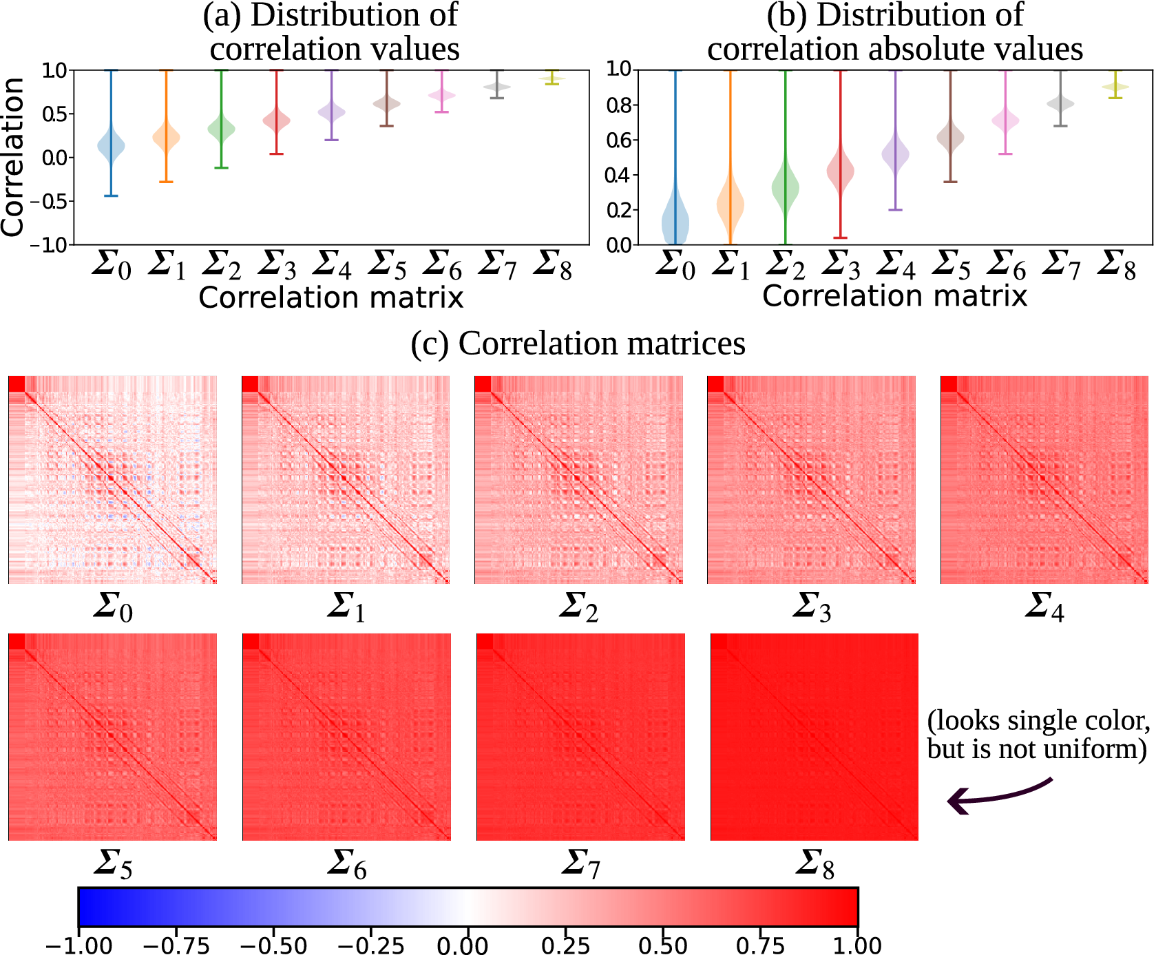
Figure 3. Nine correlation matrices are generated based on the SST anomaly dataset. The pair-wise correlation values are positively shifted to increase overall correlation. The distributions of correlation values are shown in (a) and the absolute values in (b), to confirm that the overall correlation increases even the magnitude of negative correlations are reduced. In (c), the correlation matrices are shown as heatmaps to make it clear that the original relationships are preserved, but their magnitudes shifted.

For each benchmark suite, we train 10 networks using datasets generated from the nine covariance matrices. Since we train networks for each of the four sample sizes, this equals a total of 360 trained models. These trained network repetitions differ only in the training process initializations, each one corresponding to a different random seed to initialize the network weights. Figure 4 provides a comparison of the performance of all networks based on training and validation datasets. In each case, a random selection of 10% of the data is reserved for validation. The reported values are the mean of the 10 trained networks for that benchmark and covariance matrix. The figure shows that network performance improves with the number of training samples, as expected. For the case of using $ {10}^3 $ samples, possible disagreement between the XAI-based and ground truth attributions may be likely due to the networks not capturing the known function as well. With large training samples, especially $ {10}^6 $ , the networks achieve very high performance. In these cases especially, we are interested in seeing how correlations influence the explanations given that the networks effectively capture the target.

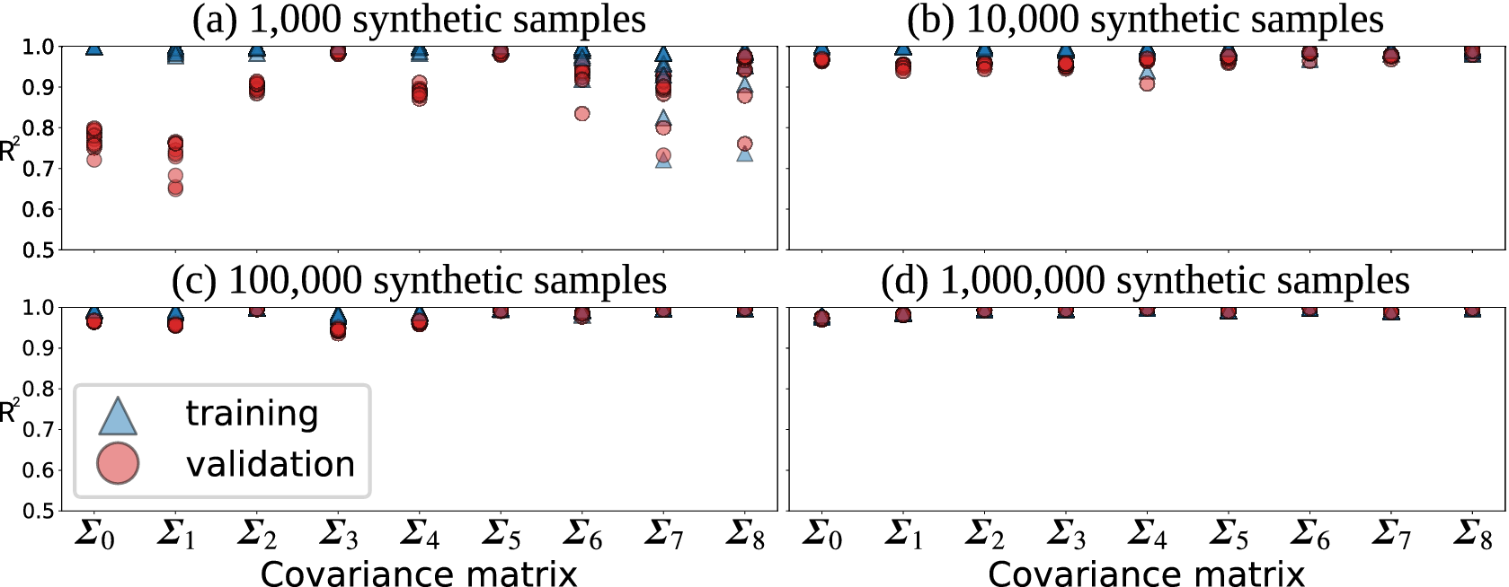
Figure 4. The four benchmarks suites (a–d) each consist of nine datasets generated using nine different covariance matrices (Figure 3). Points represent the mean performance ( $ {R}^2 $ ) for 10 trained networks.

6.2. Pixel-level attributions

We applied the three XAI methods to the 360 trained networks. For each, we used XAI to generate attribution maps for 100 training and 100 validation samples. The analysis of the attribution maps is based mainly on the correlation between them. For each covariance matrix, we calculate the pair-wise correlation between the attributions generated using the 10 trained networks. These attributions are also compared to the synthetic ground truth attributions. This is illustrated in Figure 5 which shows an example comparison between XAI attribution maps and the ground truth for a randomly selected synthetic sample. The top row shows the sample and its ground truth attribution. Below, XAI attributions are shown for the 10 trained networks using the three XAI methods.

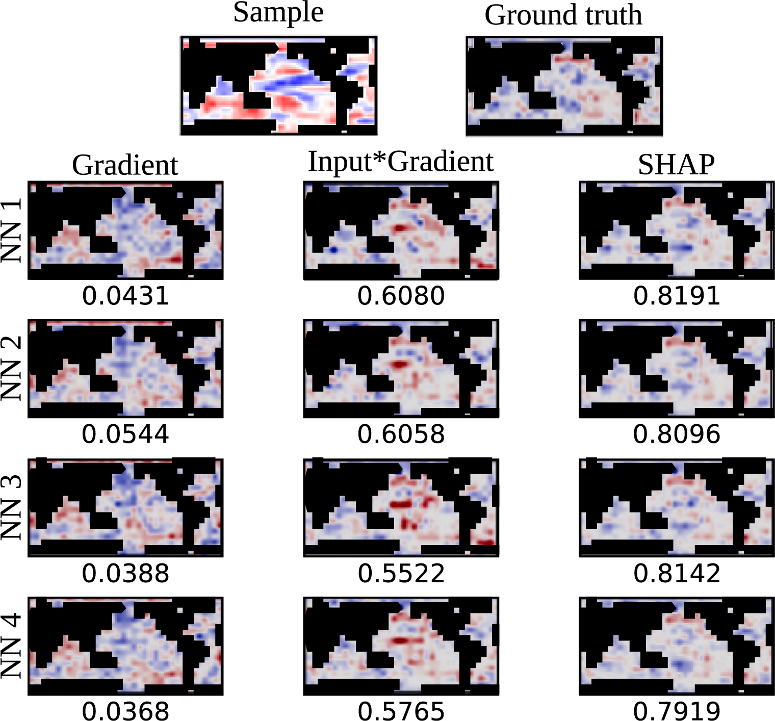
Figure 5. An example of a synthetic SST anomaly sample and its ground truth attribution, along with XAI attributions from three methods. Each sample is initially a 18 $ \times $ 32 raster of synthetic SST anomalies, but the actual input to the network is a flattened vector with the non-ocean pixels (shown here in black) removed. After filtering the non-ocean pixels, each input sample contains $ D $ = 460 features. Ten trained networks are used to generate explanations, and we show samples from four of them here. Below each XAI, attribution is the Pearson correlation between it and the ground truth. This sample is generated from covariance matrix $ {\varSigma}_1 $ , and the networks are trained with $ {10}^6 $ samples.

We also analyze the relationship between the correlation among networks and the correlation with the ground truth. When XAI methods agree, does this suggest that they are all better aligned with the ground truth? In practice, the attribution ground truth is unknown; thus, we are interested in whether the relationship among XAI from trained networks can be used as a proxy to infer the accuracy of the attributions.

We also compute the Faithfulness Correlation, Monotonicity Correlation, and Sparsity metrics for each attribution. We analyze the relationships between these metrics and the correlation among attributions. For brevity, we focus on the Input × Gradient and SHAP results on validation samples. The training samples exhibit very similar characteristics, just with slightly higher correlations overall.

The gradient results are used mainly as a sanity check. We expect the other methods to consistently have a stronger match with the ground truth because Gradient alone is not a true attribution method. Input × Gradient and SHAP consistently align with the ground truth much more closely than Gradient.

Figure 6 summarizes the attribution comparisons using the Input × Gradient XAI method. Figure 6a–d presents the benchmark suites for datasets created using $ {10}^3 $ , $ {10}^4 $ , $ {10}^5 $ , and $ {10}^6 $ synthetic samples, respectively. Examining Figure 6a, there are three panels ( $ \alpha $ , $ \beta $ , and $ \gamma $ ) to analyze attribution correlations for the benchmarks where networks are trained using 1000 synthetic samples. On the left, there are two sets of violin plots (Figure 6a $ \alpha $ and Figure 6a $ \beta $ ). Each violin plot shows the distribution of 1000 correlation values, based on XAI methods applied to 100 validation samples, for the 10 trained networks. The nine violin plots in each panel are based on samples from the nine covariance matrices $ {\boldsymbol{\varSigma}}_0 $ … $ {\boldsymbol{\varSigma}}_8 $ , with increasing covariance strength. Each value making up the distribution is the pairwise Pearson correlation between attributions, for a given sample. In the top-left panel (Figure 6a $ \alpha $ ) each value is the correlation between XAI and the ground truth. This captures how closely the XAI results match the ground truth attribution. In the bottom-left panel (Figure 6a $ \beta $ ), each value is the correlation between XAI attributions generated from each of the 10 trained networks. This captures the variance in attributions from network re-training. Separate violin plots for each covariance matrix are used to analyze how the correlation strength influences the alignment between attributions.

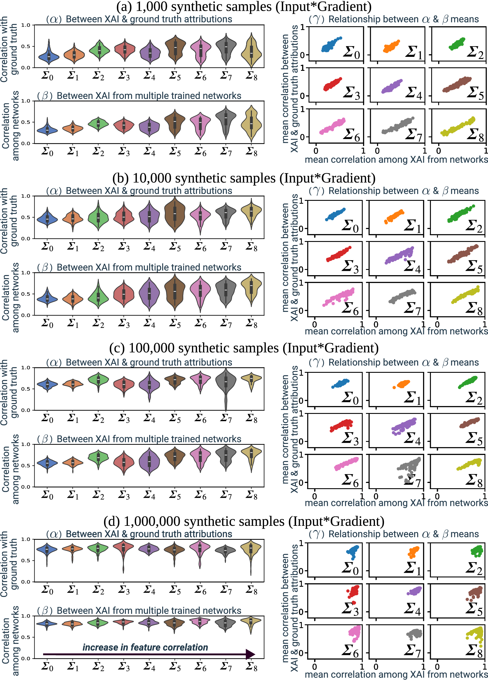
Figure 6. Input × Gradient summary for four benchmark suits (a–d). These correspond to the four sets of synthetic samples, from 10³ (a) to 10⁶ (d). For each, three subpanels are provided to analyze how increasing correlation ( $ {\boldsymbol{\varSigma}}_0 $ … $ {\boldsymbol{\varSigma}}_8 $ ) influences the agreement between the attribution maps. The top-left panel ( $ \alpha $ ) shows the distribution of correlation between XAI-based and ground truth attributions. The bottom-left panel ( $ \beta $ ) shows the distribution of correlation between XAI attributions between trained model repetitions. The left panel ( $ \gamma $ ) compares the alignment in $ \alpha $ and $ \beta $ : for each input sample, the mean correlation between XAI and ground truth is plotted against the mean correlation between the model’s XAI results. The results show that increasing the correlation can substantially increase the variance between XAI attributions, but this is greatly limited with a sufficiently large training set.

The scatterplots on the right panel (Figure 6a $ \gamma $ ) capture, for each covariance matrix $ {\boldsymbol{\varSigma}}_i $ , the relationship between the correlation between XAI and ground truth attributions and the correlation among XAI from the set of networks. That is, the relationship between the network’s agreement with the ground truth and their agreement with each other. For each sample, we calculate the mean pairwise correlations between XAI and ground truth explanations as well as the mean pairwise correlations among the trained networks.

With 1000 training samples (Figure 6a), the mean correlation among attributions does not decrease with increased correlation structure in the input. Initially, we expected to see a decline in mean correlation as the correlation strength grows because more relationships should be available for the network to learn. However, since all correlations are strengthened equally, the original relationships between the inputs and target are preserved (and strengthened as well), which we suspect allows a high-performing network to still identify the best relationships. In fact, the mean correlation initially increases. We suspect this is because the increased correlation smooths out noise in the original dataset by constraining the values to be similar to each other, making it an easier problem for the network to learn.

While correlations do not degrade mean attribution performance, the variance of attribution increases considerably. Consider the sequence of distributions shown in Figure 6a. With $ {\boldsymbol{\varSigma}}_0 $ , there is a relatively narrow bell curve around the mean. With increasing correlation strength, the distribution widens. With $ {\boldsymbol{\varSigma}}_5 $ , the variance increases sharply. Even though the mean agreement between the XAI-based and ground truth attributions has increased, the spread of agreement is very high. The attributions tend to be in a closer alignment with the ground truth, but more poor alignments exist with stronger correlated datasets from $ {\boldsymbol{\varSigma}}_5 $ to $ {\boldsymbol{\varSigma}}_8 $ than with the less correlated datasets from $ {\boldsymbol{\varSigma}}_1 $ to $ {\boldsymbol{\varSigma}}_4 $ .

As the number of training samples increases (Figure 6b–d), the mean correlations tend to increase. This meets expectations since the additional training samples improve network performance, as shown in Figure 4. With a sufficient number of samples, the true relationships are consistently found. That is, the network learns to approximate the designed function, as evidenced by consistently strong correlation between learned attributions and the ground truth (Figure 6d).

In practice, however, we cannot obtain an arbitrarily large sample set in order to identify these relationships. Based on Figure 6a–c, correlation in the input features strongly influences the XAI-based attribution maps in two major ways. First, the mean agreement between XAI and the ground truth may improve. We expect this is because the complexity of the training dataset is reduced by enforcing a consistent structure across the samples, and the network’s prediction performance increases. Thus, this is related to the ability of the network to solve the prediction task (see also results in Figure 4). Second, as the correlation in the input keeps strengthening, another effect appears. Not only the network is able to solve the task, but there are many different patterns to focus on in doing so. Thus, the variance of the agreement between XAI and ground truth increases. In practice, we only have proxies to identify at what point we are in terms of the influence of feature correlation on the attribution. One obvious proxy is the prediction performance of the network to rule out (or not) the possibility that the network has not approximated at all the true underlying function.

Moreover, regardless of the number of training samples, the distribution of correlation among networks and against the ground truth are similar. Since real applications do not have a ground truth, we are interested in using the set of trained networks to infer whether or not the attribution maps are likely to match the true attribution. The approximately linear relationships shown in the scatterplots in Figure 6 ( $ \gamma $ panels) indicate that the higher the agreement among the networks, the closer their attributions are to the ground truth. Thus, checking the correlation among trained networks could potentially be used as another proxy to detect situations where correlated features may be increasing the variance in the attributions and, very likely, in the trained networks themselves, such that users should be cautious in using the derived attributions to learn about the real-world phenomena. Additional work is needed to see if these relationships hold for other input datasets and model architectures.

Figure 7 shows the three XAI evaluation metrics applied to the validation samples: Faithfulness Correlation, Monotonicity Correlation, and Sparseness. Both Faithfulness Correlation and Monotonicity Correlation show an initial slight increase in the faithfulness of attributions to the network, but in general, faithfulness seems to be unaffected by increasingly correlated features. Comparing the metrics on benchmarks using $ {10}^3 $ and $ {10}^6 $ training samples, the influence of correlation on faithfulness is more pronounced with fewer training samples. Here, we cannot conclude that correlations degrade XAI accuracy. Thus, we argue that the increased variance of the correlation between XAI-derived and ground truth attributions is not a result of decreased XAI faithfulness but rather of the fact that the networks are learning different functions from the true one to achieve equally high performance.

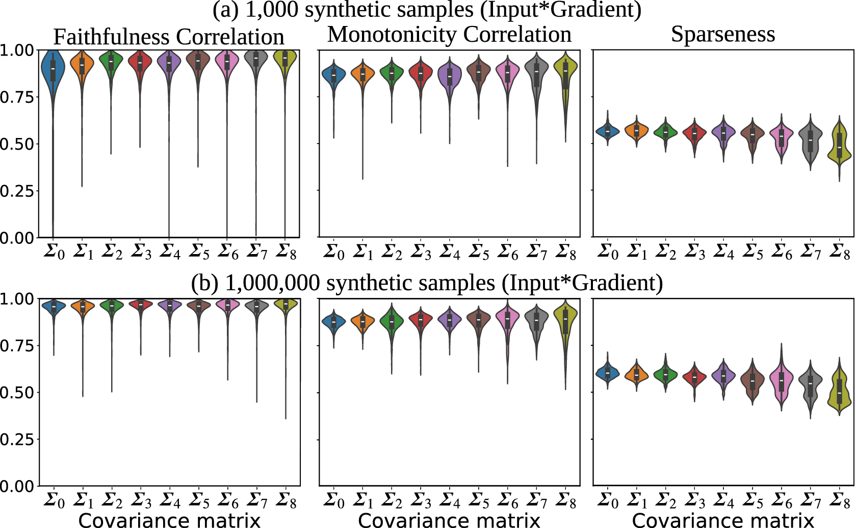
Figure 7. Input × Gradient: XAI evaluation metrics. Faithfulness Correlation and Monotonicity Correlation measure how faithful attributions are to the network, and Sparseness measures attributions’ complexity.

The Sparsity metric in Figure 7 shows that increasing correlation causes the attributions to be more complex. If the attribution values are concentrated in a smaller number of pixels, then the attribution will be sparser. So, the decreasing sparsity suggests that the attributions become spread across a larger number of pixels. Even with an increased number of training samples, the Sparsity metric results suggest that increased correlation can cause the networks to learn more complex functions where many input pixels contribute to the output.

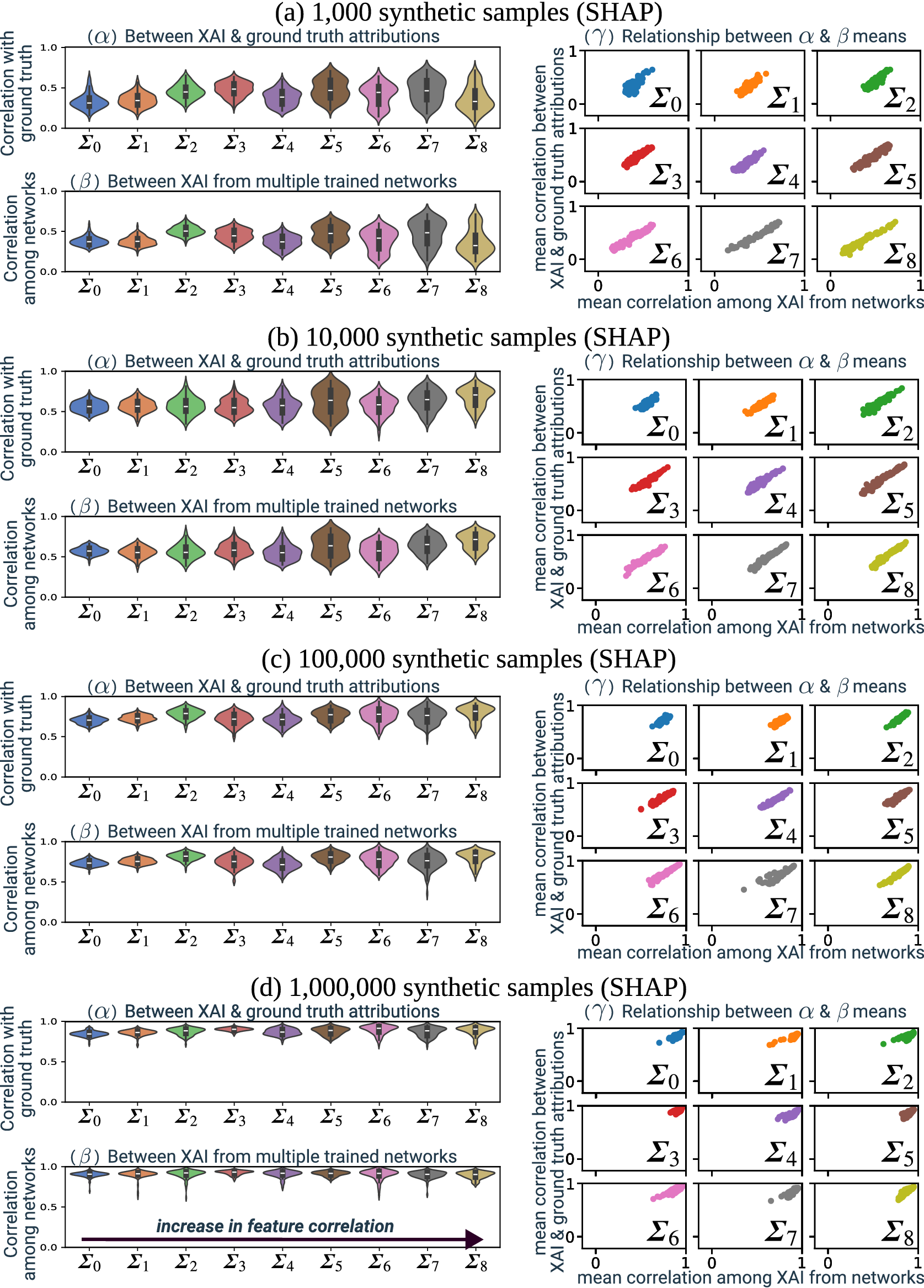
Figure 8. SHAP summary for four benchmark suits (a–d). For each, three subpanels are provided to analyze how increasing correlation ( $ {\boldsymbol{\varSigma}}_0 $ … $ {\boldsymbol{\varSigma}}_8 $ ) influences the agreement between attribution maps. The top-left panel ( $ \alpha $ ) shows the distribution of correlation between XAI-based and ground truth attributions. The bottom-left panel ( $ \beta $ ) shows the distribution of correlation between XAI attributions between trained model repetitions. The left panel ( $ \gamma $ ) compares the alignment in $ \alpha $ and $ \beta $ : for each input sample, the mean correlation between XAI and ground truth is plotted against the mean correlation between the model’s XAI results. The results show that increasing correlation can substantially increase the variance between XAI attributions, but this is greatly limited with a sufficiently large training set.

SHAP results (Figure 8) show very similar characteristics as Input × Gradient. Each SHAP attribution map was generated using 10,000 evaluations. SHAP is a sampling-based approximation of Shapley values, so the results depend on the number of evaluations. Ideally, the SHAP values approach the Shapley values with a sufficiently large number of evaluations. We choose 10,000 evaluations based on experiments with 1000; 5000; 10,000; and 100,000 evaluations. We found that the SHAP results with 1000 and 5000 evaluations were unstable (attributions changed with repeated applications of SHAP). However, the attributions became stable at 10,000 evaluations. Figure 8 presents the correlation analysis for four benchmark suites. Like Input × Gradient, correlated features influence the attributions by expanding the variance in alignment between trained networks and against the ground truth. With $ {10}^6 $ training samples, the networks appear to approximate the synthetic function very closely and achieve near-perfect attribution alignments independently of the degree of correlation in the input. Figure 9 shows the scores for the three XAI evaluation metrics. The overall pattern is similar to that of Input × Gradient, but the faithfulness scores tend to be lower with wider variance.

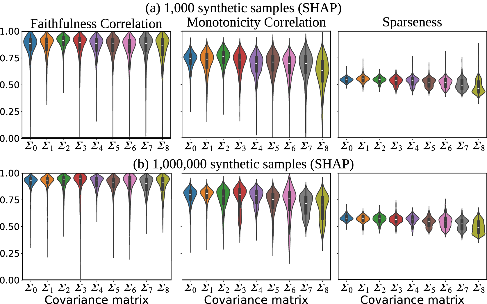
Figure 9. SHAP: XAI evaluation metrics. Faithfulness Correlation and Monotonicity Correlation measure how faithful attributions are to the network, and Sparseness measures their complexity. Each faithfulness metric makes different assumptions to perturb the data (e.g., replacement with 0). Since the results do not vary widely across the two methods, it strengthens our confidence in using the results for our analysis.

Despite the similarity with Input × Gradient, we highlight the SHAP results here for two reasons. First, their strong similarity adds confidence to our analysis and suggests that these attribution experiments reveal insights into how correlated features in spatial data influence attributions. Second, the results show that SHAP is a competitive XAI method. This is important since SHAP is a more general XAI method than Input × Gradient. Attribution maps explain the network’s prediction by showing how each feature leads the network from a baseline value to the network’s prediction. Different baselines can be used to ask different questions about the network, such as which features in the input made the network predict the current output rather than a different baseline value? (Mamalakis et al., 2023). The ground truth attributions correspond to a zero baseline by design. When configuring SHAP, the user provides the baseline. Common choices are maps of all zeros or the mean of each pixel. By choosing an appropriate baseline, SHAP can be configured to investigate a variety of networks and pose different questions. With Input × Gradient, the baseline of 0 is embedded into the method. Thus, Input × Gradient may be appropriate in our task (i.e., for the SST anomaly dataset with a mean of 0), but cannot be as easily tailored for other situations. Mamalakis et al. (2023) provide a detailed investigation into the role of the baseline on attribution methods, highlighting SHAP’s adaptability over Input × Gradient.

6.3. Superpixel attributions

This section presents the results of applying SHAP to create superpixel attribution maps. Superpixel attribution maps are created using two methods. First, by applying SHAP directly to the superpixels. In the preceding sections, all attribution maps are computed by treating individual grid cells (1 × 1 pixels) as features. Instead, here groups of pixels can be treated as features, such as 2 × 2 or 4 × 4 superpixel. The second way is by applying SHAP to only the 1 × 1 pixels and then summing those attribution values into larger superpixels. That is, the 2 × 2 superpixel is simply the sum of four 1 × 1 pixel attributions. Due to the extensive computation required for SHAP results, 4 of the 10 trained models were used. Initial tests show that randomly choosing a subset of models had a negligible impact on the results.

Figure 10 shows the distribution of Pearson correlation between SHAP-derived attributions and the ground truth attribution from $ \mathcal{F} $ for eight different superpixel sizes. We have tested that approximately all correlations are statistically significant (p < 0.1). The superpixels range from the single-pixel (1 × 1) to larger 8 × 8 squares. To visualize how the number of training samples (i.e., samples to fit the network) influences these attributions, Figure 10a,b shows results for $ {10}^3 $ and $ {10}^6 $ samples, respectively. Each subfigure has two plots. On the right, the attributions are generated by applying SHAP to explain each superpixel as a feature. On the left, SHAP was only applied to the 1 × 1 pixels. Superpixel attributions were generated by summation of the 1 × 1 values. While not shown, we observed very similar results based on the correlation among the trained networks instead of against the ground truth attribution. Figure 11 provides an example case with a validation sample from the $ {10}^4 $ sample dataset, generated with covariance matrix $ {\boldsymbol{\varSigma}}_1 $ . The 1 × 1 maps are similar, but the alignment between them improves when using larger superpixels.

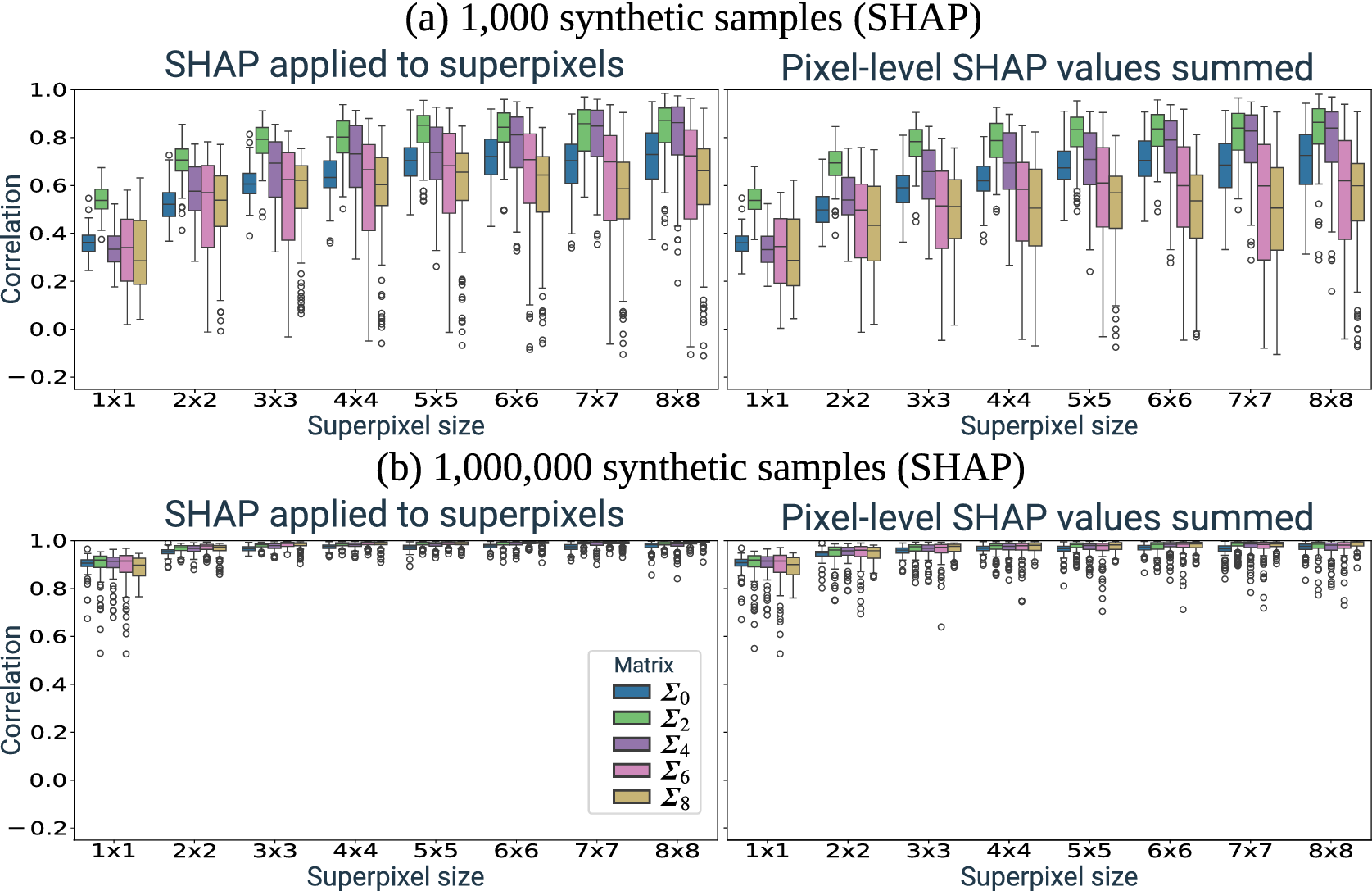
Figure 10. Superpixel XAI for $ {10}^3 $ (a) and $ {10}^6 $ (b) training samples, from 1 × 1 to 8 × 8 patch sizes: the Pearson correlation between SHAP results from NNs $ {\hat{\mathcal{F}}}_1 $ … $ {\hat{\mathcal{F}}}_4 $ with the attribution from $ \mathcal{F} $ . The left-hand plots show correlation when SHAP is applied to each superpixel. The right-hand plots show correlation when superpixels attributions are made by simply summing the 1 × 1 SHAP values.

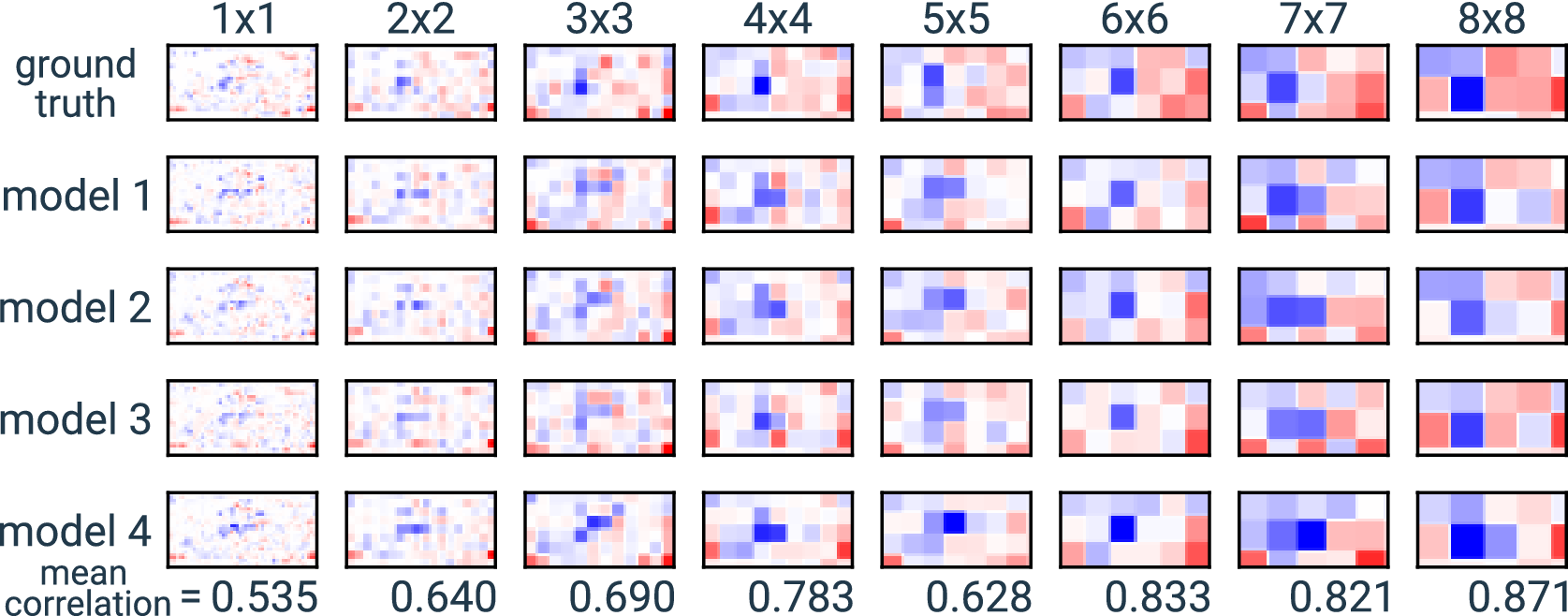
Figure 11. SHAP superpixel attributions (sizes 1 × 1 … 8 × 8) from trained networks $ {\hat{\mathcal{F}}}_1 $ … $ {\hat{\mathcal{F}}}_4 $ are compared to the ground truth attribution from $ \mathcal{F} $ . The networks were trained with $ {10}^4 $ synthetic samples that were generated using covariance matrix $ {\boldsymbol{\varSigma}}_1 $ . The input sample (index 9900 in the supplemental results) was not used during network training. For each superpixel size, we calculate the mean correlation between each SHAP attribution and the ground truth attribution. For the ground truth attributions, superpixel values are calculated by summing the 1 × 1 values. The SHAP attributions are calculated by running SHAP directly on the grouped grid cells.

Based on Figure 10, we make two main observations. First, the correlation between SHAP attributions and the ground truth attribution increases substantially when going from 1 × 1 to 2 × 2 superpixels. This suggests that very localized autocorrelation is a strong driver in attribution differences. That is, the differences between attributions are mostly in small neighborhoods. With autocorrelation, the optimal grid cell used in the synthetic function is surrounded by other, very similar grid cells. So the trained networks can distribute the attribution among that cell’s neighborhood. Comparing Figure 10a,b, it seems that with sufficient samples, the network is more likely to pinpoint the same grid cells as in the synthetic function. Interestingly, the more strongly correlated datasets tend to show an even higher increase in correlation with superpixel-level XAI.

The second observation is the near-identical distributions whether using SHAP or summation-based superpixel attributions. For these benchmarks, there is no advantage to applying SHAP to each superpixel over simply summing the pixel-level SHAP values. The accuracy of SHAP values does not appear to be significantly influenced by correlations. If the correlated pixels were causing the SHAP values to assign poor attributions, then there would be a difference between summation-based and XAI-based superpixel attributions. That is, if derived attributions were inaccurate because of the dependencies in the input, applying SHAP on the group of dependent features would result in different attributions than applying to individual ones and then adding them up. Thus, here, differences between the attributions are largely driven by actual differences in what the 10 trained networks learned, rather than correlated features degrading the accuracy of SHAP (see also remarks about Figure 9). Note that this is not always the case, as demonstrated in the XAI analysis of FogNet (Krell et al., 2023). In that study, we observed major differences between attributions calculated across different scales of the high-dimensional raster input. Results overall show that correlation in the input may significantly influence what the network learns and consequently the XAI results (inflating the corresponding variance) and physical insights. The predictive performance and the agreement of XAI results among different trained networks can be used to assess the degree to which the network and XAI results capture the true underlying function when no ground truth is provided. Finally, applying XAI to superpixels may be used as an approach to increase certainty and address the inflated variance of the explanations.

7. Conclusions and future work

It is commonly assumed that correlated features influence XAI, but their actual impact on attributions is under-explored. We proposed a novel framework for investigating how correlated features influence the XAI attributions for a geophysical model. Building on the synthetic benchmark framework proposed in Mamalakis et al. (2022a), we built a suite of benchmarks by inducing stronger correlation in a covariance matrix estimated from real-world geospatial data.

We found that stronger correlations did not lead to an average decrease in the agreement between the XAI attributions and the attributions derived from the synthetic function (the ground truth). However, the variance of XAI results increases significantly. Attributions may be influenced by correlations in two main ways: (1) by compromising XAI faithfulness, that is, XAI less accurately detects the true attributions, or (2) by increasing the number of available combinations of patterns/strategies for the network to learn. In this study, we were able to provide evidence that suggest that the XAI-based attributions are approximately accurate. Instead, the high XAI variance appears to be largely driven by differences in what the models have learned. With this in mind, we can be more confident in studying the pixel-level XAI results for each trained model to determine what they learned. We can also aggregate the results to potentially gain insights into the real-world phenomena. With small superpixel sizes (e.g., 2 × 2, 3 × 3), the attributions are less sensitive to very minor differences in the trained models to show a clearer picture on learned strategies.

Using $ {R}^2 $ to measure global model performance, we observed that larger training datasets yield higher model performance. We also observed that higher-performance models yield stronger correlations between the ground truth and XAI-based attributions. This suggests that the higher-performance models are better approximations of the known function. However, the distributions reveal that even with $ {R}^2 $ approaching 1.0, there is still imperfect alignment between the ground truth and XAI-based attributions. While our results strongly suggest that this difference is influenced by the presence of correlated features, we recognize that some individual cases may not be well captured: erroneous predictions such that the XAI-based attributions should differ from the ground truth since the model did not learn the function in that case. However, we believe that the relationships among input size, input correlation, and attribution agreement provided compelling evidence that correlation in the input domain allows models to learn a variety of functional relationships. With larger input datasets, the models better approximate the known function, resulting in tight distributions of high alignment between ground truth and XAI-based attributions, despite strong correlation in the input domain.

This research provides a framework for investigating models. By training several models, XAI practitioners can apply several of our methods to get an idea of the impact of correlated features on their results. For example, by performing superpixel XAI to test the sensitivity of the attributions. More work is required to study the influence of correlated features on geophysical models. It would be very useful to repeat this study on similar datasets to test the generalization of our observations. We expect our methodology and findings to be broadly applicable to a variety of applications across geoscience fields, including climatology, hydrology, and ecology. Especially, the characteristics of the SST anomaly dataset are highly relevant to many applications dealing with high-variability systems influenced by human action and climate change. By repeating this methodology with other datasets, researchers can assess if their datasets achieve similar results.

We are also interested in additional ways of varying the input correlation. To isolate the correlation variance to a single parameter, we increased the overall correlation (all pairwise correlations positively increased). Instead, we could generate synthetic data in other ways to add strong correlation across certain image regions (e.g., induce a strong teleconnection). We are also interested in experimenting with the number of input features ( $ D $ ). With more features, there are more opportunities for correlation among features. However, there is a particular concern we have with the spatial resolution of geospatial data. Here, the synthetic SST is represented by a coarse resolution. With finer-scale gridded data, the same spatial patterns are captured with more information. Thus, the spatial autocorrelation tends to depend strongly on the spatial resolution. We are interested in experiments where benchmarks are produced using a sequence of finer to coarser resolution inputs.

Finally, we highlight that some of our results and conclusions may be dependent on the form of the function $ \mathcal{F} $ (a separable additive function) and the network architecture used here to train and approximate $ \hat{\mathcal{F}} $ . In particular, we are interested in comparing our results to those using CNN-based networks. With MLP, each feature can be semantically meaningful. With convolutions, the grid cells are combined into features; thus, pixel-level XAI may struggle with CNN-based models since each pixel has less information when permuted in isolation.