


1 Introduction
The classification of holomorphic univariate parabolic germs up to local change of analytic coordinate was first described by Birkhoff [Reference BirkhoffBir39] in 1939, but the manuscript was somehow forgotten almost immediately to be rediscovered only by the end of the century. In the meantime, Écalle [Reference ÉcalleÉca75] and Voronin [Reference VoroninVor81] carried out this task again nearly forty years ago. In addition to building a modulus (characterizing the conjugacy class of a parabolic germ), they were able to solve the inverse problem by recognizing which similar objects came as the moduli of parabolic germs, a property G. Birkhoff was only able to conjecture. The latter problem is what interests us in the present paper.
1.1 Modulus of classification and inverse problem
Heuristically, if $\Delta $
is a germ that is tangent to the identity and fixes
$\Delta $
is a germ that is tangent to the identity and fixes $0\in \mathbb {C}$
,
$0\in \mathbb {C}$
,
then the conformal structure of its orbit space $\Omega $
completely encodes its analytic class up to local changes of analytic coordinate near the fixed point. For the sake of simplicity, assume that
$\Omega $
completely encodes its analytic class up to local changes of analytic coordinate near the fixed point. For the sake of simplicity, assume that $\Delta $
is generic, that is, that it belongs to the space
$\Delta $
is generic, that is, that it belongs to the space
(here and in everything that follows, $*$
stands for a non-zero complex number).
$*$
stands for a non-zero complex number).
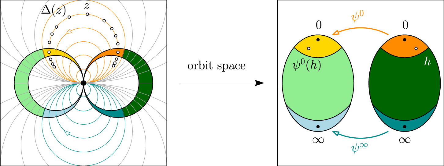
Figure 1 Fundamental region of the dynamics of a generic parabolic germ (left) and the corresponding orbit space and horn maps (right) (colour online).
It is well known that a fundamental region for the iterative action of $\Delta $
is given by a pair of crescent-shaped regions that are identified by the dynamics near their horns, attached at the fixed point
$\Delta $
is given by a pair of crescent-shaped regions that are identified by the dynamics near their horns, attached at the fixed point $0$
. More precisely, as dipicted in Figure 1, the orbit space
$0$
. More precisely, as dipicted in Figure 1, the orbit space
is obtained as the gluing of two spheres $\overline {\mathbb {C}}$
near
$\overline {\mathbb {C}}$
near $0$
and
$0$
and $\infty $
by germs of a diffeomorphism
$\infty $
by germs of a diffeomorphism ![]() and
and ![]() , sometimes called horn maps:
, sometimes called horn maps:
When we endow the space ![]() with the quotient topology, the two points
with the quotient topology, the two points $0$
and
$0$
and $\infty $
(corresponding to the fixed point of
$\infty $
(corresponding to the fixed point of $\Delta $
) are not separated.
$\Delta $
) are not separated.
One can choose conformal coordinates on the spheres so that ![]() itself becomes tangent to the identity. The only degree of freedom that remains is the linear change of coordinates
itself becomes tangent to the identity. The only degree of freedom that remains is the linear change of coordinates $h\mapsto ch$
for
$h\mapsto ch$
for $c\in \mathbb {C}^{\times }$
applied simultaneously to both spheres. The Birkhoff–Écalle–Voronin (BÉV) theorem (see aforementioned bibliography) states that the map
$c\in \mathbb {C}^{\times }$
applied simultaneously to both spheres. The Birkhoff–Écalle–Voronin (BÉV) theorem (see aforementioned bibliography) states that the map
is well defined and one-to-one. The Écalle–Voronin theorem states that it is also onto, answering the inverse problem.
Problem. Being given a pair ![]() , recover (synthesize) a parabolic germ
, recover (synthesize) a parabolic germ $\Delta $
such that its modulus is
$\Delta $
such that its modulus is ![]() .
.
In the present article, we revisit the question and provide an essentially unique representative $\Delta $
for a given pair
$\Delta $
for a given pair ![]() , what can be called a normal form. The germ
, what can be called a normal form. The germ $\Delta $
will be ‘global’ on the sphere
$\Delta $
will be ‘global’ on the sphere $\overline {\mathbb {C}}$
in some sense, which is why we borrow Écalle’s terminology and speak about spherical normal forms.
$\overline {\mathbb {C}}$
in some sense, which is why we borrow Écalle’s terminology and speak about spherical normal forms.
1.2 Statement of the main results
We answer the inverse problem in the following fashion.
Synthesis Theorem. For fixed $\mu \in \mathbb {C}$
and positive
$\mu \in \mathbb {C}$
and positive $\unicode{x3bb}>0$
, define the rational vector field (holomorphic near
$\unicode{x3bb}>0$
, define the rational vector field (holomorphic near $0$
and
$0$
and $\infty $
), called here the formal model,
$\infty $
), called here the formal model,
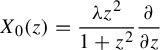
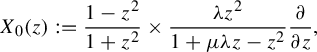 $$ \begin{align*} X_{0}(z) :=\frac{1-z^{2}}{1+z^{2}}\times\frac{\unicode{x3bb} z^{2}}{1+\mu\unicode{x3bb} z-z^{2}}\frac{\partial}{\partial z}, \end{align*} $$
and denote by $f\mapsto X_{0}\cdot f$
the associated Lie (directional) derivative on a power series. Let
$f\mapsto X_{0}\cdot f$
the associated Lie (directional) derivative on a power series. Let ![]() be given and pick
be given and pick $\mu $
so that
$\mu $
so that ![]() .
.
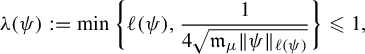
One can then find an explicit $\unicode{x3bb} (\psi )>0$
such that for each
$\unicode{x3bb} (\psi )>0$
such that for each $0<\unicode{x3bb} \leq \unicode{x3bb} (\psi )$
, there exists a unique formal power series
$0<\unicode{x3bb} \leq \unicode{x3bb} (\psi )$
, there exists a unique formal power series $F\in z\mathbb {C}[[z]] $
, depending on
$F\in z\mathbb {C}[[z]] $
, depending on $\unicode{x3bb} $
and satisfying all of the following properties.
$\unicode{x3bb} $
and satisfying all of the following properties.
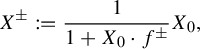
-
(1) The time- $1$
map
$\Delta $
of the formal vector field, said to be in spherical normal form, is a convergent power series at
$$ \begin{align*} X_{F}:= \frac{1}{1+X_{0}\cdot F}X_{0}, \end{align*} $$
$0$
(that is, with positive radius of convergence).
$1$
map
$\Delta $
of the formal vector field, said to be in spherical normal form, is a convergent power series at
$$ \begin{align*} X_{F}:= \frac{1}{1+X_{0}\cdot F}X_{0}, \end{align*} $$
$0$
(that is, with positive radius of convergence).
-
(2)
$\Delta $
belongs to with -
(3) The power series F is
$1$
-summable (see below) and its 1-sum can be realized as a pair
$(f^{+},f^{-})$
of functions holomorphic and bounded by
$1$
on the respective infinite sectors as in Figure 2.
$$ \begin{align*} V^{\pm} :=\bigg\{ z\neq0:\lvert\ \arg(\pm z)\rvert<\frac{5\pi}{8}\bigg\} \end{align*} $$
Figure 2 The infinite sectors
$V^{\pm }$
and the components , of their intersection
$V^{\cap }$
(colour online).


A pair $f=(f^{+},f^{-})$
of functions holomorphic on the corresponding sector
$f=(f^{+},f^{-})$
of functions holomorphic on the corresponding sector $V^{+}$
or
$V^{+}$
or $V^{-}$
has order-1 flat discrepancy at
$V^{-}$
has order-1 flat discrepancy at $0$
whenever
$0$
whenever
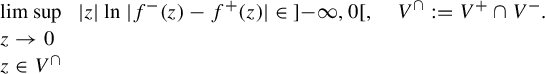 $$ \begin{align*} \limsup_{\begin{array}{l} z\to0\\ z\in V^{\cap} \end{array}}|z|\ln|f^{-}(z)-f^{+}(z)|\in\ ]{-}\infty,0[, \quad V^{\cap}:=V^{+}\cap V^{-}. \end{align*} $$
It follows from a theorem of Ramis and Sibuya [Reference Loday-RichaudLR16, Theorem 5.2.1] that there exists some $F=\sum _{n\geq 0}F_{n}z^{n}\in \mathbb {C}[[z]] $
, which is their common Gevrey-1 asymptotic expansion at
$F=\sum _{n\geq 0}F_{n}z^{n}\in \mathbb {C}[[z]] $
, which is their common Gevrey-1 asymptotic expansion at $0$
(in the sense of Poincaré):
$0$
(in the sense of Poincaré):
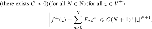 $$ \begin{align*} (\text{there exists } C>0)&(\text{for all } N\in\mathbb{N}) (\text{for all } z\in V^{\pm})\\&\bigg|f^{\pm}(z)-\sum_{n>0}^{N}F_{n}z^{n}\bigg|\leq C(N+1)!|z|^{N+1}. \end{align*} $$
We then say that F is $1$
-summable with
$1$
-summable with $1$
-sum f. The mapping
$1$
-sum f. The mapping $f\mapsto F$
is injective (because
$f\mapsto F$
is injective (because $V^{\pm }$
is wider than a half-plane). This notion is compatible with the usual arithmetic and differential operations (by taking a narrower subsector if necessary).
$V^{\pm }$
is wider than a half-plane). This notion is compatible with the usual arithmetic and differential operations (by taking a narrower subsector if necessary).
Remark 1.1. The notion of $*$
-summability has a standard, more general definition (see e.g. [Reference Loday-RichaudLR16]) allowing for more flexibility. We will not need the whole refinement of the theory as we only rely on this specific implementation of the theorem of Ramis and Sibuya.
$*$
-summability has a standard, more general definition (see e.g. [Reference Loday-RichaudLR16]) allowing for more flexibility. We will not need the whole refinement of the theory as we only rely on this specific implementation of the theorem of Ramis and Sibuya.
We can exhibit a value of the upper bound $\unicode{x3bb} (\psi )$
as follows. There exist
$\unicode{x3bb} (\psi )$
as follows. There exist $\mathfrak {m}_{\mu },\mathfrak {t}_{\mu }>0$
depending only on
$\mathfrak {m}_{\mu },\mathfrak {t}_{\mu }>0$
depending only on $\mu $
(given for instance in equation (4.2)) for which, if we denote by
$\mu $
(given for instance in equation (4.2)) for which, if we denote by ![]() and
and ![]() the respective radii of convergence of the Taylor series at
the respective radii of convergence of the Taylor series at $0$
of
$0$
of ![]() and
and ![]() , we may define
, we may define
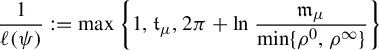
and take
where
Remark 1.2.
-
(1) Any holomorphic vector field X with a double zero at
$0$
is the infinitesimal generator of a generic parabolic germ with modulus
$({e}^{4\pi ^{2}\mu }\mathrm {Id},\mathrm {Id})$
for some
$\mu \in \mathbb {C}$
, see [Reference ÉcalleÉca75]. In this case, we say that the modulus is trivial. This is, in particular, the case for
$X_{0}$
. As a consequence of the uniqueness assertion above, the only normal form with convergent
$F\in z\mathbb {C}[[z]] $
is the formal model itself (
$F=0$
). -
(2) Let
$X\in z^{2}(\mathbb {C}^{\times }+z\mathbb {C}[[z]] ){\partial }/{\partial z}$
be a formal vector field with a double zero at
$0$
. It may happen that the formal power series is convergent at
$$ \begin{align*} \Delta :=(\exp X)\cdot\mathrm{Id} \end{align*} $$
$0$
, in which case, it belongs to and we say that
$\Delta $
is the time-1 map of the infinitesimal generator X. Beware that this does not imply the convergence of
$(\exp tX)\cdot \mathrm {Id}$
for
$t\notin \mathbb {Z}$
even for small
$|t|$
: this is, for instance, the case with the entire map
$\Delta :z\mapsto \exp (z)-z$
(see [Reference BakerBak62]). If the lattice of those
$t\in \mathbb {C}$
for which the power series converges is not discrete, then the modulus of
$\Delta $
is trivial [Reference ÉcalleÉca75] (that is,
$\Delta $
is analytically conjugate to the time-1 flow of a vector field holomorphic near 0).
-
(3) There might exist other representatives of
of the form
$({1}/({1+X_{0}\cdot F}))X_{0}$
for some
$1$
-summable F with
$1$
-sum f on
$V^{\pm }$
. Then, f must have large norm. This is likely related to what F. Loray discusses after [Reference LorayLor04, Theorem 1].


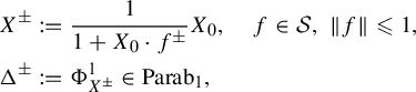
The functions $z\in V^{\pm }\mapsto f^{\pm }(z)-(({1-z^{2}})/{\unicode{x3bb} z})+\mu \log ({\unicode{x3bb} z}/({1-z^{2}}))$
are Fatou coordinates for
$z\in V^{\pm }\mapsto f^{\pm }(z)-(({1-z^{2}})/{\unicode{x3bb} z})+\mu \log ({\unicode{x3bb} z}/({1-z^{2}}))$
are Fatou coordinates for $\Delta $
(that is, local conformal coordinates
$\Delta $
(that is, local conformal coordinates ![]() on which
on which $\Delta $
acts as a translation by
$\Delta $
acts as a translation by $1$
, see §3.2). Hence, we parametrize the analytic classes of parabolic germs by their formal Fatou coordinates. By picking them in a class of ‘global’ formal objects, we benefit from a rigidity which makes the parametrization injective.
$1$
, see §3.2). Hence, we parametrize the analytic classes of parabolic germs by their formal Fatou coordinates. By picking them in a class of ‘global’ formal objects, we benefit from a rigidity which makes the parametrization injective.
The power series F is global in the sense that its $1$
-sum
$1$
-sum $f=(f^{+},f^{-})$
exists on a pair of sectors whose union covers
$f=(f^{+},f^{-})$
exists on a pair of sectors whose union covers $\mathbb {C}^{\times }$
. Moreover,
$\mathbb {C}^{\times }$
. Moreover, $\Delta |_{V^{\pm }}$
is the time-1 map of the
$\Delta |_{V^{\pm }}$
is the time-1 map of the $1$
-sum of its formal infinitesimal generator
$1$
-sum of its formal infinitesimal generator
 $$ \begin{align*} X_{}^{\pm} :=\frac{1}{1+X_{0}\cdot f^{\pm}}X_{0}, \end{align*} $$
which is a meromorphic vector field on $V^{\pm }$
. A quick computation tells us that the formal model
$V^{\pm }$
. A quick computation tells us that the formal model $X_{0}$
is invariant by the involution
$X_{0}$
is invariant by the involution
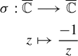 $$ \begin{align*} \sigma:\overline{\mathbb{C}} & \longrightarrow\overline{\mathbb{C}}\\ z & \mapsto\frac{-1}{z} \end{align*} $$
fixing $\pm {i}$
, while the sectors
$\pm {i}$
, while the sectors $V^{+}$
and
$V^{+}$
and $V^{-}$
are swapped, that is,
$V^{-}$
are swapped, that is,
 $$ \begin{align*} \sigma(V^{\pm}) =V^{\mp}. \end{align*} $$
A nice feature of the synthesis is that f not only defines a parabolic germ near $0$
, but it also creates one at
$0$
, but it also creates one at $\infty $
, corresponding to the companion dynamics induced there by
$\infty $
, corresponding to the companion dynamics induced there by $X^{\pm }$
, since (§4.3)
$X^{\pm }$
, since (§4.3)
 $$ \begin{align} f^{\pm}\circ\sigma =-f^{\mp}. \end{align} $$
This is why we call these dynamical systems spherical normal forms, a term borrowed from Écalle [Reference EcalleEca05] as discussed in §1.2.2. We can describe completely the dynamics of $\Delta $
and its monodromy as a multivalued map over the whole Riemann sphere
$\Delta $
and its monodromy as a multivalued map over the whole Riemann sphere $\overline {\mathbb {C}}$
.
$\overline {\mathbb {C}}$
.
Globalization Theorem. Assume $\mu \neq 0$
.
$\mu \neq 0$
.
-
(1) If
$\unicode{x3bb} <\min \{ {1}/{2|\mu |}, {1}/{12\,800}\} $
, then
$X_{}^{\pm }$
has exactly three (simple) poles
$\{ p_{-{i}},p_{{i}},p_{\pm }\} $
, which are
$\mathrm {O}(\sqrt {\unicode{x3bb} })$
-close to
$-{i}$
,
${i}$
and
$\pm 1$
, respectively. In particular, this means that the pole
$p_{\pm {i}}$
is shared by
$X^{-}$
and
$X^{+}$
. -
(2) (See Figure 3.) To each one of the four poles
$p\in \{ p_{-{i}},p_{{i}},p_{-},p_{+}\} $
is attached a unique pair of
$\mathrm {O}(\sqrt {\unicode{x3bb} })$
-close points
$\{ z_{p},w_{p}\} $
lying at the intersection of the stable manifolds through p of
$X_{f}^{+}$
and
$X_{f}^{-}$
, mapped onto p by the time-1 map of
$X_{f}^{\pm }$
. In other words, the analytic continuation of
$\Delta $
to
$\overline {\mathbb {C}}$
provides a multivalued map with ramification points at each
$z_{p}$
and
$w_{p}$
, to which it extends continuously by
$\Delta (z_{p})=\Delta (w_{p})=p$
. A domain of holomorphy for
$\Delta $
is given, for instance, by the slit sphere where
$$ \begin{align*} \mathcal{D}:= \overline{\mathbb{C}}\backslash\bigcup_{p\text{ pole}}\gamma_{p}, \end{align*} $$
$\gamma _{p}$
is the arc of stable manifold passing through p of
$X_{f}^{+}$
or
$X_{f}^{-}$
(choose one) linking
$z_{p}$
and
$w_{p}$
. In particular, the radius of convergence about
$0$
of
$\Delta $
is
$1+\mathrm {O}(\sqrt {\unicode{x3bb} })$
.Figure 3 Foliation induced by the real-time flow of a typical sectorial vector field
$X^{+}$
with the highlighted six ramification points
$z_{p}$
,
$w_{p}$
(orange spots) of its time-1 map
$\Delta $
. The poles
$p_{- {i}},p_{ {i}},~p_{+}$
of
$X^{+}$
are represented by red squares (colour online). -
(3) The multivalued continuation of
$\Delta $
to
$\overline {\mathbb {C}}$
has eight branch points. The monodromy around any one of the eight points
$\{ z_{p},~w_{p}:p\in \{ p_{-{i}},p_{{i}},p_{-},p_{+}\} \} $
is involutive. -
(4)
$\Delta |_{\mathcal {D}}$
is holomorphic and injective. It possesses four fixed-points
$0$
,
$\infty $
and
$\pm 1$
. The first two are parabolic, while
$\Delta $
admits a linearizable dynamics at
$\pm 1$
of multiplier
$\exp (\mp {1}/{\mu })$
. The dynamics at infinity
$\sigma ^{*}\Delta =\sigma \circ \Delta \circ \sigma $
belongs to and
$$ \begin{align*} \mathrm{B}\acute{\mathrm{E}}\mathrm{V}(\sigma^{*}\Delta) =\mathrm{B}\acute{\mathrm{E}}\mathrm{V}(\Delta)^{\circ-1}. \end{align*} $$


In the case where $\mu =0$
, the result still holds except that the pole
$\mu =0$
, the result still holds except that the pole $z_{\pm }$
near
$z_{\pm }$
near $\pm 1$
cancels out the stationary point at
$\pm 1$
cancels out the stationary point at $\pm 1$
. There only remain the parabolic fixed-points of
$\pm 1$
. There only remain the parabolic fixed-points of $\Delta $
and its ramification locus coming from
$\Delta $
and its ramification locus coming from $\{ -{i},{i}\} $
.
$\{ -{i},{i}\} $
.
It is remarkable that a twin fixed-point is automatically produced at $\infty $
, especially because the modulus there is given by the reciprocal modulus. This has a simple explanation, however: the involution
$\infty $
, especially because the modulus there is given by the reciprocal modulus. This has a simple explanation, however: the involution $\sigma $
permutes the sectors
$\sigma $
permutes the sectors $V^{+}$
and
$V^{+}$
and $V^{-}$
, while it does not change the infinitesimal generators much; therefore, the identification at the horns is the same while taking place in the reverse direction.
$V^{-}$
, while it does not change the infinitesimal generators much; therefore, the identification at the horns is the same while taking place in the reverse direction.
Another remarkable feature is that $\Delta $
has very simple dynamics: it is an injective, holomorphic map on a slit sphere
$\Delta $
has very simple dynamics: it is an injective, holomorphic map on a slit sphere $\mathcal {D}$
that can be forward iterated on the open set
$\mathcal {D}$
that can be forward iterated on the open set $\overline {\mathbb {C}}\backslash \gamma $
, where
$\overline {\mathbb {C}}\backslash \gamma $
, where $\gamma $
is the union of the closure of the stable manifolds of
$\gamma $
is the union of the closure of the stable manifolds of $X^{\pm }$
passing through the poles. On each connected component of
$X^{\pm }$
passing through the poles. On each connected component of $\overline {\mathbb {C}}\backslash \gamma $
, the dynamics of
$\overline {\mathbb {C}}\backslash \gamma $
, the dynamics of $\Delta $
converges uniformly to a fixed-point (a parabolic point or the attracting point sitting at
$\Delta $
converges uniformly to a fixed-point (a parabolic point or the attracting point sitting at $\pm 1$
when
$\pm 1$
when $\mu \notin {i}\mathbb {R}$
). The reason behind this stable behaviour is the parameter
$\mu \notin {i}\mathbb {R}$
). The reason behind this stable behaviour is the parameter $\unicode{x3bb} $
, which is chosen so that no chaotic remains of a global dynamics, usually arising from a frontier in the analytic continuation of the modulus [Reference EpsteinEps93], can be seen from the normal form.
$\unicode{x3bb} $
, which is chosen so that no chaotic remains of a global dynamics, usually arising from a frontier in the analytic continuation of the modulus [Reference EpsteinEps93], can be seen from the normal form.
The obvious downside of the previous feature is precisely that the dynamics of $\Delta $
is too simple to readily offer an insight regarding the dynamical richness that is displayed by holomorphic iteration on compact curves. What we prove is that any such dynamics, say of a rational mapping with a parabolic basin
$\Delta $
is too simple to readily offer an insight regarding the dynamical richness that is displayed by holomorphic iteration on compact curves. What we prove is that any such dynamics, say of a rational mapping with a parabolic basin $\mathcal {B}$
, is locally conjugate by some
$\mathcal {B}$
, is locally conjugate by some $\Psi $
to a spherical normal form near the parabolic fixed-point
$\Psi $
to a spherical normal form near the parabolic fixed-point $0$
, but the domain of the conjugacy cannot contain the whole component
$0$
, but the domain of the conjugacy cannot contain the whole component $\partial \mathcal {B}$
of the Julia set. Indeed,
$\partial \mathcal {B}$
of the Julia set. Indeed, ![]() can be pushed forward by the flow of
can be pushed forward by the flow of $X^{+}$
to give a compact invariant set J which is locally conformally equivalent to the fractal set
$X^{+}$
to give a compact invariant set J which is locally conformally equivalent to the fractal set $\partial \mathcal {B}$
. However, the one set J has no relevance to the dynamics of
$\partial \mathcal {B}$
. However, the one set J has no relevance to the dynamics of $\Delta $
whatsoever, for the latter has only Fatou components with real-analytic boundary, and that regularity increases as
$\Delta $
whatsoever, for the latter has only Fatou components with real-analytic boundary, and that regularity increases as $\unicode{x3bb} \to 0$
. In that respect, an interesting question arises: can one recover part of the original dynamics by letting
$\unicode{x3bb} \to 0$
. In that respect, an interesting question arises: can one recover part of the original dynamics by letting $\unicode{x3bb} $
grow (which may cause
$\unicode{x3bb} $
grow (which may cause $X^{\pm }$
to sport more and more poles, for instance)?
$X^{\pm }$
to sport more and more poles, for instance)?
1.2.1 Regarding the formal model
The family of vector fields $X_{0}$
depending on
$X_{0}$
depending on $\unicode{x3bb}>0$
is obtained from the ‘usual’ formal model
$\unicode{x3bb}>0$
is obtained from the ‘usual’ formal model $({x^{2}}/({1+\mu x}))({\partial }/{\partial x})$
(see Figure 4) by performing the degree-2 pullback
$({x^{2}}/({1+\mu x}))({\partial }/{\partial x})$
(see Figure 4) by performing the degree-2 pullback
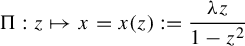 $$ \begin{align*} \Pi:z \mapsto x=x(z):=\frac{\unicode{x3bb} z}{1-z^{2}} \end{align*} $$
(which is invertible near $0$
). Observe that
$0$
). Observe that $\Pi $
is invariant under the involution
$\Pi $
is invariant under the involution $\sigma $
, so that
$\sigma $
, so that $\sigma $
is a symmetry of
$\sigma $
is a symmetry of $X_{0}$
, a fact that has been already remarked. The obvious consequence is that
$X_{0}$
, a fact that has been already remarked. The obvious consequence is that $X_{0}$
has a stationary point at
$X_{0}$
has a stationary point at $\infty $
that mirrors the one it admits at
$\infty $
that mirrors the one it admits at $0$
.
$0$
.
Remark 1.3. The only normal form $X_{f}$
that can be factored through
$X_{f}$
that can be factored through $\Pi $
(that is, realized as a global sectorial perturbation of the usual formal model) is the formal model itself (
$\Pi $
(that is, realized as a global sectorial perturbation of the usual formal model) is the formal model itself ( $f=0$
) since we must both have
$f=0$
) since we must both have $f^{\pm }\circ \sigma =f^{\mp }$
(factorization through
$f^{\pm }\circ \sigma =f^{\mp }$
(factorization through $\Pi $
) and
$\Pi $
) and $f^{\pm }\circ \sigma =-f^{\mp }$
as in equation (1.1).
$f^{\pm }\circ \sigma =-f^{\mp }$
as in equation (1.1).
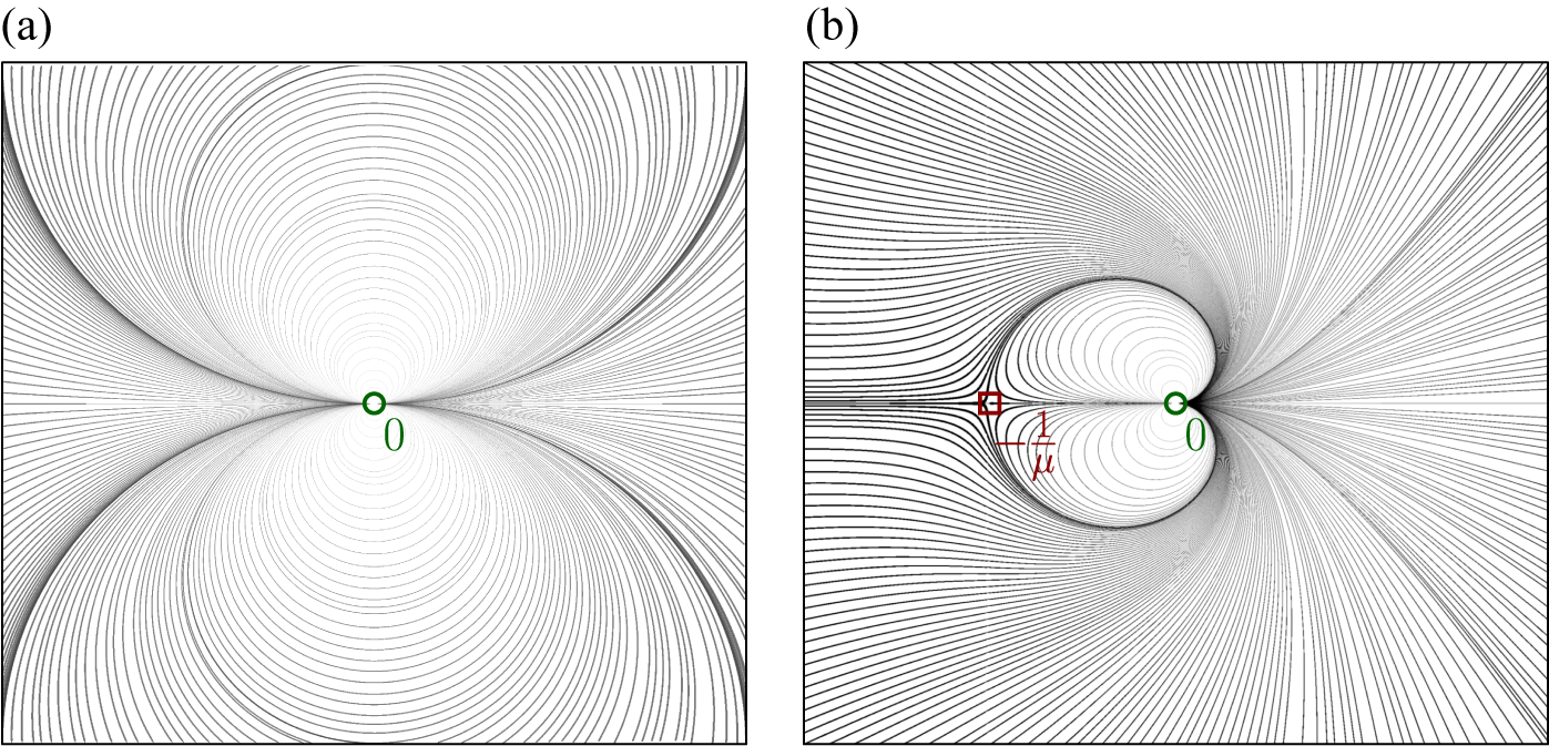
Figure 4 Foliation induced by the real-time flow of $({x^{2}}/({1+\mu x})) {\partial }/{\partial x}$
((a)
$({x^{2}}/({1+\mu x})) {\partial }/{\partial x}$
((a) $\mu :=0$
; (b),
$\mu :=0$
; (b), $\mu :=2$
). There is one double stationary point at
$\mu :=2$
). There is one double stationary point at $0$
(green circle), yielding a parabolic germ for the time-1 map, and one saddle point (red square) corresponding to the pole
$0$
(green circle), yielding a parabolic germ for the time-1 map, and one saddle point (red square) corresponding to the pole $-{1}/{\mu }$
(colour online).
$-{1}/{\mu }$
(colour online).
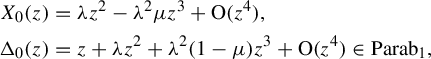
The time-1 map of $X_{0}$
is a generic parabolic germ (Lemma 2.4)
$X_{0}$
is a generic parabolic germ (Lemma 2.4)
 $$ \begin{align*} \Delta_{0}(z):=\Phi_{X_{0}}^{1}(z) =z+\unicode{x3bb} z^{2}+\unicode{x3bb}^{2}(1-\mu)z^{3}+\mathrm{o}(z^{3}) \end{align*} $$
with trivial BÉV modulus. Any germ ![]() with the same
with the same $\mu $
is formally conjugate to
$\mu $
is formally conjugate to $\Delta _{0}$
(whatever
$\Delta _{0}$
(whatever $\unicode{x3bb} $
), which explains the terminology formal model.
$\unicode{x3bb} $
), which explains the terminology formal model.
The sectors and the model $X_{0}$
are tailored in such a way that the orbital region of
$X_{0}$
are tailored in such a way that the orbital region of $\Delta _{0}$
, as seen from the intersection
$\Delta _{0}$
, as seen from the intersection $V^{\cap }$
, is a neighbourhood of
$V^{\cap }$
, is a neighbourhood of $0$
or
$0$
or $\infty $
of size
$\infty $
of size ![]() as
as $\unicode{x3bb} \to 0$
(cf. §4.1). Gaining such a control is essential: eventually the neighbourhood fits within the discs of convergence of the data
$\unicode{x3bb} \to 0$
(cf. §4.1). Gaining such a control is essential: eventually the neighbourhood fits within the discs of convergence of the data ![]() and keeps lying there even after small perturbations.
and keeps lying there even after small perturbations.
Picking $X_{0}$
among all vector fields realizing the trivial pair
$X_{0}$
among all vector fields realizing the trivial pair $({e}^{4\pi ^{2}\mu }\mathrm {Id},\mathrm {Id})$
is arguably canonical since the pullback
$({e}^{4\pi ^{2}\mu }\mathrm {Id},\mathrm {Id})$
is arguably canonical since the pullback $z\mapsto {\unicode{x3bb} z}/({1-z^{2}})$
is very simple and the pair of sectors
$z\mapsto {\unicode{x3bb} z}/({1-z^{2}})$
is very simple and the pair of sectors $(V^{+},V^{-})$
is fairly standard.
$(V^{+},V^{-})$
is fairly standard.
Remark 1.4. For technical reasons, we also need that $\infty $
and
$\infty $
and $0$
be mapped to
$0$
be mapped to $0$
by the pullback. Thereby, the ‘obvious’ choice of a degree-1 pullback, like
$0$
by the pullback. Thereby, the ‘obvious’ choice of a degree-1 pullback, like $z\mapsto {\unicode{x3bb} z}/({1-z})$
, cannot be used to perform the construction presented here. Apart from this restriction, one can use pretty much any other pullback, provided the ‘sectors’ are tailored conveniently.
$z\mapsto {\unicode{x3bb} z}/({1-z})$
, cannot be used to perform the construction presented here. Apart from this restriction, one can use pretty much any other pullback, provided the ‘sectors’ are tailored conveniently.
Example 1.5. We refer to Figure 5. Assume here that $\mu :=0$
so that
$\mu :=0$
so that
 $$ \begin{align*} X_{0}(z) =\frac{\unicode{x3bb} z^{2}}{1+z^{2}}\frac{\partial}{\partial z} \end{align*} $$
has only stationary (double) points at $0$
and
$0$
and $\infty $
, as well as two simple poles at
$\infty $
, as well as two simple poles at $\pm {i}$
with residue
$\pm {i}$
with residue $\pm {\unicode{x3bb} {i}}/{2}$
. These poles spawn the ramification locus of
$\pm {\unicode{x3bb} {i}}/{2}$
. These poles spawn the ramification locus of $\Delta _{0}$
, as can be seen from a direct integration of
$\Delta _{0}$
, as can be seen from a direct integration of $\dot {z}=X_{0}(z)$
at time
$\dot {z}=X_{0}(z)$
at time $1$
with initial value
$1$
with initial value $z_{*}$
:
$z_{*}$
:
 $$ \begin{align*} 1 =\int_{z_{*}}^{\Delta_{0}(z_{*})}\frac{1+z^{2}}{\unicode{x3bb} z^{2}}\,\mathit{d}z, \end{align*} $$
which yields
 $$ \begin{align*} z_{*}\Delta_{0}(z_{*})^{2}-(z_{*}^{2}+\unicode{x3bb} z_{*}-1)\Delta_{0}(z_{*})-z_{*} =0. \end{align*} $$
Hence, $\Delta _{0}$
is algebraic and its ramification points are the four points z for which
$\Delta _{0}$
is algebraic and its ramification points are the four points z for which
 $$ \begin{align*} (z^{2}+\unicode{x3bb} z-1)^{2}+4z^{2} =0. \end{align*} $$
Notice that $\Delta _{0}$
admits a limit at each one of these points z, and
$\Delta _{0}$
admits a limit at each one of these points z, and $\Delta _{0}(z)$
lies within the polar locus
$\Delta _{0}(z)$
lies within the polar locus $\{ \pm {i}\} $
of
$\{ \pm {i}\} $
of $X_{0}$
. Therefore,
$X_{0}$
. Therefore, $\Delta _{0}$
extends as a multivalued function over the domain
$\Delta _{0}$
extends as a multivalued function over the domain $\overline {\mathbb {C}}\backslash \{ z^{2}+\unicode{x3bb} z=1\} $
(which contains
$\overline {\mathbb {C}}\backslash \{ z^{2}+\unicode{x3bb} z=1\} $
(which contains $0$
) with involutive monodromy around any one of the ramification points given by the action of
$0$
) with involutive monodromy around any one of the ramification points given by the action of $\sigma $
, which is moreover sent to a pole of
$\sigma $
, which is moreover sent to a pole of $X_{0}$
by the time-1 map. More details can be found in Lemma 2.7.
$X_{0}$
by the time-1 map. More details can be found in Lemma 2.7.
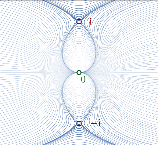
Figure 5 Foliation induced by the real-time flow of $X_{0}$
for
$X_{0}$
for $\mu :=0$
, revealing the double stationary point (green circle) and two simple poles (red squares) (colour online).
$\mu :=0$
, revealing the double stationary point (green circle) and two simple poles (red squares) (colour online).
Remark 1.6. When $\mu \neq 0$
, the mapping
$\mu \neq 0$
, the mapping $\Delta _{0}$
cannot be algebraic (see [Reference ÉcalleÉca75]). It seems safe to conjecture that the only algebraic normal form
$\Delta _{0}$
cannot be algebraic (see [Reference ÉcalleÉca75]). It seems safe to conjecture that the only algebraic normal form $\Delta $
is
$\Delta $
is $\Delta _{0}$
when
$\Delta _{0}$
when $\mu =0$
.
$\mu =0$
.
1.2.2 Link with Écalle canonical synthesis
In [Reference EcalleEca05], J. Écalle revisits the inverse problem by performing the canonical-spherical synthesis using the framework of resurgent functions and alien/mould calculus (for details, see [Reference ÉcalleÉca85]) that he developed in the wake of his original paper [Reference ÉcalleÉca75]. In that setting, the modulus is not built from dynamical considerations, as was first done by G. Birkhoff, himself and S. Voronin (the viewpoint taken here), but as coefficients $(A_{n})_{n\in \mathbb {Z}}$
coming from the associated resurgence equation and carried by the discrete set of singularities of the analytic continuation of the Borel transform of the formal normalization
$(A_{n})_{n\in \mathbb {Z}}$
coming from the associated resurgence equation and carried by the discrete set of singularities of the analytic continuation of the Borel transform of the formal normalization $\Delta \widehat {\sim }\Delta _{0}$
. The link between the pair
$\Delta \widehat {\sim }\Delta _{0}$
. The link between the pair ![]() and the collection
and the collection $(A_{n})_{n}$
is described in [Reference EcalleEca05, §5.1].
$(A_{n})_{n}$
is described in [Reference EcalleEca05, §5.1].
To perform the canonical-spherical synthesis, J. Écalle introduced a (usually large) parameter he called the twist $c>0$
, corresponding here to
$c>0$
, corresponding here to ${1}/{\unicode{x3bb} }$
, and a family of resurgent monomials that served as building blocks for his synthesis. It turns out that the normal forms produced here are very likely the objects obtained by J. Écalle, as witnessed, for instance, by the definition of the Cauchy-like kernel [Reference EcalleEca05, §§5.1 and 10.3], which is pretty much the one involved in the present construction (compare Definition 4.13).
${1}/{\unicode{x3bb} }$
, and a family of resurgent monomials that served as building blocks for his synthesis. It turns out that the normal forms produced here are very likely the objects obtained by J. Écalle, as witnessed, for instance, by the definition of the Cauchy-like kernel [Reference EcalleEca05, §§5.1 and 10.3], which is pretty much the one involved in the present construction (compare Definition 4.13).
Canonical-Spherical Synthesis Conjecture. Given data ![]() and
and $0<\unicode{x3bb} \leq \unicode{x3bb} (\psi )$
, define the twist
$0<\unicode{x3bb} \leq \unicode{x3bb} (\psi )$
, define the twist ![]() . The normal form
. The normal form $\Delta $
given by the Synthesis Theorem is then the parabolic germ coming from Écalle’s canonical-spherical synthesis.
$\Delta $
given by the Synthesis Theorem is then the parabolic germ coming from Écalle’s canonical-spherical synthesis.
If it were true, this would allow us to invoke the effective methods provided by [Reference EcalleEca05] in the present dynamical context. Conversely, let us discuss in which sense the approach given here completes and sheds a dynamical light on Écalle’s synthesis for parabolic germs. To quote J. Écalle (the reader should be aware that he works in the variable ${1}/{z}$
):
${1}/{z}$
):
‘As already pointed out, our twisted monomials have much the same behavior at both poles of the Riemann sphere. The exact correspondence has just been described ${[}\cdots {]}$
using the so-called antipodal involution: in terms of the objects being produced, this means that canonical object synthesis automatically generates two objects: the ‘true’ object, local at
${[}\cdots {]}$
using the so-called antipodal involution: in terms of the objects being produced, this means that canonical object synthesis automatically generates two objects: the ‘true’ object, local at $\infty $
and with exactly the prescribed invariants, and a ‘mirror reflection’, local at 0 and with closely related invariants. Depending on the nature of the
$\infty $
and with exactly the prescribed invariants, and a ‘mirror reflection’, local at 0 and with closely related invariants. Depending on the nature of the ${[}\cdots {]}$
invariants (verification or non-verification of an ‘overlapping condition’), these two objects may or may not link up under analytic continuation on the Riemann sphere.’
${[}\cdots {]}$
invariants (verification or non-verification of an ‘overlapping condition’), these two objects may or may not link up under analytic continuation on the Riemann sphere.’
It could happen that both synthesis processes produce different objects, but what is sure is that the objects built in this paper match very precisely the above expectations and comments. In our setting, the mirror reflection comes from the degree-2 pullback $\Pi :z\mapsto {\unicode{x3bb} z}/({1-z^{2}})$
invariant by the symmetry
$\Pi :z\mapsto {\unicode{x3bb} z}/({1-z^{2}})$
invariant by the symmetry $\sigma $
. The Synthesis Theorem gives quantitative bounds and a uniqueness statement that are not readily available from [Reference EcalleEca05], while the Globalization Theorem simply tells that the normal form is defined and injective on almost all of
$\sigma $
. The Synthesis Theorem gives quantitative bounds and a uniqueness statement that are not readily available from [Reference EcalleEca05], while the Globalization Theorem simply tells that the normal form is defined and injective on almost all of $\mathbb {C}$
. Although it is true that the Taylor series of
$\mathbb {C}$
. Although it is true that the Taylor series of $\Delta $
at
$\Delta $
at $0$
and that of its companion near
$0$
and that of its companion near $\infty $
have a radius of convergence of order
$\infty $
have a radius of convergence of order $1+\mathrm {O}(\sqrt {\unicode{x3bb} })$
, both germs are unconditionally obtained by analytic continuation one from the other, provided of course that
$1+\mathrm {O}(\sqrt {\unicode{x3bb} })$
, both germs are unconditionally obtained by analytic continuation one from the other, provided of course that $0<\unicode{x3bb} \leq \unicode{x3bb} (\psi )$
. In our synthesis, the ‘closely related’ moduli are, in fact, mutually reciprocal.
$0<\unicode{x3bb} \leq \unicode{x3bb} (\psi )$
. In our synthesis, the ‘closely related’ moduli are, in fact, mutually reciprocal.
1.2.3 General parabolic and rationally indifferent germs
Even though in this article, we address in detail only the case of germs in ![]() , our construction can be adapted in a straightforward manner to the space
, our construction can be adapted in a straightforward manner to the space ![]() consisting in those germs in the form
consisting in those germs in the form $\Delta (z)=z+*z^{k+1}+\mathrm {o}(z^{k+1})$
for some
$\Delta (z)=z+*z^{k+1}+\mathrm {o}(z^{k+1})$
for some $k\in \mathbb {Z}_{>0}$
. The inverse problem then regards the realization of collections
$k\in \mathbb {Z}_{>0}$
. The inverse problem then regards the realization of collections ![]() and, in that case, every ingredient must be considered pulled-back by the branched-covering
and, in that case, every ingredient must be considered pulled-back by the branched-covering $z\mapsto z^{k}$
. Namely:
$z\mapsto z^{k}$
. Namely:
-
• the formal model
$X_{0,k}$
is given by the pullback of
$({x^{k+1}}/({1+\mu x^{k}})){\partial }/{\partial x}$
by the mapping
$\Pi _{k}:z\mapsto {\unicode{x3bb} z}/{(1-z^{2k})^{{1}/{k}}}$
, which is invariant by the
$2k$
-periodic homography
$\sigma _{k}:={{e}^{{i}{\pi }/{k}}}{\mathrm {Id}}$
; -
• the normal form is
$({1}/({1+X_{0,k}\cdot F}))X_{0,k}$
with a k-summable
$F\in z\mathbb {C}[[z]] $
; -
• F admits bounded k-sums on infinite sectors
$V_{j}^{\pm }:=\{ z\neq 0:\lvert \arg (\pm z^{k})\rvert <{5\pi }/{8}\} $
, , which are circularly permuted by
$\sigma _{k}$
.


The general case of a rationally indifferent germ ![]() with coprime integers p and q, not conjugate to a rational rotation, can also be recovered from the study we perform here.
with coprime integers p and q, not conjugate to a rational rotation, can also be recovered from the study we perform here.
1.3 Parabolic renormalization
Iteration near a parabolic fixed-point is an important topic in dynamical systems, since complicated phenomena arise once a perturbation is made. Some significant consequences include [Reference Avila and LyubichAL22, Reference Buff and ChéritatBC10, Reference ShishikuraShi98], in which the (near-)parabolic renormalization and its fixed-points play an important role.
The parabolic renormalization map
associates the $\infty $
-component of the invariant of a generic parabolic germ
$\infty $
-component of the invariant of a generic parabolic germ $\Delta $
. It may happen that
$\Delta $
. It may happen that $\mathcal {R}(\Delta )$
is itself generic, in which case,
$\mathcal {R}(\Delta )$
is itself generic, in which case, $\mathcal {R}$
can be iterated. As far as I know, a statement of the kind (while not referring specifically to spherical normal forms) was first communicated privately by R. Schäfke.
$\mathcal {R}$
can be iterated. As far as I know, a statement of the kind (while not referring specifically to spherical normal forms) was first communicated privately by R. Schäfke.
Parabolic Renormalization Corollary. Take an arbitrary ![]() . There exists a bound
. There exists a bound ![]() such that, for all
such that, for all ![]() , there exists a unique spherical normal form
, there exists a unique spherical normal form $\Delta $
satisfying
$\Delta $
satisfying
Again, the bound $\widehat {\unicode{x3bb} }$
can be made explicit, we refer to Corollary 6.3.
$\widehat {\unicode{x3bb} }$
can be made explicit, we refer to Corollary 6.3.
1.4 Real case
If ![]() is real (that is, commutes with the complex conjugation
is real (that is, commutes with the complex conjugation $\overline {\bullet }$
), then
$\overline {\bullet }$
), then $\mu \in \mathbb {R}$
and its modulus
$\mu \in \mathbb {R}$
and its modulus ![]() satisfies the identity:
satisfies the identity:
Real Synthesis Corollary. Take $\mu \in \mathbb {R}$
, a pair
$\mu \in \mathbb {R}$
, a pair ![]() and
and $\unicode{x3bb}>0$
as in the Synthesis Theorem. If, moreover, the identity
$\unicode{x3bb}>0$
as in the Synthesis Theorem. If, moreover, the identity $(\square )$
holds, then the synthesized normal form
$(\square )$
holds, then the synthesized normal form $\Delta $
is real.
$\Delta $
is real.
1.5 Structure of the article and summary of the proofs
One of the main concerns of this paper is to provide as explicit bounds as possible, which explains why so much effort went into technical lemmas. The main tools are basic calculus / complex analysis, and the work is necessary in any case to obtain uniform bounds with respect to $\unicode{x3bb} $
.
$\unicode{x3bb} $
.
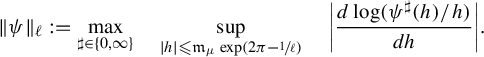
All the constructions will take place within the space of pairs $f=(f^{+},f^{-})$
with 1-flat difference in
$f=(f^{+},f^{-})$
with 1-flat difference in $V^{\cap }$
and bounded 1-type, both at
$V^{\cap }$
and bounded 1-type, both at $0$
and
$0$
and $\infty $
, as discussed at the beginning of the introduction:
$\infty $
, as discussed at the beginning of the introduction:
 $$ \begin{align*} \mathcal{S} :=\big\{ f\in\mathcal{S}(V^{+})\times\mathcal{S}(V^{-}):\limsup_{z^{\pm1}\to0}|z|^{\pm1}\ln|f^{-}(z)-f^{+}(z)|\leq-5\text{ for }z\in V^{\cap}\big\} , \end{align*} $$
where

is equipped with the canonical product Banach norm. We denote by $\mathcal {B}$
its unit ball.
$\mathcal {B}$
its unit ball.
Remark 1.7. Actually, the uniform bound $-5$
on the
$-5$
on the $1$
-type of
$1$
-type of $f^{-}-f^{+}$
can be sharpened as
$f^{-}-f^{+}$
can be sharpened as $-{5}/{\unicode{x3bb} }$
(see equation (3.5)), that is, the difference becomes increasingly flatter as
$-{5}/{\unicode{x3bb} }$
(see equation (3.5)), that is, the difference becomes increasingly flatter as $\unicode{x3bb} $
tends to
$\unicode{x3bb} $
tends to $0$
, although we do not need that fact.
$0$
, although we do not need that fact.
-
(1) In §2, we give some basic material about vector fields and their time-1 maps, focusing more particularly on the local dynamics near their poles and zeroes, and how they stitch together to organize the global dynamics of the model
$X_{0}$
. This will allow us to conjugate to the model
$$ \begin{align*} X_{f}^{\pm} :=\frac{1}{1+X_{0}\cdot f^{\pm}}X_{0} \end{align*} $$
$X_{0}$
over the better part of
$V^{\pm }$
(effective bounds are described in §5.2). This sectorial mapping takes the form
$\Phi _{X_{0}}^{f^{\pm }}$
given by the flow of
$X_{0}$
at time
$f^{\pm }$
. The dynamics of the formal model
$\Delta _{0}$
, studied in §2.3, is then pulled-back by
$\Psi ^{\pm }$
to give sectorial counterparts for the time-1 map of
$X_{f}^{\pm }$
.
-
(2) Coupled to the Ramis–Sibuya theorem, the above preliminary part allows one to reduce the problem of finding a parabolic germ
$\Delta $
with prescribed modulus to that of finding
$(f^{+},f^{-})\in \mathcal {S}$
satisfying some (nonlinear) Cousin problem
$(\star )$
below; see Proposition 3.3 in §3. -
(3) We can then tackle the main result (§4). We begin with fixing a formal class
$\mu \in \mathbb {C}$
in . Then, must be tangent to the linear map
${e}^{4\pi ^{2}\mu }\mathrm {Id}$
. Being given with holomorphic near
$\sharp \in \{ 0,\infty \} $
, we must find
$f^{\pm }$
on
$V^{\pm }$
such that (⋆)where are the two components of
$V^{\cap }$
, and
$H_{f}^{+}$
is a primitive first-integral of the sectorial time-1 map
$\Delta ^{+}$
of
$X_{f}^{+}$
(in other words,
$H_{f}^{+}$
provides preferred orbital coordinates over the sector
$V^{+}$
). Condition
$(\star )$
implies that
$\Delta ^{+}$
coincides with
$\Delta ^{-}$
in
$V^{\cap }$
and thus is the restriction to
$V^{+}$
of a single .
The nonlinear Cousin problem
$(\star )$
is solved using a fixed-point method involving a classical Cauchy–Heine integral transform. This technique was already employed in [Reference Schäfke and TeyssierST15] (and [Reference Rousseau and TeyssierRT21]) to build normal forms for convergent saddle-node foliations in the complex plane (and their unfoldings). More precisely, we build a map (Proposition 4.11): such that
$\Lambda (f)^{-}-\Lambda (f)^{+}=\varphi \circ H_{f}^{+}$
. Therefore, if and only if condition
$(\star )$
holds. We prove (Proposition 4.14) that eventually stabilizes the unit ball
$\mathcal {B}\subset \mathcal {S}$
. The smaller
$\unicode{x3bb} $
, the more contracting , so that eventually a unique fixed-point of exists in that ball (Corollary 4.15).
-
(4) In §5.1, as is discussed above, we establish the Globalization Theorem making use of the involution
$\sigma $
and the property that for the fixed-point f of , we have Prior to that, we describe the dynamical properties of
$$ \begin{align*} f^{\pm}\circ\sigma =-f^{\mp}. \end{align*} $$
$\Delta $
in §5.3 using a priori bounds on the flow of
$X^{\pm }$
.
-
(5) The fixed-points of the parabolic renormalization are also obtained as a holomorphic fixed-point in §6.1. Let
$\text {Synth}_{\unicode{x3bb} }:\psi \mapsto \Delta $
be the synthesis map built previously and consider for given , the iterations
$\Delta _{0}:=\mathrm {Id}$
and . It so happens that
$\text {Synth}_{\unicode{x3bb} }$
cannot shrink too much the radius of convergence of
$\Delta _{n}$
, which always remains above
${3}/{16}$
. By taking
$\unicode{x3bb} $
smaller, we prove next that
$\text {Synth}_{\unicode{x3bb} }$
is a contracting self-map of some closed ball of the Banach space . -
(6) The real setting is explored in §6.2 (Real Synthesis Corollary). It merely consists in checking that every step leading to the fixed-point of
preserves realness, which is straightforward.


1.6 Notation
-
•
$\dot {z}={\mathit {d}z}/{\mathit {d}t}$
stands for differentiation with respect to the variable
$t\in \mathbb {C}$
. -
• For a topological space
$\mathcal {M}$
and a point
$p\in \mathcal {M}$
, we use
$(\mathcal {M},p)$
to stand for a (sufficiently small) neighbourhood of p in
$\mathcal {M}$
. -
• The set
$\overline {U}$
is the topological closure of
$U\subset \mathcal {M}$
. -
• We use the notation
$\mathbb {D}$
for the standard open unit disk in
$\mathbb {C}$
. -
•
$\overline {\mathbb {C}}$
stands for the compactification of the complex line
$\mathbb {C}$
as the Riemann sphere. -
• The nth iterate of a diffeomorphism
$\Delta $
is written
$\Delta ^{\circ n}$
for
$n\in \mathbb {Z}$
. -
•
$\Phi _{X}^{t}$
designates the flow at time t of the vector field X. -
• If
$\Psi :U\to V$
is locally biholomorphic, we recall its action by conjugacy (change of coordinate) on diffeomorphisms: on vector fields:
$$ \begin{align*} \Psi^{*}\Delta :=\Psi^{\circ-1}\circ\Delta\circ\Psi, \end{align*} $$
If
$$ \begin{align*} \Psi^{*}X :=\mathrm{D}\Psi^{\circ-1}(X\circ\Psi). \end{align*} $$
$\Delta $
is the time-1 map of X, then
$\Psi ^{*}\Delta $
is the time-1 map of
$\Psi ^{*}X$
.


2 Sectorial normalization
We recall that the functional space $\mathcal {S}$
is defined in §1.5 above. The main purpose of this section is to investigate, in some detail, the dynamics of
$\mathcal {S}$
is defined in §1.5 above. The main purpose of this section is to investigate, in some detail, the dynamics of
which we deduce from two ingredients:
-
• the dynamics of the rational vector field
(2.1)studied in §2.3;
$$ \begin{align} X_{0}(z):= \frac{1-z^{2}}{1+z^{2}}\times\frac{\unicode{x3bb} z^{2}}{1+\unicode{x3bb}\mu z-z^{2}}\frac{\partial}{\partial z} \end{align} $$
-
• the sectorial normalization between
$X^{\pm }$
and
$X_{0}$
obtained in §2.4, that is, the existence of biholomorphisms on
$V^{\pm }\backslash \{ \text {small neighbourhhood of the poles}\} $
conjugating the dynamics of both vector fields.


The dynamics of a meromorphic vector field X on some domain U is organized by its singular locus, which splits between the stationary points and the poles
 $$ \begin{align*} \text{Zero}(X) & :=\{ z\in U:X(z)=0\}, \\ \mathrm{Pole}(X) & :=\{ z\in U:X(z)=\infty\}. \end{align*} $$
Since $f^{\pm }$
is holomorphic on
$f^{\pm }$
is holomorphic on $V^{\pm }$
, we can never have
$V^{\pm }$
, we can never have ${1}/({1+X_{0}\cdot f^{\pm }})=0$
except at the poles of
${1}/({1+X_{0}\cdot f^{\pm }})=0$
except at the poles of $X_{0}$
, and hence,
$X_{0}$
, and hence,
 $$ \begin{align*} \text{Zero}(X^{+})\cup\,\text{Zero}(X^{-}) =\text{Zero}(X_{0}). \end{align*} $$
It is also true that $z\in \mathrm {Pole}(X^{\pm })$
if and only if:
$z\in \mathrm {Pole}(X^{\pm })$
if and only if:
-
•
$z\in \mathrm {Pole}(X_{0})$
and
$(f^{\pm })'(z)=0$
; -
• or
$z\notin \mathrm {Pole}(X_{0})$
and
$1+(X_{0}\cdot f^{\pm })(z)=0$
.


We begin with fixing some notation and recall the important Lie formula regarding holomorphic vector fields X, then proceed to a short description of the local behaviour of the trajectories near singularities and finally explain how the global dynamics of rational X is woven from these local parts.
2.1 Basic vector fields material
2.1.1 Flow and time-1 map
Let $U\subset \overline {\mathbb {C}}$
be a domain and
$U\subset \overline {\mathbb {C}}$
be a domain and $X=R({\partial }/{\partial z})$
be a holomorphic vector field on U (that is, R is a holomorphic function on U). For any
$X=R({\partial }/{\partial z})$
be a holomorphic vector field on U (that is, R is a holomorphic function on U). For any $z_{*}\in U$
, the differential system
$z_{*}\in U$
, the differential system $\dot {z}=X(z)$
has a unique local solution
$\dot {z}=X(z)$
has a unique local solution $t\in (\mathbb {C},0)\mapsto z(t)$
with
$t\in (\mathbb {C},0)\mapsto z(t)$
with $z(0)=z_{*}$
, giving rise to a germ of a holomorphic mapping
$z(0)=z_{*}$
, giving rise to a germ of a holomorphic mapping
(to be more correct, the neighbourhood ![]() depends on
depends on $z_{*}$
, but its size is locally uniform). The flow of X is the maximal multivalued analytic continuation of
$z_{*}$
, but its size is locally uniform). The flow of X is the maximal multivalued analytic continuation of $\Phi _{X}^{}$
. It is probably best understood as the reciprocal of the time function
$\Phi _{X}^{}$
. It is probably best understood as the reciprocal of the time function
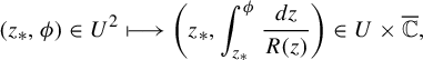 $$ \begin{align} (z_{*},\phi)\in U^{2} \longmapsto\bigg(z_{*},\int_{z_{*}}^{\phi}\frac{\mathit{d}z}{R(z)}\bigg)\in U\times\overline{\mathbb{C}}, \end{align} $$
obtained by rewriting $\dot {z}=X(z)$
as
$\dot {z}=X(z)$
as $\mathit {d}t=\mathit {d}z/{R(z)}$
and integrating the time form
$\mathit {d}t=\mathit {d}z/{R(z)}$
and integrating the time form
 $$ \begin{align} \tau_{X} :=\frac{\mathit{d}z}{R}. \end{align} $$
The analytic continuation of the time function is explicit, at least when R is rational.
Definition 2.1. We call $\Delta :z\mapsto \Phi _{X}^{1}(z)$
the time-1 map of X. As a multivalued mapping over U, for any path
$\Delta :z\mapsto \Phi _{X}^{1}(z)$
the time-1 map of X. As a multivalued mapping over U, for any path $\gamma :[0,1]\to U$
satisfying
$\gamma :[0,1]\to U$
satisfying
 $$ \begin{align*} 1 =\int_{\gamma}\tau_{X}, \end{align*} $$
a determination of $\Delta $
satisfies the identity
$\Delta $
satisfies the identity
 $$ \begin{align*} \Delta(\gamma(0)) =\gamma(1), \end{align*} $$
with the special case $\Delta (z)=z$
if
$\Delta (z)=z$
if $X(z)=0$
.
$X(z)=0$
.
Remark 2.2. For $t\in \mathbb {C}^{\times }$
, the time-t map
$t\in \mathbb {C}^{\times }$
, the time-t map $\Phi _{X}^{t}$
is obtained as the time-1 map of
$\Phi _{X}^{t}$
is obtained as the time-1 map of $({1}/{t})X$
.
$({1}/{t})X$
.
2.1.2 Lie’s formula
One also encounters the notation $\exp (tX)$
to stand for
$\exp (tX)$
to stand for $\Phi _{X}^{t}$
. This can be understood in the light of Lie’s formula relating the action of the operator
$\Phi _{X}^{t}$
. This can be understood in the light of Lie’s formula relating the action of the operator $\exp (tX)$
and of the flow mapping. Pick a function
$\exp (tX)$
and of the flow mapping. Pick a function ![]() and some
and some $z\in U$
. For any
$z\in U$
. For any ![]() , one has
, one has
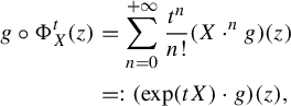 $$ \begin{align} g\circ\Phi_{X}^{t}(z) & =\sum_{n=0}^{+\infty}\frac{t^{n}}{n!}(X\cdot^{n}g)(z)\\ & =:(\exp(tX)\cdot g)(z),\nonumber \end{align} $$
where the iterated Lie’s derivative is defined by
 $$ \begin{align*} X\cdot^{n}g :=\underset{n\text{ times}}{\underbrace{X\cdot X\cdot(\cdots)\cdot X\cdot}}g. \end{align*} $$
2.1.3 Long-time behaviour
In this paper, we only use the real-time flow, that is, for $t\in (\mathbb {R},0)$
, and designate by
$t\in (\mathbb {R},0)$
, and designate by $t_{\max }(z_{*})\in ]0,+\infty ]$
the maximal time of existence of the forward trajectory
$t_{\max }(z_{*})\in ]0,+\infty ]$
the maximal time of existence of the forward trajectory $t\in [0,t_{\max }(z_{*})[\mapsto \Phi _{X}^{t}(z_{*})$
. Without going into too much detail, a consequence of the Bendixson–Poincaré theorem and of Cauchy’s formula applied to equation (2.2) is the following classification of asymptotic behaviour for the real flow of a meromorphic vector field X on some domain U. Starting from
$t\in [0,t_{\max }(z_{*})[\mapsto \Phi _{X}^{t}(z_{*})$
. Without going into too much detail, a consequence of the Bendixson–Poincaré theorem and of Cauchy’s formula applied to equation (2.2) is the following classification of asymptotic behaviour for the real flow of a meromorphic vector field X on some domain U. Starting from $z_{*}\notin \mathrm {Pole}(X)$
, the forward trajectory
$z_{*}\notin \mathrm {Pole}(X)$
, the forward trajectory $t\geq 0\mapsto z(t)$
matches one of the mutually exclusive outcomes:
$t\geq 0\mapsto z(t)$
matches one of the mutually exclusive outcomes:
-
(1) either
$t_{\max }(z_{*})=\infty $
, exactly in the following situations:centre case: z is periodic (non-constant), in which case, neighbouring trajectories also are (with same period) and at least one stationary point of X of centre type is enclosed by the trajectory;
equilibrium case:
$\lim _{t\to +\infty }z(t)\in \text {Zero}(X)$
; -
(2) or
$t_{\max }(z_{*})<\infty $
, exactly in the following situations:escape case:
$\lim _{t\to t_{\max }(z_{*})}z(t)\in \partial U$
;separation case:
$\lim _{t\to t_{\max }(z_{*})}z(t)\in \mathrm {Pole}(X)$
.


2.2 Local behaviour near singularities
2.2.1 Dynamics near a simple zero
Let $p\in \overline {\mathbb {C}}$
be a simple stationary point of a meromorphic vector field
$p\in \overline {\mathbb {C}}$
be a simple stationary point of a meromorphic vector field $X=R({\partial }/{\partial z})$
, and denote by
$X=R({\partial }/{\partial z})$
, and denote by $\alpha \neq 0$
the derivative of R at this point. One can find a conformal coordinate
$\alpha \neq 0$
the derivative of R at this point. One can find a conformal coordinate $z=\Psi (w)$
near p such that X takes the form
$z=\Psi (w)$
near p such that X takes the form
A direct integration describes the local behaviour of the dynamics of the linear vector field around a simple zero:
 $$ \begin{align*} \Phi_{W}^{t}(w) =w{e}^{\alpha t}. \end{align*} $$
In particular, the time-1 map of X is linearizable near its fixed-point p, which can be of three types:
-
• attractive (
$\mathrm {Re}(\alpha )<0$
) or repulsive (
$\mathrm {Re}(\alpha )>0$
) in the equilibrium case; then there exists a domain
$U:=(\overline {\mathbb {C}},p)$
such that any trajectory crossing
$\partial U$
converges asymptotically to p in forward or backward time (a basin of attraction/repulsion); -
• but it can also be a centre case (
$\mathrm {Re}(\alpha )=0$
).


Example 2.3. When $\mu \neq 0$
, the formal model
$\mu \neq 0$
, the formal model $X_{0}$
admits a simple stationary point at
$X_{0}$
admits a simple stationary point at $\pm 1$
with linear part
$\pm 1$
with linear part $\alpha =-{1}/{\mu }$
.
$\alpha =-{1}/{\mu }$
.
2.2.2 Dynamics near a double zero
Take now a double zero of X which, for the sake of convenience, we locate at $0$
, and define the constants
$0$
, and define the constants $a\neq 0$
and b by
$a\neq 0$
and b by
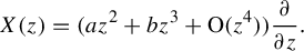 $$ \begin{align*} X(z) =(az^{2}+bz^{3}+\mathrm{O}(z^{4}))\frac{\partial}{\partial z}. \end{align*} $$
Lemma 2.4. For all $a\in \mathbb {C}^{\times }$
and
$a\in \mathbb {C}^{\times }$
and $b\in \mathbb {C}$
, we have
$b\in \mathbb {C}$
, we have ![]() . More precisely, the
. More precisely, the $3$
-jet of the mapping at
$3$
-jet of the mapping at $0$
is given by
$0$
is given by
 $$ \begin{align*} \Phi_{X}^{1}(z) =z+az^{2}+(a^{2}+b)z^{3}+\mathrm{O}(z^{4}). \end{align*} $$
This germ is linearly conjugate to $w\mapsto w+w^{2}+(1+{b}/{a^{2}})w^{3}+\mathrm {o}(w^{3})$
through the transform
$w\mapsto w+w^{2}+(1+{b}/{a^{2}})w^{3}+\mathrm {o}(w^{3})$
through the transform $w:=az$
, and hence the formal invariant of
$w:=az$
, and hence the formal invariant of $\Phi _{X}^{1}$
is
$\Phi _{X}^{1}$
is $-{b}/{a^{2}}$
.
$-{b}/{a^{2}}$
.
Proof. Using the Lie formula, we obtain
 $$ \begin{align*} \Phi_{X}^{1}(z) =z+(az^{2}+bz^{3})+a^{2}z^{3}+\mathrm{O}(z^{4}). \end{align*} $$
The rest is straightforward algebra, but for the fact that the formal invariant of $w\mapsto w+w^{2}+cw^{3}+\mathrm {O}(w^{4})$
is
$w\mapsto w+w^{2}+cw^{3}+\mathrm {O}(w^{4})$
is $1-c$
.
$1-c$
.
Example 2.5. In the case of $X_{0}$
, we have
$X_{0}$
, we have
with formal invariant $\mu $
independently on
$\mu $
independently on $\unicode{x3bb} $
.
$\unicode{x3bb} $
.
Remark 2.6. There exists a domain $U:=(\overline {\mathbb {C}},p)$
such that any trajectory crossing
$U:=(\overline {\mathbb {C}},p)$
such that any trajectory crossing $\partial U$
converges asymptotically to p in forward- or backward-time (a parabolic basin).
$\partial U$
converges asymptotically to p in forward- or backward-time (a parabolic basin).
2.2.3 Dynamics near a simple pole (separation case)
Consider here the case where $X(p)=\infty $
is a simple pole. One can find a conformal coordinate
$X(p)=\infty $
is a simple pole. One can find a conformal coordinate $z=\Psi (w)$
near p such that X takes the form
$z=\Psi (w)$
near p such that X takes the form
A direct integration describes the local behaviour of the dynamics of the linear vector field around a simple pole.
Lemma 2.7. Let $W:=({1}/{w}){\partial }/{\partial w}$
. We refer to Figure 6 for an illustration of the statements to come.
$W:=({1}/{w}){\partial }/{\partial w}$
. We refer to Figure 6 for an illustration of the statements to come.
-
(1) The foliation induced by W has a saddle-point at
$0$
with stable manifold
${i}\mathbb {R}$
and unstable manifold
$\mathbb {R}$
.Figure 6 Saddle dynamics near a simple pole of a vector field W and induced slicing dynamics of its time-1 map
$\Delta $
. The latter is holomorphic on the complement of the arc
$\gamma $
, included in the stable manifold and whose endpoints are sent to the pole in time
$1$
(colour online). -
(2) The time-1 map of W is defined and holomorphic on
$\mathbb {C}\backslash \gamma $
with
$\gamma :={i}\sqrt {2}[-1,1]$
, where it evaluates to
$$ \begin{align*} \Phi_{W}^{1}(w) =\pm\sqrt{2+w^{2}}. \end{align*} $$
-
(3) The analytic continuation of the above map as a multivalued function can be realized over
$\mathbb {C}\backslash \{ \pm {i}\sqrt {2}\} $
with monodromy .


Example 2.8. The vector field $X_{0}$
admits two symmetric simple poles
$X_{0}$
admits two symmetric simple poles $\pm {i}$
, fixed by
$\pm {i}$
, fixed by $\sigma $
, as well as two additional simple poles
$\sigma $
, as well as two additional simple poles
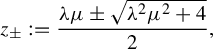 $$ \begin{align*} z_{\pm} :=\frac{\unicode{x3bb}\mu\pm\sqrt{\unicode{x3bb}^{2}\mu^{2}+4}}{2}, \end{align*} $$
swapped by $\sigma $
, provided
$\sigma $
, provided $\mu \neq \pm ({2{i}}/{\unicode{x3bb} })$
(otherwise, it is a double pole
$\mu \neq \pm ({2{i}}/{\unicode{x3bb} })$
(otherwise, it is a double pole $z_{+}=z_{-}=\mu \in {i}\mathbb {R}$
) and
$z_{+}=z_{-}=\mu \in {i}\mathbb {R}$
) and $\mu \neq 0$
(else the pole
$\mu \neq 0$
(else the pole $\pm 1$
cancels out the zero of
$\pm 1$
cancels out the zero of $X_{0}$
located at
$X_{0}$
located at $\pm 1$
).
$\pm 1$
).
Near $\pm {i}$
, the vector field
$\pm {i}$
, the vector field $X_{0}$
is conjugate to
$X_{0}$
is conjugate to $\Phi _{W}^{1}$
and this conjugacy sends
$\Phi _{W}^{1}$
and this conjugacy sends $\sigma $
to the involution
$\sigma $
to the involution $w\mapsto -w$
, so that the monodromy of
$w\mapsto -w$
, so that the monodromy of $\Delta _{0}$
around the ramification points attached to
$\Delta _{0}$
around the ramification points attached to $\pm {i}$
is
$\pm {i}$
is $\sigma $
(the ramification is induced by the change of variable
$\sigma $
(the ramification is induced by the change of variable $\Pi $
). The corresponding local involution near
$\Pi $
). The corresponding local involution near $z_{\pm }$
has a different nature and comes from the involution
$z_{\pm }$
has a different nature and comes from the involution $\nu \neq \mathrm {Id}$
of the usual formal model
$\nu \neq \mathrm {Id}$
of the usual formal model $({x^{2}}/({1+\mu x})){\partial }/{\partial x}$
near the pole
$({x^{2}}/({1+\mu x})){\partial }/{\partial x}$
near the pole $-{1}/{\mu }$
, which solves
$-{1}/{\mu }$
, which solves
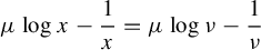 $$ \begin{align*} \mu\log x-\frac{1}{x} =\mu\log\nu-\frac{1}{\nu} \end{align*} $$
(observe indeed that $t\mapsto \mu \log t-{1}/{t}$
has a critical point at
$t\mapsto \mu \log t-{1}/{t}$
has a critical point at $-{1}/{\mu }$
).
$-{1}/{\mu }$
).
Remark 2.9. The case of a kth-order pole $({1}/{w^{k}}){\partial }/{\partial w}$
is similar, with time-1 map
$({1}/{w^{k}}){\partial }/{\partial w}$
is similar, with time-1 map $\Phi _{W}^{1}(w)=(k+1+w^{k+1})^{{1}/({k+1})}$
, giving rise to
$\Phi _{W}^{1}(w)=(k+1+w^{k+1})^{{1}/({k+1})}$
, giving rise to $k+1$
ramification points and
$k+1$
ramification points and $k+1$
determinations of the time-1 map. The integer k is a topological invariant.
$k+1$
determinations of the time-1 map. The integer k is a topological invariant.
2.3 Global dynamics of the formal model
We explain why/how we choose the formal model $X_{0}$
and the sector
$X_{0}$
and the sector $V^{\pm }$
in §4.1. For now, let us present the global features of the dynamics of
$V^{\pm }$
in §4.1. For now, let us present the global features of the dynamics of $X_{0}$
on
$X_{0}$
on $\overline {\mathbb {C}}$
for fixed
$\overline {\mathbb {C}}$
for fixed $\unicode{x3bb}>0$
and
$\unicode{x3bb}>0$
and $\mu \in \mathbb {C}$
. We explain how the local dynamics near the singular set of X we described above stitch together by studying the real-analytic foliation of the sphere
$\mu \in \mathbb {C}$
. We explain how the local dynamics near the singular set of X we described above stitch together by studying the real-analytic foliation of the sphere $\overline {\mathbb {C}}$
induced by the real-time flow (Figure 7).
$\overline {\mathbb {C}}$
induced by the real-time flow (Figure 7).
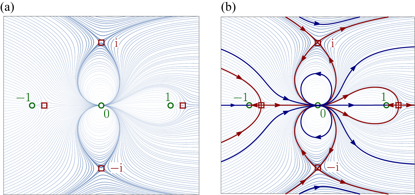
Figure 7 (a) Foliation induced by the real-time flow of $X_{0}$
for
$X_{0}$
for $\unicode{x3bb} :=\tfrac 12$
and
$\unicode{x3bb} :=\tfrac 12$
and $\mu :=\tfrac 12$
, revealing the three stationary points (green circles) and four poles (red squares). (b) The spinal graph (blue, connecting zeroes) and separatrix graph (red, connecting poles to zeroes) (colour online).
$\mu :=\tfrac 12$
, revealing the three stationary points (green circles) and four poles (red squares). (b) The spinal graph (blue, connecting zeroes) and separatrix graph (red, connecting poles to zeroes) (colour online).
Remark 2.10.
-
(1) Whether
$\mu =0$
or not leads to different dynamics, since the simpler
$X_{0}(z)=({\unicode{x3bb} z^{2}}/({1+z^{2}})){\partial }/{\partial z}$
has less poles and zeroes. The dynamics of this particular vector field has been studied in Example 1.5, so we allow ourselves to assume that
$\mu \neq 0$
whenever it leads to a more straightforward exposition. -
(2) To avoid other zero/pole cancellations, we must, in addition, suppose that
$\mu \neq \pm ({2{i}}/{\unicode{x3bb} })$
(the latter is ensured whenever
$\unicode{x3bb} <{1}/{2|\mu |}$
). Under these assumptions, the rational vector field has three stationary points located at
$0$
(double) and
$\pm 1$
(simple), as well as four simple poles located at
$z_{\pm }:=({\unicode{x3bb} \mu \pm \sqrt {\unicode{x3bb} ^{2}\mu ^{2}+4}})/{2}$
and
$\pm {i}$
.


2.3.1 Spinal graph
After the pioneering work of S. Smale et al starting at the beginning of the 1980s to study general numerical Newton-like schemes for solving polynomial equations [Reference SmaleSma81, Reference Shub, Tischler and WilliamsSTW88], the foliations induced by holomorphic polynomial vector fields X have been thoroughly studied in the generic case by Douady, Estrada and Sentenac in an unpublished manuscript [Reference Douady, Estrada and SentenacDES05]. Then, Branner and Dias [Reference Branner and DiasBD10] completed the task for every polynomial vector field and, in his thesis, J. Tomasini studied some rational vector fields. All these considerations result in the following statement: the topological class of X (up to orientation-preserving homeomorphism) is completely classified by its combinatorial dynamics. Roughly speaking, it is encoded as the spinal graph of X, the way poles and stationary points of the vector field are connected by the closure of maximal trajectories.
Lemma 2.11. Let X be a rational vector field. The separatrix graph $\mathrm {Sep}(X)$
of X is the closure of the union of all stable and unstable manifolds passing through the poles of X. Then,
$\mathrm {Sep}(X)$
of X is the closure of the union of all stable and unstable manifolds passing through the poles of X. Then, $\overline {\mathbb {C}}\backslash \mathrm {Sep}(X_{})$
consists in finitely many X-invariant connected components. Any two trajectories in the same component are:
$\overline {\mathbb {C}}\backslash \mathrm {Sep}(X_{})$
consists in finitely many X-invariant connected components. Any two trajectories in the same component are:
-
• either both periodic with same period;
-
• or they link the same pair of stationary points
$q\to p$
of X.

Proof. Assume that $t\mapsto z(t)$
is a periodic trajectory. Cauchy’s formula indicates that nearby trajectories are also periodic with the same period. A straightforward connectedness argument allows us to conclude that every other trajectory in the component is periodic with the same period.
$t\mapsto z(t)$
is a periodic trajectory. Cauchy’s formula indicates that nearby trajectories are also periodic with the same period. A straightforward connectedness argument allows us to conclude that every other trajectory in the component is periodic with the same period.
Assume now that $t\mapsto z(t)$
is neither a centre nor a separatrix. Then, z goes towards some
$t\mapsto z(t)$
is neither a centre nor a separatrix. Then, z goes towards some $p\in \text {Zero}(X)$
in forward time, say, and then there exists a domain
$p\in \text {Zero}(X)$
in forward time, say, and then there exists a domain $U_{p}\ni p$
(the basin of attraction of an attractive fixed-point or a parabolic basin for a multiple zero) such that any trajectory landing at p eventually hits
$U_{p}\ni p$
(the basin of attraction of an attractive fixed-point or a parabolic basin for a multiple zero) such that any trajectory landing at p eventually hits $\partial U_{p}$
and vice versa. Hence, z links
$\partial U_{p}$
and vice versa. Hence, z links $\partial U_{q}$
to
$\partial U_{q}$
to $\partial U_{p}$
in finite time, and the flow-box theorem asserts this remains the case for neighbouring trajectories. Again, a direct connectedness argument brings the conclusion.
$\partial U_{p}$
in finite time, and the flow-box theorem asserts this remains the case for neighbouring trajectories. Again, a direct connectedness argument brings the conclusion.
Definition 2.12. We define the spinal graph $\mathrm {Spine}(X)$
as the oriented graph with vertices
$\mathrm {Spine}(X)$
as the oriented graph with vertices $\text {Zero}(X)$
and ordered edges corresponding to a trajectory of X linking those vertices
$\text {Zero}(X)$
and ordered edges corresponding to a trajectory of X linking those vertices $q\to p$
, one per component of
$q\to p$
, one per component of $\overline {\mathbb {C}}\backslash \mathrm {Sep}(X_{})$
. Isolated vertices correspond to centre stationary points.
$\overline {\mathbb {C}}\backslash \mathrm {Sep}(X_{})$
. Isolated vertices correspond to centre stationary points.
Remark 2.13. Both graphs $\mathrm {Spine}(X)$
and
$\mathrm {Spine}(X)$
and $\mathrm {Sep}(X)$
come with a canonical, non-ambiguous geometric realization with edges as integral curves of X. For that reason, we identify the combinatorial data and its canonical geometric realization as a subset of
$\mathrm {Sep}(X)$
come with a canonical, non-ambiguous geometric realization with edges as integral curves of X. For that reason, we identify the combinatorial data and its canonical geometric realization as a subset of $\overline {\mathbb {C}}$
.
$\overline {\mathbb {C}}$
.
We can equip both graphs with an oriented length, by integrating the time form equation (2.3) along injective subpaths $\gamma $
:
$\gamma $
:
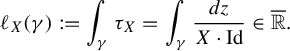 $$ \begin{align} \ell_{X}(\gamma) :=\int_{\gamma}\tau_{X}=\int_{\gamma}\frac{\mathit{d}z}{X\cdot\mathrm{Id}}\in\overline{\mathbb{R}}. \end{align} $$
We omit the proof of the next lemma.
Lemma 2.14. If $\mu \neq 0$
and
$\mu \neq 0$
and $\mu \neq \pm {2{i}}/{\unicode{x3bb} }$
, the graph
$\mu \neq \pm {2{i}}/{\unicode{x3bb} }$
, the graph $\mathrm {Spine}(X_{0})$
belongs to the following list, according to the sign of
$\mathrm {Spine}(X_{0})$
belongs to the following list, according to the sign of $\mathrm {Re}(\mu )$
. A centre bifurcation occurs when
$\mathrm {Re}(\mu )$
. A centre bifurcation occurs when $\mathrm {Re}(\mu )=0$
. In Figure 8, the separatrix graph is represented in red while the spinal graph is coloured blue.
$\mathrm {Re}(\mu )=0$
. In Figure 8, the separatrix graph is represented in red while the spinal graph is coloured blue.
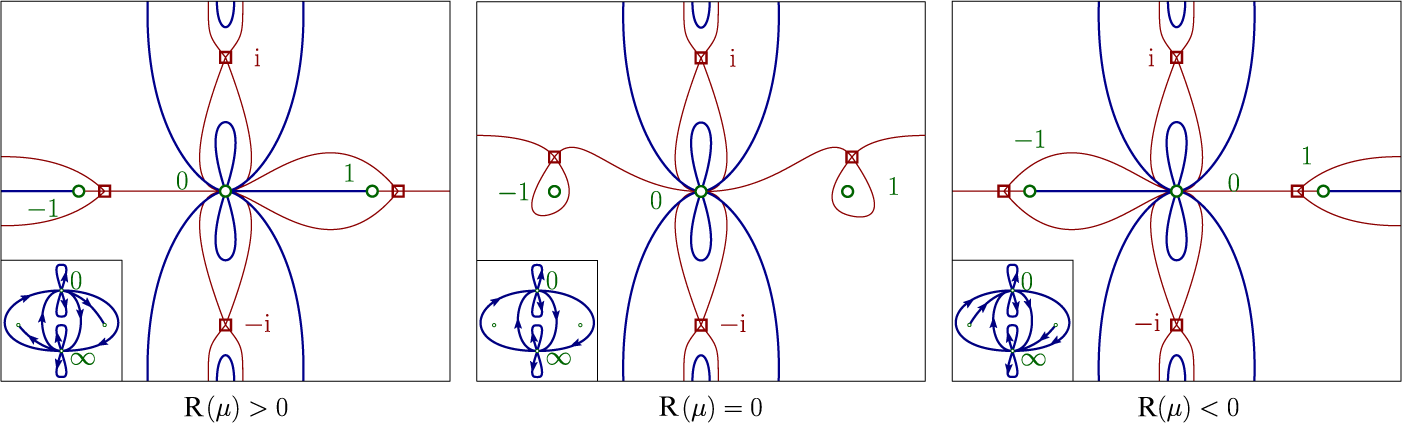
Figure 8 The three distinct spinal and separatrix graphs that can arise for X (the bottom-left boxes represent the combinatorial class of the corresponding spinal graph) (colour online).
2.3.2 Dynamics of the time-1 map
$\Delta _{0}$

From the description of the qualitative dynamics of time-1 maps of rational vector fields, we work out more quantitative specifics for the model $X_{0}$
.
$X_{0}$
.
Lemma 2.15. Let X be a rational vector field and $\Delta $
be its time-1 map. Then,
$\Delta $
be its time-1 map. Then, $\Delta $
is a multivalued map over
$\Delta $
is a multivalued map over $\overline {\mathbb {C}}$
with branch points
$\overline {\mathbb {C}}$
with branch points $z_{*}\in \mathrm {Sep}(X)$
at time-
$z_{*}\in \mathrm {Sep}(X)$
at time- $1$
from an element of
$1$
from an element of $\mathrm {Pole}(X)$
, by which we mean that there exists a subpath
$\mathrm {Pole}(X)$
, by which we mean that there exists a subpath $\gamma \subset \mathrm {Sep}(X)$
with
$\gamma \subset \mathrm {Sep}(X)$
with $\gamma (0)=z_{*}$
,
$\gamma (0)=z_{*}$
, $\gamma (1)\in \mathrm {Pole}(X)$
and
$\gamma (1)\in \mathrm {Pole}(X)$
and $\ell _{X}(\gamma )=1$
as in equation (2.5). A pole of order k gives rise to
$\ell _{X}(\gamma )=1$
as in equation (2.5). A pole of order k gives rise to $k+1$
local determinations.
$k+1$
local determinations.
Proof. For $\Delta $
to be locally holomorphic at
$\Delta $
to be locally holomorphic at $z\in U$
, there must exist a path
$z\in U$
, there must exist a path $\tau :[0,1]\longrightarrow \mathbb {C}$
with
$\tau :[0,1]\longrightarrow \mathbb {C}$
with $\tau (0)=0$
and
$\tau (0)=0$
and $\tau (1)=1$
, on a neighbourhood of whose image the germ
$\tau (1)=1$
, on a neighbourhood of whose image the germ ![]() admits an analytic continuation. This is clearly the case as long as
admits an analytic continuation. This is clearly the case as long as $\Phi _{X}^{\tau }(z)$
does not cross
$\Phi _{X}^{\tau }(z)$
does not cross $\mathrm {Pole}(X)$
. If
$\mathrm {Pole}(X)$
. If $t\in ]0,1[$
and
$t\in ]0,1[$
and $\tau (t)\in \mathrm {Pole}(X)$
, then one can slightly deform
$\tau (t)\in \mathrm {Pole}(X)$
, then one can slightly deform $\tau $
, while keeping the endpoints fixed, to avoid the pole (the different non-equivalent choices of the deformation provide differing determinations of
$\tau $
, while keeping the endpoints fixed, to avoid the pole (the different non-equivalent choices of the deformation provide differing determinations of $\Delta $
). Hence,
$\Delta $
). Hence, $\Delta $
can be analytically continued around z as long as
$\Delta $
can be analytically continued around z as long as $ {{\Phi _{X}^{\tau (1)}(z)}}=\Delta (z)\notin \mathrm {Pole}(X)$
. If the trajectory issued from
$ {{\Phi _{X}^{\tau (1)}(z)}}=\Delta (z)\notin \mathrm {Pole}(X)$
. If the trajectory issued from $z_{*}\in \mathbb {C}$
reaches some pole p in finite time
$z_{*}\in \mathbb {C}$
reaches some pole p in finite time $t_{\max }(z_{*})\in \mathbb {R}>0$
, then
$t_{\max }(z_{*})\in \mathbb {R}>0$
, then $z_{*}$
belongs to a stable manifold passing through the pole p. It follows from Lemma 2.7 that there is only k such smooth manifolds in the neighbourhood of p, and thus
$z_{*}$
belongs to a stable manifold passing through the pole p. It follows from Lemma 2.7 that there is only k such smooth manifolds in the neighbourhood of p, and thus $\gamma $
as described is a well-defined closed set of the sphere. Hence, whenever
$\gamma $
as described is a well-defined closed set of the sphere. Hence, whenever $z_{*}\notin \gamma $
, we can define a locally analytic
$z_{*}\notin \gamma $
, we can define a locally analytic $\Delta $
near
$\Delta $
near $z_{*}$
, and that mapping can be extended to
$z_{*}$
, and that mapping can be extended to $\partial \gamma $
continuously by setting
$\partial \gamma $
continuously by setting $\Delta (\partial \gamma ):=\{ p\} $
.
$\Delta (\partial \gamma ):=\{ p\} $
.
Remark 2.16. As we did not use explicitly the rationality of X, this lemma actually holds for vector fields whose real-time trajectories do not escape from their domain of meromorphy.
Proposition 2.17. Assume $\mu \neq 0$
and
$\mu \neq 0$
and $0<\unicode{x3bb} <{1}/{2|\mu |}$
small enough.
$0<\unicode{x3bb} <{1}/{2|\mu |}$
small enough.
-
(1) The time-1 map
$\Delta _{0}$
of
$X_{0}$
is holomorphic and injective on the dense domain , where
$\Gamma =\bigcup _{p\in \mathrm {Pole}(X_{0})}\gamma (p)$
is the union of four real-analytic, forward
$X_{0}$
-invariant and smooth curves passing through the poles of
$X_{0}$
. Each one of these curves is the arc of the stable manifold of
$X_{0}$
through p joining the two points mapped to p in time 1 along
$X_{0}$
. -
(2) The holed-out sphere
is included in
$$ \begin{align*} \mathcal{D}_{\unicode{x3bb}}:=\overline{\mathbb{C}}\backslash(D_{-{i}}\cup D_{{i}}\cup D_{z_{-}}\cup D_{z_{+}}) \end{align*} $$
$\overline {\mathbb {C}}\backslash \Gamma $
, where
$D_{p}$
is an open disc centred at the pole p whose diameter decreases to
$0$
as
$\unicode{x3bb} $
does. In fact,
$\Phi _{X_{0}}^{\tau }$
is holomorphic on
$\mathcal {D}_{\unicode{x3bb} }$
for any
$\tau \in \overline {\mathbb {D}}$
.
-
(3)
$\Delta _{0}$
extends as a multivalued function over
$\mathbb {C}\backslash \bigcup _{p\in \mathrm {Pole}(X_{0})}\partial \gamma (p)$
with involutive monodromy around each one of the poles p. The endpoints
$\partial \gamma (p)$
of the arc
$\gamma (p)$
are mapped to p by
$\Delta _{0}$
.


In the case where $\mu =0$
, the result still holds save for the fact that the pole at
$\mu =0$
, the result still holds save for the fact that the pole at $z_{\pm }=\pm 1$
cancels out the stationary point at
$z_{\pm }=\pm 1$
cancels out the stationary point at $\pm 1$
. There only remain the parabolic fixed-points of
$\pm 1$
. There only remain the parabolic fixed-points of $\Delta _{0}$
and their ramification locus coming from the two poles
$\Delta _{0}$
and their ramification locus coming from the two poles $\{ \pm {i}\} $
of
$\{ \pm {i}\} $
of $X_{0}$
.
$X_{0}$
.
Remark 2.18.
-
(1) We give quantitative bounds on the smallness of
$\unicode{x3bb} $
and
$D_{p}$
in §5.2. -
(2) Whatever the value of
$\unicode{x3bb}>0$
and
$|\tau |\leq 1$
, the flow
$\Phi _{X_{0}}^{\tau }$
is holomorphic on since
$0$
can be reached only in infinite time. -
(3) The complement in
$\overline {\mathbb {C}}$
of the closure of all stable manifolds of
$X_{0}$
through its poles is an open and dense forward
$X_{0}$
-invariant set, that is, on which
$\Delta _{0}$
can be (forward-)iterated ad lib. It is not a neighbourhood of
$0$
nor of
$\infty $
.


Proof. (1) The holomorphy of $\Delta _{0}$
outside
$\Delta _{0}$
outside $\Gamma $
is simply the content of Lemma 2.15. Observe next that only at a pole p can two trajectories meet in finite time. As a matter of consequence, if
$\Gamma $
is simply the content of Lemma 2.15. Observe next that only at a pole p can two trajectories meet in finite time. As a matter of consequence, if $\Delta _{0}(z_{0})=\Delta _{0}(z_{1})=:p$
, then the real trajectories of
$\Delta _{0}(z_{0})=\Delta _{0}(z_{1})=:p$
, then the real trajectories of $X_{0}$
issued from
$X_{0}$
issued from $z_{0}$
and
$z_{0}$
and $z_{1}$
must cross each other at time 1, and hence p is a pole of
$z_{1}$
must cross each other at time 1, and hence p is a pole of $X_{0}$
and
$X_{0}$
and $z_{0},\,z_{1}$
belong to
$z_{0},\,z_{1}$
belong to $\partial \Gamma $
. In other words,
$\partial \Gamma $
. In other words, $\Delta _{0}$
is injective outside
$\Delta _{0}$
is injective outside $\Gamma $
.
$\Gamma $
.
(2) We wish to bound the magnitude of $\Phi _{X_{0}}^{\tau }(z_{*})$
for any
$\Phi _{X_{0}}^{\tau }(z_{*})$
for any $z_{*}$
close to a pole p of
$z_{*}$
close to a pole p of $X_{0}$
and
$X_{0}$
and $\tau \in \mathbb {S}^{1}$
. It is clear that the connected component of
$\tau \in \mathbb {S}^{1}$
. It is clear that the connected component of $\ell _{X_{0}}^{-1}(\mathbb {D})$
containing p shrinks to
$\ell _{X_{0}}^{-1}(\mathbb {D})$
containing p shrinks to $\{ p\} $
as
$\{ p\} $
as $\unicode{x3bb} $
goes to
$\unicode{x3bb} $
goes to $0$
, one can then take
$0$
, one can then take $D_{p}$
containing that component. More details are given in §5.2.
$D_{p}$
containing that component. More details are given in §5.2.
(3) $X_{0}$
is conjugate to
$X_{0}$
is conjugate to $({1}/{w}){\partial }/{\partial w}$
as in Lemma 2.7 on a full neighbourhood of each
$({1}/{w}){\partial }/{\partial w}$
as in Lemma 2.7 on a full neighbourhood of each $\gamma (p)$
. For a detailed proof, we refer to the proof of Proposition 5.8.
$\gamma (p)$
. For a detailed proof, we refer to the proof of Proposition 5.8.
2.4 Sectorial normalization of
$X^{\pm }$

Let us reformulate the previous study for variable-time flow $\Phi _{X}^{f}$
.
$\Phi _{X}^{f}$
.
Proposition 2.19. Let f be a function holomorphic on a domain $U\subset \mathbb {C}$
and X be a meromorphic vector field on U. Define the meromorphic vector field on U by
$U\subset \mathbb {C}$
and X be a meromorphic vector field on U. Define the meromorphic vector field on U by
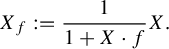 $$ \begin{align*} X_{f} :=\frac{1}{1+X\cdot f}X. \end{align*} $$
-
(1) X and
$X_{f}$
share the same stationary points, while
$$ \begin{align*} \mathrm{Pole}(X_{f}) =\mathrm{Pole}(X)\cap(f')^{-1}(0)\cup(1+X\cdot f)^{-1}(0)\backslash\mathrm{Pole}(X). \end{align*} $$
-
(2) If the flow
$\Psi :z\mapsto \Phi _{X}^{f(z)}(z)$
at time f along X is locally holomorphic around some
$z\in U$
, then:-
(a)
(this particularly means that if
$$ \begin{align*} \frac{X\cdot\Psi}{1+X\cdot f} =X\circ\Psi \end{align*} $$
$\Psi $
is locally biholomorphic at
$z\in U$
, then
$\Psi ^{*}X=X_{f}$
around z);
-
(b)
where
$$ \begin{align*} \Psi\circ\Delta_{f} =\Delta\circ\Psi, \end{align*} $$
$\Delta _{f}$
is the time-1 map of
$X_{f}$
and
$\Delta $
is that of X (this particularly means that if
$\Psi $
is locally biholomorphic at
$z\in U$
, then
$\Psi ^{*}\Delta =\Delta _{f}$
around z).
-
-
(3)
$\Psi $
is locally holomorphic at all
$z\in U$
except maybe for
$z\in \mathrm {Pole}(X_{f})$
. In particular,
$\Psi $
is holomorphic on a neighbourhood of
$\text {Zero}(X)$
and
$\Psi |_{\text {Zero}(X)}=\mathrm {Id}$
.


Proof. (1) If $p\in \mathrm {Pole}(X)$
, then
$p\in \mathrm {Pole}(X)$
, then $X_{f}(p)=({1}/{f'(p)}){\partial }/{\partial z}$
, else a pole in
$X_{f}(p)=({1}/{f'(p)}){\partial }/{\partial z}$
, else a pole in $X_{f}$
can only come from a zero of
$X_{f}$
can only come from a zero of $1+X\cdot f$
.
$1+X\cdot f$
.
(2) (a) Using Lie’s formula $\Psi =\sum _{n=0}^{\infty }({f^{n}}/{n!})X\cdot ^{n}\mathrm {Id}$
, we derive formally
$\Psi =\sum _{n=0}^{\infty }({f^{n}}/{n!})X\cdot ^{n}\mathrm {Id}$
, we derive formally
 $$ \begin{align*} X_{f}\cdot\Psi & =\frac{1}{1+X\cdot f}X\cdot\sum_{n=0}^{\infty}\frac{f^{n}}{n!}X\cdot^{n}\mathrm{Id}\\& =\frac{1}{1+X\cdot f}\bigg(\sum_{n=0}^{\infty}\frac{f^{n}}{n!}X\cdot^{n+1}\mathrm{Id}+(X\cdot f)\frac{f^{n-1}}{(n-1)!}X\cdot^{n}\mathrm{Id}\bigg)\\& =\sum_{n=0}^{\infty}\frac{f^{n}}{n!}X\cdot^{n+1}\mathrm{Id}\\& =X\circ\Psi. \end{align*} $$
(b) The Lie formula again implies that
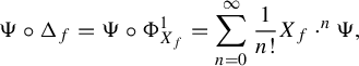 $$ \begin{align*} \Psi\circ\Delta_{f}=\Psi\circ\Phi_{X_{f}}^{1} =\sum_{n=0}^{\infty}\frac{1}{n!}X_{f}\cdot^{n}\Psi, \end{align*} $$
but a direct recursion yields $X_{f}\cdot ^{n}\Psi =(X\cdot ^{n}\mathrm {Id})\circ \Psi $
.
$X_{f}\cdot ^{n}\Psi =(X\cdot ^{n}\mathrm {Id})\circ \Psi $
.
(3) See Proposition 2.17 and subsequent remark.
Remark 2.20. Item (2) remains true for formal $f\in z\mathbb {C}[[z]] $
and formal
$f\in z\mathbb {C}[[z]] $
and formal $X\in z\mathbb {C}[[z]] {\partial }/{\partial z}$
(in that case,
$X\in z\mathbb {C}[[z]] {\partial }/{\partial z}$
(in that case, $\Psi $
is invertible as a formal transform at
$\Psi $
is invertible as a formal transform at $0$
).
$0$
).
Following the previous discussion, we define for $f\in \mathcal {S}$
, with
$f\in \mathcal {S}$
, with ![]() ,
,
 $$ \begin{align*} \Psi^{\pm} :z\longmapsto\Phi_{X_{0}}^{f^{\pm}(z)}(z). \end{align*} $$
Whenever $\Psi ^{\pm }$
is locally invertible, we have
$\Psi ^{\pm }$
is locally invertible, we have
 $$ \begin{align*} (\Psi^{\pm})^{*}X_{0} =X^{\pm} \end{align*} $$
by Proposition 2.19(1) with $X:=X_{0}$
.
$X:=X_{0}$
.
Lemma 2.21. Invoking the notation of Lemma 2.17, the mapping $\Psi ^{\pm }$
is locally biholomorphic on the holed-out domain
$\Psi ^{\pm }$
is locally biholomorphic on the holed-out domain $V^{\pm }\cap \mathcal {D}_{\unicode{x3bb} }$
and therefore conjugate
$V^{\pm }\cap \mathcal {D}_{\unicode{x3bb} }$
and therefore conjugate $X_{0}$
with
$X_{0}$
with $X^{\pm }=X_{f^{\pm }}$
.
$X^{\pm }=X_{f^{\pm }}$
.
Proof. Because $|f^{\pm }(z)|\leq 1$
for all
$|f^{\pm }(z)|\leq 1$
for all $z\in V^{\pm }$
, the construction of
$z\in V^{\pm }$
, the construction of $\mathcal {D}_{\unicode{x3bb} }$
guarantees that
$\mathcal {D}_{\unicode{x3bb} }$
guarantees that $\Phi _{X_{0}}^{f^{\pm }}$
is well defined and holomorphic on
$\Phi _{X_{0}}^{f^{\pm }}$
is well defined and holomorphic on $V^{\pm }\cap \mathcal {D}_{\unicode{x3bb} }$
. However, the poles of
$V^{\pm }\cap \mathcal {D}_{\unicode{x3bb} }$
. However, the poles of $X_{0}$
lie outside
$X_{0}$
lie outside $\mathcal {D}_{\unicode{x3bb} }$
; therefore, the conclusion follows from Proposition 2.19(3).
$\mathcal {D}_{\unicode{x3bb} }$
; therefore, the conclusion follows from Proposition 2.19(3).
From this lemma, we deduce that the dynamics of $X^{\pm }$
(governed by its sectorial spinal graph) is very close to that of
$X^{\pm }$
(governed by its sectorial spinal graph) is very close to that of $X_{0}|_{V^{\pm }}$
. A more quantitative analysis is conducted in §§5 and 6.1.
$X_{0}|_{V^{\pm }}$
. A more quantitative analysis is conducted in §§5 and 6.1.
3 Reduction
The proof of the next proposition, which reduces the problem of finding $\Delta $
to that of finding the pair
$\Delta $
to that of finding the pair $(f^{+},f^{-})$
in orbit space, is performed in §3.3. The definition of the functional space
$(f^{+},f^{-})$
in orbit space, is performed in §3.3. The definition of the functional space $\mathcal {S}$
is given in Definition 4.6 and the orbit space of the model vector field
$\mathcal {S}$
is given in Definition 4.6 and the orbit space of the model vector field $X_{0}$
is studied in detail in §3.1 below.
$X_{0}$
is studied in detail in §3.1 below.
Definition 3.1.
-
(1) We say that a holomorphic
$L:U\to \mathbb {C}$
is a first-integral of
$\Delta $
when
$$ \begin{align*} L\circ\Delta =L. \end{align*} $$
-
(2) A function
$H\neq 0$
holomorphic on V is a primitive function of X whenever
$$ \begin{align*} X\cdot H =2{i}\pi H. \end{align*} $$


Primitive functions H (actually unique up to a multiplicative constant) play a central role in the present study, because the Cousin problem $(\star )$
below comes from the structure of the ring of first-integrals of the map
$(\star )$
below comes from the structure of the ring of first-integrals of the map $\Delta $
. When U is a component of
$\Delta $
. When U is a component of $V^{\cap }$
, the primitive function H turns out to be a functional generator of the ring (Corollary 3.8): every first-integral L of
$V^{\cap }$
, the primitive function H turns out to be a functional generator of the ring (Corollary 3.8): every first-integral L of $\Delta $
factors holomorphically as
$\Delta $
factors holomorphically as $\phi \circ H$
. The latter property can be reworded equivalently as H gives a preferred coordinate on the space of orbits of
$\phi \circ H$
. The latter property can be reworded equivalently as H gives a preferred coordinate on the space of orbits of $\Delta $
.
$\Delta $
.
Remark 3.2. A primitive function H of X is indeed a first-integral of $\Delta $
(Lie formula):
$\Delta $
(Lie formula):
 $$ \begin{align*} H\circ\Delta =\sum_{n=0}^{+\infty}\frac{1}{n!}X\cdot^{n}H=\bigg(\sum_{n=0}^{+\infty}\frac{(2{i}\pi)^{n}}{n!}\bigg)H=H, \end{align*} $$
and hence any function of the form $\phi \circ H$
is a first-integral of
$\phi \circ H$
is a first-integral of $\Delta $
.
$\Delta $
.
Proposition 3.3. Take $f\in \mathcal {S}$
and fix
$f\in \mathcal {S}$
and fix $\unicode{x3bb}>0$
. Let
$\unicode{x3bb}>0$
. Let
 $$ \begin{align*} X_{}^{\pm} :=\frac{1}{1+X_{0}\cdot f^{\pm}}X_{0} \end{align*} $$
and $\Delta ^{\pm }$
be the time-1 map of
$\Delta ^{\pm }$
be the time-1 map of $X_{}^{\pm }$
. We write
$X_{}^{\pm }$
. We write $\Delta _{0}$
for the time-1 map of
$\Delta _{0}$
for the time-1 map of $X_{0}$
.
$X_{0}$
.
-
(1)
-
(a)
$\Delta ^{\pm }$
is holomorphic and bounded on and
$\Delta ^{\pm }(z)=\Delta _{0}(z)+\mathrm {o}(z^{3})$
near
$0\in \overline {V^{\pm }}$
. -
(b) Its space of orbits over
is canonically given by the range of the primitive function
$H_{}^{\pm }:=H_{0}\exp (2{i}\pi f^{\pm })$
, where is a primitive function of
$$ \begin{align*} H_{0}(z) :=\bigg(\frac{\unicode{x3bb} z}{1-z^{2}}\bigg)^{2{i}\pi\mu}\exp\bigg(-2{i}\pi\frac{1-z^{2}}{\unicode{x3bb} z}\bigg) \end{align*} $$
$X_{0}$
. Moreover, -
(c) For
$\sharp \in \{ 0,\infty \} $
, one has so that.
-
-
(2) The following properties are equivalent:
-
(a)
$\Delta ^{\pm }$
is the restriction to of a parabolic germ in ; -
(b)
$\Delta ^{+}=\Delta ^{-}$
on ; -
(c) the difference
$f^{-}-f^{+}$
is a first-integral of
$\Delta ^{+}$
; -
(d) there exists
,
$\sharp \in \{ 0,\infty \} $
, such that (⋆)
-
-
(3) Assume here that condition
$(\star )$
holds, so that .-
(a) The modulus of
$\Delta $
is . -
(b)
$(f^{+},f^{-})$
is the 1-sum of a formal power series
$F\in z\mathbb {C}[[z]] $
and
$\Delta $
is the time-1 map of
$({1}/({1+X_{0}\cdot F}))X_{0}$
.
-


3.1 Primitive function and space of orbits near
$0$

Define, by analytic continuation, the multivalued function over $\mathbb {C}\backslash \{ 0,\pm 1\} $
 $$ \begin{align*} H_{0}(z): =\exp(2{i}\pi t(z))=\bigg(\frac{\unicode{x3bb} z}{1-z^{2}}\bigg)^{2{i}\pi\mu}\exp\bigg(-2{i}\pi\frac{1-z^{2}}{\unicode{x3bb} z}\bigg), \end{align*} $$
with branch-cuts and determination indicated in Figure 9. By construction, it is a primitive function of $X_{0}$
:
$X_{0}$
:
 $$ \begin{align*} X_{0}\cdot H_{0} =2{i}\pi H_{0} \end{align*} $$
and the real-flow of $X_{0}$
corresponds to level curves of
$X_{0}$
corresponds to level curves of $|H_{0}|$
.
$|H_{0}|$
.
Definition 3.4. The cut sector $\widehat {V}$
is the complement
$\widehat {V}$
is the complement
 $$ \begin{align*} \widehat{V}^{\pm} :=V^{\pm}\backslash(\pm\mathbb{R}_{\geq1}) \end{align*} $$
on which $H_{0}$
is given the holomorphic determination induced by Figure 9 and written
$H_{0}$
is given the holomorphic determination induced by Figure 9 and written $H_{0}|_{\widehat {V}}$
. Notice that
$H_{0}|_{\widehat {V}}$
. Notice that
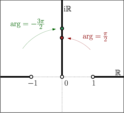
Figure 9 Branch-cut scheme of $H_{0}$
(cuts along fat lines) (colour online).
$H_{0}$
(cuts along fat lines) (colour online).
For every $z\in \widehat {V}$
such that
$z\in \widehat {V}$
such that $\Delta _{0}(z)\in \widehat {V}$
, one has
$\Delta _{0}(z)\in \widehat {V}$
, one has
 $$ \begin{align*} H_{0}(\Delta_{0}(z)) =H_{0}(z). \end{align*} $$
Moreover, the orbits of $\Delta _{0}|_{\widehat {V}}$
are in 2-to-
$\Delta _{0}|_{\widehat {V}}$
are in 2-to- $1$
correspondence with level sets of
$1$
correspondence with level sets of $H_{0}|_{\widehat {V}}$
, but the correspondence becomes 1-to-1 on
$H_{0}|_{\widehat {V}}$
, but the correspondence becomes 1-to-1 on ![]() . As
. As $z\to 0$
in
$z\to 0$
in $V^{\pm }$
, we have
$V^{\pm }$
, we have
and hence,
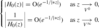
This particularly shows that $H_{0}(\widehat {V}^{\pm })=\mathbb {C}^{\times }$
: the sectorial space of orbits near
$H_{0}(\widehat {V}^{\pm })=\mathbb {C}^{\times }$
: the sectorial space of orbits near $0$
of
$0$
of $\Delta _{0}$
is a doubly punctured sphere,
$\Delta _{0}$
is a doubly punctured sphere,
the whole sphere $\overline {\mathbb {C}}$
being obtained by taking the closure
$\overline {\mathbb {C}}$
being obtained by taking the closure ![]() for
for $\sharp \in \{ 0,\infty \} $
.
$\sharp \in \{ 0,\infty \} $
.
Remark 3.5. Similarly, as $z\to \infty $
in
$z\to \infty $
in $V^{\pm }$
, we have
$V^{\pm }$
, we have
so that
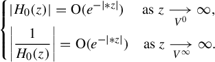
The (direct) monodromy of $H_{0}$
around
$H_{0}$
around $0$
is generated by the linear map
$0$
is generated by the linear map
 $$ \begin{align*} h \mapsto{e}^{-4\pi^{2}\mu}h. \end{align*} $$
Therefore, for the choice of the determination and branch-cuts we made, we have
which gives us a representation of the space of orbits of ![]() as
as
where $\overline {\mathbb {C}}\sqcup \overline {\mathbb {C}}$
stands for the abstract, disjoint union of two copies of
$\overline {\mathbb {C}}\sqcup \overline {\mathbb {C}}$
stands for the abstract, disjoint union of two copies of $\overline {\mathbb {C}}$
.
$\overline {\mathbb {C}}$
.
3.2 Sectorial orbit space and first-integrals
Here, we are particularly interested in the structure of the space of orbits of the sectorial time-1 maps $\Delta ^{\pm }$
of
$\Delta ^{\pm }$
of $X_{}^{\pm }$
. We wish to prove that these perturbations of
$X_{}^{\pm }$
. We wish to prove that these perturbations of $X_{0}$
still possess the properties underlined in §3.1 for the model, which is obtained via the sectorial normalization (§2.4).
$X_{0}$
still possess the properties underlined in §3.1 for the model, which is obtained via the sectorial normalization (§2.4).
Example 3.6. A Fatou coordinate of X is a locally biholomorphic mapping $\Psi $
such that
$\Psi $
such that
 $$ \begin{align*} \Psi^{*}\frac{\partial}{\partial z} =X. \end{align*} $$
This condition is equivalent to $X\cdot \Psi =1$
. Obviously, the Abel equation
$X\cdot \Psi =1$
. Obviously, the Abel equation $\Psi ^{*}\Delta =\mathrm {Id}+1$
holds whenever the time-1 map is defined, and we also speak of a Fatou coordinate for
$\Psi ^{*}\Delta =\mathrm {Id}+1$
holds whenever the time-1 map is defined, and we also speak of a Fatou coordinate for $\Delta $
.
$\Delta $
.
Let $H_{}^{\pm }:=H_{0}\exp (2{i}\pi f^{\pm })$
for
$H_{}^{\pm }:=H_{0}\exp (2{i}\pi f^{\pm })$
for $f\in \mathcal {S}$
. By construction,
$f\in \mathcal {S}$
. By construction, $H_{}^{\pm }$
is a primitive function of
$H_{}^{\pm }$
is a primitive function of $X_{}^{\pm }$
:
$X_{}^{\pm }$
:
 $$ \begin{align*} X_{}^{\pm}\cdot H_{}^{\pm} & =\frac{1}{1+X_{0}\cdot f^{\pm}}X_{0}\cdot H_{}^{\pm}=\frac{1}{1+X_{0}\cdot f^{\pm}}(X_{0}\cdot H_{0}+2{i}\pi H_{0}X_{0}\cdot f^{\pm})\exp(2{i}\pi f^{\pm})\\ & =2{i}\pi H_{}^{\pm}. \end{align*} $$
Hence, $({1}/{2{i}\pi })\log H_{}^{\pm }$
is a (sectorial) Fatou coordinate of
$({1}/{2{i}\pi })\log H_{}^{\pm }$
is a (sectorial) Fatou coordinate of $X_{}^{\pm }$
on
$X_{}^{\pm }$
on $\widehat {V}^{\pm }$
.
$\widehat {V}^{\pm }$
.
3.2.1 Sectorial orbit space
According to §2.4, we have near ![]()
 $$ \begin{align*} X_{}^{\pm} =(\Phi_{X_{0}}^{f^{\pm}})^{*}X_{0} \end{align*} $$
and the sectorial dynamics of $X_{}^{\pm }$
(respectively of
$X_{}^{\pm }$
(respectively of $\Delta ^{\pm }$
) are conjugate to that of
$\Delta ^{\pm }$
) are conjugate to that of $X_{0}|_{V^{\pm }}$
(respectively of
$X_{0}|_{V^{\pm }}$
(respectively of $\Delta _{0}|_{V^{\pm }}$
). Because
$\Delta _{0}|_{V^{\pm }}$
). Because $X_{0}(0)=0$
, the mapping
$X_{0}(0)=0$
, the mapping $\Phi _{X_{0}}^{f^{\pm }}$
is tangent to the identity near
$\Phi _{X_{0}}^{f^{\pm }}$
is tangent to the identity near $0$
. We deduce at once the following result from the study performed above §2.3 by pullback. In particular, observe that the primitive function
$0$
. We deduce at once the following result from the study performed above §2.3 by pullback. In particular, observe that the primitive function $H_{}^{\pm }$
of
$H_{}^{\pm }$
of $X_{}^{\pm }$
(which provides the preferred coordinate on the orbit space of
$X_{}^{\pm }$
(which provides the preferred coordinate on the orbit space of $\Delta $
) is the pullback of
$\Delta $
) is the pullback of $H_{0}|_{V^{\pm }}$
by
$H_{0}|_{V^{\pm }}$
by $\Phi _{X_{0}}^{f^{\pm }}$
according to Lie’s formula (2.4):
$\Phi _{X_{0}}^{f^{\pm }}$
according to Lie’s formula (2.4):
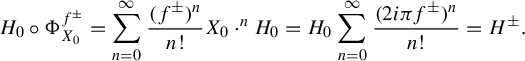 $$ \begin{align*} H_{0}\circ\Phi_{X_{0}}^{f^{\pm}} =\sum_{n=0}^{\infty}\frac{(f^{\pm})^{n}}{n!}X_{0}\cdot^{n}H_{0}=H_{0}\sum_{n=0}^{\infty}\frac{(2{i}\pi f^{\pm})^{n}}{n!}=H_{}^{\pm}. \end{align*} $$
In that sense, $\Delta ^{\pm }$
and
$\Delta ^{\pm }$
and $\Delta _{0}|_{V^{\pm }}$
share the same canonical orbital coordinate, a fact we summarize below.
$\Delta _{0}|_{V^{\pm }}$
share the same canonical orbital coordinate, a fact we summarize below.
Lemma 3.7. Let $f^{\pm }$
be holomorphic on
$f^{\pm }$
be holomorphic on $V^{\pm }$
with continuous extension to
$V^{\pm }$
with continuous extension to $\overline {\mathbb {C}}$
. Define
$\overline {\mathbb {C}}$
. Define $X_{}^{\pm }:=({1}({1+X_{0}\cdot f^{\pm }}))X_{0}$
and
$X_{}^{\pm }:=({1}({1+X_{0}\cdot f^{\pm }}))X_{0}$
and $H_{}^{\pm }:=H_{0}\times \exp (2{i}\pi f^{\pm })$
. There exists
$H_{}^{\pm }:=H_{0}\times \exp (2{i}\pi f^{\pm })$
. There exists ![]() such that the following assertions hold.
such that the following assertions hold.
-
(1) The time-1 map
$\Delta ^{\pm }$
of
$X_{}^{\pm }$
is holomorphic and injective on
$V^{\pm }\cap \mathcal {V}$
. Moreover,
$\Delta ^{\pm }(z)=\Delta _{0}(z)+\mathrm {o}(z^{3})$
near
$0$
in
$V^{\pm }$
. -
(2)
$H^{\pm }(V^{\pm }\cap \mathcal {V})=\mathbb {C}^{\times }$
and for
$\sharp \in \{ 0,\infty \} $
. -
(3) There exists a bijection between orbits of
$\Delta ^{\pm }$
on
$V^{\pm }\cap \mathcal {V}$
and level sets of
$H^{\pm }|_{V^{\pm }\cap \mathcal {V}}$
.


3.2.2 Sectorial primitive first-integrals
Corollary 3.8. Let U be an open subsector of $V^{\pm }$
attached to
$V^{\pm }$
attached to $0$
. The primitive function
$0$
. The primitive function $H_{}^{\pm }$
of X is a primitive first-integral of
$H_{}^{\pm }$
of X is a primitive first-integral of $\Delta ^{\pm }$
, in the sense that any first-integral L of
$\Delta ^{\pm }$
, in the sense that any first-integral L of $\Delta ^{\pm }$
on U factors as
$\Delta ^{\pm }$
on U factors as
 $$ \begin{align*} L =g\circ H_{}^{\pm} \end{align*} $$
for some g holomorphic on $H_{}^{\pm }(U)$
. (The converse is trivial.)
$H_{}^{\pm }(U)$
. (The converse is trivial.)
Proof. Let L be such that $L\circ \Delta =L$
. Then, it induces a holomorphic function
$L\circ \Delta =L$
. Then, it induces a holomorphic function $g:h\mapsto g(h)$
on the orbit space
$g:h\mapsto g(h)$
on the orbit space ![]() . According to the previous lemma, this space embeds as
. According to the previous lemma, this space embeds as $H_{}^{\pm }(U)\subset \mathbb {C}^{\times }$
. Therefore, we can assume that the coordinate h is given by
$H_{}^{\pm }(U)\subset \mathbb {C}^{\times }$
. Therefore, we can assume that the coordinate h is given by $H_{}^{\pm }$
, i.e.
$H_{}^{\pm }$
, i.e. $L=g\circ H_{}^{\pm }$
.
$L=g\circ H_{}^{\pm }$
.
3.3 Reduction: proof of Proposition 3.3
3.3.1 Item 1: sectorial dynamics and orbit space
This is the content of Lemma 3.7, and hence the item is proved.
3.3.2 Item 2: gluing condition
-
(a)⇒(b) This is trivial.
-
(b)⇒(a) The condition
$\Delta ^{-}=\Delta ^{+}$
guarantees that both sectorial functions glue to form a holomorphic germ, still called
$\Delta $
, on a punctured neighbourhood of
$0$
. As
$\Delta $
is bounded, Riemann’s theorem on removable singularity applies:
$\Delta $
extends holomorphically to . Finally, since
$\Delta _{0}(z)=z+\unicode{x3bb} z^{2}+\mathrm {o}(z^{2})$
(Lemma 2.4) and
$\Psi $
fixes
$0$
, we conclude . -
(c)⇒(b) The time-1 map of
$X_{}^{\pm }$
is
$\Delta ^{-}$
with primitive first-integral
$H_{f}^{-}= H_{0}\exp (2{i}\pi f^{-})=H_{f}^{+}\times \exp (2{i}\pi (f^{-}-f^{+}))$
. Hence,
$H_{f}^{-}$
is a first-integral of
$\Delta ^{+}$
as well as of
$\Delta ^{-}$
. Take
$z\in V^{\cap }$
a point where both
$\Delta ^{-}$
and
$\Delta ^{+}$
are defined (this property holds on some bounded subsector ). Then, which means that
$$ \begin{align*} H_{f}^{-}(\Delta^{+}(z)) & =H_{f}^{-}(z)\\ & =H_{f}^{-}(\Delta^{-}(z)), \end{align*} $$
$\Delta ^{+}=(\Delta ^{-})^{\circ \ell }$
for some
$\ell \in \mathbb {Z}$
, since orbits of
$\Delta ^{-}$
are in
$1$
-to-
$1$
correspondence with level sets of
$H_{f}^{-}$
. The integer
$\ell $
may depend on z, but Baire’s category theorem together with the principle of analytic continuation assert that
$\ell $
does actually not.
On the one hand,
$\Delta ^{+}$
and
$\Delta ^{-}$
coincide with
$\Delta _{0}$
up to
$\mathrm {o}(z^{3})$
, while on the other hand,
$\Delta _{0}^{\circ \ell }(z)=z+\ell \unicode{x3bb} z^{2}+\mathrm {o}(z^{2})$
for all . Thus,
$\ell =1$
and
$\Delta ^{+}=\Delta ^{-}$
on
$V^{\cap }$
. -
(b)⇒(c) The previous argument can actually be read backwards too.
-
(c)⇒(d) This is the content of Corollary 3.8.


3.3.3 Item 3: realization
-
(a) By construction, the Écalle–Voronin modulus of
$\Delta $
satisfies Replacing
$H_{}^{\pm }$
by
$H_{0}\exp (2{i}\pi f^{\pm })$
, then by and by brings the previous system into condition
$(\star )$
.
-
(b) Near
$0$
in , the function
$H_{}^{\pm }$
is 1-flat according to equation (3.1): for some choice of
$$ \begin{align*} |H_{}^{\pm}(z)| & \leq|H_{0}(z)|\exp(2\pi|f^{\pm}(z)|)\\ & \leq\exp\bigg(2\pi-\frac{\varepsilon}{|z|}\bigg) \end{align*} $$
(3.5)since
$$ \begin{align} 0<\varepsilon \leq\frac{5}{\unicode{x3bb}}<\frac{2\pi\cos({\pi}/{8})}{\unicode{x3bb}} \end{align} $$
$\unicode{x3bb} \leq 1$
. Because , the composition is also 1-flat at
$0$
, with the same 1-type. Therefore,
$f^{-}-f^{+}$
is 1-flat at
$0$
in , with the same 1-type. The same argument also applies in (beware that is embodied as a convergent power series in
${1}/{H_{f}^{+}}$
). Then, the Ramis–Sibuya theorem [Reference Loday-RichaudLR16, Theorem 5.2.1] asserts exactly that
$(f^{+},f^{-})$
is the 1-sum of some
$F\in z\mathbb {C}[[z]] $
. Being a
$1$
-sum is stable by differentiation so that
$(X_{0}\cdot f^{+},X_{0}\cdot f^{-})$
is a
$1$
-sum of
$X_{0}\cdot F$
, with the same 1-type. Hence,
$(\Phi _{X_{0}}^{f^{+}},\Phi _{X_{0}}^{f^{-}})$
is locally a
$1$
-sum of
$\Psi :=\Phi _{X_{0}}^{F}$
(according to Lemma 2.19), from which follows that
$(\Delta ^{+},\Delta ^{-})$
is a
$1$
-sum of (Here, the notion of
$$ \begin{align*} \Phi_{X}^{1} =\Psi^{*}\Delta_{0}. \end{align*} $$
$1$
-sum differs from that stated in the introduction in that we only have the holomorphy of
$\Psi ^{\pm }$
on a small sectorial region near
$0$
. This is sufficient, though.) Since
$\Delta ^{+}=\Delta ^{-}$
is a convergent power series at
$0$
, it can only mean that
$\Delta =\Phi _{X}^{1}$
.


4 Synthesis
We begin with fixing a formal class $\mu \in \mathbb {C}$
in
$\mu \in \mathbb {C}$
in ![]() (then
(then ![]() must be tangent to the linear map
must be tangent to the linear map ${e}^{4\pi ^{2}\mu }\mathrm {Id}$
) and pick an analytic data
${e}^{4\pi ^{2}\mu }\mathrm {Id}$
) and pick an analytic data

We wish to incarnate the abstract variable h as a concrete coordinate on a sectorial orbit space of a germ ![]() . To perform this task, we seek a pair of functions
. To perform this task, we seek a pair of functions $(H^{+},H^{-})$
 $$ \begin{align*} H^{\pm}:V^{\pm} \longrightarrow\mathbb{C}\subset\overline{\mathbb{C}} \end{align*} $$
whose range is biholomorphic to ${{ V^{\pm }}}/{{ \Delta }}$
and such that
${{ V^{\pm }}}/{{ \Delta }}$
and such that ![]() gives the transition between
gives the transition between $H^{+}$
and
$H^{+}$
and $H^{-}$
:
$H^{-}$
:
We recall that the two connected components of the intersection $V^{\cap }$
are sectors defined as in Figure 2 by
$V^{\cap }$
are sectors defined as in Figure 2 by $V^0 :=\left\{ z:\textrm{Im} (z)>0\right\} \cap V^{\cap}, V^\infty :=\left\{ z:\textrm{Im} (z)<0\right\} \cap V^{\cap}.$
Starting from a pair
the idea is to obtain $H^{\pm }$
as a perturbation
$H^{\pm }$
as a perturbation
 $$ \begin{align*} H_{}^{\pm} :=H_{0}\times\exp(2{i}\pi f^{\pm}),\quad f^{\pm}\in\mathcal{S} \end{align*} $$
of a primitive first-integral of the time-1 map $\Delta _{0}$
of the formal model
$\Delta _{0}$
of the formal model $X_{0}$
(see §2.3). According to Proposition 3.3, we need to solve the nonlinear Cousin problem
$X_{0}$
(see §2.3). According to Proposition 3.3, we need to solve the nonlinear Cousin problem
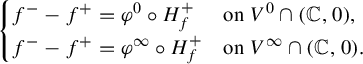
We introduce the Cauchy–Heine operator ![]() in §4.3, then prove it admits a unique fixed point in the unit ball of
in §4.3, then prove it admits a unique fixed point in the unit ball of $\mathcal {S}$
(§4.4). The latter is the sought solution of problem
$\mathcal {S}$
(§4.4). The latter is the sought solution of problem $(\star )$
.
$(\star )$
.
Remark 4.1. The proofs of all the technical lemmas involved below are to be found in §4.5.
4.1 Choice of the formal model and of the sectors
Before even considering solving the Cousin problem $(\star )$
, it should be well posed. In particular, the compositions
$(\star )$
, it should be well posed. In particular, the compositions ![]() and
and ![]() must make sense in the respective intersections
must make sense in the respective intersections ![]() and
and ![]() . This condition is not technical: for a genuine parabolic germ
. This condition is not technical: for a genuine parabolic germ $\Delta $
, a horn map is defined at least on the maximal domain of orbits that are sent by the local dynamics from one end of the sector
$\Delta $
, a horn map is defined at least on the maximal domain of orbits that are sent by the local dynamics from one end of the sector $V^{+}$
to the corresponding end of
$V^{+}$
to the corresponding end of $V^{-}$
.
$V^{-}$
.
Roughly speaking, this orbital domain is the range of the corresponding sectorial first-integral $H_{f}^{+}$
of the respective intersection’s component
$H_{f}^{+}$
of the respective intersection’s component ![]() or
or ![]() . To be able to gain control on its size, we impose the technical restriction
. To be able to gain control on its size, we impose the technical restriction
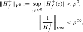
where ![]() and
and ![]() are the radius of convergence of
are the radius of convergence of ![]() and
and ![]() , the former as a power series in
, the former as a power series in ![]() and the latter in
and the latter in ![]() .
.
The natural idea that comes up is to use the 1-flatness of sectorial first-integrals at $0$
: on a small pair of sectors near
$0$
: on a small pair of sectors near $0$
, the above condition can be easily enforced. One then synthesizes
$0$
, the above condition can be easily enforced. One then synthesizes $\Delta $
on
$\Delta $
on ![]() in the preferred fashion (invoking Ahlfors–Bers theorem or directly by a holomorphic fixed-point). Treading on that path involves technical complications and other shortcomings, least of all the complete lack of a control on the form of the resulting germ
in the preferred fashion (invoking Ahlfors–Bers theorem or directly by a holomorphic fixed-point). Treading on that path involves technical complications and other shortcomings, least of all the complete lack of a control on the form of the resulting germ $\Delta $
. This, in turn, prevents any foreseeable statement about the uniqueness of
$\Delta $
. This, in turn, prevents any foreseeable statement about the uniqueness of $\Delta $
.
$\Delta $
.
To address the uniqueness question, one is therefore led to synthesize a global object $\Delta $
. However, one has to pay a price for it: any given model first-integral has a given range
$\Delta $
. However, one has to pay a price for it: any given model first-integral has a given range ![]() over
over ![]() , which cannot fit within the domain of every germ
, which cannot fit within the domain of every germ ![]() . Admittedly, one could contract the coordinate h by a linear map, but this would automatically increase the observed size of the orbital domain
. Admittedly, one could contract the coordinate h by a linear map, but this would automatically increase the observed size of the orbital domain ![]() near
near $\infty $
. Hence, only rare functions with
$\infty $
. Hence, only rare functions with ![]() bounded from below by the size of
bounded from below by the size of ![]() and
and ![]() can be realized as a perturbation of this first-integral.
can be realized as a perturbation of this first-integral.
Remark 4.2. In particular, when the data are unilateral (in Écalle’s terminology, meaning ![]() or
or ![]() ), it is possible to play the rescaling game on the orbits sphere and obtain a realization without caring about the parameter
), it is possible to play the rescaling game on the orbits sphere and obtain a realization without caring about the parameter $\unicode{x3bb} $
. The same holds if one of the components of
$\unicode{x3bb} $
. The same holds if one of the components of $\varphi $
is entire.
$\varphi $
is entire.
To drive the point home, we can obtain bounds for the primitive function
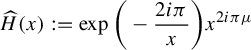 $$ \begin{align*} \widehat{H}(x) :=\exp\bigg(-\frac{2{i}\pi}{x}\bigg)x^{2{i}\pi\mu} \end{align*} $$
of the usual formal model $({x^{2}}/({1+\mu x})){\partial }/{\partial x}$
.
$({x^{2}}/({1+\mu x})){\partial }/{\partial x}$
.
Lemma 4.3. Define for $\tau \in \mathbb {C}^{\times }$
 $$ \begin{align*} \mathfrak{h}(\tau) :=\exp(-2{i}\pi(\tau+\mu\log\tau)). \end{align*} $$
For every $0<\delta <{\pi }/{2}$
, the following estimates hold:
$0<\delta <{\pi }/{2}$
, the following estimates hold:
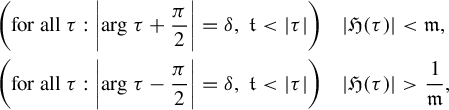 $$ \begin{align*} \bigg(\text{for all }\tau:\bigg\lvert\!\arg\tau+\frac{\pi}{2}\bigg\rvert=\delta,~\mathfrak{t}<|\tau|\bigg)\quad|\mathfrak{H}(\tau)| & <\mathfrak{m},\\\bigg(\text{for all }\tau:\bigg\lvert\!\arg\tau-\frac{\pi}{2}\bigg\rvert=\delta,~\mathfrak{t}<|\tau|\bigg)\quad|\mathfrak{H}(\tau)| &>\frac{1}{\mathfrak{m}}, \end{align*} $$
where
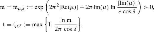 $$ \begin{align*} \mathfrak{m} & =\mathfrak{m}_{\mu,\delta}:=\exp\bigg(2\pi^{2}|\mathrm{Re}(\mu)|+2\pi\mathrm{Im}(\mu)\ln\frac{|\mathrm{Im}(\mu)|}{{e}\cos\delta}\bigg)>0,\\\mathfrak{t} & =\mathfrak{t}_{\mu,\delta}:=\max\bigg\{ 1,\frac{\ln\mathfrak{m}}{2\pi\cos\delta}\bigg\}. \end{align*} $$
We may think of $\tau $
as
$\tau $
as ${1}/{x}$
because
${1}/{x}$
because $\widehat {H}(x)=\mathfrak {h}({1}/{x})$
. Hence, the above estimate tells us that the size (in the coordinate
$\widehat {H}(x)=\mathfrak {h}({1}/{x})$
. Hence, the above estimate tells us that the size (in the coordinate $\widehat {H}$
) of the sectorial orbit spaces
$\widehat {H}$
) of the sectorial orbit spaces $\Omega _{0}$
and
$\Omega _{0}$
and $\Omega _{\infty }$
shrinks to
$\Omega _{\infty }$
shrinks to $0$
over increasingly smaller sectors of radius
$0$
over increasingly smaller sectors of radius ${1}/{\mathfrak {t}}\to 0$
. However, if we want to work on unbounded sectors covering
${1}/{\mathfrak {t}}\to 0$
. However, if we want to work on unbounded sectors covering $\mathbb {C}^{\times }$
, we cannot act on the smallness of the sectors any more; we must thereby find another way to control the size of the orbits domains to accommodate a given
$\mathbb {C}^{\times }$
, we cannot act on the smallness of the sectors any more; we must thereby find another way to control the size of the orbits domains to accommodate a given ![]() . This is done by performing the pullback of
. This is done by performing the pullback of $({x^{2}}/({1+\mu x})){\partial }/{\partial x}$
by a
$({x^{2}}/({1+\mu x})){\partial }/{\partial x}$
by a $1$
-parameter family of rational maps
$1$
-parameter family of rational maps $x:=\Pi (z)$
sending
$x:=\Pi (z)$
sending $V^{\cap }$
into sectors of size
$V^{\cap }$
into sectors of size ${1}/{\mathfrak {t}}=\mathrm {O}(\unicode{x3bb} )$
for which the previous lemma gives a bound
${1}/{\mathfrak {t}}=\mathrm {O}(\unicode{x3bb} )$
for which the previous lemma gives a bound $\mathfrak {m}\sim \exp (-{\mathrm {cst}}/{\unicode{x3bb} })$
.
$\mathfrak {m}\sim \exp (-{\mathrm {cst}}/{\unicode{x3bb} })$
.
Changing the variable $z\mapsto x=\Pi (z)$
in the usual formal model
$z\mapsto x=\Pi (z)$
in the usual formal model $({x^{2}}/({1+\mu x})){\partial }/{\partial x}$
results in a vector field whose time-
$({x^{2}}/({1+\mu x})){\partial }/{\partial x}$
results in a vector field whose time- $1$
flow has a first-integral of the form
$1$
flow has a first-integral of the form $\mathfrak {H}(\tau )$
for
$\mathfrak {H}(\tau )$
for $\tau =\tau (z):={1}/{\Pi (z)}$
. Namely, if
$\tau =\tau (z):={1}/{\Pi (z)}$
. Namely, if
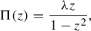 $$ \begin{align*} \Pi(z) =\frac{\unicode{x3bb} z}{1-z^{2}}, \end{align*} $$
then $({x^{2}}/({1+\mu x})){\partial }/{\partial x}$
is transformed into the
$({x^{2}}/({1+\mu x})){\partial }/{\partial x}$
is transformed into the $\sigma $
-invariant vector field
$\sigma $
-invariant vector field
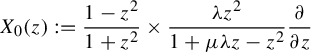 $$ \begin{align*} X_{0}(z) :=\frac{1-z^{2}}{1+z^{2}}\times\frac{\unicode{x3bb} z^{2}}{1+\mu\unicode{x3bb} z-z^{2}}\frac{\partial}{\partial z} \end{align*} $$
and $\tau $
into
$\tau $
into
 $$ \begin{align*} \tau=\tau_{\unicode{x3bb}}(z):= \frac{1-z^{2}}{\unicode{x3bb} z}, \end{align*} $$
yielding the first-integral
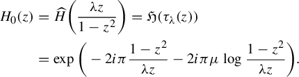 $$ \begin{align} H_{0}(z) & =\widehat{H}\bigg(\frac{\unicode{x3bb} z}{1-z^{2}}\bigg)=\mathfrak{H}(\tau_{\unicode{x3bb}}(z))\nonumber \\ & =\exp\bigg(-2{i}\pi\frac{1-z^{2}}{\unicode{x3bb} z}-2{i}\pi\mu\log\frac{1-z^{2}}{\unicode{x3bb} z}\bigg). \end{align} $$
Because $\tau \circ \sigma =\tau $
, all the above objects are
$\tau \circ \sigma =\tau $
, all the above objects are $\sigma $
-invariant. We establish now that this first-integral fulfils the expected properties on the pair of unbounded sectors
$\sigma $
-invariant. We establish now that this first-integral fulfils the expected properties on the pair of unbounded sectors $V^{\pm }$
. First, we ensure that
$V^{\pm }$
. First, we ensure that $\tau (V^{\cap })$
is included in an open sector of opening
$\tau (V^{\cap })$
is included in an open sector of opening ${\pi }/{2}$
with vertex at
${\pi }/{2}$
with vertex at $\infty $
.
$\infty $
.
Lemma 4.4. Fix $\unicode{x3bb} \leq 1$
and set
$\unicode{x3bb} \leq 1$
and set $\tau =\tau _{\unicode{x3bb} }(z):=({1-z^{2}})/{\unicode{x3bb} z}$
. Then,
$\tau =\tau _{\unicode{x3bb} }(z):=({1-z^{2}})/{\unicode{x3bb} z}$
. Then,
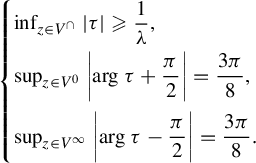
Second, we adapt the bounds of Lemma 4.3 for $\delta :={3\pi }/{8}$
to obtain the sought values of
$\delta :={3\pi }/{8}$
to obtain the sought values of $\mathfrak {m}_{\mu }$
and
$\mathfrak {m}_{\mu }$
and $\mathfrak {t}_{\mu }$
(we recall that
$\mathfrak {t}_{\mu }$
(we recall that $2\cos ({3\pi }/{8})=\sqrt {2-\sqrt {2}}$
):
$2\cos ({3\pi }/{8})=\sqrt {2-\sqrt {2}}$
):
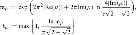 $$ \begin{align} \mathfrak{m}_{\mu} & :=\exp\bigg(2\pi^{2}|\mathrm{Re}(\mu)|+2\pi\mathrm{Im}(\mu)\ln\frac{4|\mathrm{Im}(\mu)|}{{e}\sqrt{2-\sqrt{2}}}\bigg),\\ \mathfrak{t}_{\mu} & :=\max\bigg\{ 1,\frac{\ln\mathfrak{m}_{\mu}}{\pi\sqrt{2-\sqrt{2}}}\bigg\} \nonumber \end{align} $$
as testified by the concluding result of this section.
Corollary 4.5. Pick $0<\unicode{x3bb} <({1}/{\mathfrak {t}_{\mu }})$
and define
$0<\unicode{x3bb} <({1}/{\mathfrak {t}_{\mu }})$
and define
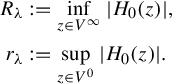
The following estimate holds:
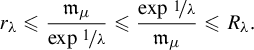
In fact, one has more precisely
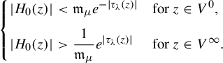
Proof. The constants $\mathfrak {m}_{\mu }^{2}$
and
$\mathfrak {m}_{\mu }^{2}$
and $\mathfrak {t}_{\mu }$
are related to that of Lemma 4.3 but for
$\mathfrak {t}_{\mu }$
are related to that of Lemma 4.3 but for $2\mu $
. Indeed, we have for
$2\mu $
. Indeed, we have for $\lvert \arg ({\tau }/{{i}})\rvert <{3\pi }/{8}$
:
$\lvert \arg ({\tau }/{{i}})\rvert <{3\pi }/{8}$
:
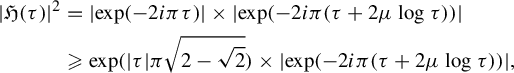 $$ \begin{align*} |\mathfrak{H}(\tau)|^{2} & =|\!\exp(-2{i}\pi\tau)|\times|\!\exp(-2{i}\pi(\tau+2\mu\log\tau))|\\ & \geq\exp(|\tau|\pi\sqrt{2-\sqrt{2}})\times|\!\exp(-2{i}\pi(\tau+2\mu\log\tau))|, \end{align*} $$
which becomes (since $\pi \sqrt {2-\sqrt {2}}>2$
)
$\pi \sqrt {2-\sqrt {2}}>2$
)
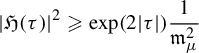 $$ \begin{align*} |\mathfrak{H}(\tau)|^{2} \geq\exp(2|\tau|)\frac{1}{\mathfrak{m}_{\mu}^{2}} \end{align*} $$
whenever $|\tau |>\mathfrak {t}_{\mu }$
. The latter condition is ensured as soon as
$|\tau |>\mathfrak {t}_{\mu }$
. The latter condition is ensured as soon as ${1}/{\unicode{x3bb} }>t_{\mu }$
thanks to Lemma 4.4. Under this hypothesis, we finally obtain
${1}/{\unicode{x3bb} }>t_{\mu }$
thanks to Lemma 4.4. Under this hypothesis, we finally obtain
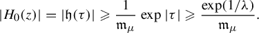 $$ \begin{align*} |H_{0}(z)|=|\mathfrak{h}(\tau)| \geq\frac{1}{\mathfrak{m}_{\mu}}\exp|\tau|\geq\frac{\exp({1}/{\unicode{x3bb}})}{\mathfrak{m}_{\mu}}. \end{align*} $$
The case $\lvert \arg ({\tau }/{-{i}})\rvert <{3\pi }/{8}$
is similar.
$\lvert \arg ({\tau }/{-{i}})\rvert <{3\pi }/{8}$
is similar.
4.2 Functions adapted to data
Let us translate in functions space the previous discussion.
Definition 4.6. As in the beginning of the section, we define the intersection
-
(1) Let
$U\subset \mathbb {C}$
be a domain. We introduce the Banach space of holomorphic, bounded functions f on U with continuous extension to the closure
$\overline {U}$
, equipped with the sup norm -
(2) As a particular case, we will be interested in
-
(3) We define
$\mathcal {S}$
as the space of pairs
$f=(f^{+},f^{-})$
with 1-flat difference in
$V^{\cap }$
and bounded
$1$
-type, both at
$0$
and
$\infty $
: equipped with the canonical product Banach norm. We denote by
$$ \begin{align*} \mathcal{S} :=\big\{ f\kern1.4pt{\in}\kern1.4pt\mathcal{S}(V^{+})\kern1.4pt{\times}\mathcal{S}(V^{-}):\limsup_{z^{\pm1}\to0}|z|^{\pm1}\ln|f^{-}(z)-f^{+}(z)|\kern1.4pt{\leq}\kern1.4pt-6\text{ for }z\in V^{\cap}\big\} , \end{align*} $$
$\mathcal {B}$
its unit ball.
-
(4) For
$f\in \mathcal {S}$
, we define the associated sectorial first-integral
$H_{f}=(H_{f}^{+},H_{f}^{-})$
given by
$$ \begin{align*} H_{}^{\pm} :=H_{0}\exp(2{i}\pi f^{\pm}). \end{align*} $$
-
(5) Let
be given. We say that
$(\unicode{x3bb} ,f)$
is adapted to
$\varphi $
whenever is included in the (open) disc of convergence of for
$\sharp \in \{ 0,\infty \} $
. We define for all
$\unicode{x3bb}>0$


We have, with a corresponding estimate for ![]() :
:
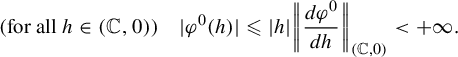
Proposition 4.7. Choose data ![]() . The subspace
. The subspace ![]() is an open set of
is an open set of $\mathcal {S}$
and if
$\mathcal {S}$
and if $\unicode{x3bb} $
is small enough, then it contains the unit ball:
$\unicode{x3bb} $
is small enough, then it contains the unit ball:
More generally, being given $f\in \mathcal {S}$
, it is always possible to take
$f\in \mathcal {S}$
, it is always possible to take $\unicode{x3bb} $
small enough to ensure that
$\unicode{x3bb} $
small enough to ensure that ![]() . (The following remark gives quantitative bounds.)
. (The following remark gives quantitative bounds.)
Remark 4.8. Denote by $\rho ^{\sharp }\in ]0,+\infty ]$
for
$\rho ^{\sharp }\in ]0,+\infty ]$
for $\sharp \in \{ 0,\infty \} $
the radius of convergence of
$\sharp \in \{ 0,\infty \} $
the radius of convergence of $\varphi ^{\sharp }$
. Quantitatively, the following conditions ensure that
$\varphi ^{\sharp }$
. Quantitatively, the following conditions ensure that ![]() :
:
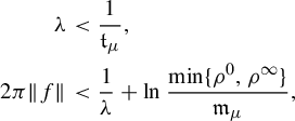
since according to Corollary 4.5, this implies
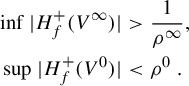
In particular, ![]() .
.
Proof. The mapping ![]() is continuous, and for each
is continuous, and for each ![]() , the set
, the set ![]() is compact. Thus,
is compact. Thus, ![]() is open in
is open in $\mathcal {S}$
. The remark just above precisely states that for any
$\mathcal {S}$
. The remark just above precisely states that for any $r>0$
, the ball
$r>0$
, the ball $r\mathcal {B}$
is included in
$r\mathcal {B}$
is included in ![]() whenever
whenever
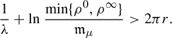
4.3 Cauchy–Heine transform
Now that $H_{0}$
and the sectors have been defined, we tackle the Cousin problem itself with data
$H_{0}$
and the sectors have been defined, we tackle the Cousin problem itself with data ![]() as in problem
as in problem $(\star )$
. Let us define the integral transform, which is the key to the construction.
$(\star )$
. Let us define the integral transform, which is the key to the construction.
Definition 4.9. Let ![]() be given. Assume that
be given. Assume that $(\unicode{x3bb} ,f)$
is adapted to it. Let
$(\unicode{x3bb} ,f)$
is adapted to it. Let $a^{\pm },~b^{\pm }$
be the outward-going half-lines making up the boundary
$a^{\pm },~b^{\pm }$
be the outward-going half-lines making up the boundary $\partial V^{\pm }$
as in Figure 10. We define
$\partial V^{\pm }$
as in Figure 10. We define $\Lambda _{f}:=(\Lambda _{f}^{+},\Lambda _{f}^{-})$
, where
$\Lambda _{f}:=(\Lambda _{f}^{+},\Lambda _{f}^{-})$
, where
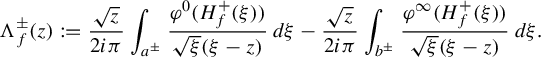

Figure 10 Integration paths used in the Cauchy–Heine transform (colour online).
Before stating anything about $\Lambda _{f}$
, we need to get convinced that it is well defined. For the sake of example, let us deal with the
$\Lambda _{f}$
, we need to get convinced that it is well defined. For the sake of example, let us deal with the $\int _{a}$
-part. According to the identity (4.3), we may find some
$\int _{a}$
-part. According to the identity (4.3), we may find some $C=\|{\mathit {d}\varphi }/{\mathit {d}h}\|_{H_{f}^{+}(V^{\cap })}\geq 0$
such that for all
$C=\|{\mathit {d}\varphi }/{\mathit {d}h}\|_{H_{f}^{+}(V^{\cap })}\geq 0$
such that for all $h\in H_{f}^{+}(a^{\pm })$
, we have
$h\in H_{f}^{+}(a^{\pm })$
, we have
Since we have for all $\xi \in a$
,
$\xi \in a$
,
and because $|H_{0}|$
is flat at
$|H_{0}|$
is flat at $0$
and
$0$
and $\infty $
along
$\infty $
along $a^{\pm }$
and
$a^{\pm }$
and $b^{\pm }$
, the integrals defining
$b^{\pm }$
, the integrals defining $\Lambda _{f}^{\pm }$
are absolutely convergent. That being said, as we want to control the magnitude of
$\Lambda _{f}^{\pm }$
are absolutely convergent. That being said, as we want to control the magnitude of $|\Lambda _{f}^{\pm }|$
with respect to both the point
$|\Lambda _{f}^{\pm }|$
with respect to both the point $z\in V^{\pm }$
and the parameter
$z\in V^{\pm }$
and the parameter $\unicode{x3bb} $
, we need to work a little bit more.
$\unicode{x3bb} $
, we need to work a little bit more.
Lemma 4.10. The model first-integral $H_{0}$
as given in equation (4.1) satisfies
$H_{0}$
as given in equation (4.1) satisfies
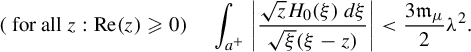 $$ \begin{align*} (\text{ for all } z:\mathrm{Re}(z)\geq0)\quad\int_{a^{+}}\bigg|\frac{\sqrt{z}H_{0}(\xi)\,\mathit{d}\xi}{\sqrt{\xi}(\xi-z)}\bigg| <\frac{3\mathfrak{m}_{\mu}}{2}\unicode{x3bb}^{2}. \end{align*} $$
Identical bounds for $\int _{a^{-}}$
and
$\int _{a^{-}}$
and $\int _{b^{\pm }}$
also hold.
$\int _{b^{\pm }}$
also hold.
We are now ready to prove the main properties of the operator $\Lambda _{f}$
.
$\Lambda _{f}$
.
Proposition 4.11. Let ![]() be given and assume that
be given and assume that $(\unicode{x3bb} ,f)\in \mathbb {R}_{>0}\times \mathcal {S}$
is adapted to it. Let
$(\unicode{x3bb} ,f)\in \mathbb {R}_{>0}\times \mathcal {S}$
is adapted to it. Let $\Lambda _{f}^{\pm }$
be as in the definition and recall that
$\Lambda _{f}^{\pm }$
be as in the definition and recall that $\sigma $
is the involution
$\sigma $
is the involution $z\mapsto ({-1}/{z})$
.
$z\mapsto ({-1}/{z})$
.
-
(1) For all
$z\in V^{\pm }$
, we have
$$ \begin{align*} \Lambda_{f}^{\mp}\circ\sigma(z) =-\Lambda_{f\circ\sigma}^{\pm}(z). \end{align*} $$
-
(2) For all
$z\in V^{\cap }$
, we have -
(3)
and


Proof. (1) Since $H_{0}\circ \sigma =H_{0}$
, we have
$H_{0}\circ \sigma =H_{0}$
, we have $H_{f}^{\pm }\circ \sigma =H_{f\circ \sigma }^{\mp }$
. The rest follows from applying the straightforward change of variable
$H_{f}^{\pm }\circ \sigma =H_{f\circ \sigma }^{\mp }$
. The rest follows from applying the straightforward change of variable $u:=\sigma (\xi )$
, which permutes
$u:=\sigma (\xi )$
, which permutes $a^{\pm }\leftrightarrow -a^{\mp }$
and
$a^{\pm }\leftrightarrow -a^{\mp }$
and $b^{\pm }\leftrightarrow -b^{\mp }$
. If
$b^{\pm }\leftrightarrow -b^{\mp }$
. If $z\in V^{-}$
, we have
$z\in V^{-}$
, we have $\sigma (z)={-1}/{z}\in V^{+}$
and
$\sigma (z)={-1}/{z}\in V^{+}$
and
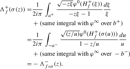
(2) This is a consequence of Cauchy’s formula. Assume for the sake of example that ![]() and pick
and pick $\varepsilon>0$
so small that
$\varepsilon>0$
so small that
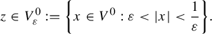
Hence (with the direct orientation on the boundary),
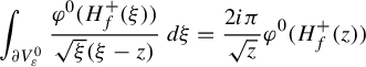
and with corresponding notation,
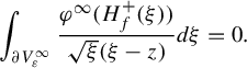
Because ![]() is exponentially flat near
is exponentially flat near $0$
and
$0$
and $\infty $
in the sector
$\infty $
in the sector ![]() , these identities hold at the limit
, these identities hold at the limit $\varepsilon \to 0$
, so that
$\varepsilon \to 0$
, so that

yields the expected result.
(3) When $z\in V^{+}$
with
$z\in V^{+}$
with $\mathrm {Re}(z)\geq 0$
, the bound
$\mathrm {Re}(z)\geq 0$
, the bound

is obtained by putting together the estimates of equations (4.3), (4.4) and twice Lemma 4.10 (once for a and once for b). According to item (1), the same argument proves the estimate for $|\Lambda _{f}^{-}(z)|$
when
$|\Lambda _{f}^{-}(z)|$
when $\mathrm {Re}(z)\leq 0$
and
$\mathrm {Re}(z)\leq 0$
and $z\in V^{-}$
.
$z\in V^{-}$
.
We must now deal with the case $z\in V^{+}$
and
$z\in V^{+}$
and $\mathrm {Re}(z)<0$
. We use the following trick: since we just proved that
$\mathrm {Re}(z)<0$
. We use the following trick: since we just proved that $|\Lambda _{f}^{-}(z)|$
satisfies the expected estimate on
$|\Lambda _{f}^{-}(z)|$
satisfies the expected estimate on $V^{-}$
and because
$V^{-}$
and because ![]() , we have
, we have
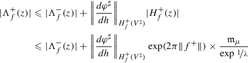
according to Corollary 4.5. The conclusion follows from ${1}/{\exp ({1}/{\unicode{x3bb} })}\leq 4\unicode{x3bb} ^{2}{e}^{-2}$
and
${1}/{\exp ({1}/{\unicode{x3bb} })}\leq 4\unicode{x3bb} ^{2}{e}^{-2}$
and $4{e}^{-2}+3<4$
.
$4{e}^{-2}+3<4$
.
Remark 4.12. Because $\int _{\partial V}({\varphi (H_{f}^{+}(\xi ))}/{\xi \sqrt {\xi }})\,\mathit {d}\xi $
is absolutely convergent,
$\int _{\partial V}({\varphi (H_{f}^{+}(\xi ))}/{\xi \sqrt {\xi }})\,\mathit {d}\xi $
is absolutely convergent, $\Lambda _{f}(z)$
is
$\Lambda _{f}(z)$
is $\mathrm {O}(\sqrt {z})$
as
$\mathrm {O}(\sqrt {z})$
as $z\to 0$
. In particular,
$z\to 0$
. In particular, $\Lambda _{f}(0)=0$
.
$\Lambda _{f}(0)=0$
.
Definition 4.13. We call

the Cauchy–Heine transform.
We deduce the following facts from the items of Proposition 4.11.
-
• From item (1) and thanks to the
$\sigma $
-action, we obtain Moreover, if f is a fixed-point of, then (4.5)
$$ \begin{align} f^{\pm}\circ\sigma =-f^{\mp}. \end{align} $$
-
•
solves the Cousin problem Moreover,
$(\Lambda _{f}^{+},\Lambda _{f}^{-})$
is
$1$
-flat with 1-type bounded from above by that of
$H_{f}^{+}$
, that is,
$-{6}/{\unicode{x3bb} }$
.
-
• From item (3), we derive the estimate
(4.6)


4.4 Convergence of the fixed-point method
From what we established in Proposition 4.11, we can derive more interesting properties of ![]() , which will allow us to iterate it provided
, which will allow us to iterate it provided $\unicode{x3bb} $
be small enough. Define for
$\unicode{x3bb} $
be small enough. Define for $\varphi \in h\mathbb {C}\{ h\} $
, and when it makes sense,
$\varphi \in h\mathbb {C}\{ h\} $
, and when it makes sense,
For given $\varphi $
, it decreases to
$\varphi $
, it decreases to $|\varphi '(0)|$
as
$|\varphi '(0)|$
as $\unicode{x3bb} \to 0$
. For given
$\unicode{x3bb} \to 0$
. For given $\unicode{x3bb}>0$
, it is a norm on the Banach space of bounded and holomorphic functions on the disc
$\unicode{x3bb}>0$
, it is a norm on the Banach space of bounded and holomorphic functions on the disc ![]() vanishing at
vanishing at $0$
. Moreover,
$0$
. Moreover, ![]() for all h in the disc.
for all h in the disc.
Proposition 4.14. Let $\mathcal {B}$
stand for the closed unit ball in the Banach space
$\mathcal {B}$
stand for the closed unit ball in the Banach space $\mathcal {S}$
(as in §4.2). Being given
$\mathcal {S}$
(as in §4.2). Being given ![]() , define
, define
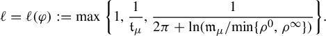
For $0<\unicode{x3bb} \leq \ell $
, let
$0<\unicode{x3bb} \leq \ell $
, let
(which is well defined since ![]() and
and ![]() are holomorphic and bounded on a disc of radius at least
are holomorphic and bounded on a disc of radius at least ![]() ). The transform
). The transform
is a well-defined $2\kappa _{\unicode{x3bb} }$
-Lipschitz map. In particular, if
$2\kappa _{\unicode{x3bb} }$
-Lipschitz map. In particular, if $\kappa _{\unicode{x3bb} }<\tfrac 12$
, then it is a contracting self-map of
$\kappa _{\unicode{x3bb} }<\tfrac 12$
, then it is a contracting self-map of $r_{\unicode{x3bb} }\mathcal {B}$
.
$r_{\unicode{x3bb} }\mathcal {B}$
.
Proof. Clearly, $\lim _{\unicode{x3bb} \to 0}\kappa _{\unicode{x3bb} }=0$
. The fact that
$\lim _{\unicode{x3bb} \to 0}\kappa _{\unicode{x3bb} }=0$
. The fact that ![]() ranges in
ranges in $r_{\unicode{x3bb} }\mathcal {B}$
comes from equation (4.6), since
$r_{\unicode{x3bb} }\mathcal {B}$
comes from equation (4.6), since ![]() .
.
Observe next that the assumption made on $\unicode{x3bb} $
guarantees that the condition
$\unicode{x3bb} $
guarantees that the condition ![]() is met, and hence,
is met, and hence,
because
Being given $f_{1},~f_{2}\in \mathcal {B}$
and
$f_{1},~f_{2}\in \mathcal {B}$
and ![]() , we thereby derive the bound:
, we thereby derive the bound:
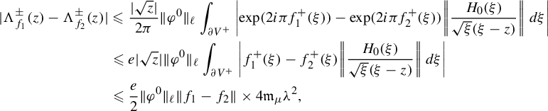
the last step coming from Lemma (4.10). Hence,
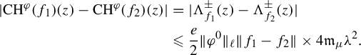
The case of ![]() is completely similar.
is completely similar.
Corollary 4.15. Let ![]() and take
and take
The map ![]() admits a unique fixed-point
admits a unique fixed-point $f\in \mathcal {B}$
, obtained for instance by considering the
$f\in \mathcal {B}$
, obtained for instance by considering the ![]() -orbit of
-orbit of $0$
. Moreover,
$0$
. Moreover,
Remark 4.16. The bound $\kappa _{\unicode{x3bb} }\exp (3368\kappa _{\unicode{x3bb} })\to 0$
is marginally sharper as
$\kappa _{\unicode{x3bb} }\exp (3368\kappa _{\unicode{x3bb} })\to 0$
is marginally sharper as $\unicode{x3bb} \to 0$
than
$\unicode{x3bb} \to 0$
than ![]() .
.
Proof. Well, this is just Banach’s theorem. The bound on the norm of the fixed-point f comes from the fact that
(Proposition 4.11) and that ![]() , while
, while $536\times 2\pi \simeq 3367.78<3368$
.
$536\times 2\pi \simeq 3367.78<3368$
.
4.5 Proof of the lemmas
4.5.1 Proof of Lemma 4.3
We need to bound $\mathfrak {H}$
on the half-lines
$\mathfrak {H}$
on the half-lines $\tau ={i} t\theta $
for
$\tau ={i} t\theta $
for $t>0$
and for fixed
$t>0$
and for fixed $\theta \in \mathbb {S}^{1}$
with
$\theta \in \mathbb {S}^{1}$
with $\arg \theta =\pm \delta $
. Define
$\arg \theta =\pm \delta $
. Define
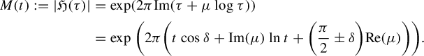 $$ \begin{align*} M(t):=|\mathfrak{H}(\tau)| & =\exp(2\pi\mathrm{Im}(\tau+\mu\log\tau))\\ & =\exp\bigg(2\pi\bigg(t\cos\delta+\mathrm{Im}(\mu)\ln t+\bigg(\frac{\pi}{2}\pm\delta\bigg)\mathrm{Re}(\mu)\bigg)\bigg). \end{align*} $$
An extremum is reached only if
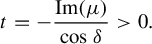 $$ \begin{align*} t =-\frac{\mathrm{Im}(\mu)}{\cos\delta}>0. \end{align*} $$
-
• If
$\mathrm{Im} (\mu )=0$
, the function M increases from
$M(0)$
to
$+\infty $
as t goes from
$0$
to
$+\infty $
: therefore,
$$ \begin{align*} M(0) =\exp\bigg(2\pi\mathrm{Re}(\mu)\bigg(\frac{\pi}{2}\pm\delta\bigg)\bigg)>\exp(\pi^{2}\mathrm{Re}(\mu)-\pi^{2}|\mathrm{Re}(\mu)|); \end{align*} $$
$M(0)\geq \exp (-2\pi ^{2}|\mathrm {Re}(\mu )|)={1}/{\mathfrak {m}}$
.
-
• If
$\mathrm{Im} (\mu )<0$
, the minimum of M is bounded from below by
$$ \begin{align*} M\bigg(-\frac{\mathrm{Im}(\mu)}{\cos\delta}\bigg) & \geq\exp\bigg(-2\pi\mathrm{Im}(\mu)\bigg(\ln\bigg|\frac{\mathrm{Im}(\mu)}{\cos\delta}\bigg|-1\bigg)+\pi^{2}\mathrm{Re}(\mu)-\pi^{2}|\mathrm{Re}(\mu)|\bigg)\\ & \geq\frac{1}{\mathfrak{m}}. \end{align*} $$
-
• If
$\mathrm{Im} (\mu )>0$
, the function M increases from
$0$
to
$+\infty $
as t runs along
$\mathbb {R}_{>0}$
. The unique
$t>0$
such that
$M(t)={1}/{\mathfrak {m}}$
satisfies If
$$ \begin{align*} \!t\cos\delta+\mathrm{Im}(\mu)\ln t {\kern-1pt}={\kern-1pt}\mathrm{Im}(\mu)\bigg({\kern-1pt}\!\ln\frac{\mathrm{Im}(\mu)}{\cos\delta}-1\!\bigg){\kern-1pt}+{\kern-1pt}\pi|\mathrm{Re}(\mu)|{\kern-1pt}-{\kern-1pt}\bigg(\frac{\pi}{2}\pm\delta{\kern-2pt}\bigg)\mathrm{Re}(\mu){\kern-1pt}\leq{\kern-1pt}\mathfrak{t}\cos\delta. \end{align*} $$
$t\geq 1$
, then
$t\cos \delta +\mathrm{Im} (\mu )\ln t\geq t\cos \delta $
; therefore, for all
$t>\mathfrak {t}$
, we have
$M(t)>M(\mathfrak {t})\geq {1}/{\mathfrak {m}}$
.


The case $t<0$
is taken care of similarly.
$t<0$
is taken care of similarly.
4.5.2 Proof of Lemma 4.4
Assume that $z=t\theta $
with
$z=t\theta $
with $t>0$
and
$t>0$
and $\theta :={i}{e}^{{i}\eta }$
for
$\theta :={i}{e}^{{i}\eta }$
for $\eta \in [-{\pi }/{8},{\pi }/{8}]$
, i.e.
$\eta \in [-{\pi }/{8},{\pi }/{8}]$
, i.e. ![]() . Then,
. Then,
 $$ \begin{align*} \arg\frac{\tau}{-{i}} =\arg(1+t^{2}{e}^{2{i}\eta})-\eta. \end{align*} $$
Because $-{\pi }/{2}<2\eta <{\pi }/{2}$
, we have
$-{\pi }/{2}<2\eta <{\pi }/{2}$
, we have
 $$ \begin{align*} \lvert\arg(1+t^{2}{e}^{2{i}\eta})\rvert \leq2\eta \end{align*} $$
and $\arg (1+t^{2}{e}^{2{i}\eta })\to _{+\infty }2\eta $
monotonically. On the one hand, we obtain, with sharp bounds,
$\arg (1+t^{2}{e}^{2{i}\eta })\to _{+\infty }2\eta $
monotonically. On the one hand, we obtain, with sharp bounds,
 $$ \begin{align*} -\frac{3\pi}{8}\leq-3\eta\leq \arg\frac{\tau}{-{i}}\leq\eta\leq3\eta\leq\frac{3\pi}{8}. \end{align*} $$
On the other hand,
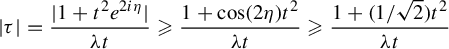 $$ \begin{align} |\tau| =\frac{|1+t^{2}{e}^{2{i}\eta}|}{\unicode{x3bb} t}\geq\frac{1+\cos(2\eta)t^{2}}{\unicode{x3bb} t}\geq\frac{1+({1}/{\sqrt{2}})t^{2}}{\unicode{x3bb} t} \end{align} $$
and basic calculus yields
 $$ \begin{align*} (\text{for all } t>0) \quad\frac{1+({1}/{\sqrt{2}})t^{2}}{\unicode{x3bb} t}\geq\frac{3}{\unicode{x3bb}\sqrt{2\sqrt{2}}}>\frac{1}{\unicode{x3bb}}. \end{align*} $$
4.5.3 Proof of Lemma (4.10)
For the sake of concision, we only deal with the case $\int _{a}({H_{0}(\xi )}/{\sqrt {\xi }(\xi -z)})\,\mathit {d}\xi $
, where
$\int _{a}({H_{0}(\xi )}/{\sqrt {\xi }(\xi -z)})\,\mathit {d}\xi $
, where $z\in U:=\{ z\neq 0:\mathrm {Re}(z)\geq 0\} $
and
$z\in U:=\{ z\neq 0:\mathrm {Re}(z)\geq 0\} $
and $a={e}^{{i}{5\pi }/{8}}\mathbb {R}_{>0}$
. For
$a={e}^{{i}{5\pi }/{8}}\mathbb {R}_{>0}$
. For $\mathrm {Re}(z)\geq 0$
, let us define
$\mathrm {Re}(z)\geq 0$
, let us define
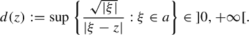 $$ \begin{align*} d(z) :=\sup\bigg\{ \frac{\sqrt{|\xi|}}{|\xi-z|}:\xi\in a\bigg\} \in\ ]0,+\infty[. \end{align*} $$
We have ${1}/{|\sqrt {\xi }(\xi -z)|}\leq {d(z)}/{|\xi |}$
so that writing
${1}/{|\sqrt {\xi }(\xi -z)|}\leq {d(z)}/{|\xi |}$
so that writing ![]() for
for $t>0$
yields
$t>0$
yields
 $$ \begin{align*} \bigg|\frac{H_{0}(\xi)\mathit{d}\xi}{\sqrt{\xi}(\xi-z)}\bigg| \leq\mathfrak{m}_{\mu}\,d(z)\times\frac{1}{t}\exp\frac{1+({1}/{\sqrt{2}})t^{2}}{-\unicode{x3bb} t}\,\mathit{d}t \end{align*} $$
(Corollary 4.5 and bound (4.7)), while
 $$ \begin{align*} \int_{0}^{+\infty}\frac{1}{t}\exp\bigg(-\frac{1}{\unicode{x3bb} t}-\frac{1}{\unicode{x3bb}\sqrt{2}}t\bigg)\,\mathit{d}t \leq\max_{t>0}\bigg(\frac{1}{t\exp({1}/{\unicode{x3bb} t})}\bigg)\int_{0}^{+\infty}\!\!\exp\bigg(-\frac{1}{\unicode{x3bb}\sqrt{2}}t\bigg)\,\mathit{d}t=\frac{\unicode{x3bb}}{{e}}\times\unicode{x3bb}\sqrt{2}. \end{align*} $$
To conclude, we need to bound $d(z)$
. First, we claim that
$d(z)$
. First, we claim that $|\xi -z|\geq |\xi -{i}|z||$
for all
$|\xi -z|\geq |\xi -{i}|z||$
for all $\xi \in a$
and
$\xi \in a$
and $\mathrm {Re}(z)\geq 0$
, so that we may as well assume that
$\mathrm {Re}(z)\geq 0$
, so that we may as well assume that $z\in {i}\mathbb {R}_{>0}$
. Next, elementary calculus provides the bound
$z\in {i}\mathbb {R}_{>0}$
. Next, elementary calculus provides the bound $d(z)\leq {1}/{\sqrt {2|z|}\sqrt {1-\cos ({\pi }/{8})}}$
, completing the proof since
$d(z)\leq {1}/{\sqrt {2|z|}\sqrt {1-\cos ({\pi }/{8})}}$
, completing the proof since ${1}/{{e}\sqrt {1-\cos ({\pi }/{8})}}<\tfrac 32$
.
${1}/{{e}\sqrt {1-\cos ({\pi }/{8})}}<\tfrac 32$
.
5 Globalization Theorem
This section is devoted to the proof of the Globalization Theorem. We prove items (1)–(3) in §5.3 below, but begin with establishing item (4) in §5.1, which introduces the needed material about the action of the involution $\sigma ={-1}/{\mathrm {Id}}$
.
$\sigma ={-1}/{\mathrm {Id}}$
.
Every object O involved in the paper comes as a pair of sectorial objects $O=(O^{+},O^{-})$
, each component being meromorphic on the corresponding
$O=(O^{+},O^{-})$
, each component being meromorphic on the corresponding $V^{\pm ~}$
. The action of
$V^{\pm ~}$
. The action of
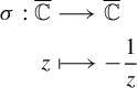 $$ \begin{align*} \sigma:\overline{\mathbb{C}} & \longrightarrow\overline{\mathbb{C}}\\ z & \longmapsto-\frac{1}{z} \end{align*} $$
on such objects is defined as
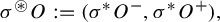 $$ \begin{align*} \sigma{}^{\circledast} O :=(\sigma^{*}O^{-},\sigma^{*}O^{+}), \end{align*} $$
where $\sigma ^{*}$
is just the usual action on holomorphic objects by change of coordinate:
$\sigma ^{*}$
is just the usual action on holomorphic objects by change of coordinate:
-
• on functions,
$\sigma ^{*}g:=g\circ \sigma $
; -
• on biholomorphisms,
$\sigma ^{*}\phi :=\sigma ^{\circ -1}\circ \phi \circ \sigma $
; -
• on vector fields,
$\sigma ^{*}X:=\mathrm {D}\sigma ^{-1}(X\circ \sigma )$
.


In what follows, every object will be $\sigma {}^{\circledast }$
-invariant:
$\sigma {}^{\circledast }$
-invariant:
 $$ \begin{align*} \sigma{}^{\circledast} O_{f} =O_{\sigma{}^{\circledast} f}, \end{align*} $$
as is the case, for example, of the sectorial first-integrals (because $H_{0}\circ \sigma =H_{0}$
, we have
$H_{0}\circ \sigma =H_{0}$
, we have $\sigma {}^{\circledast } H_{f}=H_{\sigma {}^{\circledast } f}$
), except for the Cauchy–Heine transform (Proposition 4.11 and identity (4.5)), which is
$\sigma {}^{\circledast } H_{f}=H_{\sigma {}^{\circledast } f}$
), except for the Cauchy–Heine transform (Proposition 4.11 and identity (4.5)), which is $\sigma {}^{\circledast }$
-antivariant since
$\sigma {}^{\circledast }$
-antivariant since ![]() .
.
5.1 Modulus at
$\infty $

Let $f\in \mathcal {B}$
in the unit ball of
$f\in \mathcal {B}$
in the unit ball of $\mathcal {S}$
give the parabolic realization
$\mathcal {S}$
give the parabolic realization $\Delta _{f}$
of some
$\Delta _{f}$
of some ![]() . According to Proposition 3.3, we know that
. According to Proposition 3.3, we know that $f^{-}-f^{+}$
is a first-integral of
$f^{-}-f^{+}$
is a first-integral of $\Delta _{f}$
on the whole
$\Delta _{f}$
on the whole $V^{\cap }$
, in particular, near
$V^{\cap }$
, in particular, near $\infty $
. Therefore, we can apply the converse of Proposition 3.3 to
$\infty $
. Therefore, we can apply the converse of Proposition 3.3 to $\sigma {}^{\circledast } f$
: there exists some parabolic germ
$\sigma {}^{\circledast } f$
: there exists some parabolic germ ![]() given by the sectorial time-1 map of
given by the sectorial time-1 map of $X_{\sigma {}^{\circledast } f}=\sigma {}^{\circledast } X_{f}$
(by uniqueness of the normal form).
$X_{\sigma {}^{\circledast } f}=\sigma {}^{\circledast } X_{f}$
(by uniqueness of the normal form).
By definition of the Birkhof–Écalle–Voronin modulus, it means that the identities
 $$ \begin{align*} \begin{cases} H_{f}^{-} =\psi_{f}\circ H_{f}^{+},\\ H_{\sigma{}^{\circledast} f}^{-} =\psi_{\sigma{}^{\circledast} f}\circ H_{\sigma{}^{\circledast} f}^{+} \end{cases} \end{align*} $$
hold on $V^{\cap }$
. By letting
$V^{\cap }$
. By letting $\sigma $
act on the first equality, we obtain
$\sigma $
act on the first equality, we obtain
 $$ \begin{align*} H_{\sigma{}^{\circledast} f}^{+}=H_{f}^{-}\circ\sigma=\psi_{f}\circ H_{f}^{+}\circ\sigma & =\psi_{f}\circ H_{\sigma{}^{\circledast} f}^{-}\\ & =\psi_{f}\circ\psi_{\sigma{}^{\circledast} f}\circ H_{\sigma{}^{\circledast} f}^{+}, \end{align*} $$
as expected.
5.2 Quantitative bounds for the dynamics of the model
$\Delta _{0}$

The first step to control precisely the dynamics of $X^{\pm }$
is to control that of
$X^{\pm }$
is to control that of $X_{0}$
and, more precisely, of
$X_{0}$
and, more precisely, of $\Phi _{X_{0}}^{\tau }$
for
$\Phi _{X_{0}}^{\tau }$
for $|\tau |\leq 1$
. We rely on the following technical lemma.
$|\tau |\leq 1$
. We rely on the following technical lemma.
Lemma 5.1. Let X be a holomorphic vector field on some pointed disc $\mathcal {D}:=\rho \mathbb {D}\backslash \{ 0\} $
and assume there exists some convenient constant
$\mathcal {D}:=\rho \mathbb {D}\backslash \{ 0\} $
and assume there exists some convenient constant $C>0$
such that for any
$C>0$
such that for any $0<r<\rho $
, we have
$0<r<\rho $
, we have
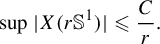 $$ \begin{align*} \sup|X(r\mathbb{S}^{1})| \leq\frac{C}{r}. \end{align*} $$
Pick $0<r<\rho $
and suppose moreover that
$0<r<\rho $
and suppose moreover that $0<\sqrt {r^{2}-2C}<\sqrt {r^{2}+2C}<\rho $
. Then:
$0<\sqrt {r^{2}-2C}<\sqrt {r^{2}+2C}<\rho $
. Then:
-
(1) for all
$|\tau |\leq 1$
, the mapping
$\Delta :=\Phi _{X}^{\tau }$
is holomorphic on a neighbourhood of
$r\mathbb {S}^{1}$
; -
(2)
$\Delta (r\mathbb {S}^{1})\subset \mathcal {D}$
.


Proof. This is a simple variational argument applied to $\phi (t):=|z(t)|^{2}$
for
$\phi (t):=|z(t)|^{2}$
for $t\in [0,\tau ]$
, where z solves
$t\in [0,\tau ]$
, where z solves $\dot {z}=X(z)$
. Indeed,
$\dot {z}=X(z)$
. Indeed, $\phi =z\overline {z}$
so that
$\phi =z\overline {z}$
so that
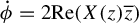 $$ \begin{align*} \dot{\phi} =2\mathrm{Re}(X(z)\overline{z}) \end{align*} $$
and
 $$ \begin{align*} |\dot{\phi}| \leq2C. \end{align*} $$
Integrating the left- and right-hand sides with respect to $t\in [0,1]$
, one obtains
$t\in [0,1]$
, one obtains
 $$ \begin{align*} r^{2}-2C\leq|z(\tau)|^{2} \leq r^{2}+2C.\\[-37pt] \end{align*} $$
We apply now this result to the model $X_{0}$
.
$X_{0}$
.
Lemma 5.2. Consider $\rho \leq {1}/{20}$
and assume that
$\rho \leq {1}/{20}$
and assume that $\unicode{x3bb} <\min \{ {1}/{2|\mu |},{\rho ^{2}}/{6}\} $
.
$\unicode{x3bb} <\min \{ {1}/{2|\mu |},{\rho ^{2}}/{6}\} $
.
-
(1) For each
$0<r<\rho $
and
$|z\pm {i}|=r$
, we have
$$ \begin{align*} |X_{0}(z)| <\frac{\unicode{x3bb}}{r}. \end{align*} $$
-
(2) If
$r:=2\sqrt {\unicode{x3bb} }$
and
$|\tau |\leq 1$
, then
$\Phi _{X_{0}}^{\tau }$
is holomorphic on the annulus
$\mathcal {A}_{\pm {i}}:=\pm {i}+\rho \mathbb {D}\backslash \overline {r\mathbb {D}}$
and
$\Phi _{X_{0}}^{\tau }(\mathcal {A}_{\pm {i}})\subset \pm {i}+\rho \mathbb {D}\backslash \{ 0\} $
.


Example 5.3. For instance, for $\rho :={1}/{20}$
, we can choose the disk
$\rho :={1}/{20}$
, we can choose the disk $D_{\pm {i}}$
in Proposition 2.17(2) to be of radius
$D_{\pm {i}}$
in Proposition 2.17(2) to be of radius $2\sqrt {\unicode{x3bb} }$
provided
$2\sqrt {\unicode{x3bb} }$
provided $\unicode{x3bb} <{1}/{2400}$
.
$\unicode{x3bb} <{1}/{2400}$
.
Proof. The proof for an annulus centred at $-{i}$
is identical to that of
$-{i}$
is identical to that of ${i}$
, so we only deal with that case.
${i}$
, so we only deal with that case.
(1) The dominant part of R near ${i}$
is given by
${i}$
is given by ${\unicode{x3bb} }/({1+z^{2}})$
. We use in the roughest possible fashion the triangular inequalities:
${\unicode{x3bb} }/({1+z^{2}})$
. We use in the roughest possible fashion the triangular inequalities:
-
•
$|z|^{2}\leq (1+\rho )^{2}$
; -
•
$\sqrt {2}-\rho <|1-z^{2}|\leq 1+(1+\rho ^{2})$
; -
•
$|1-z^{2}+\unicode{x3bb} \mu z|>(\sqrt {2}-\rho )^{2}-({1+\rho })/{2}$
, since
$\unicode{x3bb} |\mu ||z|<({1+\rho })/{2}$
; -
•
$|1+z^{2}|\geq r(2-\rho )$
;


finally yielding
 $$ \begin{align*} |X_{0}(z)| <\frac{\unicode{x3bb}}{r}. \end{align*} $$
(2) To apply Lemma 5.1, we must find r such that $0<r^{2}-2\unicode{x3bb} $
and
$0<r^{2}-2\unicode{x3bb} $
and $r^{2}+2\unicode{x3bb} <\rho ^{2}$
. The choice
$r^{2}+2\unicode{x3bb} <\rho ^{2}$
. The choice $r:=2\sqrt {\unicode{x3bb} }$
fulfils both conditions provided
$r:=2\sqrt {\unicode{x3bb} }$
fulfils both conditions provided $\unicode{x3bb} <{\rho ^{2}}/{6}$
.
$\unicode{x3bb} <{\rho ^{2}}/{6}$
.
To conclude this lemma, we recall Lemma 2.15. We just proved that no point form $\mathcal {C}$
can ever reach the pole
$\mathcal {C}$
can ever reach the pole ${i}$
in time
${i}$
in time $\tau $
, and hence
$\tau $
, and hence $\Phi _{X_{0}}^{\tau }$
must be holomorphic on
$\Phi _{X_{0}}^{\tau }$
must be holomorphic on $\mathcal {C}$
.
$\mathcal {C}$
.
We play the same game near the poles
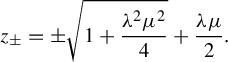 $$ \begin{align*} z_{\pm} =\pm\sqrt{1+\frac{\unicode{x3bb}^{2}\mu^{2}}{4}}+\frac{\unicode{x3bb}\mu}{2}. \end{align*} $$
Observe that if $\unicode{x3bb} <{1}/{2|\mu |}$
, then
$\unicode{x3bb} <{1}/{2|\mu |}$
, then
 $$ \begin{align} |z_{\pm}\mp1| <\frac{\unicode{x3bb}|\mu|}{2}+\frac{\unicode{x3bb}^{2}|\mu|^{2}}{8}<\unicode{x3bb}\frac{9|\mu|}{16}. \end{align} $$
In particular, $\tfrac 12<|z_{\pm }|<\tfrac 32$
.
$\tfrac 12<|z_{\pm }|<\tfrac 32$
.
Lemma 5.4. Consider $\rho \leq {1}/{20}$
and assume that
$\rho \leq {1}/{20}$
and assume that $\unicode{x3bb} <\min \{ {1}/{2|\mu |},{\rho ^{2}}/{32}\} $
.
$\unicode{x3bb} <\min \{ {1}/{2|\mu |},{\rho ^{2}}/{32}\} $
.
-
(1) For each
$0<r<\rho $
and
$|z-z_{\pm }|=r$
, we have
$$ \begin{align*} |X_{0}(z)| <\frac{8\unicode{x3bb}}{r}. \end{align*} $$
-
(2) If
$r:=4\sqrt {\unicode{x3bb} }$
and
$|\tau |\leq 1$
, then
$\Phi _{X_{0}}^{\tau }$
is holomorphic on the annulus
$\mathcal {A}_{\pm }:=z_{\pm }+\rho \mathbb {D}\backslash \overline {r\mathbb {D}}$
and
$\Phi _{X_{0}}^{\tau }(\mathcal {A}_{\pm })\subset z_{\pm }+\rho \mathbb {D}\backslash \{ 0\} $
.


Example 5.5. For instance, for $\rho :={1}/{20}$
, we can choose the disk
$\rho :={1}/{20}$
, we can choose the disk $D_{z_{\pm }}$
in Proposition 2.17(2) to be of radius
$D_{z_{\pm }}$
in Proposition 2.17(2) to be of radius $4\sqrt {\unicode{x3bb} }$
provided
$4\sqrt {\unicode{x3bb} }$
provided $\unicode{x3bb} <{1}/{12\,800}$
.
$\unicode{x3bb} <{1}/{12\,800}$
.
Proof. Again, we only deal with the neighbourhood of $z_{+}$
, and obtain the expected bound using
$z_{+}$
, and obtain the expected bound using $|z-z_{+}|=r$
:
$|z-z_{+}|=r$
:
-
•
$|z^{2}|\leq (\tfrac 32+\rho )^{2}$
; -
•
$|1-z^{2}|\leq 1+(\tfrac 32+\rho )^{2}$
; -
• (from equation (5.1))
$|z\pm {i}|\geq \sqrt {2}-\rho -{9}/{32}$
; -
•
$|1+\unicode{x3bb} \mu z-z^{2}|=r|2z_{+}+r|\geq r(1-\rho )$
.


5.3 Dynamics of
$X^{\pm }$

Here and in all the following, we take $f\in \mathcal {B}$
in the unit ball of
$f\in \mathcal {B}$
in the unit ball of $\mathcal {S}$
and suppose
$\mathcal {S}$
and suppose
 $$ \begin{align*} 0<\unicode{x3bb} <\min\bigg\{ \frac{1}{2|\mu|},\frac{1}{12\,800}\bigg\}. \end{align*} $$
Lemma 5.6. Each vector field $X^{-}$
and
$X^{-}$
and $X^{+}$
admits a unique pole in each disc
$X^{+}$
admits a unique pole in each disc $\pm {i}+3\sqrt {\unicode{x3bb} }\mathbb {D}$
, which is simple.
$\pm {i}+3\sqrt {\unicode{x3bb} }\mathbb {D}$
, which is simple.
Proof. For the sake of clarity, we choose a sector $V^{+}$
and let f stand for
$V^{+}$
and let f stand for $f^{+}$
, the case of
$f^{+}$
, the case of $f^{-}$
on
$f^{-}$
on $V^{-}$
being completely similar. Let
$V^{-}$
being completely similar. Let $\rho :=9\sqrt {\unicode{x3bb} }\leq {1}/{20}$
so that
$\rho :=9\sqrt {\unicode{x3bb} }\leq {1}/{20}$
so that $0<\unicode{x3bb} <{\rho ^{2}}/{6}$
and we can apply Lemma 5.2: for any
$0<\unicode{x3bb} <{\rho ^{2}}/{6}$
and we can apply Lemma 5.2: for any $0<r<\rho $
and
$0<r<\rho $
and $|z\pm {i}|=r$
, we have
$|z\pm {i}|=r$
, we have
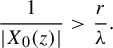 $$ \begin{align*} \frac{1}{|X_{0}(z)|}>\frac{r}{\unicode{x3bb}}. \end{align*} $$
In adddition, Cauchy’s formula applied to f on the circle $\pm {i}+\rho \mathbb {S}^{1}$
(which is included in
$\pm {i}+\rho \mathbb {S}^{1}$
(which is included in $V^{\cap }$
) yields for
$V^{\cap }$
) yields for $z\in \pm {i}+r\mathbb {S}^{1}$
 $$ \begin{align*} |f'(z)| \leq\frac{1}{2\pi}\oint_{{i}+r\mathbb{D}}\frac{|f(z)|}{|z-{i}|^{2}}|\mathit{d}z|\leq\frac{\rho}{(\rho-r)^{2}}. \end{align*} $$
Whenever ${\rho }/{(\rho -r)^{2}}<{r}/{\unicode{x3bb} }$
, we can apply Rouché’s theorem to the holomorphic functions
${\rho }/{(\rho -r)^{2}}<{r}/{\unicode{x3bb} }$
, we can apply Rouché’s theorem to the holomorphic functions ${1}/({X_{0}\cdot \mathrm {Id}})$
and
${1}/({X_{0}\cdot \mathrm {Id}})$
and ${1}/({X_{0}\cdot \mathrm {Id}})+f'$
on the disc
${1}/({X_{0}\cdot \mathrm {Id}})+f'$
on the disc $\pm {i}+r\mathbb {D}$
, so that
$\pm {i}+r\mathbb {D}$
, so that ${1}/({X_{0}\cdot \mathrm {Id}})+f'$
has a single simple zero in the disc. In other words,
${1}/({X_{0}\cdot \mathrm {Id}})+f'$
has a single simple zero in the disc. In other words, $({1}/({1+X_{0}\cdot f}))X_{0}$
has a single (simple) pole in the disc.
$({1}/({1+X_{0}\cdot f}))X_{0}$
has a single (simple) pole in the disc.
The condition ${\rho }/{(\rho{\kern-1pt} -{\kern-1pt}r)^{2}}{\kern-1pt}<{\kern-1pt}{r}/{\unicode{x3bb} }$
is equivalent to
${\rho }/{(\rho{\kern-1pt} -{\kern-1pt}r)^{2}}{\kern-1pt}<{\kern-1pt}{r}/{\unicode{x3bb} }$
is equivalent to $\phi (r){\kern-1pt}>{\kern-1pt}\unicode{x3bb} $
, where
$\phi (r){\kern-1pt}>{\kern-1pt}\unicode{x3bb} $
, where ${\phi {\kern-1pt}:{\kern-1pt}r{\kern-1pt}\mapsto{\kern-1pt} ({r}/{\rho })(r{\kern-1pt}-{\kern-1pt}\rho )^{2}}$
vanishes at
${\phi {\kern-1pt}:{\kern-1pt}r{\kern-1pt}\mapsto{\kern-1pt} ({r}/{\rho })(r{\kern-1pt}-{\kern-1pt}\rho )^{2}}$
vanishes at $0$
and
$0$
and $\rho $
. The function reaches its maximum
$\rho $
. The function reaches its maximum ${4\rho ^{2}}/{27}>\unicode{x3bb} $
at
${4\rho ^{2}}/{27}>\unicode{x3bb} $
at ${\rho }/{3}=:r$
.
${\rho }/{3}=:r$
.
A similar phenomenon happens near $z_{\pm }$
.
$z_{\pm }$
.
Lemma 5.7. The vector field $X^{\pm }$
admits a unique pole
$X^{\pm }$
admits a unique pole $p_{\pm }$
in the disc
$p_{\pm }$
in the disc $\pm 1+5\sqrt {\unicode{x3bb} }\mathbb {D}$
, which is simple.
$\pm 1+5\sqrt {\unicode{x3bb} }\mathbb {D}$
, which is simple.
Proof. This time, we take $\rho :=15\sqrt {\unicode{x3bb} }$
in Lemma 5.4 and apply Cauchy’s formula to the circle
$\rho :=15\sqrt {\unicode{x3bb} }$
in Lemma 5.4 and apply Cauchy’s formula to the circle $z_{\pm }+r\mathbb {S}^{1}$
, where
$z_{\pm }+r\mathbb {S}^{1}$
, where $0<r<\rho $
, so that, for every
$0<r<\rho $
, so that, for every $|z-z_{\pm }|=r$
,
$|z-z_{\pm }|=r$
,
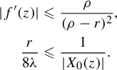 $$ \begin{align*} |f'(z)| & \leq\frac{\rho}{(\rho-r)^{2}},\\ \frac{r}{8\unicode{x3bb}} & \leq\frac{1}{|X_{0}(z)|}. \end{align*} $$
The condition $8\unicode{x3bb} <\phi (r)$
is met if
$8\unicode{x3bb} <\phi (r)$
is met if $r:=5\sqrt {\unicode{x3bb} }$
.
$r:=5\sqrt {\unicode{x3bb} }$
.
This proposition ends the proof of items (1)–(3) of the Globalization Theorem.
Proposition 5.8. Let us denote by $p_{{i}}^{\pm }$
,
$p_{{i}}^{\pm }$
, $p_{-{i}}^{\pm }$
and
$p_{-{i}}^{\pm }$
and $z_{\pm }$
the simple poles of
$z_{\pm }$
the simple poles of $X^{\pm }$
provided by the previous lemmas. The following properties hold.
$X^{\pm }$
provided by the previous lemmas. The following properties hold.
-
(1)
$X^{\pm }$
does not have any other pole in
$V^{\pm }$
. -
(2)
$p_{{i}}^{+}=p_{{i}}^{-}=:p_{{i}}$
and
$p_{-{i}}^{+}=p_{-{i}}^{-}:=p_{-{i}}$
. Moreover,
$\sigma (p_{{i}})=p_{-{i}}$
and
$\sigma (p_{+})=p_{-}$
. -
(3) The vector field
$X^{\pm }$
is conjugate to
$({1}/{w}){\partial }/{\partial w}$
as in Lemma 2.7 on a disc centred at p and containing the two attached ramification points
$\{ z_{p},w_{p}\} $
, and hence conjugates the monodromies of the time-1 maps.


Proof. (1) Recalling Proposition 2.19(3), the sectorial normalization $\Psi ^{\pm }$
between
$\Psi ^{\pm }$
between $X_{0}$
and
$X_{0}$
and $X^{\pm }$
is holomorphic on
$X^{\pm }$
is holomorphic on $\mathcal {D}_{\unicode{x3bb} }$
. If
$\mathcal {D}_{\unicode{x3bb} }$
. If $X^{\pm }$
were to admit a pole outside
$X^{\pm }$
were to admit a pole outside $\Psi ^{\pm }(\mathcal {D}_{\unicode{x3bb} })$
, it would show in
$\Psi ^{\pm }(\mathcal {D}_{\unicode{x3bb} })$
, it would show in $X_{0}$
. Since
$X_{0}$
. Since $\Psi ^{\pm }(\partial \mathcal {D}_{\unicode{x3bb} })$
lies within the union of the discs given by the two previous lemmas, this cannot be the case. Indeed, according to Lemma 5.2, the circle
$\Psi ^{\pm }(\partial \mathcal {D}_{\unicode{x3bb} })$
lies within the union of the discs given by the two previous lemmas, this cannot be the case. Indeed, according to Lemma 5.2, the circle $\pm {i}+2\sqrt {\unicode{x3bb} }\mathbb {S}^{1}$
is mapped by
$\pm {i}+2\sqrt {\unicode{x3bb} }\mathbb {S}^{1}$
is mapped by $\Psi ^{\pm }$
into a disc centred at
$\Psi ^{\pm }$
into a disc centred at $\pm {i}$
of radius
$\pm {i}$
of radius $\rho :=3\sqrt {\unicode{x3bb} }>r$
. The same goes accordingly near
$\rho :=3\sqrt {\unicode{x3bb} }>r$
. The same goes accordingly near $z_{\pm }$
.
$z_{\pm }$
.
(2) Recalling Lemma 2.15, which also holds locally for meromorphic vector fields, a pole p of $X^{+}$
induces two ramification points
$X^{+}$
induces two ramification points $\{ z_{p},w_{p}\} $
in
$\{ z_{p},w_{p}\} $
in $\Delta $
, which are mapped by
$\Delta $
, which are mapped by $\Delta $
to p. Since
$\Delta $
to p. Since $\Delta $
is also the time-1 map of
$\Delta $
is also the time-1 map of $X^{-}$
, the points
$X^{-}$
, the points $z_{p}$
and
$z_{p}$
and $w_{p}$
also belong to a stable manifold of
$w_{p}$
also belong to a stable manifold of $X^{-}$
and are sent to a pole of
$X^{-}$
and are sent to a pole of $X^{-}$
by its time-1 flow. Hence, p is also a pole of
$X^{-}$
by its time-1 flow. Hence, p is also a pole of $X^{-}$
.
$X^{-}$
.
For the very same reason that a pole of $X_{f}=(X^{+},X^{-})$
is a dynamical feature, the poles of
$X_{f}=(X^{+},X^{-})$
is a dynamical feature, the poles of $X_{\sigma {}^{\circledast } f}$
and that of
$X_{\sigma {}^{\circledast } f}$
and that of $\sigma {}^{\circledast } X_{f}$
coincide. However, these vector fields have only poles near fixed-points
$\sigma {}^{\circledast } X_{f}$
coincide. However, these vector fields have only poles near fixed-points $\{ \pm {i},\pm 1\} $
of
$\{ \pm {i},\pm 1\} $
of $\sigma $
, and hence must correspond by
$\sigma $
, and hence must correspond by $\sigma $
.
$\sigma $
.
(3) Let p be a pole of $X^{\pm }$
. For
$X^{\pm }$
. For $\psi $
to conjugate
$\psi $
to conjugate $({1}/({z-p})){\partial }/{\partial z}$
to
$({1}/({z-p})){\partial }/{\partial z}$
to $X^{\pm }(z)=({1}/({z-p}))R(z)$
, it needs to solve
$X^{\pm }(z)=({1}/({z-p}))R(z)$
, it needs to solve
 $$ \begin{align*} X^{\pm}\cdot\psi =\frac{1}{\psi-p} \end{align*} $$
or, in other words,
 $$ \begin{align*} \psi (z)=p+2\sqrt{\int_{p}^{z}\frac{(x-p)\,\mathit{d}x}{R(x)}}. \end{align*} $$
For $R(p)\notin \{ 0,\infty \} $
, this formula defines a holomorphic function on a simply connected domain U as long as R is holomorphic on U. Of course, U can be chosen to avoid the zeroes of R; therefore,
$R(p)\notin \{ 0,\infty \} $
, this formula defines a holomorphic function on a simply connected domain U as long as R is holomorphic on U. Of course, U can be chosen to avoid the zeroes of R; therefore, $X^{\pm }$
is conjugate to the polar model
$X^{\pm }$
is conjugate to the polar model $({1}/({z-p})){\partial }/{\partial z}$
on a domain encompassing the ramification points of the model time-1 map.
$({1}/({z-p})){\partial }/{\partial z}$
on a domain encompassing the ramification points of the model time-1 map.
6 Corollaries
6.1 Parabolic renormalization
Let $\text {Synth}_{\unicode{x3bb} }:\varphi \mapsto \delta $
be the synthesis map built in §4, that is,
$\text {Synth}_{\unicode{x3bb} }:\varphi \mapsto \delta $
be the synthesis map built in §4, that is,
and consider for given ![]() , the iteration
, the iteration $\delta _{0}:=0$
and
$\delta _{0}:=0$
and ![]() . We wish to prove that the iteration is well defined (that is, one can choose
. We wish to prove that the iteration is well defined (that is, one can choose $\unicode{x3bb} $
independently on n) and that it converges towards a unique fixed-point. For this, we exploit the nice dynamical features of the spherical normal forms, providing us with a uniform lower bound on the radius of convergence of
$\unicode{x3bb} $
independently on n) and that it converges towards a unique fixed-point. For this, we exploit the nice dynamical features of the spherical normal forms, providing us with a uniform lower bound on the radius of convergence of $\Delta $
and allowing us to control
$\Delta $
and allowing us to control $\Delta '$
.
$\Delta '$
.
Let us be quantitative, as in §5.2, but around $0$
this time.
$0$
this time.
Proposition 6.1. Fix some $0<\unicode{x3bb} <{1}/{2|\mu |}$
.
$0<\unicode{x3bb} <{1}/{2|\mu |}$
.
-
(1) For all
$0<|z|\leq \tfrac 12$
, we have
$$ \begin{align*} \frac{2\unicode{x3bb}|z|^{2}}{5}\leq|X_{0}(z)|\leq\frac{10\unicode{x3bb}|z|^{2}}{3}. \end{align*} $$
-
(2) Let
$f=(f^{+},f^{-})\in \mathcal {S}$
; -
(3) Let
$\Delta :=\mathrm {Id}\exp \delta $
for be some spherical normal form and assume
$\unicode{x3bb} <\tfrac 18.$
-
(a) The sectorial vector fields
$X^{\pm }=({1}/({1+X_{0}\cdot f}))X_{0}$
have magnitude
$$ \begin{align*} \bigg(\text{ for all }|z|\leq\frac{1}{4}~,~\pm\mathrm{Re}(z)\geq0\bigg)\quad|X^{\pm}(z)|\leq\frac{20\unicode{x3bb}|z|^{2}}{3}. \end{align*} $$
-
(b)
$\Delta $
is biholomorphic on the disc
${3}/{16}\mathbb {D}$
and
$$ \begin{align*} \Delta\bigg(\frac{3}{16}\mathbb{D}\bigg) \subset\frac{1}{4}\mathbb{D}. \end{align*} $$
-
(c)
-


Proof. (1) This is nothing but the plain triangular inequalities, taking into account that $|1+\unicode{x3bb} \mu z-z^{2}|\geq 1-r^{2}-{r}/{2}\geq 1-r$
since
$|1+\unicode{x3bb} \mu z-z^{2}|\geq 1-r^{2}-{r}/{2}\geq 1-r$
since $\tfrac 12\geq r$
.
$\tfrac 12\geq r$
.
(2) For $\mathrm {Re}(z)\geq 0$
, we apply Cauchy’s formula to the pacman
$\mathrm {Re}(z)\geq 0$
, we apply Cauchy’s formula to the pacman $P:=\partial (V^{+}\cap \tfrac 12\overline {\mathbb {D}})$
and drop the index
$P:=\partial (V^{+}\cap \tfrac 12\overline {\mathbb {D}})$
and drop the index $\pm $
altogether. The length of P is bounded by
$\pm $
altogether. The length of P is bounded by $\pi +1$
, and
$\pi +1$
, and $|x-z|\geq |z|\sin ({\pi }/{8})$
for all
$|x-z|\geq |z|\sin ({\pi }/{8})$
for all $x\in P$
and all
$x\in P$
and all $|z|\leq \tfrac 14$
so that
$|z|\leq \tfrac 14$
so that

As a consequence,
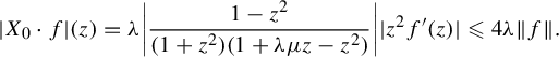
The argument is identical for $\mathrm {Re}(z)\leq 0$
on
$\mathrm {Re}(z)\leq 0$
on $V^{-}$
.
$V^{-}$
.
(3) Here, $f\in \mathcal {B}$
.
$f\in \mathcal {B}$
.
-
(a) On the disc
$\tfrac 14\mathbb {D}$
, we have
$|X_{0}\cdot f^{\pm }|\leq \tfrac 12$
so that
$\tfrac 12\leq |1+X_{0}\cdot f^{\pm }|\leq \tfrac 32$
: we can bound the magnitude of the sectorial vector field
$X^{\pm }=({1}/({1+X_{0}\cdot f}))X_{0}$
by
$$ \begin{align*} \bigg(\text{for all }|z|\leq\frac{1}{4}:\pm\mathrm{Re}(z)\geq0\bigg)\quad\frac{4\unicode{x3bb}|z|^{2}}{15}\leq {|\text{X}^{\pm}(\text{z})|\leq}\frac{20\unicode{x3bb}|z|^{2}}{3}. \end{align*} $$
-
(b) Invoking the same variational argument as in the proof of Lemma 5.1, if the a priori bound
holds, then the time-1 flow of
$$ \begin{align*} \frac{r}{1-({20\unicode{x3bb} r}/{3})} \leq\frac{1}{4} \end{align*} $$
$z\in r\mathbb {S}^{1}$
along
$X^{\pm }$
is well defined and lands in
$\tfrac 14\mathbb {D}$
. However, the condition is fulfilled for
$r:={3}/{16}$
since
${20\unicode{x3bb} r}/{3}={5\unicode{x3bb} }/{4}<{5}/{32}$
.
-
(c) Because
$\Delta $
is a symmetry of
$X^{\pm }$
, we have
$X^{\pm }\cdot \Delta =X^{\pm }\circ \Delta $
, that is, For
$$ \begin{align*} |\Delta'| =\frac{|X\circ\Delta|}{|X|}. \end{align*} $$
$|z|={3}/{16}$
, we obtain Continuing, we find


Consider now $\Delta _{1}$
and
$\Delta _{1}$
and $\Delta _{2}$
in normal form, being the respective time-1 map of
$\Delta _{2}$
in normal form, being the respective time-1 map of $X_{j}^{\pm }:=({1}/({1+X_{0}\cdot f_{j}^{\pm }}))X_{0}$
with
$X_{j}^{\pm }:=({1}/({1+X_{0}\cdot f_{j}^{\pm }}))X_{0}$
with $f_{j}\in \mathcal {B}$
for given
$f_{j}\in \mathcal {B}$
for given $0<\unicode{x3bb} <\min \{ {1}/{2|\mu |},\frac 18\} $
as in the proposition. Being given
$0<\unicode{x3bb} <\min \{ {1}/{2|\mu |},\frac 18\} $
as in the proposition. Being given $O=(O^{-},O^{+})$
, we introduce the slight abuse of notation:
$O=(O^{-},O^{+})$
, we introduce the slight abuse of notation:
and choose
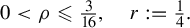 $$ \begin{align*} 0<\rho\leq\tfrac{3}{16},\quad r:=\tfrac{1}{4}. \end{align*} $$
For the sake of readibility, we drop the superscripts $\pm $
altogether.
$\pm $
altogether.
If $z_{1}$
,
$z_{1}$
, $z_{2}$
is the respective trajectory of
$z_{2}$
is the respective trajectory of $X_{1}$
,
$X_{1}$
, $X_{2}$
emanating from some common
$X_{2}$
emanating from some common $z\in \rho \overline {\mathbb {D}}$
, then
$z\in \rho \overline {\mathbb {D}}$
, then $\phi :=|z_{1}-z_{2}|^{2}$
solves
$\phi :=|z_{1}-z_{2}|^{2}$
solves
 $$ \begin{align*} \dot{\phi} =2\mathrm{Re}((X_{1}(z_{1})-X_{2}(z_{2}))\overline{z_{1}-z_{2}}),\quad \phi(0)=0. \end{align*} $$
Since $z_{1}(t),~z_{2}(t)\in r\mathbb {D}$
for all
$z_{1}(t),~z_{2}(t)\in r\mathbb {D}$
for all $t\in [0,1]$
, we have
$t\in [0,1]$
, we have
The proposition yields

and
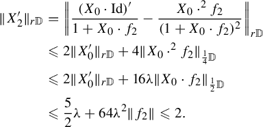
From a direct integration of
 $$ \begin{align*} (\text{for all }|t|\leq1)\quad\bigg|\frac{\dot{\phi}}{2\sqrt{\phi}(a+2\sqrt{\phi})}\bigg| \leq1, \end{align*} $$
we finally deduce the following estimate.
Lemma 6.2. We have
Assume now that ![]() and pick
and pick ![]() less than the least radius of convergence of
less than the least radius of convergence of ![]() , so that
, so that ![]() , and consider
, and consider
similarly as in Proposition 4.14. Invoking equation (4.6), we derive
that is,
provided $\unicode{x3bb}>0$
be small enough to ensure
$\unicode{x3bb}>0$
be small enough to ensure ![]() , say. By assumption, we have
, say. By assumption, we have $\mathfrak {m}_{\mu }\exp (2\pi -{1}/{\unicode{x3bb} })\leq {\rho }/{2}$
so that Cauchy’s formula applied on
$\mathfrak {m}_{\mu }\exp (2\pi -{1}/{\unicode{x3bb} })\leq {\rho }/{2}$
so that Cauchy’s formula applied on $\rho \mathbb {S}^{1}$
yields
$\rho \mathbb {S}^{1}$
yields
from which we deduce
We write $\Delta _{j}=\mathrm {Id}\exp \delta _{j}$
with
$\Delta _{j}=\mathrm {Id}\exp \delta _{j}$
with $\delta _{j}(0)=0$
which, thanks to Proposition 6.1(3)(c), satisfies
$\delta _{j}(0)=0$
which, thanks to Proposition 6.1(3)(c), satisfies ![]() . Because we iterate
. Because we iterate $\text {Synth}_{\unicode{x3bb} }$
, we lose no generality in assuming
$\text {Synth}_{\unicode{x3bb} }$
, we lose no generality in assuming ![]() as well. Supposing therefore
as well. Supposing therefore
 $$ \begin{align*} \frac{171}{\rho}{e}^{11}\mathfrak{m}_{\mu}\unicode{x3bb}^{4} \leq\frac{1}{44}, \end{align*} $$
we deduce for $|z|=\rho $
,
$|z|=\rho $
,

As a matter of consequence, we have
Now, we can choose the right constants in advance.
Corollary 6.3. Pick ![]() and
and $\rho :={3}/{16}$
; let
$\rho :={3}/{16}$
; let $\mathcal {B}_{11}$
be the ball
$\mathcal {B}_{11}$
be the ball ![]() . Define
. Define
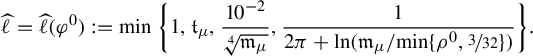
For any
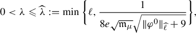
the partial map ![]()
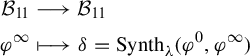
is a well-defined ${1}/{22}$
-Lipschitz map. Its unique fixed-point
${1}/{22}$
-Lipschitz map. Its unique fixed-point $\delta _{*}$
provides the sought fixed-point
$\delta _{*}$
provides the sought fixed-point $\Delta _{*}:=\mathrm {Id}\exp \delta _{*}$
of the parabolic renormalization.
$\Delta _{*}:=\mathrm {Id}\exp \delta _{*}$
of the parabolic renormalization.
6.2 Real synthesis
Let $\mu \in \mathbb {R}$
and
$\mu \in \mathbb {R}$
and ![]() be given such that condition
be given such that condition $(\square )$
holds:
$(\square )$
holds:
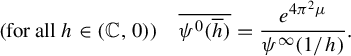
Expressed for the data ![]() , it becomes
, it becomes
Recall that $\Delta =\Phi _{X}^{1}$
, where
$\Delta =\Phi _{X}^{1}$
, where $X=({1}/({1+X_{0}\cdot f}))X_{0}$
and f is obtained as the limit of the iteration
$X=({1}/({1+X_{0}\cdot f}))X_{0}$
and f is obtained as the limit of the iteration $(f_{n})_{n}$
defined by
$(f_{n})_{n}$
defined by
as in Definition 4.13. We wish to prove that f is a real function by induction on n. This is clearly true for $n:=0$
and it is sufficient to prove that
$n:=0$
and it is sufficient to prove that $\Lambda _{f}$
is real.
$\Lambda _{f}$
is real.
Assume that $\overline {f_{n}(z)}=f_{n}(\overline {z})$
for every
$\overline {f_{n}(z)}=f_{n}(\overline {z})$
for every $z\in V$
(this identity is well defined because V is invariant by the complex conjugation). Because
$z\in V$
(this identity is well defined because V is invariant by the complex conjugation). Because $\overline {a}=b$
, we only need to check that
$\overline {a}=b$
, we only need to check that
where we have set
 $$ \begin{align*} H_{n}(\xi):=H_{f_{n}}^{+}(\xi) =H_{0}(\xi)\exp(2{i}\pi f_{n}^{+}(\xi)), \end{align*} $$
which in turn holds thanks to $(\widetilde {\square })$
whenever
$(\widetilde {\square })$
whenever $\overline {H_{n}(\overline {\xi })}={1}/{H_{n}(\xi )}$
. By the induction hypothesis, we can assert
$\overline {H_{n}(\overline {\xi })}={1}/{H_{n}(\xi )}$
. By the induction hypothesis, we can assert
 $$ \begin{align*} \overline{H_{n}(\overline{\xi})} =\overline{H_{0}(\overline{\xi})}\exp(-2{i}\pi f_{n}^{+}(\xi))=\frac{1}{H_{n}(\xi)} \end{align*} $$
since, according to equation (4.1):
 $$ \begin{align*} \overline{H_{0}(\overline{\xi})} =\exp\bigg(2{i}\pi\frac{1-\xi^{2}}{\unicode{x3bb}\xi}+2{i}\pi\mu\log\frac{1-\xi^{2}}{\unicode{x3bb}\xi}\bigg)=\frac{1}{H_{0}(\xi)}. \end{align*} $$
This completes the proof of the Real Synthesis Corollary.
Acknowledgments
I would like to express my greatest gratitude to my skilful colleague R. Schäfke, who introduced me to the joy of holomorphic fixed-point methods in dynamics. The author was partially supported by the bilateral Hubert–Curien Cogito grant 2021-22.


