A multiscale model for espresso brewing: Asymptotic analysis and numerical simulation

Abstract

We present a novel multiscale mathematical model of espresso brewing. The model captures liquid infiltration and flow through a packed bed of ground coffee, as well as coffee solubles transport (both in the grains and in the liquid) and solubles dissolution. During infiltration, a sharp interface separates the dry and wet regions of the bed. A matched asymptotic analysis (based on fast dissolution rates) reveals that the bed can be described by four asymptotic regions: a dry region yet to be infiltrated by the liquid, a region in which the liquid is saturated with solubles and very little dissolution occurs, a slender region in which solubles are rapidly extracted from the smallest grains, and region in which slower extraction occurs from larger grains. The position and extent of each of these regions move with time (one being an intrinsic moving internal boundary layer) making the asymptotic analysis intriguing in its own right. The analysis yields a reduced model that elucidates the rate-limiting physical processes. Numerical solutions of the reduced model are compared to those to the full model, demonstrating that the reduced model is both accurate and significantly cheaper to solve.

1 Introduction

Since coffee consumption was introduced to countries and regions with colder climates, it has become an important commodity with increasing demand and a major role in the economic stability of both producing and consuming countries [15]. In the UK alone, people drink approximately 98 million cups of coffee daily and demand continues to grow [4]. The growth of supply of coffee beans, however, is limited as coffee can only grow in very particular warm climates with some of the most popular coffee beans coming from high-altitude mountain farms. Driven in part by climate change, we may soon face a supply deficiency which motivates us to better understand coffee extraction and attempt to minimise waste.

One of the most popular coffee drinks is the espresso; the Specialty Coffee Association defined an espresso [41] as a 25 – 35 mL (ca. 20 – 30 g) beverage prepared from 7 – 9 g (or 14 – 18 g for a double) of ground coffee made with water heated to $92-95 ^\circ C$ , forced through the granular bed under 9 – 10 bar of static water pressure and a total flow time of 20 – 30 s. That being said, professional baristas often diverge from these guidelines considerably in order to produce stylised drinks and/or based on the coffee beans and roast. Espresso is the base for many coffee-based beverages, including latte, cappuccino and Americano, motivating us to focus on espresso brewing.

Multiple factors come together to determine the taste and quality of a beverage such as input dose (dry coffee mass), temperature, brew time, tamp pressure, water pressure, grind settings, basket size, etc. Even a small variation in any one of these can lead to fluctuations in the output beverage. Thus, a challenge for baristas has always been the consistency of espressos; drinks are challenging to reproduce and brewing the same recipe often results in variations of the taste. Flavour is a characteristic that is hard to quantify and measure (a task falling in the realm of sensory science); however, correlations have been observed between taste and more readily quantifiable measures. Professionals often refer to the so-called ‘brew chart’ that correlates the brew strength (mass concentration of dissolved coffee solids), or BS, with the extraction yield (EY) of a drink – the ratio of solvated coffee mass in the shot to the dry mass used for the shot. A coffee drink consists of over 1800 different chemicals [32] that are difficult to measure, so instead the coffee industry benchmarks shots in terms of the total amount of dissolved solids (TDS) which can in turn be used to calculate the EY.

In the past decade, the techniques of mathematical modelling have been applied to coffee brewing with the aim of understanding the physical processes in various coffee brewing apparatus and ultimately enabling predictive models which can complement experiments to optimise flavour and minimise waste. We note that other work has been done on the adjacent problem of coffee roasting, see e.g., Fadai et al. [10]. The problem is also of significant mathematical interest because it requires modelling of coupled physical processes (fluid flow, chemical dissolution, solute transport, etc.) across multiple scales (coffee cellular scale, grain scale and the bed scale). Early applications of mathematical modelling to coffee brewing focused on large-scale industrial extractors, namely so-called ‘diffusion batteries’. This work focused on optimising extraction behaviour, see [7, 38, 40]. More recently, research into modelling of coffee brewing includes a series of papers by Fasano and co-workers who developed general multiscale models of coffee extraction focusing mainly on the espresso brewing configuration [11–14]. Key publications building on this include the body of work by Moroney et al. [25, 27–29] who have presented a multi-scale dual-porosity model of coffee extraction derived using volume averaging for (i) a fixed coffee bed (e.g., drip-filter/espresso), and (ii) a well-mixed system (e.g., may be appropriate for French press/cafetiere brewing). Whilst these models have been somewhat successful in matching experimental measurements of BS and EY, the assumption that the microscopic transport is wholly limited by extraction at the surface and not transport in the bulk of particles means that the details of the microscale transport process within the coffee grains are lost.

In this work, we will show that transport in the larger grains is often rate-limiting for extraction, and its omission is therefore less than ideal. A similar approach, also using volume averaging, was applied by Sano et al. [36] who further simplified the model in [25] to reduce the number of parameters and improve its ease of use. Kuhn et al. [22] also applied an averaging procedure to arrive at a simplified macroscale model of solute transport. They applied their model to predict not only the total solubles concentration but also the concentration of individual coffee constituents, namely caffeine and trigonelline. After fitting, their model compared well to extraction data on these species for espresso shots. The works mentioned so far feature first-order expressions for the rate of transfer between the coffee grains and the intergranular liquid on the macroscale. If extraction of coffee is limited by intragranular diffusion (as expected for larger grains), these expressions cannot match the true shape of the extraction curve from different grains (albeit the discrepancy may be compensated for, at least partially, by tuning other model parameters appropriately). A more accurate description of extraction at the grain scale retains the microscale diffusion behaviour in the governing equations. This approach was taken in [24] who numerically solved a coupled microscale diffusion problem for coffee extraction from spherical coffee grains of different sizes with a macroscale advection problem describing one-dimensional coffee solubles transport in the intergranular pores of an espresso bed. A similar more general model for fluid and solute transport in an espresso bed was motivated from the full microscale equations using asymptotic homogenisation in [6]. Giacomini and co-workers [8, 18] did further work using the model of Cameron et al. [6] by solving it using a different numerical scheme, comparing results to a wide range of experimental conditions and extending the model to multiple dissolved coffee species which may interact through their concentrations. While it is clear there is a substantial literature on mathematical modelling of solute release from porous coffee beds, one aspect of the brewing process has been largely neglected to date: the initial transient behaviour which occurs when the invading water displaces the pervading gas in the initially dry porous bed prior to the full wetting of the bed. This will be a key focus of the current work. As we will show, capturing this initial behaviour is important because a substantial proportion of the extraction occurs in these early stages whilst the grains are soluble-rich.

The present work will build upon the multiscale model reported in [6] by including the initial period of liquid infiltrating the dry bed of ground particles, including both the inter- and intra-granular pore space. In espresso brewing, the initial infiltration period (i.e., until the first drip emerges from the portafilter) may take 5-10 s and therefore constitutes up to one-third of the total brewing time. Neglecting this phase, as previous work has done, requires ad hoc assumptions on initial conditions and therefore can be expected to limit model accuracy. In Section 2, we formulate the novel model. We non-dimensionalise the equations in Section 3 and identify the key dimensionless parameter (the ratio between the timescale for dissolution and that of wetting) that facilitates the asymptotic analysis that follows in Section 4. We will show that there are three asymptotic regions (plus a fourth dry region, the solution in which is trivial): a region in which the liquid is saturated with solubles and little dissolution occurs, another in which dissolution occurs relatively slowly from large grains, and a third narrow region between the two in which very rapid extraction occurs from small grains. Each of these regions moves with time. Systematically reducing the model using asymptotic analysis allows us to formulate a reduced model that is significantly easier to work with and interpret, and significantly faster to solve. In Section 5, we verify that the reduced model is accurate in appropriate parameter regimes and discuss some representative results. We draw our conclusions in Section 6.

2 Problem formulation

In this section, we formulate a model to describe extraction from a bed of porous, partially soluble coffee grains. We will be inspired by the multiple scales homogenisation results presented in [6] and model a bed with two disparate length scales, namely the size of the bed and the size of the grains (hereafter referred to as the microscale and the macroscale respectively). As is a central assumption in any multiple scales calculation, we assume that the coordinate systems pertaining to these two length scales are independent. This structure of multiscale model notably appears in the ubiquitous physics-based model for lithium-ion batteries, namely the Newman model [34], which was established in the mid-90s and has since been widely used to model real devices and compared to experimental data [44].

Initially, the bed is dry and water is injected at the bed inlet. Water enters the interstitial space between grains (intergranular pore space), while also being absorbed into the internal (intragranular) pore space contained in the cellular matrix of the coffee grains, see Figure 1. Once the grains are wet, extraction begins: solubles dissolve internally and are transported to the surface of the grains where they can enter the liquid in the intergranular pore space, then move through the liquid via a combination of diffusion and advection, and ultimately out of the bed and into the cup. In this work, wetting at the grain scale will be assumed to be instantaneous. This assumption is expected to be accurate when the timescale for grain wetting is much shorter than that for coffee solubles release and is made here in the absence of any clear experimental data in the literature that shows delayed wetting at the grain scale. In the following sections, we will formulate a system of partial differential equations describing (i) the flow of liquid through the bed, (ii) the transport of solubles in the intragranular pore space, (iii) the mass transfer for soluble material from the granular surfaces to the intergranular liquid and (iv) the transport of coffee solubles through the intergranular pore space.

2.1 Grain geometry

It is widely reported in the literature [21, 25, 35, 43] that ground coffee has a bi-modal particle size distribution. As such, grains are often divided into two groups, termed boulders and fines. Boulders (larger than 100 $\mu$ m in diameter) are shown to be porous, and their internal porosity, $\varphi _{lb}$ , varies with bean origin, pretreatment and roasting processes, typically in the range $35\%-55\%$ [37]. In our model, the porous volume in any particular boulder is assumed to be instantaneously filled with liquid when liquid arrives outside the grain. Fines (smaller than 100 $\mu$ m) are assumed to have an internal structure that cannot be accessed by water. Ground coffee particles come in a wide variety of irregular shapes but for simplicity, we will approximate both types of grains as spherical with radii $a_i^*$ , for $i=f,b$ denoting fines and boulders respectively and the superscript ‘ $*$ ’ is used to indicate dimensional quantities. We define the radial coordinate $0 \leq r_i^* \leq a_i^*$ to be the distance from the centre of a grain of type $i$ .

2.2 Bed geometry

Espresso is brewed in a cylindrical container of height $L^*$ and radius $R_0^*$ . It is assumed that the properties of the bed are homogeneous in any circular cross-section, the liquid is uniformly injected at the inlet and the drag caused by the cylinder walls is negligible. Thus, macroscopically, i.e., on the scale of the whole bed (much larger than individual grains), the model for flow and transport in the intergranular pore space is one-dimensional. Hence, it is sufficient to form one-dimensional equations on the macroscale and define the coffee bed to lie in $0\leq z^* \leq L^*$ (see Figure 1). The inlet is located at $z^*=0$ and the outlet at $z^*=L^*$ .

The entirety of the coffee bed volume comprises of spherical grains and the space between them. The ratio of the total volume of grains to the bed volume is given by $\phi _s$ . The space between the grains (intergranular pore space) is initially occupied by air and is subsequently filled with liquid and has a volume fraction of the entire bed $\phi _l$ . The grain volume consists of the two size classes of grains, namely fines and boulders and their volume fractions (measured with respect to the whole bed) are $\phi _f$ and $\phi _b$ , respectively. Since the bed is homogeneous, these volume fractions are constant in any circular cross-section of the bed. Thus,

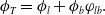
(1) \begin{align} \phi _{l} + \phi _s &= 1, & \phi _{s} & = \phi _{f} + \phi _{b}. \end{align}

The boulders are themselves porous, and their internal pores are accessible by liquid. Before a boulder comes in contact with liquid, its pore space is filled with air which (we assume) is instantaneously replaced by liquid on wetting. The fraction of the boulders’ volume (measured with respect to the boulders’ volume) accessible by liquid is taken to be $\varphi _{lb}$ , introduced above. We note that grains may swell when in contact with the liquid and increase their volume; however, there is disagreement in the literature over whether swelling is negligible [23] or significant ( $\sim 15 \%$ ) [20]. Thus, due to the lack of consensus and in the interest of simplicity, we will not consider this phenomenon. Therefore, the total porosity $\phi _T$ of the bed is the sum of the intergranular pore space and the pore space within the boulders, that is

(2) \begin{equation} \phi _{T} = \phi _{l} + \phi _{b}\varphi _{lb}. \end{equation}

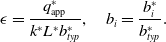
We model the transfer of solubles from grains to liquid as taking place on the spherical outer surface of the grains, i.e., any dissolution of solubles that occurs within the pore space of infiltrated boulders is not included as grain-to-liquid transfer. Equations for the rate of transport within grains (in the case of boulders this includes both the internal solid and liquid phases) and across the grain/liquid interface (the spherical outer surface of the grains) shall be formulated shortly. We therefore introduce the reactive spherical outer surface area of the grains (on which solubles can be transferred from grains into liquid) as the Brunauer-Emmett-Teller surface area, $b_i^*$ , defined to be the reactive surface area of grains of species $i$ per unit volume of bed. These are given by

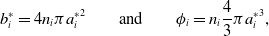(3) \begin{align} b_i^* = 4 n_i \pi {a_i^*}^2 \qquad \text{and} \qquad \phi _i = n_i \frac {4}{3} \pi {a_i^*}^3, \end{align}

where $n_i$ is the number of grains of type $i$ per unit volume of the bed. Hence, on eliminating $n_i$ between the two expressions in (3) we arrive at

(4) \begin{align} b_i^* = \frac {3 \phi _i}{a_i^*}. \end{align}

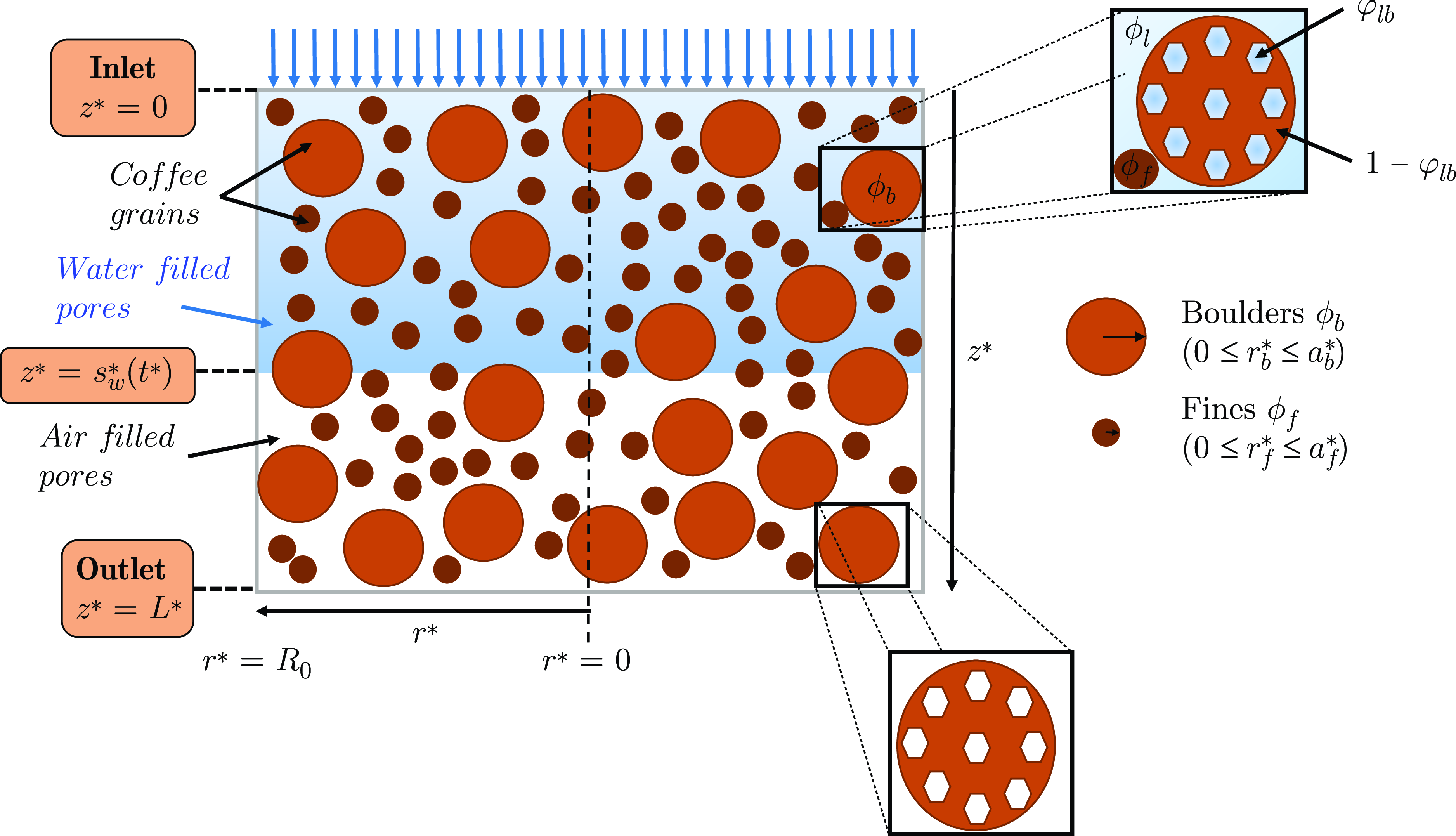
Figure 1. A cartoon of the bed geometry. The liquid is injected at the inlet, located at $z^* = 0$ and exits the bed through the outlet at $z^* = L^*$ . During infiltration, the wetting front is located at $z^* = s_w^*(t^*)$ . The local volume fractions of the liquid, fines and boulders are given by $\phi _l, \phi _f$ and $\phi _b$ respectively. The volume fraction of pore space within a boulder is given by $\varphi _{lb}$ .

2.3 Liquid flow

We model the flow in the intergranular pore space using Darcy’s law with the incompressibility condition [1, 33]. While the density of the liquid varies only slightly with soluble coffee content, the viscosity may be significantly higher than that of pure water at higher concentrations [31]. Nonetheless, in the interests of simplicity, we elect to follow Moroney et al. [25] and adopt a constant density and viscosity approximation. The choice of boundary condition at the inlet depends upon the espresso machine of interest and in particular how its pump operates; most commonly this can apply either a fixed flow rate or a fixed pressure. Both situations are readily modelled, but here we choose to focus primarily on the fixed flow case for convenience. Readers interested in the fixed pressure case are referred to the supplementary material where this problem is presented.

On denoting the volumetric flux/Darcy flux (measured in units of m/s) by $q^*$ , incompressibility amounts to the statement that $\partial q^* / \partial z^* =0$ . On supplementing this with a fixed flow rate boundary condition at the inlet, we immediately learn that throughout the wet region we have

(5) \begin{align} q^*|_{z^*=0} = q^*_{\text{app}}, \qquad \text{and thus,} \qquad q^* = q^*_{\text{app}}. \end{align}

Provided that the shot is brewed properly (no channelling or clogging), the interface between the wet and dry parts of the bed appears to be sharp, as can be seen in experiments when espresso is brewed in a transparent portafilter [17]. The physics of the wetting process involves a complex interplay of the applied pressure, surface tension, capillary forces, swelling of the coffee cellular matrix, release of trapped gases (mainly carbon dioxide [7, 39]) and potentially the nature of the dissolved solids in the water phase [9]. Here, we opt to avoid having to treat these phenomena and instead will make the assumption that the infiltration of the water into the intergranular pore space is described by Darcy’s law, as above, and that infiltration into the intragranular pore space is instantaneous on contact with water. Once water has entered the intragranular pore space, we will assume that it can no longer flow. On denoting the location of the wetting interface by $s_w^*(t^*)$ we have

(6) \begin{align} \phi _T \frac {ds_w^*}{dt^*} = q^*|_{z^*=s_w^*(t^*)} \end{align}

which states that the volumetric flux must be equal to the volume of pore space swept through by the wetting interface per unit time. We supplement this ordinary differential equation (ODE) for $s_w^*$ with the initial condition

(7) \begin{align} s_w^*|_{t^*=0} = 0 \end{align}

and note that when the waterfront arrives at the outlet of the machine $z^* = L^*$ , there is no longer a need to track the position of the interface. Solving (6) with (5) and (7) yields

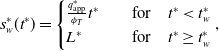(8) \begin{align} s_w^*(t^*) = \begin{cases} \frac {q_{\text{app}}^*}{\phi _{T}}t^* \quad &\text{for} \quad t^*\lt t_w^* \\ L^* \quad &\text{for} \quad t^* \geq t_w^* \end{cases}, \end{align}

such that at a time $t^*=t_{w}^*= \phi _T L^* / q_{\text{app}}^*$ the whole bed is saturated with water.

2.4 Transport in the intergranular pore space

We will model the change in concentration of coffee solubles in the three distinct volumes, namely the intergranular pore space and the space occupied by fines and boulders. It has been assumed that the macroscopic variables are one-dimensional, depending only on depth in the bed ( $z^*$ ). In the subsequent subsection, we will further assume that the microscale transport ( i.e., that of solubles in the interior of the grains) is also one-dimensional and depends only on radial distance from the centre of a grain $r^*$ . The model that we are in process of forming can aptly be termed a pseudo 2D model, similar to the Newman model [34] which is the standard electrochemical model used to describe the operation of lithium-ion batteries. Thus, the model variable denoting the concentration of solubles in the liquid, $c_l^*=c_l^*(z^*,t^*)$ , is defined in the wet part of the bed $(0\leq z^*\leq s_w^*)$ and measured as the mass of solubles per unit volume of wet intergranular pore space. The concentration within the boulders is denoted by $c_b^*=c_b^*(r_b^*,z^*,t^*)$ and that in fines by $c_f^*=c_f^*(r_f^*,z^*,t^*)$ ; both of which are defined within the respective grains $(0\leq r_i^*\leq a_i^*) \times (0\leq z^*\leq L^*)$ for $i=b,f$ and measured per unit volume of grain. In the case of boulders, and consistent with previous assumptions, this grain volume is taken to include both the internal solid and liquid phases. We note that although the concentrations in the fines and boulders depend on two spatial variables, $r^*$ and $z^*$ , it is apposite to say that the microscopic equations are one-dimensional because (as we will see shortly) only derivatives with respect to $r^*$ appear in the governing PDEs, see (13)-(14).

We now formulate the equations governing the transport in the intergranular pore space, and those governing the transport in the grains will be treated in Section 2.5. The coffee solubles migrate through the liquid via a combination of diffusion and advection by the flow therefore, at macroscopic length scales, we have

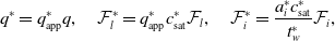
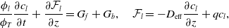
(9) \begin{align} \phi _l \frac {\partial c_l^*}{\partial t^*} + \frac {\partial {\mathcal F}_l^*}{\partial z^*} = b_{f}^* G_f^* + b_{b}^* G_b^*, \quad {\mathcal F}_l^* = - D_{\text{eff}}^* \frac {\partial c_l^*}{\partial z^*} + q^* c_l^*, \end{align}

where $c_l^*$ is the mass concentration of solubles in the liquid, ${\mathcal F}_l^*$ is the flux of these solubles, $D_{\text{eff}}^*$ is the effective macroscopic diffusivity and $G_i^*$ are the mass fluxes of solubles exiting the grains and entering the water, measured on the surfaces of the fines ( $i=f$ ) and boulders ( $i=b$ ). The effective macroscopic diffusivity $D_{\text{eff}}^*$ accounts for both diffusion and also mechanical (hydraulic) dispersion, which arises from solute mixing due to microscale variations in the flow, at macroscopic scales. Ideally, this effective transport property should be computed via a suitable homogenisation procedure, see e.g., [16]. Alternatively one could approximate its value using, e.g., Bruggeman’s relation [5].

The physically correct condition to apply at the inlet is that of continuity of flux. However, we do not wish to expand the model to involve the flow of water upstream of the inlet. To this end, and with foresight that parameters estimates will soon tell us that advective effects are dominant over diffusive ones, see Section 3, we choose to say impose that the liquid entering the bed is solubles-free and therefore we impose

(10) \begin{align} c_l^* |_{z^*=0} =0. \end{align}

An alternative, that also avoids needing to include a model for the flow upstream of the inlet, would be to require that the flux of solubles at the inlet is zero, i.e., ${\mathcal F}_l^*|_{z^*=0}=0$ ; however in the relevant scenario, where advective effects dominate diffusive ones, this collapses to (10). At the wetting front, we enforce conservation of solubles accounting for the movement of the front and allowing solubles to move from the liquid in the intergranular pore space and into the pore space inside the boulders. To formulate this condition, we apply a ‘Gaussian pillbox’ [19] argument; details are given in the supplementary material. The model doesn’t capture the flow after it leaves the bed, therefore we require a boundary condition at the outlet $z^* = L^*$ . We choose to impose zero diffusive flux at the outlet; however, this boundary condition is passive as it has no effect on the asymptotic analysis that follows. The set of boundary conditions supplementing (9) is as follows:

(11) \begin{align} -\frac {d s_w^*}{dt^*} \phi _l c_l^*|_{z^*=s_w(t)} + {\mathcal F}_l^*|_{z^*=s_w^*(t^*)} = \frac {d s_w^*}{dt^*} \phi _b \varphi _{lb} c_l^* |_{z = s_w^*(t^*)} \, \, \text{for} \, \, t^*\lt t_w^*, \end{align}

(12) \begin{align} \frac {\partial c_l^*}{\partial z^*}|_{z^*=L^*} = 0 \, \, \text{for} \, \, t^*\geq t_w^*. \end{align}

2.5 Transport in the intragranular pore space (coffee grains)

We follow previous studies [6, 26] and model the transport of solubles in the grains by Fickian diffusion. Each grain contains a concentration of soluble coffee $c_f^*$ or $c_b^*$ for fines and boulders, respectively. Since boulders have an internal pore fraction $\varphi _{lb}$ , the concentration $c_b^*$ should be understood as the mass of solubles per unit volume within the boulder including both the solid and liquid phases, by contrast, that in fines, $c_f^*$ , is the mass of solubles per unit volume of solid (the fines are assumed to have zero internal porosity). When the grains become wet, the solubles migrate from the centre towards the surface of the grain and once they are at the surface, they are transported to the surrounding liquid at a rate $G_i^*$ , to be defined shortly. The multiscale nature of the model requires that, at each location in macroscopic space $z^*$ , there is a microscopic coordinate $r_i^*$ denoting the distance from the centre of the grains. The concentration of coffee solubles is assumed to be spherically symmetric and that solubles become immediately mobile after wetting. The latter assumes that dissolution of solid coffee within the grains takes place on a much faster timescale than diffusion of dissolved coffee out of the grains. Thus

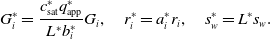
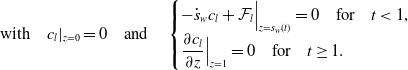
(13) \begin{align} \frac {\partial c_{i}^*}{\partial t^*} + \frac {1}{r_i^{*2}} \frac {\partial }{\partial r_i^*} \left ( r_i^{*2} {\mathcal F}_i^* \right )=0, \quad {\mathcal F}_i^* = - D_{si}^* \frac {\partial c_i^*}{\partial r_i^*}, \quad \text{for} \quad i=b,f, \end{align}

with boundary conditions

(14) \begin{align} {\mathcal F}_i^* \Big {|}_{r_i^*=0} = 0, \qquad {\mathcal F}_i^* \Big {|}_{r_i^*=a_i^*} = G_i^*, \end{align}

where $D_{si}^*$ is the diffusivity of solubles within the grains for $i = b,f$ . In light of our previous assumptions, these material properties should strictly be thought of as effective diffusivities that characterise the rate of transport through the grains‘ internal multiphase structure. Roasted coffee beans can be considered to consist of porosity made up of larger spherical pores (cell lumina with radii of approximately $2\times 10^{-5}$ m, connected by nanoscale pores in the cell walls (the walls have thicknesses of approximately $10^{-5}$ m. The internal structure of the two grain types being different, e.g., in contrast to the fines the boulders have much more significant internal pore space, therefore likely means that $D_{sb}^*$ and $D_{sf}^*$ differ.¹ Despite this, and in order to simplify the subsequent analysis, we will later assume they may be taken to be equal as a first approximation.

The initial concentration of solubles coffee per unit volume of grain, in fines and boulders (prior to wetting) is

(15) \begin{align} c_i^*|_{t^*=0} = c_{i,\text{init}}^*. \end{align}

In accordance with our previous assumptions, in the case of boulders, this is the be understood as the concentration per unit volume of both internal solid and pore space. Thus, the maximum mass of solubles that can be extracted from a given grain is $4\pi a_i^3/3$ for $i=b,f$ . When the wetting front moves through the bed, the liquid instantaneously fills the internal pores of the boulders. The infiltrating liquid may well be carrying solubles and therefore, immediately after the boulder is wet, the concentration of solubles in the boulder (measured with respect to both solid and now wet pore space) is

(16) \begin{align} c_b^*|_{z^*=s_w^*(t^*)}= c_{b,\text{init}}^* + c_l^*|_{z^*=s_w^*(t^*)}\varphi _{lb}. \end{align}

Thus, it is conceivable that shortly after wetting the concentration in the boulders is higher than the saturation concentration, i.e., $c_b^* \gt c_{\text{sat}}^*$ . Should this occur, in reality we would expect that solubles in the solid phase of the boulders would remain in solid immobile form until the local concentration within the pore space of the boulder drops sufficiently to allow internal dissolution to take place. We have adopted an effective/homogenised description of the internals of the boulders and assumed that dissolution of the solid phase solubles is always instantaneous; therefore, our model is incapable of capturing this phenomena systematically. Alleviation of this shortcoming is left open for future investigation but interested readers are directed to [30] which may provide a starting point for the remedy.

2.6 Mass transfer between grains and liquid in the wet region

Selecting a suitable extraction rate is non-trivial; however, we will assume that a sensible rate should have the following properties: (i) there is no transfer when the liquid immediately outside the grain is saturated, or when the concentrations of the liquid immediately outside is equal to that on its surface; (ii) mass transfer from regions with low concentration to regions with high concentrations is higher than regions with similar concentrations. With these in mind, we define an extraction rate similar to Cameron et al. [6] and say that

(17) \begin{align} G_i^{*} = k^*\begin{cases} c^*_{\text{sat}}-c^*_{l} \quad \text{if} \quad c_{i}^*|_{r^*_i=a^*_i} \geq c^*_{\text{sat}} \\ c^*_{i}|_{r^*_i=a^*_i}-c^*_{l} \quad \text{if} \quad c^*_{i}|_{r^*_i=a^*_i} \lt c^*_{\text{sat}} \end{cases} \end{align}

where $k^*$ is the mass transfer rate constant that has units $ \text{m s}^{-1}$ and $c^*_{\text{sat}}$ is the saturation concentration of solubles in the liquid. We emphasise that more sophisticated choices for the rate of mass transfer are certainly possible. For example, if data were to become available that shed light on the equilibrium relationship between the concentration of coffee in the grains and that in the liquid one could include then include and select an appropriate value for a partition coefficient [2, 24, 35]. In fact, there are good reasons to expect that this may be warranted. First, the concentrations in the different phases (boulders, fines and liquid) are measured with respect to different reference volumes: in the grains, it is measured per unit volume of grain including both intragranular pores and the internal solid structure whereas in the liquid it is per unit volume of liquid only. Thus, these may differ from the true local concentrations within the grain’s internal pores, which is what we might expect to be in equilibrium with the concentration in the liquid. Second, chemical binding and interactions of different coffee molecules with the intragranular matrix may also result in alterations to the equilibrium concentrations thereby warranting the inclusion of a partition coefficient. This being said, owing to the lack of requisite data, we follow [24] and assume a partition coefficient of unity for both grain species. Before moving on, we point out that the inclusion of a partition coefficient makes little difference to the overall structure of ensuing analysis and therefore does not hamper our central aim of elucidating the mathematical structure of the problem. More details on the partition coefficient and attempts to measure it can be found in [35].

2.7 Does saturation occur?

As we will demonstrate, it is possible to distinguish two varieties of espresso recipe, namely those that give rise to extractions in which the liquid that initially leaves the bed is so concentrated that it is fully saturated vs. those in which it is not. We have conducted experiments in which the first drips of liquid from a café-style espresso recipe are segregated from the remainder of the shot. The concentration of solubles in these initial drips appears to be fixed, independent of the details of the recipe, therefore suggesting that we have reached a maximum obtainable concentration which we expect to be the saturation limit of the water. More details on these experiments will be given in a forthcoming article. Whether saturation occurs is primarily determined by a competition between the rate of extraction from the fines (significantly faster than that from boulders owing to the size disparity between the two grain types) and the flow rate. When extraction from fines is fast compared to the flow rate, a saturated layer will form immediately above the wetting front because solubles are extracted from fines faster than they are transported away from the wetting front. This being said, fast transport within fines alone is not sufficient to form this saturated layer. In addition, fines must contain enough solubles (per unit volume of bed, $c_{f,\text{init}} \phi _f$ ) to saturate the surrounding liquid. Conversely, when extraction from fines is relatively slower and/or there are less solubles in the fines then saturation does not occur. Later in this work, in particular see (74) and the discussion shortly thereafter, we will be able to be more precise about demarcating these two regimes, however, for the time being, it is sufficient to note that for relevant parameter values, experimental evidence suggests that a saturated layer does form. As such, we shall, in the body of this paper present the analysis of regime in which a saturated layer forms; likewise is done for the case of no saturation in the supplementary material.

3 Non-dimensionalisation

We choose to scale time with the wetting time, $t_w^*$ , see (8) and the discussion immediately thereafter. We scale the vertical coordinate $z^*$ and the position of the front with the depth of the bed $L^*$ and radial position within grains with the radii of each grain type $a_i$ . The Darcy flux is scaled with that applied at the inlet $q_{\text{app}}$ . We scale all concentrations with the saturation concentration of the liquid, $c_{\text{sat}}^*$ . Equation (9) suggests that the flux of coffee solubles in the liquid $\mathcal{F}_l^*$ can be scaled either by the diffusion or advection term. A crude comparison of the sizes of these two flux components indicates that the advective flux will be dominant (this conclusion is confirmed by the experiments carried out in [6]), and so we scale $\mathcal{F}_l^*$ accordingly. The scalings for the fluxes inside the grains $\mathcal{F}_i$ are chosen in order to balance the terms in (13). Similarly, we chose a suitable scaling for the dissolution rates $G_i$ , where we define $b_{typ}^*$ as the arithmetic average of $b_b^*$ and $b_f^*$ . In summary, we set

(18) \begin{align} z^* = L^* z, \quad t^* = t_w^* t, \quad c_l^* = c_{\text{sat}}^* c_l, \quad c_{i}^* = c_{\text{sat}}^* c_{i}, \end{align}

(19) \begin{align} q^* = q^*_{\text{app}} q, \quad {\mathcal F}_l^* = q_{\text{app}}^* c_{\text{sat}}^* {\mathcal F}_l,\quad {\mathcal F}_i^* = \frac {a_{i}^* c_{\text{sat}}^*}{t_w^*} {\mathcal F}_i, \end{align}

(20) \begin{align} \quad G_i^* = {\frac {c_{\text{sat}}^* q_{\text{app}}^*}{L^* b_{i}^*}}G_i,\quad r_i^* = a_i^* r_i, \quad s^*_{w} = L^*s_w. \end{align}

Applying these scalings introduces the following dimensionless parameters

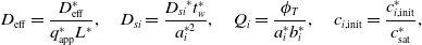(21) \begin{align} D_{\text{eff}} = \frac {D_{\text{eff}}^*}{q^*_{\text{app}} L^{*}}, \quad D_{si} = \frac {{D_{si}}^* t_w^*}{a_i^{*2}}, \quad Q_i = {\frac {\phi _T}{a_i^* b_{i}^* }},\quad c_{i,\text{init}} = \frac {c_{i,\text{init}}^*}{c_{\text{sat}}^*}, \end{align}

(22) \begin{align} \epsilon = \frac {q_{\text{app}}^*}{k^* L^* b_{typ}^*}, \quad b_{i} = \frac {b^*_{i}}{b^*_{typ}}. \end{align}

Of those dimensionless parameters whose interpretation is not self-evident from their definition, $D_{\text{eff}}$ can be understood as the ratio of the timescale for advection to that of diffusion of solubles in the liquid, $D_{si}$ as the ratio of the timescale of wetting to that of transport inside the grains, $Q_i$ as the ratio between the flux on the surface of the grain to the diffusive flux inside it, and $\epsilon$ as the ratio between the timescale for soluble transport through the surfaces of the grains and that for wetting. Application of the scalings (18)-(20) to the equations (5)-(17) yields the following dimensionless model

(23) \begin{align} \frac {\phi _l}{\phi _T} \frac {\partial c_l}{\partial t} + \frac {\partial {\mathcal F}_l}{\partial z} = {G_f + {G}_b}, \quad {\mathcal F}_l = - D_{\text{eff}} \frac {\partial c_l}{\partial z} + q c_l, \end{align}

(24) \begin{align} \mbox{with} \quad {c}_l {|}_{z=0} = 0 \quad \mbox{and} \quad \begin{cases} \displaystyle - \dot {s}_w c_l + {\mathcal F}_l \Big {|}_{z=s_w(t)} =0 \quad \mbox{for} \quad t\lt 1,\\ \displaystyle \frac {\partial c_l}{\partial z}\Big {|}_{z=1}=0 \quad \mbox{for} \quad t \geq 1. \end{cases} \end{align}

The dimensionless equations for the coffee grains are

(25) \begin{align} \frac {\partial c_{i}}{\partial t} + \frac {1}{r_i^{2}} \frac {\partial }{\partial r_i} \left ( r_i^{2}{\mathcal F}_i \right )=0,\quad {\mathcal F}_i = - D_{si} \frac {\partial c_i}{\partial r_i}, \quad \text{for} \quad i=b,f, \\[-12pt] \nonumber \end{align}

(26) \begin{align} \mbox{with} \quad {\mathcal F}_i \Big {|}_{r_i=0} = 0 \quad \mbox{and} \quad {\mathcal F}_i \Big {|}_{r_i=1} = {Q}_iG_i. \\[6pt] \nonumber \end{align}

The surface fluxes are given by

(27) \begin{align} G_i = \frac {{b_i}}{\epsilon }\begin{cases} 0 \quad \text{if} \quad z\gt s_w(t) \\ 1-c_{l} \quad \text{if} \quad c_{i}|_{r_i=1} \geq 1 \\ c_{i}|_{r_i=1}-c_{l} \quad \text{if} \quad c_{i}|_{r_i=1} \lt 1 \end{cases} \end{align}

The condition at the front is given by

(28) \begin{align} c_b|_{z=s_w(t)}= c_{b,\text{init}} + c_l|_{z=s_w(t)}\varphi _{lb}, \qquad c_f|_{z=s_w(t)}= c_{f,\text{init}}. \end{align}

The flow rate and position of the wetting front are given by

(29) \begin{align} q(z,t) = 1, \quad s_w(t) = \begin{cases} t \quad \text{for} \quad t \leq 1, \\ 1 \quad \text{for} \quad t \gt 1. \end{cases} \end{align}

Equations (23)-(29) comprise the dimensionless model, the analysis of which we now turn our attention to.

3.1 Parameter estimates

The asymptotic analysis that follows requires estimates of the sizes of the dimensionless parameters. Currently, as far as we are aware, there is no complete set of parameters for espresso brewing. In an attempt to formulate such a set, we combine the estimates presented in [6, 25, 26, 32, 42].

The parameters $Q_i$ , $c_{i,\text{init}}$ , $b_i$ depend simply on the particle size distribution and bed packing. They are calculated based on estimates of $a_i^*$ in [25, 26] listed in Table 1, and would change slightly based on bed packing and the grind setting determining the size distributions of grains. The remaining parameters $D_{\text{eff}}$ , $D_{si}$ and $\epsilon$ depend on the diffusivities as well as the fluid velocity $q_{\text{app}}^*$ and the bed height $L^*$ and are comparable to the estimates given in [6]. In the absence of detailed experimental data, we shall now assume that the diffusivities in the boulders and fines are equal despite there being reasons to believe that this may not be the case; see the discussion under (14). Before moving on to the asymptotic analysis we point out that despite the naivety of assuming that the diffusivities in the boulders and fines are equal, there is little to no impact on the reduced model that we ultimately derive. In what follows we will examine the asymptotic limit that $D_{sf} \to \infty$ . As an upshot, the exact value of the diffusivity in the fines does not appear at leading order, and therefore our reduced model is insensitive to its value. Thus, the ensuing analysis holds provided future evidence does not indicate that the diffusivities change markedly from the estimates that we use here.

Table 1. Typical model parameter values. Those marked with superscript 1 are fitted to data, those with superscript 2 are available or can be estimated from the literature [6, 25, 26, 32, 42], and those marked with 3 are directly available from the experiment. Parameters marked with both superscripts 1 and 2 are fitted but their values are comparable to those available in the literature. We note that the diffusivities $D_{sf}^*,D_{sb}^*$ in the two grain species may differ due to their internal structure; however in the absence of data on those values, we use the same estimate

4 Asymptotic analysis

The estimates summarised in Table 2 indicate that

(30) \begin{align} D_{sb} = O(1), \quad D_{\text{eff}} = O(\epsilon ), \quad D_{sf} = O(\epsilon ^{-1/2}) \quad \mbox{where} \quad b_b= O(\epsilon ^{1/2}). \end{align}

The large values of $b_i/\epsilon$ , and the manner in which these ratios appear in (27), lead us to expect that large portions of the bed will be close to a state of quasi-equilibria in which either the liquid is saturated, or in which the concentration on the surface of the grains matches that in the surrounding liquid. The analysis presented in this section will exploit the smallness of $\epsilon$ by considering asymptotic solutions in the limit $\epsilon \to 0$ . The small value of $D_{\text{eff}}= O(\epsilon )$ indicates that throughout most of the bed transport by convection in the liquid dominates that by diffusion, retrospectively justifying our discussion in Section 2.7. The dimensionless diffusivity in the fines is large, which suggests that transport within fines is very rapid. The size of the dimensionless diffusivity in the boulders is taken to be $O(1)$ so that transport in the boulders occurs on a similar timescale to that of the infiltration. We note that one might be tempted to say that $D_{sb}=O(\epsilon )$ however, doing so would necessitate a temporal rescaling (to longer times) in order to understand how the boulders contribute to extraction which would complicate the analysis below. Besides, the case $D_{sb}=O(1)$ is a distinguished limit of the problem so that nothing is lost taking this to be the case for the purposes of the asymptotic analysis and then retrospectively allowing $D_{sb}$ to be small.

Table 2. Dimensionless parameters

We introduce the following scaled diffusivities

(31) \begin{align} D_{\text{eff}} = \epsilon \hat {D}_{\text{eff}}, \quad D_{sf} = \frac {\hat {D}_{sf}}{\epsilon }, \quad {b_b = {\epsilon ^{1/2}}{\hat {b}_b}} \end{align}

so that the hatted parameters are $O(1)$ .

4.1 Outline of the asymptotic analysis

For $t=O(1)$ the asymptotic structure of the solution, in the limit that $\epsilon \rightarrow 0$ , separates into three regions as shown in Figure 2. In Section 4.2, we analyse region (iii), adjacent to the wetting front, and in which the quasi-equilibrium for a saturated liquid pertains. Thus, in region (iii) there is little extraction and the solution structure is particularly simple. In Section 4.3, we examine region (ii), a narrow region separating regions (i) and (iii), in which the fines undergo rapid extraction, thereby allowing the concentration in the liquid to change markedly. Region (i), adjacent to the inlet, is the subject of Section 4.4. Here, the concentrations at the surfaces of the grains (of both types) and in the liquid are in a quasi-equilibrium. The boulders and fines undergo slow extraction leading to a concentration profile in the liquid that slowly increases with depth into the bed. In Section 4.5, we carry out the asymptotic matching required to tie all three regions together thereby closing the problem. A noteworthy feature of the analysis that follows is that the position of region (ii) cannot be determined in advance; instead must be determined as part of the solution to the problem. Thus, region (ii) can aptly be termed an intrinsic moving internal boundary, and the mathematics required to resolve this is interesting in and of itself.

For short times of $t=O(\epsilon )$ , before the saturated layer has formed the asymptotic structure is made up of only a single narrow spatial region. This single region is of width $O(\epsilon )$ and is located adjacent to the inlet. Here, the fines rapidly dissolve in order to boost the concentration in the incoming water to saturation. We shall not tackle this short time problem because our primary interest is predicting the concentration at the exit of the bed. The error engendered in omitting to analyse and include this short time problem (which would alter the ‘initial conditions’ for the $t=O(1)$ problem that is the focus of the remainder of this section) is small in the sense that it makes only an $O(\epsilon )$ difference to the prediction of the outlet concentration.

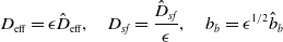
Figure 2. Schematics to illustrate the asymptotic structure of the problem. The left panel shows a snapshot of the different regions of the bed arising in the asymptotic analysis along with the moving boundaries $s_d(t)$ and $s_{w}(t)$ . The right panel shows the location of these moving boundaries evolving in the $z$ – $t$ plane. The wetting front, $s_w(t)$ , is represented by the solid black line. Region (iii) is located adjacent to the wetting front, region (i) is adjacent to the inlet. The saturation interface represented by the solid blue line and located at $z = s_d(t)$ , is surrounded by a narrow region (ii).

4.2 Region (iii): saturated liquid region

This region is located immediately behind the wetting front at $z=s_w(t)$ . The liquid is close to its saturation concentration and hence dissolution rates are almost zero. Grains in this region have not yet been in contact with unsaturated water and therefore will remain close to their initial concentration, with the boulder’s internal solubles concentration having been boosted by the infiltration of the saturated liquid. We seek an asymptotic solution in which all dependent variables are expanded in a regular asymptotic series in small $\epsilon$ as follows

(32) \begin{align} c_{l} = c_{l,0}^{\text{(iii)}}+ {o(1)}, \quad {c_{f}} = {c^{\text{(iii)}}_{f,0}}+ {o(1)}, \quad c_{b} = c_{b,0}^{\text{(iii)}} + {o(1)}, \end{align}

(33) \begin{align} {\mathcal F}_{l} = {\mathcal F}_{l,0}^{\text{(iii)}} + {o(1)}, \quad {\mathcal F}_{f} = {\mathcal F}_{f,0}^{\text{(iii)}} + {o(1)}, \quad {\mathcal F}_{b} = {\mathcal F}_{b,0}^{\text{(iii)}} + {o(1)}, \end{align}

(34) \begin{align} {G_{f}= G_{f,0}^{\text{(iii)}}+ {o(1)}, \quad G_{b}= G_{b,0}^{\text{(iii)}}+ {o(1)}}. \end{align}

In what follows we seek only the lowest-order terms, and thus, the size of the corrections is of secondary interest. Inserting these expansions in the definition of the reaction rates (27) and balancing leading order terms asserts that

(35) \begin{align} c_{l,0}^{\text{(iii)}} = 1, \end{align}

provided that $c_{f,0}^{\text{(iii)}}|_{r_f=1} \gt 1$ and $c_{b,0}^{\text{(iii)}}|_{r_b=1} \gt 1$ , which as we will show is typical in this region for our parameter set. The other possible balances $c_{f,0}^{\text{(iii)}}|_{r_f=1}=c_{l,0}^{\text{(iii)}}$ and $c_{b,0}^{\text{(iii)}}|_{r_b=1}=c_{l,0}^{\text{(iii)}}$ are rejected on the basis that the fines within region (iii) are yet to come into contact with liquid that is not saturated and therefore internal concentration remains at its initial value and boulders are topped up with saturated liquid. This result (35) also follows from the solution of (25) after inserting the expansions (32)-(34) and balancing leading order terms,

(36) \begin{align} c_{f,0}^{\text{(iii)}}= c_{f,\text{init}}, \quad {\mathcal F}_{f,0}^{\text{(iii)}} = 0. \end{align}

It follows from (28) that the boulders which have just been infiltrated with water, at $z=s_w(t)$ , have an internal concentration $c_{b,0}^{\text{(iii)}}|_{z=s_w(t)} = c_{b,\text{init}} + \varphi _{lb}\gt 1$ for a typical choice of parameters. Thus, since the boulders within region (iii) have also yet to come into contact with unsaturated water, and their internal concentration is larger than the saturation concentration of water, no mass transfer occurs at their surfaces and hence

(37) \begin{align} c_{b,0}^{\text{(iii)}} = c_{b,\text{init}} + \varphi _{lb}, \quad {\mathcal F}_{b,0}^{\text{(iii)}} = 0. \end{align}

It is now straightforward to determine the leading order flux of solubles in the liquid by back substituting (35) into (23) and balancing at leading order. This yields

(38) \begin{align} {\mathcal F}_{l,0}^{\text{(iii)}} = q. \end{align}

Balancing leading order terms in (27) directly yields the source terms in the region:

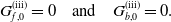(39) \begin{align} G_{f,0}^{\text{(iii)}}=0 \quad \text{and} \quad G_{b,0}^{\text{(iii)}}=0. \end{align}

4.3 Region (ii): local to the saturation front

Region (ii) is a slender region adjacent to region (iii), in which the fines rapidly undergo dissolution thereby boosting the concentration in the intergranular liquid to saturation. In order to appreciably change $c_l$ across this narrow region, and match together regions (i) and (iii), we require a large mass transfer rate from one of the sets of particles. It is only the smaller fines that are able to supply the requisite size flux through their surfaces. We use the method of dominant balance to determine the local variable transform in region (ii), for which the dissolution terms are in balance with diffusion in the fines and with advection and diffusion in the liquid terms. The solution in this region is found by making the following change of variables

(40) \begin{align} \epsilon w =z-s_d, \end{align}

under which equations (23)–(25) become:

(41) \begin{align} \frac {\phi _l}{\phi _T}\left ( \frac {\partial c_l}{\partial t} - \frac {\dot {s_d}}{\epsilon }\frac {\partial c_l}{\partial w} \right ) + \frac {1}{\epsilon }\frac {\partial {\mathcal F}_l}{\partial w} = { G_f + G_b}, \quad \quad {\mathcal F}_{l} = -\hat {D}_{\text{eff}} \frac {\partial c_{l}}{\partial w} + q c_l, \end{align}

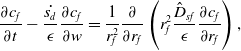(42) \begin{align} \frac {\partial c_{f}}{\partial t} - \frac {\dot {s_d}}{\epsilon }\frac {\partial c_f}{\partial w} = \frac {1}{r_f^{2}} \frac {\partial }{\partial r_f} \left ( r_f^{2} \frac {\hat {D}_{sf}}{\epsilon } \frac {\partial c_f}{\partial r_f} \right ),\end{align}

(43) \begin{align} \mbox{with} \quad - \frac {\hat {D}_{sf}}{\epsilon } \frac {\partial c_f}{\partial r_f} \Big {|}_{r_f=0} = 0 \quad \mbox{and} \quad -\frac {\hat {D}_{sf}}{\epsilon } \frac {\partial c_f}{\partial r_f} \Big {|}_{r_f=1} = Q_fG_f.\end{align}

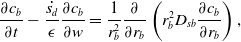(44) \begin{align} \frac {\partial c_{b}}{\partial t} - \frac {\dot {s_d}}{\epsilon }\frac {\partial c_b}{\partial w} = \frac {1}{r_b^{2}} \frac {\partial }{\partial r_b} \left ( r_b^{2} D_{sb} \frac {\partial c_b}{\partial r_b} \right ),\end{align}

(45) \begin{align} \mbox{with} \quad - D_{sb} \frac {\partial c_b}{\partial r_b} \Big {|}_{r_b=0} = 0 \quad \mbox{and} \quad -D_{sb} \frac {\partial c_b}{\partial r_b} \Big {|}_{r_b=1} = Q_bG_b.\end{align}

These equations need to match the solutions in region (iii) as $w \to \infty$ and the solution in region (i) as $w \to -\infty$ . The matching conditions can be written as

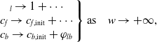(46) \begin{align} \left .\begin{array} c_l \to 1 + \cdots \\ c_{f} \to c_{f,\text{init}} + \cdots \\ c_b \to c_{b,\text{init}} + \varphi _{lb} \end{array}\right \} \mbox{as} \quad w \to +\infty, \end{align}

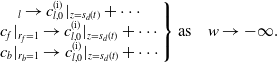(47) \begin{align} \left .\begin{array} c_l \to c_{l,0}^{\text{(i)}}|_{z=s_d(t)} + \cdots \\ c_{f}|_{r_f=1} \to c_{l,0}^{\text{(i)}} |_{z=s_d(t)} + \cdots \\ c_b|_{r_b=1} \to c_{l,0}^{\text{(i)}} |_{z=s_d(t)} + \cdots \end{array}\right \} \mbox{as} \quad w \to -\infty . \end{align}

We seek an asymptotic solution using the following expansions

(48) \begin{align} c_{l} = c_{l,0}^{\text{(ii)}}+ {o(1)}, \quad {c_{f}} = {c_{f,0}}^{\text{(ii)}}+ {o(1)}, \quad c_{b} = c_{b,0}^{\text{(ii)}} + {o(1)}, \end{align}

(49) \begin{align} {\mathcal F}_l = {\mathcal F}_{l,0}^{\text{(ii)}} + {o(1)}, \quad {\mathcal F}_f = {\mathcal F}_{f,0}^{\text{(ii)}} + {o(1)}, \quad {\mathcal F}_b = {\mathcal F}_{b,0}^{\text{(ii)}} + {o(1)}, \end{align}

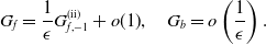(50) \begin{align} G_f = \frac {1}{\epsilon } G_{f,-1}^{\text{(ii)}}+ {o(1)}, \quad G_{b}= o \left ( \frac {1}{\epsilon } \right ).\end{align}

In what follows we seek only the lowest-order terms. Substituting the expansions (48)–(50) and balancing leading order terms in (41) yields

(51) \begin{align} - \dot {s_d} \frac {\phi _l}{\phi _T} \frac {\partial c_{l,0}^{\text{(ii)}}}{\partial w} + \frac {\partial {\mathcal F}_{l,0}^{\text{(ii)}}}{\partial w} = { G_{f,-1}^{\text{(ii)}} }\quad \mbox{where} \quad {\mathcal F}_{l,0}^{\text{(ii)}} = -\hat {D}_{\text{eff}} \frac {\partial c_{l,0}^{\text{(ii)}}}{\partial w} + q c_{l,0}^{\text{(ii)}}. \end{align}

Integrating the former of the two equations in (51) across region (ii) and imposing the matching conditions (46) and (47) leads to

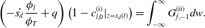(52) \begin{align} \left ( - \dot {s_d} \frac {\phi _l}{\phi _T} + q \right ) \left ( 1 - c_{l,0}^{\text{(i)}}|_{z=s_d(t)} \right ) = \int _{-\infty }^{\infty } {G_{f,-1}^{\text{(ii)}} }dw. \end{align}

Substituting the expansions (48)–(50) and balancing leading order terms in (42)–(43) leads to

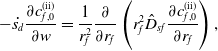(53) \begin{align} -\dot {s_d}\frac {\partial c_{f,0}^{\text{(ii)}}}{\partial w} = \frac {1}{r_f^{2}} \frac {\partial }{\partial r_f} \left ( r_f^{2} \hat {D}_{sf} \frac {\partial c_{f,0}^{\text{(ii)}}}{\partial r_f} \right ), \end{align}

(54) \begin{align} \mbox{with} \quad - \hat {D}_{sf} \frac {\partial c_{f,0}^{\text{(ii)}}}{\partial r_f} \Big {|}_{r_f=0} = 0 \quad \mbox{and} \quad -\hat {D}_{sf} \frac {\partial c_{f,0}^{\text{(ii)}}}{\partial r_f} \Big {|}_{r_f=1} = Q_fG_{f,-1}^{\text{(ii)}}. \end{align}

Multiplying through by $r_f^2$ and integrating over the radial domain and imposing the boundary conditions (54) gives

(55) \begin{align} -\dot {s}_d \int _0^1 r_f^2 \frac {\partial c_{f,0}^{\text{(ii)}}}{\partial w} dr_f = -Q_fG_{f,-1}^{\text{(ii)}}. \end{align}

This can then be integrated across the width of region (ii) yielding

(56) \begin{equation} -\dot {s}_d \int _{-\infty }^{+\infty } \int _0^1 r_f^2 \frac {\partial c_{f,0}^{\text{(ii)}}}{\partial w} dr_f dw = \int _{-\infty }^{+\infty }-Q_fG_{f,-1}^{\text{(ii)}} dw. \end{equation}

We can change the order of integration on the left hand side because $r_f$ and $w$ , i.e., the micro- and macroscopic coordinates respectively, are orthogonal (a foundational assumption of multiple scales homogenisation on which our model is based). Evaluating the integrals that result leads us to

(57) \begin{align} -\frac {\dot {s}_d}{3} \left ( c_{f,\text{init}} - c_{l,0}^{\text{(i)}}|_{z=s_d(t)} \right ) = -Q_f \int _{-\infty }^{+\infty } G_{f,-1}^{\text{(ii)}} dw. \end{align}

Eliminating the integral in (57), representing the fine dissolution rate, using (52) and the matching conditions (46)–(47), gives

(58) \begin{align} {\frac {\dot {s}_d}{3Q_f} \left ( c_{f,\text{init}} - c_{l,0}^{\text{(i)}}|_{z=s_d(t)} \right ) = \left ( - \dot {s_d} \frac {\phi _l}{\phi _T} + q \right ) \left ( 1 - c_{l,0}^{\text{(i)}}|_{z=s_d(t)} \right ).} \end{align}

The result (58) is one of the key equations that will form the reduced model, see Section 4.5. Equation (58) is a concise statement of the conservation of solubles across region (ii) and serves as an ODE that (when coupled with the remainder of the reduced model) will allow us to determine the position $z=s_d(t)$ , separating regions (i) and (iii). For consistency with the initially dry coffee bed, we will require that $s_d|_{t=0}=0$ , see (74), and (58) pertains until such a time that $s_d(t)=1$ , i.e., when region (ii) reaches the bottom of the basket, after which (58) is no longer necessary because region (i) occupies the entirety of the basket and hence there is no longer a demarcation between regions (i) and (iii). Finally, we note that the leading terms in equation (44) that governs the concentration in the boulders throughout region (ii) asserts that

(59) \begin{align} \frac {\partial c_{b,0}^{\text{(ii)}}}{\partial w} = 0 \end{align}

whose solution, along with the matching condition (46) is

(60) \begin{align} c^{\text{(ii)}}_{b,0} = c_{b,\text{init}}+\varphi _{lb}. \end{align}

The remaining equations for the leading order concentrations in the fines and liquid could be solved if necessary but, as we shall show, the analysis presented here gives sufficient information to evolve the position of the saturation front.

4.4 Region (i): slowly reacting region

For $t=O(1)$ , once the fines near the inlet have been dissolved to such an extent that they are close to being in equilibrium with the surrounding water ( $c_f|_{r_f=1} \approx c_l$ ), region (i) is formed in which the dissolution continues controlled by the rate at which solubles can be transported from the interior of the boulders to their surface. We seek an asymptotic solution in region (i) of the following form

(61) \begin{align} c_{l} = c_{l,0}^{\text{(i)}}+ {o(1)}, \quad {c_{f}} = {c^{\text{(i)}}_{f,0}}+ {o(1)}, \quad c_{b} = c_{b,0}^{\text{(i)}} + {o(1)},\end{align}

(62) \begin{align} {\mathcal F}_l = {\mathcal F}_{l,0}^{\text{(i)}} + {o(1)}, \quad {\mathcal F}_f = {\mathcal F}_{f,0}^{\text{(i)}} + {o(1)}, \quad {\mathcal F}_b = {\mathcal F}_{b,0}^{\text{(i)}} + {o(1)}, \end{align}

(63) \begin{align} G_f = G_{f,0}^{\text{(i)}} + {o(1)}, \quad G_{b}= G_{b,0}^{\text{(i)}} + {o(1)}.\end{align}

As in the previous regions, in what follows we seek only the lowest-order terms. Substituting the expansions (61)–(63) and balancing leading order terms in (25) reveals that diffusion through the fines is sufficiently fast that at leading order their internal concentration is independent of $r_f$ . Hence, on multiplying (25) through by $r_f^2$ , integrating across $r_f \in (0,1)$ , and imposing the boundary conditions (26) at leading order, we discern that

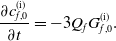(64) \begin{align} \frac {\partial c_{f,0}^{\text{(i)}}}{\partial t} = - 3 Q_f G_{f,0}^{\text{(i)}}. \end{align}

Inserting the expansion (61)–(63) into the dissolution rates, balancing at leading order, and recalling that the concentration in the fines is uniform in $r_f$ reveals that

(65) \begin{align} c_{b,0}^{\text{(i)}}(z,r_b,t)|_{r_b=1}=c_{f,0}^{\text{(i)}}(z,t)=c_{l,0}^{\text{(i)}}(z,t) \end{align}

Balancing leading order terms in (23) leads to

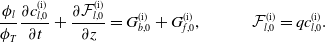(66) \begin{align} \frac {\phi _l}{\phi _T} \frac {\partial c_{l,0}^{\text{(i)}}}{\partial t} + \frac {\partial {\mathcal F}_{l,0}^{\text{(i)}}}{\partial z} = {{G}_{b,0}^{\text{(i)}} + G_{f,0}^{\text{(i)}}}, \qquad \quad {\mathcal F}^{\text{(i)}}_{l,0} = q c^{\text{(i)}}_{l,0}. \end{align}

Eliminating ${\mathcal F}_{l,0}$ and $G_{f,0}$ from (66a) using (66b) and (64) leads us to an equation for conservation of solubles in the region $0\le z \le s_d(t)$

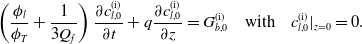(67) \begin{align} \left ( \frac {\phi _l}{\phi _T} + {\frac {1}{3Q_f}} \right ) \frac {\partial c^{\text{(i)}}_{l,0}}{\partial t} + q \frac {\partial c^{\text{(i)}}_{l,0}}{\partial z} = {G_{b,0}^{\text{(i)}}} \quad \mbox{with} \quad c^{\text{(i)}}_{l,0}|_{z=0}=0. \end{align}

Dissolution from a boulder begins when the saturation front passes (i.e., when the boulder enters region (i)) and it is exposed to non-saturated water for the first time. We denote $t_0 = s_d^{-1}(z)$ to be the time at which the saturation interface passes a given location $z$ . Thus $t_0(z)$ is the first time at which the boulder at position $z$ becomes wet. The pores within the boulders entering region (i) have been filled with saturated liquid, see (37), and hence their internal concentration on entering region (i) is given by (60), in agreement with the matching condition (47). Thus, the leading order transport problem within the boulders defined for $0\le r_b \le 1$ , $t \ge t_0(z)$ is

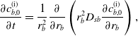(68) \begin{align} \frac {\partial c_{b,0}^{\text{(i)}}}{\partial t} = \frac {1}{r_b^{2}} \frac {\partial }{\partial r_b} \left ( r_b^{2} D_{sb} \frac {\partial c_{b,0}^{\text{(i)}}}{\partial r_b} \right ),\end{align}

(69) \begin{align} -D_{sb} \frac {\partial c_{b,0}^{\text{(i)}}}{\partial r_b} \Big {|}_{r_b=0} = 0, \quad c_{b,0}^{\text{(i)}}|_{r_b=1}=c_{l,0}^{\text{(i)}} \quad \mbox{and} \quad c_{b,0}^{\text{(i)}}|_{{t=t_0(z)}} = c_{b,\text{init}} + \varphi _{lb}.\end{align}

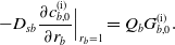(70) \begin{align} -D_{sb} \frac {\partial c_{b,0}^{\text{(i)}}}{\partial r_b} \Big {|}_{r_b=1} = Q_bG_{b,0}^{\text{(i)}} .\end{align}

Equations (68)–(70) can be viewed as defining a relationship between the leading order concentration in the liquid $c_{l,0}$ and the leading order flux of solubles at the boulder’s surface $G_{b,0}$ . In fact, because the transport problem is linear this relationship can be determined analytically (details are given in the supplementary material); it reads as follows:

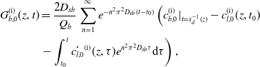(71) \begin{align} G_{b,0}^{\text{(i)}}(z,t) &= \frac {2 D_{sb}}{Q_b} \sum _{n=1}^{\infty } e^{-n^2 \pi ^2 D_{sb}(t-t_0)}\left (c_{b,0}^{\text{(i)}}|_{t=s_d^{-1}(z)} -c_{l,0}^{\text{(i)}}(z,t_0) \right .\nonumber \\ &\left .-\int _{t_0}^{t}\dot {c_{l,0}}^{\text{(i)}}(z,\tau )e^{n^2 \pi ^2 D_{sb}\tau } \text{d}\tau \right ), \end{align}

The combination of (67) and (71) is a closed problem to be solved for the leading order concentration in the liquid, which can be written elegantly under the change of variables

(72) \begin{align} \chi = z, \qquad \tau = -\frac {1}{q} \left ( \frac {\phi _l}{\phi _T} + {\frac {1}{3Q_f}} \right ) z + t, \qquad \tilde {c}(\chi, \tau ) = c_{l,0}^{\text{(i)}}(z,t), \end{align}

as

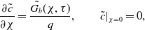(73) \begin{align} \frac {\partial \tilde {c}}{\partial \chi } = {\frac {\tilde {G_b}(\chi, \tau )}{q} }, \qquad \tilde {c}|_{\chi = 0} = 0, \end{align}

where $\tilde {G_b}(\chi, \tau ) = G_{b,0}^{\text{(i)}}(z,t)$ , i.e., that arrived at by applying the variable transform (72) to (71). This change of independent variables amounts to the application of the method of characteristics; the PDE (66) is reduced to an ODE, namely (73), that is satisfied along the characteristic lines. Replacing an advection-reaction PDE (66), with a relatively simple ODE leads to a significant reduction in mathematical complexity and in turn to reduced computational cost when the resulting problem is solved numerically. Furnishing solutions to this problem (72)-(73) requires a numerical method. Once $\tilde {c}$ has been found, the leading order concentrations in the grains and liquid can be found readily by backsubstitution.

4.5 The asymptotically reduced model

In the wake of the asymptotic analysis we now summarise the equations that must be solved in order to predict the quantity of primary interest, namely, the concentration of the liquid exiting the espresso bed. Rearranging (58) yields the following ODE to be solved for the position of the saturation front, in terms of the concentration in the liquid at the edge of region (i):

(74) \begin{align} \frac {ds_d}{dt} = q \left ( \frac {\phi _l}{\phi _T} + {\frac {1}{3Q_f}} \frac {c_{f,\text{init}}-c^{\text{(i)}}_{l,0}|_{z=s_d(t)}}{1-c^{\text{(i)}}_{l,0}|_{z=s_d(t)}} \right )^{-1} \quad \mbox{with} \quad s_d|_{t=0}=0. \end{align}

This must be solved in tandem with (73), an ODE for the concentration in the liquid, until such a time that $s_d(t)=1$ . Beyond this instance, the concentration at the exit is determined wholly by (73). Thus, the concentration at the exit (to leading order) for all time is given by

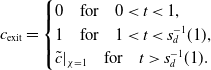(75) \begin{align} c_{\text{exit}} = \begin{cases} 0 \quad \text{for} \quad 0\lt t\lt 1,\\ 1 \quad \text{for} \quad 1\lt t\lt s_d^{-1}(1),\\ \tilde {c}|_{\chi =1} \quad \text{for} \quad t\gt s_d^{-1}(1). \end{cases} \end{align}

We present a numerical method for solving this problem doing so in the subsequent section.

We return to the question raised in Section 2.7 of whether a saturated layer forms immediately above the wetting front, i.e., whether regions (ii) and (iii) form. In retrospect, we now observe that if on solving the asymptotically reduced model $s_d\gt s_w$ , at any time, then at that time the asymptotic structure of the model that we have presented breaks down and regions (ii) and (iii) along with the saturated layer cease to exist. In such a scenario, the solution throughout the wet part of the bed is unsaturated and must be found by solving the problem described in the supplementary information.

5 Results

We now validate the asymptotic analysis by comparing numerical solutions of the full model to those of the asymptotically reduced one. Throughout we use the following set of parameters:

(76) \begin{align} \phi _f = 0.64, \quad \phi _{b} &= 0.16, \quad \phi _l = 0.2, \quad \varphi _{lb} = 0, \end{align}

(77) \begin{align} \epsilon \ll 1, \quad D_{sf} &= 1/\epsilon, \quad D_{sb} = 1, \quad D_{\text{eff}} = O( \epsilon ) \end{align}

and we will select a range of small values of $\epsilon$ to demonstrate convergence. The value of $\varphi _{lb} = 0$ is chosen to compare the results of the full model and the reduced model. The reason for this is non-zero values of this parameter cause additional complications in the numerical implementation for the full model and so $\varphi _{lb} = 0$ allows for a direct comparison. The details of the numerical schemes used to solve the full and the reduced model are given in the supplementary material.

5.1 Validation of the reduced model

Figures 3 and 4 show the comparisons between the full model (23)–(29) and the reduced model (73)–(75) for varying values of $\epsilon$ . Care was taken to ensure that all numerical errors are sufficiently small that any discrepancies between the full and numerical solutions can be attributed to the errors associated with truncating the asymptotic expansions. Figure 5 shows how the discrepancy between the full and reduced models decreases as $\epsilon$ is reduced as expected. Ideally, this comparison would have been extended to yet smaller values of $\epsilon$ . However, reducing $\epsilon$ beyond $3\times 10^{-3}$ renders the computations prohibitively expensive. As $\epsilon$ is reduced, gradients in the vicinity of region (ii) become larger and therefore a finer spatial mesh is required in order to maintain accuracy. Moreover, because region (ii) transits through the whole of the bed, a highly refined spatial mesh is required everywhere. An adaptive spatial mesh may be able to alleviate this difficulty to an extent, but implementing such an advanced numerical approach is beyond the scope of this study.

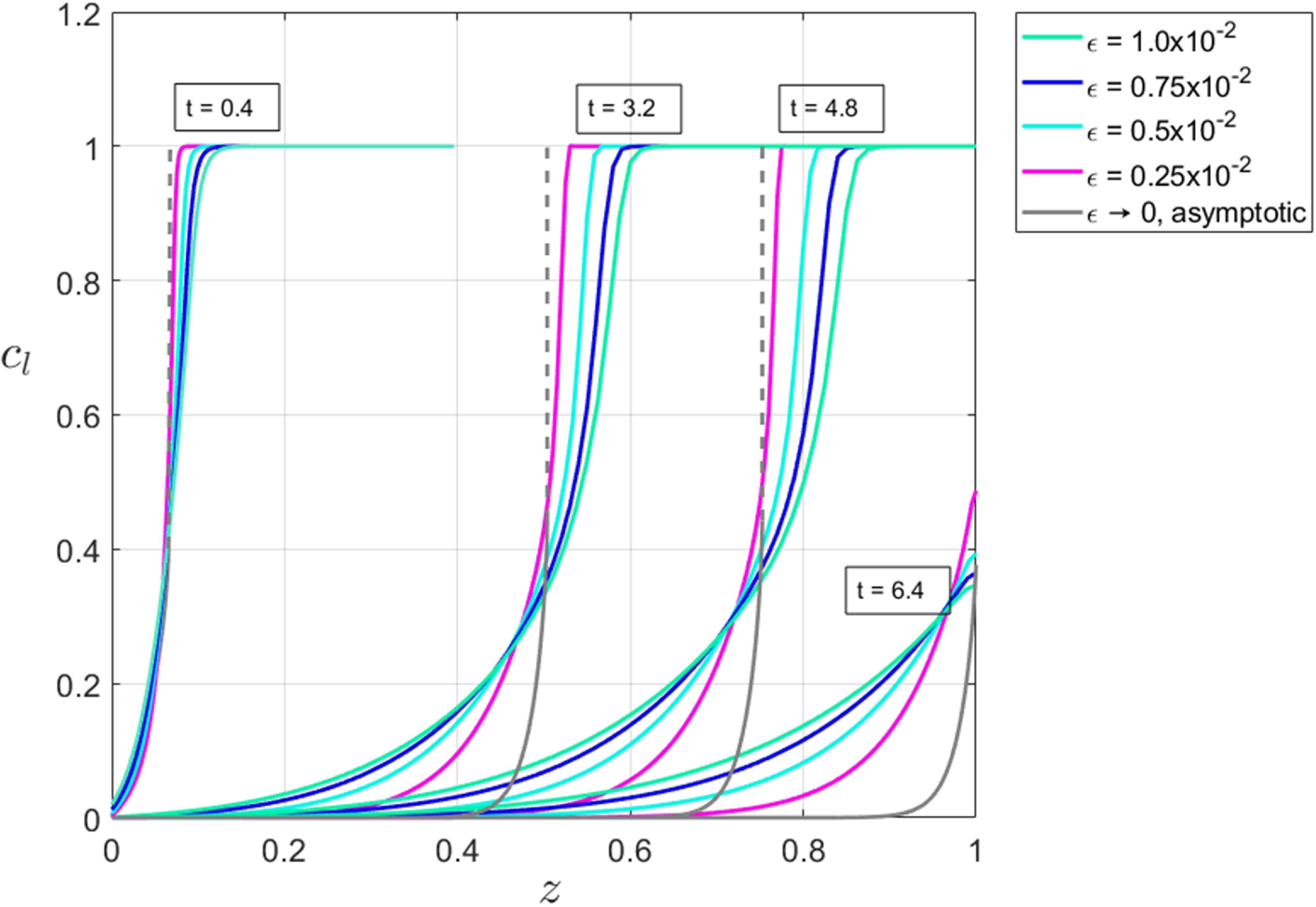
Figure 3. Concentration profiles in the liquid phase as the saturation front advances. Groups of curves given at $t = 0.4, 3.2, 4.8, 6.4$ . Solutions for non-zero values of $\epsilon$ are obtained by solving the full model numerically and the asymptotic solution is obtained by the numerical solver for the reduced model. The vertical dashed lines mark the position of region (ii), $z=s_d(t)$ , according to the solution of the asymptotically reduced model.

These difficulties in solving the full model underline the value of the reduced model. To make this concrete, using a typical modern desktop computer with 4 cores and 32 GB of RAM (and insisting that both schemes result in solutions accurate to three digits) the reduced problem has a typical compute time of around 10 s whereas the full model takes around 1000s. This pertains for $\epsilon =10^{-2}$ , which is not yet small enough to be physically relevant. This significant speed-up is not only valuable in its own right but also opens the door to optimisation studies (e.g., tuning parameters to achieve a target brew strength) which require many model solutions and would therefore be highly impractical with the long run times required by the full model. Of course, these benefits of the reduced model must be understood with the caveat that they only pertain in regimes where $\epsilon \ll 1$ .

5.2 Interpretation of typical solutions

In Figure 3 we see the saturation front progressing down the bed, marked on each group of curves at the end of the solid yellow lines. The asymptotically reduced model gives us the solution in regions (i) and (iii) and they are connected by a region (ii) of width $\epsilon \to 0$ in which the concentration in the liquid is rapidly increasing. The shape of the solution in region (ii) is not fundamental due to the width of the region, therefore we chose to match the regions with a linear concentration profile in region (ii) displayed by the dashed yellow lines. When the saturation front reaches the outlet $s_d = 1$ , at approximately $t = 6.4$ (dimensionless), we no longer observe regions (ii) and (iii) and the entire bed is described by the solution in region (i).

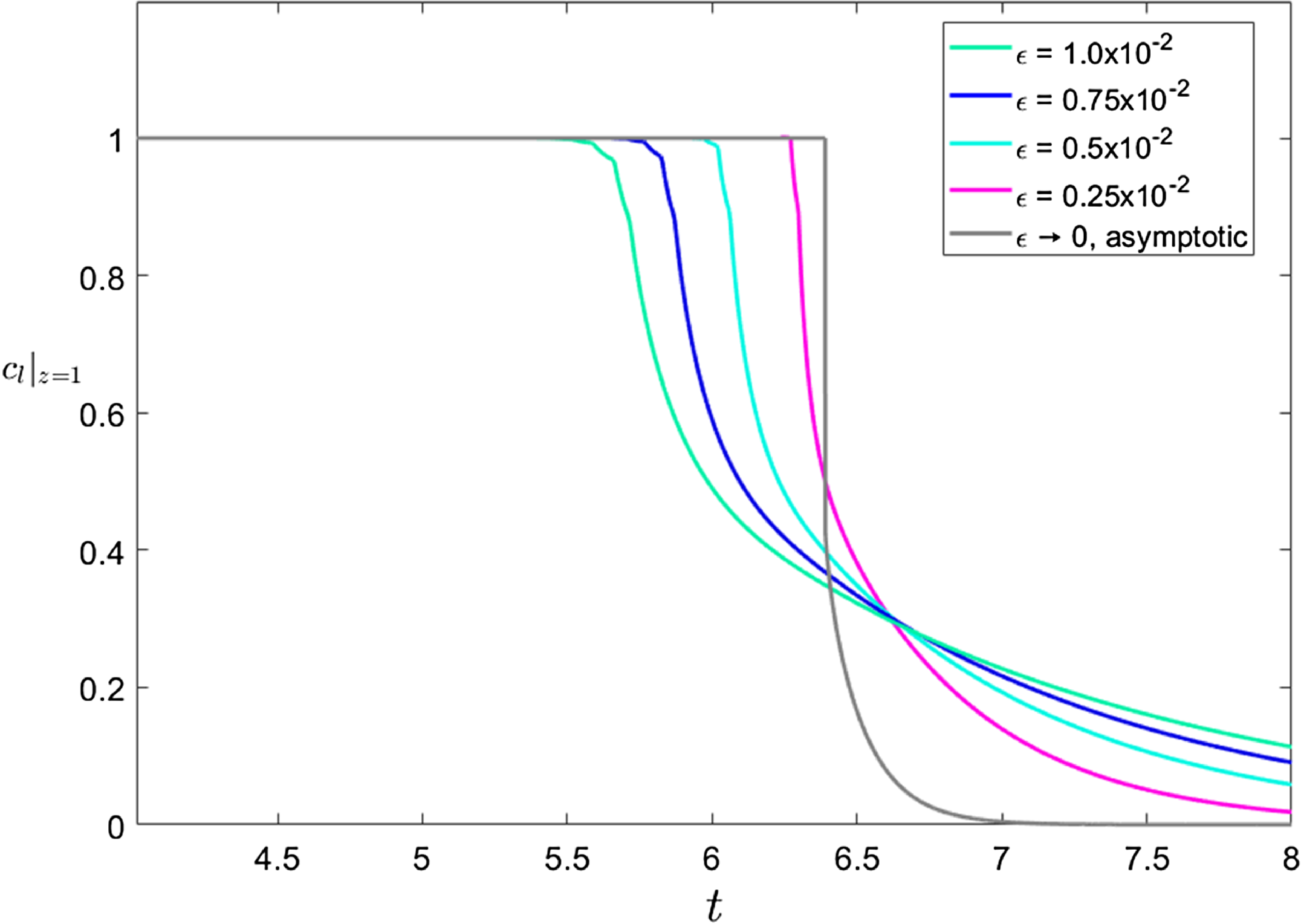
Figure 4. Time-resolved concentration at the outlet. Solutions for non-zero values of $\epsilon$ are obtained by solving the full model numerically and the asymptotic solution is obtained by the numerical solver for the reduced model.

Figure 5. An error analysis of the results in Figure 3. The error measure is defined as $\mathcal{E}(t) = \sum _{i=1}^{i=n} (c_l^{\text{num}}|_{x=x_i} - c_l^{\text{asy}}|_{x=x_i})^2 / n$ in which $x_i$ are the locations of the mesh points; and the superscripts are used to distinguish the numerical solution of the full model (‘num’) from the numerical solution of the asymptotically reduced model (‘asy’).

Dissolution in boulders begins once the saturation front passes through and they are in region (i). We note that due to our choice of constant flow and the current set of parameters, concentration profiles in the interior of the grains after dissolution begin to appear to be identical, see Figures 6 and 7; however, this is not common for all parameter sets. The concentration in the fines in region(i) is constant in their interior due to their small size and fast dissolution rate and it is in balance with the concentration in the surrounding liquid and on the surfaces of the boulders according to the solution (65). Due to this balance, the concentration on the surface of a boulder located at $z=1$ as a function of time is also given in Figure 4 by the asymptotic solution.

Due to saturation of the bed, for a short time after wetting is complete, the liquid that comes out of the bed is fully saturated with solubles, see Figure 4. After saturation passes, the concentration is monotonically decreasing until the end of the brew. When pulling an espresso shot this effect is referred to as blonding. It describes the change of the colour of the liquid from dark brown to very light pale blond is used as an indication to end the shot. In future work, we intend to compare the reduced model to experimental data on time-resolved concentration at the outlet.

Figure 6. Concentration profiles inside the grains located at $z = 0.1$ . Solid lines show profiles in the interior of the boulders at the listed times. Dashed lines show constant concentration across the interior of the fines at corresponding times.

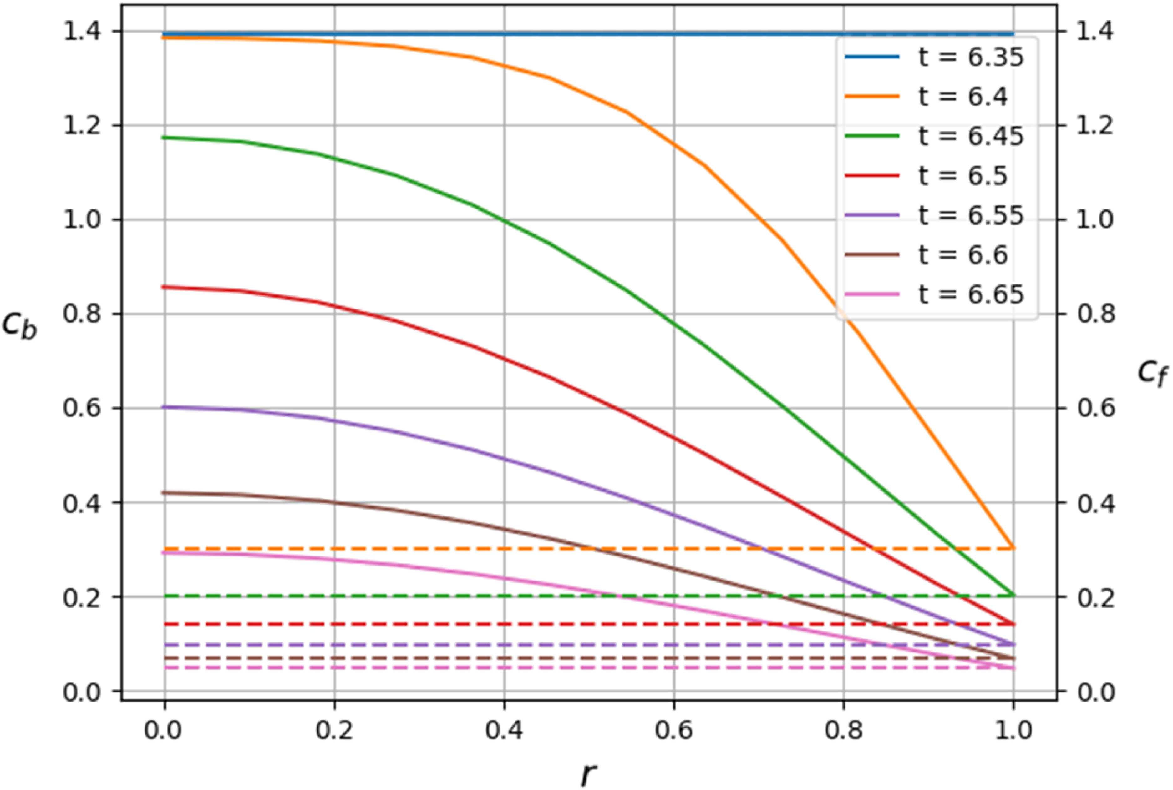
Figure 7. Concentration profiles inside the grains located at $z = 1$ . Solid lines show profiles in the interior of the boulders at the listed times. Dashed lines show constant concentration across the interior of the fines at corresponding times.

6 Conclusion

This work presents a novel model for espresso brewing that captures the initial infiltration phase of the water including filling up the pore space between grains and inside the boulders. As we have shown, a significant portion of the solubles that end up in the cup are extracted during this infiltration phase; as such it is important to model this accurately. We have also provided a systematic derivation of a reduced model which captures all the important features of the full model, yet is significantly cheaper to solve and easier to interpret.

The utility of this work is in understanding how the physical processes and material properties/parameters affect the extraction and ultimately the TDS, BS, and EY of espresso. Ultimately, we hope that this deeper insight will help make quantitative statements and predictions about the flavours of coffee.

The non-dimensionalisation of the model reveals that for typical espresso brewing conditions there are several small parameters corresponding to (a) fast dissolution reaction rates, (b) fast transport through the interior of the fines and (c) relatively small diffusive fluxes in the water. The asymptotic analysis based on the magnitude of these parameters shows that the structure of the solution to an asymptotically reduced model comprises of three regions where we can identify dominant physical processes in each one, provided that the fines are able to supply enough solubles to saturate the liquid. Region (iii) resides adjacent to the wetting front and here, the water is completely saturated with coffee solubles and there is no dissolution from the grains. Region (i) is adjacent to the inlet, the incoming water gradually dissolves the boulders and the concentrations of solubles in the liquid and on the surfaces of the grains are in equilibrium. The solution is completed by a narrow region (ii), which separates regions (i) and (iii). A particularly interesting aspect is that the position of region (ii) is unknown a priori and its progressive movement downwards in the bed must be determined as part of the solution to the problem. Here, the fines rapidly dissolve thereby boosting the concentration of solubles in the liquid to saturation. As is described in detail in the supplementary material, in the case that saturation does not occur, the analysis in regions (i) and (ii) is broadly similar whilst region (iii) ceases to exist.

In parameter regimes where the asymptotic analysis pertains, a numerical solution to the reduced model can be used in place of the full model; allowing solutions to be obtained orders of magnitude more quickly and without compromising accuracy. This opens the door for various practical applications such as incorporation of concentration prediction in espresso machine software that could compute results significantly faster than the actual brewing process.

Future work that supplements this paper will disclose additional details and optimisation methods applied to the numerical schemes and will compare model solutions to time-resolved coffee concentration in the liquid gathered from experimental data. This analysis can be further expanded by tracking groups of chemicals that can be easily measured during experiments such as acidic content that could be directly correlated to the taste of a beverage. Being able to mathematically distinguish not only strength and concentration but also subjective characteristics such as taste or aroma remains the ultimate inspiration and motivation for advancing this work.