Echeloned Spaces

Abstract

We introduce the notion of echeloned spaces – an order-theoretic abstraction of metric spaces. The first step is to characterize metrizable echeloned spaces. It turns out that morphisms between metrizable echeloned spaces are uniformly continuous or have a uniformly discrete image. In particular, every automorphism of a metrizable echeloned space is uniformly continuous, and for every metric space with midpoints, the automorphisms of the induced echeloned space are precisely the dilations.

Next, we focus on finite echeloned spaces. They form a Fraïssé class, and we describe its Fraïssé-limit both as the echeloned space induced by a certain homogeneous metric space and as the result of a random construction. Building on this, we show that the class of finite ordered echeloned spaces is Ramsey. The proof of this result combines a combinatorial argument by Nešetřil and Hubička with a topological-dynamical point of view due to Kechris, Pestov and Todorčević. Finally, using the method of Katětov functors due to Kubiś and Mašulović, we prove that the full symmetric group on a countable set topologically embeds into the automorphism group of the countable universal homogeneous echeloned space.

The notion of a metric is ubiquitous in mathematics. This is no doubt due to its great versatility for capturing information of topological, geometrical and order-theoretical nature.

The first abstract definitions of metric spaces given by Fréchet (see [8, p.772], [9, p.18]) and Hausdorff (see [11, p.211]) had as a goal to capture the notion of convergence. This lead to the notion of a topology or of a uniformity induced by a metric and is certainly the main focus of research concerning metric spaces.

Geometrical aspects of abstract metric spaces were first treated by Menger (see [19]). He studied convexity of metric spaces, and he examined the basic properties of betweenness relations. A complete axiomatization of betweenness relations in metric spaces was given only recently by Chvátal (see [6]).

As an example of an order-theoretic aspect of metric spaces, we mention the phenomenon of boundedness. The notion of abstract boundedness (now better known as bornology) was introduced and studied by Hu (see [13]). In particular, Hu characterized metrizable bornologies.

Last but not least, every metric space gives rise to a (bounded) coarse structure in the sense of Roe (see [24]). Roughly speaking, such a coarse structure captures geometric properties of the space on a large scale (i.e., up to a uniformly bounded error).

All the structures mentioned above have one thing in common: they are definable from metric spaces while the actual numerical distance between two points is of no great importance. For instance, a metric may be scaled by a positive real number without making any difference concerning convergence, boundedness or convexity. For topological considerations, only the very small distances are of interest; for coarse geometries, large distances are relevant; and for geometrical considerations, mainly qualitative properties like collinearity stand in the focus. Finally, in bornological considerations the order relation between distances is crucial.

Motivated by these observations, in this paper, we introduce echeloned spaces. These are spaces in which the closeness between pairs of points cannot be measured but only compared. Echeloned spaces appear to capture very well the order-theoretic aspects of metric spaces.

It should be mentioned that a notion similar to echeloned spaces was suggested by Pestov when discussing nearest neighbor classifiers in machine learning [23, Observação 5.4.40]. In contrast to our approach, Pestov compares distances of points to a given point.

When finishing this paper, we became aware of the work [16], in which Keller and Petrov, motivated by the use of ordinal data analysis in machine learning, introduced a notion equivalent to echeloned spaces, under the name ordinal spaces. Their results cover, among others, balls in echeloned spaces and embeddings into Euclidean spaces and are rather different than ours. As the term ‘ordinal space’ is already in use in general topology (denoting a well-ordered set with the interval topology; see, for example, [7, Chapter 3, §3]), we use the term ‘echeloned space’ to avoid confusions.

In Section 1, after the basic definitions, we settle the question of metrizability of echeloned spaces (see Proposition 1.11).

Section 2 is concerned with morphisms between metrizable echeloned spaces. The main result of this section is a characterization of the automorphisms of echeloned spaces induced by metric spaces with midpoints (see Proposition 2.8).

Section 3 contains the proof of the existence of a countable universal homogeneous echeloned space $\mathbf {F}$ (using Fraïssé’s Theorem). It is shown that this space is not the echeloned space induced by the countable universal homogeneous rational metric space, a.k.a. the rational Urysohn space (see Corollary 3.6). We proceed to showing that the edge-coloured graph induced by $\mathbf {F}$ is in fact universal and homogeneous as an edge-coloured graph (see Theorem 3.17), and we give a probabilistic construction of this graph (see Proposition 3.19).

In Section 4, we show that the class of finite ordered echeloned spaces has the Ramsey property in the sense of [20] (see Theorem 4.6). The proof combines a combinatorial result by Hubička and Nešetřil [14] with the Kechris-Pestov-Todorčević correspondence [15].

In Section 5, it is shown that the category of finite echeloned spaces with embeddings may be endowed with a Katětov functor in the sense of [17]. As a direct consequence, we obtain that the automorphism group of the countable universal homogeneous echeloned space contains the full symmetric group on a countable set as a closed topological subgroup.

Throughout the paper, we use standard model-theoretic notation and notions; see [12]. For additional notions and notation concerning homogeneous structures, we refer to [18].

1 Echeloned spaces

We define echeloned spaces as structures whose pairs of points are comparable.

Definition 1.1. Let X be a nonempty set. Then, a pair $\mathbf {X}=(X,\leqslant _{\mathbf {X}})$ is called an echeloned space if $(X^2,\leqslant _{\mathbf {X}})$ is a prechain¹ satisfying

1. (i) for all $x, y, z \in X$ : $(x,x) \leqslant _{\mathbf {X}} (y, z)$ ,

2. (ii) for all $x, y, z \in X$ , if $(y, z) \leqslant _{\mathbf {X}} (x,x)$ , then $y = z$ , and

3. (iii) for all $x, y \in X$ : $(x, y) \leqslant _{\mathbf {X}} (y,x)$ .

The relation $\leqslant _{\mathbf {X}}$ is called an echelon on X.

Given an echelon $\leqslant _{\mathbf {X}}$ on a set X, we introduce $\sim _{\mathbf {X}}\, \subseteq X^2$ as follows:

$$\begin{align*}(x_1, y_1) \sim_{\mathbf{X}} (x_2, y_2) \quad :\Longleftrightarrow \quad (x_1, y_1) \leqslant_{\mathbf{X}} (x_2, y_2) \quad \textrm{ and } \quad (x_2, y_2) \leqslant_{\mathbf{X}} (x_1, y_1).\end{align*}$$

Remark 1.2. Formally, one could have introduced echeloned spaces as relational structures over a signature $\{\lesssim \}$ , where $\operatorname {ar}(\lesssim ) = 4$ . Then, an echeloned space $(X, \leqslant _{\mathbf {X}})$ would in fact be a $\{\lesssim \}$ -structure $\mathbf {X} = (X, \lesssim _{\mathbf {X}})$ where $(x_1, y_1, x_2, y_2) \in {} \lesssim _{\mathbf {X}}$ if and only if $(x_1, y_1) \leqslant _{\mathbf {X}} (x_2, y_2)$ . This translation suggests a natural definition for homomorphisms and embeddings between echeloned spaces: if $\mathbf {X}$ and $\mathbf {Y}$ are two echeloned spaces, then a map $f\colon X\to Y$ is going to be called a homomorphism (embedding) from $\mathbf {X}$ to $\mathbf {Y}$ if and only if it is a homomorphism (embedding) between their corresponding $\{\lesssim \}$ -structures $(X,\lesssim _{\mathbf {X}})$ and $(Y,\lesssim _{\mathbf {Y}})$ .

Clearly, for any echeloned space $\mathbf {X} = (X, \leqslant _{\mathbf {X}})$ , the relation $\sim _{\mathbf {X}}$ is an equivalence relation on $X^2$ . The echelon $\leqslant _{\mathbf {X}}$ naturally induces a linear ordering on the quotient set ${X^2}/{\sim _{\mathbf {X}}}$ , written in symbols as $\leqslant _{E(\mathbf {X})}$ , as follows:

$$\begin{align*}\quad [(x_1, x_2)]_{\sim_{\mathbf{X}}} \leqslant_{E(\mathbf{X})} [(y_1, y_2)]_{\sim_{\mathbf{X}}} \quad :\Longleftrightarrow \quad (x_1, x_2) \leqslant_{\mathbf{X}} (y_1, y_2). \end{align*}$$

We shall refer to as the echeloning of $\mathbf {X}$ . Lastly, let $\eta _{\mathbf {X}} \colon X^2 \twoheadrightarrow E(\mathbf {X})$ be the quotient map.

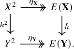
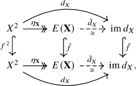
Lemma 1.3. Let $\mathbf {X}$ and $\mathbf {Y}$ be two echeloned spaces. Then, a map $h \colon X \to Y$ is a homomorphism from $\mathbf {X}$ to $\mathbf {Y}$ if and only if there exists a (necessarily unique) homomorphism of ordered sets $\hat {h} \colon E(\mathbf {X}) \to E(\mathbf {Y})$ for which $\hat {h} \circ \eta _{\mathbf {X}} = \eta _{\mathbf {Y}} \circ h^2$ ; that is, the diagram below commutes:

Proof. ‘ $\Rightarrow $ ’: First, assume that $h \colon X \to Y$ is a homomorphism between the echeloned spaces $\mathbf {X}$ and $\mathbf {Y}$ . Define $\hat {h} \colon {X^2}/{\sim _{\mathbf {X}}} \to {Y^2}/{\sim _{\mathbf {Y}}},\, [(x_1, x_2)]_{\sim _{\mathbf {X}}} \mapsto [(h(x_1), h(x_2))]_{\sim _{\mathbf {Y}}}$ . First, we show that it is well defined. Let $x_1, x_2, x_1^{\prime }, x_2^{\prime } \in X$ and $(x_1, x_2) \sim _{\mathbf {X}} (x_1^{\prime }, x_2^{\prime })$ ; that is, $[(x_1, x_2)]_{\sim _{\mathbf {X}}} = [(x_1^{\prime }, x_2^{\prime })]_{\sim _{\mathbf {X}}}$ . Then, $(h(x_1), h(x_2)) \sim _{\mathbf {Y}} (h(x_1^{\prime }), h(x_2^{\prime }))$ since h preserves $\leqslant _{\mathbf {X}}$ . Consequently,

$$\begin{align*}\hat{h}([(x_1, x_2)]_{\sim_{\mathbf{X}}}) = [(h(x_1), h(x_2))]_{\sim_{\mathbf{Y}}} = [(h(x_1^{\prime}), h(x_2^{\prime}))]_{\sim_{\mathbf{Y}}} = \hat{h}([(x_1^{\prime}, x_2^{\prime})]_{\sim_{\mathbf{X}}}). \end{align*}$$

Next, we prove that $\hat {h}$ preserves $\leqslant _{E(\mathbf {X})}$ . Take any $x_1, x_2, x_1^{\prime }, x_2^{\prime } \in X$ such that $[(x_1, x_2)]_{\sim _{\mathbf {X}}} \leqslant _{E(\mathbf {X})} [(x_1^{\prime }, x_2^{\prime })]_{\sim _{\mathbf {X}}}$ . By definition, this means that $(x_1, x_2) \leqslant _{\mathbf {X}} (x_1^{\prime }, x_2^{\prime })$ . Consequently, given that h is a homomorphism, it holds that $(h(x_1), h(x_2)) \leqslant _{\mathbf {Y}} (h(x_1^{\prime }), h(x_2^{\prime }))$ . So,

$$\begin{align*}\hat{h}([(x_1, x_2)]_{\sim_{\mathbf{X}}}) = [(h(x_1), h(x_2))]_{\sim_{\mathbf{Y}}} \leqslant_{E(\mathbf{Y})} [(h(x_1^{\prime}), h(x_2^{\prime}))]_{\sim_{\mathbf{Y}}} = \hat{h}([(x_1^{\prime}, x_2^{\prime})]_{\sim_{\mathbf{X}}}).\end{align*}$$

Finally, we show that for our choice of $\hat {h}$ , the above diagram commutes. Take any $x_1, x_2 \in X$ . Then,

$$\begin{align*}\hat{h} \circ \eta_{\mathbf{X}} (x_1, x_2) = \hat{h} ([(x_1, x_2)]_{\sim_{\mathbf{X}}}) = [(h(x_1), h(x_2))]_{\sim_{\mathbf{Y}}} = \eta_{\mathbf{Y}}(h(x_1), h(x_2)) = \eta_{\mathbf{Y}} \circ h^2 (x_1, x_2), \end{align*}$$

which is what we needed to show.

‘ $\Leftarrow $ ’: Assume $\hat {h} \colon E(\mathbf {X}) \to E(\mathbf {Y})$ is a homomorphism and $h \colon X \to Y$ a map such that $\hat {h} \circ \eta _{\mathbf {X}} = \eta _{\mathbf {Y}} \circ h^2$ . We prove h is a homomorphism from $\mathbf {X}$ to $\mathbf {Y}$ . Take any $x_1, x_2,x_1^{\prime }, x_2^{\prime } \in X$ such that $(x_1, x_2) \leqslant _{\mathbf {X}} (x_1^{\prime }, x_2^{\prime })$ . This is equivalent to saying that

$$\begin{align*}\eta_{\mathbf{X}}(x_1, x_2) = [(x_1, x_2)]_{\sim_{\mathbf{X}}} \leqslant_{E(\mathbf{X})} [(x_1^{\prime}, x_2^{\prime})]_{\sim_{\mathbf{X}}} = \eta_{\mathbf{X}}(x_1^{\prime}, x_2^{\prime}), \end{align*}$$

by definition of $\leqslant _{E(\mathbf {X})}$ . It follows that

$$\begin{align*}\hat{h}\circ \eta_{\mathbf{X}} (x_1, x_2) = \hat{h} ([(x_1, x_2)]_{\sim_{\mathbf{X}}}) \leqslant_{E(\mathbf{Y})} \hat{h}([(x_1^{\prime}, x_2^{\prime})]_{\sim_{\mathbf{X}}}) = \hat{h}\circ \eta_{\mathbf{X}} (x_1^{\prime}, x_2^{\prime}).\end{align*}$$

Now, from the commutativity of the given diagram, that is equivalent to

$$\begin{align*}\eta_{\mathbf{Y}}(h(x_1), h(x_2)) = \eta_{\mathbf{Y}} \circ h^2 (x_1, x_2) \leqslant_{E(\mathbf{Y})} \eta_{\mathbf{Y}} \circ h^2 (x_1^{\prime}, x_2^{\prime}) = \eta_{\mathbf{Y}}(h(x_1^{\prime}), h(x_2^{\prime})).\end{align*}$$

In other words, $[(h(x_1), h(x_2))]_{\sim _{\mathbf {Y}}} \leqslant _{E(\mathbf {Y})} [(h(x_1^{\prime }), h(x_2^{\prime }))]_{\sim _{\mathbf {Y}}}$ or better yet, $(h(x_1), h(x_2)) \leqslant _{\mathbf {Y}} (h(x_1^{\prime }), h(x_2^{\prime }))$ , so h does preserve $\leqslant _{\mathbf {X}}$ and is thus a homomorphism.

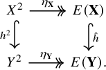
Corollary 1.4. Let $\mathbf {X}$ and $\mathbf {Y}$ be two echeloned spaces. Then, $h \colon \mathbf {X} \to \mathbf {Y}$ is an embedding if and only if there exists an embedding of ordered sets $\hat {h} \colon E(\mathbf {X}) \hookrightarrow E(\mathbf {Y})$ for which $\hat {h} \circ \eta _{\mathbf {X}} = \eta _{\mathbf {Y}} \circ h^2$ ; that is, the diagram below commutes:

Proof. ‘ $\Rightarrow $ ’: Assume h is an embedding from $\mathbf {X}$ to $\mathbf {Y}$ . Then by Lemma 1.3, there exists such a homomorphism $\hat {h} \colon E(\mathbf {X}) \to E(\mathbf {Y})$ for which $\hat {h} \circ \eta _{\mathbf {X}} = \eta _{\mathbf {Y}} \circ h^2$ . In order to prove that it does not only preserve, but also reflects $\leqslant _{E(\mathbf {X})}$ , take any $x_1, x_2, x_1^{\prime }, x_2^{\prime } \in X$ such that $\hat {h}([(x_1, x_2)]_{\sim _{\mathbf {X}}}) \leqslant _{E(\mathbf {Y})} \hat {h}([(x_1^{\prime }, x_2^{\prime })]_{\sim _{\mathbf {X}}})$ . Put differently,

$$\begin{align*}\eta_{\mathbf{Y}} \circ h^2 (x_1, x_2) = \hat{h} \circ \eta_{\mathbf{X}} (x_1, x_2) \leqslant_{E(\mathbf{Y})} \hat{h} \circ \eta_{\mathbf{X}} (x_1^{\prime}, x_2^{\prime}) = \eta_{\mathbf{Y}} \circ h^2 (x_1^{\prime}, x_2^{\prime}), \end{align*}$$

that is, $[(h(x_1), h(x_2))]_{\sim _{\mathbf {Y}}} \leqslant _{E(\mathbf {Y})} [(h(x_1^{\prime }), h(x_2^{\prime }))]_{\sim _{\mathbf {Y}}}$ . By definition of $\leqslant _{E(\mathbf {Y})}$ , we actually get $(h(x_1), h(x_2)) \leqslant _{\mathbf {Y}} (h(x_1^{\prime }), h(x_2^{\prime }))$ . Finally, as h reflects $\leqslant _{\mathbf {X}}$ , then $(x_1, x_2) \leqslant _{\mathbf {X}} (x_1^{\prime }, x_2^{\prime })$ , which is what we wanted. What remains is to show that $\hat {h}$ is injective. Take any $x_1, x_2, x_1^{\prime }, x_2^{\prime } \in X$ such that $\hat {h}([(x_1, x_2)]_{\sim _{\mathbf {X}}}) = \hat {h}([(x_1^{\prime }, x_2^{\prime })]_{\sim _{\mathbf {X}}})$ . Similarly as before, by the commutativity of the diagram, we get that $(h(x_1), h(x_2)) = (h(x_1^{\prime }), h(x_2^{\prime }))$ . As h itself is injective, it follows immediately that $(x_1, x_2) = (x_1^{\prime }, x_2^{\prime })$ .

‘ $\Leftarrow $ ’: Let $h \colon X \to Y$ be a map and assume the existence of such an $\hat {h}$ as described in the statement of the right-hand side of the corollary. First, by Lemma 1.3, we get that h is a homomorphism from $\mathbf {X}$ to $\mathbf {Y}$ . Then, take any $x_1, x_2, x_1^{\prime }, x_2^{\prime } \in X$ for which $(h(x_1), h(x_2)) \leqslant _{\mathbf {Y}} (h(x_1^{\prime }), h(x_2^{\prime }))$ . Notice how this leads to $[(h(x_1), h(x_2))]_{\sim _{\mathbf {Y}}} \leqslant _{E(\mathbf {Y})} [(h(x_1^{\prime }), h(x_2^{\prime }))]_{\sim _{\mathbf {Y}}}$ , which in turn translates to

$$\begin{align*}\hat{h} \circ \eta_{\mathbf{X}} (x_1, x_2) = \eta_{\mathbf{Y}} \circ h^2 (x_1, x_2) \leqslant_{E(\mathbf{Y})} \eta_{\mathbf{Y}} \circ h^2 (x_1^{\prime}, x_2^{\prime}) = \hat{h} \circ \eta_{\mathbf{X}} (x_1^{\prime}, x_2^{\prime}), \end{align*}$$

that is, $[(x_1, x_2)]_{\sim _{\mathbf {X}}} \leqslant _{E(\mathbf {X})} [(x_1^{\prime }, x_2^{\prime })]_{\sim _{\mathbf {X}}}$ . Thus, $(x_1, x_2) \leqslant _{\mathbf {X}} (x_1^{\prime }, x_2^{\prime })$ . Lastly, we show that h is injective. Take any $x_1, x_2 \in X$ , for which $h(x_1) = h(x_2)$ . Then $(h(x_1), h(x_2)) = (h(x_2), h(x_2))$ , and so

$$\begin{align*}\hat{h}([(x_1, x_2)]_{\sim_{\mathbf{X}}}) = \eta_{\mathbf{Y}} (h(x_1), h(x_2)) = \eta_{\mathbf{Y}} (h(x_2), h(x_2)) = \hat{h}([(x_2, x_2)]_{\sim_{\mathbf{X}}}). \end{align*}$$

As a result of $\hat {h}$ being injective, we get that $(x_1, x_2) \sim _{\mathbf {X}} (x_2, x_2)$ . However, by the axioms of an echeloned space, this leads to $x_1 = x_2$ . This concludes the proof.

As the next lemma shows, every metric space induces an echeloned space on the same set of points.

Lemma 1.5. Let $(M, d_M)$ be a metric space. Define a binary relation $\leqslant _{\mathbf {M}}$ on $M^2$ such that for every $(x_1, y_1), (x_2, y_2) \in M^2$ ,

$$\begin{align*}(x_1, y_1) \leqslant_{\mathbf{M}} (x_2, y_2) \quad \Longleftrightarrow \quad d_M(x_1, y_1) \leqslant d_M(x_2, y_2).\end{align*}$$

Then $(M, \leqslant _{\mathbf {M}})$ is an echeloned space.

Proof. We proceed to prove that $\leqslant _{\mathbf {M}}$ is an echelon on M. As $\leqslant $ is a linear order on $\mathbb {R}$ , $\leqslant _{\mathbf {M}}$ is trivially a prechain on $M^2$ by its definition. For any $x, y, z \in M$ ,

1. (i) $d_M(x,x) = 0 \leqslant d_M(y, z)$ ; thus, $(x,x) \leqslant _{\mathbf {M}} (y, z)$ .

2. (ii) if $(y, z) \leqslant _{\mathbf {M}} (x, x)$ , then $d_M(y, z) \leqslant d_M(x, x) = 0$ . So $d_M(y, z) = 0$ , and so $y = z$ .

3. (iii) $d_M(x, y) = d_M(y, x)$ , so $(x, y) \leqslant _{\mathbf {M}} (y, x)$ .

Remark 1.6. By Lemma 1.3, two metric spaces $(X, d_X)$ and $(Y, d_Y)$ are isomorphic as echeloned spaces if and only if there exist a bijection $f\colon X \to Y$ and an automorphism $\hat {f}$ of $(\mathbb {R}^+, <)$ such that $d_Y (f(x), f(x'))$ = $\hat {f} (d_X (x, x'))$ for all $x, x' \in X$ . This kind of equivalence relation between metric spaces has been considered by several authors; see, for example, [10] and the references therein.

Remark 1.7. The proof of Lemma 1.5 does not make use of the triangle inequality. Thus, the statement remains true if $(M, d_M)$ is merely a semimetric space. This was already noted in [16, Example 1.4].

Obviously, not every echeloned space is induced by a metric space in this way. A necessary condition for $\mathbf {X}$ to be induced by a metric space is that $E(\mathbf {X})$ embeds into the chain of reals; see Examples 1.13 and 1.14. The question when a linear order can be embedded into the chain of reals was settled by Birkhoff. Recall that a subset S of a prechain $(C,\leqslant )$ is called order-dense in C if and only if, for every $a < b$ in $C\setminus S$ , there exists $s\in S$ such that $a \le s \le b$ .

Theorem 1.8 [2, Theorem VIII.24]²

A linearly ordered set embeds into $(\mathbb {R},\le )$ if and only if it contains a countable order-dense subset.

Definition 1.9. A metric space $(X, d_X)$ is called dull if $d_X(x,x') \leqslant d_X(y,y') + d_X(z, z')$ holds, for all $x, x', y, y', z, z' \in X$ with $y \not = y'$ and $z \not = z'$ .

Recall that a metric space is called uniformly discrete if all nonzero distances in it are bounded from below by some constant $c>0$ .

Lemma 1.10. Any dull metric space is both bounded and uniformly discrete.

Proof. Let $(X, d_X)$ be a dull metric space. Define . Clearly, the diameter of $(X,d_X)$ is not larger than $2 \tau $ , due to dullness. Thus, any distance within $(X, d_X)$ is bounded by $2 \tau $ .

Without loss of generality, assume $|X| \not = 1$ . In other words, there exist such $x, y \in X$ that $d_X(x, y) \not = 0$ . As $\tau \leqslant d_X(x, y) \leqslant 2 \tau $ , it follows that $\tau> 0$ . Consequently, as $0 < \tau \leqslant d_X(x, y)$ for all distinct $x, y \in X$ , $(X, d_X)$ is uniformly discrete.

Proposition 1.11 (cf. [16, Proposition 1.5])

Let $(X,\leqslant _{\mathbf {X}})$ be an echeloned space. Then the following are equivalent:

1. (i) $\leqslant _{\mathbf {X}}$ is induced by a metric space,

2. (ii) $\leqslant _{\mathbf {X}}$ is induced by a dull metric space,

3. (iii) $(X^2,\leqslant _{\mathbf {X}})$ contains a countable order-dense subset,

4. (iv) $E(\mathbf {X})$ embeds into $(\mathbb {R},\le )$ .

Proof. We show $(ii)\Rightarrow (i)\Rightarrow (iv)\Rightarrow (ii)$ , and $(iii)\iff (iv)$ . It is clear that $(ii)\Rightarrow (i)$ .

‘ $(i)\Rightarrow (iv)$ ’: Let X be a set and $\leqslant _{\mathbf {X}}$ an echelon on it induced by a metric space $(X, d_X)$ . Clearly, $\operatorname {\mathrm {im}} d_X$ is order-embeddable into the reals, given that $d_X$ is a metric. Observe that $E(\mathbf {X}) \cong (\operatorname {\mathrm {im}} d_X, \leqslant )$ .

‘ $(iv)\Rightarrow (ii)$ ’: Let f be an embedding of $E(\mathbf {X})$ into $(\mathbb {R},\le )$ . Without loss of generality, we may assume that the image of f is contained in $(\{0\} \cup (1, 2), \leqslant )$ , and that f maps the smallest element of $E(\mathbf {X})$ (containing all reflexive pairs) to $0$ .

Now we define a map $d_X$ on $X^2$ as follows: for any $(x, y) \in X^2$ , let . It remains to show that it is a well-defined metric.

To begin with, notice that for any $x \in X$ , the distance $d_X(x, x) = f ([(x,x)]_{\sim _{\mathbf {X}}}) = 0$ . For any $x, y \in X$ , $d_X (x, y) \geqslant 0$ . Also, since $(x, y) \sim _{\mathbf {X}} (y, x)$ , then $d_X (x, y) = d_X (y, x)$ . At last, take any $x, y, z \in X$ . If x, y, and z are pairwise distinct, then

$$\begin{align*}d_X(x, y) = f([(x, y)]_{\sim_{\mathbf{X}}}) < 2 = 1 + 1 < f([(x, z)]_{\sim_{\mathbf{X}}}) + f([(z, y)]_{\sim_{\mathbf{X}}}) = d_X(x, z) + d_X(z, y).\end{align*}$$

Otherwise, if $x=y$ , then $d_X(x, y) = 0 \leqslant d_X(x, z) + d_X(z, y)$ ; whereas if $x=z$ or $y=z$ , then the triangle inequality trivially holds.

Overall, $(X, d_X)$ is indeed a metric space (inducing the echeloned space $(X, \leqslant _{\mathbf {X}})$ ). Moreover, by definition, it is dull.

‘ $(iii)\Rightarrow (iv)$ ’: Let S be a countable order-dense subset of $X^2$ . Consider

Clearly, $S_{E(\mathbf {X})}$ is a countable order-dense subset of $E(\mathbf {X})$ . By Theorem 1.8, $E(\mathbf {X})$ embeds into $(\mathbb {R},\le )$ .

‘ $(iv)\Rightarrow (iii)$ ’: By Theorem 1.8, $E(\mathbf {X})$ contains a countable order-dense subset $S_{E(\mathbf {X})}$ . Let T be a transversal of $\sim _{\mathbf {X}}$ . Consider

Then it is easy to see that S is countable and order-dense in $(X^2,\le _{\mathbf {X}})$ .

An echeloned space that is induced by a metric space will be called metrizable. As a direct consequence of Proposition 1.11 we obtain the following:

Corollary 1.12. Every echeloned space on a countable set is metrizable.

What follows are two examples of non-metrizable echeloned spaces.

Example 1.13. Observe the following chain $C = \mathbb {R}_0^+ \odot \mathbf {2}$ , where $\mathbb {R}_0^+$ is the set of nonnegative real numbers, and where $\mathbf {2} = \{0,1\}$ is the ordinal number 2. Recall that the lexicographic product $X \odot Y$ , of two disjoint posets X and Y, is the set of all ordered pairs $(x, y)$ (where $x \in X, y \in Y$ ), ordered lexicographically – that is, by the rule that $(x,y) < (x', y')$ if and only if $x < x'$ or $x = x' \land y < y'$ . Clearly, the lexicographic product of any two chains is again a chain. Take any countable subset S of C. As there exist uncountably many irrational numbers, there has to be some $a \in \mathbb {R}_0^+ \setminus \mathbb {Q}$ such that neither $(a, 0)$ nor $(a, 1)$ are in S. Due to the lexicographical ordering, there is no element of C, let alone of S, in between the formerly mentioned two. Therefore, S cannot be order-dense in C. Since the choice of S was arbitrary, by [2, Theorem VIII.24], C is not embeddable into $\mathbb {R}$ .

Now, consider an echelon $\leqslant _{\mathbb {R}}$ on the set of reals defined as follows:

$$ \begin{align*} (x,y) <_{\mathbb{R}} (u,v) \quad :\Longleftrightarrow \quad &\text{ either } \bigl||x|-|y|\bigr| < \bigl||u|-|v|\bigr|,\\ &\text{ or } \bigl||x|-|y|\bigr| = \bigl||u|-|v|\bigr|, \text{ but }\operatorname{\mathrm{sgn}}(x) = \operatorname{\mathrm{sgn}}(y),\, \operatorname{\mathrm{sgn}}(u) \not= \operatorname{\mathrm{sgn}}(v), \end{align*} $$

for any $(x, y), (u, v) \in \mathbb {R}^2$ . Observe that the chain $({\mathbb {R}^2}/{\sim _{\mathbb {R}}}, \leqslant _{\mathbb {R}})$ is isomorphic to $(\mathbb {R}^+_0 \odot \mathbf {2}, \leqslant )$ . As a result of Proposition 1.11, the latter echelon could not have been induced by a metric space.

Example 1.14. Let . Further, we define a map $f_{\mathbf {X}} \colon X^2 \to \omega _1^+$ as follows. Let $\mathbf {x} = (x_i)_{i \in \omega _1}$ , $\mathbf {y} = (y_i)_{i \in \omega _1} \in X$ . Then if $\mathbf {x} \not = \mathbf {y}$ , we set , where k is the smallest index for which $x_k \not = y_k$ ; otherwise, . Moreover, we define a binary relation $\leqslant _{\mathbf {X}}$ on $X^2$ so that

$$\begin{align*}(\mathbf{x}, \mathbf{y}) \leqslant_{\mathbf{X}} (\mathbf{s}, \mathbf{t}) \quad :\Longleftrightarrow\quad f_{\mathbf{X}}(\mathbf{x}, \mathbf{y}) \geqslant f_{\mathbf{X}}(\mathbf{s}, \mathbf{t}).\end{align*}$$

Clearly, $\leqslant _{\mathbf {X}}$ is a well-defined echelon on X. Given that $f_{\mathbf {X}}$ is surjective, the chain $\left ({X^2}/{\sim _{\mathbf {X}}}, \leqslant _{\mathbf {X}}~\!\right )$ is isomorphic to $(\omega _1^+, \geqslant )$ . As already $\omega _1$ does not order-embed into the reals,³ neither does $\omega _1^+$ . By [2, Theorem VIII.24], $(\omega _1^+, \geqslant )$ does not have a countable order-dense subset. Consequently, by Proposition 1.11, the echelon $\leqslant _{\mathbf {X}}$ is not induced by a metric space.

We have already provided a full characterisation of metrizable echeloned spaces; cf. Proposition 1.11.

For any two metric spaces $\mathcal {M} = (M, d_M)$ and $\mathcal {N} = (N, d_N)$ , we define $\operatorname {\mathrm {Hom}}(\mathcal {M}, \mathcal {N})$ as the set of all $1$ -Lipschitz maps from $\mathcal {M}$ to $\mathcal {N}$ . Note that not every homomorphism between metric spaces is at the same time a homomorphism between the echeloned spaces induced by them; cf. Example 1.16.

Let $\operatorname {\mathrm {Lip}}^{\leqslant }_1(\mathcal {M}, \mathcal {N})$ denote the set of all 1-Lipschitz maps between the metric spaces $\mathcal {M}$ and $\mathcal {N}$ that preserve the echelon relations of $\mathcal {M}$ and $\mathcal {N}$ .

Proposition 1.15. Let $\mathbf {M} = (M, \leqslant _{\mathbf {M}})$ and $\mathbf {N} = (N, \leqslant _{\mathbf {N}})$ be two metrizable echeloned spaces. Then, there exist metric spaces, $\mathcal {M}$ and $\mathcal {N}$ , that induce $\mathbf {M}$ and $\mathbf {N}$ , respectively, and for which

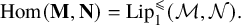$$\begin{align*}\operatorname{\mathrm{Hom}}(\mathbf{M}, \mathbf{N}) = \operatorname{\mathrm{Lip}}^{\leqslant}_1(\mathcal{M}, \mathcal{N}).\end{align*}$$

Proof. The proof of Proposition 1.11 provides us with the existence of dull metrics $d_M$ and $d_N$ on M and N which induce the echelons $\leqslant _{\mathbf {M}}$ and $\leqslant _{\mathbf {N}}$ . By rescaling $d_M$ , we may assume that $\operatorname {\mathrm {im}} d_M \subseteq \{0\} \cup (2, 4)$ and that $\operatorname {\mathrm {im}} d_N \subseteq \{0\} \cup (1,2)$ . Now, take any $f \in \operatorname {\mathrm {Hom}}(\mathbf {M}, \mathbf {N})$ . As for any two distinct $x, y \in M$ ,

$$\begin{align*}d_N (f(x), f(y)) < 2 < d_M (x,y),\end{align*}$$

f is trivially a $1$ -Lipschitz map between the metric spaces $\mathcal {M}$ and $\mathcal {N}$ . Therefore, $f\in \operatorname {\mathrm {Lip}}^{\leqslant }_1(\mathcal {M}, \mathcal {N})$ . The reverse inclusion holds trivially.

Already for finite echeloned spaces, there are $1$ -Lipschitz maps that do not preserve the echelons, as can be seen from the example below.

Example 1.16. Consider the metric spaces $\mathcal {M}$ and $\mathcal {N}$ , given by $M = \{x_1, x_2, x_3\}$ and $N = \{y_1, y_2, y_3\}$ , and the metrics $d_M$ and $d_N$ such that

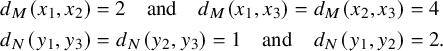$$ \begin{align*} d_M(x_1, x_2) &= 2 \quad \text{and} \quad d_M (x_1, x_3) = d_M (x_2, x_3) = 4\\ d_N(y_1, y_3) &= d_N (y_2, y_3) = 1 \quad \text{and} \quad d_N(y_1, y_2) = 2.\\[-48pt] \end{align*} $$

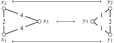
Any map $f\colon \mathcal {M}\to \mathcal {N}$ is $1$ -Lipschitz, but there are maps that do not preserve echelons – for instance, $f\colon x_i\mapsto y_i$ .

Proposition 1.17. Let $\mathbf {X}$ be an echeloned space with $E(\mathbf {X})$ well-ordered. If f is an automorphism of $\mathbf {X}$ , then $\hat {f}\colon E(\mathbf {X})\to E(\mathbf {X})$ is the identity embedding.

Proof. Let f be an automorphism of $\mathbf {X}$ . As a consequence of Corollary 1.4, $\hat {f}$ is an automorphism of the echeloning $E(\mathbf {X})$ . Since $E(\mathbf {X})$ is well-ordered, a standard induction argument shows that $\hat {f}=\mathrm {id}_{E(\mathbf {X})}$ .

Corollary 1.18. Let $(X, d_X)$ be a metric space with $(d_X[X^2], \leqslant )$ well-ordered. Then the automorphism group of the induced echeloned space is the same as its isometry group, i.e. $\operatorname {\mathrm {Aut}}(X, \leqslant _{\mathbf {X}}) = \operatorname {\mathrm {Iso}}(X, d_X)$ .

Proof. This follows immediately from Proposition 1.17 and Corollary 1.4.

Corollary 1.19. Let $\mathbf {X}$ be a finite echeloned space induced by a metric space $(X, d_X)$ . Then $\operatorname {\mathrm {Aut}}(\mathbf {X}) = \operatorname {\mathrm {Iso}}(X, d_X)$ .

Proof. Since every finite linear order is a well-order, this follows immediately from Corollary 1.18.

Despite Corollaries 1.18 and 1.19, we shall see in Section 3 that the Fraïssé limit of the class of all finite echeloned spaces is not induced by the Fraïssé limit of the class of all finite rational metric spaces – namely, the rational Urysohn metric space.

2 Echeloned structure of metric spaces

In this section, we take a little detour by studying the echeloned structure of some nicely behaved metric spaces. We start by showing that under some mild restriction, homomorphisms are uniformly continuous.

Proposition 2.1. Let $(X, d_X)$ and $(Y, d_Y)$ be metric spaces inducing echelons $\leqslant _{\mathbf {X}}$ and $\leqslant _{\mathbf {Y}}$ , respectively. Let $f \colon (X, \leqslant _{\mathbf {X}}) \to (Y, \leqslant _{\mathbf {Y}})$ be such a homomorphism for which the metric space $(f[X], d_Y \mathord {\upharpoonright }_{f[X]})$ is not uniformly discrete. Then, f is uniformly continuous.

Proof. Let $\varepsilon> 0$ . Without loss of generality, assume $|X|> 1$ . As $(f[X], d_Y \mathord {\upharpoonright }_{f[X]})$ is not uniformly discrete, there exist $x_0, y_0 \in X$ such that $0 \not = d_Y(f(x_0), f(y_0)) \leqslant \varepsilon $ . Note that . We will show that for any $x, y \in X$ for which $d_X(x, y) < \delta $ , it follows that $d_Y(f(x), f(y)) < \varepsilon $ .

Thus, take any $x, y \in X$ , such that $d_X(x, y) < d_X(x_0, y_0)$ . The latter is equivalent to $(x, y) <_{\mathbf {X}} (x_0, y_0)$ . As f is a homomorphism between the induced echeloned spaces, $(f(x), f(y)) <_{\mathbf {Y}} (f(x_0), f(y_0))$ , which in turn is equivalent to

$$\begin{align*}d_Y((f(x), f(y))) < d_Y(f(x_0), f(y_0)) \leqslant \varepsilon.\\[-34pt] \end{align*}$$

Corollary 2.2. Let $(X, d_X)$ be a metric space inducing the echelon $\leqslant _{\mathbf {X}}$ . Then any automorphism of $(X, \leqslant _{\mathbf {X}})$ is uniformly continuous.

Proof. If $(X, d_X)$ is not uniformly discrete, we obtain the claim by Proposition 2.1. Otherwise, the statement is trivial.

The corollary above implies that the isometry group of a metric space $(X, d_X)$ is a subgroup of the automorphism group of the echeloned space $(X, \leqslant _{\mathbf {X}})$ , which in turn is a subgroup of the automorphism group of the uniformity space induced by $(X, d_X)$ .

The example below shows that homomorphisms between echeloned spaces need not to be uniformly continuous, even if the echeloned spaces in question are induced by metric spaces.

Example 2.3. Let be endowed with the usual metric. Let be endowed with the ${\ell }^{1}$ metric (where $\delta _i$ denotes the sequence with all entries $0$ , except for the i ^th which is $1$ ). Then the map $f \colon X \to Y$ defined so as to map $0$ to $\delta _{-1}+\delta _0$ and $\frac {1}{n}$ to $\left (1 + \frac {1}{n}\right ) \delta _0 + \delta _n$ is bijective and also preserves the echelon induced by the metric since $d_Y(f(x),f(x'))=d_X(x,x')+2$ , for every $x\neq x'$ . However, it is not continuous, let alone uniformly continuous.

Recall that a metric space is called Cantor-connected if for all $\varepsilon>0$ and any two points x and y, there exist $n\ge 0$ and a sequence $x_0,\dots , x_n$ such that $x_0=x$ , $x_n=y$ , and $d(x_i,x_{i+1})\le \varepsilon $ , for all $0\le i <n$ (such a sequence is called an $\varepsilon $ -chain from x to y). The following observation provides an interesting dichotomy for homomorphisms between echeloned spaces whose domain is induced by a Cantor-connected metric space:

Observation 2.4. Let $(Y,\le _{\mathbf {Y}})$ be an echeloned space and let $(X, d_X)$ be a metric space inducing the echelon $\leqslant _{\mathbf {X}}$ . Let $f \colon (X, \leqslant _{\mathbf {X}}) \to (Y, \leqslant _{\mathbf {Y}})$ be a homomorphism. If $(X, d_X)$ is Cantor-connected, then f is constant or injective.

Proof. Assume f is not injective. That means that there exist distinct $x_0, y_0 \in X$ such that $f(x_0) = f(y_0)$ . Let . Take any $x, y \in X$ and let $x=m_0,m_1, m_2, \dots , m_n=y$ be an $\varepsilon $ -chain from x to y. Consequently, for all $i \in \{0, 1, \dots , n-1\}$ , we have $(m_i, m_{i+1}) \leqslant _{\mathbf {X}} (x_0, y_0)$ . Since f is a homomorphism, it follows that $(f(m_i), f(m_{i+1})) \leqslant _{\mathbf {Y}} (f(x_0), f(y_0)) = (f(x_0), f(x_0))$ . Thus, $f(m_i) = f(m_{i+1})$ for all $i \in \{0, 1, \dots , n-1\}$ , leading to $f(x) = f(y)$ . From the arbitrary choice of x and y, we conclude that f is constant.

We turn our attention to a class of Cantor-connected metric spaces for which the automorphisms of the induced echelon are exactly the dilations; see Proposition 2.8.

Definition 2.5. Let $(X, d_X)$ be a metric space. A point $z \in X$ is called a midpoint of x and y, where $x, y \in X$ , if

$$\begin{align*}d_X(z, x) = d_X(z, y) = \frac{1}{2}d_X(x, y).\end{align*}$$

The set of all midpoints of points $x, y \in X$ is denoted by $\operatorname {\mathrm {Mid}}_X(x, y)$ . The metric space itself is said to have midpoints if for any $x, y \in X$ , there exists a midpoint of x and y.

Lemma 2.6. Let $(X, d_X)$ and $(Y, d_Y)$ be metric spaces inducing echelons $\leqslant _{\mathbf {X}}$ and $\leqslant _{\mathbf {Y}}$ , respectively. Let $f \colon (X, \leqslant _{\mathbf {X}}) \to (Y, \leqslant _{\mathbf {Y}})$ be a surjective homomorphism. If $(X, d_X)$ and $(Y, d_Y)$ have midpoints, then for all $x, y \in X$ ,

$$\begin{align*}f\left[\operatorname{\mathrm{Mid}}_X(x, y)\right] \subseteq \operatorname{\mathrm{Mid}}_Y(f(x), f(y)).\end{align*}$$

Proof. Take any $x, y \in X$ and denote by m a midpoint of x and y. Then we have that $d_X(x, m) = d_X(m, y) = \frac {1}{2} d_X(x, y)$ . Thus, $(x, m) \sim _{\mathbf {X}} (m, y)$ , and so $(f(x), f(m)) \sim _{\mathbf {Y}} (f(m), f(y))$ ; that is, $d_Y(f(x), f(m)) = d_Y(f(m), f(y))$ . Now, from the triangle inequality, we know that $d_Y(f(x), f(y)) \leqslant d_Y(f(x), f(m)) + d_Y(f(m), f(y)) = 2 d_Y(f(x), f(m))$ . Hence, $\frac {1}{2} d_Y(f(x), f(y)) \leqslant d_Y(f(x), f(m))$ .

In what follows, we shall show that $f(m)$ is in fact a midpoint of $f(x)$ and $f(y)$ . As $(Y,d_Y)$ has midpoints and f is surjective, there exists $m'\in X$ such that $f(m')\in \operatorname {\mathrm {Mid}}(f(x),f(y))$ . Next, we show that

$$\begin{align*}d_Y(f(x),f(m)) \le d_Y(f(x),f(m'))=\tfrac{1}{2} d_Y(f(x),f(y)). \end{align*}$$

Without loss of generality, we may assume that $d_X(x,m')\le d_X(m',y)$ . Then $d_X(m,y)=d_X(x,m)\le d_X(m',y)$ since

$$\begin{align*}2d_X(x,m)= d_X(x,y)\le d_X(x,m')+d_X(m',y)\le 2 d_X(m',y). \end{align*}$$

Now, in case that $d_X(x,m)\le d_X(x,m')$ , we have that $d_Y(f(x),f(m))\le d_Y(f(x),f(m'))$ . If, on the other hand, $d_X(x,m')\le d_X(x,m)$ , then

$$ \begin{align*} d_Y(f(x),f(m')) \le d_Y(f(x),f(m))\le d_Y(f(m'),f(y)) = d_Y(f(x),f(m')). \end{align*} $$

In both cases, we arrive at the conclusion that $f(m)\in \operatorname {\mathrm {Mid}}(f(x),f(y))$ , as desired.

Remark 2.7. Let $(X,d_X)$ be a metric space. Recall that a triple $(a,b,c)\in X^3$ is said to be collinear if

$$\begin{align*}d_X(a,b)+d_X(b,c) = d_X(a,c). \end{align*}$$

Furthermore, it is well known and easy to see that for any four points $a,b,c,d\in X$ , joint collinearity of $(a,b,d)$ and $(b,c,d)$ implies the collinearity of $(a,b,c)$ and of $(a,c,d)$ (see [19, Section 2]; cf. [6, Section 6]).

Proposition 2.8. Let f be an automorphism of the echeloned space $(X, \leqslant _{\mathbf {X}})$ , induced by a metric space $(X, d_X)$ that has midpoints. Then f is a dilation; that is, there exists a positive real number t such that for all $x, y \in X$ , we have that $d_X(f(x), f(y)) = t \cdot d_X(x, y)$ .

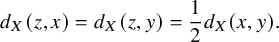
Proof. Let $\hat {f}$ be the action of f on the echeloning of $(X, \leqslant _{\mathbf {X}})$ (cf. Corollary 1.4). Define $\tilde {d}_X \colon E(X)\to \operatorname {\mathrm {im}} d_X,\, [(x,y)]_{\sim _{\mathbf {X}}}\mapsto d_X(x,y)$ . Since $\leqslant _{\mathbf {X}}$ is induced by $d_X$ , it is easy to see that $\tilde {d}_X$ is an order isomorphism (cf. Lemma 1.5). Let . In particular, for all $a,b\in X$ , we have $\tilde {f}(d_X (a,b))=d_X (f(a),f(b))$ , and the following diagram commutes:

We will show that for every $\delta \in \operatorname {\mathrm {im}} d_X\setminus \{0\}$ , the restriction of $\tilde {f}$ to the initial segment is linear. Since, for any $0 < \delta < \delta ' \in \operatorname {\mathrm {im}} d_X$ , we have $\{0\} \neq I(\delta ) \subseteq I(\delta ')$ , it will follow that $\tilde {f}$ as a whole is linear; that is, f is a dilation.

Let . Let $a, c \in X$ with $ d_X(a, c) = \delta $ , and therefore with $t = \tfrac { d_X (f(a), f(c))}{ d_X (a, c)}$ . Let b be a midpoint of a and c.

Let $s\in I(\delta )$ . Since $\tilde {f}(0)=0=t\cdot 0$ , we may and will assume that $s\neq 0$ . We choose recursively a sequence $(b_n,c_n)_{n\in \mathbb {N}}$ in $X^2$ with

$$\begin{align*}\forall n\in\mathbb{N}\,:\, s\le d_X(a,c_n), \text{ and } (a,b_n,c_n) \text{ is collinear.} \end{align*}$$

We proceed as follows: . If $(b_n,c_n)$ has been chosen, then $(b_{n+1},c_{n+1})$ is chosen according to the following cases:

Case 1: if $s=d_X(a,c_n)$ , then put ,

Case 2: if $d_X(a,b_n)<s<d_X(a,c_n)$ , then choose $m\in \operatorname {\mathrm {Mid}}(b_n,c_n)$ and put

Case 3: if $d_X(a,b_n)=s$ , then put ,

Case 4: if $0< s < d_X(a,b_n),$ then choose $m\in \operatorname {\mathrm {Mid}}(a,b_n)$ and put .

Let us call a pair $(x,y)\in X^2$ homothetic if

1. 1) $(a,x,y)$ is collinear,

2. 2) $(f(a),f(x),f(y))$ is collinear,

3. 3) $d_X(f(a),f(x))=t\cdot d_X(a,x),\quad d_X(f(x),f(y)) = t\cdot d_X(x,y)$ .

A straightforward induction using Remark 2.7 and Lemma 2.6 shows that for every $n\in \mathbb {N}$ , the pair $(b_n,c_n)$ is homothetic. Furthermore,

$$\begin{align*}s = \lim_{n\to\infty} d_X(a,b_n) = \lim_{n\to\infty} d_X(a,c_n). \end{align*}$$

Note that since $s>0$ , for all but finitely many n, we have $d_X(a,b_n)\le s$ .

Since $\tilde {f}(d_X(a,b_n)) = t\cdot d_X(a,b_n)$ and $\tilde {f}(d_X(a,c_n)) = t\cdot d_X(a,c_n)$ for all $n\in \mathbb {N}$ , monotonicity of $\tilde {f}$ implies that $\tilde {f}(s)=t\cdot s$ , as desired.

What follows is an example of a metric space and an automorphism of the induced echeloned space which is not a dilation.

Example 2.9. We define a subspace X of the Euclidean line $\mathbb {R}$ as follows. Let $a> 2$ and $0 < \varepsilon < \tfrac {a}{2} - 1$ . Let $x_0 = 1 + \varepsilon $ and, for any $k \in \mathbb {Z} \setminus \{0\}$ , $x_k = a^k$ . Let finally $X = \{x_k\mid k \in \mathbb {Z}\}$ be endowed with the usual Euclidean metric. Observe that X does not have midpoints since it is discrete.

We claim that the shift $\sigma \colon X \rightarrow X,\, x_k \mapsto x_{k + 1}$ is an automorphism of the echelon relation $\leqslant _{\mathbf {X}}$ of X. Obviously, $\sigma $ is not a dilation, since $\varepsilon \neq 0$ .

To check that it is indeed an automorphism, let us consider two distinct pairs of distinct points $\{x_k, x_\ell \}$ and $\{x_{k'}, x_{\ell '}\}$ . We may assume without loss of generality that $k> \ell $ and $k'> \ell '$ , and moreover, $k \geqslant k'$ . Two cases are to be considered:

1. (i) If $k = k'$ , then $(x_{k'}, x_{\ell '}) \leqslant _{\mathbf {X}} (x_k, x_\ell )$ if and only if $\ell \leqslant \ell '$ . This is obviously equivalent to $k + 1 = k' + 1$ and $\ell + 1 \leqslant \ell ' + 1$ , that is, to $(\sigma (x_{k'}), \sigma (x_{\ell '})) \leqslant _{\mathbf {X}} (\sigma (x_k), \sigma (x_\ell ))$ .

2. (ii) If $k> k'$ , then necessarily $(x_{k'}, x_{\ell '}) < (x_k, x_\ell )$ . Indeed, we have

   $$ \begin{align*} d_X (x_k, x_\ell) \geqslant d_X (x_k, x_{k - 1}) &= \begin{cases} a^{k - 1} (a - 1) & \text{if } k \neq 1, \\ a - 1 - \varepsilon & \text{if } k = 1, \end{cases} \\d_X (x_{k'}, x_{\ell'}) \leqslant x_{k'} \leqslant x_{k - 1} &= \begin{cases} a^{k - 1} & \text{if } k \neq 1, \\ 1 + \varepsilon & \text{if } k = 1. \end{cases} \end{align*} $$
   And therefore, $ d_X (x_k, x_\ell )> d_X (x_{k'}, x_{\ell '})$ whatever k, thanks to our choice of $\varepsilon $ and a. Since obviously $k + 1> k' + 1$ , the same argument would hold for the images by the shift; that is, $(\sigma (x_{k'}), \sigma (x_{\ell '})) <_{\mathbf {X}} (\sigma (x_k), \sigma (x_\ell ))$ .

3 The Fraïssé limit of the class of finite echeloned spaces

We now turn our attention to the proof of the existence of a countable universal homogeneous echeloned space.

Proposition 3.1. The class of finite echeloned spaces has the amalgamation property.

Proof. Consider any three finite echeloned spaces $\mathbf {A}, \mathbf {B}_1, \mathbf {B}_2$ together with embeddings $f_1 \colon \mathbf {A} \hookrightarrow \mathbf {B}_1$ and $f_2 \colon \mathbf {A} \hookrightarrow \mathbf {B}_2$ . By Corollary 1.4, we obtain embeddings $\hat {f}_1 \colon E(\mathbf {A}) \hookrightarrow E(\mathbf {B}_1)$ and $\hat {f}_2 \colon E(\mathbf {A}) \hookrightarrow E(\mathbf {B}_2)$ , for which the following equations hold:

$$\begin{align*}\hat{f_1} \circ \eta_{\mathbf{A}} = \eta_{\mathbf{B}_1} \circ {f_1}^2 \quad \text{and} \quad \hat{f_2} \circ \eta_{\mathbf{A}} = \eta_{\mathbf{B}_2} \circ {f_2}^2.\end{align*}$$

Notice that $E(\mathbf {A})$ , $E(\mathbf {B}_1)$ and $E(\mathbf {B}_2)$ are all (finite) linear orders. Given that the class of finite linear orders has the amalgamation property, there exist a linear order $(D, \sqsubseteq )$ and embeddings

$$\begin{align*}{g}_1 \colon E(\mathbf{B}_1) \hookrightarrow (D, \sqsubseteq) \quad \text{and} \quad {g}_2 \colon E(\mathbf{B}_2) \hookrightarrow (D, \sqsubseteq)\end{align*}$$

for which ${g}_1 \circ \hat {f}_1 = {g}_2 \circ \hat {f}_2$ , that is, for which this diagram commutes:

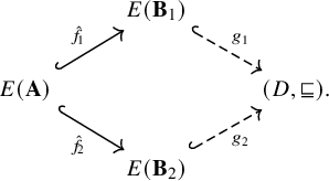
For each $i\in \{1,2\}$ , observe that $\min E(\mathbf {B}_i)=\hat {f}_i (\min E(\mathbf {A}))$ , and therefore, without loss of generality, we can assign $g_i(\min E(\mathbf {B}_i))=\min (D, \sqsubseteq )$ . Moreover, we may assume that $\min (D, \sqsubseteq )\neq \max (D, \sqsubseteq )$ . Now, define and $\eta \colon C^2 \to (D, \sqsubseteq )$ as

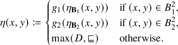
Observe that $\eta $ is well defined. Now, we define a binary relation $\leqslant _{\mathbf {C}}$ on $C^2$ as follows:

$$\begin{align*}(c_1, c_2) \leqslant_{\mathbf{C}} (c_1^{\prime}, c_2^{\prime}) \quad :\Longleftrightarrow \quad \eta(c_1, c_2) \sqsubseteq \eta(c_1^{\prime}, c_2^{\prime}).\end{align*}$$

What we need to show now is that is indeed an echeloned space. The only nontrivial point to show is axiom (ii) from Definition 1.1. Take any $c_0, c_1, c_2 \in C$ . Let us assume that $(c_1, c_2) \leqslant _{\mathbf {C}} (c_0, c_0)$ . Then $\eta (c_1, c_2) \sqsubseteq \eta (c_0, c_0) = \min (D, \sqsubseteq )$ , and so $\eta (c_1, c_2) = \min (D, \sqsubseteq )$ . In other words, $(c_1, c_2) \in \mathbf {B}_i^2$ for some $i \in \{1, 2\}$ . Therefore, axiom (ii) for $\mathbf {B}_1$ or $\mathbf {B}_2$ implies $c_1=c_2$ . Thus, $\mathbf {C}$ is a well-defined finite echeloned space.

It remains to show that the dashed arrows in the following commuting diagram are embeddings:

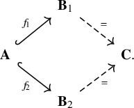
Indeed, for any choice of $b_1, b_2, b_1^{\prime }, b_2^{\prime } \in \mathbf {B}_i$ , for $i \in \{1, 2\}$ , $(b_1, b_2) \leqslant _{\mathbf {B}_i} (b_1^{\prime }, b_2^{\prime })$ is equivalent to $\eta _{\mathbf {B}_i} (b_1, b_2) \leqslant _{E(\mathbf {B}_i)} \eta _{\mathbf {B}_i} (b_1^{\prime }, b_2^{\prime })$ , which in turn is equivalent to $\eta (b_1, b_2) \sqsubseteq \eta (b_1^{\prime }, b_2^{\prime })$ , that is, to $(b_1, b_2) \leqslant _{\mathbf {C}} (b_1^{\prime }, b_2^{\prime })$ . This concludes the proof.

Remark 3.2. The proof of Proposition 3.1 actually shows that the class of finite echeloned spaces has the strong amalgamation property (in the sense of [18, page 1602]).

Proposition 3.3. The class of finite echeloned spaces is a Fraïssé class.

Proof. What we need to show is that the class of finite echeloned spaces has the hereditary property ( $\operatorname {HP}$ ), the joint embedding property ( $\operatorname {JEP}$ ) and the amalgamation property ( $\operatorname {AP}$ ), and that up to isomorphism, there exist just countably many finite echeloned spaces.

The $\operatorname {AP}$ was already established in Proposition 3.1. With regards to establishing the $\operatorname {JEP}$ , observe that, by definition, an echeloned space is defined on a nonempty set. Note that the trivial one element echeloned space is embeddable into any echeloned space. Therefore, in this case, the $\operatorname {JEP}$ follows from the $\operatorname {AP}$ . Any subset of an echeloned space induces an echeloned space. Thus, this class has the $\operatorname {HP}$ . Having been defined over a finite relational signature, it clearly has only countably many isomorphism classes.

Proposition 3.3, together with Fraïssé’s theorem, asserts the existence of a unique (up to isomorphism) countable universal homogeneous echeloned space. We will denote this Fraïssé limit by $\mathbf {F} = (F, \leqslant _{\mathbf {F}})$ and the smallest element of its echeloning by $\bot _{\mathbf {F}}$ .

We proceed by examining the structure of $\mathbf {F}$ in more detail.

Lemma 3.4. $E(\mathbf {F}) \cong (\mathbb {Q}^+_0, \leqslant )$ .

Proof. What we will show is that excluding $\bot _{\mathbf {F}}$ from the echeloning of $\mathbf {F}$ leaves us with a countable dense linear order without endpoints. In other words, the original structure is isomorphic to the set of nonnegative rational numbers equipped with the natural order.

As $\mathbf {F}$ is an echeloned space, $E(\mathbf {F})$ is a linear order. Take any $u_1, u_2, u_3, u_4 \in F$ such that $(u_1, u_2) <_{\mathbf {F}} (u_3, u_4)$ . Define and let $\mathbf {U}$ be the echeloned subspace of $\mathbf {F}$ induced by U. Further, let $v \not \in F$ be a new point and . We define an echeloned superspace of $\mathbf {U}$ on V, and call it $\mathbf {V}$ , for which $(u_1, u_2) <_{\mathbf {V}} (v, u_i)\sim _{\mathbf {V}} (v,u_j) <_{\mathbf {V}} (u_3, u_4)$ , for any $i,j \in \{1, 2, 3, 4\}$ .

Since $\mathbf {F}$ is homogeneous, it is also weakly homogeneous in the sense of [12, p. 326]. Consequently, as $\mathbf {F}$ is also universal, there exists $\iota \colon \mathbf {V}\to \mathbf {F}$ , such that the following diagram commutes:

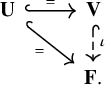
Let . Then, $(u_1, u_2) <_{\mathbf {F}} (u_1, u_5) <_{\mathbf {F}} (u_3, u_4)$ . Thus, $E(\mathbf {F})$ is indeed dense.

Similarly, one can prove the nonexistence of both the smallest and the greatest element of $E(\mathbf {F}) \setminus \{\bot _{\mathbf {F}}\}$ .

Proposition 3.5. Every metric space that induces $\leqslant _{\mathbf {F}}$ is dull (and consequently bounded and uniformly discrete).

Proof. Let $(F, d)$ be some metric space which induces $\mathbf {F}$ . Further, let $\varphi \colon \operatorname {\mathrm {im}} d \to E(\mathbf {F})$ be the naturally induced order-isomorphism. Define . Recall that being dull is equivalent to $\operatorname {\mathrm {im}} d\subseteq [\tau ,2\tau ]\cup \{0\}$ (see the proof of Lemma 1.10).

Fix distinct $x_0, y_0 \in F$ . Recall that $\mathbf {F}$ is universal; thus, for any choice of distinct $x, y \in F$ , there have to exist $u, v, w \in F$ such that

$$\begin{align*}(u, v) \sim_{\mathbf{F}} (x, y), \quad (u, w) \sim_{\mathbf{F}} (v, w) \sim_{\mathbf{F}} (x_0, y_0).\end{align*}$$

Put differently, $ d(u, v) = c$ and $d(u, w) = d(v, w) = c_0$ , where and :

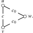
By the triangle inequality, we get $c\leqslant 2c_0$ .

Since $(x,y)$ (and hence c) was arbitrary, we have $\operatorname {\mathrm {im}} d\subseteq [0,2c_0]$ .

By letting $c_0$ converge to $\tau $ , we obtain that $\operatorname {\mathrm {im}} d\subseteq [0,2\tau ]$ . By the definition of $\tau $ , we actually have $\operatorname {\mathrm {im}} d\subseteq \{0\}\cup [\tau ,2\tau ]$ . Hence, $(F, d)$ is dull.

Corollary 3.6. $\mathbf {F}$ is not isomorphic to the echeloned space induced by the (bounded) rational Urysohn space.

Proof. As the (bounded) rational Urysohn space is not dull, it follows by Proposition 3.5 that it cannot induce $\mathbf {F}$ .

However, the echeloned space $\mathbf {F}$ is indeed induced by a dull Urysohn space, as we now explain.

Let $S = \{0\} \cup (1, 2) \cap \mathbb {Q}$ . Consider the S-Urysohn space $\mathbf {U}_S = (U, d_{\mathbf {U}_S})$ , that is, the Fraïssé limit of all finite metric spaces with distances in S (see [26, Theorem 1.4]). Let $\mathbf {M} = (U, \leqslant _{\mathbf {M}})$ be the echeloned space induced on U by $ d_{\mathbf {U}_S}$ .

Proposition 3.7. The echeloned space $\mathbf {M}$ is isomorphic to $\mathbf {F}$ .

Proof. By the uniqueness of Fraïssé limits, it is enough to prove that $\mathbf {M}$ is weakly homogeneous and universal for the class of all finite echeloned spaces.

• Universality Obviously, every finite substructure of $\mathbf {M}$ is a finite echeloned space. Conversely, let $\mathbf {A} = (A, \leqslant _{\mathbf {A}})$ be a finite echeloned space. By Proposition 1.11, we can realize $\leqslant _{\mathbf {A}}$ by a (dull) metric $ d_{\mathbf {A}}$ , whose image is in $\{0\} \cup (1, 2)$ . Since this image is finite, we can moreover assume that $ d_{\mathbf {A}}$ only takes rational values (up to applying an order-automorphism of $\{0\} \cup (1, 2)$ ). We have therefore realized $\mathbf {A}$ as a metric space with distances in S. By the universality of the Urysohn space $\mathbf {U}_S$ , there exists an isometric embedding f of $(A, d_{\mathbf {A}})$ into $(U, d_{\mathbf {U}_S})$ . Such an embedding is also an embedding of the respective induced echeloned spaces; that is, $\mathbf {A}$ indeed embeds into $\mathbf {M}$ .

• Weak homogeneity Let $\mathbf {A} =(A, \leqslant _{\mathbf {A}})$ and $\mathbf {B} = (B, \leqslant _{\mathbf {B}})$ be two finite echeloned spaces such that $\mathbf {A}\le \mathbf {B}$ . Let f be an embedding of $\mathbf {A}$ into $\mathbf {M}$ . We can realize $\mathbf {A}$ as a metric space by using the metric inducing $\leqslant _{\mathbf {M}}$ , that is, by defining

  
  This trivially makes f an isometric embedding of $(A, d_{\mathbf {A}})$ into $(U, d_{\mathbf {U}_S})$ . Now choose any metric $ d_{\mathbf {B}}$ on B, extending $ d_{\mathbf {A}}$ , with image in S and inducing $\leqslant _{\mathbf {B}}$ (such a metric exists since $\mathbf {B}$ is finite and the order of $(1, 2) \cap \mathbb {Q}$ is dense and without minimum nor maximum). By the universality and the weak homogeneity of the Urysohn space $\mathbf {U}_S$ , there exists an isometric embedding g of $\mathbf {B}$ into $\mathbf {U}_S$ such that the diagram
  
  commutes. Obviously, g is also an embedding of the induced echeloned space.

Remark 3.8. Let $\tau _1, \tau _2> 0$ and, for $i = 1, 2$ , let $T_i = T_i^{\prime } \cup \{0\}$ , where $T_i^{\prime }$ is any countably infinite subset of $(\tau _i, 2 \tau _i)$ which is order-dense and without maximum nor minimum. As shown by the above proposition, the $T_i$ -Urysohn space $\mathbf {U}_{T_i}$ induces the echeloned space $\mathbf {F}$ , independently of i. It follows that the isometry groups $\operatorname {\mathrm {Iso}}(\mathbf {U}_{T_1})$ and $\operatorname {\mathrm {Iso}}(\mathbf {U}_{T_2})$ are isomorphic (since they are nothing but the subgroup of $\operatorname {\mathrm {Aut}}(\mathbf {F}, \leqslant _{\mathbf {F}})$ that fixes the echeloning), whereas the spaces $\mathbf {U}_{T_1}$ and $\mathbf {U}_{T_2}$ are not isometric as soon as $T_1 \neq T_2$ .

Echeloned spaces naturally give rise to edge coloured graphs where every edge is coloured by its equivalence class in the corresponding echeloning. We describe now this graph for $\mathbf {F}$ .

Definition 3.9. Let C be a nonempty set. A C-coloured graph $\Gamma $ is an ordered pair $(V, \chi )$ , where V is a set and $\chi \colon [V]^2 \to C$ (here and in the following, we adopt the standard notation that $[V]^2$ refers to the set of $2$ -element subsets of V). V is called the set of vertices and $\chi $ is called the edge-colouring function of $\Gamma $ .

Let us stress that C-coloured graphs are by definition complete graphs.

Definition 3.10. Let $\Gamma _1 = (V_1, \chi _1)$ and $\Gamma _2 = (V_2, \chi _2)$ be two C-coloured graphs, where C is a fixed set of colours. Then a homomorphism from $\Gamma _1$ to $\Gamma _2$ is an injective map $f\colon V_1\to V_2$ such that

$$\begin{align*}\forall \{x, y\} \in [V_1]^2\,:\, \chi_1(\{x, y\}) = \chi_2(\{f(x), f(y)\}).\end{align*}$$

Every C-coloured graph $\Gamma = (V, \chi )$ may be defined equivalently as a relational structure $\mathbf {\Gamma }$ over the signature $\{\varrho _c \mid c \in C\}$ consisting solely of binary relation symbols, where . In particular, a function $h \colon V_1 \to V_2$ is a homomorphism from $\Gamma _1$ to $\Gamma _2$ if and only if it is a homomorphism from $\mathbf {\Gamma }_1$ to $\mathbf {\Gamma }_2$ . This allows us to identify every C-coloured graph $\Gamma $ with its associated relational structure $\mathbf {\Gamma }$ . We shall freely do so without any further notice.

What follows is a characterisation of homogeneous universal countable C-coloured graphs, for countable C, following [28] and [27].

Definition 3.11. Let $\Gamma = (V, \chi )$ be a C-coloured graph, and let k be a positive integer. We say that $\Gamma $ has the $(\ast _k)$ -property if for any $(c_1, c_2, \ldots , c_k) \in C^k$ and any choice of k finite, pairwise disjoint subsets of V, denoted $U_1, U_2, \ldots , U_k$ , there exists a vertex $z \in V$ such that for all $i \in \{1, 2, \dots , k\}$ and all $u \in U_i$ : $\chi (\{z, u\}) = c_i$ . $\Gamma $ is said to have the $(\ast _\infty )$ -property if it has the $(\ast _k)$ -property for all $k \in \mathbb {N}^+$ .

Note that for every $k\in \mathbb {N}^+$ , the $(\ast _{k+1})$ -property implies the $(\ast _k)$ -property.

It is straightforward to check that the class of all finite C-coloured graphs enjoys the amalgamation property, so we obtain the following:

Lemma 3.12. Let C be a countable set of colours. Then the class of all finite C-coloured graphs is a Fraïssé class.

For every countable C, we will denote the universal homogeneous C-coloured graph, that is, the Fraïssé limit of the class of all finite C-coloured graphs, by $\mathcal {T}_C = (V_C, \chi _C)$ .

Proposition 3.13. Let C be countable. Then, a countable C-coloured graph has the $(\ast _\infty )$ -property if and only if it is homogeneous and universal for the class of finite C-coloured graphs.

Proof. ‘ $\Rightarrow $ ’: Let $\Gamma = (V, \chi )$ be a countable C-coloured graph for which the $(\ast _\infty )$ -property holds.

Let us start by showing that $\Gamma $ is universal. We proceed by induction on the size $\ell $ of the C-coloured graph to be embedded. The empty C-coloured graph embeds to $\Gamma $ trivially. Suppose that $\Delta =(W,\eta )$ is a C-coloured graph of size $\ell +1$ . Let $v\in W$ . Let $\Delta '$ be the C-coloured subgraph of $\Delta $ induced by $W\setminus \{v\}$ , and suppose that $\Delta '$ embeds into $\Gamma $ by an embedding $\iota $ . Let $c_1,\dots ,c_k$ be all the (pairwise distinct) colours appearing as a colour of an edge from v in $\Delta $ . For each $i\in \{1,\dots ,k\}$ , let . Note that $\iota (U_1),\dots ,\iota (U_k)$ are pairwise disjoint. By the $(*_{\infty })$ -property (and, therefore, $(*_{k})$ -property), there exists a vertex $z\in V$ such that for all $i\in \{1,\dots ,k\}$ and all $u\in \iota (U_i)\,:\, \chi (\{z,u\})=c_i$ . Hence, the map $\hat {\iota }\colon W\to V$ extending $\iota $ and sending v to z is an embedding of $\Delta $ into $\Gamma $ . This finishes the proof that $\Gamma $ is universal. By iterating the argument above, it becomes clear that $\Gamma $ is also weakly homogeneous in the sense of [12], and hence homogeneous.

‘ $\Leftarrow $ ’: Consider any universal homogenous countable C-coloured graph $\Gamma = (V, \chi )$ . Fix any positive integer k and a tuple $(c_1, \dots , c_k) \in C^k$ . Then choose k finite, pairwise disjoint subsets $U_1, \dots , U_k$ of V. Define a finite C-coloured graph on the set of vertices , where $u \not \in V$ is a new vertex, with the edge-colouring function $\chi _2$ which maps $\{u, v\}$ to $c_i$ for any $v \in U_i$ and $\{v_1, v_2\}$ to $\chi (\{v_1, v_2\})$ for any two distinct $v_1, v_2 \in V_2 \setminus \{u\}$ . Let $\Gamma _1$ be the C-coloured subgraph of $\Gamma $ induced by $\bigcup \limits _{i = 1}^n U_i$ . Clearly, there exist identity embeddings $\iota _1 \colon \Gamma _1 \hookrightarrow \Gamma $ and $\iota _2 \colon \Gamma _1 \hookrightarrow (V_2, \chi _2)$ . Since $\Gamma $ is homogeneous, it is weakly homogeneous in the sense of [12]. Hence, as $\Gamma $ is also universal, there exists an embedding $f \colon (V_2, \chi _2)\to \Gamma $ for which $\iota _1 = f \circ \iota _2$ . As a result, we get that $\chi (\{f(u), f(\iota _2(v))\}) = \chi (\{f(u), \iota _1(v)\})=\chi (\{f(u), v\})=c_i$ for all $i \in \{1, \dots , k\}$ . Thus, the $(\ast _k)$ -property of $\Gamma $ holds.

Observation 3.14. When a C-coloured graph $\Gamma = (V, \chi )$ , for $|C| = 2$ , has the $(\ast _2)$ -property, then the graph $(V, E)$ , with the set of edges E defined for a fixed $c \in C$ as follows:

$$\begin{align*}(u,v) \in E \quad :\Longleftrightarrow \quad \chi(\{u, v\}) = c, \end{align*}$$

is isomorphic to the Rado graph.

We now establish a connection between the Fraïssé limit $\mathbf {F}$ of finite echeloned spaces and the Fraïssé limit $\mathcal {T}_C$ of finite C-coloured graphs:

Proposition 3.15. Fix $k \in \mathbb {N}^+$ and choose pairwise distinct $c_1, \dots , c_k\in E(\mathbf {F})\setminus \{\bot _{\mathbf {F}}\}$ . Define , with $c_\ast \not \in E(\mathbf {F})$ . Then is isomorphic to $\mathcal {T}_C$ , where

$$\begin{align*}\chi \colon [F]^2 \to C,\, \{u, v\} \mapsto \begin{cases} \eta_{\mathbf{F}}(u, v)& \text{if } \eta_{\mathbf{F}}(u, v) \in \{c_1, \dots, c_k\},\\ c_\ast& \text{otherwise}. \end{cases} \end{align*}$$

Proof. By Proposition 3.13, $\Gamma _C $ is isomorphic to $\mathcal {T}_C$ if it has the $(\ast _\infty )$ -property. As $|C| = k + 1$ , it suffices to show that $\Gamma _C$ has the $(\ast _{k+1})$ -property. Consider thus the $(k+1)$ –tuple $(c_1, \dots , c_k, c_\ast )$ . Without loss of generality, assume $c_1 <_{E(\mathbf {F})} c_2 <_{E(\mathbf {F})} \dots <_{E(\mathbf {F})} c_k$ .

Let $U_1, \dots , U_k, U_* \subseteq F$ be finite and pairwise disjoint. Set . Further, let U be a finite superset of $U'$ such that for all $i \in \{1 \dots , k\}$ , there exist $v_1, v_2 \in U$ for which $\chi (\{v_1, v_2\}) = c_i$ . Further, let $w \not \in F$ be a new point, , and let $\mathbf {U}$ be the echeloned subspace of $\mathbf {F}$ induced by U. We define an echelon $\leqslant _{\mathbf {V}}$ on V such that

• ○ $\leqslant _{\mathbf {V}} \cap ~U^2 =\ \leqslant _{\mathbf {U}} (=\ \leqslant _{\mathbf {F}} \cap ~U^2)$ ,

• ○ for all $i\in \{1,\dots ,k\}$ , for any $v_1,v_2 \in V$ such that $\chi (\{v_1,v_2\})=c_i$ , and for all $u\in U_i$ , $(w, u) \sim _{\mathbf {V}} (v_1, v_2)$ ,

• ○ for any $u_1,u_2 \in U_*$ and $(x, y) \in U^2$ , $(x, y) <_{\mathbf {V}} (w, u_1)\sim _{\mathbf {V}} (w,u_2)$ .

By the construction $\mathbf {U}$ is a subspace of $\mathbf {V}$ . Since $\mathbf {F}$ is universal and weakly homogeneous, there exists an embedding $h \colon \mathbf {V} \hookrightarrow \mathbf {F}$ such that the following diagram commutes:

(†)

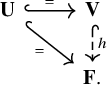
Let . It remains to show that $\chi (\{z, u\}) = c_i$ , whenever $u \in U_i$ for any $i \in \{1, \dots , k\} \cup \{*\}$ .

First, fix $i \in \{1, \dots , k\}$ and $u \in U_i$ . Recall that there exist some $v_1, v_2 \in U$ such that $\chi (\{v_1, v_2\})=c_i$ . In particular, we have $\eta _{\mathbf {F}}(v_1, v_2) = \chi (\{v_1, v_2\}) =c_i$ . By construction, we have $(w,u) \sim _{\mathbf {V}} (v_1, v_2)$ . Thus, $(h(w), h(u)) \sim _{\mathbf {F}} (h(v_1), h(v_2))$ . By the commutativity of diagram (†), we obtain that $(z,u)\sim _{\mathbf {F}} (v_1,v_2)$ . As a result, $\chi (\{z, u\}) = \eta _{\mathbf {F}}(z, u) = \eta _{\mathbf {F}}(v_1, v_2) = c_i$ .

It remains to show that $\chi (\{z, u\}) = c_\ast $ for all $u \in U_*$ . Let $u \in U_*$ be arbitrary. Then by definition of $\leqslant _{\mathbf {V}}$ , we know that for $i \in \{1, \dots , k\}$ and any $(v_1, v_2) \in U^2$ with $\chi (\{v_1, v_2\}) = c_i$ , we have $(v_1, v_2) <_{\mathbf {V}} (w, u)$ . We get that $(h(v_1), h(v_2)) <_{\mathbf {F}} (h(w), h(u))$ , and hence, by the commutativity of diagram (†), $(v_1, v_2) <_{\mathbf {F}} (z, u)$ . In particular, $\eta _{\mathbf {F}}(z, u) \not = \eta _{\mathbf {F}}(v_1, v_2) = c_i$ for any $i \in \{1, \dots , k\}$ . Consequently, $\chi (\{z, u\}) = c_\ast $ .

Corollary 3.16. For any $c \in E(\mathbf {F}) \setminus \{\bot _{\mathbf {F}}\}$ , the graph $(F, E)$ with the set of edges defined by

$$\begin{align*}\{u, v\} \in E \quad :\Longleftrightarrow \quad \eta_{\mathbf{F}}(u, v) = c\end{align*}$$

is isomorphic to the Rado graph.

Proof. Fix a $c \in E(\mathbf {F}) \setminus \{\bot _{\mathbf {F}}\}$ and pick any $c_\ast \not \in E(\mathbf {F})$ . Define

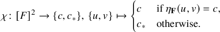$$\begin{align*}\chi \colon [F]^2 \to \{c, c_\ast\},\, \{u, v\} \mapsto \begin{cases} c& \text{if } \eta_{\mathbf{F}}(u, v) = c,\\ c_\ast& \text{otherwise}. \end{cases} \end{align*}$$

By Proposition 3.15, $(F, \chi ) \cong \mathcal {T}_C$ , with $C = \{c, c_\ast \}$ . Consequently, by Observation 3.14, $(F, E)$ is then isomorphic to the Rado graph.

Theorem 3.17. Fix . Then, the C-coloured graph $(F, \chi )$ with

$$\begin{align*}\chi \colon [F]^2 \to C,\quad \{u, v\} \mapsto \eta_{\mathbf{F}}(u, v) \end{align*}$$

is isomorphic to $\mathcal {T}_C$ .

Proof. Fix a positive integer $k \geqslant 2$ . Pick any k colours from C and enumerate them as $\{c_1, c_2, \dots , c_k\}$ . Also, choose any k pairwise disjoint finite sets of points $U_1, U_2, \dots , U_k$ from F. Let $c_{k+1}\in C\setminus \{c_1,\dots , c_k\}$ . Define and a colouring

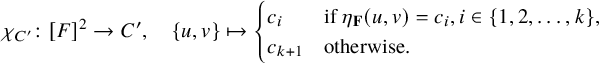$$\begin{align*}\chi_{C'} \colon [F]^2 \to C',\quad \{u,v\} \mapsto \begin{cases} c_i& \text{if } \eta_{\mathbf{F}}(u, v) = c_i, i \in \{1, 2, \dots, k\},\\ c_{k+1}& \text{otherwise}. \end{cases} \end{align*}$$

By Proposition 3.15, $(F, \chi _{C'})$ is isomorphic to $\mathcal {T}_{C'}$ . In particular, it enjoys the $(\ast _{k})$ -property. Therefore, there exists a vertex $z \in F$ such that for any $i \in \{1, 2, \dots , k\}$ , $\chi _{C'}(\{u, z\}) =\chi (\{u,z\})= c_i$ for all $u \in U_i$ . Owing to the arbitrary choice of $U_i$ ’s, we get that $(F, \chi )$ itself has the $(\ast _k)$ -property. Due to the arbitrary choice of k, $(F, \chi )$ has the $(\ast _\infty )$ -property and so by Proposition 3.13, it is indeed isomorphic to $\mathcal {T}_C$ .

From this point on, $\mathcal {T}_{\mathbf {F}}$ will always stand for the C-coloured graph described in Theorem 3.17.

Corollary 3.18. Let $\mathbf {H}$ be a finite echeloned space. Let $\bot _{\mathbf {H}}<c_1<\cdots <c_k$ be an enumeration of $E(\mathbf {H})$ . Then for all $d_1<\cdots <d_k\in E(\mathbf {F}) \setminus \{\bot _{\mathbf {F}}\}$ , there exists an embedding $\iota \colon H\hookrightarrow F$ such that $\hat {\iota }(c_i)=d_i$ for all $i\in \{1,\dots ,k\}$ .

Proof. Let . Let $\Gamma $ be the C-coloured graph $(H,\chi )$ with $\chi (\{u,v\})=d_i$ if $\eta _{\mathbf {H}}(u,v)=c_i$ . By the universality of $\mathcal {T}_{\mathbf {F}}$ established in Theorem 3.17, there exists an embedding $\kappa \colon \Gamma \hookrightarrow \mathcal {T}_{\mathbf {F}}$ of C-coloured graphs. It induces an embedding $\iota \colon \mathbf {H}\hookrightarrow \mathbf {F}$ with $\hat {\iota }(c_i)=d_i$ .

Below, we show that universal homogeneous C-coloured graphs, for countable C, can be constructed probabilistically.

Proposition 3.19. Let C be a countable set of colours, let V be a countably infinite set, and let $\mu \in \ell ^1(C)$ be a probability measure such that $\mu (c)> 0$ for any colour $c \in C$ . Let $\chi : [V]^2 \to C$ be a random colouring that assigns independently the colour c with probability $\mu (c)$ ; that is,

$$\begin{align*}\forall u,v,\,u\neq v\colon P[\chi (\{u,v\})=c]=\mu(c). \end{align*}$$

Then, with probability 1, the graph $(V,\chi )$ is isomorphic to $\mathcal {T}_C$ .

Proof. We show that $(V,\chi )$ has the $(\ast _\infty )$ -property with probability $1$ . Thus, we fix some integer $k \geqslant 2$ .

Let $U_1,\dots ,U_k$ be disjoint finite subsets of V. Let $c_1,\dots ,c_k\in C$ . Take arbitrary $z\in V$ . We compute the probability that z is not eligible for the $(\ast _\infty )$ -property; that is,

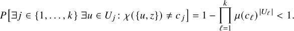$$\begin{align*}P\left[\exists j\in \{1,\dots, k\}\; \exists u\in U_j\colon \chi(\{u,z\})\neq c_j\right] = 1 - \prod_{\ell = 1}^k \mu(c_\ell)^{|U_\ell|} < 1. \end{align*}$$

Since edges are coloured independently, we have

$$\begin{align*}P[\forall z\in V\;\exists j\in \{1,\dots, k\}\; \exists u\in U_j\colon \chi(\{u,z\})\neq c_j]=0. \end{align*}$$

There are only countably many choices for $U_j$ and $c_j$ , so

$$\begin{align*}P[(\ast_\infty)\text{-property fails}]=0. \end{align*}$$

Hence, our observed graph is isomorphic to $\mathcal {T}_C$ (with probability $1$ ).

4 The Ramsey property

Let $\mathcal {K}$ be a class of relational structures. For $\mathbf {A}, \mathbf {B} \in \mathcal {K}$ , denote by $\binom {\mathbf {B}}{\mathbf {A}}$ the set of all substructures of $\mathbf {B}$ isomorphic to $\mathbf {A}$ . Then a class $\mathcal {C}$ is a Ramsey class if for every two structures $\mathbf {A} \in \mathcal {C}$ and $\mathbf {B} \in \mathcal {C}$ and every $k \in \mathbb {N}^+$ , there exists a structure $\mathbf {C} \in \mathcal {C}$ such that the following holds: For every partition of $\binom {\mathbf {C}}{\mathbf {A}}$ into k classes, there is $\tilde {\mathbf {B}} \in \binom {\mathbf {C}}{\mathbf {B}}$ such that $\binom {\tilde {\mathbf {B}}}{\mathbf {A}}$ belongs to a single class of the partition. A countable relational structure $\mathcal {F}$ has the Ramsey property if $\operatorname {Age}(\mathcal {F})$ is a Ramsey class.

Naturally, the question of whether or not the class of finite echeloned spaces is a Ramsey class arises. Homogeneous structures do not necessarily have the Ramsey property. For ordered homogeneous structures, the Kechris-Pestov-Todorčević Theorem gives a necessary and sufficient criterion. It connects the Ramsey property with topological dynamics. Before stating this Theorem, let us recall some key notions:

Let G be a topological group – that is, a group equipped with a topology with respect to which both, multiplication and inverse map are continuous functions. A G-flow is a continuous action $G \times X \to X$ , where X is a nonempty compact Hausdorff space. We say that G is extremely amenable if every G-flow has a fixed point. Recall also that a structure $\mathbf {A}$ whose signature contains a distinguished binary relation symbol $\preceq $ is said to be ordered if $\preceq _{\mathbf {A}}$ is a linear order.

Theorem 4.1 (Kechris, Pestov, Todorčević [15])

Let $\mathcal {K}$ be a Fraïssé class of ordered structures and let $\mathbf {A}$ be its Fraïssé limit. Then $\operatorname {\mathrm {Aut}}(\mathbf {A})$ is extremely amenable if and only if $\mathcal {K}$ is Ramsey.

Now, we begin our exposition by observing that the key feature of a Fraïssé class – namely, the amalgamation property – holds for our class of interest.

Proposition 4.2. The classes of ordered finite echeloned spaces and of ordered finite C-coloured graphs (for countable C) are Fraïssé classes.

Proof. The classes of finite echeloned spaces, finite C-coloured graphs and finite linear orders are all Fraïssé classes with the strong amalgamation property (for the case of finite echeloned spaces, see Remark 3.2). This immediately implies the result (see [5, Section 3.9, p. 59]).

The Fraïssé limit of the class of finite ordered echeloned spaces is actually obtained from $\mathbf {F}$ by the addition of an appropriate linear order $\preceq _{\mathbf {F}}$ isomorphic to the natural order on $\mathbb {Q}$ . We will denote this Fraïssé limit by $(\mathbf {F}, \preceq _{\mathbf {F}})$ .

Lemma 4.3. Let . Then $(\mathcal {T}_{\mathbf {F}},\preceq _{\mathbf {F}})$ is a universal homogeneous ordered C-coloured graph.

Proof. Let $(\mathbf {H},\preceq _{\mathbf {H}})$ be the ordered echeloned space whose echelon $\leqslant _{\mathbf {H}}$ is defined by

$$\begin{align*}(x,y)\leqslant_{\mathbf{H}} (u,v) \quad :\Longleftrightarrow \quad \chi_{\mathbf{H}}(\{x,y\})\leqslant \chi_{\mathbf{H}}(\{u,v\}), \end{align*}$$

from the edge colouring $\chi _{\mathbf {H}}\colon [H]^2\to C$ of a countable homogeneous ordered C-coloured graph $(H,\chi _{\mathbf {H}},\preceq _{\mathbf {H}})$ . We aim to show that $(\mathbf {H}, \preceq _{\mathbf {H}})$ is a universal homogeneous ordered echeloned space. To this end, it suffices to show that $(\mathbf {H},\preceq _{\mathbf {H}})$ is universal and weakly homogeneous. Let $(\mathbf {A},\preceq _{\mathbf {A}})$ be a finite ordered echeloned subspace of $(\mathbf {H},\preceq _{\mathbf {H}})$ , let $(\mathbf {B},\preceq _{\mathbf {B}})$ be a finite ordered echeloned space, and let $\iota \colon (\mathbf {A},\preceq _{\mathbf {A}})\hookrightarrow (\mathbf {B},\preceq _{\mathbf {B}})$ be an embedding. Note that $\kappa \colon E(\mathbf {A})\setminus \{\bot _{\mathbf {A}}\}\to C,\, [(x,y)]_{\sim _{\mathbf {A}}}\mapsto \chi _{\mathbf {H}}(\{x,y\})$ is an order embedding. The same holds for $\hat \iota \colon E(\mathbf {A})\hookrightarrow E(\mathbf {B})$ . Let $\tilde \iota \colon E(\mathbf {A})\setminus \{\bot _{\mathbf {A}}\}\hookrightarrow E(\mathbf {B})\setminus \{\bot _{\mathbf {B}}\}$ be the appropriate restriction of $\hat \iota $ . Recall that C is isomorphic to $\mathbb {Q}$ . In other words, it is a universal homogeneous chain. Thus, there exists an order embedding $\tilde \kappa \colon E(\mathbf {B})\setminus \{\bot _{\mathbf {B}}\}\hookrightarrow C$ that makes the following diagram commutative:

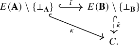
Next we define

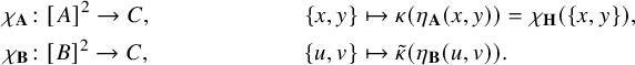$$ \begin{align*} \chi_{\mathbf{A}}&\colon [A]^2\to C, & \{x,y\} &\mapsto \kappa(\eta_{\mathbf{A}}(x,y)) = \chi_{\mathbf{H}}(\{x,y\}),\\ \chi_{\mathbf{B}}&\colon [B]^2\to C, & \{u,v\}&\mapsto \tilde\kappa(\eta_{\mathbf{B}}(u,v)). \end{align*} $$

Then $\iota \colon (A,\chi _{\mathbf {A}},\preceq _{\mathbf {A}})\to (B,\chi _{\mathbf {B}},\preceq _{\mathbf {B}})$ is an embedding of ordered C-coloured graphs. Indeed, $\iota $ preserves $\preceq $ , and

$$ \begin{align*} \forall \{x,y\}\in[A]^2\,:\, \chi_{\mathbf{B}}(\{\iota(x),\iota(y)\}) & = \tilde\kappa (\eta_{\mathbf{B}}(\iota(x),\iota(y)))\\ &= \tilde\kappa(\tilde\iota(\eta_{\mathbf{A}}(x,y))) = \kappa(\eta_{\mathbf{A}}(x,y)) = \chi_{\mathbf{A}}(\{x,y\}). \end{align*} $$

Next, note that $(A,\chi _{\mathbf {A}},\preceq _{\mathbf {A}})$ is an ordered C-coloured subgraph of $(H,\chi _{\mathbf {H}},\preceq _{\mathbf {H}})$ . Indeed, $A\subseteq H$ , ${\preceq _{\mathbf {A}}}\subseteq {\preceq _{\mathbf {H}}}$ , and

$$\begin{align*}\forall\{x,y\}\in[A]^2\,:\, \chi_{\mathbf{A}}(\{x,y\}) = \kappa(\eta_{\mathbf{H}}(x,y)) = \chi_{\mathbf{H}}(\{x,y\}), \end{align*}$$

by the definition of $\kappa $ .

Since $(H,\chi _{\mathbf {H}},\preceq _{\mathbf {H}})$ is universal and weakly homogeneous, there exists $\varepsilon \colon (B,\chi _{\mathbf {B}},\preceq _{\mathbf {B}})\hookrightarrow (H,\chi _{\mathbf {H}},\preceq _{\mathbf {H}})$ , such that the following diagram commutes:

(4.1)

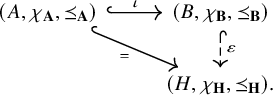
We claim that $\varepsilon \colon (\mathbf {B},\preceq _{\mathbf {B}})\to (\mathbf {H},\preceq _{\mathbf {H}})$ is an embedding. Clearly, $\varepsilon \colon (B,\preceq _{\mathbf {B}})\hookrightarrow (H,\preceq _{\mathbf {H}})$ is an order embedding. So let $(x,y)\leqslant _{\mathbf {B}}(u,v)$ . If $x=y$ , then $\varepsilon (x)=\varepsilon (y)$ , and thus, $(\varepsilon (x),\varepsilon (y))\leqslant _{\mathbf {H}}(\varepsilon (u),\varepsilon (v))$ . If, however, $x\neq y$ , then we compute

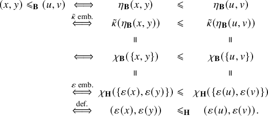
From (4.1), we obtain that

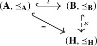
commutes. This shows that $(\mathbf {H},\preceq _{\mathbf {H}})$ is universal and weakly homogeneous.

By the uniqueness of Fraïssé limits, there exists an isomorphism $\varphi \colon (\mathbf {F},\preceq _{\mathbf {F}})\to (\mathbf {H},\preceq _{\mathbf {H}})$ . Since

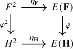
commutes, by the definition of $\chi _{\mathbf {F}}$ and $\chi _{\mathbf {H}}$ , also the following diagram commutes:

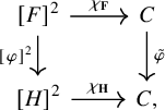
where $[\varphi ]^2\colon \{x,y\}\mapsto \{\varphi (x),\varphi (y)\}$ , and where $\tilde \varphi $ is the appropriate restriction of $\hat \varphi $ to C.

However, this means that $(\mathcal {T}_{\mathbf {F}},\preceq _{\mathbf {F}})$ and $(H,\chi _{\mathbf {H}},\preceq _{\mathbf {H}})$ are practically equal, up to names of vertices and names of colours. In other words, $(\mathcal {T}_{\mathbf {F}},\preceq _{\mathbf {F}})$ is a universal homogeneous C-coloured graph, too.

Lemma 4.4. $\operatorname {\mathrm {Aut}}(\mathcal {T}_{\mathbf {F}}, \preceq _{\mathbf {F}})$ is extremely amenable.

Proof. By Theorem 4.1, it suffices to prove that the class of finite ordered C-coloured graphs is Ramsey. In order to show this, we consider the class of all finite ordered C-coloured graphs, where . Let $c\in C$ .

Note that there exists a canonical bijection $\Phi $ between the class of all ordered C-coloured graphs and all ordered $C\setminus \{c\}$ -edge-coloured (simple) graphs such that, for all ordered C-coloured graphs $\mathbf {A}$ and $\mathbf {B}$ ,

1. (i) $\Phi (\mathbf {A})$ has the same vertex set as $\mathbf {A}$ , and

2. (ii) the set of embeddings from $\mathbf {A}$ to $\mathbf {B}$ coincides with the set of embeddings from $\Phi (\mathbf {A})$ to $\Phi (\mathbf {B})$ .

In particular, $\Phi (\mathbf {A})$ is obtained from $\mathbf {A}$ through replacing all c-coloured edges by non-edges.

Clearly, the class of finite $C\setminus \{c\}$ -edge-coloured graphs has the free amalgamation property (in the sense of [18, page 1602]); thus, the class of finite ordered $C\setminus \{c\}$ -edge-coloured graphs is a Ramsey class, by a result of Hubička and Nešetril [14, Corollary 4.2, p. 51].

Thanks to the properties of $\Phi $ ( $\Phi $ is an isomorphism between the category of C-coloured graphs with embeddings and the category of $C\setminus \{c\}$ -edge-coloured graphs with embeddings), the class of finite ordered C-coloured graphs is Ramsey, too. So $\operatorname {\mathrm {Aut}} (\mathcal {T}_{\mathbf {F}},\preceq _{\mathbf {F}})$ is extremely amenable due to Theorem 4.1.

For the notation used in the following lemma, see Corollary 1.4.

Lemma 4.5. Let $\beta $ be a local isomorphism of $E(\mathbf {F})\setminus \{\bot _{\mathbf {F}}\}$ , with . Then, there exists an automorphism $\alpha $ of $(\mathbf {F}, \preceq _{\mathbf {F}})$ such that $\hat {\alpha }\mathord {\upharpoonright }_{T} = \beta $ .

Proof. Recall from Lemma 4.3 that $(\mathcal {T}_{\mathbf {F}},\preceq _{\mathbf {F}}) = (F,\chi ,\preceq _{\mathbf {F}})$ is a universal homogeneous ordered C-coloured graph, where . Denote the elements of $\operatorname {\mathrm {dom}}\beta $ by $c_1,\dots ,c_k$ and let for each $i\in \{1,\dots ,k\}$ . Let $c_\ast \in C$ be strictly greater than any element of $\{c_1,\dots ,c_k,c_{k+1},\dots ,c_{2k}\}$ . Consider the ordered C-coloured graphs $(\Delta ,\preceq _\Delta )=(D,\chi _{\Delta },\preceq _\Delta )$ and $(\tilde \Delta ,\preceq _{\tilde \Delta })=(\tilde {D},\chi _{\tilde \Delta },\preceq _{\tilde \Delta })$ given by

• ○ $D=\{v_1,\dots ,v_{k}\}\mathrel {\dot \cup } \{w_1,\dots ,w_{k}\}$ , $v_1\preceq _\Delta \dots \preceq _\Delta v_k\preceq _\Delta w_1\preceq _\Delta \dots \preceq _\Delta w_k$ , and

• ○ $\chi _{\Delta }(\{x,y\})=\begin {cases} c_i & \text {if } \{x,y\}=\{v_i,w_i\} \text { for some } i\in \{1,\dots ,k\},\\ c_\ast & \text {else}. \end {cases}$

• ○ $\tilde {D}=\{\tilde {v}_1,\dots ,\tilde {v}_{k}\}\mathrel {\dot \cup } \{\tilde {w}_1,\dots ,\tilde {w}_{k}\}$ , $\tilde {v}_1\preceq _\Delta \dots \preceq _\Delta \tilde {v}_k\preceq _\Delta \tilde {w}_1\preceq _\Delta \dots \preceq _\Delta \tilde {w}_k$ , and

• ○ $\chi _{\tilde \Delta }(\{x,y\})=\begin {cases} c_{k+i} & \text {if } \{x,y\}=\{\tilde {v}_i,\tilde {w}_i\} \text { for some } i\in \{1,\dots ,k\},\\ c_\ast & \text {else}. \end {cases}$

Since $(\mathcal {T}_{\mathbf {F}},\preceq _{\mathbf {F}})$ is universal, both $(\Delta ,\preceq _\Delta )$ and $(\tilde \Delta ,\preceq _{\tilde \Delta })$ embed into it. Without loss of generality, we may assume that $(\Delta ,\preceq _\Delta )$ and $(\tilde \Delta ,\preceq _{\tilde \Delta })$ are substructures of $(\mathcal {T}_{\mathbf {F}},\preceq _{\mathbf {F}})$ . Consider

$$\begin{align*}\varphi\colon D\to F \text{ given by } v_i\mapsto\tilde{v}_i,\, w_i\mapsto\tilde{w}_i,\, i=1,\dots, k. \end{align*}$$

We claim that $\varphi $ is an embedding of the ordered echeloned space into $(\mathbf {F},\preceq _{\mathbf {F}})$ . Clearly, $\varphi $ is an order-embedding from $(D,\preceq _\Delta )$ into $(F,\preceq _{\mathbf {F}})$ . Let $(x,y),(u,v)\in D^2$ . Then

By the homogeneity of $(\mathbf {F},\preceq _{\mathbf {F}})$ , there exists an automorphism $\alpha $ of $(\mathbf {F},\preceq _{\mathbf {F}})$ that makes the following diagram commutative:

From the previous calculations, it is clear that $\hat \alpha \mathord {\upharpoonright }_T=\beta $ .

Prior to stating and proving the main result of this section, we recall a natural family of topological groups. Let X be a set. Then the corresponding full symmetric group $\operatorname {Sym}(X)$ , that is, the group of all self-bijections of X, together with the topology of pointwise convergence associated with the discrete topology on X is a topological group. In turn, if G is a subgroup of $\operatorname {Sym}(X)$ , then G, endowed with the relative topology inherited from $\operatorname {Sym}(X)$ , is a topological group, and the sets of the form

constitute a neighborhood basis at the identity in G. If X is countable, then $\operatorname {Sym}(X)$ , as well as any of its closed topological subgroups, is Polish.

The proof of the following result will make use of Theorem 4.1 along with the persistence of extreme amenability of topological groups under extensions (see [22, Corollary 6.2.10]).

Theorem 4.6. $(\mathbf {F}, \preceq _{\mathbf {F}})$ has the Ramsey property.

Proof. Due to Theorem 4.1, $(\mathbf {F}, \preceq _{\mathbf {F}})$ has the Ramsey property if and only if $\operatorname {\mathrm {Aut}} (\mathbf {F}, \preceq _{\mathbf {F}})$ is extremely amenable.

Let . Let $\mathcal {T}_{\mathbf {F}}=(F,\chi )$ be the C-coloured graph constructed in Proposition 3.17. Recall that $(\mathbf {F},\preceq _{\mathbf {F}})$ is the Fraïssé limit of the class of finite ordered echeloned spaces. Therefore, $\operatorname {\mathrm {Aut}}(\mathcal {T}_{\mathbf {F}}, \preceq _{\mathbf {F}})$ is a subgroup of $\operatorname {\mathrm {Aut}}(\mathbf {F}, \preceq _{\mathbf {F}})$ – namely, the one of automorphisms that setwise preserve each equivalence class of $\sim _{\mathbf {F}}$ . Let $\pi \colon \operatorname {\mathrm {Aut}}(\mathbf {F}, \preceq _{\mathbf {F}}) \to \operatorname {\mathrm {Aut}}(E(\mathbf {F})) ,\, \alpha \mapsto \hat {\alpha }$ . Clearly, $\ker (\pi ) = \operatorname {\mathrm {Aut}}(\mathcal {T}_{\mathbf {F}}, \preceq _{\mathbf {F}})$ , which is extremely amenable by Lemma 4.4.

Claim 1. ${\pi }$ is continuous.

Proof of the claim

It suffices to note that, for every $c \in E(\mathbf {F})$ , we have $\pi [V_{\operatorname {\mathrm {Aut}}(\mathbf {F}, \preceq _{\mathbf {F}})}(\{x,y\})] \subseteq V_{\operatorname {\mathrm {Aut}}(E(\mathbf {F}))}(\{c\})$ , where $x,y\in F$ such that $\eta _{\mathbf {F}}(x,y)=c$ .

Claim 2. ${\pi }$ is open onto its image.

Proof of the claim

As $\pi $ is a homomorphism, it is enough to show that, for every finite subset E of F, there exists a finite subset $\tilde {E}$ of $E(\mathbf {F})$ such that

$$\begin{align*}\pi[\operatorname{\mathrm{Aut}}(\mathbf{F}, \preceq_{\mathbf{F}})] \cap V_{\operatorname{\mathrm{Aut}}(E(\mathbf{F}))}(\tilde{E}) \subseteq \pi[V_{\operatorname{\mathrm{Aut}}(\mathbf{F}, \preceq_{\mathbf{F}})}(E)].\end{align*}$$

Let E be a finite subset of F. Define . Let $\gamma \in \pi [\operatorname {\mathrm {Aut}}(\mathbf {F}, \preceq _{\mathbf {F}})] \cap V_{\operatorname {\mathrm {Aut}}(E(\mathbf {F}))}(\tilde {E})$ . There then exists some $\alpha _{0} \in \operatorname {\mathrm {Aut}}(\mathbf {F}, \preceq _{\mathbf {F}})$ with $\pi (\alpha _{0}) = \gamma $ . From $\pi (\alpha _{0}) = \gamma \in V_{\operatorname {\mathrm {Aut}}(E(\mathbf {F}))}(\tilde {E})$ , we infer that $E \to \alpha _{0}[E], \, x \mapsto \alpha _{0}(x)$ is a local isomorphism in $(\mathcal {T}_{\mathbf {F}},\preceq _{\mathbf {F}})$ . Since $(\mathcal {T}_{\mathbf {F}},\preceq _{\mathbf {F}})$ is homogeneous by Lemma 4.3, there exists $\alpha _{1} \in \operatorname {\mathrm {Aut}}(\mathcal {T}_{\mathbf {F}},\preceq _{\mathbf {F}})$ such that $\alpha _{1}\mathord {\upharpoonright }_{E} = \alpha _{0}\mathord {\upharpoonright }_{E}$ . We see that . Moreover, as $\alpha _{1} \in \operatorname {\mathrm {Aut}}(\mathcal {T}_{\mathbf {F}},\preceq _{\mathbf {F}})$ , one has $\pi (\alpha _{1}) = \mathrm {id}_{E(\mathbf {F})}$ , so that $\pi (\beta ) = \pi (\alpha _{1})^{-1}\pi (\alpha _{0}) = \pi (\alpha _{0}) = \gamma $ . Hence, $\gamma = \pi (\beta ) \in \pi [V_{\operatorname {\mathrm {Aut}}(\mathbf {F}, \preceq _{\mathbf {F}})}(E)]$ , as desired.

Claim 3. $\pi $ is surjective.

Proof of the claim

We first observe that $\pi [\operatorname {\mathrm {Aut}}(\mathbf {F}, \preceq _{\mathbf {F}})]$ is dense in $\operatorname {\mathrm {Aut}}(E(\mathbf {F}))$ with respect to the topology of pointwise convergence. Indeed, for any $\beta \in \operatorname {\mathrm {Aut}}(E(\mathbf {F}))$ and any finite subset $E_0$ of $E(\mathbf {F})$ , there exists an $\alpha \in \operatorname {\mathrm {Aut}}(\mathbf {F}, \preceq _{\mathbf {F}})$ such that $\pi (\alpha )\mathord {\upharpoonright }_{E_0} = \hat {\alpha } \mathord {\upharpoonright }_{E_0} = \beta \mathord {\upharpoonright }_{E_0}$ , thanks to Lemma 4.5.

Now, by Claims 1 and 2, the topological subgroup $\pi [\operatorname {\mathrm {Aut}}(\mathbf {F}, \preceq _{\mathbf {F}})]$ of $\operatorname {\mathrm {Aut}}(E(\mathbf {F}))$ is actually isomorphic to the quotient of the Polish group $\operatorname {\mathrm {Aut}}(\mathbf {F}, \preceq _{\mathbf {F}})$ by the closed normal subgroup $\ker (\pi )$ . It is therefore itself a Polish group (see, for example, [1, Proposition 1.2.3]) and thus closed in $\operatorname {\mathrm {Aut}}(E(\mathbf {F}))$ (see, for example, [1, Proposition 1.2.1]). Hence, it is equal to $\operatorname {\mathrm {Aut}}(E(\mathbf {F}))$ ; that is, $\pi $ is surjective.

(Note that the previous argument does not actually rely on the separability assumption behind the definition of a Polish space. Indeed, the quotient of a metrizable group, complete for its upper uniform structure, is again complete for its upper uniform structure [3, Corollary 2, p. 27] (see also [4, Theorem 2]) and therefore closed in any group in which it topologically embeds [25, 3.24].)

It follows by these three claims that the group $\operatorname {\mathrm {Aut}}(\mathbf {F}, \preceq _{\mathbf {F}})$ has an extremely amenable closed normal subgroup $\ker (\pi ) = \operatorname {\mathrm {Aut}}(\mathcal {T}_{\mathbf {F}}, \preceq _{\mathbf {F}})$ whose corresponding quotient ${\operatorname {\mathrm {Aut}}(\mathbf {F}, \preceq _{\mathbf {F}})}/{\ker \pi }$ , being isomorphic to $\operatorname {\mathrm {Aut}}(\mathbb {Q}, <)$ by Lemma 3.4, is also extremely amenable [21]. Hence, $\operatorname {\mathrm {Aut}}(\mathbf {F}, \preceq _{\mathbf {F}})$ itself is extremely amenable (see, for example, [22, Corollary 6.2.10]) and therefore $(\mathbf {F}, \preceq _{\mathbf {F}})$ has the Ramsey property by Theorem 4.1.

5 Universality of $\operatorname {\mathrm {Aut}}(\mathbf {F})$

The goal of this section is to prove the following universality property for the automorphism group of the countable universal homogeneous echeloned space $\mathbf {F}$ :

Theorem 5.1. The full symmetric group $\operatorname {Sym}(\mathbb {N})$ topologically embeds into $\operatorname {\mathrm {Aut}}(\mathbf {F})$ (with respect to the pointwise convergence topology).

For a proof of this claim, we are going to employ the theory of Katětov functors in the sense of [17]. If we succeed to equip the class of finite echeloned spaces with a Katětov functor, then from [17, Corollary 3.9, Corollary 3.12], it follows that the automorphism group of every countable echeloned space topologically embeds into $\operatorname {\mathrm {Aut}}(\mathbf {F})$ (with respect to the topology of pointwise convergence). Adding to this the observation that the unique echeloned space on $\mathbb {N}$ with two-element echeloning has automorphism group $\operatorname {Sym}(\mathbb {N})$ , the claim of Theorem 5.1 follows readily.

Note that Theorem 5.1 could be stated stronger. When looking into the details of the Katětov construction, it becomes apparent that actually the natural action of $\operatorname {Sym}(\mathbb {N})$ is, up to action isomorphism, a subaction of the natural action of $\operatorname {\mathrm {Aut}}(\mathbf {F})$ on F (cf. [17, Theorems 2.2, 3.3]).

The rest of this section is devoted to the proof that finite echeloned spaces admit a Katětov functor.

Definition 5.2. Let $\mathcal {C}$ be an age, that is,

• ○ $\mathcal {C}$ is a class of finitely generated structures of the same type,

• ○ $\mathcal {C}$ is isomorphism-closed,

• ○ $\mathcal {C}$ is closed under taking substructures (it has the hereditary property),

• ○ $\mathcal {C}$ has the joint embedding property,

• ○ $\mathcal {C}$ splits into countably many isomorphism classes.

Let $\mathscr {C}$ be a category whose object class consists of all those countably generated structures $\mathbf {X}$ with the property that all finitely generated substructures of $\mathbf {X}$ are in $\mathcal {C}$ , and whose morphism class contains all embeddings. Let $\mathscr {A}$ be the full subcategory of $\mathscr {C}$ induced by $\mathcal {C}$ .

A functor $K\colon \mathscr {A}\to \mathscr {C}$ is called a Katětov functor if

• ○ K preserves embeddings,

• ○ there exists a natural embedding $\lambda \colon \operatorname {Id}\hookrightarrow K$ such that for all $\mathbf {A}\in \mathcal {C}$ and for all one-point extensions $\mathbf {B}$ of $\mathbf {A}$ in $\mathcal {C}$ , there exists an embedding $g\colon \mathbf {B}\hookrightarrow K(\mathbf {A})$ such that the following diagram commutes:

  

Our particular setting is the following:

• ○ $\mathcal {C}$ is the class of all finite echeloned spaces,

• ○ $\mathscr {C}$ is the category of countable echeloned spaces with embeddings,

• ○ $\mathscr {A}$ is the full subcategory of $\mathscr {C}$ induced by $\mathcal {C}$ .

Let $\mathbf {X}=(X,\leqslant _{\mathbf {X}})$ be a finite echeloned space. Suppose that $E(\mathbf {X})=\{\bot _{\mathbf {X}},c_1,\dots ,c_n\}$ , and that

$$\begin{align*}\bot_{\mathbf{X}} <_{E(\mathbf{X})} c_1 <_{E(\mathbf{X})} c_2 <_{E(\mathbf{X})}\dots <_{E(\mathbf{X})} c_n. \end{align*}$$

Let . Let us define a new chain $C_{\mathbf {X}}=(C_{\mathbf {X}},\leqslant _{C_{\mathbf {X}}})$ according to

and

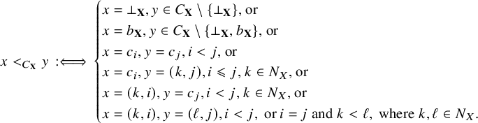$$\begin{align*}x <_{C_{\mathbf{X}}} y \,:\Longleftrightarrow\, \begin{cases} x = \bot_{\mathbf{X}}, y\in C_{\mathbf{X}}\setminus\{\bot_{\mathbf{X}}\}\text{, or}\\ x = b_{\mathbf{X}}, y\in C_{\mathbf{X}}\setminus\{\bot_{\mathbf{X}},b_{\mathbf{X}}\}\text{, or}\\ x = c_i, y= c_j, i<j\text{, or}\\ x = c_i, y = (k,j), i\leqslant j, k\in N_X\text{, or}\\ x = (k,i), y= c_j, i<j, k\in N_X\text{, or}\\ x = (k,i), y = (\ell,j), i<j, \text{ or } i=j \text{ and } k<\ell, \text{ where }k,\ell\in N_X. \end{cases} \end{align*}$$

In other words, $C_{\mathbf {X}}$ can be expressed as an ordinal sum of chains as follows:

$$\begin{align*}\{\bot_{\mathbf{X}}\} \oplus \{b_{\mathbf{X}}\} \oplus (N_X\times\{0\}) \oplus \{c_1\} \oplus (N_X\times\{1\}) \oplus \dots \oplus \{c_n\} \oplus (N_X\times\{n\}). \end{align*}$$

Let now , and define

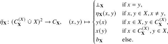$$\begin{align*}\tilde\eta_{\mathbf{X}}\colon(C_{\mathbf{X}}^{(X)}\mathrel{\dot\cup} X)^2\to C_{\mathbf{X}},\quad (x,y)\mapsto\begin{cases} \bot_{\mathbf{X}} & \text{if } x=y,\\ \eta_{\mathbf{X}}(x,y) & \text{if } x, y \in X, x\neq y,\\ y(x) & \text{if } x\in X, y\in C_{\mathbf{X}}^{(X)},\\ x(y) & \text{if } x\in C_{\mathbf{X}}^{(X)},y\in X,\\ b_{\mathbf{X}} & \text{else.} \end{cases} \end{align*}$$

Finally, we define , where

$$\begin{align*}(x,y)\leqslant_{K(\mathbf{X})} (u,v) \quad :\Longleftrightarrow \quad \tilde\eta_{\mathbf{X}}(x,y) \leqslant_{C_{\mathbf{X}}} \tilde\eta_{\mathbf{X}}(u,v). \end{align*}$$

Clearly, $K(\mathbf {X})$ is an echeloned space extending $\mathbf {X}$ . Moreover, $C_{\mathbf {X}}\cong E(K(\mathbf {X}))$ . Denote by $\zeta _{\mathbf {X}}$ the unique isomorphism from $C_{\mathbf {X}}$ to $E(K(\mathbf {X}))$ . Then, in particular, the following diagram commutes:

(5.1)

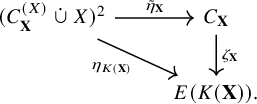
In order to make a functor out of K, we need to define its action on morphisms. In addition to $\mathbf {X}$ let us consider another finite echeloned space $\mathbf {Y}$ . Suppose that $E(\mathbf {Y})= \{\bot _{\mathbf {Y}}, d_1,\dots ,d_m\}$ , where

$$\begin{align*}\bot_{\mathbf{Y}}<_{E(\mathbf{Y})} d_1<_{E(\mathbf{Y})} \dots <_{E(\mathbf{Y})} d_m. \end{align*}$$

Let $\varphi \colon \mathbf {X}\hookrightarrow \mathbf {Y}$ be an embedding; that is, the following diagram commutes:

(5.2)

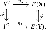
Next, we define

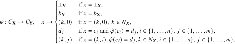$$\begin{align*}\tilde\psi\colon C_{\mathbf{X}}\to C_{\mathbf{Y}},\quad x\mapsto \begin{cases} \bot_{\mathbf{Y}} & \text{if } x=\bot_{\mathbf{X}},\\ b_{\mathbf{Y}} & \text{if } x=b_{\mathbf{X}},\\ (k,0) & \text{if } x=(k,0), \, k\in N_X,\\ d_j & \text{if } x=c_i\text{ and }\hat\varphi(c_i)=d_j, i\in\{1,\dots,n\},\, j\in\{1,\dots,m\},\\ (k,j) & \text{if } x=(k,i), \hat\varphi(c_i)=d_j, k\in N_X, i\in\{1,\dots,n\},\, j\in\{1,\dots,m\}. \end{cases} \end{align*}$$

Clearly, $\tilde \psi $ is an order embedding. Next define

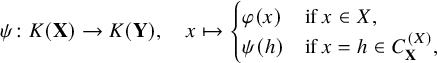$$\begin{align*}\psi\colon K(\mathbf{X})\to K(\mathbf{Y}),\quad x\mapsto\begin{cases} \varphi(x) & \text{if } x\in X,\\ \psi(h) & \text{if } x=h\in C_{\mathbf{X}}^{(X)}, \end{cases} \end{align*}$$

where

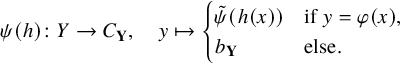(5.3) $$ \begin{align} \psi(h)\colon Y\to C_{\mathbf{Y}},\quad y\mapsto \begin{cases} \tilde\psi(h(x)) & \text{if } y=\varphi(x),\\ b_{\mathbf{Y}} & \text{else.} \end{cases} \end{align} $$

Figure 1 The construction of $\psi $ .

Figure 1 illustrates these definitions. Since $\tilde \psi $ and $\varphi $ are injective, it follows that $\psi $ is injective, too. In order to see that $\psi \colon K(\mathbf {X})\to K(\mathbf {Y})$ is indeed an embedding, according to Corollary 1.4, we need to show that there exists $\hat \psi \colon E(K(\mathbf {X}))\hookrightarrow E(K(\mathbf {Y}))$ such that the following diagram commutes:

(5.4)

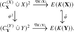
To this end, let us define . Now what remains is to show that the following diagram commutes:

(5.5)

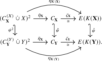
Note that the upper and the lower triangle in (5.5) commute by (5.1). The right-hand rectangle of (5.5) commutes by construction. It remains to check that the left-hand rectangle of (5.5) commutes. For this, we take arbitrary but distinct $x,y\in X$ and $h_1,h_2\in C_{\mathbf {X}}^{(X)}$ , and chase them through this rectangle:

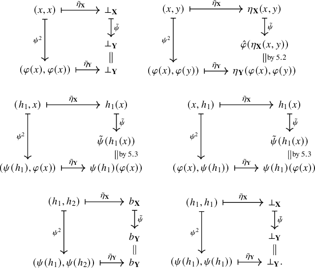
Thus, (5.5) and, in particular (5.4) commute. Consequently, $\psi $ is an embedding of echeloned spaces. Let us define

Now that the action of K on morphisms is defined, we still need to show that K is indeed a functor, that is,

1. (i) $\forall \mathbf {X}\in \mathcal {C}\,:\, K(\mathrm {id}_{\mathbf {X}}) = \mathrm {id}_{K(\mathbf {X})}$ , and

2. (ii) $\forall \varphi _1\colon \mathbf {X}\hookrightarrow \mathbf {Y},\, \varphi _2\colon \mathbf {Y}\hookrightarrow \mathbf {Z}\,:\, K(\varphi _2\circ \varphi _1) = K(\varphi _2)\circ K(\varphi _1)$ .

About (i): For some finite echeloned space $\mathbf {X}$ , consider $K(\mathrm {id}_{\mathbf {X}})\colon C_{\mathbf {X}}^{(X)}\mathrel {\dot \cup } X\to C_{\mathbf {X}}^{(X)}\mathrel {\dot \cup } X$ . Clearly, for each $x\in X$ , we have $K(\mathrm {id}_{\mathbf {X}})(x)= x$ . So let $h\in C_{\mathbf {X}}^{(X)}$ . For simplicity of notation, let us denote $K(\mathrm {id}_{\mathbf {X}})$ by $\psi $ . Then $(K(\mathrm {id}_{\mathbf {X}})(h))(x)= \tilde \psi (h(x))$ , for each $x\in X$ .

• ○ If $h(x)=b_{\mathbf {X}}$ , then $\tilde \psi (h(x)) = \tilde \psi (b_{\mathbf {X}}) = b_{\mathbf {X}}$ ;

• ○ If $h(x)=(k,0)$ , then $\tilde \psi (h(x))= \tilde \psi ((k,0)) = (k,0)$ ;

• ○ If $h(x)=c_i$ , then $\tilde \psi (h(x)) = \tilde \psi (c_i) = \widehat {\mathrm {id}_{\mathbf {X}}}(c_i) = c_i$ ;

• ○ If $h(x) = (k,i)$ , then $\tilde \psi (h(x)) = \tilde \psi ((k,i)) = (k,i)$ , because $\widehat {\mathrm {id}_{\mathbf {X}}}(c_i) = c_i$ ;

Thus, $K(\mathrm {id}_{\mathbf {X}}) = \mathrm {id}_{K(\mathbf {X})}$ .

About (ii): Given

Let us denote , , $\psi _1 = K(\varphi _1)$ , and . Then

Suppose $E(\mathbf {X})=\{\bot _{\mathbf {X}},c_1,\dots ,c_n\}$ , $E(\mathbf {Y}) = \{\bot _{\mathbf {Y}},d_1,\dots ,d_m\}$ , and $E(\mathbf {Z})=\{\bot _{\mathbf {Z}},e_1,\dots ,e_s\}$ , where

$$ \begin{align*} \bot_{\mathbf{X}} <_{E(\mathbf{X})} c_1 <_{E(\mathbf{X})} \dots <_{E(\mathbf{X})} c_n,\quad \bot_{\mathbf{Y}} <_{E(\mathbf{Y})} d_1 &<_{E(\mathbf{Y})} \dots <_{E(\mathbf{Y})} d_m, \\ &\quad \text{and } \bot_{\mathbf{Z}} <_{E(\mathbf{Z})} e_1 <_{E(\mathbf{Z})} \dots <_{E(\mathbf{Z})} e_s. \end{align*} $$

Then for every $x\in X$ , we compute

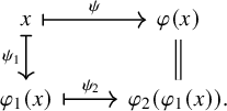
So let $h\in C_{\mathbf {X}}^{(X)}$ . Then

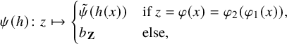$$\begin{align*}\psi(h)\colon z\mapsto \begin{cases} \tilde\psi(h(x)) & \text{if } z=\varphi(x) = \varphi_2(\varphi_1(x)),\\ b_{\mathbf{Z}} & \text{else}, \end{cases} \end{align*}$$

where

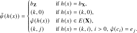$$\begin{align*}\tilde\psi(h(x)) = \begin{cases} b_{\mathbf{Z}} & \text{if } h(x)=b_{\mathbf{X}},\\ (k,0) & \text{if } h(x) = (k,0),\\ \hat\varphi(h(x)) & \text{if } h(x)\in E(\mathbf{X}),\\ (k,j) & \text{if } h(x)=(k,i),\,i>0,\,\hat\varphi(c_i) = e_j. \end{cases} \end{align*}$$

Note that $\hat \varphi = \hat \varphi _2\circ \hat \varphi _1$ (this follows from the uniqueness of $\hat \varphi $ for $\varphi $ ).

However,

$$\begin{align*}(K(\varphi_2)\circ K(\varphi_1))(h) = (\psi_2\circ\psi_1)(h)\in C_{\mathbf{Z}}^{(Z)}, \end{align*}$$

and

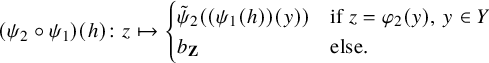$$\begin{align*}(\psi_2\circ\psi_1)(h)\colon z\mapsto \begin{cases} \tilde\psi_2((\psi_1(h))(y)) &\text{if } z=\varphi_2(y),\, y\in Y\\ b_{\mathbf{Z}} & \text{else.} \end{cases} \end{align*}$$

Thus,

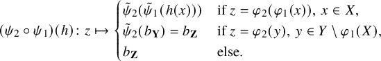$$\begin{align*}(\psi_2\circ\psi_1)(h)\colon z\mapsto\begin{cases} \tilde\psi_2(\tilde\psi_1(h(x))) & \text{if } z=\varphi_2(\varphi_1(x)),\, x\in X,\\ \tilde\psi_2(b_{\mathbf{Y}})=b_{\mathbf{Z}} & \text{if } z=\varphi_2(y),\, y\in Y\setminus\varphi_1(X),\\ b_{\mathbf{Z}} & \text{else.} \end{cases} \end{align*}$$

Figure 2 illustrates the construction of the action of $K(\varphi _2)\circ K(\varphi _1)$ . It remains to check that $\tilde \psi =\tilde \psi _2\circ \tilde \psi _1$ . As usual, we do so by considering possible cases separately. During these computations, assume that for $c_i \in E(\mathbf {X})\setminus \{\bot _{\mathbf {X}}\}$ , we have that $\hat \varphi _1(c_i)=d_\ell $ and $\hat \varphi _2(d_\ell )=e_j$ . Then

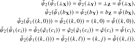$$ \begin{align*} \tilde\psi_2(\tilde\psi_1(\bot_{\mathbf{X}})) = \tilde\psi_2(\bot_{\mathbf{Y}}) = \bot_{\mathbf{Z}} = \tilde\psi(\bot_{\mathbf{X}}),\\ \tilde\psi_2(\tilde\psi_1(b_{\mathbf{X}})) = \tilde\psi_2(b_{\mathbf{Y}}) = b_{\mathbf{Z}} = \tilde\psi(b_{\mathbf{X}}),\\ \tilde\psi_2(\tilde\psi_1((k,0))) = \tilde\psi_2((k,0)) = (k,0) = \tilde\psi((k,0)),\\ \tilde\psi_2(\tilde\psi_1(c_i)) = \tilde\psi_2(\hat\varphi_1(c_i)) = \hat\varphi_2(\hat\varphi_1(c_i)) = \hat\varphi(c_i) = \tilde\psi(c_i),\\ \tilde\psi_2(\tilde\psi_1((k,i))) = \tilde\psi_2((k,\ell)) = (k,j) = \tilde\psi((k,i)). \end{align*} $$

This finishes the proof that K is a functor.

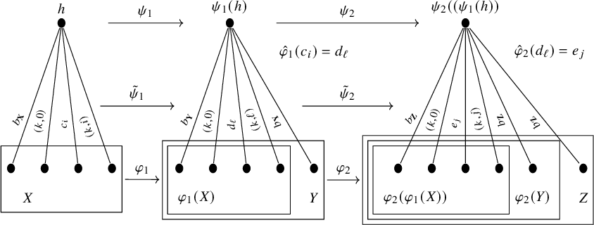
Figure 2 The composition $K(\varphi _2)\circ K(\varphi _1)$ .

Proposition 5.3. $K\colon \mathscr {A}\to \mathscr {C}$ is a Katětov functor.

Proof. Since all the morphisms of $\mathscr {A}$ and $\mathscr {C}$ are embeddings, the condition that K preserves embeddings is trivially fulfilled.

For every finite echeloned space $\mathbf {X}$ , let $\lambda _{\mathbf {X}}\colon \mathbf {X}\hookrightarrow K(\mathbf {X})$ be the identical embedding. It is not hard to check that this defines a natural transformation $\lambda \colon \operatorname {Id}\hookrightarrow K$ .

Let now $\mathbf {X}$ be a finite echeloned space and let $\mathbf {Y}$ be a one-point extension of $\mathbf {X}$ (i.e., $Y=X\mathrel {\dot \cup }\{y\}$ and the identical embedding of X into Y is an embedding of echeloned spaces). Denote the identical embedding of $\mathbf {X}$ into $\mathbf {Y}$ by e. Suppose $E(\mathbf {X})=\{\bot _{\mathbf {X}},c_1,\dots ,c_n\}$ , where

$$\begin{align*}\bot_{\mathbf{X}}<_{E(\mathbf{X})} c_1 <_{E(\mathbf{X})} c_2 <_{E(\mathbf{X})}\dots <_{E(\mathbf{X})} c_n. \end{align*}$$

Then $E(\mathbf {Y})$ is of the shape

$$ \begin{align*} &\bot_{\mathbf{Y}} <_{E(\mathbf{Y})} d_{1,0} <_{E(\mathbf{Y})} \dots d_{i_0,0} <_{E(\mathbf{Y})} \hat{e}(c_1) <_{E(\mathbf{Y})} d_{1,1} <_{E(\mathbf{Y})} \dots \\ &\quad \dots<_{E(\mathbf{Y})} d_{i_1,1} <_{E(\mathbf{Y})} \hat{e}(c_2)<_{E(\mathbf{Y})}\dots <_{E(\mathbf{Y})} \hat{e}(c_n) <_{E(\mathbf{Y})} d_{1,n} <_{E(\mathbf{Y})} \dots <_{E(\mathbf{Y})} d_{i_n,n}, \end{align*} $$

where $i_0+i_1+\dots +i_n\leqslant |X|$ . Define

$$\begin{align*}h\colon X\to C_{\mathbf{X}}\setminus\{\bot_{\mathbf{X}}\},\quad x\mapsto\begin{cases} (k,j) & \text{if } \eta_{\mathbf{Y}}(y,e(x)) = d_{k,j}, \text{ where }j=0,\dots,n,\, k=1,\dots, i_j,\\ c_j & \text{if } \eta_{\mathbf{Y}}(y,e(x)) = \hat{e}(c_j),\text{ where } j=1,\dots,n. \end{cases} \end{align*}$$

Finally, define

$$\begin{align*}g\colon Y\to X\mathrel{\dot\cup} C_{\mathbf{X}}^{(X)},\quad x\mapsto\begin{cases} x & \text{if } x\in X,\\ h & \text{if } x=y. \end{cases} \end{align*}$$

By construction, g is injective. Next, we show that $g\colon \mathbf {Y}\to K(\mathbf {X})$ is an embedding. Let $\gamma \colon E(\mathbf {Y})\to C_{\mathbf {X}}$ be given by

$$\begin{align*}\gamma\colon \hat{e}(c_j)\mapsto c_j,\quad \bot_{\mathbf{Y}}\mapsto\bot_{\mathbf{X}},\quad d_{k,j}\mapsto (k,j)\quad \text{ for all } j\in\{0,\dots,n\},\, k\in \{1,\dots,i_j\}. \end{align*}$$

Clearly, $\gamma $ is an order embedding and the following diagram commutes:

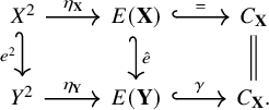
Next, we show that the following diagram commutes, too:

(5.6)

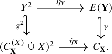
To this end, let $(x,z)\in Y^2$ . We distinguish six cases:

Case 1: Suppose that $x=z\neq y$ . Then

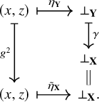
Case 2: Suppose that $x=z=y$ . Then

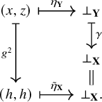
Case 3: Suppose that $x\neq z$ and that $x,z\in X$ . Then $\eta _{\mathbf {X}}(x,z)=c_i$ for some i and

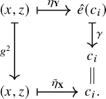
Case 4: Suppose that $x\neq z$ and $x=y$ , and that $\eta _{\mathbf {Y}}(y,e(z))= d_{k,j}$ for some $j\in \{0,\dots ,n\}$ , and $k\in \{1,\dots ,i_j\}$ . Then

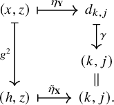
Case 5: Suppose that $x\neq z$ and $x=y$ , and that $\eta _{\mathbf {Y}}(x,e(z))= \hat {e}(c_j)$ for some $j\in \{0,\dots ,n\}$ . Then

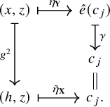
Case 6: If $x\neq z$ and $z=y$ , then we proceed analogously as in cases 4 and 5.

At this point, we may conclude that (5.6) commutes. Combining this with (5.1), we obtain that the following diagram commutes, too:

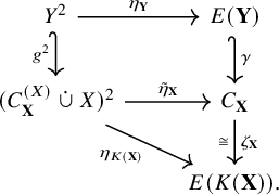
Hence, by Corollary 1.4, g is an embedding with $\hat {g}=\zeta _{\mathbf {X}}\circ \gamma $ .

Finally, by the definition of g, the following diagram commutes:

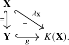
Thus, indeed, K is a Katětov functor.

6 An alternative approach to echeloned spaces

As established in Remark 1.2, an echeloned space may be perceived as a set of points accompanied by a specific $4$ -ary relation. The following definition records yet another, equivalent, approach to these structures.

Definition 6.1. An echeloned map on a set X is a surjective function $f \colon X^2 \twoheadrightarrow (C, \leqslant )$ for which:

1. (i) $(C, \leqslant )$ is a linear order with minimum $\bot _C$ ,

2. (ii) $f^{-1}(\bot _C) = \Delta _X$ , and

3. (iii) $f(x, y) = f(y, x)$ , for all $x, y \in X$ .

We refer to X as the set of points of f.

Remark 6.2. An echeloned map on a set X is finite if X is finite.

Definition 6.3. Let $f \colon X^2 \twoheadrightarrow (C, \leqslant )$ and $g \colon Y^2 \twoheadrightarrow (D, \leqslant )$ be two echeloned maps on X and Y, respectively. We say that a function $\chi \colon X\to Y$ is a homomorphism from f to g, and write $\chi \colon f\to g$ , if there exists an order-preserving map $\bar {\chi } \colon (C, \leqslant ) \rightarrow (D, \leqslant )$ such that the diagram below commutes:

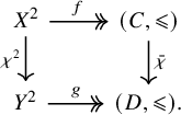
We call $\chi $ an embedding if $\chi $ is injective and $\bar {\chi }$ is an order embedding.

Remark 6.4. If $\bar {\chi }$ in the above definition exists, then it is unique.

Observation 6.5. We describe the connection between echeloned spaces and Definition 6.1 in some detail.

Let $\mathscr {A}$ be the category of echeloned spaces with homomorphisms, and let $\mathscr {B}$ be the category of echeloned maps with homomorphisms. Clearly, if $\mathbf {X} = (X, \leqslant _{\mathbf {X}})$ is an echeloned space, then $\eta _{\mathbf {X}}$ is an echeloned map. Moreover, the homomorphisms between two echeloned spaces are the same as those between their corresponding echeloned maps (see Lemma 1.3). This means that $F \colon \mathscr {A} \to \mathscr {B},\, \mathbf {X} \mapsto \eta _{\mathbf {X}},\, h \mapsto h$ is a well-defined functor.

Now, define a functor $G \colon \mathscr {B} \to \mathscr {A}$ . To every echeloned map $f \colon X^2 \twoheadrightarrow (C, \leqslant )$ , we associate an echeloned space $\mathbf {X}_f = (X, \leqslant _{\mathbf {X}})$ according to the following rule:

$$\begin{align*}(x,y) \leqslant_{\mathbf{X}} (u,v) \quad :\Longleftrightarrow \quad f(x,y) \leqslant f(u, v).\end{align*}$$

Again, by Lemma 1.3, $h \colon f \to g$ is a homomorphism of echeloned maps. Then $h \colon \mathbf {X}_f \to \mathbf {X}_g$ is a homomorphism, too. Hence, the assignment $G\colon \mathscr {B}\to \mathscr {A},\, f \mapsto \mathbf {X}_f,\, h \mapsto h$ is a well-defined functor. Note that $G\circ F = \operatorname {Id}_{\mathscr {A}}$ . Conversely, for each echeloned map $f \colon X^2 \twoheadrightarrow (C, \leqslant )$ , note that the identity function $\mathrm {id}_X$ is an isomorphism from $F(G(f))$ to f. Moreover, $(\varphi _f)_{f\in \operatorname {\mathrm {ob}}(\mathscr {B})}\colon F\circ G\to \operatorname {Id}_{\mathscr {B}}$ with is a natural isomorphism. This shows that $\mathscr {A}$ and $\mathscr {B}$ are equivalent categories. Note that F and G, both, preserve finiteness and embeddings.

All the proofs from the previous sections can be rewritten easily in this alternative approach.