Eisenstein Cohomology for $\mathrm {GL}_N$ and the special values of Rankin–Selberg L-functions over a totally imaginary number field

Abstract

This article presents new rationality results for the ratios of critical values of Rankin–Selberg L-functions of $\mathrm {GL}(n) \times \mathrm {GL}(n')$ over a totally imaginary field $F.$ The proof is based on a cohomological interpretation of Langlands’s contant term theorem via rank-one Eisenstein cohomology for the group $\mathrm {GL}(N)/F,$ where $N = n+n'.$ The internal structure of the totally imaginary base field has a delicate effect on the Galois equivariance properties of the critical values.

Introduction

The principal aim of this article is to prove a rationality result for the ratios of successive critical values of Rankin–Selberg L-functions of $\mathrm {{GL}}(n) \times \mathrm {{GL}}(n')$ over a totally imaginary number field F via a study of rank-one Eisenstein cohomology for the group $\mathrm {{GL}}(N)/F$ , where $N = n+n'.$ This article is a generalization of the methods and results of a previous work with Günter Harder [27] that studied such a situation for a totally real base field. A fundamental tool is the cohomology of local systems on the Borel–Serre compactification of a locally symmetric space for $\mathrm {{GL}}(N)/F$ . The technical heart of the article pertains to analyzing the cohomology of the Borel–Serre boundary, especially for the contribution coming from maximal parabolic subgroups, that leads to an interpretation of the celebrated theorem of Langlands on the constant term of an Eisenstein series in terms of maps in cohomology.

Let F be a totally imaginary number field and $F_0$ its maximal totally real subfield. There is at most one totally imaginary quadratic extension $F_1$ of $F_0$ contained in F, giving us two distinct cases that have a bearing on much that is to follow:

1. 1. CM: when there is indeed such an $F_1$ , then $F_1$ is the maximal CM subfield of F;

2. 2. TR: if not, then put $F_1 = F_0$ ; here, $F_1$ is the maximal totally real subfield of F.

The TR-case imposes the restriction that existence of a critical point for Rankin–Selberg L-functions implies $nn'$ is even. The CM-case, arguably the more interesting of the two, will impose no such restrictions; furthermore, whether F itself is CM ( $F = F_1$ ) or not ( $[F:F_1] \geq 2$ ) has a delicate effect on Galois equivariance properties of the rationality results.

Put $G = G_N = \mathrm {Res}_{F/\mathbb {Q}}(\mathrm {{GL}}(N)/F),$ and $T = T_N$ the restriction of scalars of the diagonal torus in $\mathrm {{GL}}(N).$ Let E stand for a large enough finite Galois extension of $\mathbb {Q}$ in which F can be embedded. The meaning of large enough will be clear from context. Take a dominant integral weight $\lambda \in X^{*}(T \times E),$ and let $\mathcal {M}_{\lambda , E}$ be the algebraic finite-dimensional absolutely-irreducible representation of $G \times E$ with highest weight $\lambda .$ For a level structure $K_f \subset G(\mathbb {A}_f)$ , where $\mathbb {A}_f$ is the ring of finite adeles of $\mathbb {Q},$ let $\widetilde {\mathcal {M}}_{\lambda , E}$ denote the sheaf of E-vector spaces on the locally symmetric space $\mathcal {S}^G_{K_f}$ of G with level $K_f$ (see Section 1.2). A fundamental object of interest is the cohomology group $H^{\bullet }(\mathcal {S}^G_{K_f}, \widetilde {\mathcal {M}}_{\lambda , E})$ . The Borel–Serre compactification $\bar {\mathcal {S}}^G_{K_f} = \mathcal {S}^G_{K_f} \cup \partial \mathcal {S}^G_{K_f}$ gives the long exact sequence

$$ \begin{align*}\ \cdots H^i_c(\mathcal{S}^G_{K_f}, \widetilde{\mathcal{M}}_{\lambda, E}) \stackrel{\mathfrak{i}^{\bullet}}{\longrightarrow} H^i(\bar{\mathcal{S}}^G_{K_f}, \widetilde{\mathcal{M}}_{\lambda,E}) \stackrel{\mathfrak{r}^{\bullet}}{\longrightarrow } H^i(\partial \mathcal{S}^G_{K_f}, \widetilde{\mathcal{M}}_{\lambda,E}) \stackrel{\mathfrak{d}^{\bullet}}{\longrightarrow} H^{i+1}_c( \mathcal{S}^G_{K_f}, \widetilde{\mathcal{M}}_{\lambda, E} ) \cdots \ \end{align*} $$

of modules for the action of a Hecke algebra $\mathcal {H}^G_{K_f}.$ Inner cohomology is defined as ${H^{\bullet }_! = \mathrm {Image}(H^{\bullet }_c \to H^{\bullet }),}$ within which is a subspace $H^{\bullet }_{!!} \subset H^{\bullet }_!$ called strongly-inner cohomology which has the property of capturing cuspidal cohomology at an arithmetic level – that is, for any embedding of fields $\iota : E \to \mathbb {C}$ , one has $H^{\bullet }_{!!}(\mathcal {S}^G_{K_f}, \widetilde {\mathcal {M}}_{\lambda ,E}) \otimes _{E,\iota } \mathbb {C} = H^{\bullet }_{\mathrm {cusp}}(\mathcal {S}^G_{K_f}, \widetilde {\mathcal {M}}_{{}^\iota \lambda , \mathbb {C}}).$ If $\pi _f$ is a simple Hecke module appearing in $H^{\bullet }_{!!}(\mathcal {S}^G_{K_f}, \widetilde {\mathcal {M}}_{\lambda ,E})$ , then ${}^\iota \pi _f$ is the $K_f$ -invariants of the finite part of a cuspidal automorphic representation ${}^\iota \pi $ of $G(\mathbb {A}) = \mathrm {{GL}}_N(\mathbb {A}_F),$ whose archimedean component ${}^\iota \pi _\infty $ has nonzero relative Lie algebra cohomology with respect to $\mathcal {M}_{{}^\iota \lambda , \mathbb {C}}$ ; denote this as $\pi _f \in \mathrm {{Coh}}_{!!}(G,\lambda )$ . Only strongly-pure dominant integral weights will support cuspidal cohomology; the structure of the set $X^+_{00}(T \times E)$ of all such strongly-pure weights has an important bearing on the entire article; see Section 2.3. The cohomology of the Borel–Serre boundary $H^{\bullet }(\partial \mathcal {S}^G_{K_f}, \widetilde {\mathcal {M}}_{\lambda ,E}),$ as a Hecke-module, is built via a spectral sequence from modules that are parabolically induced from the cohomology of Levi subgroups; see Section 2.6. For $N = n+n',$ with positive integers n and $n'$ , similar notations will be adopted for $G_n = \mathrm {Res}_{F/\mathbb {Q}}(\mathrm {{GL}}(n)/F)$ , $T_n$ , $G_{n'}$ , $T_{n'},$ etc. Let $\mu \in X^+_{00}(T_n \times E)$ and $\mu ' \in X^+_{00}(T_{n'} \times E),$ and consider $\sigma _f \in \mathrm {{Coh}}_{!!}(G_n,\mu )$ and $\sigma ^{\prime }_f \in \mathrm {{Coh}}_{!!}(G_{n'},\mu ').$ The contragredient of ${}^{\iota }\sigma ^{\prime }$ is denoted ${}^{\iota }\sigma ^{\prime {\mathrm {v}}}$ . For $\iota : E \to \mathbb {C},$ a point $m \in \tfrac {N}{2} + \mathbb {Z}$ is said to be critical for the completed Rankin–Selberg L-function if the archimedean $\Gamma $ -factors on either side of the functional equation are finite at $s = m.$ The critical set for $L(s, {}^\iota \sigma \times {}^\iota \sigma ^{\prime \mathrm {v}})$ is described in Proposition 3.12. The main result (Theorem 5.16) of this article is the following:

Theorem. Assume that m and $m+1$ are critical for $L(s, {}^\iota \sigma \times {}^\iota \sigma ^{\prime \mathrm {v}}).$

1. (i) If $L(m+1, {}^\iota \sigma \times {}^\iota \sigma ^{\prime \mathrm {v}}) = 0$ for some $\iota $ , then $L(m+1, {}^\iota \sigma \times {}^\iota \sigma ^{\prime \mathrm {v}}) = 0$ for every $\iota .$

2. (ii) Assume F is in the CM-case. Suppose $L(m+1, {}^\iota \sigma \times {}^\iota \sigma ^{\prime \mathrm {v}}) \neq 0$ . Then

   $$ \begin{align*}|\delta_{F/\mathbb{Q}}|^{- \tfrac{n n'}{2}} \cdot \frac{L(m, {}^\iota\sigma \times {}^\iota\sigma^{\prime \mathrm{v}})}{L(m+1, {}^\iota\sigma \times {}^\iota\sigma^{\prime \mathrm{v}})} \ \in \ \iota(E), \end{align*} $$
   where, $\delta _{F/\mathbb {Q}}$ is the discriminant of $F/\mathbb {Q}$ . For any $\gamma \in \mathrm {{Gal}}(\bar {\mathbb {Q}}/\mathbb {Q}),$ we have
   $$ \begin{align*}\kern-10pt & \gamma \left(|\delta_{F/\mathbb{Q}}|^{- \tfrac{n n'}{2}} \cdot \frac{L(m, {}^\iota\sigma \times {}^\iota\sigma^{\prime \mathrm{v}})}{L(m+1, {}^\iota\sigma \times {}^\iota\sigma^{\prime \mathrm{v}})}\right) = \ \varepsilon_{\iota, w}(\gamma) \cdot \varepsilon_{\iota, w'}(\gamma) \cdot |\delta_{F/\mathbb{Q}}|^{- \tfrac{n n'}{2}} \cdot \frac{L(m, {}^{\gamma\circ\iota}\sigma \times {}^{\gamma \circ\iota} \sigma^{\prime \mathrm{v}})}{L(m+1, {}^{\gamma \circ \iota}\sigma \times {}^{\gamma \circ\iota}\sigma^{\prime \mathrm{v}})} \, , \end{align*} $$
   where $ \varepsilon _{\iota , w}(\gamma ), \, \varepsilon _{\iota , w'}(\gamma ) \in \{\pm 1\}$ are certain signatures (see Definition 2.29) whose product is trivial if F is a CM field but can be nontrivial in general.

3. (iii) Assume F is in the TR-case. Then $nn'$ is even. Suppose $L(m+1, {}^\iota \sigma \times {}^\iota \sigma ^{\prime \mathrm {v}}) \neq 0$ . Then

   $$ \begin{align*}\frac{L(m, {}^\iota\sigma \times {}^\iota\sigma^{\prime \mathrm{v}})}{L(m+1, {}^\iota\sigma \times {}^\iota\sigma^{\prime \mathrm{v}})} \ \in \ \iota(E), \end{align*} $$
   and for any $\gamma \in \mathrm {{Gal}}(\bar {\mathbb {Q}}/\mathbb {Q}),$ we have
   $$ \begin{align*}\gamma \left( \frac{L(m, {}^\iota\sigma \times {}^\iota\sigma^{\prime \mathrm{v}})}{L(m+1, {}^\iota\sigma \times {}^\iota\sigma^{\prime \mathrm{v}})}\right) \ = \ \frac{L(m, {}^{\gamma\circ\iota}\sigma \times {}^{\gamma \circ\iota} \sigma^{\prime \mathrm{v}})}{L(m+1, {}^{\gamma \circ \iota}\sigma \times {}^{\gamma \circ\iota}\sigma^{\prime \mathrm{v}})}. \end{align*} $$

For the proof, consider Eisenstein cohomology of $G,$ which, by definition, is the image of $H^{\bullet }(\bar {\mathcal {S}}^G_{K_f}, \widetilde {\mathcal {M}}_{\lambda ,E}) \stackrel {\mathfrak {r}^{\bullet }}{\longrightarrow } H^{\bullet }(\partial \mathcal {S}^G_{K_f}, \widetilde {\mathcal {M}}_{\lambda ,E})$ . We are specifically concerned with the contribution to Eisenstein cohomology from maximal parabolic subgroups; this is often called rank-one Eisenstein cohomology. Let $P = \mathrm {Res}_{F/\mathbb {Q}}(P_{(n,n')})$ , where $P_{(n,n')}$ is the standard maximal parabolic subgroup of $\mathrm {{GL}}_N$ of type $(n,n'),$ and let $U_P$ be the unipotent radical of $P.$ The first technical theorem (Theorem 5.5) stated as the ‘Manin–Drinfeld principle’ says that the algebraically and parabolically induced representation ${{}^{\mathrm {a}}\mathrm { Ind}}_{P(\mathbb {A}_f)}^{G(\mathbb {A}_f)}(\sigma _f \times \sigma ^{\prime }_f)$ together with its partner across a standard intertwining operator splits off as an isotypic component from the cohomology of the boundary as a Hecke module. The next technical result (Theorem 5.6) is to prove that the image of Eisenstein cohomology in this isotypic component is analogous to a line in a two-dimensional plane. If one passes to a transcendental situation using an embedding $\iota : E \to \mathbb {C}$ , then via Langlands’s constant term theorem, the slope of this line is the ratio of L-values $L(m, {}^\iota \sigma \times {}^\iota \sigma ^{\prime \mathrm {v}})/L(m+1, {}^\iota \sigma \times {}^\iota \sigma ^{\prime \mathrm {v}}),$ times the factor $|\delta _{F/\mathbb {Q}}|^{-n n'/2}.$ This latter factor involving the discriminant of the base field arises as the volume of $U_P(\mathbb {Q})\backslash U_P(\mathbb {A})$ needed to normalise the measure so that the constant term map, in cohomology, is the restriction map to the boundary stratum corresponding to P.

There are two subproblems to solve along the way whose proofs are totally different from those of the corresponding statements in [27]. The first is a combinatorial lemma (Lemma 3.16) and the second concerns the map induced in cohomology by the archimedean standard intertwining operator. We now briefly discuss these two subproblems.

The combinatorial lemma (Lemma 3.16) concerns the criticality of L-values that intervene when looking at Eisenstein cohomology. On the one hand, one considers the algebraically induced module ${{}^{\mathrm {a}}\mathrm { Ind}}_{P(\mathbb {A}_f)}^{G(\mathbb {A}_f)}(\sigma _f \times \sigma ^{\prime }_f)$ which appears in boundary cohomology. On the other hand, for the analytic theory of L-functions, one considers the normalized parabolically induced module $I_P^G(s, \sigma \otimes \sigma ')$ as in (5.8), where s is a complex variable. If one specializes the latter at the point of evaluation $s = -N/2$ , then one gets the former module. At this point of evaluation, the L-values that intervene are $L(-N/2, {}^\iota \sigma \times {}^\iota \sigma ^{\prime \mathrm {v}})$ and $L(1-N/2, {}^\iota \sigma \times {}^\iota \sigma ^{\prime \mathrm {v}}).$ Lemma 3.16 characterizes the criticality of these two L-values in terms of a purely combinatorial condition on the weights $\mu $ and $\mu '$ . It also characterizes criticality in terms of the appearance of the induced module considered above in the cohomology of the boundary in an optimal degree; this cohomology degree involves subtleties on the lengths of Kostant representatives in Weyl groups. The ingredient w in the signature $\varepsilon _{\iota , w}(\gamma )$ is a Kostant representative determined by $\mu $ and $\mu '$ via this combinatorial lemma, and $w'$ in $\varepsilon _{\iota , w'}(\gamma )$ is a Kostant representative determined by w via Lemma 5.1. The combinatorial lemma also says that we only need to prove a rationality result for the particular ratio $L(-N/2, {}^\iota \sigma \times {}^\iota \sigma ^{\prime \mathrm {v}})/L(1-N/2, {}^\iota \sigma \times {}^\iota \sigma ^{\prime \mathrm {v}}),$ for a sufficiently general class of weights $\mu $ and $\mu '$ ; see 5.3.2.

Now, we briefly discuss the second subproblem which is taken up in detail in Section 4. Typically, in a cohomological approach to the study of the special values of L-functions, one is confronted with an archimedean subproblem. In our context, it takes the following shape. As a consequence of criticality of the L-values at the point of evaluation, it follows from Casselman–Shahidi [6] that the archimedean induced module $\mathcal {I}_\infty := {{}^{\mathrm {a}}\mathrm { Ind}}_{P(\mathbb {R})}^{G(\mathbb {R})}(\sigma _\infty \times \sigma ^{\prime }_\infty )$ is irreducible. Similarly, one has an irreducible module $\tilde {\mathcal {I}}_\infty := {{}^{\mathrm {a}}\mathrm {Ind}}_{Q(\mathbb {R})}^{G(\mathbb {R})}(\sigma ^{\prime }_\infty (-n) \times \sigma _\infty (n'))$ , where Q is the standard parabolic subgroup associate to P corresponding to the partition $N = n' + n.$ Lastly, one has an archimedean standard intertwining isomorphism $T_\infty $ between these irreducible modules. The second subproblem is to compute the map induced in relative Lie algebra cohomology by the archimedean standard intertwining operator $T_\infty $ . It is a consequence of the combinatorial lemma (Lemma 3.16) that there is a highest weight $\lambda $ on $\mathrm {{GL}}_N/F$ such that both the relative Lie algebra cohomology groups $H^{b_N^F}(\mathfrak {g}_N, {\mathfrak {k}}_N; \mathcal {I}_\infty \otimes \mathcal {M}_\lambda )$ and $H^{b_N^F}(\mathfrak {g}_N, {\mathfrak {k}}_N; \tilde {\mathcal {I}}_\infty \otimes \mathcal {M}_\lambda )$ are one-dimensional for degree $b_N^F = ([F:\mathbb {Q}]/2) \cdot N(N-1)/2$ (see (2.14)) being the optimal degree in cohomology alluded to in the previous paragraph. We then need to compute the isomorphism

$$ \begin{align*}T_\infty^{\bullet} : H^{b_N^{\mathbb{C}}}(\mathfrak{g}_N, {\mathfrak{k}}_N; \mathcal{I}_\infty \otimes \mathcal{M}_\lambda) \to H^{b_N^{\mathbb{C}}}(\mathfrak{g}_N, {\mathfrak{k}}_N; \tilde{\mathcal{I}}_\infty \otimes \mathcal{M}_\lambda) \end{align*} $$

between the two one-dimensional vector spaces. If we, a priori, fix bases for these cohomology groups, then $T_\infty ^{\bullet }$ gives a nonzero scalar. In Proposition 4.32, one proves that this scalar is, up to rational quantities, exactly the ratio of local archimedean L-values. The proof uses a well-known factorization of the standard intertwining operator into rank-one operators; for a simple nontrivial case, see Example 4.30; using such a factorization the computation boils down to a $\mathrm {{GL}}(2)$ -calculation. The reader is referred to Harder [25], where a hope is expressed in general, and verified in the context therein, that the rational number implicit in Proposition 4.32 has a simple shape; this hope should have applications to congruences and the p-adic interpolation of the ratios of L-values considered in this paper.

Previous work on the arithmetic of L-functions over a totally imaginary field especially worth mentioning in the context of this article are as follows. For $n = n' =1$ , the rationality result in $(ii)$ is due to Harder [22, Cor. 4.2.2]. In general, see Blasius [1] and Harder [22] for $\mathrm {{GL}}_1$ , see also Harder–Schappacher [21]; Hida [30] for $\mathrm {{GL}}_2 \times \mathrm {{GL}}_1$ and $\mathrm {{GL}}_2 \times \mathrm {{GL}}_2$ ; Grenie [19] for $\mathrm {{GL}}_n \times \mathrm {{GL}}_n$ ; Harris [29] for standard L-functions for unitary groups which may be construed as a subclass of L-functions for $\mathrm {{GL}}_n \times \mathrm {{GL}}_1$ ; Harder [23] and Mœglin [38] for some general aspects of $\mathrm {{GL}}_n$ –the result contained in $(i)$ is due to Mœglin [38, Sect. 5], although our proof is different from [38]. Furthermore, see the author’s paper [40], Grobner–Harris [14] and Januszewski [33] for $\mathrm {{GL}}_n \times \mathrm {{GL}}_{n-1}$ ; Sachdeva [44] for $\mathrm {{GL}}_3 \times \mathrm {{GL}}_1$ ; and Lin [37], Grobner–Harris–Lin [15], Grobner–Lin [16] and Grobner–Sachdeva [18] for different aspects for $\mathrm {{GL}}_n \times \mathrm {{GL}}_{n'}$ . Among these, the results of [15], [16], [18] and [37] come close in scope to the results of this paper; however, their methods are different and work over a base field that is assumed to be CM, while often needing a polarization assumption on their representations to descend to a unitary group, and in some situations being conditional on expected but unproven hypotheses. In contrast, the method pursued here, which is a generalization of Harder [22] and my work with Harder [26], [27], does not depend on the results of all the other references mentioned above in this paragraph. Furthermore, our results are unconditional in that they do not depend on unproven hypotheses.

There is a celebrated conjecture of Deligne [8, Conj. 2.7] on the critical values of motivic L-functions. A fundamental aspect of the Langlands program is a conjectural dictionary between strongly-inner Hecke modules $\sigma _f$ and pure regular rank n motives $M(\sigma _f)$ over F with coefficients in E (see, for example, [27, Chap. 7]). Granting this dictionary, Deligne’s conjecture applied to $M := \mathrm {Res}_{F/\mathbb {Q}}(M(\sigma _f) \otimes M(\sigma ^{\prime \mathrm {v}}_f))$ conjecturally describes a rationality result for the array $\{L(m, {}^\iota \sigma \times {}^\iota \sigma ^{\prime \mathrm {v}})\}_{\iota : E \to \mathbb {C}}$ of critical values in terms of certain periods $c^\pm (M)$ of M. To see the main theorem of this article from the perspective of motivic L-functions necessitates a relation between $c^+(M)$ and $c^-(M)$ , for which we refer the reader to my recent article with Deligne [9]. The appearance of the signatures $\varepsilon _{\iota , w}(\gamma )$ and $\varepsilon _{\iota , w'}(\gamma )$ was in fact suggested by certain calculations in [9] that also allows us to recast Theorem 5.16 more succinctly as follows. Suppose F is in the CM-case, and suppose $F_1 = F_0(\sqrt {D})$ for a totally negative $D \in F_0$ . Then define $\Delta _{F} = N_{F_0/\mathbb {Q}}(D)^{[F:F_1]/2}.$ Suppose F is in the TR-case. Then define $\Delta _{F} =1.$ Fix ${\mathfrak {i}} = \sqrt {-1}.$ The rationality result can be restated as

$$ \begin{align*}({\mathfrak{i}}^{d_F/2} \Delta_F)^{nn'} \, \frac{L(m, {}^\iota\sigma \times {}^\iota\sigma^{\prime \mathrm{v}})}{L(m+1, {}^\iota\sigma \times {}^\iota\sigma^{\prime \mathrm{v}})} \ \in \iota(E), \end{align*} $$

(see 5.4.2) and the reciprocity law takes the shape that for every $\gamma \in \mathrm {{Gal}}(\bar {\mathbb {Q}}/\mathbb {Q})$ , one has

$$ \begin{align*}\gamma \left( ({\mathfrak{i}}^{d_F/2} \Delta_F)^{nn'} \, \frac{L(m, {}^\iota\sigma \times {}^\iota\sigma^{\prime \mathrm{v}})}{L(m+1, {}^\iota\sigma \times {}^\iota\sigma^{\prime \mathrm{v}})} \right) \ = \ ({\mathfrak{i}}^{d_F/2} \Delta_F)^{nn'} \, \frac{L(m, {}^{\gamma\circ\iota}\sigma \times {}^{\gamma\circ\iota}\sigma^{\prime \mathrm{v}})}{L(m+1, {}^{\gamma\circ\iota}\sigma \times {}^{\gamma\circ\iota}\sigma^{\prime \mathrm{v}})}. \end{align*} $$

In the TR-case, existence of a critical point will necessitate $nn'$ to be even, and so we may ignore the term $({\mathfrak {i}}^{d_F/2} \Delta _F)^{nn'} \in \mathbb {Q}^{\times }$ from the rationality result and the reciprocity law.

To conclude the introduction, let us note that in the literature on special values of L-functions, the shape of the results is often of the form that a critical L-value divided by a ‘period’ is suitably algebraic. To study congruences or p-adic interpolation, the period needs to be normalized up to p-units. One of the virtues of the above theorem on ratios of critical values is that there is no reference to any period; one may construe that the result is intrinsic to the L-function itself. Furthermore, the result opens up new ground to consider the prime factorization of the ratios of L-values; the primes occurring in the denominator (closely related to the denominators of Eisenstein classes; see Harder [24]) should produce some nontrivial elements in a Selmer group as predicted by the Bloch-Kato conjectures. Such considerations will be taken up in a future work. Finally, it is worth amplifying the dictum that whereas the analytic theory of L-functions is not sensitive to the arithmetic nature of the ground field F, the arithmetic of special values of L-functions is definitively sensitive to the inner structure of F. For example, if F is totally real, the Rankin-Selberg integral for $\mathrm {{GL}}(2) \times \mathrm {{GL}}(2)$ does not admit a cohomological interpretation in terms of Poincaré or Serre duality. However, if F is totally imaginary, then it does indeed admit an interpretation in terms of Poincaré duality; see Hida [30]. In a different direction, the period integrals of cusp forms on $\mathrm {{GL}}(2n)$ integrated over $\mathrm {{GL}}(n) \times \mathrm {{GL}}(n)$ that Friedberg–Jacquet [11] studied to get the standard L-function of $\mathrm {{GL}}(2n)$ can be interpreted in cohomology over a totally real field (see my papers with Grobner [17], and with Dimitrov and Januszewski [10]), but over a general number field, this seemed unclear until the recent work of Jiang–Sun–Tian [34]. This dependence on the arithmetic of the base field stems not only from the cohomological vagaries of the representations of $\mathrm {{GL}}_m(\mathbb {R})$ vis-à-vis those of $\mathrm {{GL}}_m(\mathbb {C})$ , but also because the inner structure of the base field informs some of the constructions with algebraic groups over such base fields – this is why one sees the signatures $\varepsilon _{\iota , w}(\gamma )$ and $\varepsilon _{\iota , w'}(\gamma )$ when F is in the CM-case but not when F is in the TR-case; such terms did not appear when the base field is totally real [27] or a CM field [41].

Suggestions to the reader: Any one wishing to read this paper seriously will need my monograph with Harder [27] by their side. I have tried to make this manuscript reasonably self-contained, but any time I felt there was nothing to be gained by repetition, I have referenced [27]. For a finer appreciation, the reader should compare the formal similarities of the results of this manuscript and the results of [27], while noting the very different proofs – especially with the proofs of the combinatorial lemma in Section 3.2, and the calculations involving the archimedean intertwining operator in Section 4. For a first reading, I recommend that the reader skim through Section 1 to get familiar with the notations, and assume the statements of Proposition 3.12, Lemma 3.16, Proposition 4.28 and Proposition 4.32 without worrying too much about their technical proofs. Finally, the reader should note that we are specifically studying the contribution to Eisenstein cohomology only from maximal parabolic subgroups.

1 Preliminaries

1.1 Some basic notation

1.1.1 The base field

Let F stand for a totally imaginary finite extension of $\mathbb {Q}$ of degree $d_F = [F:\mathbb {Q}].$ Let $\Sigma _{F} = \mathrm {{Hom}}(F,\mathbb {C})$ be the set of all complex embeddings, and $\mathrm {S}_\infty $ denote the set of archimedean places of F; denote the cardinality of $\mathrm {S}_\infty $ by ${\mathrm r}$ ; hence, $d_F = 2{\mathrm r}.$ There is a canonical surjection $\Sigma _{F} \to \mathrm {S}_\infty ;$ the fibre over $v \in \mathrm {S}_\infty $ is a pair $\{\eta _v, \bar {\eta }_v\}$ of conjugate embeddings; via such a non-canonical choice of $\eta _v$ , fix the identification $F_v \simeq \mathbb {C}.$ Let $\mathbb {A} = \mathbb {A}_{\mathbb {Q}}$ be the adèle ring of $\mathbb {Q}$ , and $\mathbb {A}_f = \mathbb {A}^\infty $ the ring of finite adèles. Then $\mathbb {A}_F = \mathbb {A} \otimes _{\mathbb {Q}} F$ , and $\mathbb {A}_{F,f} = \mathbb {A}_f \otimes _{\mathbb {Q}} F$ . When F is a CM field (i.e., a totally imaginary quadratic extension of a totally real extension $F^+$ (say) of $\mathbb {Q},$ then $\Sigma _{F^+} = \mathrm {{Hom}}(F^+,\mathbb {C}) = \mathrm {{Hom}}(F^+,\mathbb {R}),$ and the restriction from F to $F^+$ gives a canonical surjection $\Sigma _F \to \Sigma _{F^+}$ ; the fiber over $\eta \in \Sigma _{F^+}$ is a pair of conjugate embeddings that will be denoted as $\{\eta , \bar {\eta }\}$ , with the understanding that the choice of $\eta $ in $\{\eta , \bar {\eta }\}$ though not canonical is nevertheless fixed once and for all. If $\Sigma _F = \{\nu _1, \dots , \nu _{d_F}\}$ , $\{\omega _1,\dots ,\omega _{d_F}\}$ is a $\mathbb {Q}$ -basis of F, and $\theta _F = \det [\sigma _i(\omega _j)]$ , then $\theta _F^2$ is the absolute discriminant $\delta _{F/\mathbb {Q}}$ of F. The square root of the absolute value of the discriminant, $|\delta _{F/\mathbb {Q}}|^{1/2},$ as an element of $\mathbb {R}^{\times }/\mathbb {Q}^{\times },$ is independent of the enumeration and the choice of basis. Let ${\mathfrak {i}}$ denote a fixed choice of $\sqrt {-1}.$ Since F is totally imaginary, ${\mathfrak {i}}^{d_F/2} \cdot \theta _F$ is a real number whose absolute value is $|\delta _{F/\mathbb {Q}}|^{1/2}.$

1.1.2 The groups

For an integer $N \geq 2$ , let $G_{0} = \mathrm {{GL}}_N/F$ , and put $G = \mathrm {Res}_{F/\mathbb {Q}}(G_{0})$ as the $\mathbb {Q}$ -group obtained by the Weil restriction of scalars. To emphasize the dependence on N, $G_0$ will also be denoted $G_{N,0}$ and similar notation will be adopted for other groups to follow. Let $B_0$ be the subgroup of $G_0$ of upper-triangular matrices, $T_0$ the diagonal torus in $B_0$ , and $Z_0$ the center of $G_0$ ; the corresponding $\mathbb {Q}$ -groups via $\mathrm {Res}_{F/\mathbb {Q}}$ will be denoted $B, T$ and Z, respectively. Let S stand for the maximal $\mathbb {Q}$ -split torus of Z; note that $S \simeq \mathbb {G}_m.$ Let n and $n'$ be positive integers such that $n + n' = N,$ and let $P_0$ be the maximal parabolic subgroup of $G_0$ containing $B_0$ of type $(n,n').$ The unipotent radical of $P_0$ is denoted $U_{P_0}$ and Levi quotient of $P_0$ is $M_{P_0} = \mathrm {{GL}}_n \times \mathrm {{GL}}_{n'}.$ Put $P = \mathrm {Res}_{F/\mathbb {Q}}(P_0)$ , and similarly, $U_P$ and $M_P.$ The dimension of $U_P$ is $nn'd_F = 2nn'{\mathrm r}.$

1.2 Sheaves on locally symmetric spaces

This brief section is very similar to the situation over a totally real base field [27]. Most of the concepts in this section apply, possibly with minor modifications, to related groups like $\mathrm {{GL}}_n, \ \mathrm {{GL}}_{n'}, \ M_{P_0},$ etc.

1.2.1 Locally symmetric spaces

Note that $ G(\mathbb {R}) \ = \ G_0(F \otimes _{\mathbb {Q}} \mathbb {R}) \ = \ \prod _{v \in \mathrm {S}_\infty } \mathrm {{GL}}_N(F_v) \ \simeq \ \prod _{v \in \mathrm {S}_\infty } \mathrm {{GL}}_N(\mathbb {C}).$ Similarly, $Z(\mathbb {R}) = Z_0(F \otimes _{\mathbb {Q}} \mathbb {R}) \simeq \prod _{v \in \mathrm {S}_\infty } \mathbb {C}^{\times } 1_N,$ where $1_N$ is the identity $N \times N$ -matrix; $S(\mathbb {R}) = \mathbb {R}^{\times }$ sits diagonally in $Z(\mathbb {R})$ . The maximal compact subgroup of $G(\mathbb {R})$ will be denoted $C_\infty $ ; we have $C_\infty \ = \ \prod _{v \in \mathrm {S}_\infty } \mathrm {{U}}(N),$ where $\mathrm {{U}}(N),$ the usual compact unitary group in N-variables, is a maximal compact group of $\mathrm {{GL}}_N(\mathbb {C})$ . Put $K_\infty = C_\infty S(\mathbb {R})$ and note that $K_\infty = C_\infty S(\mathbb {R})^\circ $ is a connected group, since $-1 \in S(\mathbb {R})$ gets absorbed into $C_\infty .$ Define the symmetric space of G as $\mathcal {S}^G \ := \ G(\mathbb {R})/K_\infty .$ For any open compact subgroup $K_f \subset G(\mathbb {A}_f)$ , define the adèlic symmetric space: $G(\mathbb {A})/K_\infty K_f \ = \ \mathcal {S}^G \times (G(\mathbb {A}_f)/K_f).$ On this space, $G(\mathbb {Q})$ acts properly discontinuously and we get a quotient

(1.1) $$ \begin{align} \pi \, : \, G(\mathbb{R})/K_\infty \times G(\mathbb{A}_f)/K_f \ \longrightarrow \ G(\mathbb{Q}) \backslash \left( G(\mathbb{R})/K_\infty \times G(\mathbb{A}_f)/K_f \right). \end{align} $$

The target space, called the adèlic locally symmetric space of G with level structure $K_f$ , is denoted $\mathcal {S}^G_{K_f} = G(\mathbb {Q}) \backslash G(\mathbb {A}) / K_\infty K_f.$ A typical element in the adèlic group $G(\mathbb {A}) = G(\mathbb {R}) \times G(\mathbb {A}_f)$ will be denoted $\underline g = g_\infty \times { \underline g}_f.$ As in [27, Sect. 2.1.4], one has $\mathcal {S}^G_{K_f} \ \cong \ \coprod _{i=1}^m \ \Gamma _i \backslash G(\mathbb {R}) / K_\infty $ ; if necessary, replacing $K_f$ by a subgroup of finite-index, assume that each $\Gamma _i$ is torsion-free. It is easy to see that $\mathrm {dim}(\mathcal {S}^G_{K_f}) \ = \ \mathrm {dim}(G(\mathbb {R})/K_\infty ) \ = \ \mathrm { dim}(G(\mathbb {R})/C_\infty ) - 1 \ = \ {\mathrm r}N^2 - 1.$

1.2.2 The field of coefficients E

Throughout this paper, let $E/\mathbb {Q}$ be a ‘large enough’ finite Galois extension that takes a copy of $F.$ (The meaning of E being large enough will depend on the context: for example, large enough so that some Hecke summand in inner-cohomology would split over E. To relate cohomology groups with automorphic forms, one could drop finiteness and take $E = \mathbb {C}$ , or anticipating p-adic interpolation of the L-values considered here, E could be a large enough p-adic field.) An embedding $\iota : E \to \mathbb {C}$ gives a bijection $\iota _* : \mathrm {{Hom}}(F,E) \to \mathrm {{Hom}}(F,\mathbb {C})$ given by composition: $\iota _*\tau = \iota \circ \tau .$ If $E = \mathbb {C}$ , then there is a natural notion of complex-conjugation on $\mathrm {{Hom}}(F,\mathbb {C})$ defined by $\bar {\eta }(x) = \overline {\eta (x)}.$ But, on $\mathrm {{Hom}}(F,E)$ , there is no natural notion of complex-conjugation; however, using $\iota : E \to \mathbb {C}$ , we can consider the conjugate $\overline {\tau }^\iota $ of $\tau $ defined as $\iota _*(\overline {\tau }^\iota ) = \overline {\iota _*\tau }.$ If F is a CM field, then let $\{1, c\}$ denote the Galois group of $F/F^+;$ restriction $\tau \mapsto \tau |_{F^+}$ gives a surjective map $\mathrm {{Hom}}(F, E) \twoheadrightarrow \mathrm {{Hom}}(F^+,E);$ for $\tau \in \mathrm {{Hom}}(F, E)$ , define $\tau ^c$ by $\tau ^c(x) = \tau (c(x))$ for all $x \in F$ , then $\{\tau , \tau ^c\}$ is the fiber above $\tau |_{F^+}.$ If $E = \mathbb {C}$ , then $\tau ^c = \bar {\tau }.$

1.2.3 Characters of the torus T

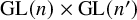
For E as above, let $X^{*}(T \times E) := \mathrm {{Hom}}_{E-\mathrm {alg}}(T \times E, \mathbb {G}_m),$ where $ \mathrm {{Hom}}_{E-\mathrm {alg}}$ is to mean homomorphisms of E-algebraic groups. There is a natural action of $\mathrm {Gal}(E/\mathbb {Q})$ on $X^{*}(T \times E)$ . Since $T = \mathrm {Res}_{F/\mathbb {Q}}(T_0)$ , one has

$$ \begin{align*}X^{*}(T \times E) \ = \ \bigoplus_{\tau : F \to E} X^{*}(T_0 \times_{F,\tau} E) \ = \ \bigoplus_{\tau : F \to E} X^{*}(T_0), \end{align*} $$

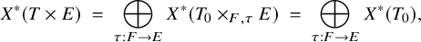
where the last equality is because $T_0$ is split over F. Let $X^{*}_{\mathbb {Q}}(T \times E) = X^{*}(T \times E) \otimes \mathbb {Q}.$ The weights are parametrized as in [27]: $\lambda \in X^{*}_{\mathbb {Q}}(T \times E)$ will be written as $\lambda = (\lambda ^\tau )_{\tau : F \to E}$ with

where is the i-th fundamental weight for $\mathrm {{SL}}_N$ extended to $\mathrm {{GL}}_N$ by making it trivial on the center, and is the determinant character of $\mathrm {{GL}}_N.$ If $r_{\lambda } := (Nd - \sum _{i=1}^{N-1} i (a_i-1))/N,$ then $b_1 = a_1 + a_2 + \dots + a_{N-1} - (N-1) + r_{\lambda }, \ b_2 = a_2 + \dots + a_{N-1} - (N-2) + r_{\lambda }, \dots , b_{N-1} = a_{N-1} - 1 + r_{\lambda }, \ b_N = r_{\lambda },$ and conversely, $a_i - 1 = b_i - b_{i+1}, \ d = (b_1+\dots +b_N)/N.$ A weight is an integral weight if and only if

$$ \begin{align*}\lambda \in X^{*}(T_0) \ \Longleftrightarrow \ b_i \in \mathbb{Z}, \ \forall i \ \Longleftrightarrow \ \left\{\begin{array}{l} a_i \in \mathbb{Z}, \quad 1 \leq i \leq N-1, \\ Nd \in \mathbb{Z}, \\ Nd \equiv \sum_{i=1}^{N-1} i (a_i-1) \quad\pmod{N}. \end{array}\right. \end{align*} $$

A weight $\lambda = (\lambda ^\tau )_{\tau : F \to E} \in X^{*}_{\mathbb {Q}}(T \times E)$ is integral if and only if each $\lambda ^\tau $ is integral. Next, an integral weight $\lambda \in X^{*}(T_0)$ is dominant, for the choice of the Borel subgroup being $B_0$ , if and only if

$$ \begin{align*}b_1 \geq b_2 \geq \dots \geq b_N \ \Longleftrightarrow \ a_i \geq 1 \ \mbox{for } 1 \leq i \leq N-1. \ (\text{There is no condition on } d.) \end{align*} $$

A weight $\lambda = (\lambda ^\tau )_{\tau : F \to E} \in X^{*}_{\mathbb {Q}}(T \times E)$ is dominant-integral if and only if each $\lambda ^\tau $ is dominant-integral. Let $X^+(T \times E)$ stand for the set of all dominant-integral weights.

1.2.4 The sheaf $\widetilde {\mathcal {M}}_{\lambda , E}$

For $\lambda \in X^+(T \times E)$ , put $\mathcal {M}_{\lambda , E} \ = \ \bigotimes _{\tau : F \to E} \mathcal {M}_{\lambda ^\tau },$ where $\mathcal {M}_{\lambda ^\tau }/E$ is the absolutely-irreducible finite-dimensional representation of $G_0 \times _\tau E = \mathrm {{GL}}_n/F \times _\tau E$ with highest weight $\lambda ^\tau .$ Denote this representation as $(\rho _{\lambda ^\tau }, \mathcal {M}_{\lambda ^\tau })$ . The group $G(\mathbb {Q}) = \mathrm {{GL}}_n(F)$ acts on $\mathcal {M}_{\lambda , E}$ diagonally; that is, $a \in G(\mathbb {Q})$ acts on a pure tensor $\otimes _\tau m_\tau $ via $a \cdot (\otimes _\tau m_\tau ) \ = \ \otimes _\tau \rho _{\lambda ^\tau }(\tau (a))(m_\tau ).$ This representation gives a sheaf $\widetilde {\mathcal {M}}_{\lambda , E}$ of E-vector spaces on $\mathcal {S}^G_{K_f}$ : the sections over an open subset $V\subset \mathcal {S}^G_{K_f}$ are the locally constant functions $s: \pi ^{-1}(V) \to \mathcal {M}_{\lambda , E}$ such that $s(a v) = \rho (a) s(v)$ for all $a \in G(\mathbb {Q}),$ where $\pi $ is as in (1.1).

Let us digress for a moment to clarify a certain point that seemingly causes some confusion. In the definition of $\mathcal {S}^G_{K_f},$ one could have divided by $Z(\mathbb {R}) C(\mathbb {R})$ instead of $K_\infty $ ; that is, one can consider $G(\mathbb {Q}) \backslash G(\mathbb {A}) / Z(\mathbb {R}) C(\mathbb {R}) K_f.$ Over this space, the same construction of the sheaf $\widetilde {\mathcal {M}}_{\lambda , E}$ carries through; however, for it to be nonzero, the central character of $\rho _\lambda $ has to have the type of an algebraic Hecke character of F (see [22, 1.1.3]). Let $\lambda = (\lambda ^\tau )_{\tau : F \to E}\in X^+(T \times E)$ , and suppose the condition on the central character means $d^{\iota \circ \tau } + d^{\overline {\iota \circ \tau }}$ is a constant independent every embedding $\iota : E \to \mathbb {C}$ , and every $\tau \in \mathrm {{Hom}}(F,E).$ Define $X^+_{\mathrm {alg}}(T \times E)$ to be the subset of $X^+(T \times E)$ consisting of all dominant-integral weights which satisfy the algebraicity condition that ‘ $d^{\iota \circ \tau } + d^{\overline {\iota \circ \tau }} = \mathrm {constant}$ ’ for all $\tau \in \mathrm {{Hom}}(F,E)$ and for all $\iota : E \hookrightarrow \mathbb {C}$ . To end the digression, for the sheaf $\widetilde {\mathcal {M}}_{\lambda ,E}$ on $\mathcal {S}^G_{K_f}$ , at this moment we do not need to impose this algebraicity condition; however, later on for the sheaf to support interesting cohomology, such as cuspidal cohomology, we will be needing the condition of strong-purity that will imply algebraicity.

If $\lambda \in X^+_{\mathrm {alg}}(T \times E)$ and $K_f$ small enough as in 1.2.1, then every stalk of $\widetilde {\mathcal {M}}_{\lambda , E}$ is isomorphic to the E-vector space $\mathcal {M}_{\lambda ,E},$ in which case the sheaf $\widetilde {\mathcal {M}}_{\lambda ,E}$ is a local system.

2 The cohomology of $\mathrm {{GL}}_N$ over a totally imaginary number field

For $\lambda \in X^+_{\mathrm {alg}}(T \times E)$ , a basic object of study is the sheaf-cohomology group $H^{\bullet }(\mathcal {S}^G_{K_f}, \widetilde {\mathcal {M}}_{\lambda ,E})$ . One of the main tools is a long exact sequence coming from the Borel–Serre compactification. Another tool is the relation of these cohomology groups, by passing to a transcendental situation using an embedding $E \hookrightarrow \mathbb {C}$ , to the theory of automorphic forms on G. The reader should appreciate that Section 2.3 on strongly-pure weights has some novel features that do not show up over a totally real base field or over a CM field.

2.1 Inner cohomology

Let $\bar {\mathcal {S}}^G_{K_f}$ be the Borel–Serre compactification of $\mathcal {S}^G_{K_f}$ , that is, $\bar {\mathcal {S}}^G_{K_f} = \mathcal {S}^G_{K_f} \cup \partial \mathcal {S}^G_{K_f}$ , where the boundary is stratified as $\partial \mathcal {S}^G_{K_f} = \cup _P \partial _P\mathcal {S}^G_{K_f}$ with P running through the $G(\mathbb {Q})$ -conjugacy classes of proper parabolic subgroups defined over $\mathbb {Q}$ . (See Borel–Serre [4].) The sheaf $\widetilde {\mathcal {M}}_{\lambda , E}$ on $\mathcal {S}^G_{K_f}$ naturally extends to a sheaf on $\bar {\mathcal {S}}^G_{K_f}$ which we also denote by $\widetilde {\mathcal {M}}_{\lambda , E}$ . Restriction from $\bar {\mathcal {S}}^G_{K_f}$ to induces an isomorphism in cohomology: $ H^{\bullet }(\bar {\mathcal {S}}^G_{K_f}, \widetilde {\mathcal {M}}_{\lambda , E}) \buildrel \sim \over \longrightarrow H^{\bullet }(\mathcal {S}^G_{K_f}, \widetilde {\mathcal {M}}_{\lambda , E}).$ Consider the Hecke algebra $\mathcal {H}^G_{K_f} = C^\infty _c(G(\mathbb {A}_f)/ \! \!/K_f\kern-1.2pt )$ of all locally constant and compactly supported bi- $K_f$ -invariant $\mathbb {Q}$ -valued functions on $G(\mathbb {A}_f);$ take the Haar measure on $G(\mathbb {A}_f)$ to be the product of local Haar measures, and for every prime p, the local measure is normalized so that $\mathrm {vol}(G(\mathbb {Z}_p)) = 1;$ then $\mathcal {H}^G_{K_f}$ is a $\mathbb {Q}$ -algebra under convolution of functions. The cohomology of the boundary $H^{\bullet }(\partial \mathcal {S}^G_{K_f}, \widetilde {\mathcal {M}}_{\lambda , E})$ and the cohomology with compact supports $H^{\bullet }_c(\mathcal {S}^G_{K_f}, \widetilde {\mathcal {M}}_{\lambda , E})$ are modules for $\mathcal {H}^G_{K_f}$ . There is a long exact sequence of $\mathcal {H}^G_{K_f}$ -modules:

$$ \begin{align*} \cdots \longrightarrow H^i_c(\mathcal{S}^G_{K_f}, \widetilde{\mathcal{M}}_{\lambda, E}) \stackrel{\mathfrak{i}^{\bullet}}{\longrightarrow} H^i(\bar{\mathcal{S}}^G_{K_f}, \widetilde{\mathcal{M}}_{\lambda,E}) \stackrel{\mathfrak{r}^{\bullet}}{\longrightarrow } H^i &(\partial \mathcal{S}^G_{K_f}, \widetilde{\mathcal{M}}_{\lambda,E}) \stackrel{\mathfrak{d}^{\bullet}}{\longrightarrow} \\ &\qquad\qquad\quad\stackrel{\mathfrak{d}^{\bullet}}{\longrightarrow} H^{i+1}_c(\mathcal{S}^G_{K_f}, \widetilde{\mathcal{M}}_{\lambda,E}) \longrightarrow \cdots \end{align*} $$

The image of cohomology with compact supports inside the full cohomology is called inner or interior cohomology and is denoted $H^{\bullet }_{\, !} := \mathrm {Image}(\mathfrak {i}^{\bullet }) = \mathrm {Im}(H^{\bullet }_c \to H^{\bullet }).$ The theory of Eisenstein cohomology is designed to describe the image of the restriction map $\mathfrak {r}^{\bullet }$ . Inner cohomology is a semi-simple module for the Hecke-algebra. If $E/\mathbb {Q}$ is sufficiently large, then there is an isotypical decomposition

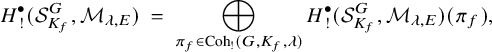(2.1) $$ \begin{align} H^{\bullet}_{\,!}(\mathcal{S}^G_{K_f}, \mathcal{M}_{\lambda,E}) \ =\ \bigoplus_{\pi_f \in \mathrm{Coh}_!(G,K_f,\lambda)} H^{\bullet}_{\,!}(\mathcal{S}^G_{K_f}, \mathcal{M}_{\lambda,E})(\pi_f), \end{align} $$

where $\pi _f$ is an isomorphism type of an absolutely irreducible $\mathcal {H}^G_{K_f}$ -module (i.e., there is an E-vector space $V_{\pi _f}$ with an absolutely irreducible action $\pi _f$ of $\mathcal {H}^G_{K_f}$ ). Let $\mathcal {H}^G_{K_p} = C^\infty _c(G(\mathbb {Q}_p)/ \! \!/K_p)$ be the local Hecke-algebra. The local factors $\mathcal {H}^G_{K_p}$ are commutative outside a finite set $\mathrm {S} = \mathrm {S}_{K_f}$ of primes and the factors for two different primes commute with each other. For $p \not \in \mathrm {S}$ , the commutative algebra $\mathcal {H}^G_{K_p}$ acts on $V_{\pi _f} $ by a homomorphism $\pi _p : \mathcal {H}^G_{K_p} \to E.$ Let $V_{\pi _p}$ be the one-dimensional E-vector space E with the distinguished basis element $1\in E$ and with the action $\pi _p$ on it. Then $V_{\pi _f} \ = \ V_{\pi _f,\mathrm {S}} \otimes \otimes ^\prime _{p\not \in \mathrm {S}} V_{\pi _p} \ = \ \otimes _{p\in \mathrm {S}} V_{\pi _p}\otimes E,$ where the absolutely-irreducible $\mathcal {H}^G_{K_f,\mathrm {S}}$ -module $ V_{\pi _f,\mathrm {S}}$ module is decomposed as a tensor product $V_{\pi _f,\mathrm {S}}= \otimes _{p\in \mathrm {S}}V_{\pi _p}$ of absolutely irreducible $\mathcal {H}^G_{K_p}$ -modules. The Hecke algebra decomposes as $\mathcal {H}^G_{K_f}\ = \ \mathcal {H}^G_{K_f,\mathrm {S}}\times \otimes _{p\not \in \mathrm {S}}\mathcal {H}^G_{K_p} \ = \ \mathcal {H}^G_{K_f,\mathrm {S}} \times \mathcal {H}^{G,\mathrm {S}},$ where the first factor acts on the first factor $V_{\pi _f, \mathrm {S}}$ and the second factor acts via the homomorphism $\pi _f^{\mathrm {S}} : \mathcal {H}^{G,\mathrm {S}} \to E.$ The set ${\mathrm {Coh}}_!(G, K_f, \lambda )$ of isomorphism classes which occur with strictly positive multiplicity in (2.1) is called the inner spectrum of G with $\lambda $ -coefficients and level structure $K_f.$ Taking the union over all $K_f$ , the inner spectrum of G with $\lambda $ -coefficients is defined to be ${\mathrm {Coh}}_!(G, \lambda ) \ = \ \bigcup _{K_f} {\mathrm {Coh}}_!(G, K_f, \lambda ). $ Since the inner spectrum is captured, at a transcendental level, by the cohomology of the discrete spectrum, it follows from the strong multiplicity one theorem for the discrete spectrum for $\mathrm {{GL}}_n$ (see Jacquet [31] and Mœglin–Waldspurger [39]) that $\pi _f$ is determined by its restriction $\pi _f^{\mathrm {S}}$ to the central subalgebra $\mathcal {H}^{G,\mathrm {S}}$ of $\mathcal {H}^G_{K_f}.$

2.2 Cuspidal cohomology

Take $E = \mathbb {C}$ and consider $\lambda \in X^+_{\mathrm {alg}}(T \times \mathbb {C}).$ Denote $\mathfrak {g}_\infty $ (resp., $\mathfrak {k}_\infty $ ) the Lie algebra of $G(\mathbb {R})$ (resp., of $K_\infty = C_\infty S(\mathbb {R}).$ ) The cohomology $H^{\bullet }(\mathcal {S}^G_{K_f},\widetilde {\mathcal {M}}_{\lambda , \mathbb {C}})$ is the cohomology of the de Rham complex denoted $\Omega ^{\bullet }(\mathcal {S}^G_{K_f}, \widetilde {\mathcal {M}}_{\lambda , \mathbb {C}}).$ The de Rham complex is isomorphic to the relative Lie algebra complex

$$ \begin{align*}\Omega^{\bullet}(\mathcal{S}^G_{K_f}, \widetilde{\mathcal{M}}_{\lambda, \mathbb{C}} ) \ = \ \mathrm{{Hom}}_{K_\infty} (\Lambda^{\bullet}(\mathfrak{g}_\infty/\mathfrak{k}_\infty), \, \mathcal{C}^\infty(G(\mathbb{Q})\backslash G(\mathbb{A})/K_f, \omega_{\lambda}^{-1}|_{S(\mathbb{R})^0}) \otimes \mathcal{M}_{\lambda, \mathbb{C}}), \end{align*} $$

where $\mathcal {C}^\infty (G(\mathbb {Q})\backslash G(\mathbb {A})/K_f, \omega _{\lambda }^{-1}|_{S(\mathbb {R})^0})$ consists of all smooth functions $\phi : G(\mathbb {A}) \to \mathbb {C}$ such that $\phi (a \, \underline g \, \underline k_f \, s_\infty ) = \omega _{\lambda }^{-1}(s_\infty ) \phi (\underline g),$ for all $a \in G(\mathbb {Q})$ , $\underline g \in G(\mathbb {A})$ , $\underline k_f \in K_f$ and $s_\infty \in S(\mathbb {R})^0.$ Abbreviating $\omega _{\lambda }^{-1}|_{S(\mathbb {R})^0}$ as $\omega _\infty ^{-1},$ if $t \in \mathbb {R}_{>0} \cong S(\mathbb {R})^0$ , then $ \omega _{\lambda }(t) \ = \ t^{N \sum _{\tau : F \to \mathbb {C}} d^\tau } \ = \ t^{\sum _\tau \sum _i b_i^\tau }.$ The identification of the complexes gives an identification between our basic object of interest over $\mathbb {C}$ with the relative Lie algebra cohomology of the space of smooth automorphic forms twisted by the coefficient system:

$$ \begin{align*}H^{\bullet}(\mathcal{S}^G_{K_f}, \widetilde{\mathcal{M}}_{\lambda,\mathbb{C}}) \ = \ H^{\bullet}(\mathfrak{g}_\infty, \mathfrak{k}_\infty; \mathcal{C}^\infty(G(\mathbb{Q})\backslash G(\mathbb{A})/K_f, \omega_{\lambda}^{-1}|_{S(\mathbb{R})^0}) \otimes \mathcal{M}_{\lambda, \mathbb{C}}). \end{align*} $$

The inclusion $\mathcal {C}_{\mathrm {cusp}}^\infty (G(\mathbb {Q})\backslash G(\mathbb {A})/K_f, \omega _\infty ^{-1}) \subset \mathcal {C}^\infty (G(\mathbb {Q})\backslash G(\mathbb {A})/K_f, \omega _\infty ^{-1}),$ of the space of smooth cusp forms, induces an inclusion in relative Lie algebra cohomology (due to Borel [2]), and cuspidal cohomology is defined as

$$ \begin{align*}H_{\mathrm{cusp}}^{\bullet}(\mathcal{S}^G_{K_f}, \widetilde{\mathcal{M}}_{\lambda, \mathbb{C}}) \ := \ H^{\bullet} \left(\mathfrak{g}_\infty, \mathfrak{k}_\infty; \, \mathcal{C}^\infty_{\mathrm{cusp}}(G(\mathbb{Q})\backslash G(\mathbb{A})/K_f, \omega_\infty^{-1}) \otimes \mathcal{M}_\lambda \right). \end{align*} $$

Furthermore, $H_{\mathrm {cusp}}^{\bullet }(\mathcal {S}^G_{K_f}, \mathcal {M}_{\lambda , \mathbb {C}}) \subset H_{!}^{\bullet }(\mathcal {S}^G_{K_f}, \mathcal {M}_{\lambda , \mathbb {C}}).$ Define $\mathrm {{Coh}}_{\mathrm {cusp}}(G,\lambda ,K_f)$ as the set of all $\pi _f \in \mathrm {{Coh}}_!(G, \lambda ,K_f)$ which contribute to cuspidal cohomology. The decomposition of cuspforms into cuspidal automorphic representations gives the following fundamental decomposition for cuspidal cohomology:

(2.2) $$ \begin{align} H_{\mathrm{cusp}}^{\bullet}(\mathcal{S}^G_{K_f}, \widetilde{\mathcal{M}}_{\lambda, \mathbb{C}}) \ := \ \bigoplus_{\pi \in \mathrm{{Coh}}_{\mathrm{cusp}}(G,\lambda,K_f)} H^{\bullet}(\mathfrak{g}_\infty, \mathfrak{k}_\infty; \pi_\infty \otimes \mathcal{M}_{\lambda, \mathbb{C}}) \otimes \pi_f. \end{align} $$

To clarify a slight abuse of notation: if a cuspidal automorphic representation $\pi $ contributes to the above decomposition, then its representation at infinity is $\pi _\infty $ (which admits an explicit description that will be crucial for all the archimedean calculations), and $\pi _f$ denotes the $K_f$ -invariants of its finite part. The level structure $K_f$ will be clear from context; hence whether $\pi _f$ denotes the finite-part or its $K_f$ -invariants will be clear from context. Define ${\mathrm {Coh}}_{\mathrm {cusp}}(G, \lambda ) \ = \ \bigcup _{K_f} {\mathrm {Coh}}_{\mathrm {cusp}}(G, K_f, \lambda ).$

2.3 Pure weights and strongly-pure weights

2.3.1 Strongly-pure weights over $\mathbb {C}$

If a weight $\lambda = (\lambda ^\eta )_{\eta :F \to \mathbb {C}} \in X^+_{\mathrm {alg}}(T \times \mathbb {C})$ supports cuspidal cohomology (i.e., if $H_{\mathrm {cusp}}^{\bullet }(\mathcal {S}^G_{K_f}, \widetilde {\mathcal {M}}_{\lambda , \mathbb {C}}) \neq 0$ ), then $\lambda $ satisfies the purity condition

(2.3) $$ \begin{align} a_i^\eta = a_{N-i}^{\bar{\eta}} \ \mbox{for all } \eta : F \to \mathbb{C}\ \iff \ \exists \,\mathbf{{w}} \mbox{ such that } b^\eta_i + b^{\bar{\eta}}_{N-i+1} = \mathbf{{w}} \text{ for all } \eta \text{ and } i, \end{align} $$

which follows from the purity lemma [7, Lem. 4.9]. The integer $\mathbf {{w}}$ is called the purity weight of $\lambda .$ The weight $\lambda $ is said to be pure if it satisfies (2.3), and denote by $X^+_{0}(T \times \mathbb {C})$ the set of all such pure weights. Next, recall a theorem of Clozel that says that cuspidal cohomology for $\mathrm {{GL}}_N/F$ admits a rational structure [7, Thm. 3.19], from which it follows that any $\varsigma \in \mathrm {{Aut}}(\mathbb {C})$ stabilizes cuspidal cohomology, that is, ${}^\varsigma \lambda $ also satisfies the above purity condition, where if $\lambda = (\lambda ^\eta )_{\eta : F \to \mathbb {C}}$ and $\varsigma \in \mathrm {{Aut}}(\mathbb {C})$ , then ${}^\varsigma \lambda $ is the weight $({}^\sigma \lambda ^\eta )_{\eta : F \to \mathbb {C}}$ where ${}^\varsigma \lambda ^\eta = \lambda ^{\varsigma ^{-1}\circ \eta }$ . A pure weight $\lambda $ will be called strongly-pure if ${}^\varsigma \lambda $ is pure with purity-weight $\mathbf {{w}}$ for every $\varsigma \in \mathrm {{Aut}}(\mathbb {C});$ denote by $X^+_{00}(T \times \mathbb {C})$ the set of all such strongly-pure weights. For $\lambda \in X^+_{00}(T \times \mathbb {C}),$ note that

$$ \begin{align*}b^{\varsigma^{-1} \circ \eta}_j + b^{\varsigma^{-1} \circ \overline{\eta}}_{N-j+1} = \mathbf{{w}}, \ \mbox{for all} \ 1 \leq j \leq N, \ \eta : F \to \mathbb{C}, \ \varsigma \in \mathrm{{Aut}}(\mathbb{C}). \end{align*} $$

We have the following inclusions inside the character group of $T \times \mathbb {C},$ which are all, in general, strict inclusions:

$$ \begin{align*}X^+_{00}(T \times \mathbb{C}) \ \subset \ X^+_{0}(T \times \mathbb{C}) \ \subset \ X^+_{\mathrm{alg}}(T \times \mathbb{C}) \ \subset \ X^+(T \times \mathbb{C}) \ \subset \ X^{*}(T \times \mathbb{C}). \end{align*} $$

2.3.2 Strongly-pure weights over E

The set of strongly-pure weights may be defined at an arithmetic level. Recall the standing assumption on E that is a finite Galois extension of $\mathbb {Q}$ that takes a copy of F; in particular, any embedding $\iota : E \to \mathbb {C}$ factors as $\iota : E \to \bar {\mathbb {Q}} \subset \mathbb {C}.$ Furthermore, $\iota : E \to \mathbb {C}$ gives a bijection $\iota _* : \mathrm {{Hom}}(F,E) \to \mathrm {{Hom}}(F,\mathbb {C})$ as $\iota _*(\tau ) = \iota \circ \tau $ , which in turn gives a bijection $X^{*}(T \times E) \to X^{*}(T \times \mathbb {C})$ that maps $\lambda = (\lambda ^\tau )_{\tau : F \to E}$ to ${}^\iota \lambda = ({}^\iota \lambda ^\eta )_{\eta : F \to \mathbb {C}} = (\lambda ^{\iota ^{-1} \circ \eta })_{\eta : F \to \mathbb {C}}.$

Proposition 2.4. Let $\lambda \in X^+_{\mathrm {alg}}(T \times E)$ be an algebraic dominant integral weight. Suppose $\lambda = (\lambda ^\tau )_{\tau : F \to E}$ with $\lambda ^\tau = (b^\tau _1 \geq \cdots \geq b^\tau _N)$ . Then, the following are equivalent:

1. (i) There exists $\iota : E \to \mathbb {C}$ such that ${}^\iota \lambda \in X^+_{00}(T \times \mathbb {C})$ ; that is, for every $\gamma \in \mathrm {{Gal}}(\bar {\mathbb {Q}}/\mathbb {Q})$ , we have ${}^{\gamma \circ \iota }\lambda \in X^+_{0}(T \times \mathbb {C})$ with the same purity weight:

   $$ \begin{align*} \text{"}\exists \, \iota : E \to \mathbb{C}, \ \exists \, \mathbf{{w}} \in \mathbb{Z} \ \ \mbox{such that} \ \ b_j^{\iota^{-1}\circ \gamma^{-1} \circ \eta} &+ b_{N-j+1}^{\iota^{-1}\circ \gamma^{-1} \circ \bar{\eta}} \ = \ \mathbf{{w}}, \\ &\qquad \forall \gamma \in \mathrm{{Gal}}(\bar{\mathbb{Q}}/\mathbb{Q}), \ \forall \eta : F \to \mathbb{C}, \ 1 \leq j \leq N.\text{"} \end{align*} $$

2. (ii) For every $\iota : E \to \mathbb {C}$ , ${}^\iota \lambda \in X^+_{00}(T \times \mathbb {C})$ , that is, for every $\gamma \in \mathrm {{Gal}}(\bar {\mathbb {Q}}/\mathbb {Q})$ , we have ${}^{\gamma \circ \iota }\lambda \in X^+_{00}(T \times \mathbb {C})$ with the same purity weight:

   $$ \begin{align*} \text{"}\exists\, \mathbf{{w}} \in \mathbb{Z} \ \ \mbox{such that} \ \ b_j^{\iota^{-1}\circ \gamma^{-1} \circ \eta} &+ b_{N-j+1}^{\iota^{-1}\circ \gamma^{-1} \circ \bar{\eta}} \ = \ \mathbf{{w}}, \\ &\quad \forall \, \iota : E \to \mathbb{C}, \ \forall\, \gamma \in \mathrm{{Gal}}(\bar{\mathbb{Q}}/\mathbb{Q}), \ \forall\, \eta : F \to \mathbb{C}, \ 1 \leq j \leq N.\text{"} \end{align*} $$

3. (iii) For every $\iota : E \to \mathbb {C}$ , ${}^\iota \lambda \in X^+_{0}(T \times \mathbb {C})$ with the same purity weight,

   $$ \begin{align*}\text{"}\exists\, \mathbf{{w}} \in \mathbb{Z} \ \ \mbox{such that} \ \ b_j^{\iota^{-1}\circ \eta} + b_{N-j+1}^{\iota^{-1}\circ \bar{\eta}} \ = \ \mathbf{{w}}, \ \forall \, \iota : E \to \mathbb{C}, \ \forall\, \eta : F \to \mathbb{C}, \ 1 \leq j \leq N.\text{"} \end{align*} $$

Proof. Fix $\iota _0 : E \to \mathbb {C}$ . Since $E/\mathbb {Q}$ is a finite Galois extension, the inclusions

$$ \begin{align*}\{\gamma \circ \iota_0 \ | \ \gamma \in \mathrm{{Gal}}(\bar{\mathbb{Q}}/\mathbb{Q})\} \ \subset \ \{\gamma \circ \iota \ | \ \gamma \in \mathrm{{Gal}}(\bar{\mathbb{Q}}/\mathbb{Q}), \iota : E \to \mathbb{C}\} \ \subset \ \mathrm{{Hom}}(E,\mathbb{C}) \end{align*} $$

are all equalities.

The set of strongly-pure weights over E, denoted $X^+_{00}(T \times E)$ , consists of the algebraic dominant integral weights $\lambda \in X^{*}(T \times E)$ that satisfy any one, and hence all, of the conditions in the above proposition. It is most convenient to work with the characterization in $(iii)$ . There are the following inclusions within the character group of $T \times E$ , which are all, in general, strict inclusions:

$$ \begin{align*}X^+_{00}(T \times E) \ \subset \ X^+_{\mathrm{alg}}(T \times E) \ \subset \ X^+(T \times E) \ \subset \ X^{*}(T \times E). \end{align*} $$

The existence of a strongly-pure weight over a totally imaginary base field F depends on the internal structure of F; this is explained over the course of the next four paragraphs.

2.3.3 Interlude on (strongly-)pure weights for a CM field

When the base field F is a CM field, then a pure weight is also strongly-pure. Given any $\varsigma \in \mathrm {{Aut}}(\mathbb {C})$ , one can check that $\varsigma _*(X^+_{0}(T \times \mathbb {C})) \ = \ X^+_{0}(T \times \mathbb {C}).$

Lemma 2.5. Let $\eta : F \to \mathbb {C}$ and $\varsigma : \mathbb {C} \to \mathbb {C}$ be field homomorphisms, and let ${\mathfrak {c}} : \mathbb {C} \to \mathbb {C}$ stand for complex conjugation. Then

$$ \begin{align*}\varsigma \circ {\mathfrak{c}} \circ \eta \ = \ {\mathfrak{c}} \circ \varsigma \circ \eta, \end{align*} $$

that is, complex conjugation and any automorphism of $\mathbb {C}$ commute on the image of a CM field.

Proof. Let $\eta _1 = \varsigma \circ {\mathfrak {c}} \circ \eta $ and $\eta _2 = {\mathfrak {c}} \circ \varsigma \circ \eta .$ Then $\eta _1|_{F^+} = \eta _2|_{F^+}$ (recall that $F^+$ is the maximal totally real subfield of F). This means that $\eta _1 = \eta _2$ or $\eta _1 = {\mathfrak {c}} \circ \eta _2$ ; if the latter, then $\varsigma \circ {\mathfrak {c}} \circ \eta = \varsigma \circ \eta $ . Evaluate both sides on $x \in F - F^+$ on which ${\mathfrak {c}}(\eta (x)) = -\eta (x)$ to get a contradiction.

Let $\lambda = (\lambda ^\eta )_{\eta : F \to \mathbb {C}} \in X^+_{0}(T \times \mathbb {C})$ ; hence, $d^\eta + d^{\bar {\eta }} = \mathbf {{w}}$ for all $\eta : F \to \mathbb {C}.$ Take any $\varsigma \in \mathrm {{Aut}}(\mathbb {C})$ and consider ${}^\varsigma \lambda $ ; to see its purity, note that

$$ \begin{align*}b_{j}^{\varsigma^{-1} \circ \eta} + b_{N-j+1}^{\varsigma^{-1} \circ \bar{\eta}} \ = \ b_{j}^{\varsigma^{-1} \circ \eta} + b_{N-j+1}^{\varsigma^{-1} \circ {\mathfrak{c}} \circ \eta} \ = \ b_{j}^{\varsigma^{-1} \circ \eta} + b_{N-j+1}^{{\mathfrak{c}} \circ \varsigma^{-1} \circ \eta} \ = \ b_{j}^{\varsigma^{-1} \circ \eta} + b_{N-j+1}^{\overline{\varsigma^{-1} \circ \eta}} = \mathbf{{w}}, \end{align*} $$

where the second equality is from Lemma 2.5 above. Hence, $\lambda $ is strongly-pure.

2.3.4 Interlude on strongly-pure weights for a general totally imaginary field

When F is totally imaginary but not CM, there may exist weights that are pure but not strongly-pure. The following example is instructive: take $F = \mathbb {Q}(2^{1/3},\omega ),$ where $2^{1/3}$ is the real cube root of $2$ and $\omega = e^{2\pi i/3}.$ Then $\Sigma _F = \mathrm {{Gal}}(F/\mathbb {Q}) \simeq S_3$ the permutation group in 3 letters taken to be $\{2^{1/3}, \, 2^{1/3}\omega , \, 2^{1/3}\omega ^2\}.$ Let $s \in S_3$ correspond to $\eta _s : F \to \mathbb {C}.$ Consider the weights $\lambda = (\lambda ^{\eta _s})_{s \in S_3}$ and $\mu = (\mu ^{\eta _s})_{s \in S_3}$ for $\mathrm {Res}_{F/\mathbb {Q}}(\mathrm {{GL}}(1)/F)$ described in the table:

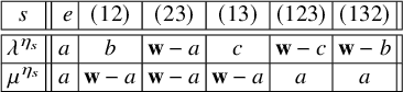$$ \begin{align*} \begin{array}{|c||c|c|c|c|c|c||} \hline s & \ e \ & (12) & (23) & (13) & (123) & (132) \\ \hline \hline \lambda^{\eta_s} & a & b & \mathbf{{w}}-a & c & \mathbf{{w}}-c & \mathbf{{w}}-b \\ \hline \mu^{\eta_s} & a & \mathbf{{w}}-a & \mathbf{{w}}-a & \mathbf{{w}}-a & a & a \\ \hline \end{array} \end{align*} $$

where $a,b,c,\mathbf {{w}} \in \mathbb {Z}$ . For the tautological embedding $F \subset \mathbb {C},$ the set $\Sigma _F$ is paired into complex conjugates as $\{(\eta _{e}, \eta _{(23)}), (\eta _{(12)}, \eta _{(132)}), (\eta _{(13)}, \eta _{(123)})\},$ from which it follows that $\lambda $ is a pure weight. All other possible pairings of $\Sigma _F$ into conjugates via automorphisms of $\mathbb {C}$ are given by: $\{(\eta _{e}, \eta _{(12)}), (\eta _{(23)}, \eta _{(123)}), (\eta _{(13)}, \eta _{(132)})\},$ and $\{(\eta _{e}, \eta _{(13)}), (\eta _{(23)}, \eta _{(132)}), (\eta _{(12)}, \eta _{(123)})\};$ (F being Galois this simply boils down to composing these embeddings $\eta _s$ by a fixed one $\eta _{s_0},$ and using $\eta _{s_0} \circ \eta _{s} = \eta _{s_0s}$ ). It follows that $\lambda $ is not strongly-pure if $\mathbf {{w}}-a, b$ and c are not all equal, but $\mu $ is strongly-pure and has purity weight $\mathbf {{w}}.$

2.3.5 On the internal structure of a general totally imaginary field

Let F be a totally imaginary field as before. Let $F_0$ be the largest totally real subfield in F. Then there is at most one totally imaginary quadratic extension $F_1$ of $F_0$ inside F. (See, for example, Weil [51].) If $\alpha $ and $\beta $ are two totally negative elements of $F_0$ giving two possible such extensions $F_0(\sqrt {\alpha })$ and $F_0(\sqrt {\beta })$ , then by maximality of $F_0$ , one has $\sqrt {\alpha \beta } \in F_0$ , that is, $\alpha = t^2 \beta $ for $t \in F_0$ , whence $F_0(\sqrt {\alpha }) = F_0(\sqrt {\beta }).$ There are two distinct cases to consider:

1. (i) CM: when there is indeed such an imaginary quadratic extension $F_1$ of $F_0$ , then $F_1$ is the maximal CM subfield of F; of course, $[F_1:F_0] = 2$ . For example, if $F = \mathbb {Q}(2^{1/3},\omega )$ as in 2.3.4, then $F_0 = \mathbb {Q}$ and $F_1 = \mathbb {Q}(\omega )$ .

2. (ii) TR: when there is no imaginary quadratic extension of $F_0$ inside F, then put $F_1 = F_0$ for the maximal totally real subfield of F. For example, take $F_0$ to be a cubic totally real field (e.g., $F_0 = \mathbb {Q}(\zeta _7+\zeta _7^{-1})$ , $\zeta _7 = e^{2\pi i/7}$ ), and take non-square elements $a,b \in F_0$ whose conjugates $a,a',a"$ and $b,b',b"$ are such that $a>0, \ a'<0, a"<0$ and $b<0, \ b'<0,\ b">0$ ; such a and b exist by weak-approximation; take $F = F_0(\sqrt {a}, \sqrt {b})$ . Then there is no intermediate CM-subfield between $F_0$ and F; hence, $F_1 = F_0.$

As will be explained later on, that in case TR, asking for a critical point for a Rankin–Selberg L-function for $\mathrm {{GL}}(n) \times \mathrm {{GL}}(n')/F$ will impose the restriction $nn'$ is even. This should not be surprising because, as is well-known, for an algebraic Hecke character $\chi $ over F, if the L-function $L(s,\chi )$ has critical points, then that forces us to be in case CM (see [42]).

Notation in the CM-case.

Suppose $\mathrm {S}_\infty (F)$ (resp., $\mathrm {S}_\infty (F_1)$ ) is the set of archimedean places of F (resp., $F_1$ ). Enumerate $\mathrm {S}_\infty (F_1)$ as $\{w_1,\dots , w_{\mathrm r_1}\}$ , where ${\mathrm r}_1 = d_{F_1}/2 = [F_1:\mathbb {Q}]/2.$ For $ 1 \leq j \leq {\mathrm r}_1$ , let $\{\nu _j, \bar \nu _j\} \subset \Sigma _{F_1}$ be the pair of conjugate embeddings corresponding to $w_j;$ the non-canonical choice of $\nu _j$ is fixed and is distinguished in the sense that $\nu _j$ induces the isomorphism $F_{1,w_j} \simeq \mathbb {C}.$ Let $k = [F:F_1].$ Let $v_{j1},\dots ,v_{jk}$ be the set of places in $\mathrm {S}_\infty (F)$ above $w_j.$ Let $\varrho : \Sigma _F \to \Sigma _{F_1}$ denote the restriction map $\varrho (\eta ) = \eta |_{F_1}.$ Suppose $\varrho ^{-1}(\nu _j) = \{\eta _{j1},\dots , \eta _{jk}\}$ . Then $\varrho ^{-1}(\bar \nu _j) = \{\bar {\eta }_{j1},\dots , \bar {\eta }_{jk}\},$ with the indexing being such that the pair of conjugate embeddings $\{\eta _{jl}, \bar {\eta }_{jl}\}$ corresponds to $v_{jl} \in \mathrm {S}_\infty (F)$ for all $1 \leq j \leq {\mathrm r}_1$ and $1 \leq l \leq k.$

Notation in the TR-case.

Let $\mathrm {S}_\infty (F_1) = \{w_1,\dots , w_{d_{F_1}}\}$ be an enumeration of the set of archimedean places of $F_1$ , where $d_{F_1} = [F_1:\mathbb {Q}];$ since $F_1$ is the maximal totally real subfield of the totally imaginary F, the degree $d_{F_1}$ can be either even or odd, but the index $k = [F:F_1]$ is even; suppose $k = 2k_1.$ For $ 1 \leq j \leq d_{F_1}$ , let $\nu _j \in \Sigma _{F_1}$ be complex embedding corresponding to $w_j.$ As before, $\varrho : \Sigma _F \to \Sigma _{F_1}$ denotes the restriction map $\varrho (\eta ) = \eta |_{F_1}.$ Let $v_{j1},\dots ,v_{jk_1}$ be the set of places in $\mathrm {S}_\infty (F)$ above $w_j$ , and suppose $v_{ji}$ corresponds to the pair of conjugate embeddings $\{\eta _{ji}, \bar {\eta }_{ji}\}$ . Then $\varrho ^{-1}(\nu _j) = \{\eta _{j1}, \bar {\eta }_{j1}, \eta _{j2}, \bar {\eta }_{j2}, \dots , \eta _{jk_1}, \bar {\eta }_{jk_1}\}$ .

2.3.6 Strongly-pure weights over F are base-change from $F_1$

Proposition 2.6. Suppose $\lambda \in X^+_{00}(\mathrm {Res}_{F/\mathbb {Q}}(T_{N,0}) \times E)$ is a strongly-pure weight. Then there exists $\kappa \in X^+_{00}(\mathrm {Res}_{F_1/\mathbb {Q}}(T_{N,0}) \times E)$ such that $\lambda $ is the base-change of $\kappa $ from $F_1$ to F in the sense that for any $\tau : F \to E$ , $\lambda ^\tau = \kappa ^{\tau |_{F_1}}.$

For brevity, the conclusion will be denoted as $\lambda = \mathrm {BC}_{F/F_1}(\kappa ).$

Proof. It suffices to prove the proposition over $\mathbb {C}$ , that is, if $'\lambda \in X^+_{00}(\mathrm {Res}_{F/\mathbb {Q}}(T_{N,0}) \times \mathbb {C})$ , then it suffices to show the existence $'\kappa \in X^+_{00}(\mathrm {Res}_{F_1/\mathbb {Q}}(T_{N,0}) \times \mathbb {C})$ such that $'\lambda = \mathrm { BC}_{F/F_1}('\kappa );$ because, then given the $\lambda $ in the proposition, take an embedding $\iota : E \to \mathbb {C}$ , and let $'\lambda = {}^\iota \lambda $ , to which using the statement over $\mathbb {C}$ one gets $'\kappa $ , which defines a unique $\kappa $ via ${}^\iota \kappa = {}'\kappa .$ It is clear that $\lambda = \mathrm {BC}_{F/F_1}(\kappa )$ because this is so after applying $\iota $ .

To prove the statement over $\mathbb {C}$ , take $\lambda \in X^+_{00}(\mathrm {Res}_{F/\mathbb {Q}}(T_{N,0}) \times \mathbb {C})$ , and suppose $\lambda = (\lambda ^\eta )_{\eta : F \to \mathbb {C}}$ with $\lambda ^\eta = (b^\eta _1 \geq b^\eta _2 \geq \cdots \geq b^\eta _N).$ Strong-purity gives

$$ \begin{align*}b^{\gamma \circ \eta}_{N-j+1} + b^{\gamma \circ \bar{\eta}}_j = \mathbf{{w}}, \quad \forall \gamma \in \mathrm{{Gal}}(\bar{\mathbb{Q}}/\mathbb{Q}), \ \forall \eta \in \Sigma_F, \ 1 \leq j \leq N. \end{align*} $$

Also, one has

$$ \begin{align*}b^{\gamma \circ \eta}_{N-j+1} + b^{\overline{\gamma \circ \eta}}_j = \mathbf{{w}}, \quad \forall \gamma \in \mathrm{{Gal}}(\bar{\mathbb{Q}}/\mathbb{Q}), \ \forall \eta \in \Sigma_F, \ 1 \leq j \leq N. \end{align*} $$

Hence, we get $b^{\gamma \circ \bar {\eta }}_j \ = \ b^{\overline {\gamma \circ \eta }}_j.$ Exactly as explicated in the proof of Proposition 26 in [42], one gets $b^{\gamma \circ \eta }_j = b^{\eta }_j$ for all $\gamma $ in the normal subgroup of $\mathrm {{Gal}}(\bar {\mathbb {Q}}/\mathbb {Q})$ generated by the commutators $\{g {\mathfrak {c}} g^{-1} {\mathfrak {c}} : g \in \mathrm {{Gal}}(\bar {\mathbb {Q}}/\mathbb {Q})\}$ , and all $\eta : F \to \mathbb {C}.$ This means that $b^{\eta }_j$ depends only on $\eta |_{F_1}.$

2.4 Strongly inner cohomology

The problem of giving an arithmetic characterization of cuspidal cohomology is addressed in [27, Chap. 5] in great detail for $\mathrm {{GL}}_N$ over a totally real field. In this article, for $\mathrm {{GL}}_N$ over a totally imaginary F, we will only discuss it en passant and contend ourselves in making the following:

Definition 2.7. Take a field E large enough (as before), and let $\lambda \in X^+_{00}(T \times E).$ The strongly inner spectrum of $\lambda $ for level structure $K_f$ is defined as

$$ \begin{align*} \mathrm{{Coh}}_{!!}&(G, K_f, \lambda) \ = \\ &\qquad\qquad \{\pi_f \in \mathrm{{Coh}}_!(G, K_f, \lambda) \ : \ {}^\iota\pi_f \in \mathrm{{Coh}}_{\mathrm{cusp}}(G, K_f, {}^\iota\lambda) \text{ for some embedding } \iota : E \to \mathbb{C}\}. \end{align*} $$

An irreducible Hecke-summand $\pi _f$ in inner cohomology is strongly-inner if under some embedding $\iota $ rendering the context transcendental, it contributes to cuspidal cohomology. The point of view in loc.cit. is that the definition is independent of $\iota $ , and hence giving a rational origin (i.e., over E) to cuspidal summands giving another proof of a result of Clozel that cuspidal cohomology for $\mathrm {{GL}}_N$ admits a rational structure [7, Thm. 3.19]. In this article, one simply appeals to Clozel’s theorem to observe that the definition of strongly inner spectrum is independent of the choice of embedding $\iota $ ; that is, if $\iota , \iota ' : E \to \mathbb {C}$ are two such embeddings, then

$$ \begin{align*}{}^\iota\pi_f \in \mathrm{{Coh}}_{\mathrm{cusp}}(G, {}^\iota\lambda) \ \iff \ {}^{\iota'}\!\pi_f \in \mathrm{{Coh}}_{\mathrm{cusp}}(G, {}^{\iota'}\!\lambda). \end{align*} $$

Define strongly-inner cohomology as

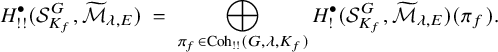$$ \begin{align*}H_{!!}^{\bullet}(\mathcal{S}^G_{K_f}, \widetilde{\mathcal{M}}_{\lambda, E}) \ = \ \bigoplus_{\pi_f \in \mathrm{{Coh}}_{!!}(G,\lambda,K_f)} H_{!}^{\bullet}(\mathcal{S}^G_{K_f}, \widetilde{\mathcal{M}}_{\lambda, E})(\pi_f). \end{align*} $$

Then, since cuspidal cohomology is contained in inner cohomology, it is clear that

$$ \begin{align*}H_{!!}^{\bullet}(\mathcal{S}^G_{K_f}, \widetilde{\mathcal{M}}_{\lambda, E}) \otimes_{E,\iota} \mathbb{C} \ \simeq \ H_{\mathrm{cusp}}^{\bullet}(\mathcal{S}^G_{K_f}, \widetilde{\mathcal{M}}_{{}^\iota\!\lambda, \mathbb{C}}). \end{align*} $$

For $\lambda \in X^+_{00}(T \times E)$ , $\pi _f \in \mathrm {{Coh}}_{!!}(G, \lambda )$ (ignoring the level structure) and $\iota : E \to \mathbb {C}$ , since ${}^\iota \pi _f \in \mathrm {{Coh}}_{\mathrm {cusp}}(G, {}^\iota \lambda )$ , let ${}^\iota \pi $ stand for the unique global cuspidal automorphic representation of $G(\mathbb {A}_{\mathbb {Q}}) = \mathrm {{GL}}_N(\mathbb {A}_F)$ whose finite part is $({}^\iota \pi )_f = {}^\iota \pi _f.$ The representation at infinity $({}^\iota \pi )_\infty ,$ to be denoted $\mathbb {J}_{{}^\iota \!\lambda }$ below, will be explicitly described in Section 2.5.

2.4.1 Tate twists

Let $m \in \mathbb {Z}.$ For $\lambda \in X^+(T_N \times E)$ , define by the rule that if $\lambda ^\tau = (b_1^\tau ,\dots , b_N^\tau )$ , then for $\tau : F \to E.$ It is clear that preserves each of the properties: dominant, integral, algebraic and (strongly-)pure. As in [27, Sect. 5.2.4], cupping with the m-th power of the fundamental class gives us an isomorphism that maps (strongly-)inner cohomology to (strongly-)inner cohomology, and suppose $\pi _f \in \mathrm {{Coh}}_{!!}(G,\lambda )$ . Then $T^{\bullet }_{\mathrm {Tate}}(m)(\pi _f) \ = \ \pi _f(-m),$ where, $\pi _f(-m)$ is defined by $\pi _f(-m)(g_f) = \pi _f(g_f) \otimes |\!|g_f|\!|^{-m}.$

2.5 Archimedean considerations

2.5.1 Cuspidal parameters and cohomological representations of $\mathrm {{GL}}_N(\mathbb {C})$

Given a weight $\lambda = (\lambda ^\eta )_{\eta :F \to \mathbb {C}} \in X^+_{00}(T \times \mathbb {C}),$ for each $v \in \mathrm {S}_\infty $ (recall that v corresponds to a pair of complex embeddings $\{\eta _v, \bar {\eta }_v\}$ of F into $\mathbb {C}$ , with $\eta _v$ used to identify $F_v$ with $\mathbb {C}$ ), define the cuspidal parameters of $\lambda $ at v by

$$ \begin{align*} \alpha^v \ := \ -w_0\lambda^{\eta_v} + \rho \ \ \mathrm{and} \ \ \beta^v \ := \ - \lambda^{\bar{\eta}_v} - \rho. \end{align*} $$

If $\lambda ^\eta = (b^\eta _1,\dots ,b^\eta _N)$ , then

(2.8) $$ \begin{align} \alpha^v \ = \ (\alpha^v_1, \dots, \alpha^v_N) \ = \ \left(-b^{\eta_v}_N+ \tfrac{(N-1)}{2}, \, -b^{\eta_v}_{N-1}+ \tfrac{(N-3)}{2}, \, \dots, \, -b^{\eta_v}_1 - \tfrac{(N-1)}{2}\right), \end{align} $$

and similarly,

(2.9) $$ \begin{align} \beta^v \ := \ (\beta^v_1, \dots, \beta^v_N) \ = \ \left(-b^{\bar{\eta}_v}_1 - \tfrac{(N-1)}{2}, \, -b^{\bar{\eta}_v}_2 - \tfrac{(N-3)}{2}, \, \dots, \, -b^{\bar{\eta}_v}_N + \tfrac{(N-1)}{2}\right). \end{align} $$

Purity implies that $\alpha ^v_j + \beta ^v_j = -\mathbf {{w}}.$ Define a representation of $\mathrm {{GL}}_N(F_v) \simeq \mathrm {{GL}}_N(\mathbb {C})$ as

(2.10) $$ \begin{align} \mathbb{J}_{\lambda_v} \ := \ \mathbb{J}(\lambda^{\eta_v}, \lambda^{\bar{\eta}_v}) \ := \ \mathrm{{Ind}}_{B_N(\mathbb{C})}^{\mathrm{{GL}}_N(\mathbb{C})} \left(z^{\alpha^v_1} \bar{z}^{\beta^v_1} \otimes \cdots \otimes z^{\alpha^v_N} \bar{z}^{\beta^v_N} \right), \end{align} $$

where $B_N$ is the subgroup of all upper-triangular matrices in $\mathrm {{GL}}_N,$ and by $\mathrm {{Ind}}$ we mean normalized (i.e., unitary) parabolic induction. Now define a representation of $G(\mathbb {R}) = \prod _v \mathrm {{GL}}_N(F_v)$ :

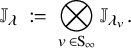(2.11) $$ \begin{align} \mathbb{J}_{\lambda} \ := \ \bigotimes_{v \in \mathrm{S}_\infty} \mathbb{J}_{\lambda_v}. \end{align} $$

Remark 2.12. Recall that the choice of the embedding $\eta _v$ in the pair $\{\eta _v, \bar {\eta }_v\}$ was fixed. If the roles of the $\eta _v$ and $\bar {\eta }_v$ are reversed, then it is easy to see that the pair $(\alpha ^v, \beta ^v)$ of cuspidal parameters would be replaced by $(w_0\beta ^v, w_0\alpha ^v)$ , whence, the representation $\mathbb {J}_v$ is replaced by its conjugate $\bar {\mathbb {J}}_v$ . See 2.5.2 below.

Some basic properties of $\mathbb {J}_\lambda $ are described in the following two propositions.

Proposition 2.13. Let $\lambda \in X^+_{00}(T \times \mathbb {C})$ and $\mathbb {J}_\lambda $ as above. Then

1. 1. $\mathbb {J}_\lambda $ is an irreducible essentially tempered representation admitting a Whittaker model.

2. 2. $H^{\bullet }(\mathfrak {g}, K_\infty; \, \mathbb {J}_\lambda \otimes \mathcal {M}_{\lambda , \mathbb {C}}) \neq 0.$

3. 3. Let $\mathbb {J}$ be an irreducible essentially tempered representation of $G(\mathbb {R}).$

   Suppose that $H^{\bullet }(\mathfrak {g}, K_\infty; \mathbb {J} \otimes \mathcal {M}_{\lambda , \mathbb {C}}) \neq 0$ then $\mathbb {J} = \mathbb {J}_\lambda .$

4. 4. If $\pi \in \mathrm {{Coh}}_{\mathrm {cusp}}(G,\lambda )$ (i.e., $\pi $ is a global cuspidal automorphic representation that contributes to cuspidal cohomology with respect to a strongly-pure weight $\lambda $ ), then $\pi _\infty \cong \mathbb {J}_\lambda .$

These are well-known results for $\mathrm {{GL}}_N(\mathbb {C})$ and are all easily seen from this elementary observation: for $z \in \mathbb {C}$ , let $|z|_{\mathbb {C}} = z \bar {z}$ ; then the representation

$$ \begin{align*}\mathbb{J}_{\lambda_v} \otimes |\ |_{\mathbb{C}}^{\mathbf{{w}}/2} \ = \ \mathrm{{Ind}}_{B_N(\mathbb{C})}^{\mathrm{{GL}}_N(\mathbb{C})} \left(z^{\alpha^v_1+ \mathbf{{w}}/2} \bar{z}^{\beta^v_1+\mathbf{{w}}/2} \, \otimes \, \cdots \, \otimes \, z^{\alpha^v_N+\mathbf{{w}}/2} \bar{z}^{\beta^v_N+\mathbf{{w}}/2} \right) \end{align*} $$

is unitarily induced from unitary characters (because of purity) and hence irreducible. A representation irreducibly induced from essentially discrete series representation is essentially tempered. Admitting a Whittaker model is a hereditary property. Nonvanishing of cohomology follows from Delorme’s Lemma (Borel–Wallach [5, Thm. III.3.3]), and that relative Lie algebra cohomology satisfies a Künneth theorem. Finally, among all representations with given infinitesimal character, there is at most one that is essentially tempered.

Define the following numbers:

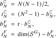(2.14) $$ \begin{align} \begin{aligned} b_N^{\mathbb{C}} & \ = \ N(N-1)/2, \\ t_N^{\mathbb{C}} & \ = \ (N^2-1) - b_N^{\mathbb{C}}, \\ b_N^F & \ = \ {\mathrm r} \cdot b_N^{\mathbb{C}}, \\ t_N^F & \ = \ \dim(\mathcal{S}^G) - b_N^F. \end{aligned} \end{align} $$

The relation between $b_N^F$ and $t_N^F$ is mitigated by an appropriate version of Poincaré duality, which is the reason why the ‘top-degree’ is defined in terms of the ‘bottom-degree’ and the dimension of the intervening symmetric space.

Proposition 2.15. Let $\lambda \in X^+_{00}(T \times \mathbb {C})$ and $\mathbb {J}_\lambda $ as above. Then

$$ \begin{align*}H^q(\mathfrak{g}, K_\infty; \, \mathbb{J}_{\lambda} \otimes \mathcal{M}_{\lambda, \mathbb{C}}) \neq 0 \ \ \iff \ \ b_N^F \ \leq \ q\ \leq \ t_N^F. \end{align*} $$

Furthermore, for extremal degrees $q \in \{b_N^F, \, t_N^F\},$ we have $\dim (H^q(\mathfrak {g}, K_\infty; \, \mathbb {J}_{\lambda } \otimes \mathcal {M}_{\lambda , \mathbb {C}})) = 1.$

Proof. For each $v \in \mathrm {S}_\infty $ , we have $H^q(\mathfrak {gl}_N(\mathbb {C}), \mathrm {{U}}(N)Z_{N,0}(\mathbb {R})^0; \, \mathbb {J}_{\lambda _v} \otimes \mathcal {M}_{\lambda _v, \mathbb {C}}) \neq 0$ if and only if $b_N^{\mathbb {C}} \leq q \leq t_N^{\mathbb {C}}.$ This follows, after a minor modification, from Clozel [7, Lemme 3.14]. The cohomology is in fact an exterior algebra (up to shifting in degree by $b_N^{\mathbb {C}}$ ), giving one-dimensionality in bottom and top degree. Then use the fact that relative Lie algebra cohomology satisfies a Künneth theorem. This gives $(\mathfrak {g}, C_\infty Z(\mathbb {R})^0)$ -cohomology from which the reader may easily deduce the above details for $(\mathfrak {g}, C_\infty S(\mathbb {R})^0) = (\mathfrak {g}, K_\infty )$ -cohomology; it is helpful to note that $t_N^F \ = \ {\mathrm r} t_N^{\mathbb {C}} + ({\mathrm r}-1) \ = \ {\mathrm r} t_N^{\mathbb {C}} + \dim (Z(\mathbb {R})^0/S(\mathbb {R})^0).$

There is a piquant numerological relation between the bottom or top degee for the cuspidal cohomology of Levi subgroup $\mathrm {{GL}}_n \times \mathrm {{GL}}_{n'}$ of a maximal parabolic subgroup P of an ambient $\mathrm {{GL}}_N$ , the corresponding bottom or top degree for $\mathrm {{GL}}_N$ , and the dimension of the unipotent radical of P given in the following proposition that has a crucial bearing on certain degree-considerations for Eisenstein cohomology. For any positive integer r, define $b_r^{\mathbb {C}}, \, t_r^{\mathbb {C}}, \, b_r^F$ and $t_r^F$ as in (2.14) replacing N by r.

Proposition 2.16. Let n and $n'$ be positive integers with $n+n' = N.$ Then

1. 1. $b_n^F + b_{n'}^F + \frac 12 \dim (U_P) \ = \ b_N^F .$

2. 2. $t_n^F + t_{n'}^F + \frac 12 \dim (U_P) \ = \ t_N^F - 1.$

Proof. Keeping in mind that $N = n+ n'$ , (1) follows from the identity

$$ \begin{align*}{\mathrm r} \frac{n(n-1)}{2} + {\mathrm r} \frac{n'(n'-1)}{2} + {\mathrm r} nn' \ = \ {\mathrm r} \frac{(n+n')(n+n'-1)}{2}. \end{align*} $$

For (2), observe that $t_n^F \ = \ (n^2{\mathrm r} - 1) - {\mathrm r}n(n-1)/2 = {\mathrm r}n(n+1)/2 - 1.$ Now (2) follows from

$$ \begin{align*}\left({\mathrm r} \frac{n(n+1)}{2} -1\right) + \left({\mathrm r} \frac{n'(n'+1)}{2} - 1\right)+ {\mathrm r} nn' \ = \ \left({\mathrm r} \frac{(n+n')(n+n'+1)}{2} - 1\right) - 1.\\[-47pt] \end{align*} $$

2.5.2 Archimedean constituents: CM-case

If $\pi _\infty = \otimes _{v \in \mathrm {S}_\infty } \pi _v$ is an irreducible representation of $G(\mathbb {R}) = \prod _{v \in \mathrm {S}_\infty } \mathrm {{GL}}_N(\mathbb {C})$ ,then the set $\{\pi _v : v \in \mathrm {S}_\infty \}$ of the irreducible factors, up to equivalence, will be called as the set of constituents of $\pi _\infty $ . Let $\lambda \in X^+_{00}(\mathrm {Res}_{F/\mathbb {Q}}(T_{N,0}) \times E)$ , $\pi _f \in \mathrm {{Coh}}_{!!}(G,\lambda ),$ and $\iota : E \to \mathbb {C}$ . The set of constituents of ${}^\iota \pi _\infty $ may be explicitly described.

CM-case

Recall from Proposition 2.6 that $\lambda = \mathrm {BC}_{F/F_1}(\kappa );$ that is, $\lambda ^\tau = \kappa ^{\tau |_{F_1}};$ after applying $\iota $ , one has ${}^\iota \lambda ^\eta = {}^\iota \kappa ^{\eta |_{F_1}},$ which is the same as $\lambda ^{\iota ^{-1}\circ \eta } = \kappa ^{\iota ^{-1}\circ \eta |_{F_1}}.$ Using the notations fixed in 2.3.5, for any place $v_{jl} \in \mathrm {S}_\infty (F)$ above $w_j \in \mathrm {S}_\infty (F_1),$ the ordered pair $(\eta _{v_{jl}}, \bar {\eta }_{v_{jl}})$ of conjugate embeddings of F restricts to the ordered pair $(\nu _{w_j}, \bar \nu _{w_j})$ of conjugate embeddings of $F_1$ ; hence, the ordered pair of weights $({}^\iota \lambda ^{\eta _{v_{jl}}}, {}^\iota \lambda ^{\bar {\eta }_{v_{jl}}})$ is equal to the ordered pair $({}^\iota \kappa ^{\nu _{w_j}}, {}^\iota \kappa ^{\bar \nu _{w_j}}),$ whence the archimedean component ${}^\iota \pi _{v_{jl}}$ is equivalent to $\mathbb {J}({}^\iota \kappa ^{\nu _{w_j}}, {}^\iota \kappa ^{\bar \nu _{w_j}})$ . Just for the moment, for brevity, denoting $\mathbb {J}({}^\iota \kappa ^{\nu _{w_j}}, {}^\iota \kappa ^{\bar \nu _{w_j}})$ by $\mathbb {J}_{w_j}$ , one concludes that the constituents of ${}^\iota \pi _\infty $ is the multi-set $\{\mathbb {J}_{w_1},\dots , \mathbb {J}_{w_1}, \ \dots \ ,\mathbb {J}_{w_{{\mathrm r}_1}}, \dots , \mathbb {J}_{w_{{\mathrm r}_1}} \},$ with each $\mathbb {J}_{w_j}$ appearing $k = [F:F_1]$ -many times; this multi-set may also be variously written as $\{[F:F_1] \cdot \mathbb {J}_{w} \ | \ w \in \mathrm {S}_\infty (F_1) \} \ = \ \{[F:F_1] \cdot \mathbb {J}({}^\iota \kappa ^{\nu _{w}}, {}^\iota \kappa ^{\bar \nu _{w}}) \ | \ w \in \mathrm {S}_\infty (F_1) \}.$ Putting these together one has

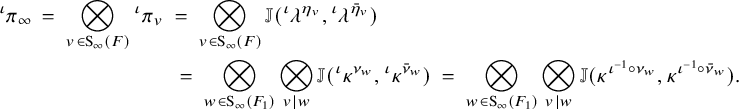(2.17) $$ \begin{align} {}^\iota\pi_\infty \ = \ \bigotimes_{v \in \mathrm{S}_\infty(F)} {}^\iota\pi_v \ &= \ \bigotimes_{v \in \mathrm{S}_\infty(F)} \mathbb{J}({}^\iota\lambda^{\eta_{v}}, {}^\iota\lambda^{\bar{\eta}_{v}}) \notag\\ & \ = \ \bigotimes_{w \in \mathrm{S}_\infty(F_1)} \bigotimes_{v|w} \mathbb{J}({}^\iota\kappa^{\nu_{w}}, {}^\iota\kappa^{\bar\nu_{w}}) \ = \ \bigotimes_{w \in \mathrm{S}_\infty(F_1)} \bigotimes_{v|w} \mathbb{J}(\kappa^{\iota^{-1} \circ \nu_{w}}, \kappa^{\iota^{-1} \circ \bar\nu_{w}}). \end{align} $$

TR-case

We still have from Proposition 2.6 that $\lambda = \mathrm {BC}_{F/F_1}(\kappa );$ that is, $\lambda ^\tau = \kappa ^{\tau |_{F_1}};$ after applying $\iota $ , one has ${}^\iota \lambda ^\eta = {}^\iota \kappa ^{\eta |_{F_1}},$ which is the same as $\lambda ^{\iota ^{-1}\circ \eta } = \kappa ^{\iota ^{-1}\circ \eta |_{F_1}}.$ Using the notations fixed in 2.3.5, for any place $v_{jl} \in \mathrm {S}_\infty (F)$ above $w_j \in \mathrm {S}_\infty (F_1),$ both the embeddings in the ordered pair $(\eta _{v_{jl}}, \bar {\eta }_{v_{jl}})$ restrict to $\nu _{w_j}$ . Hence, the ordered pair of weights $({}^\iota \lambda ^{\eta _{v_{jl}}}, {}^\iota \lambda ^{\bar {\eta }_{v_{jl}}})$ is equal to the ordered pair $({}^\iota \kappa ^{\nu _{w_j}}, {}^\iota \kappa ^{\nu _{w_j}})$ – note that both weights in the ordered pair are the same, whence the archimedean component ${}^\iota \pi _{v_{jl}}$ is equivalent to $\mathbb {J}({}^\iota \kappa ^{\nu _{w_j}}, {}^\iota \kappa ^{\nu _{w_j}})$ . Once again, for brevity, denoting $\mathbb {J}({}^\iota \kappa ^{\nu _{w_j}}, {}^\iota \kappa ^{\nu _{w_j}})$ by $\mathbb {J}_{w_j}$ , one concludes that the constituents of ${}^\iota \pi _\infty $ are elements of the multi-set $\{\mathbb {J}_{w_1},\dots , \mathbb {J}_{w_1}, \ \dots \ ,\mathbb {J}_{w_{{\mathrm r}_1}}, \dots , \mathbb {J}_{w_{{\mathrm r}_1}} \},$ with each $\mathbb {J}_{w_j}$ appearing $k_1 = [F:F_1]/2$ -many times; putting these together, one has

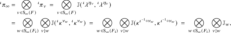(2.18) $$ \begin{align} {}^\iota\pi_\infty &= \bigotimes_{v \in \mathrm{S}_\infty(F)} {}^\iota\pi_v \ = \ \bigotimes_{v \in \mathrm{S}_\infty(F)} \mathbb{J}({}^\iota\lambda^{\eta_{v}}, {}^\iota\lambda^{\eta_{v}})\notag\\& = \bigotimes_{w \in \mathrm{S}_\infty(F_1)} \bigotimes_{v|w} \mathbb{J}({}^\iota\kappa^{\nu_{w}}, {}^\iota\kappa^{\nu_{w}}) \ = \ \bigotimes_{w \in \mathrm{S}_\infty(F_1)} \bigotimes_{v|w} \mathbb{J}(\kappa^{\iota^{-1} \circ \nu_{w}}, \kappa^{\iota^{-1} \circ \nu_{w}}) \ = \ \bigotimes_{w \in \mathrm{S}_\infty(F_1)} \bigotimes_{v|w} \mathbb{J}_w, \end{align} $$

and each of these $\mathbb {J}_w$ is self-conjugate from Remark 2.12.

2.5.3 Galois action on archimedean constituents

Let $\gamma \in \mathrm {{Gal}}(\bar {\mathbb {Q}}/\mathbb {Q}).$ The archimedean constituents of ${}^{\gamma \circ \iota }\pi $ is a permutation of the archimedean constituents of ${}^\iota \pi $ , possibly up to replacing a local component by its conjugate which will only be relevant when F is in the CM-case. This is made more precise in the following paragraphs.

The case when F is itself a CM field

If $F = F_1$ is a CM field, and $F_0$ its maximal totally real quadratic subfield, for $\gamma \in \mathrm {{Gal}}(\bar {\mathbb {Q}}/\mathbb {Q})$ and $\nu \in \Sigma _{F_1}$ from Lemma 2.5, one has $\gamma \circ \bar {\nu } = \overline { \gamma \circ \nu };$ this means that $\gamma $ permutes the set of pairs of conjugate embeddings $\left \{\{\nu _w, \bar \nu _w\} \ | \ w \in \mathrm {S}_\infty (F_1)\right \}$ , giving an action of $\gamma $ on $\mathrm {S}_\infty (F_1)$ . If we identify $\mathrm {S}_\infty (F_1) = \mathrm {S}_\infty (F_0) = \Sigma _{F_0}$ , then the action of $\gamma $ on $\mathrm {S}_\infty (F_1)$ is the same as action of $\gamma $ on $\Sigma _{F_0}$ via composition. It is important to note that $\gamma $ need not map the distinguished embedding corresponding to w to the distinguished embedding corresponding to $\gamma \cdot w$ ; all one can say is that $\gamma \circ \nu _w \in \{\nu _{\gamma \cdot w}, \bar {\nu }_{\gamma \cdot w}\}.$ Suppose $\kappa \in X^+_{00}(\mathrm {Res}_{F_1/\mathbb {Q}}(T_{N,0}) \times E)$ , $\pi _{1,f} \in \mathrm {{Coh}}_{!!}(\mathrm {Res}_{F_1/\mathbb {Q}}(\mathrm {{GL}}_N/F_1,\kappa ))$ , $\iota : E \to \mathbb {C}$ , and ${}^\iota \pi _1$ the corresponding cuspidal automorphic representation of $\mathrm {{GL}}_N(\mathbb {A}_{F_1})$ . Then ${}^\iota \pi _{1,\infty } = \otimes _{w \in \mathrm {S}_\infty (F_1)} {}^\iota \pi _{1,w}$ , where

$$ \begin{align*}{}^\iota\pi_{1,w} \ = \ \mathbb{J}({}^\iota\kappa^{\nu_w}, {}^\iota\kappa^{\bar\nu_w}) \ = \ \mathbb{J}(\kappa^{\iota^{-1} \circ \nu_w}, \kappa^{\iota^{-1} \circ \bar\nu_w}). \end{align*} $$

By the same token, replacing $\iota $ by $\gamma \circ \iota $ , one has

$$ \begin{align*}{}^{\gamma \circ \iota} \pi_{1,w} \ = \ \mathbb{J}(\kappa^{\iota^{-1} \circ \gamma^{-1} \circ \nu_w}, \kappa^{\iota^{-1} \circ \gamma^{-1} \circ \bar\nu_w}) \ = \ \mathbb{J}(\kappa^{\iota^{-1} \circ \gamma^{-1} \circ \nu_w}, \kappa^{\iota^{-1} \circ \overline{\gamma^{-1} \circ \nu_w}}) \end{align*} $$

Depending on whether $\gamma ^{-1} \circ \nu _w = \nu _{\gamma ^{-1} \cdot w}$ or $\overline {\nu _{\gamma ^{-1} \cdot w}}$ , from Remark 2.12, it follows that

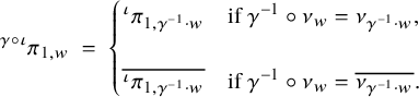(2.19) $$ \begin{align} {}^{\gamma \circ \iota} \pi_{1,w} \ = \ \begin{cases} {}^\iota\pi_{1, \gamma^{-1} \cdot w} & \mbox{if } \gamma^{-1} \circ \nu_w = \nu_{\gamma^{-1} \cdot w}, \\ \\ \overline{{}^\iota\pi_{1, \gamma^{-1} \cdot w}} & \mbox{if } \gamma^{-1} \circ \nu_w = \overline{\nu_{\gamma^{-1} \cdot w}}. \end{cases} \end{align} $$

Hence, the archimedean components of ${}^{\gamma \circ \iota } \pi _1$ is a permutation of the archimedean components of ${}^{\iota } \pi _1$ up to taking conjugates; this paragraph fixes a mistake in [12, Prop. 3.2, (i)].

When F is totally imaginary in the CM-case.

Let $\lambda \in X^+_{00}(\mathrm {Res}_{F/\mathbb {Q}}(T_{N,0}) \times E)$ , $\lambda = \mathrm { BC}_{F/F_1}(\kappa )$ , $\pi _f \in \mathrm {{Coh}}_{!!}(G,\lambda )$ , $\iota : E \to \mathbb {C}$ , and $\gamma \in \mathrm {{Gal}}(\bar {\mathbb {Q}}/\mathbb {Q})$ . The Galois action on $\Sigma _F$ and $\Sigma _{F_1}$ preserves the fibers of the restriction map $\Sigma _F \to \Sigma _{F_1}$ . Suppose $w_1, w_j \in \mathrm {S}_\infty (F_1)$ and $\nu _1, \nu _j \in \Sigma _{F_1}$ are the corresponding distinguished elements, and suppose $\gamma \circ \{\nu _1, \bar \nu _1\} = \{\nu _j, \bar \nu _j\}$ . Suppose the fiber over $\nu _1$ is $\{\eta _{11}, \eta _{12}, \dots , \eta _{1 k}\}$ (recall $k = [F:F_1]$ ). Then the fiber over $\bar \nu _1$ is $\{\bar {\eta }_{11}, \bar {\eta }_{12}, \dots , \bar {\eta }_{1 k}\}$ ; and similarly, if the fiber over $\nu _j$ is $\{\eta _{j1}, \eta _{j2}, \dots , \eta _{j k}\}$ and then the fiber over $\bar \nu _j$ is $\{\bar {\eta }_{j1}, \bar {\eta }_{j2}, \dots , \bar {\eta }_{j k}\}.$ There are two cases:

1. 1. $\gamma \circ \nu _1 = \nu _j$ . Then necessarily, $\gamma \circ \bar \nu _1 = \bar \nu _j$ , $\gamma \circ \{\eta _{11}, \dots , \eta _{1 k}\} = \{\eta _{j1}, \dots , \eta _{j k}\}$ and $\gamma \circ \{\bar {\eta }_{11}, \dots , \bar {\eta }_{1 k}\} = \{\bar {\eta }_{j1}, \dots , \bar {\eta }_{j k}\}.$

2. 2. $\gamma \circ \nu _1 = \bar \nu _j$ . Then necessarily, $\gamma \circ \bar \nu _1 = \nu _j$ , $\gamma \circ \{\eta _{11}, \dots , \eta _{1 k}\} = \{\bar {\eta }_{j1}, \dots , \bar {\eta }_{j k}\} $ and $\gamma \circ \{\bar {\eta }_{11}, \dots , \bar {\eta }_{1 k}\} = \{\eta _{j1}, \dots , \eta _{j k}\}.$

Since $F = F_1$ is already discussed in 2.5.3 above, suppose that $k> 1$ . Suppose $\gamma \circ \eta _{11} = \eta _{j1}$ . Then it is possible that $\gamma \circ \{\eta _{11}, \bar {\eta }_{11}\} \neq \{\eta _{j1}, \bar {\eta }_{j1}\}.$ In particular, the Galois action on $\Sigma _F$ does not descend to give a Galois action of $\gamma $ on $S_\infty (F)$ . Similarly, also in case (2). Nevertheless, using (2.17), it follows that

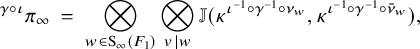(2.20) $$ \begin{align} {}^{\gamma\circ\iota}\pi_\infty \ = \ \bigotimes_{w \in \mathrm{S}_\infty(F_1)} \bigotimes_{v|w} \mathbb{J}(\kappa^{\iota^{-1} \circ \gamma^{-1} \circ \nu_{w}}, \kappa^{\iota^{-1} \circ \gamma^{-1} \circ \bar\nu_{w}}), \end{align} $$

and as in (2.19), the inner constituent is given by

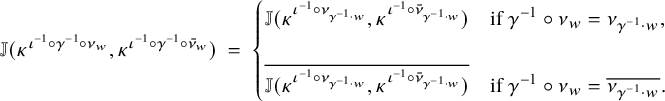(2.21) $$ \begin{align} \mathbb{J}(\kappa^{\iota^{-1} \circ \gamma^{-1} \circ \nu_{w}}, \kappa^{\iota^{-1} \circ \gamma^{-1} \circ \bar\nu_{w}}) \ = \ \begin{cases} \mathbb{J}(\kappa^{\iota^{-1} \circ \nu_{\gamma^{-1} \cdot w}}, \kappa^{\iota^{-1} \circ \bar\nu_{\gamma^{-1} \cdot w}}) & \mbox{if } \gamma^{-1} \circ \nu_w = \nu_{\gamma^{-1} \cdot w}, \\ \\ \overline{ \mathbb{J}(\kappa^{\iota^{-1} \circ \nu_{\gamma^{-1} \cdot w}}, \kappa^{\iota^{-1} \circ \bar\nu_{\gamma^{-1} \cdot w}})} & \mbox{if } \gamma^{-1} \circ \nu_w = \overline{\nu_{\gamma^{-1} \cdot w}}. \end{cases} \end{align} $$

Hence, the archimedean components of ${}^{\gamma \circ \iota } \pi $ is a permutation of the archimedean components of ${}^{\iota } \pi $ up to taking conjugates.

When F is totally imaginary in the TR-case.

The Galois action on $\Sigma _F$ and $\Sigma _{F_1}$ preserves the fibers of the restriction map $\Sigma _F \to \Sigma _{F_1}$ , and since $F_1$ is totally real, identify the Galois-sets $\Sigma _{F_1} = \mathrm {S}_\infty (F_1).$ Using the notations of (2.18), if

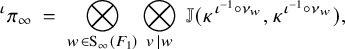$$ \begin{align*} {}^\iota\pi_\infty \ = \ \bigotimes_{w \in \mathrm{S}_\infty(F_1)} \bigotimes_{v|w} \ \mathbb{J}(\kappa^{\iota^{-1} \circ \nu_{w}}, \kappa^{\iota^{-1} \circ \nu_{w}}), \end{align*} $$

then for $\gamma \in \mathrm {{Gal}}(\bar {\mathbb {Q}}/\mathbb {Q})$ , one has

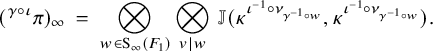$$ \begin{align*} ({}^{\gamma \circ \iota} \pi)_\infty \ = \ \bigotimes_{w \in \mathrm{S}_\infty(F_1)} \bigotimes_{v|w} \ \mathbb{J}(\kappa^{\iota^{-1} \circ \nu_{\gamma^{-1}\circ w}}, \kappa^{\iota^{-1} \circ \nu_{\gamma^{-1}\circ w}}). \end{align*} $$

Hence, the archimedean components of ${}^{\gamma \circ \iota } \pi $ is a permutation of the archimedean components of ${}^{\iota } \pi $ .

2.6 Boundary cohomology

The cohomology $H^{\bullet }(\partial \mathcal {S}^G_{K_f}, \widetilde {\mathcal {M}}_{\lambda ,E})$ of the boundary of the Borel–Serre compactification of the locally symmetric space $\mathcal {S}^G_{K_f}$ is briefly discussed here, and the reader is referred to [27, Chap. 4] for more details and proofs. There is a spectral sequence built from the cohomology of the boundary strata $ \partial _P\mathcal {S}^G_{K_f}$ that converges to the cohomology of the boundary. To understand the cohomology of a single stratum $\partial _P\mathcal {S}^G_{K_f},$ note that

$$ \begin{align*}H^{\bullet}(\partial_P\mathcal{S}^G_{K_f}, \widetilde{\mathcal{M}}_{\lambda,E}) \ = \ H^{\bullet}(P(\mathbb{Q})\backslash G(\mathbb{A})/ K_\infty K_f, \widetilde{\mathcal{M}}_{\lambda,E}). \end{align*} $$

The space $P(\mathbb {Q})\backslash G(\mathbb {A})/ K_\infty K_f$ fibers over locally symmetric spaces of $M_P.$ Let $\Xi _{K_f}$ be a complete set of representatives for $P(\mathbb {A}_f)\backslash G(\mathbb {A}_f)/K_f.$ Let $K^P_\infty = K_\infty \cap P(\mathbb {R}),$ and for $\xi _f \in \Xi _{K_f}$ , let $K_f^P(\xi _f) = P(\mathbb {A}_f) \cap \xi _f K_f \xi _f^{-1}.$ Then

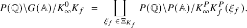$$ \begin{align*}P(\mathbb{Q})\backslash G(\mathbb{A})/ K_\infty^0K_f \ = \ \coprod_{\xi_f \, \in \, \Xi_{K_f}} P(\mathbb{Q})\backslash P(\mathbb{A})/ K^P_\infty K_f^P(\xi_f). \end{align*} $$

Let $\kappa _P : P \to P/U_P = M_P$ be the canonical map, and define $K_\infty ^{M_P} = \kappa _P(K^P_\infty )$ , and for $\xi _f \in \Xi _{K_f}$ , let $K_f^{M_P}(\xi _f) = \kappa _P(K_f^P(\xi _f)).$ Define

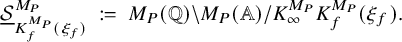$$ \begin{align*}\underline{\mathcal{S}}^{M_P}_{K_f^{M_P}(\xi_f)} \ := \ M_P(\mathbb{Q})\backslash M_P(\mathbb{A}) / K_\infty^{M_P}K_f^{M_P}(\xi_f). \end{align*} $$

The underline is to emphasize that we have divided by $K_\infty ^{M_P}$ that may be explicated as follows: for the maximal parabolic $P = P_{(n,n')},$ whose Levi quotient $M_P$ may be identified with the block diagonal subgroup $G_n \times G_{n'}$ where $G_n = R_{F/\mathbb {Q}}(\mathrm {{GL}}_n)$ and $G_{n'} = R_{F/\mathbb {Q}}(\mathrm {{GL}}_{n'}),$ one has

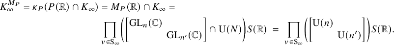$$ \begin{align*} K_\infty^{M_P} = \kappa_P(P(\mathbb{R}) \cap K_\infty) &= M_P(\mathbb{R}) \cap K_\infty = \\ &\prod_{v \in \mathrm{S}_\infty} \left(\begin{bmatrix} \mathrm{{GL}}_n(\mathbb{C}) & \\ & \mathrm{{GL}}_{n'}(\mathbb{C}) \end{bmatrix} \cap \mathrm{{U}}(N) \right) S(\mathbb{R}) \ = \ \prod_{v \in \mathrm{S}_\infty} \left(\begin{bmatrix} \mathrm{{U}}(n) & \\ & \mathrm{{U}}(n') \end{bmatrix} \right) S(\mathbb{R}). \end{align*} $$

Note that $K_\infty ^{M_P}$ is connected. Let $K_f^{U_P}(\xi _f) = U_P(\mathbb {A}_f) \cap \xi _f K_f \xi _f^{-1}.$ We have the fibration

$$ \begin{align*}U_P(\mathbb{Q})\backslash U_P(\mathbb{A})/K_f^{U_P}(\xi_f) \ \hookrightarrow \ P(\mathbb{Q})\backslash P(\mathbb{A})/ K^P_\infty K_f^P(\xi_f) \ \twoheadrightarrow \ \underline{\mathcal{S}}^{M_P}_{K_f^{M_P}(\xi_f)}. \end{align*} $$

The corresponding Leray–Serre spectral sequence is known to degenerate at the $E_2$ -level. The cohomology of the total space is given in terms of the cohomology of the base with coefficients in the cohomology of the fiber. For the cohomology of the fiber, if ${\mathfrak {u}}_P$ is the Lie algebra of $U_P$ , then the cohomology of the fiber is the same as the Lie algebra cohomology group $H^{\bullet }({\mathfrak {u}}_P, \mathcal {M}_{\lambda , E})$ –by a classical theorem due to van Est, which is naturally an algebraic representation of $M_P$ ; the associated sheaf on $\underline {\mathcal {S}}^{M_P}_{K_f^{M_P}(\xi _f)}$ is denoted by putting a tilde on top. One has

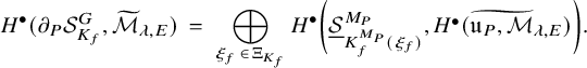(2.22) $$ \begin{align} H^{\bullet}(\partial_P\mathcal{S}^G_{K_f}, \widetilde{\mathcal{M}}_{\lambda,E}) \ = \ \bigoplus_{\xi_f \, \in \, \Xi_{K_f}} H^{\bullet} \left(\underline{\mathcal{S}}^{M_P}_{K_f^{M_P}(\xi_f)}, \widetilde{H^{\bullet}({\mathfrak{u}}_P, \mathcal{M}_{\lambda,E})}\right). \end{align} $$

Pass to the limit over all open compact subgroups $K_f$ and define $H^{\bullet }(\partial _P\mathcal {S}^G, \widetilde {\mathcal {M}}_{\lambda ,E}) := \varinjlim _{K_f} H^{\bullet }(\partial _P\mathcal {S}^G_{K_f}, \widetilde {\mathcal {M}}_{\lambda ,E}). $ Let $\underline {\mathcal {S}}^{M_P} \ := \ M_P(\mathbb {Q})\backslash M_P(\mathbb {A}) / K_\infty ^{M_P};$ (2.22) can be rewritten as

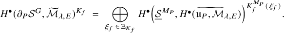$$ \begin{align*}H^{\bullet}(\partial_P\mathcal{S}^G, \widetilde{\mathcal{M}}_{\lambda,E})^{K_f} \ = \ \bigoplus_{\xi_f \, \in \, \Xi_{K_f}} H^{\bullet} \left(\underline{\mathcal{S}}^{M_P}, \widetilde{H^{\bullet}({\mathfrak{u}}_P, \mathcal{M}_{\lambda,E})}\right)^{K_f^{M_P}(\xi_f)}. \end{align*} $$

It is clear using Mackey theory that the right-hand side is the $K_f$ -invariants of an algebraically induced representation; hence, one has the following:

Proposition 2.23. The cohomology of $\partial _P\mathcal {S}^G$ is given by

$$ \begin{align*}H^{\bullet}(\partial_P\mathcal{S}^G, \widetilde{\mathcal{M}}_{\lambda,E}) \ = \ {{}^{\mathrm{a}}\mathrm{Ind}}_{P(\mathbb{A}_f)}^{G(\mathbb{A}_f)} \left( H^{\bullet}(\underline{\mathcal{S}}^{M_P}, \widetilde{H^{\bullet}({\mathfrak{u}}_P, \mathcal{M}_{\lambda,E})}) \right). \end{align*} $$

The notation ${{}^{\mathrm {a}}\mathrm {Ind}}$ stands for algebraic, or un-normalized, induction.

The following is a brief review of well-known results of Kostant [36] on the structure of $H^{\bullet }({\mathfrak {u}}_P, \mathcal {M}_{\lambda , E}).$ The calculation of the unipotent cohomology group is over the field E. Recall that $G \times E = \prod _{\tau : F \to E} G_0^\tau $ , where $G_0^\tau = G_0 \times _{F,\tau } E = \mathrm {{GL}}_N/E.$ Let $\mathbf {\Delta }_{G_0}$ stand for the set of roots of $G_0$ with respect to $T_{N,0}$ , $\mathbf {\Delta }_{G_0}^+$ the subset of positive roots (for choice of Borel subgroup being the upper triangular subgroup), and $\mathbf {\Pi }_{G_0}$ the set of simple roots. The notations $\mathbf {\Delta }_{G_0^\tau }$ , $\mathbf {\Delta }_{G_0^\tau }^+$ and $\mathbf {\Pi }_{G_0^\tau }$ are clear. Let $P = \mathrm {Res}_{F/\mathbb {Q}}(P_0)$ be the parabolic subgroup of G as above, and let $P_0^\tau := P_0 \times _{\tau } E.$ The Weyl group factors as $W = \prod _{\tau : F \to E} W_0^\tau $ with each $W_0^\tau $ isomorphic to the permutation group $\mathfrak {S}_N$ on N-letters. Let $W^P$ be the set of Kostant representatives in the Weyl group W of G corresponding to the parabolic subgroup P defined as $W^P = \{ w = (w^\tau ) : w^\tau \in W^\tau _0{}^{P^\tau _0} \},$ where

$$ \begin{align*}W^\tau_0{}^{P^\tau_0} \ := \{w^\tau \in W^\tau_0 : \ (w^\tau)^{-1}\alpha> 0, \ \forall \alpha \in \mathbf{\Pi}_{M_{P_0^\tau}} \}. \end{align*} $$

Here, $\mathbf {\Pi }_{M_{P_0^\tau }} \subset \mathbf {\Pi }_{G_0^\tau }$ denotes the set of simple roots in the Levi quotient $M_{P_0^\tau }$ of $P_0^\tau .$ The twisted action of $w \in W$ on $\lambda \in X^{*}(T)$ is $w \cdot \lambda = (w^\tau \cdot \lambda ^\tau )_{\tau : F \to E}$ and where For $w \in W^P$ , the irreducible finite-dimensional representation of $M_P \times E$ with extremal weight $w \cdot \lambda $ is denoted $\mathcal {M}_{w\cdot \lambda , E}$ . Kostant’s theorem asserts that one has a multiplicity-free decomposition of $M_P \times E$ -modules:

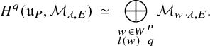(2.24) $$ \begin{align} H^q({\mathfrak{u}}_P, \mathcal{M}_{\lambda, E}) \ \simeq \ \bigoplus_{\substack{w \in W^P \\ l(w) = q}} \mathcal{M}_{w \cdot \lambda, E}. \end{align} $$

As explained in [27], the above result of Kostant can be parsed over the set of embeddings ${\tau : F \to E.}$ Denote by $H^{l(w)}({\mathfrak {u}}_P, \mathcal {M}_{\lambda , E})(w)$ the summand of $H^q({\mathfrak {u}}_P, \mathcal {M}_{\lambda , E})$ corresponding to the Kostant representative w which is nonzero for $q = l(w)$ and isomorphic to $\mathcal {M}_{w \cdot \lambda , E}$ . Applying (2.24) to the boundary cohomology as in Proposition 2.23 gives the following:

Proposition 2.25. The cohomology of $\partial _P\mathcal {S}^G$ is given by

$$ \begin{align*}H^q(\partial_P\mathcal{S}^G, \widetilde{\mathcal{M}}_{\lambda, E}) \ = \ \bigoplus_{w \in W^P} {}^{\mathrm{a}}\mathrm{Ind}_{P(\mathbb{A}_f)}^{G(\mathbb{A}_f)} \left(H^{q - l(w)}(\underline{\mathcal{S}}^{M_P}, \widetilde{H^q({\mathfrak{u}}_P, \mathcal{M}_{\lambda, E})(w)} ) \right). \end{align*} $$

There is a canonical surjection $\underline {\mathcal {S}}^{M_P} \to \mathcal {S}^{M_P}$ , using which we may inflate up the cohomology of $\mathcal {S}^{M_P}$ to the cohomology of $\underline {\mathcal {S}}^{M_P}$ ; this will be especially relevant to strongly inner cohomology classes of $\mathcal {S}^{M_P}$ , which after inducing up to $G(\mathbb {A}_f)$ will contribute to boundary cohomology; see Section 5.1.2.

2.7 Galois action and local systems in boundary cohomology

For an embedding $\iota : E \to \mathbb {C}$ , the map $\gamma _*$ induced by a Galois element $\gamma \in \mathrm {{Gal}}(\bar {\mathbb {Q}}/\mathbb {Q})$ in unipotent cohomology

$$ \begin{align*}H^q({\mathfrak{u}}_P, \mathcal{M}_{{}^\iota\!\lambda, \mathbb{C}})({}^\iota w) \ \to \ H^q({\mathfrak{u}}_P, \mathcal{M}_{{}^{\gamma \circ \iota} \! \lambda, \mathbb{C}})({}^{\gamma \circ \iota} w), \end{align*} $$

where, $q = l(w) = l({}^\iota w) = l({}^{\gamma \circ \iota } w)$ , will play a role in the proof of the reciprocity law of the main theorem. By Schur’s lemma, this can be understood by its effect on the highest weight vector for the irreducible representation $H^q({\mathfrak {u}}_P, \mathcal {M}_{{}^\iota \!\lambda , \mathbb {C}})({}^\iota w) \simeq \mathcal {M}_{{}^\iota w \cdot {}^\iota \!\lambda , \mathbb {C}}.$ Such a highest weight vector ${\mathrm h}(\lambda , w, \iota )$ will be fixed by fixing a harmonic representative the corresponding cohomology class as in Kostant [36, Thm. 5.14]. To explicate this vector, note that

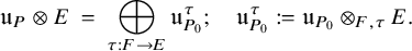$$ \begin{align*}{\mathfrak{u}}_P \otimes E \ = \ \bigoplus_{\tau : F \to E} {\mathfrak{u}}_{P_0}^\tau; \quad {\mathfrak{u}}_{P_0}^\tau := {\mathfrak{u}}_{P_0} \otimes_{F, \tau} E. \end{align*} $$

Fix an ordering

$$ \begin{align*}\mathrm{{Hom}}(F, E) = \{\tau_1,\tau_2,\dots,\tau_d\}. \end{align*} $$

Let $\mathbf {\Delta }({\mathfrak {u}}_{P_0})$ denote the subset of $\mathbf {\Delta }^+$ of those positive roots $\varphi $ whose root space $X_\varphi $ is in ${\mathfrak {u}}_{P_0}$ . Fix an ordering

$$ \begin{align*}\mathbf{\Delta}({\mathfrak{u}}_{P_0}) = \{\varphi_1,\varphi_2,\dots,\varphi_{nn'}\}. \end{align*} $$

For example, thinking in terms of upper triangular matrices, this ordering could be taken as the lexicographic ordering on the set of pairs of indices $\{(i,j): 1 \leq i \leq n, \ 1 \leq j \leq n'\}$ . Fix a generator $e_\varphi $ for $X_\varphi $ for each $\varphi \in \mathbf {\Delta }({\mathfrak {u}}_{P_0});$ note that $e_\varphi $ is well defined up to $\mathbb {Q}^{\times }.$ Let $\{e_\varphi ^{*}\}$ denote the basis of ${\mathfrak {u}}_{P_0}^{*}$ that is dual to $\{e_\varphi \}.$ For a Kostant representative $w_0 \in W^{P_0} \subset W_{G_0}$ , define $\Phi _{w_0} = \{\varphi> 0 : w_0^{-1}\varphi < 0\};$ then $\Phi _{w_0} \subset \mathbf {\Delta }({\mathfrak {u}}_{P_0})$ . With respect to the ordering that it inherits from $\mathbf {\Delta }({\mathfrak {u}}_{P_0})$ , denote $\Phi _{w_0} = \{\varphi ^{w_0}_1, \dots ,\varphi ^{w_0}_{l}\}$ as an ordered set, where $l = l(w_0^{-1}) = l(w_0).$ Define

$$ \begin{align*}e_{\Phi_{w_0}}^{*} \ := \ e_{\varphi^{w_0}_1}^{*} \wedge \cdots \wedge e_{\varphi^{w_0}_l}^{*} \ \in \ \wedge^{q_0}({\mathfrak{u}}_{P_0}^{*}); \quad q_0 := l(w_0). \end{align*} $$

Let $e_\varphi ^\tau $ denote the image $e_\varphi \otimes 1$ of $e_\varphi $ under the canonical map $X_\varphi \to X_\varphi ^\tau = X_\varphi \otimes _{F,\tau } E$ . For $w = (w^\tau )_{\tau : F \to E} \in W_G = \prod _{\tau : F \to E} W_{G_0} \times _{F, \tau } E$ , written using the ordering on $\mathrm {{Hom}}(F, E)$ as $w = \{w^{\tau _1}, \dots , w^{\tau _d}\}$ , define

$$ \begin{align*}e_{\Phi_w}^{*} \ := \ e_{\Phi_{w^{\tau_1}}}^{*} \wedge \cdots \wedge e_{\Phi_{w^{\tau_d}}}^{*} \ \in \ \wedge^q({\mathfrak{u}}_{P}^{*}\otimes E); \quad q := l(w). \end{align*} $$

Changing the base to $\mathbb {C}$ via $\iota : E \to \mathbb {C}$ gives

(2.26) $$ \begin{align} e_{\Phi_{^\iota \! w}}^{*} \ := \ e_{\Phi_{w^{\iota \circ \tau_1}}}^{*} \wedge \cdots \wedge e_{\Phi_{w^{\iota \circ \tau_d}}}^{*} \ \in \ \wedge^q({\mathfrak{u}}_{P}^{*} \otimes_{\mathbb{Q}} \mathbb{C}). \end{align} $$

Fix a weight vector ${\mathrm s}(\lambda ^\tau ) \in \mathcal {M}_{\lambda ^\tau , E}$ for the highest weight $\lambda ^\tau ;$ then ${\mathrm s}(\lambda ) = {\mathrm s}(\lambda ^\tau _1) \otimes \cdots \otimes {\mathrm s}(\lambda ^\tau _d)$ is the highest weight vector for $\mathcal {M}_{\lambda , E}$ . For each $w \in W,$ fix its representative in $G(E)$ , which amounts to fixing a permutation matrix representing $w^\tau $ in $\mathrm {{GL}}_n(E)$ for each embedding $\tau : F \to E$ . Let

(2.27) $$ \begin{align} {\mathrm s}(w \lambda) \ := \ \rho_{\lambda^{\tau_1}}(w^{\tau_1}){\mathrm s}(\lambda^\tau_1) \otimes \cdots \otimes \rho_{\lambda^{\tau_d}}(w^{\tau_d}){\mathrm s}(\lambda^\tau_d) \end{align} $$

be the weight vector of extremal weight $w\lambda .$ These vectors can be composed via $\iota $ : ${\mathrm s}({}^\iota \!w \, {}^\iota \!\lambda )$ is the weight vector in $\mathcal {M}_{{}^\iota \!\lambda , \mathbb {C}}$ of extremal weight ${}^\iota \!w \, {}^\iota \!\lambda .$ Theorem 5.14 of [36] asserts that

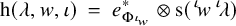(2.28) $$ \begin{align} {\mathrm h}(\lambda, w, \iota) \ = \ e_{\Phi_{^\iota \! w}}^{*} \otimes {\mathrm s}({}^\iota \!w \, {}^\iota\!\lambda) \end{align} $$

is the highest weight vector for $H^q({\mathfrak {u}}_P, \mathcal {M}_{{}^\iota \!\lambda , \mathbb {C}})({}^\iota w).$ The image of ${\mathrm h}(\lambda , w, \iota )$ under the map $\gamma _*$ induced by $\gamma \in \mathrm {{Gal}}(\bar {\mathbb {Q}}/\mathbb {Q})$ is a multiple of ${\mathrm h}(\lambda , w, \gamma \circ \iota )$ ; the scaling factor is captured by what $\gamma $ does to the wedge-products $e_{\Phi _{^\iota \! w}}^{*}$ , motivating the following:

Definition 2.29. Let $\iota : E \to \mathbb {C}$ and $\gamma \in \mathrm {{Gal}}(\bar {\mathbb {Q}}/\mathbb {Q})$ . Then we have

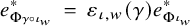$$ \begin{align*}e_{\Phi_{^{\gamma \circ \iota} \! w}}^{*} \ = \ \varepsilon_{\iota, w}(\gamma) e_{\Phi_{^\iota \! w}}^{*} \end{align*} $$

for a signature $\varepsilon _{\iota , w}(\gamma ) \in \{\pm 1\}$ .

From (2.27), (2.28), and the above definition, one has

(2.30) $$ \begin{align} \gamma_*({\mathrm h}(\lambda, w, \iota)) \ = \ \varepsilon_{\iota, w}(\gamma) \cdot {\mathrm h}(\lambda, w, \gamma \circ \iota). \end{align} $$

3 The critical set and a combinatorial lemma

In Section 3.1, we first recall the definition of an integer or possibly a half-integer being critical for the Rankin–Selberg L-function $L(s, \sigma \times \sigma ^{\prime \mathrm {v}})$ ; see (3.4). Then in Proposition 3.12, we describe the set of critical points in terms of the highest weights $\mu $ and $\mu '$ , from which we get a purely combinatorial characterization of when the point of evaluation $-N/2$ and the next point $1-N/2$ are critical; see Corollary 3.13. In Section 3.2, we begin by stating the combinatorial lemma (Lemma 3.16) which builds on Corollary 3.13 and characterizes criticality of $-N/2$ and $1-N/2$ also in terms of the existence of a balanced Kostant representative w whose twisted action on $\mu + \mu '$ yields a dominant integral weight on the ambient $\mathrm {{GL}}_N/F$ . The rest of the subsection goes in proving this lemma. This special Weyl group element w plays an important role in all that follows. For a first reading, we recommend the reader to assume the statement of Lemma 3.16 and come back to its proof at a later point of time.

3.1 The critical set for $L(s, \sigma \times \sigma ^{\prime \mathrm {v}})$

Let n and $n'$ be two positive integers, and consider weights $\mu \in X^+_{00}(T_n \times \mathbb {C})$ and $\mu ' \in X^+_{00}(T_{n'} \times \mathbb {C})$ given by

(3.1)

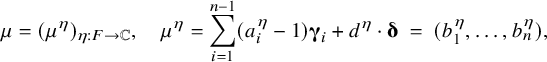
and similarly,

(3.2)

Let $\sigma _f \in \mathrm {{Coh}}_{!!}(G_n, \mu )$ and $\sigma ^{\prime }_f \in \mathrm {{Coh}}_{!!}(G_{n'}, \mu ')$ be strongly inner Hecke-summands; these Hecke-summands take a unique representation at infinity to contribute to the respective cuspidal spectrum cohomology. Denote $\sigma _\infty = \mathbb {J}_\mu $ and $\sigma ^{\prime }_\infty = \mathbb {J}_{\mu '}$ . Then $\sigma = \sigma _\infty \otimes \sigma _f$ and $\sigma ' = \sigma ^{\prime }_\infty \otimes \sigma ^{\prime }_f$ are cuspidal automorphic representations. We let $L(s, \sigma \times \sigma ')$ stand for the completed standard Rankin–Selberg L-function of degree $nn'.$ We refer the reader to [47, Sect. 10.1] for a summary of the basic analytic properties of these L-functions. The purpose of this section is to identify the set of integers or possibly half-integers m which are critical for $L(s, \sigma \times \sigma ^{\prime \mathrm {v}}).$ (Note that we have dualized $\sigma '.$ )

3.1.1 Definition of the critical set

For any two half-integers $\alpha $ and $\beta ,$ the local L-factor (see [35]) of the character $z \mapsto z^\alpha \bar {z}^\beta $ of $\mathbb {C}^{\times }$ is given by

(3.3) $$ \begin{align} L(s, z^\alpha \bar{z}^\beta) = 2(2\pi)^{-\left(s + \frac{\alpha+\beta}{2} + \frac{|\alpha - \beta|}{2}\right)} \Gamma\left(s + \frac{\alpha+\beta}{2} + \frac{|\alpha - \beta|}{2}\right) \sim \Gamma\left(s + \frac{\alpha+\beta}{2} + \frac{|\alpha - \beta|}{2}\right), \end{align} $$

where, by $\sim $ , we mean up to nonzero constants and exponential functions, which are entire and nonvanishing everywhere and hence are irrelevant to the computation of critical points; see Definition 3.4 below. For any $v \in \mathrm {S}_\infty $ , let $\{\eta _v, \bar {\eta }_v\}$ be the pair of conjugate embeddings of F to $\mathbb {C}$ as before. Let

be the cuspidal parameters of $\mu $ at v; see (2.8) and (2.9). Similarly, let

be the cuspidal parameters of $\mu '$ at $v.$ Note that

$$ \begin{align*}\alpha := \alpha_i^v + \alpha^{\prime v}_j \ \in \ \frac{n-1}{2} + \mathbb{Z} + \frac{n'-1}{2} + \mathbb{Z} \ = \ \frac{N}{2} + \mathbb{Z}, \quad \mathrm{and} \quad \beta := \beta_i^v + \beta^{\prime v}_j \ \in \ \frac{N}{2} + \mathbb{Z}. \end{align*} $$

Then, it is clear that the quantity $\tfrac {\alpha +\beta }{2} + \tfrac {|\alpha - \beta |}{2}$ inside the argument of the $\Gamma $ -function above is in $\tfrac {N}{2} + \mathbb {Z}.$ This tells us that the critical set for $L(s, \sigma \times \sigma ')$ will be a subset of $\tfrac {N}{2} + \mathbb {Z}.$

Let $\sigma $ and $\sigma '$ be cuspidal automorphic representations of $G_n(\mathbb {A})$ and $G_{n'}(\mathbb {A})$ , respectively. The set of critical points for $L(s, \sigma \times \sigma ^{\prime \mathrm {v}})$ is defined to be

(3.4) $$ \begin{align} &\mathrm{{Crit}}(L(s, \sigma \times \sigma^{\prime \mathrm{v}})) \ := \ \notag\\ &\qquad\qquad\quad\left\{m \in \tfrac{N}{2} + \mathbb{Z} \ : \mbox{both } L_\infty(s, \sigma \times \sigma^{\prime \mathrm{v}}) \text{ and } L_\infty(1-s, \sigma^{\mathrm{v}} \times \sigma') \text{ are finite at } s = m \right\}. \end{align} $$

If $\sigma $ and $\sigma '$ are cohomological with respect to $\mu $ and $\mu '$ , then we denote

(3.5) $$ \begin{align} \mathrm{{Crit}}(\mu, \mu') \ := \ \mathrm{{Crit}}(L(s, \sigma \times \sigma^{\prime \mathrm{v}})). \end{align} $$

3.1.2 Computing the critical set

Recall the purity conditions

$$ \begin{align*}\alpha^v_i + \beta^v_i = - \mathbf{{w}}, \ \ \mathrm{and} \ \ \alpha^{\prime v}_i + \beta^{\prime v}_i = - \mathbf{{w}}'. \end{align*} $$

We define a quantity $a(\mu ,\mu ')$ , and call it the abelian width between $\mu $ and $\mu '$ , as

(3.6) $$ \begin{align} a(\mu,\mu') \ := \ \frac{\mathbf{{w}} - \mathbf{{w}}'}{2} \ = \ \frac{(d^\eta + d^{\bar{\eta}}) - (d^{\prime \eta} + d^{\prime \bar{\eta}})}{2}. \end{align} $$

From the local Langlands correspondence and (3.3) on abelian local L-factors, we get

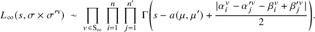(3.7) $$ \begin{align} L_\infty(s, \sigma \times \sigma^{\prime \mathrm{v}}) \ \sim \ \prod_{v \in \mathrm{S}_\infty} \, \prod_{i=1}^n \, \prod_{j=1}^{n'} \ \Gamma\left(s - a(\mu,\mu') + \frac{|\alpha^v_i - \alpha^{\prime v}_j - \beta^v_i + \beta^{\prime v}_j|}{2} \right). \end{align} $$

And similarly,

(3.8) $$ \begin{align} L_\infty(1-s, \sigma^{\mathrm{v}} \times \sigma') \ \sim \ \prod_{v \in \mathrm{S}_\infty} \, \prod_{i=1}^n \, \prod_{j=1}^{n'} \ \Gamma\left(1-s + a(\mu,\mu') + \frac{|\alpha^v_i - \alpha^{\prime v}_j - \beta^v_i + \beta^{\prime v}_j|}{2} \right). \end{align} $$

Let $m \in \tfrac {N}{2} + \mathbb {Z}.$ Then $m \in \mathrm {{Crit}}(\mu ,\mu ')$ if and only if

(3.9) $$ \begin{align} m - a(\mu,\mu') + \frac{|\alpha^v_i - \alpha^{\prime v}_j - \beta^v_i + \beta^{\prime v}_j|}{2} \ \geq \ 1, \quad \forall v \in \mathrm{S}_\infty, \forall i, \forall j, \end{align} $$

which is the condition that $L_\infty (m, \sigma \times \sigma ^{\prime \mathrm {v}})$ is finite from (3.7), and

(3.10) $$ \begin{align} 1-m + a(\mu,\mu') + \frac{|\alpha^v_i - \alpha^{\prime v}_j - \beta^v_i + \beta^{\prime v}_j|}{2} \ \geq \ 1, \quad \forall v \in \mathrm{S}_\infty, \forall i, \forall j, \end{align} $$

which is the condition that $L_\infty (1-m, \sigma ^{\mathrm {v}} \times \sigma ')$ is finite from (3.8). Define the cuspidal width $\ell (\mu ,\mu ')$ between $\mu $ and $\mu '$ as

(3.11) $$ \begin{align} \ell(\mu,\mu') \ := \ \mathrm{min} \left\{|\alpha^v_i - \alpha^{\prime v}_j - \beta^v_i + \beta^{\prime v}_j| \ : \ v \in \mathrm{S}_\infty, 1 \leq i \leq n, \ 1\leq j \leq n' \right\}. \end{align} $$

Then (3.9) and (3.10) together gives us the following

Proposition 3.12. Let $\mu \in X^+_{00}(T_n \times \mathbb {C})$ and $\mu ' \in X^+_{00}(T_{n'} \times \mathbb {C}).$ For $\sigma _f \in \mathrm {{Coh}}_{!!}(G_n, \mu )$ and $\sigma ^{\prime }_f \in \mathrm {{Coh}}_{!!}(G_{n'}, \mu ')$ , the critical set for the Rankin–Selberg L-function $L(s, \sigma \times \sigma ^{\prime \mathrm {v}})$ is given by

$$ \begin{align*}\mathrm{{Crit}}(\mu, \mu') \ = \ \left\{m \in \tfrac{N}{2} + \mathbb{Z} \ : \ 1 - \frac{\ell(\mu,\mu')}{2} + a(\mu, \mu') \ \leq \ m \ \leq \ \frac{\ell(\mu,\mu')}{2} + a(\mu, \mu') \right\}. \end{align*} $$

This is contiguous string of integers or half-integers (depending on whether N is even or odd), centered around $\tfrac 12+ a(\mu , \mu ')$ , of length $\ell (\mu ,\mu ').$

Corollary 3.13. With notations as in Proposition 3.12, the points $s = -N/2$ and $s = 1-N/2$ are both critical for $L(s, \sigma \times \sigma ^{\prime \mathrm {v}})$ if and only if

$$ \begin{align*}- \frac{N}{2} + 1 - \frac{\ell(\mu,\mu')}{2} \ \leq \ a(\mu, \mu') \ \leq \ - \frac{N}{2} -1 + \frac{\ell(\mu,\mu')}{2}. \end{align*} $$

Of course, for this to be possible, one needs $\ell (\mu ,\mu ') \geq 2$ (i.e., that there at least two critical points). The corollary, which is one part of a combinatorial lemma below (Lemma 3.16), is to be viewed like this: the two successive L-values at $s = -N/2$ and $s = 1-N/2$ are critical if and only if the abelian width is bounded in absolute value in terms of the cuspidal width.

Corollary 3.14. Suppose F is in the TR-case and $F_1 = F_0$ is the maximal totally real subfield of F. Given $\mu \in X^+_{00}(T_n \times \mathbb {C})$ and $\mu ' \in X^+_{00}(T_{n'} \times \mathbb {C}),$ if n and $n'$ are both odd, then $\ell (\mu ,\mu ') = 0$ ; in particular, the Rankin–Selberg L-function $L(s, \sigma \times \sigma ^{\prime \mathrm {v}})$ has no critical points.

Proof. Recall from Proposition 2.6 that $\mu $ is the base change of a strongly-pure weight over $F_1$ . For $v \in \mathrm {S}_\infty (F)$ , one has $\eta _v|_{F_1} = \bar {\eta }_v|_{F_1}$ ; hence, $\mu ^{\eta _v} = \mu ^{\bar {\eta }_v}$ . Hence, for the cuspidal parameters, one has $\alpha ^v = w_0 \beta ^v$ ; that is, $\alpha ^v_i = \beta ^v_{n+1-i}.$ If n is odd, then $\alpha ^v_{(n+1)/2} = \beta ^v_{(n+1)/2}.$ Similarly, if $n'$ is odd, then $\alpha ^{\prime v}_{(n'+1)/2} = \beta ^{\prime v}_{(n'+1)/2}.$ From (3.11), it follows that $\ell (\mu ,\mu ') = 0$ , as $0$ is realized as the minimum by taking $i = (n+1)/2$ and $j = (n'+1)/2.$

3.1.3 Critical set at an arithmetic level

Let $\mu \in X^+_{00}(T_n \times E)$ and $\mu ' \in X^+_{00}(T_{n'} \times E),$ and take $\sigma _f \in \mathrm {{Coh}}_{!!}(G_n, \mu )$ and $\sigma ^{\prime }_f \in \mathrm {{Coh}}_{!!}(G_{n'}, \mu ').$ For any $\iota : E \to \mathbb {C}$ , Proposition 3.12 gives the critical set $\mathrm {{Crit}}({}^\iota \mu , {}^\iota \mu ')$ for the Rankin–Selberg L-function $L(s, {}^\iota \sigma \times {}^\iota \sigma ^{\prime \mathrm {v}}).$

Corollary 3.15. The critical set $\mathrm {{Crit}}({}^\iota \mu , {}^\iota \mu ') = \mathrm {{Crit}}(L(s, {}^\iota \sigma \times {}^\iota \sigma ^{\prime \mathrm {v}}))$ is independent of $\iota :$

$$ \begin{align*}\mathrm{{Crit}}(L(s, {}^\iota\sigma \times {}^\iota\sigma^{\prime \mathrm{v}})) \ = \ \mathrm{{Crit}}(L(s, {}^{\gamma \circ\iota}\sigma \times {}^{\gamma \circ\iota}\sigma^{\prime \mathrm{v}})), \quad \forall \ \iota : E \to \mathbb{C}, \ \ \forall \gamma \in \mathrm{{Gal}}(\bar{\mathbb{Q}}/\mathbb{Q}). \end{align*} $$

Proof. From Remark 2.12, one can deduce $\ell ({}^\iota \mu , {}^\iota \mu ') = \ell ({}^{\gamma \circ \iota }\mu , {}^{\gamma \circ \iota }\mu ')$ and $a({}^\iota \mu , {}^\iota \mu ') = a({}^{\gamma \circ \iota }\mu , {}^{\gamma \circ \iota }\mu ').$ One can also see this directly, since by the results of 2.5.3, the archimedean components of ${}^{\gamma \circ \iota }\sigma $ are a permutation of those of ${}^\iota \sigma $ up to conjugates; similarly, for ${}^\iota \sigma '$ ; since $L(s, z^\alpha \bar {z}^\beta ) = L(s, z^\beta \bar {z}^\alpha )$ , one gets $L_\infty (s, {}^\iota \sigma \times {}^\iota \sigma ^{\prime \mathrm {v}}) = L_\infty (s, {}^{\gamma \circ \iota }\sigma \times {}^{\gamma \circ \iota }\sigma ^{\prime \mathrm {v}}).$

3.2 Combinatorial lemma

3.2.1 Statement of the lemma

Lemma 3.16. For strongly-pure weights $\mu \in X^+_{00}(T_n \times \mathbb {C})$ and $\mu ' \in X^+_{00}(T_{n'} \times \mathbb {C})$ , and cuspidal Hecke summands $\sigma _f \in \mathrm {{Coh}}_{!!}(G_n, \mu )$ , $\sigma ^{\prime }_f \in \mathrm {{Coh}}_{!!}(G_{n'}, \mu '),$ the following are equivalent:

1. 1. The points $s = -N/2$ and $s = 1-N/2$ are both critical for $L(s, \sigma \times \sigma ^{\prime \mathrm {v}})$ .

2. 2. The abelian width is bounded in terms of the cuspidal width as

   $$ \begin{align*}- \frac{N}{2} + 1 - \frac{\ell(\mu,\mu')}{2} \ \leq \ a(\mu, \mu') \ \leq \ - \frac{N}{2} -1 + \frac{\ell(\mu,\mu')}{2}. \end{align*} $$

3. 3. There exists $w \in W^P$ such that $w^{-1}\cdot (\mu +\mu ')$ is dominant and $l(w^\eta ) + l(w^{\bar {\eta }}) = \dim (U_{P_0})$ for all $\eta : F \to \mathbb {C}.$ (Recall: $w = (w^\eta )_{\eta : F \to \mathbb {C}}$ with $w^\eta \in W^{P_0 \times _\eta \mathbb {C}} \subset W_{G_0} \times _\eta \mathbb {C}$ .)

We have already proved $(1) \iff (2)$ . It remains to prove $(2) \iff (3).$ It is clear that

$$ \begin{align*}l(w^\eta) + l(w^{\bar{\eta}}) = \dim(U_{P_0}), \ \forall \eta : F \to \mathbb{C} \ \implies \ l(w) = \tfrac12 \dim(U_P). \end{align*} $$

However, if the degree of F is greater than $2$ (i.e., if ${\mathrm r}> 1$ ), then the converse is not true in general.

Definition 3.17. A Kostant representative $w \in W^P$ is said to be balanced if

$$ \begin{align*}l(w^\eta) + l(w^{\bar{\eta}}) = \dim(U_{P_0}), \ \forall \eta : F \to \mathbb{C}.\end{align*} $$

For the benefit of the reader, we will make two passes over the proof of (2) $\iff $ (3) in simpler situations, because the proof in the general case is intricate in details and somewhat tedious; it is the sort of proof that makes one believe the dictum ‘der Teufel steckt im Detail’.

3.2.2 Explicating (2) $\iff $ (3) in the simplest nontrivial example

Proof. Let us consider the case of $n = n' = 1$ and so $N = 2.$ Take F to be an imaginary quadratic field with $\mathrm {{Hom}}(F,\mathbb {C}) = \{\eta , \bar {\eta }\}.$ The weights $\mu $ and $\mu '$ are both a pair of integers indexed by $\mathrm {{Hom}}(F,\mathbb {C});$ we will write $ \mu \ = \ ((a), (a^{*})), \quad \mu ' \ = \ ((b), (b^{*})), $ with $a,a^{*}, b, b^{*} \in \mathbb {Z},$ with the convention that $\mu ^\eta = (a), \mu ^{\bar {\eta }} = (a^{*})$ and similarly for $\mu '.$ Note that purity of $\mu $ and $\mu '$ is automatic, and the purity weights are $\mathbf {{w}} = a+a^{*}, \ \mathbf {{w}}' = b+b^{*}.$ The abelian width is $a(\mu , \mu ') = \frac {a+a^{*} - b-b^{*}}{2}.$ The cuspidal parameters at the only complex place v of F are $\alpha ^v = (-a), \ \beta ^v = (-a^{*}), \ \alpha ^{\prime v} = (-b), \ \beta ^{\prime v} = (-b^{*}).$ The cuspidal width is $\ell (\mu , \mu ') = |-a+a^{*} +b-b^{*}|.$ The weight $\mu +\mu '$ which we would like make dominant using a balanced Kostant representative has the shape $\mu +\mu ' \ = \ ((a,b), \, (a^{*}, b^{*})).$ For simplicity, let us denote $p := a-b, \ p^{*} := a^{*} - b^{*}.$ Hence, $\mu +\mu '$ is dominant if and only if $p \geq 0$ and $p^{*} \geq 0.$ The inequalities in (2) now take the shape

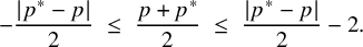(3.18) $$ \begin{align} - \frac{|p^{*}-p|}{2} \ \leq \ \frac{p+p^{*}}{2} \ \leq \ \frac{|p^{*}-p|}{2} - 2. \end{align} $$

Since, $P_0 = B_0$ is the Borel subgroup, the Levi subgroup $M_P$ is a torus; hence, $W_{M_P}$ is trivial and $W^P = W_G.$ If $W_{G_0}$ is written as $\{1,s\}$ with s the nontrivial element, then the elements of $W^P$ may be written as $ W_G = (\{1,s\}, \{1^{*}, s^{*}\}). $ The dimension of $U_P$ is $2$ ; hence, the balanced elements (of length $1$ ) of $W^P$ are $(1,s^{*})$ and $(s,1)$ . Now, consider three cases depending on the sign of $p - p^{*}$ :

• ○ $p=p^{*}.$ In this case, (3.18) reads $0 \leq p \leq -2,$ which is absurd; hence, (2) is violated. If $p \geq 0$ , then the only $w \in W^P$ such that $w^{-1}\cdot (\mu +\mu ')$ is dominant is $w = (1,1^{*})$ which has length $0$ ; hence, (3) is violated. Similarly, if $p < 0$ , then the only $w \in W^P$ such that $w^{-1}\cdot (\mu +\mu ')$ is dominant is $w = (s,s^{*}),$ which has length $2$ ; hence, (3) is violated again. So, both (2) and (3) are false.

• ○ $p>p^{*}.$ In this case, (3.18) simplifies to $p^{*} - p \leq p + p^{*} \leq p - p^{*} - 4,$ which implies that $p \geq 0> -2 \geq p^{*}.$ The only $w \in W^P$ such that $w^{-1}\cdot (\mu +\mu ')$ is dominant is $w = (1,s^{*})$ which has length $1$ ; hence, (3) is satisfied.

• ○ $p<p^{*}.$ In this case, $p^{*} \geq 0> -2 \geq p$ and the only $w \in W^P$ that works is $(s,1)$ which is of length $1$ .

In all cases, either both (2) and (3) are satisfied, or both are violated. Hence, $(2) \iff (3).$

In the second case ( $p>p^{*}$ ), one might ask what happens in the degenerate case of $p=0$ and $p^{*}=-1.$ (So we are violating (2) but keeping $p>p^{*}$ .) This means that $\mu +\mu '$ has the shape $((a,a), (b^{*}-1,b^{*}))$ . The $\eta $ component $(a,a)$ is dominant, but one has to make the $\bar {\eta }$ -component $(b^{*}-1,b^{*})$ dominant. This can only be done using $s^{*}$ ; however, the reader can easily check that $s^{*} \cdot (b^{*}-1,b^{*}) = (b^{*}-1,b^{*})$ . In other words, there is no element w such that $w^{-1}\cdot (\mu +\mu ')$ is dominant.

3.2.3 Proof of (2) $\iff $ (3) for $\mathrm {{GL}}_n \times \mathrm {{GL}}_1$

It is most convenient to first understand the case when F is an imaginary quadratic field. Then $\Sigma _F = \{\eta , \bar {\eta }\}$ (for a non-canonical choice of $\eta : F \to \mathbb {C}$ that is fixed once and for all). As above, we will follow a notational artifice that all quantities indexed by $\bar {\eta }$ will be designated with a $*$ . A weight $\mu \in X^+_{0}(T_n \times \mathbb {C})$ may be written as $\mu = \{ \mu ^\eta , \mu ^{\bar {\eta }} \}$ with $\mu ^\eta = (\mu _1 \geq \mu _2 \geq \cdots \geq \mu _n)$ and $\mu ^{\bar {\eta }} = (\mu _1^{*} \geq \mu _2^{*} \geq \cdots \geq \mu _n^{*}),$ with $\mu _i, \mu _j^{*} \in \mathbb {Z},$ and purity implies $\mathbf {{w}} \ = \ \mu _i + \mu _{n-i+1}^{*}.$ A weight $\mu ' \in X^+_{0}(T_1 \times \mathbb {C})$ is simply a pair of integers $\mu ' = \{b, b^{*}\}$ with purity weight $\mathbf {{w}}' = b+b^{*}$ . The weight $\mu +\mu '$ is given by

$$ \begin{align*}\mu + \mu' \ = \ \{(\mu_1, \mu_2, \dots, \mu_n, b), \quad (\mu_1^{*}, \mu_2^{*}, \dots, \mu_n^{*}, b^{*}) \}. \end{align*} $$

We are seeking to understand when we can find a Kostant representative $w \in W^P$ which is balanced ( $l(w^\eta ) + l(w^{\bar {\eta }})= \dim (U_{P_0}) = n$ ) and such that $w^{-1}\cdot (\mu + \mu ')$ is a dominant weight. For this, first identify the Kostant representatives for $P_0$ in $G_0$ ; the simple roots of $M_{P_0}$ are $\mathbf {\Pi }_{M_{P_0}} = \{e_1-e_2, e_2-e_3, \, \dots , e_{n-1} - e_n\}.$ The Weyl group of $G_0$ is $W_{G_0} = \mathfrak {S}_{n+1}$ the symmetric group on $n+1$ letters. We have

$$ \begin{align*} w \in W^{P_0} & \iff w^{-1}(e_1-e_2)> 0, \ w^{-1}(e_2-e_3) > 0, \ \dots, w^{-1}(e_{n-1} - e_n) > 0 \\ & \iff w^{-1}(1) < w^{-1}(2) < \cdots < w^{-1}(n). \end{align*} $$

The elements of $W^{P_0}$ and their lengths are listed below:

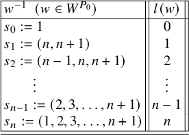$$ \begin{align*}\begin{array}{|l||c||} \hline w^{-1} \ \ (w\in W^{P_0}) & l(w) \\ \hline s_0 := 1 & 0 \\ s_1 := (n, n+1) & 1 \\ s_2 := (n-1, n, n+1) & 2 \\ \quad \quad \vdots & \vdots \\ s_{n-1} := (2,3,\dots, n+1) & n-1 \\ s_n := (1,2,3,\dots, n+1) & n \\ \hline \hline \end{array} \end{align*} $$

Note that the $(n+1)$ -cycle $(1,2,\dots ,n+1) = (1,2)(2,3)\cdots (n,n+1)$ as a product of n simple transpositions giving its length which applies to the last row and a similar calculation gives all the other lengths. The Kostant representatives for P are $W^P \ = \ \{(w, w^{*}) \ : \ w , w^{*} \in W^{P_0}\},$ where $l(w,w^{*}) = l(w) + l(w^{*}).$ Hence, the inverses of the balanced Kostant representatives are

$$ \begin{align*}\{(s_0, s_n^{*}), \ (s_1, s_{n-1}^{*}), \dots, (s_n, s_0^{*}) \}. \end{align*} $$

The twisted action of the Kostant representatives on the weight are given in the table below:

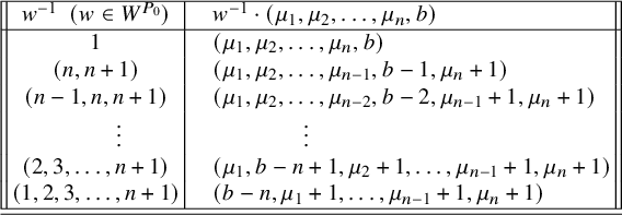(3.19) $$ \begin{align} \begin{array}{||c|l||} \hline w^{-1} \ \ (w\in W^{P_0}) & \quad w^{-1} \cdot (\mu_1,\mu_2,\dots, \mu_n,b) \\ \hline 1 & \quad (\mu_1,\mu_2,\dots, \mu_n, b) \\ (n, n+1) & \quad (\mu_1,\mu_2,\dots, \mu_{n-1}, b-1, \mu_n +1) \\ (n-1, n, n+1) & \quad (\mu_1,\mu_2,\dots, \mu_{n-2}, b-2, \mu_{n-1} +1, \mu_n +1) \\ \quad \quad \vdots & \quad\quad\quad \quad\quad\vdots \\ (2,3,\dots, n+1) & \quad (\mu_1, b-n+1, \mu_2 +1 ,\dots, \mu_{n-1} +1, \mu_n +1) \\ (1,2,3,\dots, n+1) & \quad (b-n, \mu_1+1, \dots, \mu_{n-1} +1, \mu_n +1)\\ \hline \hline \end{array} \end{align} $$

For the combinatorial lemma (Lemma 3.16), the abelian width is given by

$$ \begin{align*}a(\mu, \mu') \ = \ \frac{\mathbf{{w}} - \mathbf{{w}}'}{2} \ = \ \frac{\mu_i + \mu_{n-i+1}^{*} - b - b^{*}}{2} \ = \ \frac{(\mu_i - b) + (\mu_{n-i+1}^{*} - b^{*})}{2}, \end{align*} $$

and for the cuspidal width, the cuspidal parameters are given by

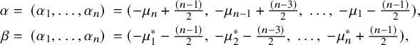$$ \begin{align*} \alpha = \ (\alpha_1,\dots, \alpha_n) \ = & \ (-\mu_n+ \tfrac{(n-1)}{2}, \ -\mu_{n-1}+\tfrac{(n-3)}{2},\ \dots, \ -\mu_1-\tfrac{(n-1)}{2}), \\ \beta = \ (\alpha_1,\dots, \alpha_n) \ = & \ (-\mu_1^{*}-\tfrac{(n-1)}{2}, \ -\mu_2^{*}-\tfrac{(n-3)}{2},\ \dots, \ -\mu_n^{*}+\tfrac{(n-1)}{2}), \end{align*} $$

and similarly, $ \alpha ' = -b, \ \beta ' = -b^{*},$ from which the cuspidal width is

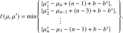$$ \begin{align*}\ell(\mu,\mu') = \min\left\{ \begin{array}{l} |\mu_1^{*}-\mu_n+(n-1) +b -b^{*}|, \\ |\mu_2^{*}-\mu_{n-1}+(n-3) +b -b^{*}|, \\ \quad \quad \quad \vdots \\ |\mu_n^{*}-\mu_1-(n-1) +b -b^{*}| \end{array}\right\}. \end{align*} $$

From the shape of $a(\mu ,\mu ')$ and $\ell (\mu , \mu ')$ , it is convenient to introduce the quantities $c_i := \mu _i - b$ and $c_i^{*} := \mu _i^{*}-b^{*}.$ (These are the p and $p^{*}$ when $n=1$ .) Then we have $a(\mu , \mu ') = \frac {c_i + c_{n-i+1}^{*}}{2},$ and

$$ \begin{align*}\ell(\mu,\mu') \ = \ \min\{ \ |c_1^{*}-c_n + (n-1)|, \ |c_2^{*}-c_{n-1}+(n-3)|, \ |c_n^{*} - c_1 - (n-1)| \ \}. \end{align*} $$

From the dominance of the weights $\mu $ and $\mu '$ , we have the inequalities

$$ \begin{align*}c_1^{*}-c_n + (n-1) \> \ c_2^{*}-c_{n-1}+(n-3) \ > \ \cdots \ > c_n^{*} - c_1 - (n-1). \end{align*} $$

The proof conveniently breaks into $(n+1)$ disjoint cases depending on the relative position of $0$ in the above decreasing sequence.

Case 0: $0> c_1^{*}-c_n + (n-1) \ > \ c_2^{*}-c_{n-1}+(n-3) \ > \ \cdots \ > c_n^{*} - c_1 - (n-1),$

Case j ( $1\ \leq j \leq n-1$ ): $c_j^{*}-c_{n-j+1} + (n-2j+1) \> 0 \ > \ c_{j+1}^{*}-c_{n-j}+(n-2j-1),$

Case n: $c_1^{*}-c_n + (n-1) \> \ c_2^{*}-c_{n-1}+(n-3) \ > \ \cdots \ > c_n^{*} - c_1 - (n-1) > 0.$

In Case 0, we have $\ell (\mu ,\mu ') = -c_1^{*}+c_n - (n-1).$ Keeping in mind that $N = n+1$ , the inequalities in (2) of the lemma read

$$ \begin{align*}- \frac{(n+1)}{2} + 1 - \frac{(-c_1^{*}+c_n-(n-1))}{2} \ \leq \ \frac{c_1^{*}+c_n}{2} \ \leq \ - \frac{(n+1)}{2} -1 + \frac{(-c_1^{*}+c_n-(n-1))}{2} \end{align*} $$

This simplifies to

$$ \begin{align*}c_1^{*}-c_n \ \leq \ c_1^{*} + c_n \ \leq \ -c_1^{*} + c_n - 2n - 2. \end{align*} $$

Whence we get

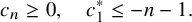$$ \begin{align*}c_n \geq 0, \quad c_1^{*} \leq -n-1. \end{align*} $$

This is exactly the condition that $w^{-1} = (1, s_n^{*})$ under the twisted action makes $\mu +\mu '$ dominant. (See the last row of (3.19).)

Case n is similar; we have $\ell (\mu ,\mu ') = c_n^{*}-c_1 - (n-1).$ The inequalities in (2) of the lemma read

$$ \begin{align*}- \frac{(n+1)}{2} + 1 - \frac{(c_n^{*}-c_1 - (n-1))}{2} \ \leq \ \frac{c_n^{*}+c_1}{2} \ \leq \ - \frac{(n+1)}{2} -1 + \frac{(c_n^{*}-c_1 - (n-1))}{2} \end{align*} $$

This simplifies to

$$ \begin{align*}-c_n^{*}+c_1 \ \leq \ c_n^{*} + c_1 \ \leq \ c_n^{*} - c_1 - 2n - 2. \end{align*} $$

Whence we get

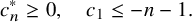$$ \begin{align*}c_n^{*} \geq 0, \quad c_1 \leq -n-1. \end{align*} $$

This is exactly the condition that $w^{-1} = (s_n, 1^{*})$ makes $\mu +\mu '$ dominant.

Case j breaks up into two sub-cases:

1. Case j1: $c_j^{*}-c_{n-j+1} + (n-2j+1) \geq c_{n-j} - c_{j+1}^{*} - (n-2j-1).$

2. Case j2: $c_j^{*}-c_{n-j+1} + (n-2j+1) < c_{n-j} - c_{j+1}^{*} - (n-2j-1).$

For j1, we have $\ell (\mu ,\mu ') = c_{n-j} - c_{j+1}^{*} - (n-2j-1)$ and the inequalities of (2) read

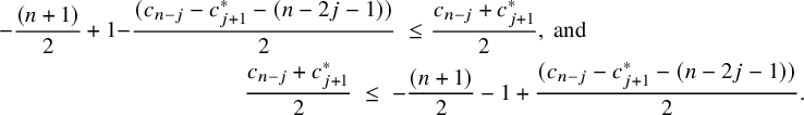$$ \begin{align*} - \frac{(n+1)}{2} + 1 - &\frac{(c_{n-j} - c_{j+1}^{*} - (n-2j-1))}{2} \ \leq\frac{c_{n-j} + c_{j+1}^{*}}{2}, \ \mathrm{and} \\ &\qquad\qquad\quad \frac{c_{n-j} + c_{j+1}^{*}}{2} \ \leq \ - \frac{(n+1)}{2} -1 + \frac{(c_{n-j} - c_{j+1}^{*} - (n-2j-1))}{2}. \end{align*} $$

These simplify to

$$ \begin{align*}- c_{n-j} + c_{j+1}^{*} - 2j \ \leq \ c_{n-j} + c_{j+1}^{*} \ \leq \ c_{n-j} - c_{j+1}^{*} - 2n+2j-2.\end{align*} $$

This in turn implies that

$$ \begin{align*}c_{n-j} \ \geq \ -j, \quad c_{j+1}^{*} \ \leq \ -n+j-1. \end{align*} $$

Next, we see that the defining inequalities of j1 gives in particular that

(3.20) $$ \begin{align} c_j^{*} + c_{j+1}^{*} + 2n-4j \ \geq \ c_{n-j} + c_{n-j+1}. \end{align} $$

Add $c_{n-j+1}$ on both sides of (3.20) to get

$$ \begin{align*}c_{n-j+1} + c_j^{*} + c_{j+1}^{*} + 2n-4j \ \geq \ c_{n-j} + 2c_{n-j+1}, \end{align*} $$

and applying purity, we can rewrite this as

$$ \begin{align*}c_{n-j} + 2c_{j+1}^{*}+ 2n-4j \ \geq \ c_{n-j} + 2c_{n-j+1}, \end{align*} $$

whence

$$ \begin{align*}c_{n-j+1} \ \leq \ c_{j+1}^{*}+ n-2j \ \leq \ -j-1. \end{align*} $$

Next, add $c_j^{*}$ to both sides of (3.20) to get

$$ \begin{align*}2c_j^{*} + c_{j+1}^{*} + 2n-4j \ \geq \ c_{n-j} + c_{n-j+1} + c_j^{*}, \end{align*} $$

and applying purity, we can rewrite this as

$$ \begin{align*}2c_j^{*} + c_{j+1}^{*}+ 2n-4j \ \geq \ 2c_{n-j} + c_{j+1}^{*} \end{align*} $$

whence,

$$ \begin{align*}c_j^{*} \ \geq \ c_{n-j} - n + 2j \ \geq \ -n+j. \end{align*} $$

Putting all this together, we get the following inequalities:

$$ \begin{align*}c_{n-j} \geq -j, \quad c_{n-j+1} \leq -j-1, \quad \mathrm{and} \quad c_j^{*} \geq j-n, \quad c_{j+1}^{*} \leq -n+j-1. \end{align*} $$

For j2, we have $\ell (\mu ,\mu ') = c_j^{*} - c_{n-j+1} + (n-2j+1)$ and the inequalities of (2) simplifying to

$$ \begin{align*}c_j^{*} \geq -n+j \quad \mathrm{and} \quad c_{n-j+1} \leq -j-1. \end{align*} $$

The defining inequalities of j2 may be written as

(3.21) $$ \begin{align} c_j^{*} + c_{j+1}^{*} \ \leq \ c_{n-j} + c_{n-j+1} -2n+4j. \end{align} $$

Add $c_{j+1}^{*}$ to both sides of (3.21), apply purity to the right-hand side, and simplify to get

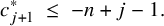$$ \begin{align*}c_{j+1}^{*} \ \leq \ -n+j-1. \end{align*} $$

Next, add $c_{n-j}$ to both sides of (3.21), apply purity to the left-hand side, and simplify to get

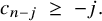$$ \begin{align*}c_{n-j} \ \geq \ -j. \end{align*} $$

Putting all this together, we see exactly as in Case j1 that

$$ \begin{align*}c_{n-j} \geq -j, \quad c_{n-j+1} \leq -j-1, \quad \mathrm{and} \ c_j^{*} \geq -n+j, \quad c_{j+1}^{*} \leq -n+j-1. \end{align*} $$

Using the table (3.19), we see that

$$ \begin{align*}c_{n-j} \geq -j, \quad c_{n-j+1} \leq -j-1 \ \iff \ s_j \cdot (\mu_1,\dots,\mu_n,b) \ \mbox{is dominant}. \end{align*} $$

$$ \begin{align*}c_j^{*} \geq j-n, \quad c_{j+1}^{*} \leq -n+j-1 \ \iff \ s_{n-j}^{*} \cdot (\mu_1^{*},\dots,\mu_n^{*},b^{*}) \ \mbox{is dominant}. \end{align*} $$

So, in Case j, the required balanced Kostant representative is the inverse of $(s_j, s_{n-j}^{*}).$

Conversely, if $w^{-1} = (s_j, s_{n-j}^{*})$ makes $(\mu +\mu ')$ dominant, then we just argue backwards in the above paragraphs to see that inequalities of (2) are satisfied. Thus far, we have proved (2) $\iff $ (3) when F is imaginary quadratic.

A general totally imaginary field

Now let F be any totally imaginary field. For each $v \in \mathrm {S}_\infty $ we have a pair of complex embeddings $\{\eta _v, \bar {\eta }_v\}$ of F. For any such embedding $\eta $ , the weight $\mu $ , has a $\eta $ -component $\mu ^\eta = (\mu ^\eta _1,\dots ,\mu ^\eta _n)$ which is a non-increasing sequence of integers, and similarly, $\mu ^{\prime \eta } = (b^\eta )$ is just an integer. Define $c_j^\eta = \mu ^\eta _j - b^\eta $ . The abelian width is given by $a(\mu , \mu ') \ = \ \frac {c_j^\eta + c_{n-j+1}^{\bar {\eta }}}{2},$ for any j and any $\eta .$ For $v \in \mathrm {S}_\infty $ , define $\ell _v(\mu ,\mu ')$ as the minimum of the absolute values of the following n integers:

$$ \begin{align*}c^{\bar{\eta}_v}_1- c^{\eta_v}_n + (n-1) \> \ c^{\bar{\eta}_v}_2-c_{n-1}^{\eta_v}+(n-3) \ > \ \cdots \ > c^{\bar{\eta}_v}_n - c_1^{\eta_v} - (n-1). \end{align*} $$

Then $\ell (\mu ,\mu ') = \min \{\ell _v(\mu ,\mu ') \, : \, v \in \mathrm {S}_\infty \}.$ The inequalities of (2) imply that for each $v \in \mathrm {S}_\infty $ , we have

(3.22) $$ \begin{align} - \frac{N}{2} + 1 - \frac{\ell_v(\mu,\mu')}{2} \ \leq \ a(\mu, \mu') \ \leq \ - \frac{N}{2} -1 + \frac{\ell_v(\mu,\mu')}{2}. \end{align} $$

Using the same argument as in the imaginary quadratic case, we see that there exists $ w_v \ = \ (w_{\eta _v}, w_{\bar {\eta }_v}) \ \in \ W^{(P_0 \times _{\eta _v} \mathbb {C}) \times (P_0 \times _{\bar {\eta }_v} \mathbb {C})} $ such that $w_v^{-1}\cdot ((\mu ^{\eta _v}, \mu ^{\prime \eta _v}), (\mu ^{\bar {\eta }_v}, \mu ^{\prime \bar {\eta }_v}))$ is dominant and $l(w_{\eta _v}) + l(w_{\bar {\eta }_v}) = n.$ The required balanced Kostant representative then is $w = (w_v)_{v \in \mathrm {S}_\infty }$ ; hence, (3) is satisfied. Conversely, if (3) holds, then writing $w = (w^\eta )$ as $w = (w_v)$ with $w_v = (w_{\eta _v}, w_{\bar {\eta }_v})$ , we see that $w_v^{-1}\cdot ((\mu ^{\eta _v}, \mu ^{\prime \eta _v}), (\mu ^{\bar {\eta }_v}, \mu ^{\prime \bar {\eta }_v}))$ is dominant, and working backwards as in the imaginary quadratic case, we deduce (3.22) holds for each v, and hence, (2) holds. $\Box $

3.2.4 Proof of (2) $\iff $ (3) in the general case

First of all, we will prove it in the special case when F is imaginary quadratic (i.e., ${\mathfrak {r}} = 1).$

Parametrizing Kostant representatives

We will need explicit Kostant representatives. Recall that $G_0 = \mathrm {{GL}}_N$ and $P_0 = M_{P_0} U_{P_0}$ the standard $(n, n')$ -parabolic subgroup of $G_0$ , where $N = n+n';$ clearly, $\dim (U_{P_0}) = nn'.$ Then $W_{G_0} = \mathfrak {S}_N$ the permutation group on N letters, and $W_{M_{P_0}} = \mathfrak {S}_n \times \mathfrak {S}_{n'}.$ The set of Kostant representatives $W^{P_0}$ may be described as

(3.23) $$ \begin{align} W^{P_0} \ = \ \{w \in W_{G_0} \ : \ w^{-1}(1) < \cdots < w^{-1}(n) \ \mathrm{and} \ w^{-1}(n+1) < \cdots < w^{-1}(N) \}. \end{align} $$

The set $W^{P_0}$ is in bijection with the set of all n-tuples $\kappa = (k_1,\dots , k_n)$ , where $1 \leq k_1 < \cdots < k_n \leq N$ . Any such $\kappa $ corresponds to $w_\kappa \in W^{P_0}$ , which is uniquely defined by the conditions

(3.24) $$ \begin{align} w_\kappa^{-1}(1) = k_1, \, \dots, w_\kappa^{-1}(n) = k_n. \end{align} $$

If $\kappa = (1,2,\dots , n)$ , then $w_\kappa $ is the identity element. There is a self-bijection $W^{P_0} \to W^{P_0}$ defined by $w_\kappa \mapsto w_{\kappa ^{\mathrm {v}}}$ , where

(3.25) $$ \begin{align} \kappa^{\mathrm{v}} \ := \ N+1-k_n \ < \ \cdots \ < N+1 - k_1; \quad \kappa^{\mathrm{v}}_j = N+1 - k_{n-j+1}. \end{align} $$

Let $w_N = w_{G_0} \in W_{G_0}$ denote the element of longest length, which is given by $w_N(j) = N+1-j$ for any $1 \leq j \leq N$ ; clearly, $w_{G_0}^2 = 1.$ Similarly, $w_n$ and $w_{n'}$ are defined, and we have $w_{M_{P_0}} = w_n \times w_{n'}$ .

Lemma 3.26. With the notations as above, we have

1. 1. $l(w_\kappa ) = (k_1-1) + (k_2-2) + \dots + (k_n-n).$

2. 2. $l(w_\kappa ) + l(w_{\kappa ^{\mathrm {v}}}) = nn' = \dim (U_{P_0}).$

3. 3. $w_{\kappa ^{\mathrm {v}}} = w_{M_{P_0}} w_\kappa w_{G_0}.$

Proof. Clearly, $l(w_\kappa ) = l(w_\kappa ^{-1})$ , and for counting the length of $w_\kappa ^{-1}$ , count the number of its shuffles – that is, count the number of pairs $(i,j)$ with $1 \leq i < j \leq N$ with $w_\kappa ^{-1}(i)> w_\kappa ^{-1}(j).$ But for any such shuffle, by (3.23), it is clear that $1 \leq i \leq n$ and $n+1 \leq j \leq N$ . We leave it to the reader to see that for a fixed $i \leq n$ , the number of shuffles $(i,j)$ is $k_i - i$ . Also, (2) follows from Statement (1) and (3.25). To see the validity of (3), compute the inverses of both sides on any $1 \leq j \leq n$ :

$$ \begin{align*}(w_{G_0} w_\kappa^{-1} w_{M_{P_0}})(j) = ( w_{G_0} w_\kappa^{-1})(n+1-j) = w_{G_0}(k_{n+1-j}) = N+1-k_{n+1-j} = \kappa^{\mathrm{v}}_j = w_{\kappa^{\mathrm{v}}}^{-1}(j).\\[-37pt] \end{align*} $$

Twisted action of $W^{P_0}$ on weights

The usual permutation action of $\sigma \in S_m$ on an m-tuple is given by $\sigma (t_1,\dots , t_m) \ = \ (t_{\sigma ^{-1}(1)}, \dots , t_{\sigma ^{-1}(m)}).$ If $\underline {t} := (t_1,\dots , t_m)$ , then the twisted action of $\sigma $ on $\underline {t}$ is defined by which unravels to

$$ \begin{align*}\sigma \cdot (t_1,\dots, t_m) \ = \ (t_{\sigma^{-1}(1)} + 1 - \sigma^{-1}(1), \, t_{\sigma^{-1}(2)} + 2 - \sigma^{-1}(2), \, \dots, \, t_{\sigma^{-1}(m)}+ m - \sigma^{-1}(m)). \end{align*} $$

Now, keeping the combinatorial lemma (Lemma 3.16) in mind, suppose

$$ \begin{align*}\mu = ((b_1,\dots,b_n), \, (c_1,\dots, c_n)), \quad \mu' = ((b^{\prime}_1,\dots,b^{\prime}_{n'}), \, (c^{\prime}_1,\dots, c^{\prime}_{n'})), \end{align*} $$

where each n-tuple or $n'$ -tuple is a non-increasing string of integers satisfying the purity condition $\mathbf {{w}} = b_i + c_{n-i+1}, \ \mathbf {{w}}' = b^{\prime }_j + c^{\prime }_{n'-j+1}.$ We are seeking a Kostant representative of optimal length that ‘straightens out’

$$ \begin{align*}\mu+\mu' \ = \ ((b_1,\dots,b_n, b^{\prime}_1,\dots,b^{\prime}_{n'}), \, (c_1,\dots, c_n, c^{\prime}_1,\dots, c^{\prime}_{n'})). \end{align*} $$

For this, we need the twisted action of $w_\kappa ^{-1}$ on an $(n+n')$ -tuple like $(b_1,\dots ,b_n, b^{\prime }_1,\dots ,b^{\prime }_{n'})$ . Given $\kappa $ , let us define its complement $\kappa ^c$ as the ordered string of integers:

$$ \begin{align*}\kappa^c \ := \ k^c_1 < \cdots < k^c_{n'} \ := \ \{1,2,\dots, N\} \setminus \{k_1, k_2, \dots, k_n\}. \end{align*} $$

It is useful to note that

$$ \begin{align*}\kappa^c \ = \ \{1, 2, \dots, k_1-1, k_1+1, \dots , k_2-1, k_2+1, \dots, k_n-1, k_n+1, \dots, N \}. \end{align*} $$

The element $w_\kappa ^{-1} \in W^{P_0}$ is the permutation that may be written as

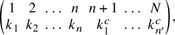$$ \begin{align*}\begin{pmatrix} 1 & 2 & \dots & n & n+1 & \dots & N \\ k_1 & k_2 & \dots & k_n & k^c_1 & \dots & k^c_{n'} \end{pmatrix}, \end{align*} $$

and the permutation $w_\kappa $ is

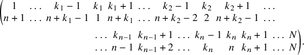$$ \begin{align*} &\left(\begin{matrix} 1 & \dots & k_1-1 & k_1 & k_1+1 & \dots & k_2-1 & k_2 & k_2+1 &\dots \\ n+1 & \dots & n+ k_{1}-1 & 1 & n+k_1 & \dots & n+k_2-2 & 2 & n+k_2-1 & \dots \end{matrix}\right. \\ &\qquad\qquad\qquad\qquad\quad\left. \begin{matrix} \dots & k_{n-1} & k_{n-1}+1 & \dots & k_n-1 & k_n & k_n+1 & \dots & N\\ \dots & n-1 & k_{n-1}+2 & \dots & k_n & n & k_n+1 & \dots & N \end{matrix} \right). \end{align*} $$

(The reader should pay some attention to the special cases $k_1 = 1$ and $k_n = N$ .) Denoting

$$ \begin{align*}(b_1,\dots,b_n, b^{\prime}_1,\dots,b^{\prime}_{n'}) \ = \ (d_1,\dots,d_n, d_{n+1}, \dots, d_N), \end{align*} $$

we have

(3.27) $$ \begin{align} w_\kappa^{-1} \cdot &(d_1,\dots,d_n, d_{n+1}, \dots, d_N) \ = \notag\\ &\qquad\qquad\qquad\quad (d_{w_\kappa(1)}+1- w_\kappa(1), \ d_{w_\kappa(2)}+2- w_\kappa(2), \ \dots \ , d_{w_\kappa(N)}+N- w_\kappa(N)). \end{align} $$

Dominance of $w_\kappa ^{-1} \cdot (d_1,\dots ,d_N)$

Let us enumerate the inequalities that guarantee dominance of the weight in (3.27):

Proposition 3.28. The weight $w_\kappa ^{-1} \cdot (d_1,\dots ,d_n, d_{n+1}, \dots , d_N)$ is dominant if and only if the following conditions are satisfied:

1. (0) If $k_1 - 1 \geq 1$ , then

   $$ \begin{align*}b^{\prime}_{k_1-1} - b_1 \ \geq \ n+k_1-1.\end{align*} $$
   If $k_1=1$ , then there is no such condition.

2. (1) If $k_2 \geq k_1+2$ , then

   1. (i)

      $$ \begin{align*}b_1-b^{\prime}_{k_1} \ \geq \ -n-k_1+2,\end{align*} $$
      and

   2. (ii)

      $$ \begin{align*}b^{\prime}_{k_2-2} - b_2 \ \geq \ n+ k_2-3.\end{align*} $$

   If $k_2 = k_1+1$ , then there are no such conditions.

3. $$ \begin{align*}\vdots\end{align*} $$

4. (l) ( $1 \leq l \leq n-1$ ) If $k_{l+1} \geq k_l+2$ , then

   1. (i)

      $$ \begin{align*}b_l - b^{\prime}_{k_l+1-l} \ \geq \ -n -k_l +2l,\end{align*} $$
      and

   2. (ii)

      $$ \begin{align*}b^{\prime}_{k_{l+1}-l-1} - b_{l+1} \ \geq \ n + k_{l+1} -2l -1.\end{align*} $$

   If $k_{l+1} = k_l+1$ , then there are no such conditions.

5. $$ \begin{align*}\vdots\end{align*} $$

6. (n – 1) If $k_n \ \geq \ k_{n-1}+2$ , then

   1. (i)

      $$ \begin{align*}b_{n-1} - b^{\prime}_{k_{n-1}+2-n} \ \geq \ n- k_{n-1}-2,\end{align*} $$
      and

   2. (ii)

      $$ \begin{align*}b^{\prime}_{k_n-n} - b_n \ \geq \ -n + k_n + 1.\end{align*} $$

   If $k_n = k_{n-1}+1$ , then there are no such conditions.

7. (n) If $k_n \leq N-1$ , then

   $$ \begin{align*}b_n - b^{\prime}_{k_n+1-n} \ \geq \ n-k_n \end{align*} $$
   If $k_n = N$ , then there is no such condition.

In the above $n+1$ conditions, some of them might be empty; however, not all can be empty.

Proof. The tedious argument has the same flavour for each case $(1), (2), \dots (l), \dots (n-1), (n)$ ; as a representative, let us verify (1). If $k_2 \geq k_1+2$ , then looking at the relevant part of $w_\kappa $ ,

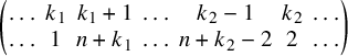$$ \begin{align*}\begin{pmatrix} \dots & k_1 & k_1+1 & \dots & k_2-1 & k_2 & \dots \\ \dots & 1 & n+k_1 & \dots & n+k_2-2 & 2 & \dots \end{pmatrix} \end{align*} $$

we will have two dominance conditions: comparing entries at steps $k_1$ and $k_1+1$ gives

(3.29) $$ \begin{align} d_{w_\kappa(k_1)} + k_1 - w_\kappa(k_1) \ \geq \ d_{w_\kappa(k_1+1)}+ k_1+1- w_\kappa(k_1+ 1), \end{align} $$

and similarly, comparing entries at steps $k_2-1$ and $k_2$ gives

(3.30) $$ \begin{align} d_{w_\kappa(k_2-1)} + k_2-1 - w_\kappa(k_2-1) \ \geq \ d_{w_\kappa(k_2)}+ k_2- w_\kappa(k_2). \end{align} $$

Now, (3.29) unravels to $b_1 + k_1-1 \geq b^{\prime }_{k_1}+1-n$ which is (1)(i), and similarly, (3.30) unravels to $b^{\prime }_{k_2-2}+1-n \geq b_2+k_2-2$ which is (1)(ii). However, if $k_2=k_1+1$ , then the corresponding part of the permutation $w_\kappa $ just collapses to

$$ \begin{align*}\begin{pmatrix} \dots & k_1 & k_2 & \dots \\ \dots & 1 & 2 & \dots \end{pmatrix}, \end{align*} $$

and dominance is assured since $b_1 \geq b_2$ .

Proposition 3.31. The weight $w_{\kappa ^{\mathrm {v}}}^{-1} \cdot (c_1,\dots ,c_n, c^{\prime }_1, \dots , c^{\prime }_{n'})$ is dominant if and only if the following conditions are satisfied:

1. ( $0^{\mathrm {v}}$ ) If $k^{\mathrm {v}}_1 - 1 \geq 1$ , then

   $$ \begin{align*}b_n - b^{\prime}_{k_n+1-n} \ \geq \ n-k_n + (N + (\mathbf{{w}}-\mathbf{{w}}')). \end{align*} $$
   If $k^{\mathrm {v}}_1=1$ , then there is no such condition.

2. ( $1^{\mathrm {v}}$ ) If $k^{\mathrm {v}}_2 \geq k^{\mathrm {v}}_1+2$ , then

   1. $(i)^{\mathrm {v}}$

      $$ \begin{align*}b^{\prime}_{k_n-n} - b_n \ \geq \ -n + k_n +1 - (N + (\mathbf{{w}}-\mathbf{{w}}')),\end{align*} $$
      and

   2. $(ii)^{\mathrm {v}}$

      $$ \begin{align*}b_{n-1} - b^{\prime}_{k_{n-1}+2-n} \ \geq \ n- k_{n-1}-2 + (N + (\mathbf{{w}}-\mathbf{{w}}')).\end{align*} $$
   If $k^{\mathrm {v}}_2 = k^{\mathrm {v}}_1+1$ , then there are no such conditions.

3. $$ \begin{align*}\vdots\end{align*} $$

4. ( $l^{\mathrm {v}}$ ) If $k^{\mathrm {v}}_{l+1} \geq k^{\mathrm {v}}_l+2$ , then

   1. $(i)^{\mathrm {v}}$

      $$ \begin{align*}b^{\prime}_{k_{n-l+1} -n +l-1} - b_{n-l+1} \ \geq \ k_{n-l+1} -n +(2l-1) - (N + (\mathbf{{w}}-\mathbf{{w}}')),\end{align*} $$
      and

   2. $(ii)^{\mathrm {v}}$

      $$ \begin{align*}b_{n- l} - b^{\prime}_{k_{n- l}+ 1 -n +l} \ \geq \ - k_{n-l} +n -2l + (N + (\mathbf{{w}}-\mathbf{{w}}')).\end{align*} $$
   If $k^{\mathrm {v}}_{l+1} = k^{\mathrm {v}}_l+1$ , then there are no such conditions.

5. $$ \begin{align*}\vdots\end{align*} $$

6. ( $(n-1)^{\mathrm {v}}$ ) If $k^{\mathrm {v}}_n \ \geq \ k^{\mathrm {v}}_{n-1}+2$ , then

   1. $(i)^{\mathrm {v}}$

      $$ \begin{align*}b^{\prime}_{k_2-2} - b_2 \ \geq \ n+ k_2-3 - (N + (\mathbf{{w}}-\mathbf{{w}}')),\end{align*} $$
      and

   2. $(ii)^{\mathrm {v}}$

      $$ \begin{align*}b_1-b^{\prime}_{k_1} \ \geq \ -n-k_1+2 + (N + (\mathbf{{w}}-\mathbf{{w}}')).\end{align*} $$
   If $k^{\mathrm {v}}_n = k^{\mathrm {v}}_{n-1}+1$ , then there are no such conditions.

7. $(n^{\mathrm {v}})$ If $k^{\mathrm {v}}_n \leq N-1$ , then

   $$ \begin{align*}b^{\prime}_{k_1-1} - b_1 \ \geq \ n+k_1-1 - (N + (\mathbf{{w}}-\mathbf{{w}}')). \end{align*} $$
   If $k^{\mathrm {v}}_n = N$ , then there is no such condition.

Proof. Apply Proposition 3.28 while replacing

• ○ $k_j$ by $k^{\mathrm {v}}_j = N+1-k_{n+1-j},$

• ○ $b_j$ by $c_j = \mathbf {{w}} - b_{n+1-j},$ and

• ○ $b^{\prime }_j$ by $c^{\prime }_j = \mathbf {{w}}' - b^{\prime }_{n'-j+1}$ ,

As an illustrative example, let us make these replacements in case $(1)(i)$ of Proposition 3.28. Then we get

$$ \begin{align*}c_1 - c^{\prime}_{k_1^{\mathrm{v}}} \geq -n-k_1^{\mathrm{v}}+2 \quad \iff \quad c_1 - c^{\prime}_{N+1-k_n} \geq -n+k_n+1 -N, \end{align*} $$

which may be written as

$$ \begin{align*}(\mathbf{{w}}-b_n) - (\mathbf{{w}}-b^{\prime}_{k_n-n}) \geq -n+k_n+1 -N \quad \iff \quad b^{\prime}_{k_n-n} - b_n \geq -n+k_n+1 - (N + (\mathbf{{w}}-\mathbf{{w}}')), \end{align*} $$

giving us case $(1)^{\mathrm {v}}(i)^{\mathrm {v}}$ . Similarly, all the other cases may be verified.

Remark 3.32. Let us note the following ‘duality’ relations between the various cases of Proposition 3.28 and Proposition 3.31.

• ○ $k^{\mathrm {v}}_1 = 1 \iff k_n=N$ .

  (Compare $(0)^{\mathrm {v}}$ of Proposition 3.31 with $(n)$ of Proposition 3.28.)

• ○ $k^{\mathrm {v}}_n = N \iff k_1=1$ .

  (Compare $(n)^{\mathrm {v}}$ with $(0)$ .)

• ○ $k^{\mathrm {v}}_j \geq k^{\mathrm {v}}_{j-1} + 2 \iff k_{n+2-j} \geq k_{n+1-j}+2,$ for $2 \leq j \leq n$ .

  (Compare $(1)^{\mathrm {v}}(i)^{\mathrm {v}}$ with $(n-1)(ii)$ and $(1)^{\mathrm {v}}(ii)^{\mathrm {v}}$ with $(n-1)(i)$ .)

In this comparison, an inequality of the form $b_i - b^{\prime }_j \geq \beta $ in Proposition 3.28 corresponds to $b_i - b^{\prime }_j \geq \beta + (N + (\mathbf {{w}}-\mathbf {{w}}'))$ in Proposition 3.31. Similarly, an inequality of the form $b^{\prime }_j - b_i \geq \beta $ in Proposition 3.28 corresponds to $b^{\prime }_j - b_i \geq \beta - (N + (\mathbf {{w}}-\mathbf {{w}}'))$ in Proposition 3.31.

The inner structure of the cuspidal width - I

For the weight $\mu $ , written as above $\mu = ((b_1,\dots ,b_n), \, (c_1,\dots , c_n))$ , recall its cuspidal parameters from (2.8) and (2.9):

$$ \begin{align*}\alpha_i \ = \ -b_{n-i+1} + \tfrac{(n-2i+1)}{2} \quad \beta_i \ = \ -c_i - \tfrac{(n-2i+1)}{2}. \end{align*} $$

Similarly, for $\mu ' = ((b^{\prime }_1,\dots ,b^{\prime }_{n'}), \, (c^{\prime }_1,\dots , c^{\prime }_{n'}))$ , we have

$$ \begin{align*}\alpha^{\prime}_j \ = \ -b^{\prime}_{n'-j+1} + \tfrac{(n'-2j+1)}{2}, \quad \beta^{\prime}_j \ = \ -c^{\prime}_j - \tfrac{(n'-2j+1)}{2}. \end{align*} $$

For $1 \leq i \leq n$ and $1 \leq j \leq n'$ , define $\ell _{i,j} := \alpha _i - \beta _i - \alpha ^{\prime }_j + \beta ^{\prime }_j.$ Applying purity, we have

(3.33) $$ \begin{align} \ell_{i,j} \ = \ 2(b^{\prime}_{n'-j+1} - b_{n-i+1}) + (N+(\mathbf{{w}} - \mathbf{{w}}')) + -2n' + 2(j-i). \end{align} $$

These $nn'$ integers are ordered thus:

(3.34)

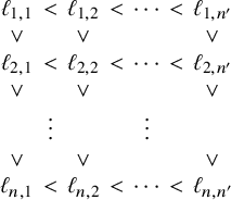
Recall the cuspidal width is defined as

$$ \begin{align*}\ell(\mu,\mu') \ = \ \min\{|\ell_{i,j}| \ : \ 1 \leq i \leq n, \ 1 \leq j \leq n'\}. \end{align*} $$

From (3.34), we see that the location of $0$ relative to these $nn'$ integers is important to determine the cuspidal width.

On how $\mu $ and $\mu '$ determine $\kappa $

Consider the j-th column of (3.34). Define $\ell _{0,j} = \infty $ (or a large positive integer), and $\ell _{n+1,j} = -\infty $ (or a large negative integer). For each $1 \leq j \leq n'$ , define $r_j$ with $0 \leq r_j \leq n$ such that

The integer $r_j$ defines the location of $0$ in the j-th column. For example, if all the $\ell _{*,j} \geq 0$ , then $r_j = n,$ and similarly, if all $\ell _{*,j} < 0$ , then $r_j = 0.$ Note that

$$ \begin{align*}0 \leq r_1 \leq r_2 \leq \cdots \leq r_{n'} \leq n. \end{align*} $$

Next, define a string of integers $s_j$ by: $s_j = r_j + j-1;$ then

$$ \begin{align*}0 \leq s_1 < s_2 < \cdots < s_{n'} \leq N-1. \end{align*} $$

Now define $\kappa = k_1 < \cdots < k_n$ by

(3.35) $$ \begin{align} \{k_1,\dots, k_n\} \ := \ \{1,2,\dots, N\} \setminus \{N-s_{n'}, N-s_{n'-1}, \dots, N-s_1\}. \end{align} $$

The inner structure of the cuspidal width - II

Suppose there are p strict inequalities in the sequence $r_1 \leq r_2 \leq \cdots \leq r_{n'}$ ; that is, we have

$$ \begin{align*}r_1 = \cdots = r_{t_1} \ < \ r_{t_1+1} = \cdots = r_{t_2} \ < \ \cdots \ = r_{t_p} < r_{t_p+1} = \cdots = r_{n'}. \end{align*} $$

Let us denote the common values thus:

(3.36) $$ \begin{align} r^{(1)} \ := \ r_1 = \cdots = r_{t_1}, \quad r^{(2)} \ := \ r_{t_1+1} = \cdots = r_{t_2}, \quad \dots, \quad r^{(p+1)} \ := \ r_{t_p+1} = \cdots = r_{n'}. \end{align} $$

Note that $1 \leq t_1 < t_2 < \cdots < t_p < n'.$ Define the quantity

(3.37) $$ \begin{align} \delta \ := \ 2(p+1) - \delta(r_1,0) - \delta(r_{n'},n), \end{align} $$

where in the last two terms, $\delta (i,j) = 1$ if $i=j$ and $\delta (i,j) =0$ if $i \neq j.$ We have the following:

Lemma 3.38. The cuspidal width $\ell (\mu ,\mu ')$ is the minimum of the set

$$ \begin{align*}{\mathbb{L}} \ := \ \{\ell_{r^{(1)},\, 1}, \ -\ell_{r^{(1)}+1, \, t_1}, \ \ell_{r^{(2)}, \, t_1+1}, \ -\ell_{r^{(2)}+1, \, t_2}, \ \dots \ \ell_{r^{(p+1)}, \, t_p+1}, \ -\ell_{r^{(p+1)}+1, \, n'} \} \end{align*} $$

with the understanding that

• ○ if $\delta (r_1,0) = 1$ , then $r^{(1)}=0$ , and we delete the term $\ell _{r^{(1)},\, 1}$ from ${\mathbb {L}}$ , and similarly,

• ○ if $\delta (r_{n'},n) = 1$ , then $r^{(p+1)} = n$ , and we delete the term $-\ell _{r^{(p+1)}+1, \, n'}$ from ${\mathbb {L}}.$

The cardinality of the set ${\mathbb {L}}$ is $\delta .$

Proof. This follows from (3.34); the cardinality of ${\mathbb {L}}$ follows from (3.37).

The proof of the combinatorial lemma - I

The proof of (2) $\iff $ (3) in Lemma 3.16 for the case of an imaginary quadratic extension follows from the following:

Proposition 3.39. The following are equivalent:

1. 1. $-N+2-\ell (\mu ,\mu ') \ \leq \ (\mathbf {{w}}-\mathbf {{w}}') \ \leq \ -N-2+\ell (\mu ,\mu ').$

2. 2. The element $w = (w_\kappa , w_{\kappa ^{\mathrm {v}}})$ satisfies $w^{-1}\cdot (\mu +\mu ')$ is dominant.

Note that the requirement of the Kostant representative to be balanced is automatically taken care of by (2), since by Lemma 3.26, (2), we have $l(w) = l(w_\kappa ) + l(w_{\kappa ^{\mathrm {v}}}) = nn'.$

Proof. The information contained in the inequalities

$$ \begin{align*}-N+2-\ell(\mu,\mu') \ \leq \ (\mathbf{{w}}-\mathbf{{w}}') \ \leq \ -N-2+\ell(\mu,\mu') \end{align*} $$

is clearly equivalent to the set of $2\delta $ inequalities

(3.40) $$ \begin{align} \ell \ \geq \ 2 + (N+(\mathbf{{w}} - \mathbf{{w}}')) \quad \mathrm{and} \quad \ell \geq 2 - (N+(\mathbf{{w}} - \mathbf{{w}}')), \quad \forall \ell \in {\mathbb{L}}. \end{align} $$

Let us begin the analysis of various cases and consider each of the above inequalities:

• ○ Suppose $r_1 = 0.$ From (3.35), it follows that $r_1 = 0 \iff k_n \leq N-1 \iff k_1^{\mathrm {v}} \geq 2.$ The condition $r_1 = \cdots = r_{t_1} = 0$ (which means the first $t_1$ many columns of (3.34) are negative) implies that $N-t_1+1,\dots , N-1, N$ are deleted in defining $\kappa $ in (3.35); hence, $k_n = N-t_1.$ Now, consider the term $\ell = -\ell _{r^{(1)}+1, \, t_1} = -\ell _{1, N-k_n} \in {\mathbb {L}}.$ From (3.33), we have

  $$ \begin{align*}-\ell_{1,N-k_n} \ = \ 2(b_n - b^{\prime}_{k_n+1-n}) - (N+(\mathbf{{w}} - \mathbf{{w}}')) + 2n' - 2(N-k_n-1). \end{align*} $$
  Applying (3.40) to $-\ell _{1,N-k_n}$ gives us
  $$ \begin{align*}b_n - b^{\prime}_{k_n+1-n} \ \geq \ n-k_n + (N+(\mathbf{{w}} - \mathbf{{w}}')), \quad \mathrm{and} \quad b_n - b^{\prime}_{k_n+1-n} \ \geq \ n-k_n, \end{align*} $$
  which are the same as the bounds in case- $(0^{\mathrm {v}})$ of Proposition 3.31 and case- $(n)$ of Proposition 3.28.

• ○ Suppose $r_{n'} = n.$ From (3.35), it follows that $r_1 = 0 \iff k_1 \geq 2 \iff k_n^{\mathrm {v}} \leq N-1.$ The condition $r_{t_p+1} = \cdots = r_{n'} = n$ (which means that in (3.34) the last $t_p$ -columns are all non-negative) implies that $1,2,\dots , N-(n+t_p)$ are deleted in getting $\kappa $ in (3.35); hence, $k_1 = n'-t_p+1.$ Now, consider the term $\ell = -\ell _{r^{(p+1)}, \, t_p +1} = -\ell _{n, n'-k_1+2} \in {\mathbb {L}}.$ From (3.33), we have

  $$ \begin{align*}\ell_{n, n'-k_1+2} \ = \ 2(b^{\prime}_{k_1-1} - b_1) + (N+(\mathbf{{w}} - \mathbf{{w}}')) - 2k_1-2n+4. \end{align*} $$
  Applying (3.40) to $\ell _{n, n'-k_1+2}$ gives us
  $$ \begin{align*}b^{\prime}_{k_1-1} - b_1 \ \geq \ n+k_1-1 , \quad \mathrm{and} \quad b^{\prime}_{k_1-1} - b_1 \ \geq \ n+k_1 -1 + (N+(\mathbf{{w}} - \mathbf{{w}}')), \end{align*} $$
  which are exactly the bounds described case- $(0)$ of Proposition 3.28 and case- $(n)^{\mathrm {v}}$ of Proposition 3.31.

• ○ Suppose $r_1 \geq 1.$ Then the shape of $\kappa $ is of the form

  $$ \begin{align*}\kappa \ = \ \{ \dots, N-r_1-t_1, \widehat{N-r_1+ - t_1}, \dots, \widehat{N - r_1}, N-r_1+1, \dots, N-1, N \}, \end{align*} $$
  where the $\widehat {a}$ means that a is deleted from that list. This implies that
  $$ \begin{align*}k_n = N, \ k_{n-1} = N-1, \ \dots, k_{n-r_1+1} = N-r_1+1, \ k_{n-r_1} = N-r_1-t_1, \dots \end{align*} $$
  Hence, we see that
  $$ \begin{align*}\mbox{if} \ l \ := \ n - r_1 \ \text{then} \ k_l = N-r_1-t_1, \ \ k_{l+1} = N-r_1+1. \end{align*} $$
  In particular, $k_{l+1} - k_l = 1+t_1 \geq 2.$ Put $l^{\mathrm {v}} = n-l+1$ . Then, by definition of $\kappa ^{\mathrm {v}}$ , we also have $k^{\mathrm {v}}_{l^{\mathrm {v}}} - k^{\mathrm {v}}_{l^{\mathrm {v}}-1} \geq 2.$ Note that $l^{\mathrm {v}} = n-(n-r_1)+1 = r_1+1.$ Hence, we have $k^{\mathrm {v}}_{r_1+1} - k^{\mathrm {v}}_{r_1} \geq 2.$ Consider the elements $\ell _{r_1, 1}$ and $-\ell _{r_1+1, t_1}$ in ${\mathbb {L}}.$ Note that
  $$ \begin{align*}\ell_{r_1,1} = 2(b^{\prime}_{n'} - b_{n-r_1+1}) + (N + (\mathbf{{w}}-\mathbf{{w}}')) - 2n' + 2(1-r_1). \end{align*} $$
  If we apply (3.40) to $\ell _{r_1,1}$ , we get
  $$ \begin{align*}b^{\prime}_{n'} - b_{n-r_1+1} \geq n'+r_1 \quad \mathrm{and} \quad b^{\prime}_{n'} - b_{n-r_1+1} \geq n'+r_1 - (N+(\mathbf{{w}}-\mathbf{{w}}')). \end{align*} $$
  We will leave it to the reader check that these are exactly the inequalities we get from case- $(l)(ii)$ of Proposition 3.28 and case- $(r_1)^{\mathrm {v}}(i)^{\mathrm {v}}$ of Proposition 3.31. Next, note that
  $$ \begin{align*}-\ell_{r_1+1, t_1} = -2(b^{\prime}_{n'-t_1+1} - b_{n-r_1}) - (N + (\mathbf{{w}}-\mathbf{{w}}')) + 2n' - 2(t_1-r_1-1). \end{align*} $$
  Apply (3.40) to $-\ell _{r_1+1, t_1}$ to get
  $$ \begin{align*}b_{n-r_1} - b^{\prime}_{n'-t_1+1} \geq -n' + t_1 - r_1 \end{align*} $$
  and
  $$ \begin{align*}b_{n-r_1} - b^{\prime}_{n'-t_1+1} \geq -n' + t_1 - r_1 + (Nr_1+(\mathbf{{w}}-\mathbf{{w}}')). \end{align*} $$
  We will leave it to the reader check that these are exactly the inequalities we get from case- $(l)(i)$ of Proposition 3.28 and case- $(r_1)^{\mathrm {v}}(ii)^{\mathrm {v}}$ of Proposition 3.31. Let us summarize the above three cases as follows:

  1. 1. If $r_1 = 0$ , then $(n)$ and $(0^{\mathrm {v}})$ hold.

  2. 2. If $r_{n'} = n$ , then $(0)$ and $(n)^{\mathrm {v}}$ hold.

  3. 3. If $r_1 \geq 1$ , then $(n-r_1)(i)$ , $(n-r_1)(ii)$ , $(r_1^{\mathrm {v}})(i)^{\mathrm {v}}$ and $(r_1^{\mathrm {v}})(ii)^{\mathrm {v}}$ hold. (Furthermore, cases $(1)^{\mathrm {v}}$ through $(r_1-1)^{\mathrm {v}}$ are empty and $(n-r_1+1)$ through $(n)$ are empty.)

• ○ It should be clear now, that for each q with $1 \leq q \leq p$ , using $t_q$ or $r^{(q)}$ as the anchor, we get all the cases of Proposition 3.28 and Proposition 3.31, and hence, $w^{-1}\cdot (\mu +\mu ')$ is dominant.

The entire argument is reversible; that is, if the cases of Proposition 3.28 and Proposition 3.31 hold, the inequalities in (3.40) are satisfied. This completes the proof of Proposition 3.39.

The general totally imaginary field

Now if F is any totally imaginary field, then the proof reduces to working with pairs of complex embeddings $(\eta _v, \bar {\eta }_v)$ for a $v \in \mathrm {S}_\infty $ ; it is entirely analogous to Section 3.2.3. We will leave the details to the reader.

3.2.5 The combinatorial lemma at an arithmetic level

All the three statements in Lemma 3.16 work at an arithmetic level. Take $\mu \in X^+_{00}(T_n \times E)$ and $\mu ' \in X^+_{00}(T_{n'} \times E)$ , and $\sigma _f \in \mathrm {{Coh}}_{!!}(G_n, \mu )$ , $\sigma ^{\prime }_f \in \mathrm {{Coh}}_{!!}(G_{n'}, \mu '),$ and for $\iota : E \to \mathbb {C}$ , consider the statement of the lemma for ${}^\iota \mu , {}^\iota \mu ', {}^\iota \sigma $ and ${}^\iota \sigma '$ ; let us add some comments for each of (1), (2) and (3) of the lemma:

1. 1. From Section 3.1.3, it follows that $-\tfrac {N}{2}$ and $1-\tfrac {N}{2}$ are critical for $L(s, {}^\iota \sigma \times {}^\iota \sigma ^{\prime \mathrm {v}})$ for any $\iota : E \to \mathbb {C}.$

2. 2. Since $\mu $ and $\mu '$ are strongly-pure, it is easy to see that the abelian width $a({}^\iota \mu , {}^\iota \mu ')$ and the cuspidal width $\ell ({}^\iota \mu , {}^\iota \mu ')$ are independent of $\iota .$ (See Corollary 3.15.) For the assertion for cuspidal width, the reader may check from definitions that the $\ell ({}^\iota \mu , {}^\iota \mu ')$ is given by taking the minimum of $|-2\mu ^{\iota \circ \tau }_{n-i+1}+2\mu ^{\prime \iota \circ \tau }_{n'-j+1} + n-n' + 2j-2i + \mathbf {{w}} -\mathbf {{w}}'|$ over all $\tau : F \to E,$ and all indices $1 \leq i \leq n, \ 1 \leq j \leq n'.$ As $\tau $ varies over $\mathrm {{Hom}}(F,E)$ , $\iota \circ \tau $ varies over $\mathrm {{Hom}}(F,\mathbb {C}),$ making the above minimum independent of $\iota .$

3. 3. Write $w \in W^G$ as $w = (w^\tau )_{\tau : F \to E}.$ We will say $w \in W^P$ is balanced if $l(w^\tau ) + l(w^{\overline {\tau }^\iota }) = \dim (U_{P_0})$ for all $\tau \in \mathrm {{Hom}}(F,E)$ and for all $\iota : E \to \mathbb {C}$ ; recall that $\iota $ induces a complex conjugation $\tau \mapsto {\overline {\tau }^\iota }$ on $\mathrm {{Hom}}(F,E)$ . (See Remark 3.41 below.)

It should now be clear that $(1) \iff (2) \iff (3)$ of the lemma is independent of $\iota : E \to \mathbb {C}.$

Remark 3.41. Strongly-pure weights $\mu \in X^+_{00}(T_n \times E)$ and $\mu ' \in X^+_{00}(T_{n'} \times E)$ being the base-change from $F_1$ (Proposition 2.6), it follows when the conditions of the combinatorial lemma (Lemma 3.16) hold, that the Kostant representative $w = (w^\tau )_{\tau : F \to E}$ is also the base-change from $F_1$ in the sense that if $\tau |_{F_1} = \tau '|_{F_1}$ , then $w^{\tau } = w^{\tau '}.$

4 Archimedean intertwining operator

As mentioned in the Introduction, typically, in a cohomological approach to the study of the special values of L-functions, one is confronted with an archimedean subproblem which is taken up in this section. The problem is to compute the map induced in relative Lie algebra cohomology by the archimedean standard intertwining operator $T_\infty $ between two irreducible modules, and show that for optimally chosen bases for these cohomology groups, this map is essentially scaling by the appropriate ratio of archimedean L-factors. In 4.1, we go through the $\mathrm {{GL}}(2)$ -calculation which culminates in Proposition 4.20, which is then used in its generalization in Proposition 4.32, which is the main result of this section. For a first reading, it is suggested to understand and assume the statements of these two propositions and come back to their proofs at a later point of time.

4.1 The case of $\mathrm {{GL}}_2$

The calculations in this subsection are in principle the same as in Harder [22, Sect. 3.5], but we need to go through this exercise to reorganise our thoughts, while using inputs from [27, Chap. 9], so as to generalize them to $\mathrm {{GL}}_N$ in the next subsection. The main result of this subsection is Proposition 4.20.

4.1.1 Explicit cohomology class for $\mathrm {{GL}}_2$

Let $\mu = ((b_1,b_2), (c_1,c_2))$ be a pure dominant integral weight for $\mathrm {{GL}}_2(\mathbb {C})$ as a real group. Integrality means $b_1,b_2,c_1,c_2 \in \mathbb {Z}$ ; dominance is $b_1 \geq b_2$ and $c_1 \geq c_2$ ; purity means $b_1+c_2 = b_2+c_1$ , which allows us to define $m := b_1-b_2 +1 = c_1-c_2+1$ . The cuspidal parameters are $(\alpha _1,\alpha _2) = (-b_2+ \tfrac 12,-b_1-\tfrac 12)$ and $(\beta _1,\beta _2) = (-c_1-\tfrac 12, -c_2+\tfrac 12).$ We have the induced representation

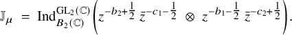$$ \begin{align*}\mathbb{J}_\mu \ = \ \mathrm{{Ind}}_{B_2(\mathbb{C})}^{\mathrm{{GL}}_2(\mathbb{C})}\left( z^{-b_2+ \tfrac12} \, \bar{z}^{-c_1-\tfrac12} \ \otimes \ z^{-b_1-\tfrac12} \, \bar{z}^{-c_2+\tfrac12} \right). \end{align*} $$

Recall $\mathrm {{GL}}_2(\mathbb {C}) = B_2(\mathbb {C}) \mathrm {{SU}}(2)$ with $T_c^{(1)} := B_2(\mathbb {C}) \cap \mathrm {{SU}}(2) \approx \mathrm {{SU}}(1) \approx \mathbf {{S}}^1.$ Let us write $e^{i\theta }$ for an element of $\mathbf {{S}}^1$ which is the element $\left (\begin {smallmatrix} e^{i\theta } & 0 \\ 0 & e^{-i\theta }\end {smallmatrix}\right )$ in $T_c^{(1)}$ . If $(\tau _k,V_k)$ denotes the irreducible representation of $\mathrm {{SU}}(2)$ of dimension k, and $\chi _{2m}(e^{i \theta }) = e^{i (2m)\theta },$ then

(4.1) $$ \begin{align} \mathbb{J}_\mu \ = \ \mathrm{{Ind}}_{T_c^{(1)}}^{\mathrm{{SU}}(2)} \left(\chi_{2m}\right) \ \approx \ \tau_{2m+1} \oplus \tau_{2m+3} \oplus \cdots \oplus \tau_{2m+2k+1} \oplus \cdots, \end{align} $$

since by Frobenius reciprocity, any irreducible representation of $\mathrm {{SU}}(2)$ that appears in $\mathbb {J}_\mu $ has to contain the character $\chi _{2m}$ with multiplicity one. Note that $\tau _{2m+1}$ is the minimal K-type in the induced representation $\mathbb {J}_\mu ;$ we denote $\mathbb {J}_\mu (\tau _{2m+1})$ for this minimal K-type as it sits inside the ambient $\mathbb {J}_\mu $ . Let us next describe $(\rho _\mu ,\mathcal {M}_\mu )$ restricted to $\mathrm {{SU}}(2).$ We have $\mathcal {M}_{(b_1,b_2)} = \text {Sym}^{b_1-b_2}(\mathbb {C}^2) \otimes \det ^{b_2}$ as a representation of $\mathrm {{GL}}_2(\mathbb {C}),$ where $\mathbb {C}^2$ is the standard representation. Hence, $\rho _{(b_1,b_2)}|_{\mathrm {{SU}}(2)} = \tau _m.$ Similarly, ${\rho _{(c_1,c_2)}|_{\mathrm {{SU}}(2)} = \tau _m.}$ If $g \in \mathrm {{SU}}(2)$ , then $\bar {g} = {}^t g^{-1}$ ; hence, $\bar {\tau }_m = \tau _m^\vee = \tau _m.$ This implies that $\rho _\mu |_{\mathrm {{SU}}(2)} = \tau _m \otimes \tau _m.$ Recall Clebsch-Gordon for $\mathrm {{SU}}(2)$ : for $p \geq q \geq 1$ , we have

(4.2) $$ \begin{align} \tau_p \otimes \tau_q \ = \ \tau_{p-q+1} \oplus \tau_{p-q+3} \oplus \cdots \oplus \tau_{p+q-1}. \end{align} $$

Applying this to $p = q = m$ we get

(4.3) $$ \begin{align} \rho_\mu|_{\mathrm{{SU}}(2)} \ = \ \tau_1 \oplus \tau_3 \oplus \cdots \oplus \tau_{2m-1}. \end{align} $$

Denote $\mathcal {M}_\mu (\tau _{2m-1})$ for the copy of $\tau _{2m-1}$ as it sits inside $\mathcal {M}_\mu .$ Let $\mathfrak {g}_2 := \mathfrak {gl}_2(\mathbb {C})$ and $\tilde {\mathfrak {k}}_2 := \mathbb {R} \oplus {\mathfrak {u}}_2(\mathbb {C})$ be the Lie algebras of the connected real Lie groups $\mathrm {{GL}}_2(\mathbb {C})$ and $Z_2(\mathbb {C})\mathrm {{U}}(2),$ respectively. Then the Adjoint-action of $\mathrm {{SU}}(2)$ on $\mathfrak {g}_2/\tilde {\mathfrak {k}}_2$ is irreducible whose complexification is isomorphic to $\tau _3.$ Furthermore, we have $\wedge ^0(\mathfrak {g}_2/\tilde {\mathfrak {k}}_2) \approx \wedge ^3(\mathfrak {g}_2/\tilde {\mathfrak {k}}_2) \approx \tau _1$ and $\wedge ^1(\mathfrak {g}_2/\tilde {\mathfrak {k}}_2) \approx \wedge ^2(\mathfrak {g}_2/\tilde {\mathfrak {k}}_2) \approx \tau _3.$ We can now describe the complex $\mathrm {{Hom}}_{\mathrm {{SU}}(2)}(\wedge ^{\bullet }(\mathfrak {g}_2/\tilde {\mathfrak {k}}_2), \mathbb {J}_\mu \otimes \mathcal {M}_\mu ).$ Apply (4.1) and (4.3) to $\mathbb {J}_\mu \otimes \mathcal {M}_\mu $ and then apply (4.2) to see that the smallest p for which $\tau _p$ can occur in $\mathbb {J}_\mu \otimes \mathcal {M}_\mu $ is $p=3$ and this is realized exactly once as

$$ \begin{align*}\tau_3 \ \hookrightarrow \ \tau_{2m+1} \otimes \tau_{2m-1} \ = \ \mathbb{J}_\mu(\tau_{2m+1}) \otimes \mathcal{M}_\mu(\tau_{2m-1}). \end{align*} $$

Hence, $\mathrm {{Hom}}_{\mathrm {{SU}}(2)}(\wedge ^{\bullet }(\mathfrak {g}_2/\tilde {\mathfrak {k}}_2), \mathbb {J}_\mu \otimes \mathcal {M}_\mu ) \neq 0 \iff \bullet = 1, 2,$ and is one-dimensional in these degrees. Knowing that the differentials for this complex are zero, we deduce that $\mathbb {J}_\mu \otimes \mathcal {M}_\mu $ has nonvanishing $(\mathfrak {g}_2, \tilde {\mathfrak {k}}_2)$ -cohomology only in degrees $1$ and $2$ and the cohomology group is one-dimensional in these degrees. Fix a basis $[\mathbb {J}_\mu ]$ for

(4.4) $$ \begin{align} H^1(\mathfrak{g}_2, \tilde{{\mathfrak{k}}}_2; \mathbb{J}_\mu \otimes \mathcal{M}_\mu) \ = \ H^1(\mathfrak{gl}_2(\mathbb{C}), Z_2(\mathbb{C})\mathrm{{U}}(2); \mathbb{J}_\mu \otimes \mathcal{M}_\mu) \ = \ \mathbb{C} [\mathbb{J}_\mu]. \end{align} $$

Now, we express $[\mathbb {J}_\mu ] \in \mathrm {{Hom}}_{Z_2(\mathbb {C})\mathrm {{U}}(2)}(1\!\!1, \wedge ^1(\mathfrak {g}_2/\tilde {\mathfrak {k}}_2)^{*} \otimes \mathbb {J}_\mu (\tau _{2m+1}) \otimes \mathcal {M}_\mu (\tau _{2m-1})),$ as

$$ \begin{align*}[\mathbb{J}_\mu] \ = \ \sum_{i, \alpha} X_i^{*} \otimes \phi_{i, \alpha} \otimes m_{\alpha}, \end{align*} $$

where $\{X_i^{*}\}$ is a basis for $(\mathfrak {g}_2/\tilde {\mathfrak {k}}_2)^{*}$ , and $\{m_\alpha \}$ is a basis for $\mathcal {M}_\mu .$ (Of course, if $m_\alpha \notin \mathcal {M}_\mu (\tau _{2m-1})$ , then $\phi _{i, \alpha } = 0.$ ) We call the finite set $\{\phi _{i, \alpha }\}$ of vectors in $\mathbb {J}_\mu $ as cohomological vectors. Since $H^1$ has dimension one, a scaling of the basis element $[\mathbb {J}_\mu ]$ means jointly scaling this finite set of cohomological vectors. Furthermore, we contend, via an explicit version of Clebsch–Gordon, that one of the $\phi _{i, \alpha }$ is a highest weight vector of the lowest K-type $\mathbb {J}_\mu (\tau _{2m+1}).$ Call this particular vector as the distinguished cohomological vector for a given choice of $[\mathbb {J}_\mu ]$ .

4.1.2 The highest weight vector of the lowest K-type in $\mathbb {J}_\mu $

We can explicitly describe such a vector $f_\mu $ ; first of all, since $f_\mu $ is in the induced representation $\mathbb {J}_\mu $ we have

(4.5) $$ \begin{align} f_\mu\left(\begin{pmatrix}z & * \\ & w \end{pmatrix} g\right) \ = \ z^{-b_2+ \tfrac12} \, \bar{z}^{-c_1-\tfrac12} \cdot w^{-b_1-\tfrac12} \, \bar{w}^{-c_2+\tfrac12} \cdot \left|\frac{z}{w}\right|{}_{\mathbb{C}}^{1/2} f_\mu(g), \end{align} $$

for all $g \in \mathrm {{GL}}_2(\mathbb {C})$ and $z,w\in \mathbb {C}^{\times }.$ Next, we note

(4.6) $$ \begin{align} f_\mu \left( \begin{pmatrix} e^{i\alpha} & \\ & e^{-i\alpha} \end{pmatrix} g \begin{pmatrix} e^{i\beta} & \\ & e^{-i\beta} \end{pmatrix}\right) = \ e^{i(2m)\alpha} e^{i(2m)\beta} f_\mu(g), \end{align} $$

for all $g \in \mathrm {{GL}}_2(\mathbb {C})$ . The left-equivariance under $T_c^{(1)}$ is by (4.5), and the right-equivariance under $T_c^{(1)}$ is because of being the highest weight vector in $\tau _{2m+1}$ . Finally, $f_\mu $ is completely determined by its values on $\mathrm {{SU}}(2)$ , for which, observe that $\mathrm {{SU}}(2) = T_c^{(1)} \cdot \mathrm {{SO}}(2) \cdot T_c^{(1)}.$ For the values of $f_\mu $ on $\mathrm {{SO}}(2)$ , recall that the weight-vectors of $\tau _{2m+1}$ maybe enumerated as $\{f_{-2m}, f_{-2m+2}, \dots , f_{2m-2}, f_{2m}\}$ , where $T_c^{(1)}$ acts on $f_k$ via the character $e^{i \beta } \mapsto e^{ik\beta }.$ So our $f_\mu $ is $f_{2m}$ up to a scalar multiple. Let ${\mathfrak {r}}(\theta ) = \left (\begin {smallmatrix} \cos (\theta ) & -\sin (\theta ) \\ \sin (\theta ) & \cos (\theta ) \end {smallmatrix}\right )$ ; then the weight vectors $\{f_{-2m}, f_{-2m+2}, \dots , f_{2m-2}\}$ may be normalized so that

(4.7) $$ \begin{align} {\mathfrak{r}}(\theta) \cdot f_{2m} \ = \ \cos^{2m}(\theta)f_{2m} \ + \ \cos^{2m-2}(\theta)\sin^2(\theta) f_{2m-2} \ + \ \cdots \ + \ \sin^{2m}(\theta)f_{-2m}. \end{align} $$

(Think of the model for $\tau _{2m+1}$ consisting of homogeneous polynomials of degree $2m$ in two variables.) Using the analogue of (4.6) for the other weight vectors, we see that $f_k(I) = 0$ if $k \neq 2m$ . (Here, I is the $2 \times 2$ identity matrix.) Evaluating (4.7) on I, we get

(4.8) $$ \begin{align} f_\mu({\mathfrak{r}}(\theta)) \ = \ \cos^{2m}(\theta), \end{align} $$

where we have normalized $f_\mu $ by $f_{\mu }(I) = 1.$ Putting (4.5), (4.6) and (4.8) together, we can write

(4.9) $$ \begin{align} f_\mu \left(\begin{pmatrix}z & * \\ & w \end{pmatrix} {\mathfrak{r}}(\theta) \begin{pmatrix} e^{i\beta} & \\ & e^{-i\beta} \end{pmatrix} \right) \ = \ z^{-b_2+ 1} \, \bar{z}^{-c_1} \cdot w^{-b_1-1} \bar{w}^{-c_2} \cdot \cos^{2m}(\theta) \cdot e^{i(2m)\beta}. \end{align} $$

4.1.3 The cohomology class $[\mathbb {J}_\mu ]_0$

The compact Lie group $\mathrm {{SO}}(2)$ is the real points of an algebraic group defined over $\mathbb {Q}$ , whose $\mathbb {Q}$ -points we denote $\mathrm {{SO}}(2)(\mathbb {Q})$ ; this consists of all those ${\mathfrak {r}}(\theta )$ such that $\cos (\theta ), \, \sin (\theta ) \in \mathbb {Q}$ . We will scale the cohomology class $[\mathbb {J}_\mu ]$ , such that the distinguished cohomological vector is rational – that is, takes rational values on $\mathrm {{SO}}(2)(\mathbb {Q});$ we denote this class by $[\mathbb {J}_\mu ]_0$ . Observe that $[\mathbb {J}_\mu ]_0$ is well defined only up to homothety by $\mathbb {Q}^{\times }.$ By (4.9), we see that some $\mathbb {Q}^{\times }$ -multiple of $f_\mu $ is a distinguished cohomological vector for $[\mathbb {J}_\mu ]_0.$

4.1.4 The intertwining operator $T_{\mathrm {st}}$

Consider the induced representation

$$ \begin{align*}\mathbb{J}_\mu \ = \ \mathrm{{Ind}}_{B_2(\mathbb{C})}^{\mathrm{{GL}}_2(\mathbb{C})}\left( z^{-b_2+ \tfrac12} \, \bar{z}^{-c_1-\tfrac12} \ \otimes \ z^{-b_1-\tfrac12} \, \bar{z}^{-c_2+\tfrac12} \right) \ \ \mathrm{as} \ \ \mathrm{{Ind}}_{B_2(\mathbb{C})}^{\mathrm{{GL}}_2(\mathbb{C})}(\chi_1(\mu) \otimes \chi_2(\mu)), \end{align*} $$

where $\chi _1(\mu )(z) = z^{-b_2+ \tfrac 12} \, \bar {z}^{-c_1-\tfrac 12}$ and $\chi _2(\mu )(z) = z^{-b_1-\tfrac 12} \, \bar {z}^{-c_2+\tfrac 12}.$ The standard intertwining operator from $\mathbb {J}_\mu $ to its ‘companion’ induced representation

$$ \begin{align*}T_{\mathrm{st}} : \mathrm{{Ind}}_{B_2(\mathbb{C})}^{\mathrm{{GL}}_2(\mathbb{C})}(\chi_1(\mu) \otimes \chi_2(\mu)) \ \longrightarrow \ \mathrm{{Ind}}_{B_2(\mathbb{C})}^{\mathrm{{GL}}_2(\mathbb{C})}(\chi_2(\mu) \otimes \chi_1(\mu)) \end{align*} $$

is given by the integral

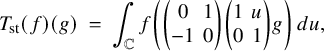(4.10) $$ \begin{align} T_{\mathrm{st}}(f)(g) \ = \ \int_{\mathbb{C}} f \left( \begin{pmatrix} 0 & 1 \\ -1 & 0 \end{pmatrix} \begin{pmatrix} 1 & u \\ 0 & 1 \end{pmatrix} g \right) \, du, \end{align} $$

where $du$ is the Lebesgue measure on $\mathbb {C}$ ; if $u = x + {\mathfrak {i}} y$ then $du = dx\,dy.$

Proposition 4.11. Suppose $s = -1$ and $s=0$ are regular points for both $L(s, \chi _1(\mu )\chi _2(\mu )^{-1})$ and $L(1-s, \chi _1(\mu )^{-1}\chi _2(\mu )).$ Then, the representation $\mathrm {{Ind}}_{B_2(\mathbb {C})}^{\mathrm {{GL}}_2(\mathbb {C})}(\chi _1(\mu ) \otimes \chi _2(\mu ))$ is irreducible, and the standard intertwining operator $T_{\mathrm {st}}$ is an isomorphism.

Proof. Irreducibility follows from [20, Chap. 2, Thm. 3]. The proof of $T_{\mathrm { st}}$ being an isomorphism follows the same argument as in the proof of [27, Prop. 7.54]. We will elaborate further when we deal with $\mathrm {{GL}}_N$ ; see Proposition 4.28 below.

4.1.5 The highest weight vector of the lowest K-type on the ‘other side’

Since $T_{\mathrm {st}}$ is an isomorphism of $\mathrm {{GL}}_2(\mathbb {C})$ -modules, it maps the minimal $\mathrm {{SU}}(2)$ -type in $\mathrm {{Ind}}(\chi _1(\mu ) \otimes \chi _2(\mu ))$ isomorphically onto the minimal $\mathrm {{SU}}(2)$ -type in $\mathrm {{Ind}}(\chi _2(\mu ) \otimes \chi _1(\mu ))$ , and within these $\mathrm {{SU}}(2)$ -types, it maps $f_\mu $ , which is the highest weight vector for $T_c^{(1)}$ described above to a multiple of the highest weight vector on the other side, which we denote $\tilde {f_\mu }$ . We have the analogues of (4.5) and (4.6) for $\tilde {f_\mu }$ :

(4.12) $$ \begin{align} \tilde f_\mu \left(\begin{pmatrix}z & * \\ & w \end{pmatrix} g \right) \ = \ z^{-b_1-\tfrac12} \, \bar{z}^{-c_2+\tfrac12} \cdot w^{-b_2+ \tfrac12} \, \bar{w}^{-c_1-\tfrac12} \cdot \left|\frac{z}{w}\right|{}_{\mathbb{C}}^{1/2} \tilde f_\mu(g), \end{align} $$

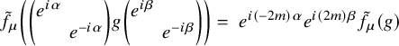(4.13) $$ \begin{align} \tilde f_\mu \left( \begin{pmatrix} e^{i\alpha} & \\ & e^{-i\alpha} \end{pmatrix} g \begin{pmatrix} e^{i\beta} & \\ & e^{-i\beta} \end{pmatrix} \right) = \ e^{i(-2m)\alpha} e^{i(2m)\beta} \tilde f_\mu(g) \end{align} $$

for all $g \in \mathrm {{GL}}_2(\mathbb {C}).$ But, (4.13) also says that $\tilde f_\mu (I) = 0$ (since $m \geq 1$ ). Let $w_0 = \left (\begin {smallmatrix} 0 & 1 \\ -1 & 0 \end {smallmatrix}\right ) \ = \ {\mathfrak {r}}(-\pi /2).$ Then, using (4.7), and evaluating at $w_0$ we see $({\mathfrak {r}}(\theta )\cdot \tilde f_\mu )(w_0) = \cos ^{2m}(\theta ) \cdot \tilde f_\mu (w_0).$ (The other summands vanish on $w_0$ using the analogue of (4.13).) Hence,

$$ \begin{align*}\tilde f_\mu({\mathfrak{r}}(\theta - \pi/2)) \ = \ \tilde f_\mu (w_0 {\mathfrak{r}}(\theta)) \ = \ \cos^{2m}(\theta) \cdot \tilde f_\mu(w_0). \end{align*} $$

Change $\theta \mapsto \theta +\pi /2$ , and noting $\cos (\theta +\pi /2) = - \sin (\theta )$ , we get the analogue of (4.8):

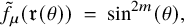(4.14) $$ \begin{align} \tilde f_\mu({\mathfrak{r}}(\theta)) \ = \ \sin^{2m}(\theta), \end{align} $$

where we have normalized $\tilde f_\mu $ by $\tilde f_{\mu }(w_0) = 1.$ From (4.12), (4.13) and (4.14), we have

(4.15) $$ \begin{align} \tilde f_\mu \left(\begin{pmatrix}z & * \\ & w \end{pmatrix} {\mathfrak{r}}(\theta) \begin{pmatrix} e^{i\beta} & \\ & e^{-i\beta} \end{pmatrix} \right) \ = \ z^{-b_1} \, \bar{z}^{-c_2+1} \cdot w^{-b_2} \bar{w}^{-c_1-1} \cdot \sin^{2m}(\theta) \cdot e^{i(2m)\beta}. \end{align} $$

4.1.6 The basic intertwining calculation for $\mathrm {{GL}}_2$

Proposition 4.16.

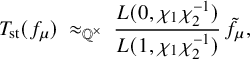$$ \begin{align*}T_{\mathrm{st}}(f_\mu) \ \approx_{\mathbb{Q}^{\times}} \ \frac{L(0, \chi_1 \chi_2^{-1})}{L(1, \chi_1 \chi_2^{-1})} \, \tilde f_\mu, \end{align*} $$

where, $\approx _{\mathbb {Q}^{\times }}$ means equality up to a nonzero rational number.

Proof. It is clear that $T_{\mathrm {st}}(f_\mu )$ is a scalar multiple of $\tilde f_\mu .$ To compute that scalar, we evaluate $T_{\mathrm {st}}(f_\mu )$ at $w_0$ :

$$ \begin{align*}T_{\mathrm{st}}(f_\mu)(w_0) \ = \ \int_{\mathbb{C}} f_\mu \left( \begin{pmatrix} 0 & 1 \\ -1 & 0 \end{pmatrix} \begin{pmatrix} 1 & u \\ 0 & 1 \end{pmatrix} \begin{pmatrix} 0 & 1 \\ -1 & 0 \end{pmatrix} \right) \, du \ = \ \int_{\mathbb{C}} f_\mu \left( \begin{pmatrix} 1 & 0 \\ -u & 1 \end{pmatrix} \right) \, du. \end{align*} $$

Change to polar coordinates: $u = r e^{i\theta }.$ Note that

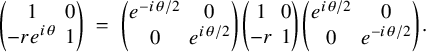$$ \begin{align*}\begin{pmatrix} 1 & 0 \\ -r e^{i\theta} & 1 \end{pmatrix} \ = \ \begin{pmatrix} e^{-i \theta/2} & 0 \\ 0 & e^{i \theta/2} \end{pmatrix} \begin{pmatrix} 1 & 0 \\ -r & 1 \end{pmatrix} \begin{pmatrix} e^{i \theta/2} & 0 \\ 0 & e^{-i \theta/2} \end{pmatrix}. \end{align*} $$

Hence, applying (4.5) and (4.6), we get

$$ \begin{align*}f_\mu \left( \begin{pmatrix} 1 & 0 \\ - r e^{i\theta}& 1 \end{pmatrix} \right) \ = \ e^{-i(2m) \theta/2} f_\mu \left(\begin{pmatrix} 1 & 0 \\ - r & 1 \end{pmatrix}\right) e^{i(2m) \theta/2} \ = \ f_\mu \left(\begin{pmatrix} 1 & 0 \\ - r & 1 \end{pmatrix}\right). \end{align*} $$

Next, we note

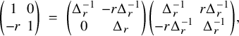$$ \begin{align*}\begin{pmatrix} 1 & 0 \\ - r & 1 \end{pmatrix} \ = \ \begin{pmatrix} \Delta_r^{-1} & -r\Delta_r^{-1} \\ 0 & \Delta_r \end{pmatrix} \begin{pmatrix} \Delta_r^{-1} & r\Delta_r^{-1} \\ - r\Delta_r^{-1} & \Delta_r^{-1} \end{pmatrix}, \end{align*} $$

where $\Delta _r = \sqrt {1+r^2}.$ Note that $\left (\begin {smallmatrix} \Delta _r^{-1} & r\Delta _r^{-1} \\ - r\Delta _r^{-1} & \Delta _r^{-1} \end {smallmatrix}\right ) = {\mathfrak {r}}(\alpha )$ with $\alpha = \tan ^{-1}(-r).$ From (4.5) and (4.8), we get

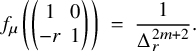$$ \begin{align*}f_\mu \left(\begin{pmatrix} 1 & 0 \\ - r & 1 \end{pmatrix}\right) \ = \ \frac{1}{\Delta_r^{2m+2}}. \end{align*} $$

The integral evaluates to

(4.17) $$ \begin{align} T_{\mathrm{st}}(f_\mu)(w_0) \ = \ \int_{\theta = 0}^{2\pi} \int_{r=0}^\infty \frac{r \, dr\, d\theta}{(\sqrt{1+r^2})^{2m+2}} \ = \ \frac{\pi}{m}. \end{align} $$

Now, $\chi _1\chi _2^{-1}(z) = z^m \bar {z}^{-m}$ , and by (3.3), we have $L(s, \chi _1\chi _2^{-1}) = 2 (2\pi )^{-(s+m)} \Gamma (s+m).$ The hypothesis in Proposition 4.11 about $s = -1$ and $s=0$ being critical implies that $m \geq 2.$

Hence,

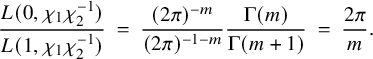(4.18) $$ \begin{align} \frac{L(0, \chi_1 \chi_2^{-1})}{L(1, \chi_1 \chi_2^{-1})} \ = \ \frac{(2\pi)^{- m}}{(2\pi)^{-1-m}} \frac{\Gamma(m)}{\Gamma(m+1)} \ = \ \frac{2\pi}{m}. \end{align} $$

The proof follows from (4.17) and (4.18).

4.1.7 Arithmetic interpretation of the intertwining calculation

Denote the induced representation in the range of $T_{\mathrm {st}}$ as $\tilde {\mathbb {J}}_\mu = \mathrm {{Ind}}(\chi _2(\mu ) \otimes \chi _1(\mu ))$ Now, fix a cohomology class $[\tilde {\mathbb {J}}_\mu ]_0$ :

(4.19) $$ \begin{align} H^1(\mathfrak{g}_2, \tilde{{\mathfrak{k}}}_2; \tilde{\mathbb{J}}_\mu \otimes \mathcal{M}_\mu) \ = \ H^1(\mathfrak{gl}_2(\mathbb{C}), Z_2(\mathbb{C})\mathrm{{U}}(2); \tilde{\mathbb{J}}_\mu \otimes \mathcal{M}_\mu) \ = \ \mathbb{C} [\tilde{\mathbb{J}}_\mu]_0, \end{align} $$

characterised by the property that its distingusihed cohomological vector is rational; hence, up to $\mathbb {Q}^{\times }$ -multiples, the vector $\tilde f_\mu $ is a cohomological vector for $\tilde {\mathbb {J}}_\mu .$ Consider the map induced in cohomology by the operator $T_{\mathrm {st}} : \mathbb {J}_\mu \to \tilde {\mathbb {J}}_\mu $ ; at the level of generators, it will map $[\mathbb {J}_\mu ] = \sum _{i, \alpha } X_i^{*} \otimes \phi _{i, \alpha } \otimes m_{\alpha }$ to $\sum _{i, \alpha } X_i^{*} \otimes T_{\mathrm {st}}(\phi _{i, \alpha }) \otimes m_{\alpha }.$ Then, in terms of the cohomology classes with rational distinguished cohomological vectors, Proposition 4.16 may be stated as

Proposition 4.20.

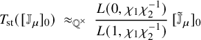$$ \begin{align*}T_{\mathrm{st}}([\mathbb{J}_\mu]_0) \ \approx_{\mathbb{Q}^{\times}} \ \frac{L(0, \chi_1 \chi_2^{-1})}{L(1, \chi_1 \chi_2^{-1})} \, [\tilde{\mathbb{J}}_\mu]_0 \end{align*} $$

Remark 4.21. Since $\chi _1\chi _2^{-1}(z) = z^m \bar {z}^{-m}$ , note that $L(0, \chi _1 \chi _2^{-1})/L(1, \chi _1 \chi _2^{-1}) \approx _{\mathbb {Q}^{\times }} \pi $ , and similarly, $L(-1, \chi _1 \chi _2^{-1})/L(0, \chi _1 \chi _2^{-1}) \approx _{\mathbb {Q}^{\times }} \pi $ . We may also state the proposition as

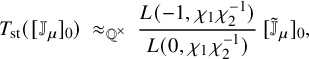$$ \begin{align*}T_{\mathrm{st}}([\mathbb{J}_\mu]_0) \ \approx_{\mathbb{Q}^{\times}} \ \frac{L(-1, \chi_1 \chi_2^{-1})}{L(0, \chi_1 \chi_2^{-1})} \, [\tilde{\mathbb{J}}_\mu]_0, \end{align*} $$

which would be the precise form in which it will generalize to Proposition 4.32.

4.1.8 Rational classes via Delorme’s Lemma

Recall Delorme’s Lemma (see Borel–Wallach [5, Thm. III.3.3]), which in the current context can be explicated as

(4.22) $$ \begin{align} &H^1(\mathfrak{g}_2, \tilde{{\mathfrak{k}}}_2; \mathbb{J}_\mu \otimes \mathcal{M}_\mu) \ \simeq \notag\\ &\qquad\qquad\quad H^0(\mathfrak{g}_1, {\mathfrak{k}}_1; z^{-b_2+1} \bar{z}^{-c_1} \otimes \mathcal{M}_{(b_2-1)(c_1)}) \otimes H^0(\mathfrak{g}_1, {\mathfrak{k}}_1; z^{-b_1-1} \bar{z}^{-c_2} \otimes \mathcal{M}_{(b_1+1)(c_2)}), \end{align} $$

where $\mathfrak {g}_1 = \mathfrak {gl}_1(\mathbb {C})$ , ${\mathfrak {k}}_1 = \mathfrak {su}(1),$ for $b, c \in \mathbb {Z}$ we abbreviate the character $z \mapsto z^{b} \bar {z}^{c}$ simply as $z^{b} \bar {z}^{c}$ , and $\mathcal {M}_{(b)(c)}$ is the algebraic representation $z^{b} \bar {z}^{c}$ of the real group $\mathbb {C}^{\times }.$ Note that on the right-hand side, in each factor, we are looking at the relative Lie algebra cohomology for $\mathrm {{GL}}_1(\mathbb {C})$ of $z^{-b} \bar {z}^{-c} \otimes \mathcal {M}_{(b)(c)},$ which is nothing but the trivial character! For brevity, denote $H^0_{b,c} = H^0(\mathfrak {g}_1, {\mathfrak {k}}_1; z^{-b} \bar {z}^{-c} \otimes \mathcal {M}_{(b)(c)}).$ Parse the isomorphism in Delorme’s Lemma: the map $f \mapsto f(1_2)$ for $f \in \mathbb {J}_\mu $ induces an isomorphism coming from Frobenius reciprocity:

$$ \begin{align*} H^1(\mathfrak{g}_2, \tilde{{\mathfrak{k}}}_2; {{}^{\mathrm{a}}\mathrm{Ind}}(z^{-b_2+1} \bar{z}^{-c_1} \otimes z^{-b_1-1} \bar{z}^{-c_2}) \otimes \mathcal{M}_\mu) \ &\simeq \\ & \ H^1({\mathfrak{b}}_2, {\mathfrak{k}}_{B_2}; (z^{-b_2+1} \bar{z}^{-c_1} \otimes z^{-b_1-1} \bar{z}^{-c_2}) \otimes \mathcal{M}_\mu), \end{align*} $$

where ${\mathfrak {b}}_2$ (resp., ${\mathfrak {k}}_{B_2}$ ) is the real Lie algebra of $B_2(\mathbb {C})$ (resp., $\mathrm {{U}}(2) \cap B_2(\mathbb {C})$ ). The proof of [5, Thm. III.3.3] gives that

$$ \begin{align*} &H^1({\mathfrak{b}}_2, {\mathfrak{k}}_B; (z^{-b_2+1} \bar{z}^{-c_1} \otimes z^{-b_1-1} \bar{z}^{-c_2}) \otimes \mathcal{M}_\mu) \ \simeq \\ &\qquad\qquad\qquad\qquad\qquad\qquad\qquad H^0({\mathfrak{t}}_2, {\mathfrak{k}}_{T_2}; (z^{-b_2+1} \bar{z}^{-c_1} \otimes z^{-b_1-1} \bar{z}^{-c_2}) \otimes H^1({\mathfrak{u}}_{B_2}, \mathcal{M}_\mu)), \end{align*} $$

where ${\mathfrak {t}}_2$ , ${\mathfrak {k}}_{T_2}$ and ${\mathfrak {u}}_{B_2}$ are the real Lie algebras of the diagonal torus $T_2(\mathbb {C})$ in $B_2(\mathbb {C})$ , its maximal compact $\mathrm {{U}}(2) \cap T_2(\mathbb {C})$ , and the unipotent radical of $B_2(\mathbb {C})$ , respectively. To apply Kostant’s theorem (2.24), we need the Kostant representatives of length $1$ for the Borel subgroup in the real reductive group $\mathrm {{GL}}_2(\mathbb {C});$ if $w_0 = \left (\begin {smallmatrix} 0 & 1 \\ -1 & 0 \end {smallmatrix}\right )$ , then therequired Kostant representatives are $w_l = (w_0,1)$ and $w_r = (1,w_0).$ By direct calculation, we have

$$ \begin{align*}w_l \cdot \mu \ = \ (w_0, 1) \cdot ((b_1, b_2), (c_1, c_2)) \ = \ ((b_2-1, b_1+1)(c_1,c_2)). \end{align*} $$

Hence, $\mathcal {M}_{w_l \cdot \mu },$ as an algebraic irreducible representation for the diagonal torus in $\mathrm {{GL}}_2(\mathbb {C}),$ is $\mathcal {M}_{(b_2-1)(c_1)} \otimes \mathcal {M}_{(b_1+1)(c_2)},$ giving us (4.22) that we rewrite as

(4.23) $$ \begin{align} \gamma_1 : H^1(\mathfrak{g}_2, \tilde{{\mathfrak{k}}}_2; \mathbb{J}_\mu \otimes \mathcal{M}_\mu) \ \stackrel{\approx}{\longrightarrow} \ H^0_{(b_2-1, c_1)} \otimes H^0_{(b_1+1, c_2)}. \end{align} $$

Fix a basis $\omega _{(b,c)}$ for $H^0_{(b,c)}$ which is the rational class corresponding to the cohomology of the trivial representation. We take for $[\mathbb {J}_\mu ]_0$ , the basis element $H^1(\mathfrak {g}_2, \tilde {{\mathfrak {k}}}_2; \mathbb {J}_\mu \otimes \mathcal {M}_\mu ),$ such that $\gamma _1([\mathbb {J}_\mu ]_0) = \omega _{(b_2-1, c_1)} \otimes \omega _{(b_1+1, c_2)}.$

Now, we work with the cohomology class for the induced module $\tilde {\mathbb {J}}_\mu $ in the codomain of $T_{\mathrm {st}}.$ Here, the integral in (4.10) tells us to consider Frobenius reciprocity via the map $\tilde {f} \mapsto \tilde {f}(w_0),$ which induces an isomorphism

$$ \begin{align*} H^1(\mathfrak{g}_2, \tilde{{\mathfrak{k}}}_2; {{}^{\mathrm{a}}\mathrm{Ind}}(z^{-b_1} \bar{z}^{-c_2+1} \otimes z^{-b_2} \bar{z}^{-c_1-1}) \otimes \mathcal{M}_\mu) \ &\simeq \\ &\qquad H^1(\bar{{\mathfrak{b}}}_2, {\mathfrak{k}}_{\bar{B}}; (z^{-b_1} \bar{z}^{-c_2+1} \otimes z^{-b_2} \bar{z}^{-c_1-1}) \otimes \mathcal{M}_\mu), \end{align*} $$

where $\bar {B}$ is the Borel subgroup of $\mathrm {{GL}}_2(\mathbb {C})$ of lower triangular matrices that is opposite to $B_2(\mathbb {C})$ . In this situation, we use the Kostant representative $w_r = (1,w_0)$ to give ourselves the isomosphism

(4.24) $$ \begin{align} \gamma_{w_0} : H^1(\mathfrak{g}_2, \tilde{{\mathfrak{k}}}_2; \tilde{\mathbb{J}}_\mu \otimes \mathcal{M}_\mu) \ \stackrel{\approx}{\longrightarrow} \ H^0_{(b_1, c_2-1)} \otimes H^0_{(b_2, c_1+1)}. \end{align} $$

We take for $[\tilde {\mathbb {J}}_\mu ]_0$ , the basis element $H^1(\mathfrak {g}_2, \tilde {{\mathfrak {k}}}_2; \tilde {\mathbb {J}}_\mu \otimes \mathcal {M}_\mu ),$ such that $\gamma _{w_0}([\mathbb {J}_\mu ]_0) = \omega _{(b_1, c_2-1)} \otimes \omega _{(b_2, c_1+1)}.$ It helps to keep the following diagram in mind:

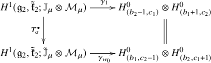
The diagram is not commutative! Proposition 4.20 says that it is commutative up to nonzero rational numbers and a particular ratio of archimedean L-values. The reader is referred to [27, Sect. 9.6].

4.2 The case of $\mathrm {{GL}}_N$

Now, we generalize Proposition 4.20, or as restated in Remark 4.21, to the case of $\mathrm {{GL}}_N,$ giving us the main result of this subsection in Proposition 4.32.

4.2.1 The induced representations and the standard intertwining operator

Take strongly-pure weights $\mu $ and $\mu '$ as in Section 3. Fix an archimedean place v (which we often drop simply to avoid tedious notation). Consider the induced representation

$$ \begin{align*}\sigma_v \ = \ \mathbb{J}_{\mu} \ = \ \mathrm{{Ind}}_{B_n(\mathbb{C})}^{\mathrm{{GL}}_n(\mathbb{C})} \left(z^{\alpha_1} \bar{z}^{\beta_1} \otimes \cdots \otimes z^{\alpha_n} \bar{z}^{\beta_n} \right), \quad \alpha_i, \beta_i \in \tfrac{(n-1)}{2} + \mathbb{Z}; \end{align*} $$

see (2.8) and (2.9) for the cuspidal parameters $\alpha _i$ and $\beta _i.$ Abbreviate this as

$$ \begin{align*}\sigma_v \ = \ \mathbb{J}_{\mu} \ = \ \psi_1 \times \cdots \times \psi_n; \quad \psi_i(z) = z^{\alpha_i} \bar{z}^{\beta_i}. \end{align*} $$

Similarly, we have

$$ \begin{align*}\sigma^{\prime}_v \ = \ \mathbb{J}_{\mu'} \ = \ \mathrm{{Ind}}_{B_{n'}(\mathbb{C})}^{\mathrm{{GL}}_{n'}(\mathbb{C})} \left(z^{\alpha^{\prime}_1} \bar{z}^{\beta^{\prime}_1} \otimes \cdots \otimes z^{\alpha^{\prime}_{n'}} \bar{z}^{\beta^{\prime}_{n'}} \right), \quad \alpha^{\prime}_j, \beta^{\prime}_j \in \tfrac{(n'-1)}{2} + \mathbb{Z}, \end{align*} $$

which we abbreviate as

$$ \begin{align*}\sigma^{\prime}_v \ = \ \mathbb{J}_{\mu'} \ = \ \psi^{\prime}_1 \times \cdots \times \psi^{\prime}_{n'}; \quad \psi^{\prime}_j(z) = z^{\alpha^{\prime}_j} \bar{z}^{\beta^{\prime}_j}. \end{align*} $$

We are interested in the standard intertwining operator

$$ \begin{align*}T_{\mathrm{st}} \ : \ {{}^{\mathrm{a}}\mathrm{Ind}}_{P_{(n,n')}(\mathbb{C})}^{\mathrm{{GL}}_N(\mathbb{C})}(\mathbb{J}_\mu \times \mathbb{J}_{\mu'}) \ \longrightarrow \ {{}^{\mathrm{a}}\mathrm{Ind}}_{P_{(n',n)}(\mathbb{C})} ^{\mathrm{{GL}}_N(\mathbb{C})} (\mathbb{J}_{\mu'}(-n) \times \mathbb{J}_\mu(n')). \end{align*} $$

which, in terms of normalized induced representations looks like

(4.25) $$ \begin{align} T_{\mathrm{st}} \ : \ \mathrm{{Ind}}_{P_{(n,n')}(\mathbb{C})}^{\mathrm{{GL}}_N(\mathbb{C})}(\mathbb{J}_\mu(-n'/2) \times \mathbb{J}_{\mu'}(n/2)) \ \longrightarrow \ \mathrm{{Ind}}_{P_{(n',n)}(\mathbb{C})} ^{\mathrm{{GL}}_N(\mathbb{C})} (\mathbb{J}_{\mu'}(n/2) \times \mathbb{J}_\mu(-n'/2)). \end{align} $$

Write

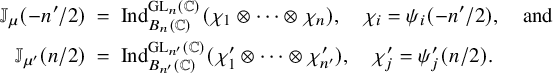$$ \begin{align*} \mathbb{J}_\mu(-n'/2) \ & = \ \mathrm{{Ind}}_{B_n(\mathbb{C})}^{\mathrm{{GL}}_n(\mathbb{C})}(\chi_1 \otimes \cdots \otimes \chi_n), \quad \chi_i = \psi_i(-n'/2), \quad \mathrm{and} \\ \mathbb{J}_{\mu'}(n/2) \ & = \ \mathrm{{Ind}}_{B_{n'}(\mathbb{C})}^{\mathrm{{GL}}_{n'}(\mathbb{C})}(\chi^{\prime}_1 \otimes \cdots \otimes \chi^{\prime}_{n'}), \quad \chi^{\prime}_j = \psi^{\prime}_j(n/2). \end{align*} $$

Apply transitivity of normalized induction to the representation in the domain of (4.25) to get

$$ \begin{align*} \mathrm{{Ind}}_{P_{(n,n')}(\mathbb{C})}^{\mathrm{{GL}}_N(\mathbb{C})} &\left( \mathrm{{Ind}}_{B_n(\mathbb{C})}^{\mathrm{{GL}}_n(\mathbb{C})}(\chi_1 \otimes \cdots \otimes \chi_n) \times \mathrm{{Ind}}_{B_{n'}(\mathbb{C})}^{\mathrm{{GL}}_{n'}(\mathbb{C})}(\chi^{\prime}_1 \otimes \cdots \otimes \chi^{\prime}_{n'}) \right) \ = \\ &\qquad \mathrm{{Ind}}_{B_N(\mathbb{C})}^{\mathrm{{GL}}_N(\mathbb{C})}(\chi_1 \otimes \cdots \otimes \chi_n \otimes \chi^{\prime}_1 \otimes \cdots \otimes \chi^{\prime}_{n'}) \ =: \ \chi_1 \times \cdots \times \chi_n \times \chi^{\prime}_1 \times \cdots \times \chi^{\prime}_{n'}, \end{align*} $$

and, similarly, the induced representation in the target is: $\chi ^{\prime }_1 \times \cdots \times \chi ^{\prime }_{n'} \times \chi _1 \times \cdots \times \chi _n.$ Hence, (4.25) takes the shape

(4.26) $$ \begin{align} T_{\mathrm{st}} \ : \ \chi_1 \times \cdots \times \chi_n \times \chi^{\prime}_1 \times \cdots \times \chi^{\prime}_{n'} \ \longrightarrow \ \chi^{\prime}_1 \times \cdots \times \chi^{\prime}_{n'} \times \chi_1 \times \cdots \times \chi_n. \end{align} $$

For a function $f \in \chi _1 \times \cdots \times \chi _n \times \chi ^{\prime }_1 \times \cdots \times \chi ^{\prime }_{n'}$ , we have the intertwining integral

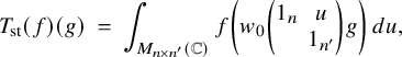(4.27) $$ \begin{align} T_{\mathrm{st}}(f)(g) \ = \ \int_{M_{n \times n'}(\mathbb{C})} f\left(w_0 \begin{pmatrix}1_n & u \\ & 1_{n'}\end{pmatrix} g \right) \, du, \end{align} $$

where $w_0$ is the element of the Weyl group of $\mathrm {{GL}}_N$ given by the following permutation:

$$ \begin{align*}w_0 \ = \ \begin{pmatrix} 1 & 2 & \dots & n-1 & n & n+1 & n+2 & \dots & N-1 & N \\ n'+1 & n'+2 & \dots & N-1 & N & 1 & 2 & \dots & n'-1 & n' \end{pmatrix}, \end{align*} $$

and the measure $du$ on $M_{n \times n'}(\mathbb {C})$ in the integral is taken as the product of the Lebesgue measures on each coordinate of u.

Proposition 4.28. Assume that the archimedean local factors $L(s, \mathbb {J}_\mu \times \mathbb {J}_{\mu '}^{\mathrm v})$ and $L(1-s, \mathbb {J}_\mu ^{\mathrm v} \times \mathbb {J}_{\mu '})$ are finite at $s = -N/2$ and $s=1-N/2.$ Then

1. 1. the representations $\chi _1 \times \cdots \times \chi _n \times \chi ^{\prime }_1 \times \cdots \times \chi ^{\prime }_{n'}$ and $\chi ^{\prime }_1 \times \cdots \times \chi ^{\prime }_{n'} \times \chi _1 \times \cdots \times \chi _n$ are irreducible; and furthermore,

2. 2. the standard intertwining integral $T_{\mathrm {st}}$ in (4.27) converges and gives an isomorphism between these two irreducible representations.

Proof. The proof follows from the Langlands–Shahidi machinery. For brevity, only for this proof, let $\sigma = \mathbb {J}_{\mu }$ and $\sigma ' = \mathbb {J}_{\mu '}.$ Let

$$ \begin{align*}I_P^G(s, \sigma \otimes \sigma') = \mathrm{Ind}_{P_{(n,n')}(\mathbb{C})}^{\mathrm{{GL}}_N(\mathbb{C})}((\sigma \otimes |\ |^{\frac{n'}{N}s}) \otimes ( \sigma' \otimes |\ |^{\frac{-n}{N}s})). \end{align*} $$

The s-variable is introduced using the fundamental weight corresponding to the simple root that is deleted for the maximal standard parabolic subgroup $P_{(n,n')}$ whose Levi quotient is the block diagonal subgroup $\mathrm {{GL}}_n \times \mathrm {{GL}}_{n'}.$ Similarly, we let

$$ \begin{align*}I_Q^G(-s, \sigma \otimes \sigma') = \mathrm{Ind}_{P_{(n',n)}(\mathbb{C})}^{\mathrm{{GL}}_N(\mathbb{C})}( ( \sigma' \otimes |\ |^{\frac{-n}{N}s}) \otimes (\sigma \otimes |\ |^{\frac{n'}{N}s})). \end{align*} $$

The standard intertwining operator $T_{\mathrm {st}}(s, w_0) : I_P^G(s, \sigma \otimes \sigma ') \to I_Q^G(-s, \sigma \otimes \sigma ')$ is given by the integral (4.27). Under the hypothesis of the proposition, it follows from Casselman–Shahidi [6, Prop. 5.3] that the induced representations $I_P^G(-N/2, \sigma \otimes \sigma ') = \chi _1 \times \cdots \times \chi _n \times \chi ^{\prime }_1 \times \cdots \times \chi ^{\prime }_{n'}$ and $I_Q^G(N/2, \sigma \otimes \sigma ') = \chi ^{\prime }_1 \times \cdots \times \chi ^{\prime }_{n'} \times \chi _1 \times \cdots \times \chi _n$ are irreducible. The operator $T_{\mathrm {st}} = T_{\mathrm {st}}(-N/2, w_0)$ being an isomorphism follows exactly as in the proof of [27, Prop. 7.54]; this part of the proof uses Shahidi’s results on local constants [46].

4.2.2 Factorizing the intertwining operator

For $1 \leq i \leq N-1$ , let ${\mathrm s}_i = (i, i+1)$ be the i-th simple reflection corresponding to the i-th simple root $\alpha _i = e_i-e_{i+1}.$ Its easy to see that a positive root $e_i - e_j$ (positivity is $i < j$ ) is mapped to a negative root by $w_0$ if and only if $1 \leq i \leq n$ and $n+1 \leq j \leq N,$ and hence $l(w_0) = nn'.$ Furthermore, its easy to see that

$$ \begin{align*}w_0 \ = \ ({\mathrm s}_{n'} \dots {\mathrm s}_2 {\mathrm s}_1) \cdots ({\mathrm s}_{N-2}\dots {\mathrm s}_n {\mathrm s}_{n-1}) ({\mathrm s}_{N-1}\dots {\mathrm s}_{n+1} {\mathrm s}_n), \end{align*} $$

where the right-hand side is grouped into n parenthetical expressions each of which is a product of $n'$ simple reflections, hence giving a minimal expression of $w_0$ in terms of $l(w_0)$ many simple reflections. This gives a factorization

(4.29) $$ \begin{align} T_{\mathrm{st}} = T_{\mathrm{st}}(w_0) = \left(T({\mathrm s}_{n'}) \circ \cdots \circ T({\mathrm s}_2)\circ T({\mathrm s}_1)\right) \circ \cdots \circ \left(T({\mathrm s}_{N-1}) \circ \cdots \circ T({\mathrm s}_{n+1})\circ T({\mathrm s}_n) \right), \end{align} $$

which is well known in the Langlands–Shahidi method; see, for example, [47, Thm. 4.2.2] as applied to our situation.

Example 4.30. To visualise such a factorisation, consider the simple but nontrivial example: take $n = 3$ and $n'=2$ . Then the right-hand side of (4.29) is the sequence of operators:

1. 1. $T({\mathrm s}_3) \ : \ \chi _1 \times \chi _2 \times \chi _3 \times \chi ^{\prime }_1 \times \chi ^{\prime }_2 \ \longrightarrow \ \chi _1 \times \chi _2 \times \chi ^{\prime }_1 \times \chi _3 \times \chi ^{\prime }_2$

2. 2. $T({\mathrm s}_4) \ : \ \chi _1 \times \chi _2 \times \chi ^{\prime }_1 \times \chi _3 \times \chi ^{\prime }_2 \ \longrightarrow \ \chi _1 \times \chi _2 \times \chi ^{\prime }_1 \times \chi ^{\prime }_2 \times \chi _3$

3. 3. $T({\mathrm s}_2) \ : \ \chi _1 \times \chi _2 \times \chi ^{\prime }_1 \times \chi ^{\prime }_2 \times \chi _3 \ \longrightarrow \ \chi _1 \times \chi ^{\prime }_1 \times \chi _2 \times \chi ^{\prime }_2 \times \chi _3$

4. 4. $T({\mathrm s}_3) \ : \ \chi _1 \times \chi ^{\prime }_1 \times \chi _2 \times \chi ^{\prime }_2 \times \chi _3 \ \longrightarrow \ \chi _1 \times \chi ^{\prime }_1 \times \chi ^{\prime }_2 \times \chi _2 \times \chi _3$

5. 5. $T({\mathrm s}_1) \ : \ \chi _1 \times \chi ^{\prime }_1 \times \chi ^{\prime }_2 \times \chi _2 \times \chi _3 \ \longrightarrow \ \chi ^{\prime }_1 \times \chi _1 \times \chi ^{\prime }_2 \times \chi _2 \times \chi _3$

6. 6. $T({\mathrm s}_2) \ : \ \chi ^{\prime }_1 \times \chi _1 \times \chi ^{\prime }_2 \times \chi _2 \times \chi _3 \ \longrightarrow \ \chi ^{\prime }_1 \times \chi ^{\prime }_2 \times \chi _1\times \chi _2 \times \chi _3.$

The point is that at every intermediate stage, there are only two characters $\chi _i$ and $\chi ^{\prime }_j$ that are getting switched. The corresponding integral is happening over the coordinate $u_{ij}$ in the variable $u \in M_{n \times n'}(\mathbb {C})$ that appears in (4.27). The measure $du$ , as mentioned above, is the product of the Lebesgue measures $du_{ij}.$ Such an intermediate integral is the induction to $\mathrm {{GL}}_N$ of a $\mathrm {{GL}}_2$ -intertwining integral, and we have seen that it corresponds to scaling by a factor $L_\infty (0, \chi _i \chi _j^{\prime -1})/L_\infty (1, \chi _i \chi _j^{\prime -1})$ (up to a nonzero rational). This implies that $T_{\mathrm {st}}$ will have a scaling factor of the product of all intermediate scaling factors, towards which note the easy lemma:

Lemma 4.31.

$$ \begin{align*}\prod_{i=1}^n \prod_{j=1}^{n'} \frac{L_\infty(0, \chi_i \chi_j^{\prime -1})}{L_\infty(1, \chi_i \chi_j^{\prime -1})} \ = \ \prod_{i=1}^n \prod_{j=1}^{n'} \frac{L_\infty(-\tfrac{N}{2}, \psi_i \psi_j^{\prime -1})}{L_\infty(1-\tfrac{N}{2}, \psi_i \psi_j^{\prime -1})} \ = \ \frac{L_\infty(-\tfrac{N}{2}, \sigma_\infty \times \sigma_\infty^{\prime \mathrm v})}{L_\infty(1-\tfrac{N}{2}, \sigma_\infty \times \sigma_\infty^{\prime \mathrm v})}. \end{align*} $$

4.2.3 The intertwining operator in cohomology

Let ${\mathscr {J}} = {\mathscr {J}}^0$ stand for the underlying $(\mathfrak {g}_N,{\mathfrak {k}}_N)$ -module of $\mathrm {{Ind}}_{B_N(\mathbb {C})}^{\mathrm {{GL}}_N(\mathbb {C})}( \chi _1 \otimes \cdots \otimes \chi _n \otimes \chi ^{\prime }_1 \otimes \cdots \otimes \chi ^{\prime }_{n'})$ , and similarly, $\tilde {\mathscr {J}} = {\mathscr {J}}^{nn'}$ that of $\mathrm {{Ind}}_{B_N(\mathbb {C})}^{\mathrm {{GL}}_N(\mathbb {C})}( \chi ^{\prime }_1 \otimes \cdots \otimes \chi ^{\prime }_{n'} \otimes \chi _1 \otimes \cdots \otimes \chi _n).$ Rewrite the factorization in (4.29) as

$$ \begin{align*}T_{\mathrm{st}} = T^{nn'} \circ \cdots \circ T^2 \circ T^1, \quad T^k : {\mathscr{J}}^{k-1} \to {\mathscr{J}}^k \ \mbox{for } 1 \leq k \leq nn'. \end{align*} $$

with each ${\mathscr {J}}^k$ being an irreducible principal series representation, and each $T^k$ is the induction of a $\mathrm {{GL}}_2$ -intertwining operator as explained. Note that

$$ \begin{align*}\mathrm{{Ind}}_{B_N(\mathbb{C})}^{\mathrm{{GL}}_N(\mathbb{C})}(\chi_1 \otimes \cdots \otimes \chi_n \otimes \chi^{\prime}_1 \otimes \cdots \otimes \chi^{\prime}_{n'}) = {{}^{\mathrm{a}}\mathrm{Ind}}_{B_N(\mathbb{C})}^{\mathrm{{GL}}_N(\mathbb{C})}(\xi_1 \otimes \cdots \otimes \xi_n \otimes \xi^{\prime}_1 \otimes \cdots \otimes \xi^{\prime}_{n'}), \end{align*} $$

where $\xi _i = \chi _i\left (\tfrac {N-2i+1}{2}\right ) = \psi _i\left (\tfrac {n-2i+1}{2}\right )$ and $\xi ^{\prime }_j = \chi ^{\prime }_j\left (\tfrac {N-2j-2n+1}{2}\right ) = \psi ^{\prime }_j\left (\tfrac {n'-2j+1}{2}\right )$ are all algebraic characters of $\mathbb {C}^{\times }$ . Similarly, each ${\mathscr {J}}^k$ is the algebraic parabolic induction of an algebraic character of the diagonal torus. Delorme’s lemma identifies the one-dimensional cohomology group $H^{b_N^{\mathbb {C}}}(\mathfrak {g}_N, {\mathfrak {k}}_N; {\mathscr {J}}^k \otimes \mathcal {M}_\lambda )$ as a tensor product of the $\mathrm {{GL}}_1$ cohomology groups for the $\xi _i$ ’s and $\xi _j^{\prime }$ ’s; as in (4.23), but simplifying notations, we have

$$ \begin{align*}\gamma_k : H^{b_N^{\mathbb{C}}}(\mathfrak{g}_N, {\mathfrak{k}}_N; {\mathscr{J}}^k \otimes \mathcal{M}_\lambda) \ \stackrel{\approx}{\longrightarrow} \ (\mbox{product of } \mathrm{{GL}}_1 \mbox{ cohomology groups}). \end{align*} $$

This product of $\mathrm {{GL}}_1$ -cohomology groups may be identified with each other for $1 \leq k \leq nn'.$ Fixing a rational basis $\omega _{(b,c)}$ for each of the $\mathrm {{GL}}_1$ -classes and so for their tensor product, we define a basis element $[{\mathscr {J}}^k]_0$ for $H^{b_N^{\mathbb {C}}}(\mathfrak {g}_N, {\mathfrak {k}}_N; {\mathscr {J}}^k \otimes \mathcal {M}_\lambda )$ via $\gamma _k^{-1}.$

We start with $T^1 : {\mathscr {J}}^0 \to {\mathscr {J}}^1$ and note that this is the induction from $(n-1, 2, n'-1)$ -parabolic subgroup of $\mathrm {{GL}}_N$ of the $\mathrm {{GL}}_2$ -intertwining operator that switches $\chi _n$ and $\chi ^{\prime }_1$ . Proposition 4.20 applied to $T^1$ gives

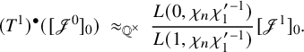$$ \begin{align*}(T^1)^{\bullet} ([{\mathscr{J}}^0]_0) \ \approx_{\mathbb{Q}^{\times}} \ \frac{L(0, \chi_n \chi^{\prime}_1{}^{-1})}{L(1, \chi_n \chi^{\prime}_1{}^{-1})} [{\mathscr{J}}^1]_0. \end{align*} $$

At the next step, from the factorisation in (4.29), we will get

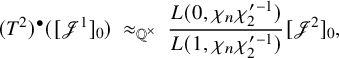$$ \begin{align*}(T^2)^{\bullet} ([{\mathscr{J}}^1]_0) \ \approx_{\mathbb{Q}^{\times}} \ \frac{L(0, \chi_n \chi^{\prime}_2{}^{-1})}{L(1, \chi_n \chi^{\prime}_2{}^{-1})} [{\mathscr{J}}^2]_0, \end{align*} $$

and so on. Using Lemma 4.31, Proposition 4.20 generalizes to the following:

Proposition 4.32.

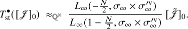$$ \begin{align*}T_{\mathrm{st}}^{\bullet}([{\mathscr{J}}]_0) \ \approx_{\mathbb{Q}^{\times}} \ \frac{L_\infty(-\tfrac{N}{2}, \sigma_\infty \times \sigma_\infty^{\prime \mathrm v})}{L_\infty(1-\tfrac{N}{2}, \sigma_\infty \times \sigma_\infty^{\prime \mathrm v})} \, [\tilde {\mathscr{J}}]_0. \end{align*} $$

The reader is referred to Harder [25] where a hope is expressed in general, and verified in the context therein, that the rational number implicit in $\approx _{\mathbb {Q}^{\times }}$ has a simple shape. See (4.17) and (4.18) above in the simplest possible case of $n = n' = 1.$

5 The main theorem on special values of L-functions for $\mathrm {{GL}}_n \times \mathrm {{GL}}_{n'}$

Before the main theorem on L-values (Theorem 5.16) can be stated and proved, two technical results on the boundary cohomology are necessary; the first is what is known as a ‘Manin–Drinfeld’ principle and the second is on rank-one Eisenstein cohomology.

5.1 A Manin–Drinfeld Principle

The main purpose of this subsection is to state and prove Theorem 5.5.

5.1.1 Kostant representatives

To begin, two important lemmas about Kostant representatives from [27, Sect. 5.3.2] are recorded below. Recall that $P = \mathrm {Res}_{F/\mathbb {Q}}(P_0)$ and $P_0 = P_{(n,n')}$ is the maximal parabolic subgroup of type $(n,n')$ of $G_0 = \mathrm {{GL}}_N/F.$ Let $Q_0 = P_{(n',n)}$ be the associate parabolic, and $Q = \mathrm {Res}_{F/\mathbb {Q}}(Q_0)$ . Let $\mathbf {\Pi }_{M_{P_0}} = \mathbf {\Pi }_{G_0} - \{\alpha _{P_0}\}$ . Let $w_{P_0}$ be the unique element of $W_0 = W_{G_0}$ such that $w_{P_0}(\mathbf {\Pi }_{M_{P_0}}) \subset \mathbf {\Pi }_{G_0}$ and $w_{P_0}(\alpha _{P_0}) < 0,$ it is the longest Kostant representative for $W^{P_0}.$

Lemma 5.1. With notations as above, one has

1. 1. The map $w \mapsto w^\prime := w_{P}\,w$ gives a bijection $W^P \to W^Q$ . If $w= (w^\tau )_{\tau : F \to E}$ , then by definition, $w_{P}w = (w_{P_0}w^\tau )_{\tau :F \to E}.$

2. 2. This bijection has the property that $l(w^\tau ) + l(w^{\prime \tau }) = \dim {(U_{P_0^\tau })}$ .

3. 3. w is balanced if and only if $w'$ is balanced.

Similarly, there is the following self-bijection of $W^P$ :

Lemma 5.2. Let $w_G$ be the element of longest length in the Weyl group $W_G$ of G, and similarly, let $w_{M_P}$ be the element of longest length in the Weyl group $W_{M_P}$ . Then

1. 1. The map $w \mapsto w^{\mathrm v}:= w_{M_P}\cdot w \cdot w_G$ gives a bijection $W^P \to W^P$ .

2. 2. This bijection has the property that $l(w^\tau ) + l(w^{{\mathrm {v}}\tau }) = \dim {(U_{P_0^\tau })}.$

3. 3. w is balanced if and only if $w^{\mathrm {v}}$ is balanced.

5.1.2 Induced representations in boundary cohomology

The conditions imposed by the combinatorial lemma (Lemma 3.16) have a consequence on the occurrences of induced representations as Hecke summands in the boundary cohomology. Recall that E is a large enough Galois extension of $\mathbb {Q}$ that takes a copy of F. Consider strongly-pure weights $\mu \in X^+_{00}(T_n \times E)$ and $\mu ' \in X^+_{00}(T_{n'} \times E).$ Let $\sigma _f \in \mathrm {{Coh}}_{!!}(G_n, \mu )$ and $\sigma ^{\prime }_f \in \mathrm {{Coh}}_{!!}(G_{n'}, \mu ')$ be strongly-inner Hecke-summands. The effect of the related balanced representatives: $w', w^{\mathrm {v}}$ and $w^{\mathrm {v}}{}'$ on certain weights are recorded in the following:

Proposition 5.3. Assume that the weights $\mu $ and $\mu '$ satisfy the conditions of the combinatorial lemma (Lemma 3.16). Hence, there is a balanced element $w \in W^P$ such that $\lambda := w^{-1} \cdot (\mu + \mu ')$ is dominant. Then (after recalling the notations in Section 2.4.1),

1. 1.

2. 2. and

3. 3. $w^{\mathrm {v}}{}' \cdot \lambda ^{\mathrm {v}} = \mu ^{\prime \mathrm {v}} + \mu ^{\mathrm {v}}.$

For a proof of the above proposition, the reader is referred to [27, Sect. 5.3.4]. The appearance of various induced modules in boundary cohomology in bottom and top degrees are recorded in the following:

Proposition 5.4. Let the notations be as above.

1. 1. The module ${{}^{\mathrm {a}}\mathrm {Ind}}_{P(\mathbb {A}_f)}^{G(\mathbb {A}_f)}(\sigma _f \times \sigma ^{\prime }_f)$ appears in $H^{{\mathrm {q}}_b}(\partial _P\mathcal {S}^G, \widetilde {\mathcal {M}}_{\lambda , E}),$

   where ${\mathrm {q}}_b = b_N^F = b_n^F + b_{n'}^F + \frac 12 \dim (U_P).$

2. 2. The module ${{}^{\mathrm {a}}\mathrm {Ind}}_{Q(\mathbb {A}_f)}^{G(\mathbb {A}_f)}(\sigma ^{\prime }_f(n) \times \sigma _f(-n'))$ appears in $H^{{\mathrm {q}}_b}(\partial _Q\mathcal {S}^G, \widetilde {\mathcal {M}}_{\lambda ,E}).$

The contragredient of the algebraically-induced modules is

$$ \begin{align*}{{}^{\mathrm{a}}\mathrm{Ind}}_{P(\mathbb{A}_f)}^{G(\mathbb{A}_f)}(\sigma_f \times \sigma^{\prime}_f)^{\mathrm{v}} \ = \ {{}^{\mathrm{a}}\mathrm{ Ind}}_{P(\mathbb{A}_f)}^{G(\mathbb{A}_f)}(\sigma_f^{\mathrm{v}}(n') \times \sigma^{\prime \mathrm{v}}_f(-n)). \end{align*} $$

Furthermore, for the contragredients and cohomology in top-degree, we have

1. (3) ${{}^{\mathrm {a}}\mathrm {Ind}}_{P(\mathbb {A}_f)}^{G(\mathbb {A}_f)}(\sigma _f^{\mathrm {v}}(n') \times \sigma ^{\prime \mathrm {v}}_f(-n))$ appears in $H^{{\mathrm {q}}_t}(\partial _P\mathcal {S}^G, \widetilde {\mathcal {M}}_{\lambda ^{\mathrm {v}}, E}),$

   where ${\mathrm {q}}_t = t_N^F - 1 = t_n^F + t_{n'}^F + \frac 12 \dim (U_P).$

2. (4) ${{}^{\mathrm {a}}\mathrm {Ind}}_{Q(\mathbb {A}_f)}^{G(\mathbb {A}_f)}(\sigma ^{\prime \mathrm {v}}_f \times \sigma _f^{\mathrm {v}} )$ appears in $H^{{\mathrm {q}}_t}(\partial _Q\mathcal {S}^G, \widetilde {\mathcal {M}}_{\lambda ^{\mathrm {v}}, E}).$

Proof. For (1), use the summand in Proposition 2.25 indexed by the balanced Kostant representative $w \in W^P$ provided by Lemma 3.16. For (2), use $w' \in W^Q$ from Lemma 5.1, and then use (1) of Proposition 5.3. For (3), use $w^{\mathrm {v}} \in W^P$ from Lemma 5.2, and then use (2) of Proposition 5.3. For (4), use $w^{\mathrm {v}}{}' \in W^Q$ from Lemma 5.1 and 5.2, and (3) of Proposition 5.3. The assertions of the cohomology degrees is clear from Proposition 2.15 and 2.16.

5.1.3 The Manin–Drinfeld principle

Continue with the notations $\mu \in X^+_{00}(T_n \times E)$ , $\mu ' \in X^+_{00}(T_{n'} \times E)$ , $\sigma _f \in \mathrm {{Coh}}_{!!}(G_n, \mu )$ , and $\sigma ^{\prime }_f \in \mathrm {{Coh}}_{!!}(G_{n'}, \mu ').$ Assume that $\mu $ and $\mu '$ satisfy the conditions of the combinatorial lemma (Lemma 3.16), and let $\lambda = w^{-1}\cdot (\mu +\mu ').$ Let $K_f$ be an open-compact subgroup of $G(\mathbb {A}_f)$ such that ${{}^{\mathrm {a}}\mathrm {Ind}}_{P(\mathbb {A}_f)}^{G(\mathbb {A}_f)}(\sigma _f \times \sigma ^{\prime }_f)$ has nonzero $K_f$ -fixed vectors; suppose ${\mathrm k}$ is the dimension of these $K_f$ -fixed vectors. Let

$$ \begin{align*}I_b^{\mathrm{S}}(\sigma_f, \sigma^{\prime}_f)_{P, w} \ := \ {{}^{\mathrm{a}}\mathrm{Ind}}_{P(\mathbb{A}_f)}^{G(\mathbb{A}_f)} \left(H^{b_n^F+b_{n'}^F}(\mathcal{S}^{M_P}, \widetilde{\mathcal{M}}_{w \cdot \lambda})(\sigma_f \times \sigma^{\prime}_f) \right)^{K_f}, \end{align*} $$

and similarly, define

$$ \begin{align*}I_b^{\mathrm{S}}(\sigma^{\prime}_f(n) , \sigma_f(-n'))_{Q, w'} \ := \ {{}^{\mathrm{a}}\mathrm{Ind}}_{Q(\mathbb{A}_f)}^{G(\mathbb{A}_f)} \left(H^{b_n^F+b_{n'}^F}(\mathcal{S}^{M_Q}, \widetilde{\mathcal{M}}_{w' \cdot \lambda})(\sigma^{\prime}_f(n) \times \sigma_f(-n')) \right)^{K_f}. \end{align*} $$

Now, go to ‘top-degree’ for the contragredient modules and define

$$ \begin{align*}I_t^{\mathrm{S}}(\sigma_f^{\mathrm{v}}(n') , \sigma^{\prime \mathrm{v}}_f(-n))_{P, w^{\mathrm{v}}} \ := \ {{}^{\mathrm{a}}\mathrm{Ind}}_{P(\mathbb{A}_f)}^{G(\mathbb{A}_f)} \left(H^{t_n^F+t_{n'}^F}(\mathcal{S}^{M_P}, \widetilde{\mathcal{M}}_{w^{\mathrm{v}} \cdot \lambda})(\sigma_f^{\mathrm{v}}(n') \times \sigma^{\prime \mathrm{v}}_f(-n)) \right)^{K_f}, \end{align*} $$

and similarly, define

$$ \begin{align*}I_t^{\mathrm{S}}(\sigma^{\prime \mathrm{v}}_f , \sigma_f^{\mathrm{v}})_{Q, w^{\mathrm{v}}{}'} \ := \ {{}^{\mathrm{a}}\mathrm{Ind}}_{Q(\mathbb{A}_f)}^{G(\mathbb{A}_f)} \left(H^{t_n^F+t_{n'}^F}(\mathcal{S}^{M_Q}, \widetilde{\mathcal{M}}_{w^{\mathrm{v}}{}' \cdot \lambda})(\sigma^{\prime \mathrm{v}}_f \times \sigma_f^{\mathrm{v}} ) \right)^{K_f}. \end{align*} $$

Theorem 5.5. Let the notations be as above.

1. 1. The sum

   $$ \begin{align*}I_b^{\mathrm{S}}(\sigma_f, \sigma^{\prime}_f)_{P, w} \ \oplus \ I_b^{\mathrm{S}}(\sigma^{\prime}_f(n) , \sigma_f(-n'))_{Q, w'} \end{align*} $$
   is a $2{\mathrm k}$ -dimensional E-vector space that is isotypic in $H^{q_b}(\partial \mathcal {S}^G_{K_f}, \widetilde {\mathcal {M}}_{\lambda ,E}).$ Note that if $Q = P$ , then $w' \neq w.$ Furthermore, there is a $\mathcal {H}^{G,\mathrm {S}}$ -equivariant projection
   $$ \begin{align*}\mathfrak{R}^b_{\sigma_f, \sigma^{\prime}_f} \ : \ H^{q_b}(\partial\mathcal{S}^G_{K_f}, \widetilde{\mathcal{M}}_{\lambda,E}) \ \longrightarrow \ I_b^{\mathrm{S}}(\sigma_f, \sigma^{\prime}_f)_{P, w} \oplus I_b^{\mathrm{S}}(\sigma^{\prime}_f(n) , \sigma_f(-n'))_{Q, w'}. \end{align*} $$

2. 2. Similarly, in ‘top-degree’, the sum

   $$ \begin{align*}I_t^{\mathrm{S}}(\sigma_f^{\mathrm{v}}(n') , \sigma^{\prime \mathrm{v}}_f(-n))_{P, w^{\mathrm{v}}} \ \oplus \ I_t^{\mathrm{S}}(\sigma^{\prime \mathrm{v}}_f , \sigma_f^{\mathrm{v}})_{Q, w^{\mathrm{v}}{}'} \end{align*} $$
   is a $2{\mathrm k}$ -dimensional E-vector space that is isotypic in $H^{q_t}(\partial \mathcal {S}^G_{K_f}, \widetilde {\mathcal {M}}_{\lambda ^{\mathrm {v}},E}).$ Note that if $Q = P$ , then $w^{\mathrm {v}}{}' \neq w^{\mathrm {v}}.$ Furthermore, there is a $\mathcal {H}^{G,\mathrm {S}}$ -equivariant projection
   $$ \begin{align*}\mathfrak{R}^t_{\sigma_f, \sigma^{\prime}_f} \ : \ H^{q_t}(\partial\mathcal{S}^G_{K_f}, \widetilde{\mathcal{M}}_{\lambda^{\mathrm{v}}, E}) \ \longrightarrow \ I_t^{\mathrm{S}}(\sigma_f^{\mathrm{v}}(n') , \sigma^{\prime \mathrm{v}}_f(-n))_{P, w^{\mathrm{v}}} \oplus I_t^{\mathrm{S}}(\sigma^{\prime \mathrm{v}}_f , \sigma_f^{\mathrm{v}})_{Q, w^{\mathrm{v}}{}'}. \end{align*} $$

The above theorem is the exact analogue of [27, Thm. 5.12], and the proof is identical. To help the reader, the two key-ideas are adumbrated as follows:

• ○ There is a spectral sequence – built from the cohomology of various boundary strata $\partial _R\mathcal {S}^G$ , as R runs over $G(\mathbb {Q})$ -conjugacy classes of parabolic subgroups of G – that converges to the boundary cohomology $H^{\bullet }(\partial \mathcal {S}^G, -)$ . This spectral sequence was alluded to in Section 2.6 and is discussed in greater detail in [27, Sect. 4.1]. The basic idea here is that up to semi-simplification the cohomology of the boundary is built from parabolically induced representations.

• ○ Recall the strong multiplicity one theorem of Jacquet and Shalika for isobaric automorphic representations [32, Thm. 4.4]. The two induced modules in $I_b^{\mathrm {S}}(\sigma _f, \sigma ^{\prime }_f)_{P, w}$ and $I_b^{\mathrm {S}}(\sigma ^{\prime }_f(n) , \sigma _f(-n'))_{Q, w'}$ are themselves, of course, $\mathcal {H}^{G,\mathrm {S}}$ -equivalent, and more importantly, after applying Jacquet–Shalika, they are not almost-everywhere equivalent to any other induced module anywhere else in boundary cohomology; see [27, Sect. 5.3.3] for more details.

5.2 Eisenstein cohomology

All the statements in [27, Chap. 6] go through mutatis mutandis in the current situation. Therefore, the discussion below is very brief and just enough details are provided for this article to be reasonably self-contained, and to be able to state the main theorem on rank-one Eisenstein cohomology in Theorem 5.6 below.

5.2.1 Poincaré duality and consequences

The Poincaré duality pairings on $\mathcal {S}^G_{K_f}$ and $\partial \mathcal {S}^G_{K_f}$ are compatible with the maps in the long exact sequence in Section 2.1:

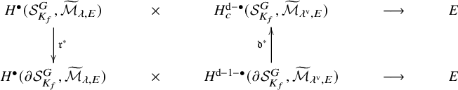
Here, $\mathrm {dim}(\mathcal {S}^G_{K_f}) = b_N^F + t_N^F =: {\mathrm {d}}$ ; and so $\mathrm { dim}(\partial \mathcal {S}^G_{K_f}) = {\mathrm {d}} -1 = {\mathrm {q}}_b + {\mathrm {q}}_t.$ A consequence of the above diagram is that Eisenstein cohomology, defined as

$$ \begin{align*}H^q_{\mathrm{Eis}}(\partial\mathcal{S}^G_{K_f}, \widetilde{\mathcal{M}}_{\lambda, E}) \ := \ \mathrm{Image} \left(H^q(\mathcal{S}^G_{K_f}, \widetilde{\mathcal{M}}_{\lambda, E}) \stackrel{{\mathfrak{r}}^{\bullet}}{\longrightarrow} H^q(\partial\mathcal{S}^G_{K_f}, \widetilde{\mathcal{M}}_{\lambda, E}) \right), \end{align*} $$

is a maximal isotropic subspace of boundary cohomology; that is,

$$ \begin{align*}H^q_{\mathrm{{Eis}}}(\partial\mathcal{S}^G_{K_f}, \widetilde{\mathcal{M}}_{\lambda, E}) \ = \ H^{{\mathrm{d}}-1-q}_{\mathrm{{Eis}}}(\partial\mathcal{S}^G_{K_f}, \widetilde{\mathcal{M}}_{\lambda^{\mathrm{v}}, E})^\perp. \end{align*} $$

5.2.2 Main result on rank-one Eisenstein cohomology

With notations as in Section 5.1.3, consider the following maps starting from global cohomology $H^{q_b}( \mathcal {S}^G_{K_f},\widetilde {\mathcal {M}}_{\lambda ,E})$ and ending with an isotypic component in boundary cohomology:

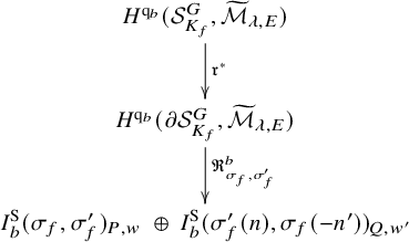
Recall from Theorem 5.5 that $I^{\mathrm {S}}_b({{\sigma }_f},{\sigma }^{\prime }_f)_{P, w} \oplus I^{\mathrm {S}}_b(\sigma _f^{\prime }(n), \sigma _f(-n'))_{Q, w^\prime }$ is a E-vector space of dimension $2{\mathrm k}$ . In the self-associate case, replace Q by P. The proof of the main result on Eisenstein cohomology stated below also needs the analogue of the above maps for cohomology in degree $q_t$ for the coefficient system $\widetilde {\mathcal {M}}_{\lambda ^{\mathrm {v}},E}.$

Theorem 5.6. For brevity, let

$$ \begin{align*}\mathfrak{I}^b(\sigma_f, \sigma_f^{\prime}) \ := \ \mathfrak{R}_{\sigma_f, \sigma^{\prime}_f}^b(H^{{\mathrm{q}}_b}_{\mathrm{{Eis}}}(\partial\mathcal{S}^G_{K_f}, \widetilde{\mathcal{M}}_{\lambda,E})), \quad \mathfrak{I}^t(\sigma_f, \sigma_f^{\prime})^{\mathrm{v}} \ := \ \mathfrak{R}_{\sigma_f, \sigma^{\prime}_f}^t(H^{{\mathrm{q}}_t}_{\mathrm{{Eis}}}(\partial\mathcal{S}^G_{K_f},\widetilde{\mathcal{M}}_{\lambda^{\mathrm{v}},E})). \end{align*} $$

1. 1. In the non-self-associate cases ( $n \neq n'$ ), we have

   1. (a) $\mathfrak {I}^b(\sigma _f, \sigma _f^{\prime })$ is an E-subspace of dimension ${\mathrm k}$ .

   2. (b) $\mathfrak {I}^t(\sigma _f, \sigma _f^{\prime })^{\mathrm {v}}$ is an E-subspace of dimension ${\mathrm k}$ .

2. 2. In the self-associate case ( $n=n'$ ), the same assertions hold by putting $Q = P.$

It helps to have a mental picture of when ${\mathrm k} = 1$ (i.e., then $\mathfrak {I}^b(\sigma _f, \sigma _f^{\prime })$ is a line in the ambient two-dimensional space $I^{\mathrm {S}}_b({{\sigma }_f},{\sigma }^{\prime }_f)_{P, w} \oplus I^{\mathrm {S}}_b(\sigma _f^{\prime }(n), \sigma _f(-n'))_{Q, w^\prime }$ ); as will be seen later, the ‘slope’ of this line contains arithmetic information about L-values.

A very brief sketch of proof.

The proof works exactly as explained in [27, Sect. 6.2.2], and involves two basic steps:

1. (i) The first step is to show that both $\mathfrak {I}^b(\sigma _f, \sigma _f^{\prime })$ and $\mathfrak {I}^t(\sigma _f, \sigma _f^{\prime })^{\mathrm {v}}$ have dimension at least ${\mathrm k}$ ; this is achieved by going to a transcendental level and appealing to Langlands’s constant term theorem and producing enough cohomology classes in the image. The essential features are reviewed in Section 5.2.3 below, and for more details, the reader is referred to [27, Sect. 6.3.7].

2. (ii) The second step, after invoking properties of the Poincaré duality pairing reviewed above, is to show that both $\mathfrak {I}^b(\sigma _f, \sigma _f^{\prime })$ and $\mathfrak {I}^t(\sigma _f, \sigma _f^{\prime })^{\mathrm {v}}$ have dimension exactly ${\mathrm k}.$ This step works exactly as in [27, Sect. 6.2.2.2].

5.2.3 L-values and rank-one Eisenstein cohomology

The key ingredient in the main theorem on the rationality of these L-values is the role played by the L-values in the above result on rank-one Eisenstein cohomology.

Induced representations

Let $\sigma $ (resp., $\sigma '$ ) be a cuspidal automorphic representation of $G_n(\mathbb {A})$ (resp., $G_{n'}(\mathbb {A})$ ). The relation with the previous ‘arithmetic’ notation is that given $\sigma _f \in \mathrm {{Coh}}_{!!}(G_n,\mu )$ and given $\iota : E \to \mathbb {C}$ , think of ${}^\iota \sigma _f$ to be the finite part of a cuspidal automorphic representation ${}^\iota \sigma $ , etc. The $\iota $ is fixed and it is suppressed until otherwise mentioned. Consider the induced representation $I_P^G(s, \sigma \otimes \sigma ')$ consisting of all smooth functions $f : G(\mathbb {A}) \to V_{ \sigma } \otimes V_{ \sigma '}$ such that

(5.7) $$ \begin{align} f(mug) \ = \ \vert\delta_P\vert(m)^{\frac{1}{2}} \vert\delta_P\vert(m)^{\frac{s}{N}} \, ( \sigma \otimes \sigma')(m) \, f(g), \end{align} $$

for all $m \in M_P(\mathbb {A})$ , $u \in U_P(\mathbb {A})$ and $g \in G(\mathbb {A})$ ; where $V_\sigma $ (resp., $V_{\sigma '}$ ) is the subspace inside the space of cusp forms on $G_n(\mathbb {A})$ (resp., $G_{n'}(\mathbb {A})$ ) realizing the representation $ \sigma $ (resp., $ \sigma '$ ). In other words, $I_P^G(s, \sigma \otimes \sigma ') = {\mathrm {Ind}}_{P(\mathbb {A})}^{G(\mathbb {A})}((\sigma \otimes |\ |^{\frac {n'}{N}s}) \otimes ( \sigma ' \otimes |\ |^{\frac {-n}{N}s})),$ where ${\mathrm {Ind}}_P^G$ denotes the normalized parabolic induction. In terms of algebraic or un-normalized induction, we have

(5.8) $$ \begin{align} I_P^G(s, \sigma \otimes \sigma') = {}^{\mathrm a}{\mathrm{Ind}}_{P(\mathbb{A})}^{G(\mathbb{A})} (( \sigma \otimes |\ |^{\frac{n'}{N}s + \frac{n'}{2}}) \otimes ( \sigma' \otimes |\ |^{\frac{-n}{N}s - \frac{n}{2}})). \end{align} $$

Specifically, note the point of evaluation $s_0 = -N/2$ :

$$ \begin{align*}{}^{\mathrm a}{\mathrm{Ind}}_{P(\mathbb{A})}^{G(\mathbb{A})} \left( \sigma \otimes \sigma' \right) \ = \ I_P^G(s, \sigma \otimes \sigma')|_{s = -N/2}, \ \ {}^{\mathrm a}{\mathrm{Ind}}_{Q(\mathbb{A})}^{G(\mathbb{A})} \left( \sigma'(n) \otimes \sigma(-n') \right) \ = \ I_Q^G(s, \sigma' \otimes \sigma)|_{s = N/2}. \end{align*} $$

The finite parts of the induced representations appear in boundary cohomology.

Standard intertwining operators

There is an element $w_{P} \in W_G$ , the Weyl group of G, which is uniquely determined by the property and If we write $w_{P} = (w_{P_0}^\tau )_{\tau :F \to E}$ , then for each $\tau $ , as a permutation matrix in $\mathrm {{GL}}_N$ , we have $w_{P_0}^\tau = \left [\begin {smallmatrix}& 1_n \\ 1_{n'} & \end {smallmatrix}\right ].$ The parabolic subgroup Q, which is associate to P, corresponds to Since $w_{P_0}^\tau \!{}^{-1} \, \mathrm {diag}(h,h') \, w_{P_0}^\tau = \mathrm {diag}(h',h)$ for all $ \mathrm {diag}(h,h') \in M_{P_0^\tau }$ , we get $w_{P}(\sigma \otimes \sigma ') = \sigma ' \otimes \sigma $ as a representation of $M_{Q}(\mathbb {A})$ . The global standard intertwining operator

$$ \begin{align*}T_{\mathrm{st}}^{PQ}(s, \sigma \otimes \sigma') : I_P^G(s, \sigma \otimes \sigma') \ \longrightarrow \ I_Q^G(-s, \sigma' \otimes \sigma) \end{align*} $$

is given by the integral

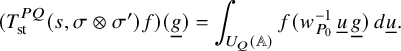(5.9) $$ \begin{align} (T_{\mathrm{st}}^{PQ}(s, \sigma \otimes \sigma')f)(\underline g) = \int_{U_{Q}(\mathbb{A})}f(w_{P_0}^{-1} \, \underline u \, \underline g)\, d\underline u. \end{align} $$

See 5.2.3 for the choice of measure $d \underline u.$ Abbreviate $T_{\mathrm {st}}^{PQ}(s, \sigma \otimes \sigma ')$ as $T_{\mathrm {st}}(s, \sigma \otimes \sigma ').$ The global standard intertwining operator factorizes as a product of local standard intertwining operators: $T_{\mathrm {st}}(s, \sigma \otimes \sigma ') = \otimes _v T_{\mathrm {st}}(s, \sigma _v \otimes \sigma ^{\prime }_v)$ , where the local operator is given by a similar local integral. (At an archimedean place, the effect of this operator in relative Lie algebra cohomology has already been described in Section 4.)

Eisenstein series

Let $f \in I_P^G(s, \sigma \times \sigma ^\prime )$ , for $\underline g \in G(\mathbb {A})$ the value $f(\underline g)$ is a cusp form on $M_P(\mathbb {A}).$ By the defining equivariance property of f, the complex number $f(\underline g)(\underline m)$ determines and is determined by $f(\underline m \underline g)(\underline 1)$ for any $\underline m \in M_P(\mathbb {A}).$ Henceforth, $f \in I_P^G(s, \sigma \times \sigma ')$ will be identified with the complex valued function $\underline g \mapsto f(\underline g)(\underline 1);$ that is, one has embedded

$$ \begin{align*}I_P^G(s, \sigma \times \sigma^\prime) \ \hookrightarrow \ \mathcal{C}^\infty\left(U_P(\mathbb{A})M_P(\mathbb{Q})\backslash G(\mathbb{A}), \omega_\infty^{-1}\right) \ \subset \ \mathcal{C}^\infty\left(P(\mathbb{Q})\backslash G(\mathbb{A}), \omega_\infty^{-1}\right), \end{align*} $$

where $\omega ^{-1}_\infty $ is a simplified notation for the central character of $\sigma \otimes \sigma '$ restricted to $S(\mathbb {R})^\circ .$ If $\sigma _f \in \mathrm {{Coh}}(G_n, \mu )$ , $\sigma _f^{\prime } \in \mathrm {{Coh}}(G_{n',} \mu ')$ and $\iota : E \to \mathbb {C}$ , then $\omega _\infty $ is the product of the central characters $\omega _{\mathcal {M}_{{}^\iota \! \mu }} \omega _{\mathcal {M}_{{}^\iota \! \mu '}}$ restricted to $S(\mathbb {R})^\circ .$ Given $f \in I_P^G(s, \sigma \times \sigma ')$ , thought of as a function on $P(\mathbb {Q})\backslash G(\mathbb {A})$ , define the corresponding Eisenstein series $\mathrm {{Eis}}_P(s, f) \in \mathcal {C}^\infty \left (G(\mathbb {Q})\backslash G(\mathbb {A}), \omega _\infty ^{-1}\right )$ by the usual averaging over $P(\mathbb {Q})\backslash G(\mathbb {Q})$ ,

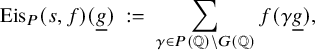(5.10) $$ \begin{align} \mathrm{{Eis}}_P(s, f)(\underline g) \ := \ \sum_{\gamma \in P(\mathbb{Q})\backslash G(\mathbb{Q})} f(\gamma \underline g), \end{align} $$

which is convergent if $\Re (s) \gg 0$ and has meromorphic continuation to the entire complex plane. This provides an intertwining operator

$$ \begin{align*}\mathrm{{Eis}}_P(s, \sigma\times \sigma^\prime) \ : \ I_P^G(s, \sigma \times \sigma^\prime) \ \longrightarrow \ \mathcal{C}^\infty\left(G(\mathbb{Q})\backslash G(\mathbb{A}), \omega_\infty^{-1}\right); \end{align*} $$

denote $\mathrm {{Eis}}_P(s, \sigma \times \sigma ^\prime )(f)$ simply as $\mathrm {{Eis}}_P(s, f).$ To construct a map in cohomology, one needs to evaluate at $s=-N/2,$ begging the question whether the Eisenstein series is holomorphic at $s=-N/2.$ For this, it is well known that one has to show that the constant term of the Eisenstein series is holomorphic at $s=-N/2.$

The constant term map

For the parabolic subgroup Q, the constant term map, denoted $\mathcal {F}^Q : \mathcal {C}^\infty (G(\mathbb {Q})\backslash G(\mathbb {A}), \omega _\infty ^{-1}) \to \mathcal {C}^\infty (M_Q(\mathbb {Q})U_Q(\mathbb {A})\backslash G(\mathbb {A}), \omega _\infty ^{-1}),$ is given by

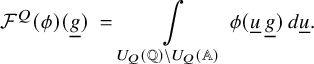(5.11) $$ \begin{align} \mathcal{F}^Q(\phi)(\underline g) \ = \ \int\limits_{U_Q(\mathbb{Q})\backslash U_Q(\mathbb{A})} \phi(\underline u \, \underline g)\, d\underline u. \end{align} $$

The choice of the global measure $d \underline {u}$

In the integrals defining the intertwining operator (5.9) and the constant term map (5.11), the choice of measure $d\underline u$ on $U_Q(\mathbb {A})$ needs to be fixed, where $U_Q = \mathrm {Res}_{F/\mathbb {Q}}(U_{Q_0})$ is the unipotent radical of the maximal parabolic subgroup Q; recall that $Q_0$ is the standard maximal parabolic subgroup of $\mathrm {{GL}}(N)$ corresponding to $N = n'+n$ . To begin, take the global measure ${}^L\!d\underline u$ on $U_Q(\mathbb {A}) = U_{Q_0}(\mathbb {A}_F)$ as a product over the coordinates of $U_{Q_0}$ of the additive measure $d\underline x$ on $\mathbb {A}_F$ , which in turn is a product $\prod _v dx_v$ of local additive measures $dx_v$ on $F_v^+$ ; for a finite place v normalise $dx_v$ by $\mathrm {vol}(\mathcal {O}_v) = 1$ , where $\mathcal {O}_v$ is the ring of integers of $F_v$ , and for an archimedean v take $dx_v$ as the Lebesgue measure on $\mathbb {C}.$ The notation ${}^L\!d\underline u$ is to suggest that this measure is well suited for the purposes of the analytic theory of L-functions. For the constant term map (5.11) to correspond to the restriction map in cohomology, the global measure should be normalized by asking $\mathrm {vol}(U_{Q_0}(F)\backslash U_{Q_0}(\mathbb {A}_F)) = 1;$ see Borel [3, Sect. 6]. Hence, consider the global measure on $U_Q(\mathbb {A}) = U_{Q_0}(\mathbb {A}_F)$ :

$$ \begin{align*}d\,\underline u \ := \ \frac{1}{\mathrm{vol}_{{}^L\!d\underline u}(U_{Q_0}(F)\backslash U_{Q_0}(\mathbb{A}_F))} \, {}^L\!d\underline u. \end{align*} $$

Of course, $\mathrm {vol}_{{}^L\!d\underline u}(U_{Q_0}(F)\backslash U_{Q_0}(\mathbb {A}_F)) = \mathrm {vol}_{d\underline x}(F\backslash \mathbb {A}_F)^{\dim (U_{Q_0})} = \mathrm {vol}_{d\underline x}(F\backslash \mathbb {A}_F)^{nn'}.$ Recall some classical algebraic number theory (see Tate [50, Sect. 4.1]) for the volume of $F\backslash \mathbb {A}_F.$ For the measure $d\underline x$ on $\mathbb {A}_F$ , the volume of a fundamental domain for the action of F on $\mathbb {A}_F$ is $|\delta _{F/\mathbb {Q}}|^{1/2}.$ If the set $\mathrm {{Hom}}(F,\mathbb {C})$ of complex embeddings of F is enumerated as, say, $\{\sigma _1,\dots , \sigma _{d_F} \}$ , and suppose $\{\omega _1,\dots ,\omega _{d_F}\}$ is a $\mathbb {Q}$ -basis of F, then the absolute discriminant of F is defined as $\delta _{F/\mathbb {Q}} = \det [\sigma _i(\omega _j)]^2.$ The square root of the absolute value of the discriminant, $|\delta _{F/\mathbb {Q}}|^{1/2},$ as an element of $\mathbb {R}^{\times }/\mathbb {Q}^{\times },$ is independent of the enumeration and the choice of basis. For the main theorem on L-values, the choice of measure can be changed by a nonzero rational number, which will still give the same rationality results and the reciprocity laws as in Theorem 5.16. Define the global measure on $U_Q(\mathbb {A}) = U_{Q_0}(\mathbb {A}_F)$ as

(5.12) $$ \begin{align} d \underline u \ := \ |\delta_{F/\mathbb{Q}}|^{- \tfrac{n n'}{2}} \, {}^L\!d\underline u. \end{align} $$

Theorem of Langlands on the constant term of an Eisenstein series

Theorem 5.13 (Langlands).

Let $f \in I_P^G(s, \sigma \times \sigma ').$

1. 1. In the non-self-associate cases ( $n \neq n'$ ), one has $\mathcal {F}^Q \circ \mathrm {{Eis}}_P(s, f) \ = \ T_{\mathrm {st}}(s, \sigma \times \sigma ')(f).$

2. 2. In the self-associate cases ( $n = n'$ and $P = Q$ ), one has $\mathcal {F}^P \circ \mathrm {{Eis}}_P(s, f) \ = \ f + T_{\mathrm {st}}(s, \sigma \times \sigma ')(f).$

Suppose $f = \otimes _v f_v$ is a pure tensor in $I_P^G(s, \sigma \otimes \sigma ')$ , and for $v \notin \mathrm {S}$ , suppose $f_v = f_v^0$ is the normalized spherical vector (normalized to take the value $1$ on the identity), and similarly, $\tilde f_v^0$ is such a vector in the v-th component of $I_Q^G(-s, \sigma ' \otimes \sigma )$ . Then from [47, Thm. 6.3.1], we have the fundamental analytic identity

(5.14) $$ \begin{align} \mathcal{F}^Q (\mathrm{{Eis}}_P(s, f)) \ = \ |\delta_{F/\mathbb{Q}}|^{- \tfrac{n n'}{2}} \, \frac{L^{\mathrm{S}}(s, \sigma \times \sigma^{\prime \mathrm v})}{L^{\mathrm{S}}(s+1, \sigma \times \sigma^{\prime \mathrm v})} \, \otimes_{v \notin \mathrm{S}} \tilde f_v^0 \otimes_{v \in \mathrm{S}} T_{\mathrm{st}}(s, \sigma_v \otimes \sigma^{\prime}_v)f_v. \end{align} $$

The proof of the main theorem on the arithmetic of special values of $L(s, \sigma \times \sigma ^{\prime \mathrm v})$ comes from seeing the contribution of this identity in cohomology.

Holomorphy of the Eisenstein series at the point of evaluation

Given weights $\mu \in X^+_{00}(T_n \times E)$ and $\mu ' \in X^+_{00}(T_{n'} \times E)$ and strongly-inner Hecke-summands $\sigma _f \in \mathrm {{Coh}}_{!!}(G_n, \mu )$ and $\sigma ^{\prime }_f \in \mathrm {{Coh}}_{!!}(G_{n'}, \mu '),$ recall then that ${}^\iota \sigma $ and ${}^\iota \sigma '$ are cuspidal automorphic representations of $G_n(\mathbb {A}) = \mathrm {{GL}}_n(\mathbb {A}_F)$ and $G_{n'}(\mathbb {A}) = \mathrm {{GL}}_{n'}(\mathbb {A}_F)$ for any $\iota : E \to \mathbb {C}$ . The pair $(\mu , \mu ')$ of weights is said to be on the right of the unitary axis if the abelian width is bounded above by the point of evaluation:

$$ \begin{align*}a(\mu,\mu') \leq -N/2. \end{align*} $$

To explain the terminology, it is clear from the definition of the cuspidal parameters (2.8), (2.9), and the archimedean representation (2.10) that ${}^\iota \sigma = {}^\iota \sigma _u \otimes |\!| \ |\!|^{-\mathbf {{w}}/2}$ for a unitary cuspidal representation ${}^\iota \sigma _u;$ similarly, ${}^\iota \sigma ' = {}^\iota \sigma ^{\prime }_u \otimes |\!| \ |\!|^{-\mathbf {{w}}'/2}.$ Hence, we have

$$ \begin{align*}L(s, {}^\iota\sigma \times {}^\iota\sigma^{\prime \mathrm{v}}) \ = \ L(s - a(\mu, \mu'), {}^\iota\sigma_u \times {}^\iota\sigma_u^{\prime \mathrm{v}}). \end{align*} $$

Now, suppose $(\mu , \mu ')$ is on the right of the unitary axis. Then for the L-value in the denominator of the right-hand side of (5.14) at the point of evaluation $s = - \tfrac {N}{2}$ , we have

$$ \begin{align*}L^{\mathrm{S}}(- \tfrac{N}{2}+1, {}^\iota\sigma \times {}^\iota\sigma^{\prime \mathrm{v}}) \ = \ L^{\mathrm{S}}(1 - \tfrac{N}{2} - a(\mu, \mu'), {}^\iota\sigma_u \times {}^\iota\sigma_u^{\prime \mathrm{v}}) \ \neq \ 0, \end{align*} $$

since $1 - \tfrac {N}{2} - a(\mu , \mu ') \geq 1,$ by a nonvanishing result for Rankin–Selberg L-functions recalled in [27, Thm. 7.1, (4)]. Of course, the nonvanishing of this L-value, the holomorphy of the Eisenstein series $\mathrm {{Eis}}_P(s,f)$ or of its constant term are all intimately linked. We have the following well-known result ([39] and [28, Chap. IV § 5]).

Theorem 5.15. Suppose we are given weights $\mu \in X^+_{00}(T_n \times E)$ and $\mu ' \in X^+_{00}(T_{n'} \times E),$ strongly-inner Hecke-summands $\sigma _f \in \mathrm {{Coh}}_{!!}(G_n, \mu )$ and $\sigma ^{\prime }_f \in \mathrm {{Coh}}_{!!}(G_{n'}, \mu '),$ and an $\iota : E \to \mathbb {C}.$ Assume that $(\mu , \mu ')$ is on the right of the unitary axis. Then $\mathrm {{Eis}}_P(s,f)$ is holomorphic at $s = -N/2$ , unless we are in the exceptional case $n=n^\prime $ and ${}^\iota \sigma ^\prime = {}^\iota \sigma \otimes | \ |^{-n-1}.$

The poles on the right of the unitary axis are simple and contribute to the residual spectrum [28], and then the assertion follows from [39]. The exceptional case exactly corresponds to when the numerator of of the right-hand side of (5.14) at the point of evaluation is a pole at $1$ , that is, when $L(- \tfrac {N}{2} - a(\mu , \mu '), {}^\iota \sigma _u \times {}^\iota \sigma _u^{\prime \mathrm {v}})$ is a pole at $1$ , which is possible only when $n=n^\prime $ and ${}^\iota \sigma ^\prime = {}^\iota \sigma \otimes |\!| \ |\!|^{-n-1}.$ To parse this further: If ${}^\iota \sigma ^\prime = {}^\iota \sigma \otimes |\!| \ |\!|^r$ for any integer r, then $\mu ' = \mu -r$ . Then the cuspidal parameters for $\mu '$ and $\mu $ are related thus: $\alpha ^{\prime v}_i = \alpha ^v_i+r, \ \beta ^{\prime v}_i = \beta ^v_i+r;$ hence, the cuspidal width $\ell (\mu , \mu ') = 0.$ For the main theorem on L-values, we will assume the conditions imposed by the combinatorial lemma (Lemma 3.16), and in particular, we will have $\ell (\mu ,\mu ') \geq 2$ to guarantee at least two critical values. Hence, the exceptional case will not be relevant to us.

5.3 The main theorem on L-values

5.3.1 Statement of the main theorem

Theorem 5.16. Let n and $n'$ be two positive integers. Let F be a totally imaginary field, and E a finite Galois extension of $\mathbb {Q}$ that contains a copy of F. Consider strongly-pure weights $\mu \in X^+_{00}(T_n \times E)$ and $\mu ' \in X^+_{00}(T_{n'} \times E).$ Let $\sigma _f \in \mathrm {{Coh}}_{!!}(G_n, \mu )$ and $\sigma ^{\prime }_f \in \mathrm {{Coh}}_{!!}(G_{n'}, \mu ')$ be strongly-inner Hecke-summands, and assume that E is large enough to contain all the Hecke-eigenvalues for $\sigma _f $ and $\sigma ^{\prime }_f.$ Let $\iota : E \to \mathbb {C}$ be an embedding. Recall then that ${}^\iota \sigma $ and ${}^\iota \sigma '$ are cuspidal automorphic representations of $G_n(\mathbb {A}) = \mathrm {{GL}}_n(\mathbb {A}_F)$ and $G_{n'}(\mathbb {A}) = \mathrm {{GL}}_{n'}(\mathbb {A}_F)$ , respectively. Put $N = n+n'.$

Suppose that $m \in \tfrac {N}{2} + \mathbb {Z}$ is such that both m and $1+m$ are critical for the Rankin–Selberg L-function $L(s, {}^\iota \sigma \times {}^\iota \sigma ^{\prime \mathrm {v}}).$

1. 1. If for some $\iota $ , $L(1 + m, {}^\iota \sigma \times {}^\iota \sigma ^{\prime \mathrm {v}}) = 0$ , then $1+m -a(\mu ,\mu ') = \tfrac 12$ and

   $$ \begin{align*}L(1 + m, {}^\iota\sigma \times {}^\iota\sigma^{\prime \mathrm{v}}) \ = \ L(\tfrac12, {}^\iota\sigma_u \times {}^\iota\sigma^{\prime \mathrm{v}}_u) = 0 \end{align*} $$
   is the central critical value. Furthermore, $L(1+m, {}^\iota \sigma \times {}^\iota \sigma ^{\prime \mathrm {v}}) = 0$ for every $\iota .$

2. 2. Assume F is in the CM-case. Suppose that $L(1 +m, {}^\iota \sigma \times {}^\iota \sigma ^{\prime \mathrm {v}}) \neq 0$ . Then we have

   $$ \begin{align*}|\delta_{F/\mathbb{Q}}|^{- \tfrac{n n'}{2}} \, \frac{L(m, {}^\iota\sigma \times {}^\iota\sigma^{\prime \mathrm{v}})}{L(1+m, {}^\iota\sigma \times {}^\iota\sigma^{\prime \mathrm{v}})} \ \in \ \iota(E). \end{align*} $$
   Since $L(m, {}^\iota \sigma \times {}^\iota \sigma ^{\prime \mathrm {v}}) = L(-N/2, {}^\iota \sigma (N/2+m) \times {}^\iota \sigma ^{\prime \mathrm {v}})$ , the pair $(\mu -N/2-m, \mu ')$ of weights satisfies Lemma 3.16 giving a balanced Kostant representative $w \in W^P$ . Let $w' \in W^Q$ be determined by Lemma 5.1. Furthermore, for any $\gamma \in \mathrm {{Gal}}(\bar {\mathbb {Q}}/\mathbb {Q})$ , we have
   $$ \begin{align*}\gamma\left( |\delta_{F/\mathbb{Q}}|^{- \tfrac{n n'}{2}} \, \frac{L(m, {}^\iota\sigma \times {}^\iota\sigma^{\prime \mathrm{v}})}{L(1+m, {}^\iota\sigma \times {}^\iota\sigma^{\prime \mathrm{v}})} \right) \ = \ \varepsilon_{\iota, w}(\gamma) \cdot \varepsilon_{\iota, w'}(\gamma) \cdot |\delta_{F/\mathbb{Q}}|^{- \tfrac{n n'}{2}} \, \frac{L(m, {}^{\gamma\circ\iota}\sigma \times {}^{\gamma \circ\iota} \sigma^{\prime \mathrm{v}})}{L(1+m, {}^{\gamma \circ \iota}\sigma \times {}^{\gamma \circ\iota}\sigma^{\prime \mathrm{v}})}. \end{align*} $$

3. 3. Assume F is in the TR-case. Then $nn'$ is even. Suppose that $L(1 +m, {}^\iota \sigma \times {}^\iota \sigma ^{\prime \mathrm {v}}) \neq 0$ . Then we have

   $$ \begin{align*}\frac{L(m, {}^\iota\sigma \times {}^\iota\sigma^{\prime \mathrm{v}})}{L(1+m, {}^\iota\sigma \times {}^\iota\sigma^{\prime \mathrm{v}})} \ \in \ \iota(E). \end{align*} $$
   Furthermore, for any $\gamma \in \mathrm {{Gal}}(\bar {\mathbb {Q}}/\mathbb {Q})$ , we have
   $$ \begin{align*}\gamma\left( \frac{L(m, {}^\iota\sigma \times {}^\iota\sigma^{\prime \mathrm{v}})}{L(1+m, {}^\iota\sigma \times {}^\iota\sigma^{\prime \mathrm{v}})} \right) \ = \ \frac{L(m, {}^{\gamma\circ\iota}\sigma \times {}^{\gamma \circ\iota} \sigma^{\prime \mathrm{v}})}{L(1+m, {}^{\gamma \circ \iota}\sigma \times {}^{\gamma \circ\iota}\sigma^{\prime \mathrm{v}})}. \end{align*} $$

As mentioned in the introduction, statement (1) is originally due to Mœglin [38, Sect. 5]; our proof below is independent of [38]. More generally, the assertion on the vanishing of the central critical value is a special case of Deligne’s conjecture [8, Conj. 2.7, (ii)] based on a suggestion of Benedict Gross that the order of vanishing at a critical point is independent of the embedding $\iota $ .

5.3.2 Proof of the main theorem

Finiteness of the relevant L-values

The paragraph after Theorem 5.15 says that if $L(s, {}^\iota \sigma \otimes \times {}^\iota \sigma ^{\prime \mathrm {v}})$ has a pole at $m \in \tfrac {N}{2} + \mathbb {Z}$ , then the cuspidal width $\ell (\mu ,\mu ') = 0$ ; a situation which is ruled out by the hypothesis that requires two critical points. Hence, all the L-values under consideration are finite – a fact that will be used without further comment.

It suffices to prove Theorem 5.16 for the point of evaluation $m = -N/2$

If the theorem is known for the critical points $s = -\tfrac {N}{2}$ and $1-\tfrac {N}{2}$ and for all possible $\mu $ , $\mu '$ , $\sigma _f$ , $\sigma ^{\prime }_f$ , then one can deduce the theorem for any pair of successive critical points $m, \, m+1$ for a given $\sigma _f$ and $\sigma ^{\prime }_f$ . This follows from using Tate-twists (Section 2.4.1) and the combinatorial lemma (Lemma 3.16). Take any integer r and replace $\mu $ by and $\sigma _f$ by $\sigma _f(r).$ Note that ${}^\iota (\sigma _f(r)) = {}^\iota \sigma _f \otimes |\!|\ |\!|^r.$ The condition that $-\tfrac {N}{2}$ and $1-\tfrac {N}{2}$ are critical for $L(s, {}^\iota \sigma \otimes |\!|\ |\!|^r \times {}^\iota \sigma ^{\prime \mathrm {v}}) = L(s +r, {}^\iota \sigma \otimes \times {}^\iota \sigma ^{\prime \mathrm {v}})$ , after the combinatorial lemma, bounds the abelian width by the cuspidal width as in (2) of Lemma 3.16. Now, the crucial point is that, whereas for the abelian width one has , but for the cuspidal width one has independence of r in as much as . This bounds the possible twisting integers r above and below as

$$ \begin{align*}- \frac{N}{2} + 1 - \frac{\ell(\mu,\mu')}{2} - a(\mu, \mu') \ \leq \ -r \ \leq \ - \frac{N}{2} -1 + \frac{\ell(\mu,\mu')}{2} - a(\mu, \mu'). \end{align*} $$

As r ranges over this set, using the critical set described in Proposition 3.12, one sees that

$$ \begin{align*}\frac{L(- \tfrac{N}{2}, {}^\iota\sigma(r) \times {}^\iota\sigma^{\prime \mathrm{v}})}{L(1- \tfrac{N}{2}, {}^\iota\sigma(r) \times {}^\iota\sigma^{\prime \mathrm{v}})} \ = \ \frac{L(r - \tfrac{N}{2}, {}^\iota\sigma \times {}^\iota\sigma^{\prime \mathrm{v}})}{L(r+1- \tfrac{N}{2}, {}^\iota\sigma \times {}^\iota\sigma^{\prime \mathrm{v}})} \end{align*} $$

runs over the set of all successive pairs of critical points; no more and no less! The number of possible r is $\ell (\mu ,\mu ')-1$ , which is exactly the number of pairs of successive critical points.

Being on the right versus on the left of the unitary axis

Suppose that $(\mu ,\mu ')$ is on the right of the unitary axis: $a(\mu ,\mu ') \leq -\tfrac {N}{2}.$ Then (1) is vacuously true since $L(1 - \tfrac {N}{2}, {}^\iota \sigma \times {}^\iota \sigma ^{\prime \mathrm {v}}) = L(1 - \tfrac {N}{2} - a(\mu ,\mu '), {}^\iota \sigma _u \times {}^\iota \sigma ^{\prime \mathrm {v}}_u) \neq 0$ by a well-known nonvanishing result for Rankin–Selberg L-functions as already mentioned before. Next, recall that the Eisenstein series $\mathrm {{Eis}}_P(s,f)$ is holomorphic at $s = -\tfrac {N}{2}$ , and at this point of evaluation, (2) and (3) will be proved below. Granting this, suppose, on the other hand, that $(\mu , \mu ')$ is on the left of the unitary axis; that is, $a(\mu ,\mu ')> -\tfrac {N}{2}.$ Then, $a(\mu ',\mu ) < \tfrac {N}{2};$ that is, $(\mu ',\mu )$ is on the right of the unitary axis for the point of evaluation is $\tfrac {N}{2}$ , so we get the holomorphy of $\mathrm {{Eis}}_Q(s,f)$ at $s = \tfrac {N}{2}$ and whence statement (2) for $L(s, {}^\iota \sigma ' \times {}^\iota \sigma ^{\mathrm {v}})$ and for $s = \tfrac {N}{2}.$ And as above, (1) is in fact vacuously true because $L(1+\tfrac {N}{2}, {}^\iota \sigma ' \times {}^\iota \sigma ^{\mathrm {v}}) = L(1+\tfrac {N}{2} - a(\mu ',\mu ), {}^\iota \sigma ^{\prime }_u \times {}^\iota \sigma ^{\mathrm {v}}_u) \neq 0.$ Statement (2) for this situation says

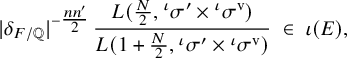$$ \begin{align*}|\delta_{F/\mathbb{Q}}|^{- \tfrac{n n'}{2}} \, \frac{L(\tfrac{N}{2}, {}^\iota\sigma' \times {}^\iota\sigma^{\mathrm{v}})}{L(1+\tfrac{N}{2}, {}^\iota\sigma' \times {}^\iota\sigma^{\mathrm{v}})} \ \in \ \iota(E), \end{align*} $$

where the L-value in the denominator is not zero. Suppose the L-value in the numerator is $0$ (which can happen in the special case $\tfrac {N}{2} - a(\mu ',\mu ) = \tfrac 12$ ). Then the Galois equivariance in (2) implies that $L(\tfrac {N}{2}, {}^\iota \sigma ' \times {}^\iota \sigma ^{\mathrm {v}}) = 0$ for every $\iota .$ Applying the functional equation ([27, (3), Thm. 7.1]) to the above ratio of L-values, we get

$$ \begin{align*}|\delta_{F/\mathbb{Q}}|^{- \tfrac{n n'}{2}} \cdot \frac{\varepsilon(\tfrac{N}{2}, {}^\iota\sigma' \times {}^\iota\sigma^{\mathrm{v}})} {\varepsilon(1+\tfrac{N}{2}, {}^\iota\sigma' \times {}^\iota\sigma^{\mathrm{v}})} \cdot \frac{L(1- \tfrac{N}{2}, {}^\iota\sigma \times {}^\iota\sigma^{\prime \mathrm{v}})} {L(- \tfrac{N}{2}, {}^\iota\sigma \times {}^\iota\sigma^{\prime \mathrm{v}})} \ \in \ \iota(E). \end{align*} $$

For brevity, let $\tau := {}^\iota \sigma ' \times {}^\iota \sigma ^{\mathrm {v}}$ . The global epsilon-factor is a product of local factors as $\varepsilon (s, \tau ) = \prod _v \varepsilon (s, \tau _v, \psi _v)$ , where we have fixed an additive character $\psi : F \backslash \mathbb {A}_F \to \mathbb {C}^{\times }.$ (See, for example, [47, Sect. 10.1].) At a non-archimedean place v, the local factor has the form $\varepsilon (s, \tau _v, \psi _v) = W(\tau _v) q_v^{(1/2 - s)(c(\tau _v)+c(\psi _v))}$ , where $W(\tau _v)$ is the local root number, $q_v$ the cardinality of the residue field of $F_v$ , and $c(\tau _v)$ and $c(\psi _v)$ are integers defined to be the conductoral exponents of the respective data; it follows that $\varepsilon (N/2, \tau _v, \psi _v)/\varepsilon (1+N/2, \tau _v, \psi _v)$ is an integral power of $q_v$ . At an archimedean place, it follows from [35, (4.7)] that the local factor is a constant, and hence the ratio is $1$ . Whence, $\varepsilon (\tfrac {N}{2}, {}^\iota \sigma ' \times {}^\iota \sigma ^{\mathrm {v}})/\varepsilon (1+\tfrac {N}{2}, {}^\iota \sigma ' \times {}^\iota \sigma ^{\mathrm {v}})$ is a nonzero integer, from which it follows that

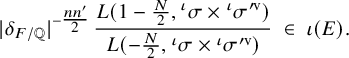(5.17) $$ \begin{align} |\delta_{F/\mathbb{Q}}|^{- \tfrac{n n'}{2}} \, \frac{L(1- \tfrac{N}{2}, {}^\iota\sigma \times {}^\iota\sigma^{\prime \mathrm{v}})} {L(- \tfrac{N}{2}, {}^\iota\sigma \times {}^\iota\sigma^{\prime \mathrm{v}})} \ \in \ \iota(E). \end{align} $$

From the functional equation, it is clear that $ L(1- \tfrac {N}{2}, {}^\iota \sigma \times {}^\iota \sigma ^{\prime \mathrm {v}}) = 0 \iff L(\tfrac {N}{2}, {}^\iota \sigma ' \times {}^\iota \sigma ^{\mathrm {v}}) = 0, $ proving (1) when $(\mu , \mu ')$ is on the left of the unitary axis. If $L(1- \tfrac {N}{2}, {}^\iota \sigma \times {}^\iota \sigma ^{\prime \mathrm {v}}) \neq 0$ , then taking reciprocal of the ratio on the left-hand side of (5.17), (2) will follow when $(\mu , \mu ')$ is on the left of the unitary axis. (See also [27, Sect. 7.3.2.5] for a slightly different way to argue this point if $(\mu , \mu ')$ is on the left of the unitary axis.) The discussion is the same for (3).

Proof of the rationality result

After the above reductions, it suffices to prove (2) and (3) of Theorem 5.16 when $(\mu ,\mu ')$ is on the right of the unitary axis and for $m = -N/2.$ This involves Eisenstein cohomology. Assume henceforth that $(\mu ,\mu ')$ is on the right of the unitary axis. For now, F is any totally imaginary field (either CM or TR). By Theorem 5.6, the subspace $\mathfrak {I}^b(\sigma _f, \sigma _f^{\prime })$ , which is the image of global cohomology in the $2{\mathrm k}$ -dimensional E-vector space $I^{\mathrm {S}}_b(\sigma _f,\sigma _f^{\prime })_{P,w} \oplus I^{\mathrm {S}}_b(\sigma ^{\prime }_f(n),\sigma _f(-n'))_{Q,w'}$ , is a ${\mathrm k}$ -dimensional E-subspace, and furthermore, from the proof of that theorem, we get an intertwining operator $T_{\mathrm {Eis}}(\sigma , \sigma ')$ defined over E such that in the non-self-associate case ( $n\neq n'$ ), we have

$$ \begin{align*}\mathfrak{I}^b(\sigma_f, \sigma_f^{\prime}) \ = \ \left\{ \left(\xi, \, T_{\mathrm{Eis}}(\sigma, \sigma')(\xi)\right) \ | \ \xi \in I^{\mathrm{S}}_b(\sigma_f,\sigma_f^{\prime})_{P,w} \right\}, \end{align*} $$

and in the self-associate case, we will have

$$ \begin{align*}\mathfrak{I}^b(\sigma_f, \sigma_f^{\prime}) \ = \ \left\{ \left(\xi, \, \xi+ T_{\mathrm{Eis}}(\sigma, \sigma')(\xi)\right) \ | \ \xi \in I^{\mathrm{S}}_b(\sigma_f,\sigma_f^{\prime})_{P,w} \right\}. \end{align*} $$

The idea of the proof is to take $T_{\mathrm {Eis}}(\sigma , \sigma ')$ to a transcendental level, use the constant term theorem which gives L-values, and then descend back to an arithmetic level, giving a rationality result for the said L-values. Take an $\iota : E \to \mathbb {C}$ , and consider $T_{\mathrm {Eis}}(\sigma , \sigma ') \otimes _{E, \iota } \mathbb {C}$ . We have

$$ \begin{align*}\mathfrak{I}^b({}^\iota\!\sigma_f, {}^\iota\!\sigma_f^{\prime}) \ = \ \left\{ \left(\xi \, , \, T_{\mathrm{st}}(-\tfrac{N}{2}, {}^\iota\!\sigma \otimes {}^\iota\!\sigma')^{\bullet}\xi \right) \ : \ \xi \in I^{\mathrm{S}}_b({}^\iota\!\sigma_f, {}^\iota\!\sigma_f^{\prime})_{P, {}^\iota\!w} \right\} \end{align*} $$

in the non-self-associate case, and with analogous modification for the self-associate case. Here, $T_{\mathrm {st}}(-\tfrac {N}{2}, {}^\iota \!\sigma \otimes {}^\iota \!\sigma ')^{\bullet }$ is the map induced by the standard intertwining operator in relative Lie algebra cohomology. For brevity, let $\underline {\sigma } = \sigma \times \sigma '$ . The global operator $T_{\mathrm {st}}(-\tfrac {N}{2}, {}^\iota \!\underline {\sigma })^{\bullet }$ factors into local standard intertwining operators. The discussion in [27, Sect. 7.3.2.1] involving rationality properties of local standard intertwining operators at finite places goes through verbatim in our situation. (See also my paper [43] where this discussion is situated in a broader context.) We have for $T_{\mathrm {Eis}}(\sigma , \sigma ') \otimes _{E, \iota } \mathbb {C}$ the following expression (the exact analogue of [27, (7.38)]):

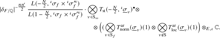(5.18) $$ \begin{align} |\delta_{F/\mathbb{Q}}|^{- \tfrac{n n'}{2}} \, \frac{L (-\tfrac{N}{2}, {}^\iota\sigma_f \times {}^\iota\sigma_f^{\prime \mathrm v})} {L (1-\tfrac{N}{2}, {}^\iota\sigma_f \times {}^\iota\sigma_f^{\prime \mathrm v})} \, \cdot &\bigotimes_{v\in {\mathrm{S}}_\infty} T_{\mathrm{st}}(-\tfrac{N}{2}, {}^\iota\underline{\sigma}_v)^{\bullet} \otimes\notag \\ &\quad \otimes \Big((\bigotimes_{v \in \mathrm{S}_f} T^{\mathrm{ar}}_{\mathrm{norm}}( \underline{\sigma}_v)(1) \otimes \bigotimes_{v \not\in \mathrm{S}}T^{\mathrm{ar}}_{\mathrm{loc}}( \underline{\sigma}_v)(1) \Big)\otimes_{E,\iota}\mathbb{C}. \end{align} $$

The local operators $T^{\mathrm {ar}}_{\mathrm {norm}}( \underline {\sigma }_v)(1)$ and $T^{\mathrm {ar}}_{\mathrm {loc}}( \underline {\sigma }_v)(1)$ are exactly as in loc.cit.; the point of immediate interest for us being that they are defined over E. For the archimedean component $T_{\mathrm {st}}(-\tfrac {N}{2}, {}^\iota \underline {\sigma }_v)^{\bullet }$ , we use Proposition 4.32 to get for $T_{\mathrm {Eis}}(\sigma , \sigma ') \otimes _{E, \iota } \mathbb {C}$ the following expression involving values of the completed L-function:

(5.19) $$ \begin{align} |\delta_{F/\mathbb{Q}}|^{- \tfrac{n n'}{2}} \, \frac{L (-\tfrac{N}{2}, {}^\iota\sigma \times {}^\iota\sigma^{\prime {\mathrm v}})} {L (1-\tfrac{N}{2}, {}^\iota\sigma \times {}^\iota\sigma^{\prime {\mathrm v}})} \, \cdot \, \Big((\bigotimes_{v \in \mathrm{S}_f} T^{\mathrm{ar}}_{\mathrm{norm}}( \underline{\sigma}_v)(1) \otimes \bigotimes_{v \not\in \mathrm{S}}T^{\mathrm{ar}}_{\mathrm{loc}}( \underline{\sigma}_v)(1) \Big)\otimes_{E,\iota}\mathbb{C}. \end{align} $$

We conclude that the complex number $|\delta _{F/\mathbb {Q}}|^{- \tfrac {n n'}{2}} \, L (-\tfrac {N}{2}, {}^\iota \sigma \times {}^\iota \sigma ^{\prime \mathrm v})/L (1-\tfrac {N}{2}, {}^\iota \sigma \times {}^\iota \sigma ^{\prime \mathrm v})$ is in $\iota (E).$ When F is in case-TR, existence of a critical point implies $nn'$ is even (Corollary 3.14), which forces $|\delta _{F/\mathbb {Q}}|^{- \tfrac {n n'}{2}} \in \mathbb {Q}^{\times }.$

Proof of reciprocity

For Galois equivariance, apply $\gamma \in \mathrm {{Gal}}(\bar {\mathbb {Q}}/\mathbb {Q})$ , to the objects and maps in the first paragraph of Section 5.2.2, while keeping in mind the behaviour of cohomology groups as Hecke modules under changing the base field E. Assume now that F is a totally imaginary field in the CM-case. The claim is that Galois-action and Eisenstein operator $T_{\mathrm {Eis}}(\sigma , \sigma ')$ intertwine as

(5.20) $$ \begin{align} (1 \otimes \gamma) \circ \left(T_{\mathrm{Eis}}(\sigma, \sigma') \otimes_{E,\iota} \bar{\mathbb{Q}} \right) \ = \ \varepsilon_{\iota, w}(\gamma) \cdot \varepsilon_{\iota, w'}(\gamma) \cdot T_{\mathrm{Eis}}(\sigma, \sigma') \otimes_{E, \gamma \circ \iota} \bar{\mathbb{Q}}. \end{align} $$

From this claim and (5.19), the reciprocity law will follow. To prove this claim, take $n \neq n'$ (the reader can easily modify the argument for the self-associate case) and consider the following diagram

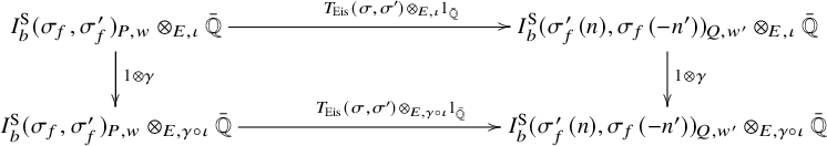
The left (resp., right) vertical arrow introduces the signature $\varepsilon _{\iota , w}(\gamma )$ (resp., $\varepsilon _{\iota , w'}(\gamma )$ ), and the diagram commutes up to the product of these two signatures. For the left vertical arrow, recall from 5.1.3 that the induced module $I^{\mathrm {S}}_b(\sigma _f,\sigma _f^{\prime })_{P,w}$ appears in boundary cohomology as ${{}^{\mathrm {a}}\mathrm {Ind}}_{P(\mathbb {A}_f)}^{G(\mathbb {A}_f)} \left (H^{b_n^F+b_{n'}^F}(\mathcal {S}^{M_P}, \widetilde {\mathcal {M}}_{w \cdot \lambda , E})(\sigma _f \times \sigma ^{\prime }_f) \right )^{K_f}.$ Hence, $I^{\mathrm {S}}_b(\sigma _f,\sigma _f^{\prime })_{P,w} \otimes _{E,\iota } \bar {\mathbb {Q}}$ appears as a Hecke-summand in ${{}^{\mathrm {a}}\mathrm {Ind}}_{P(\mathbb {A}_f)}^{G(\mathbb {A}_f)} \left (H^{b_n^F+b_{n'}^F}(\mathcal {S}^{M_P}, \widetilde {\mathcal {M}}_{{}^\iota \!w \cdot {}^\iota \! \lambda , \bar {\mathbb {Q}}})\right )$ . Recall from (2.30) that $\gamma $ maps the the highest weight vector of the coefficient system $\mathcal {M}_{{}^\iota \!w \cdot {}^\iota \! \lambda , \bar {\mathbb {Q}}}$ to $\varepsilon _{\iota , w}(\gamma )$ times the highest weight vector of the coefficient system $\mathcal {M}_{{}^{\gamma \circ \iota }\!w \cdot {}^{\gamma \circ \iota }\! \lambda , \bar {\mathbb {Q}}}$ explaining the homothety by $\varepsilon _{\iota , w}(\gamma )$ in the left vertical arrow. Similarly, the induced module $I^{\mathrm {S}}_b(\sigma ^{\prime }_f(n),\sigma _f(-n'))_{Q,w'} \otimes _{E,\iota } \bar {\mathbb {Q}} $ appears in ${{}^{\mathrm {a}}\mathrm {Ind}}_{P(\mathbb {A}_f)}^{G(\mathbb {A}_f)} \left (H^{b_n^F+b_{n'}^F}(\mathcal {S}^{M_P}, \widetilde {\mathcal {M}}_{{}^\iota \!w' \cdot {}^\iota \! \lambda , \bar {\mathbb {Q}}})\right )$ for $w'$ related to w by Lemma 5.1. Hence, in the right vertical arrow, one gets a homothety by $\varepsilon _{\iota , w'}(\gamma )$ . Hence the claim, and whence the reciprocity law.

If the totally imaginary field F is in case CM, then the proof of (2) is complete. In case of TR, the rationality and the Galois-equivariance, as will be now shown, will simplify to give the corresponding statements in (3). Assume now that F is TR, and that $F_1$ is the maximal totally real subfield of F. Existence of a critical point implies $nn'$ is even by Corollary 3.14; hence, $|\delta _{F/\mathbb {Q}}|^{- \tfrac {n n'}{2}} \in \mathbb {Q}^{\times }$ , and so we may absorb it into $\iota (E)$ and ignore it from the Galois-equivariance. The simplified Galois equivariance in (3) follows from the following:

Lemma 5.21. Suppose that F is TR. Then $\varepsilon _{\iota , w}(\gamma ) = 1 = \varepsilon _{\iota , w'}(\gamma ).$

Proof. Recall the notations from 2.3.5: $\Sigma _{F_1} = \{\nu _1,\dots ,\nu _{d_1}\}$ , $\varrho : \Sigma _F \to \Sigma _{F_1}$ , $k = 2k_1,$ and $\varrho ^{-1}(\nu _j) = \{\eta _{j1}, \bar {\eta }_{j1},\dots , \eta _{jk_1} \bar {\eta }_{jk_1}\}.$ Since $\mu $ and $\mu '$ are strongly-pure weights that are the base-change from weight over $F_1$ , the Kostant representative w (and then so also $w'$ ) has the property that all the constituents $w^{\eta },$ as $\eta $ varies over $\varrho ^{-1}(\nu _j),$ are copies of the same element of $\mathfrak {S}_N$ –the Weyl group of $\mathrm {{GL}}_N$ ; in particular, since w is balanced, $l(w^\eta ) + l(w^{\bar {\eta }}) = nn'$ and $l(w^\eta ) = l(w^{\bar {\eta }})$ since $\eta $ and $\bar {\eta }$ have the same restriction to $F_1$ ; hence, $l(w^\eta ) = nn'/2$ . Recalling the notations from Section 2.7, consider the wedge product

$$ \begin{align*}e_{\Phi_{^\iota \! w, [\nu_j]}}^{*} \ := \ e_{\Phi_{^\iota \! w^{\eta_{j1}}}}^{*} \wedge e_{\Phi_{^\iota \! w^{\bar{\eta}_{j1}}}}^{*} \wedge \cdots \wedge e_{\Phi_{^\iota \! w^{\eta_{jk_1}}}}^{*} \wedge e_{\Phi_{^\iota \! w^{\bar{\eta}_{jk_1}}}}^{*}. \end{align*} $$

All the individual factors such as $e_{\Phi _{^\iota \! w^{\eta _{ji}}}}^{*}$ or $e_{\Phi _{^\iota \! w^{\bar {\eta }_{ji}}}}^{*}$ are identical and have degree $nn'/2$ . Hence, the total degree of $e_{\Phi _{^\iota \! w, [\nu _j]}}^{*}$ is $nn'/2 \cdot k = nn'k_1.$ From (2.26), one gets

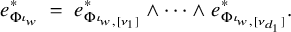$$ \begin{align*}e_{\Phi_{^\iota \! w}}^{*} \ = \ e_{\Phi_{^\iota \! w, [\nu_1]}}^{*} \wedge \cdots \wedge e_{\Phi_{^\iota \! w, [\nu_{d_1}]}}^{*}. \end{align*} $$

Denote the action of $\gamma $ on $\Sigma _{F_1},$ for the ordering fixed above, as $\pi _{F_1}(\gamma ),$ and let $\varepsilon _{F_1}(\gamma )$ denote its signature. Then one has

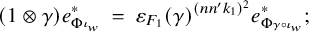$$ \begin{align*}(1 \otimes \gamma) e_{\Phi_{^\iota \! w}}^{*} \ = \ \varepsilon_{F_1}(\gamma)^{(nn'k_1)^2} e_{\Phi_{^{\gamma \circ \iota} \! w}}^{*}; \end{align*} $$

from Definition 2.29, one has $\varepsilon _{\iota , w}(\gamma ) = \varepsilon _{F_1}(\gamma )^{(nn'k_1)^2} = 1$ since $nn'k_1 \equiv 0 \ \pmod {2}.$ Similarly, $\varepsilon _{\iota , w'}(\gamma ) = 1.$

This concludes the proof of Theorem 5.16.

5.4 Compatibility with Deligne’s Conjecture

5.4.1 Statement of Deligne’s Conjecture

In this subsection, Deligne’s celebrated conjecture on the special values of motivic L-functions is formulated for the ratios of successive successive critical L-values for Rankin–Selberg L-functions. The notations of [8] will be freely used; a motive M over $\mathbb {Q}$ with coefficients in a field E will be thought in terms of its Betti, de Rham and $\ell $ -adic realizations. Attached to a critical motive M are its periods $c^\pm (M) \in (E \otimes \mathbb {C})^{\times }$ as in loc.cit., that are well defined in $(E \otimes \mathbb {C})^{\times }/E^{\times }.$ We begin with a relation between the two periods over a totally imaginary base field F. Recall from the introduction that if F is in the CM-case, then $F_1$ is its maximal CM subfield which is totally imaginary quadratic over the totally real subfield $F_1$ ; suppose $F_1 = F_0(\sqrt {D})$ for a totally negative $D \in F_0$ . Then define

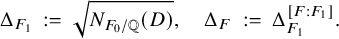$$ \begin{align*}\Delta_{F_1} \ := \ \sqrt{N_{F_0/\mathbb{Q}}(D)}, \quad \Delta_F \ := \ \Delta_{F_1}^{[F:F_1]}. \end{align*} $$

If F is in the TR-case, then $F_1 = F_0$ is the maximal totally real subfield. Then define

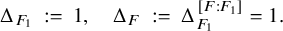$$ \begin{align*}\Delta_{F_1} \ := \ 1, \quad \Delta_F \ := \ \Delta_{F_1}^{[F:F_1]} = 1. \end{align*} $$

The following result is stated in my paper with Deligne; see [9, Thm. 3.4.2]:

Proposition 5.22. Let $M_0$ be a pure motive of rank n over a totally imaginary number field F with coefficients in a number field E. Put $M = \mathrm {Res}_{F/\mathbb {Q}}(M_0),$ and suppose that M has no middle Hodge type. Let $c^\pm (M)$ be the periods defined in [8]. Then

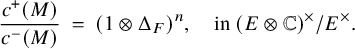$$ \begin{align*}\frac{c^+(M)}{c^-(M)} \ = \ (1 \otimes \Delta_F)^n, \quad \mbox{in } (E \otimes \mathbb{C})^{\times}/ E^{\times}. \end{align*} $$

Under the identification $E \otimes \mathbb {C} = \prod _{\iota : E \to \mathbb {C}} \mathbb {C}$ , the element $1 \otimes \Delta _F$ is $\pm 1$ in each component of $(E \otimes \mathbb {C})^{\times }/ E^{\times }$ , since its square is trivial. Based on Proposition 5.22, Deligne’s conjecture [8] for the ratios of successive critical values of the completed L-function of M may be stated as the following:

Conjecture 5.23 (Deligne).

Let $M_0$ be a pure motive of rank n over a totally imaginary F with coefficients in E. Put $M = \mathrm {Res}_{F/\mathbb {Q}}(M_0),$ and suppose that M has no middle Hodge type. For $\iota : E \to \mathbb {C}$ , let $L(s, \iota , M)$ denote the completed L-function attached to $(M, \iota ).$ Put $L(s,M) = \{L(s, \iota , M)\}_{\iota : E \to \mathbb {C}}$ for the array of L-functions taking values in $E \otimes \mathbb {C}.$ Suppose m and $m+1$ are critical integers for $L(s,M)$ , and assuming that $L(m+1,M) \neq 0$ , we have

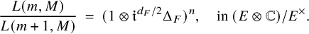$$ \begin{align*}\frac{L(m,M)}{L(m+1,M)} \ = \ (1\otimes {\mathfrak{i}}^{d_F/2} \Delta_F)^n, \quad \mbox{in } (E \otimes \mathbb{C})/ E^{\times}. \end{align*} $$

A word of explanation is in order since, in [8], Deligne formulated his conjecture for critical values of $L_f(s,M)$ – the finite-part of the L-function attached to $M.$ From Conjecture 2.8 and (5.1.8) of [8] for M as above, one can deduce

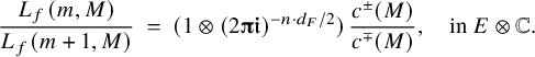
Knowing the L-factor at infinity, one has hence, for the completed L-function, one can deduce

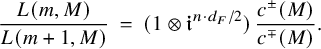(5.24) $$ \begin{align} \frac{L(m, M)}{L(m+1, M)} \ = \ (1 \otimes {\mathfrak{i}}^{n\cdot d_F/2}) \, \frac{c^\pm(M)}{c^\mp(M)}. \end{align} $$

It is clear now that (5.24) and Proposition 5.22 give Conjecture 5.23.

There is conjectural correspondence between $\sigma _f \in \mathrm {{Coh}}_{!!}(\mathrm {Res}_{F/\mathbb {Q}}(\mathrm {{GL}}_n/F), \mu /E)$ and a pure regular motive $M(\sigma _f)$ of rank n over F with coefficients in E (see [7] or [27, Chap. 7]). Given such a $\sigma _f$ and also $\sigma ^{\prime }_f \in \mathrm {{Coh}}_{!!}(\mathrm {Res}_{F/\mathbb {Q}}(\mathrm {{GL}}_{n'}/F), \mu '/E)$ , Conjecture 5.23 applied to $M = M(\sigma _f) \otimes M(\sigma _f^{\prime \mathrm {v}})$ gives the following conjecture or the Rankin–Selberg L-functions $L(s, {}^\iota \sigma \times {}^\iota \sigma ^{\prime \mathrm {v}})$ :

Conjecture 5.25 (Deligne’s conjecture for Rankin–Selberg L-functions).

Let the notations and hypotheses be as in Theorem 5.16. Then

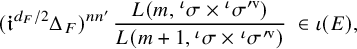$$ \begin{align*}({\mathfrak{i}}^{d_F/2} \Delta_F)^{nn'} \, \frac{L(m, {}^\iota\sigma \times {}^\iota\sigma^{\prime \mathrm{v}})}{L(m+1, {}^\iota\sigma \times {}^\iota\sigma^{\prime \mathrm{v}})} \ \in \iota(E), \end{align*} $$

and furthermore, for every $\gamma \in \mathrm {{Gal}}(\bar {\mathbb {Q}}/\mathbb {Q})$ , we have the reciprocity law:

$$ \begin{align*}\gamma \left( ({\mathfrak{i}}^{d_F/2} \Delta_F)^{nn'} \, \frac{L(m, {}^\iota\sigma \times {}^\iota\sigma^{\prime \mathrm{v}})}{L(m+1, {}^\iota\sigma \times {}^\iota\sigma^{\prime \mathrm{v}})} \right) \ = \ ({\mathfrak{i}}^{d_F/2} \Delta_F)^{nn'} \, \frac{L(m, {}^{\gamma\circ\iota}\sigma \times {}^{\gamma\circ\iota}\sigma^{\prime \mathrm{v}})}{L(m+1, {}^{\gamma\circ\iota}\sigma \times {}^{\gamma\circ\iota}\sigma^{\prime \mathrm{v}})}. \end{align*} $$

5.4.2 Theorem 5.16 implies Conjecture 5.25

If F is in the TR-case, then existence of a critical point implies $nn'$ is even (Corollary 3.14), hence $({\mathfrak {i}}^{d_F/2} \Delta _F)^{nn'} = {\mathfrak {i}}^{d_Fnn'/2} = \pm 1$ that may be absorbed into $\iota (E)$ and ignored from the Galois-equivarance, which is exactly the content of (3) of Theorem 5.16. Assume henceforth that F is in the CM-case. The required compatibility follows from the equality of signatures in the following:

Proposition 5.26.

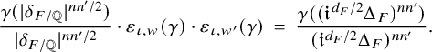$$ \begin{align*}\frac{ \gamma(|\delta_{F/\mathbb{Q}}|^{n n'/2})} {|\delta_{F/\mathbb{Q}}|^{n n'/2}} \cdot \varepsilon_{\iota, w}(\gamma) \cdot \varepsilon_{\iota, w'}(\gamma) \ = \ \frac{ \gamma(({\mathfrak{i}}^{d_F/2} \Delta_F)^{nn'})}{({\mathfrak{i}}^{d_F/2} \Delta_F)^{nn'}}. \end{align*} $$

The proof uses the following lemma.

Lemma 5.27. Let F be a totally imaginary field in the CM-case and suppose $F_1$ the maximal CM subfield of F. Then, as elements of $\mathbb {C}^{\times }/\mathbb {Q}^{\times }$ , we have

$$ \begin{align*}|\delta_{F/\mathbb{Q}}|^{1/2} \ = \ {\mathfrak{i}}^{d_F/2} \cdot \Delta_F \cdot \left(N_{F_1/\mathbb{Q}}(\delta_{F/F_1})\right)^{1/2}. \end{align*} $$

Proof of Lemma 5.27.

Transitivity of discriminant for the tower of fields $F/F_0/\mathbb {Q}$ gives $\delta _{F/\mathbb {Q}} = \delta _{F_0/\mathbb {Q}}^{[F:F_0]} \cdot N_{F_0/\mathbb {Q}}(\delta _{F/F_0}).$ Since the degree $[F:F_0] = 2[F:F_1]$ is even, one has

$$ \begin{align*}|\delta_{F/\mathbb{Q}}|^{1/2} \ = \ |N_{F_0/\mathbb{Q}}(\delta_{F/F_0})|^{1/2} \quad\pmod{\mathbb{Q}^{\times}}. \end{align*} $$

Next, one has $\delta _{F/F_0} = \delta _{F_1/F_0}^{[F:F_1]} \cdot N_{F_1/F_0}(\delta _{F/F_1}),$ by using transitivity of discriminant for the tower of fields $F/F_1/F_0$ ; using the $F_0$ -basis $\{1, \sqrt {D}\}$ for $F_1$ , one has $\delta _{F_1/F_0} = 4D;$ therefore,

$$ \begin{align*} N_{F_0/\mathbb{Q}}(\delta_{F/F_0}) \ = \ N_{F_0/\mathbb{Q}}(4D)^{[F:F_1]} \cdot N_{F_0/\mathbb{Q}} &(N_{F_1/F_0}(\delta_{F/F_1})) \\ &\qquad\quad = \ N_{F_0/\mathbb{Q}}(D)^{[F:F_1]} \cdot N_{F_1/\mathbb{Q}}(\delta_{F/F_1}) \quad\pmod{\mathbb{Q}^{\times}{}^2}. \end{align*} $$

Since $F_1/\mathbb {Q}$ is a CM-extension, $N_{F_1/\mathbb {Q}}(\delta _{F/F_1})> 0$ ; hence,

$$ \begin{align*}|\delta_{F/\mathbb{Q}}|^{1/2} \ = \ |N_{F_0/\mathbb{Q}}(\delta_{F/F_0})|^{1/2} \ = \ |N_{F_0/\mathbb{Q}}(D)|^{[F:F_1]/2} \cdot \left(N_{F_1/\mathbb{Q}}(\delta_{F/F_1})\right)^{1/2} \quad\pmod{\mathbb{Q}^{\times}}. \end{align*} $$

Since $D \ll 0$ in $F_0$ , we see that $(-1)^{[F_0:\mathbb {Q}]}N_{F_0/\mathbb {Q}}(D)> 0$ . Hence,

$$ \begin{align*} |N_{F_0/\mathbb{Q}}(D)|^{[F:F_1]/2} \ = \ ((-1)^{[F_0:\mathbb{Q}]}N_{F_0/\mathbb{Q}}(D))^{[F:F_1]/2} \ &= \ ({\mathfrak{i}}^{[F_0:\mathbb{Q}]} \Delta_{F_1})^{[F:F_1]} \\ &\qquad\qquad\quad = \ {\mathfrak{i}}^{[F_0:\mathbb{Q}][F:F_1]} \Delta_F \ = \ {\mathfrak{i}}^{d_F/2} \Delta_F. \end{align*} $$

After the above lemma, the proof of Proposition 5.26 follows from the following:

Lemma 5.28.

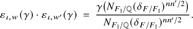$$ \begin{align*}\varepsilon_{\iota, w}(\gamma) \cdot \varepsilon_{\iota, w'}(\gamma) \ = \ \frac{\gamma \left(N_{F_1/\mathbb{Q}}(\delta_{F/F_1})^{nn'/2}\right)}{N_{F_1/\mathbb{Q}}(\delta_{F/F_1})^{nn'/2}}. \end{align*} $$

Proof. Suppose F is a CM field. Then $F = F_1$ ; hence, the right-hand side is $1$ . We contend that in this case, the left-hand side is also $1$ , or that $\varepsilon _{\iota , w}(\gamma ) = \varepsilon _{\iota , w'}(\gamma ).$ One may suppose that the ordering on $\mathrm {{Hom}}(F,E)$ is fixed such that conjugate embeddings are paired: $\mathrm {{Hom}}(F,E) \ = \ \{\tau _1, \bar \tau _1, \tau _2, \bar \tau _2, \dots , \tau _r, \bar \tau _r\}.$ After composing with $\iota : E \to \mathbb {C}$ , one gets an enumeration: $\mathrm {{Hom}}(F,\mathbb {C}) \ = \ \{\eta _1, \bar {\eta }_1, \eta _2, \bar {\eta }_2, \dots , \eta _r, \bar {\eta }_r\}.$ For brevity and, hopefully, additional clarity, denote $e_{\Phi _{w^{\eta , \bar {\eta }}}}^{*} := e_{\Phi _{w^{\eta }}}^{*} \wedge \ e_{\Phi _{w^{\bar {\eta }}}}^{*}$ , and rewrite (2.26) as

(5.29) $$ \begin{align} e_{\Phi_{^\iota \! w}}^{*} \ := \ e_{\Phi_{w^{\eta_1, \bar{\eta}_1}}}^{*} \wedge \cdots \wedge e_{\Phi_{w^{\eta_r, \bar{\eta}_r}}}^{*}. \end{align} $$

The action of $\gamma $ gives

(5.30) $$ \begin{align} (1\otimes \gamma)(e_{\Phi_{^\iota \! w}}^{*}) \ := \ e_{\Phi_{w^{\gamma\circ\eta_1, \gamma\circ\bar{\eta}_1}}}^{*} \wedge \cdots \wedge e_{\Phi_{w^{\gamma\circ\eta_1, \gamma\circ\bar{\eta}_1}}}^{*}. \end{align} $$

The right-hand sides of (5.29) and (5.30) differ by the signature $\varepsilon _{\iota , w}(\gamma )$ that one seeks to identify. Each pair of conjugates embeddings $\{\eta _j, \bar {\eta }_j\}$ corresponds to a place $v_j$ of F; as before, $\eta _j$ is called the distinguished embedding – a base point in that pair of conjugate embeddings. The ordering on $\mathrm {{Hom}}(F,\mathbb {C})$ fixes an ordering $\{v_1,\dots ,v_r\}$ on $\mathrm {S}_\infty (F)$ . Let $\pi _F(\gamma )$ denote the permutation of $\gamma $ on $\mathrm {S}_\infty (F)$ , and $\varepsilon _F(\gamma )$ its signature. For each $1 \leq j \leq r$ , let $l_j = l(w^{\eta _j})$ and $l_j^{*} = l(w^{\bar {\eta }_j})$ ; then $l_j + l_j^{*} = nn'$ since w is balanced. The total degree of $e_{\Phi _{w^{\eta , \bar {\eta }}}}^{*}$ is $nn'$ ; interchanging two successive factors of (5.29) introduces the signature $(-1)^{(nn')^2} = (-1)^{nn'}.$ Finally, let $J_\gamma := \{ j \, | \, \gamma \circ \eta _j \mbox { is not distinguished.}\}.$ Then one has

(5.31) $$ \begin{align} \varepsilon_{\iota, w}(\gamma) \ = \ \varepsilon_F(\gamma)^{nn'} \prod_{j \in J_\gamma} (-1)^{l_jl_j^{*}}; \end{align} $$

since the term $\varepsilon _F(\gamma )^{nn'}$ arises by the permutation of the factors of (5.29) to get the factors of (5.30); and then within each such factor indexed by $j \in J_\gamma $ , the constituent factors in $e_{\Phi _{w^{\eta _j}}}^{*} \wedge \ e_{\Phi _{w^{\bar {\eta }_j}}}^{*}$ get interchanged. Similarly,

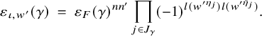(5.32) $$ \begin{align} \varepsilon_{\iota, w'}(\gamma) \ = \ \varepsilon_F(\gamma)^{nn'} \prod_{j \in J_\gamma} (-1)^{l(w^{\prime \eta_j})l(w^{\prime \bar{\eta}_j})}. \end{align} $$

From Lemma 5.1, it follows that $l(w^{\prime \eta _j}) = nn' - l(w^{\eta _j}) = l_j^{*}$ and $l(w^{\prime \bar {\eta }_j}) = nn' - l(w^{\bar {\eta }_j}) = l_j$ ; hence, $(-1)^{l(w^{\prime \eta _j})l(w^{\prime \bar {\eta }_j})} = (-1)^{l_jl_j^{*}}$ ; whence, $\varepsilon _{\iota , w}(\gamma ) = \varepsilon _{\iota , w'}(\gamma ).$

Now suppose F is a totally imaginary field in the CM-case and $F_1$ its maximal CM subfield. In preparation, fix orderings on $\Sigma _F$ , $\Sigma _{F_1}$ and $\mathrm {S}_\infty (F_1)$ in a compatible way as follows:

1. 1. fix an ordering $\{w_1,\dots , w_{r_1}\}$ on $\mathrm {S}_\infty (F_1)$ ;

2. 2. then fix the ordering $\{\nu _1, \nu _2, \dots , \nu _{r_1}, \bar \nu _1, \bar \nu _2, \dots , \bar \nu _{r_1}\}$ , where the pair of conjugate embeddings $\{\nu _j, \bar \nu _j\}$ map to $w_j$ , and recall that we call $\nu _j$ as the distinguished embedding;

3. 3. finally, to fix an ordering on $\Sigma _F$ , let $\Sigma _F(\nu )$ denote the fiber over $\nu \in \Sigma _{F_1}$ under the canonical restriction map $\Sigma _F \to \Sigma _{F_1}$ ; if $\nu < \nu '$ in $\Sigma _{F_1}$ . Then each element in $\Sigma _F(\nu )$ is less than every element of $\Sigma _F(\nu ')$ , and within each fiber $\Sigma _F(\nu )$ , fix any ordering.

The Galois element $\gamma $ induces permutations on $\Sigma _F$ , $\Sigma _{F_1}$ and $\mathrm {S}_\infty (F_1)$ giving the commutative diagram:

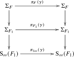
Define $\hat {\pi }_{F}(\gamma )$ to be the permutation of $\Sigma _{F}$ that induces $\pi _{F_1}(\gamma )$ on $\Sigma _{F_1}$ , and

$$ \begin{align*}\mbox{if} \ \pi_{F_1}(\gamma)(\eta) = \eta', \ \mbox{then} \ \hat{\pi}_{F}(\gamma) \mbox{ is an order preserving bijection } \Sigma_F(\nu) \to \Sigma_F(\nu'). \end{align*} $$

Define the permutation $\pi _F'(\gamma )$ of $\Sigma _{F}$ by

(5.33) $$ \begin{align} \pi_F(\gamma) \ = \ \pi_F'(\gamma) \circ \hat{\pi}_{F}(\gamma). \end{align} $$

Observe that $\pi _F'(\gamma )$ induces the identity permutation on $\Sigma _{F_1}$ , and denote $\pi _{\Sigma _F(\nu )}'(\gamma )$ for the permutation that $\pi _F'(\gamma )$ induces on the fiber $\Sigma _F(\nu )$ above $\nu .$ Let $\varepsilon (*)$ denote the signature of a permutation $*$ . The proof of Lemma 5.28 follows from the following two sub-lemmas.

Sublemma 5.34.

$$ \begin{align*}\varepsilon_{\iota, w}(\gamma) \cdot \varepsilon_{\iota, w'}(\gamma) \ = \ \varepsilon(\pi_F'(\gamma))^{nn'} \end{align*} $$

Sublemma 5.35.

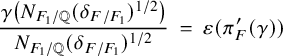$$ \begin{align*}\frac{\gamma \left(N_{F_1/\mathbb{Q}}(\delta_{F/F_1})^{1/2}\right)}{N_{F_1/\mathbb{Q}}(\delta_{F/F_1})^{1/2}} \ = \ \varepsilon(\pi_F'(\gamma)) \end{align*} $$

Proof of Sublemma 5.34.

Define $J_\gamma = \{j \ : \ \pi _{F}(\gamma )(\eta _j) \mbox { is not distinguished}\}$ . Keeping in mind that strongly-pure weights such as $\mu $ and $\mu '$ are the base-change of (strongly-)pure weights from $F_1$ , we deduce that the constituents $({}^\iota \!w^\eta )_{\eta : F \to \mathbb {C}}$ of the Kostant representative ${}^\iota \!w$ are such that if $\eta |_{F_1} = \eta '|_{F_1},$ then ${}^\iota \!w^\eta $ and ${}^\iota \!w^{\eta '}$ are the same element in $\mathfrak {S}_N$ – the Weyl group of $\mathrm {{GL}}_N.$ For $1 \leq j \leq r_1$ , denote $l_j = l({}^\iota \!w^{\eta _{ji}})$ and $l_j^{*} = l({}^\iota \!w^{\bar {\eta }_{ji}}).$ One has $l_j + l_j^{*} = nn'$ since w is balanced. Also, denote $l_\nu = l({}^\iota \!w^{\eta })$ for any $\eta \in \Sigma _F(\nu )$ . We claim that

(5.36) $$ \begin{align} \varepsilon_{\iota, w}(\gamma) \ = \ \varepsilon(\pi_{1\infty}(\gamma))^{(nn'k)^2} \cdot \prod_{j \in J_\gamma} (-1)^{l_jl_j^{*}k^2} \cdot \prod_{\nu \in \Sigma_{F_1}} \varepsilon(\pi^{\prime}_{\Sigma_F(\nu)}(\gamma))^{l_\nu^2}. \end{align} $$

Recall that the signature $\varepsilon _{\iota , w}(\gamma )$ is determined by the action of $\gamma $ on the wedge-product in (2.26): $e_{\Phi _{^\iota \! w}}^{*} = e_{\Phi _{w^{\eta _1}}}^{*} \wedge \cdots \wedge e_{\Phi _{w^{\eta _{d_F}}}}^{*}.$ The proof of (5.36) boils down to becoming aware how the factors in this wedge-product are permuted, and what signature is introduced in un-permuting them. The following scheme depicts from bottom to top, the places of $F_1$ , embeddings of $F_1$ , embeddings of F, and the lengths of the Kostant representatives they parametrize:

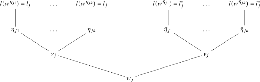
Group together the wedge-factors as follows:

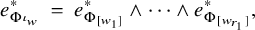$$ \begin{align*}e_{\Phi_{^\iota \! w}}^{*} \ = \ e_{\Phi_{[w_1]}}^{*} \wedge \cdots \wedge e_{\Phi_{[w_{r_1}]}}^{*}, \end{align*} $$

where, for each $1 \leq j \leq r_1$ ,

$$ \begin{align*}e_{\Phi_{[w_j]}}^{*} \ = \ e_{\Phi_{[\nu_j]}}^{*} \wedge e_{\Phi_{[\bar\nu_j]}}^{*}, \end{align*} $$

and for each $\nu _j \in \Sigma _{F_1}$ ,

$$ \begin{align*}e_{\Phi_{[\nu_j]}}^{*} = e_{\Phi_{w^{\eta_{j1}}}}^{*} \wedge \dots \wedge e_{\Phi_{w^{\eta_{jk}}}}^{*}, \quad e_{\Phi_{[\bar\nu_j]}}^{*} = e_{\Phi_{w^{\bar{\eta}_{j1}}}}^{*} \wedge \dots \wedge e_{\Phi_{w^{\bar{\eta}_{jk}}}}^{*}. \end{align*} $$

Recall that $e_{\Phi _{w^{\eta _{ji}}}}^{*}$ has degree $l_j$ and $e_{\Phi _{w^{\bar {\eta }_{ji}}}}^{*}$ has degree $l_j^{*}.$ Hence, $e_{\Phi _{[\nu _j]}}^{*}$ has degree $kl_j$ , and $e_{\Phi _{[\bar \nu _j]}}^{*}$ has degree $kl_j^{*}.$ Therefore, $e_{\Phi _{[w_j]}}^{*}$ has degree $kl_j + kl_j^{*} = knn'$ . Now, the permutation $\pi _{1\infty }(\gamma )$ on $S_\infty (F_1) = \{w_1,\dots ,w_{r_1}\}$ can be undone by the signature $\varepsilon (\pi _{1\infty }(\gamma ))^{(nn'k)^2}.$ Next, only for those $j \in J_\gamma $ , the two factors in $e_{\Phi _{[\nu _j]}}^{*} \wedge e_{\Phi _{[\bar \nu _j]}}^{*}$ get interchanged, giving the signature $(-1)^{l_jl_j^{*}k^2}$ . Finally, adjusting for the action of $\gamma $ on $\Sigma _{F_1}$ (i.e., now working with $\pi ^{\prime }_F(\gamma )$ , which only permutes internally within each fiber $\Sigma _F(\nu )$ over $\nu \in \Sigma _{F_1}$ ), one sees the signature $\varepsilon (\pi ^{\prime }_{\Sigma _F(\nu )}(\gamma ))^{l_\nu ^2}$ for each such $\nu .$ This proves the claim (5.36).

For any integer a, since $a^2 \equiv a \ \pmod {2}$ , (5.36) simplifies to

(5.37) $$ \begin{align} \varepsilon_{\iota, w}(\gamma) \ = \ \varepsilon(\pi_{1\infty}(\gamma))^{nn'k} \cdot \prod_{j \in J_\gamma} (-1)^{l_jl_j^{*}k} \cdot \prod_{\nu \in \Sigma_{F_1}} \varepsilon(\pi^{\prime}_{\Sigma_F(\nu)}(\gamma))^{l_\nu}. \end{align} $$

Similarly, using the relation of $w'$ with w, one has

(5.38) $$ \begin{align} \varepsilon_{\iota, w'}(\gamma) \ = \ \varepsilon(\pi_{1\infty}(\gamma))^{nn'k} \cdot \prod_{j \in J_\gamma} (-1)^{l_j^{*}l_jk^2} \cdot \prod_{\nu \in \Sigma_{F_1}} \varepsilon(\pi^{\prime}_{\Sigma_F(\nu)}(\gamma))^{l_\nu^{*}}. \end{align} $$

Multiply (5.37) and (5.38) to get

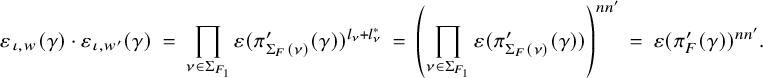$$ \begin{align*}\varepsilon_{\iota, w}(\gamma) \cdot \varepsilon_{\iota, w'}(\gamma) \ = \ \prod_{\nu \in \Sigma_{F_1}} \varepsilon(\pi^{\prime}_{\Sigma_F(\nu)}(\gamma))^{l_\nu + l_\nu^{*}} \ = \ \left(\prod_{\nu \in \Sigma_{F_1}} \varepsilon(\pi^{\prime}_{\Sigma_F(\nu)}(\gamma))\right)^{nn'} \ = \ \varepsilon(\pi_{F}'(\gamma))^{nn'}.\\[-48pt] \end{align*} $$

Proof of Sublemma 5.35.

For $x \in F_1^{\times }$ , one has $N_{F_1/\mathbb {Q}}(x) = \prod _{\nu \in \Sigma _{F_1}}\nu (x)> 0.$ Let $\{\rho _1,\dots ,\rho _k\}$ denote the set of all embeddings of F into $\bar {F_1}$ over $F_1$ , for some algebraic closure $\bar {F_1}$ of $F_1$ ; let $\{\omega _1,\dots ,\omega _k\}$ be an $F_1$ -basis for F; then $\delta _{F/F_1} = \det [\rho _i(\omega _j)]^2.$ Hence,

$$ \begin{align*}N_{F_1/\mathbb{Q}}(\delta_{F/F_1}) \ = \ \prod_{\nu \in \Sigma_{F_1}} \nu(\det[\rho_i(\omega_j)]^2) \ = \ \prod_{\nu \in \Sigma_{F_1}} \det[\rho_i^\nu(\omega_j)]^2, \end{align*} $$

where $\{\rho _1^\nu , \dots , \rho _k^\nu \}$ is the set of all embeddings of F into $\mathbb {C}$ that restrict to $\nu : F_1 \to \mathbb {C}.$ We may take $\rho _i^\nu $ to be $\tilde \nu \circ \rho _i$ for any extension $\tilde \nu : \bar {F_1} \to \mathbb {C}$ of $\nu .$ Whence,

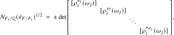(5.39) $$ \begin{align} N_{F_1/\mathbb{Q}}(\delta_{F/F_1})^{1/2} \ = \ \pm \det \left[\begin{array}{cccc} [\rho_i^{\nu_1}(\omega_j)] & & & \\ & [\rho_i^{\nu_2}(\omega_j)] & & \\ & & \ddots & \\ & & & [\rho_i^{\nu_{d_1}}(\omega_j)] \end{array}\right], \end{align} $$

where the appropriate sign $\pm $ is chosen to make the right-hand side positive. Each block $[\rho _i^{\nu }(\omega _j)]$ is a $k \times k$ -block. Apply $\gamma $ to (5.39), and the change in the sign of the determinant on the right is the requisite sign $\gamma \left (N_{F_1/\mathbb {Q}}(\delta _{F/F_1})^{1/2}\right )/N_{F_1/\mathbb {Q}}(\delta _{F/F_1})^{1/2}.$ The blocks are permuted according to $\pi _{F_1}(\gamma )$ which does not change the sign. Hence, the signature is accounted for by assuming that the blocks remain where they are and looking at how each block’s rows are permuted internally; in other words, keeping (5.33) in mind, the requisite signature is

$$ \begin{align*}\prod_{\nu \in \Sigma_{F_1}} \varepsilon(\pi^{\prime}_{\Sigma_F(\nu)}(\gamma)) \ = \ \varepsilon(\pi_{F}^{\prime}(\gamma)).\\[-48pt] \end{align*} $$

This concludes the proof of Lemma 5.28.

This concludes the proof of Proposition 5.26, proving compatibility of our main theorem with Deligne’s conjecture.

5.5 An example

If we take $n = n' = 1$ , then the main result and techniques are all due to Harder [22]. However, the signature $\varepsilon _{\iota , w}(\gamma ) \cdot \varepsilon _{\iota , w'}(\gamma ),$ that can be nontrivial in general, is missing in [22]. Furthermore, the subtle distinction between when F is in the CM-case and when it is in the TR-case is not seen in [22] and it becomes apparent only in the larger context of this article. This case $n = n' = 1$ is also extensively discussed in [42], wherein examples are constructed to show the nontriviality of these signatures. As an alternative, it is worth the effort to illustrate the content of the main theorem in the simplest nontrivial example: when $n = n' = 1$ and F is an imaginary quadratic field, not so much by appealing to Harder [22], or this article, but rather via recourse to modular forms of CM type. Here, $\sigma $ and $\sigma '$ are both algebraic Hecke characters, and the main theorem concerns the ratios of successive critical values of the L-function attached to the algebraic Hecke character: $\chi = \sigma \sigma ^{\prime -1}.$ After relabelling, take $\sigma = \chi $ an algebraic Hecke character, and for $\sigma '$ , take the trivial character. This $\mathrm {{GL}}(1)$ -example is instructive, and was helpful to the author to see some finer details.

For an imaginary quadratic field $F,$ let $\mathrm {{Hom}}(F,\mathbb {C}) = \{\eta , \bar {\eta }\}$ ; the choice of $\eta $ is not canonical; it induces an isomorphism $\eta : F_\infty \simeq \mathbb {C}.$ Let $\chi : F^{\times } \backslash \mathbb {A}_F^{\times } \to \mathbb {C}^{\times }$ be an algebraic Hecke character; this means that $\chi $ is a continuous homomorphism whose infinite component $\chi _\infty : F_\infty ^{\times } \to \mathbb {C}^{\times }$ is of the form $\chi _\infty (z) = z^p \bar {z}^q,$ for integers p and q. Then $\chi \in \mathrm {{Coh}}(\mathrm {{GL}}_1/F, \mu )$ with $\mu = (\mu ^\eta , \mu ^{\bar {\eta }})$ and $\mu ^\eta = -p$ and $\mu ^{\bar {\eta }} = -q.$ The weight $\mu $ is strongly-pure with purity weight $\mathbf {{w}} = -p-q.$ One also has

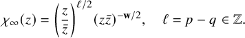$$ \begin{align*}\chi_\infty(z) = \left(\frac{z}{\bar{z}}\right)^{\ell/2} (z\bar{z})^{-\mathbf{{w}}/2}, \quad \ell = p-q \in \mathbb{Z}. \end{align*} $$

As recalled in (3.3), the $\Gamma $ -factors at infinity (up to nonzero constants and exponentials) on either side of the functional equation are

$$ \begin{align*}L_\infty(s, \chi) \sim \Gamma(s - \tfrac{\mathbf{{w}}}{2} + \tfrac{|\ell|}{2}), \quad L_\infty(1-s, \chi^{-1}) \sim \Gamma(1-s + \tfrac{\mathbf{{w}}}{2} + \tfrac{|\ell|}{2}). \end{align*} $$

Assume, without any loss of generality (if necessary, replacing $\chi $ by $\chi ^{-1}$ ), that $\ell \geq 0,$ (i.e., $p \geq q).$ Then $L_\infty (s, \chi ) \sim \Gamma (s+p)$ and $L_\infty (1-s, \chi ^{-1}) \sim \Gamma (1-s-q).$ The critical set for $L(s, \chi )$ is the set of $\ell $ consecutive integers: $\{1-p, \, 2-p, \dots , \, -q\}.$ The critical set is nonempty if $\ell \geq 1$ , and we have $\ell $ many critical points and $\ell -1$ pairs of successive critical points. The cuspidal width $\ell (\mu , 0)$ between $\mu $ and the weight $\mu ' = 0$ is $\ell (\mu , 0) = \ell .$ If we were to apply the main theorem to the pair $\chi $ and the trivial Hecke character (which is cohomological with respect to $\mu '=0$ ), then the combinatorial lemma (Lemma 3.16) imposes the condition $\ell \geq 2,$ and Theorem 5.16 gives a rationality result for the ratios $L(m,\chi )/L(m+1,\chi )$ of all successive critical values. This theorem can also be seen independently by appealing to the rationality results of Shimura for L-functions of modular forms.

Take $\pi = \pi (\chi ) = \text {AI}_F^{\mathbb {Q}}(\chi )$ to be the automorphic induction of $\chi $ from F to $\mathbb {Q}$ . Then $\pi $ is a cuspidal automorphic representation of $\mathrm {{GL}}_2(\mathbb {A}_{\mathbb {Q}}).$ The representation $\pi _\infty $ at the infinite place is, by definition, $\text {AI}_{\mathbb {C}}^{\mathbb {R}}(\chi _\infty ),$ which in turn is defined by asking for its Langlands parameter to be the induced representation $\mathrm {{Ind}}_{W_{\mathbb {C}}}^{W_{\mathbb {R}}}(\chi _\infty ) = \mathrm {{Ind}}_{\mathbb {C}^{\times }}^{W_{\mathbb {R}}}(z \mapsto \left (\frac {z}{\bar {z}}\right )^{\ell /2}) \otimes |\ |_{\mathbb {R}}^{-\mathbf {{w}}/2}.$ This is exactly the representation that has cohomology with respect to the irreducible representation of $\mathrm {{GL}}(2)$ with highest weight $\lambda = (p,q).$ By the standard dictionary between modular forms and automorphic representations (see, for example, Gelbart [13]), there is a primitive modular form $f_\chi $ of weight $k = p-q+1$ such that $\pi (\chi ) = \pi (f_\chi ) \otimes |\ |^{-\mathbf {{w}}/2}.$ One of the properties of this dictionary gives us the following equality of L-functions:

$$ \begin{align*}L(s, f_\chi) \ = \ L(s - \tfrac{(k-1)}{2}, \pi(f_\chi)) \ = \ L(s - \tfrac{(k-1)}{2} + \tfrac{\mathbf{{w}}}{2}, \pi(\chi)) \ = \ L(s-p, \chi). \end{align*} $$

The critical set for $L(s, f_\chi )$ is the string of integers $\{1,2,\dots ,k-1\}.$ A word about the normalizations of these L-functions: first of all, $L(s, f_\chi )$ is the Hecke L-function of the modular form $f_\chi $ , which has a functional equation with respect to $s \leftrightarrow k-s$ . For a cuspidal automorphic representation $\pi $ , as applied to $\pi (\chi )$ or to $\pi (f_\chi )$ , the functional equation is with respect to $s \leftrightarrow 1-s$ . The L-function $L(s,\chi )$ also has a functional equation with respect to $s \leftrightarrow 1-s$ . Furthermore, for any Dirichlet character $\omega $ , by which we mean a character $\omega : \mathbb {Q}^{\times } \backslash \mathbb {A}_{\mathbb {Q}}^{\times } \to \mathbb {C}^{\times }$ of finite-order, there is the equality

$$ \begin{align*}L(s, f_\chi, \omega) \ = \ L(s-p, \chi \otimes \omega^F), \end{align*} $$

where $\omega ^F := \omega \circ N_{F/\mathbb {Q}}$ is the base-change of $\omega $ from $\mathbb {Q}$ to F. In particular, if $\omega = \omega _{F/\mathbb {Q}}$ is the quadratic Dirichlet character of $\mathbb {Q}$ attached to F by class field theory, then

$$ \begin{align*}L(s, f_\chi, \omega_{F/\mathbb{Q}}) \ = \ L(s, f_\chi), \end{align*} $$

since the base-change of $\omega _{F/\mathbb {Q}}$ back to F is the trivial character. This is also seen at the level of representations since $\pi (\chi ) \simeq \pi (\chi ) \otimes \omega _{F/\mathbb {Q}}.$

From Shimura [49] applied to $f_\chi $ , there exists two periods $u^\pm (f_\chi ) \in \mathbb {C}^{\times }$ , such that for any critical integer $r \in \{1,\dots ,k-1\}$ , and any primitive Dirichlet character $\psi $ , one has

where $\mathfrak {g}(\psi )$ is the Gauß sum of $\psi $ , and the choice of periods is dictated by the parities of r and $\psi $ via $\psi (-1) = \pm (-1)^r$ ; and $\approx $ is a simplified notation to mean that the ratio of the left-hand side divided by everything on the right-hand side is algebraic, and is $\mathrm {{Gal}}(\bar {\mathbb {Q}}/\mathbb {Q})$ -equivariant:

The finite part of the L-function $L_f(r, f_\chi , \psi )$ is completed using the archimedean $\Gamma $ -factor . In terms of the completed L-function, the above relation takes the form

$$ \begin{align*} L(r, f_\chi, \psi) \ \approx \ {\mathfrak{i}}^r u^\pm(f_\chi) \mathfrak{g}(\psi). \end{align*} $$

Take $r=1$ and use the above relation once for $\psi $ the trivial character and then for $\psi = \omega _{F/\mathbb {Q}}$ to deduce

$$ \begin{align*} u^+(f_\chi) \ \approx \ u^-(f_\chi) \, \mathfrak{g}(\omega_{F/\mathbb{Q}}). \end{align*} $$

Next, apply Shimura’s result to $L(s,f_\chi )$ for $s = r$ and $s = r+1$ , where $r \in \{1,\dots ,k-2\}$ (possible when $k \geq 3$ , that is, $\ell \geq 2$ ), and divide one by the other to deduce

$$ \begin{align*}\frac{L(r,f_\chi)}{L(r+1,f_\chi)} \ \approx \ {\mathfrak{i}} \, \mathfrak{g}(\omega_{F/\mathbb{Q}}), \end{align*} $$

while using ${\mathfrak {i}}^2 \in \mathbb {Q}^{\times }$ and $\mathfrak {g}(\omega _{F/\mathbb {Q}})^2 \in \mathbb {Q}^{\times }.$ Since $L(s, f_\chi ) = L(s-p, \chi ),$ and putting $r-p = m,$ one gets for the ratio of two successive critical values of the completed L-function of $\chi $ the rationality result

$$ \begin{align*} {\mathfrak{i}} \, \mathfrak{g}(\omega_{F/\mathbb{Q}}) \frac{L(m, \chi)}{L(m+1,\chi)} \in \bar{\mathbb{Q}}, \end{align*} $$

and furthermore,

$$ \begin{align*} \gamma\left( {\mathfrak{i}} \, \mathfrak{g}(\omega_{F/\mathbb{Q}}) \frac{L(m, \chi)}{L(m+1, \chi)}\right) \ = \ {\mathfrak{i}} \, \mathfrak{g}(\omega_{F/\mathbb{Q}}) \frac{L(m, {}^\gamma\chi)}{L(m+1, {}^\gamma\chi)}, \quad \forall \gamma \in \mathrm{{Gal}}(\bar{\mathbb{Q}}/\mathbb{Q}). \end{align*} $$

One has used that ${}^\gamma f_\chi = f_{{}^\gamma \chi }$ which follows from the definition of $f_\chi $ (see [48, Sect. 5]). To see that the above result is indeed an instance of Theorem 5.16, one needs the basic fact about quadratic Gauss sums: ${\mathfrak {i}} \, \mathfrak {g}(\omega _{F/\mathbb {Q}}) = |\delta _{F/\mathbb {Q}}|^{1/2} \ \pmod {\mathbb {Q}^{\times }}$ . It is shown in [41] that this example generalizes from $\mathrm {{GL}}(1)$ over an imaginary quadratic extension to $\mathrm {{GL}}(n)$ over a CM field.