A rasterization-based ray-tracing method for laser–plasma interactions

Abstract

This paper introduces a novel ray-tracing methodology for various gradient-index materials, particularly plasmas. The proposed approach utilizes adaptive-step Runge–Kutta integration to compute ray trajectories while incorporating an innovative rasterization step for ray energy deposition. By removing the requirement for rays to terminate at cell interfaces – a limitation inherent in earlier cell-confined approaches – the numerical formulation of ray motion becomes independent of specific domain geometries. This facilitates a unified and concise tracing method compatible with all commonly used curvilinear coordinate systems in laser–plasma simulations, which were previously unsupported or prohibitively complex under cell-confined frameworks. Numerical experiments demonstrate the algorithm’s stability and versatility in capturing diverse ray physics across reduced-dimensional planar, cylindrical and spherical coordinate systems. We anticipate that the rasterization-based approach will pave the way for the development of a generalized ray-tracing toolkit applicable to a broad range of fluid simulations and synthetic optical diagnostics.

1 Introduction

The interaction between high-power lasers and plasmas plays a crucial role in inertial confinement fusion (ICF), laser wakefield acceleration and advanced diagnostic techniques. Tracing rays in laser-generated plasmas^{[ 1 ]} is the primary focus of this paper. Plasma as a medium is characterized by its spatially varying refractive index, which belongs to a family termed gradient-index materials. Geometric optics are often used for gradient-index ray tracing. Although the theoretical foundations of geometric optics were established nearly two centuries ago through Hamiltonian optics^{[ 2 , 3 ]}, good-quality applications have only become feasible with the advent of modern computational power and algorithmic advancements, which enable us to synthesize images of black holes^{[ 4 ]}, study the architecture of biological eyes^{[ 5 ]}, design advanced antennas^{[ 6 ]} and lenses^{[ 7 , 8 ]} and optimize laser energy deposition in fusion plasmas^{[ 9 – 11 ]}. Beyond the inherently dynamic and inhomogeneous nature of flow fields, plasmas exhibit unique ray–medium interactions. Light induces electron oscillations and heats the plasma through collisions^{[ 12 ]}; nonuniformities in the beam energy distribution give rise to various instabilities^{[ 13 – 15 ]}; and frequency differences between beams can even facilitate energy transfer from one beam to another^{[ 16 , 17 ]}. Ray-tracing algorithms designed to capture these phenomena must balance physical fidelity with computational efficiency.

When it comes to numerical implementation, if the medium’s refractive index exhibits certain symmetry and trajectories are the sole quantities of interest, as in most lens designs, tracing packages employing Runge–Kutta (RK)^{[ 18 ]} or advanced symplectic-RK methods^{[ 19 ]} have demonstrated remarkable efficiency. In such cases, rays do not reciprocally alter medium properties. For plasmas, however, the spatial distribution of electron density determines the trajectory of incident laser rays. In turn, the energy loss of the laser becomes the critical physical quantity that corresponds to the thermal gain of the fluid. The challenge here lies in the fact that energy deposition and ray trajectories are defined on two distinct grid systems: deposition is a field quantity that follows the structured fluid cells, while ray trajectories are defined by a sequence of discrete nodes, with varying positions and numbers. Consequently, a tracing algorithm must determine which fluid cells should receive the energy loss associated with each small segment of the ray. In practice, selecting an appropriate tracing logic to ensure compatibility between the fluid grid and ray trajectory coordinate systems is the starting point for plasma ray tracing. In previous treatments, the most commonly used is the ‘cell-confined’ logic: a ray begins at the entry point on the cell face, propagates within the cell along a predefined path and exits at another point on the cell face. The term ‘confined’ emphasizes that ray nodes are precisely the intersection points of the ray with the cell faces. Rays are traced on a cell-by-cell basis and, at each step, the energy loss of the ray is deposited into the cell it currently traverses.

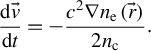
Many commonly used radiation-hydrodynamics (RHD) codes adopt cell-confined logic in their laser modules. MULTI-2D^{[ 20 ]} assumes straight-line ray paths within each cell, ignoring refraction; FLASH^{[ 21 , 22 ]} and RHDLPP^{[ 23 ]} incorporate curved trajectories to account for refraction; while proprietary codes such as xRAGE^{[ 24 ]} and DRACO^{[ 25 ]} use the Mazinisin tracing module^{[ 26 ]}, which supports curved trajectories and energy transfer between rays. FLASH, RHDLPP and Mazinisin tracing can all be traced back to the ‘cell-AVG’ algorithm proposed by Kaiser^{[ 27 ]}. Building on cell-confined methods, cell-AVG further assumes a linear variation of electron density within each cell. In coordinate systems with globally parallel cell faces (e.g., Cartesian grids), cell-AVG ray trajectories can be analytically expressed as quadratic functions. As a result, the ray entry and exit points on cell faces (as shown in Figure 1(a)) can be efficiently determined with minimal computational cost.

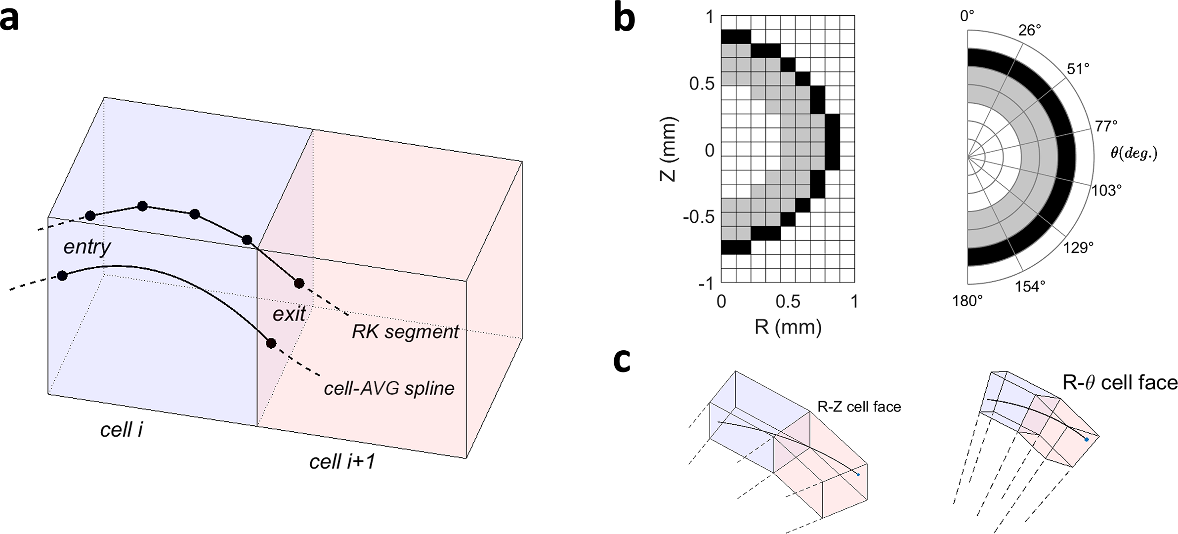
Figure 1 (a) Ray trajectories through cells: one follows the cell-AVG curved path, and the other represents the cell-confined RK straight-line path. (b) A spherical target represented in 2D $R-Z$ cylindrical coordinates and $R-\theta$ spherical coordinates. (c) Truncated-wedge cells derived from 2D cylindrical or spherical grids, lifted into a temporary 3D space for ray tracing.

Despite its success and widespread adoption, cell-confined tracing faces notable challenges in certain applications, for example, tracing rays in cylindrical and spherical coordinate systems. When plasmas exhibit symmetry, curved coordinate systems are often employed to reduce dimensionality, as illustrated in Figure 1(b) with a two-dimensional (2D) cylindrical or spherical coordinate system for an ICF layered target. In these cases, fluid cell faces are curved, and the size and orientation of cells are not globally uniform. Ray trajectories must therefore be constructed in the local reference frame of the individual fluid cells, and the entry and exit points of rays cannot be expressed analytically. Instead, iterative methods are required to approximate these intersection points (see Ref. [22], Section 18.4.9), which reduces computational performance and introduces significant parallelization overhead. Similarly, in ‘reduced-dimensional’ simulations, where lasers interact with one-dimensional (1D) or 2D fluid domains at oblique angles, the fluid cells must be temporarily extruded into truncated-wedge cells (TW-cells) and stacked up to approximate the three-dimensional (3D) structure, as shown in Figures 1(b) and 1(c), where ray calculations are performed at the entry and exit points on the surfaces of each wedge. The formation of TW-cells requires different tracing codes for every laser–fluid geometry combination, making implementation highly complex and significantly increasing the difficulty of incorporating user-defined ray physics.

It is worth noting that, in addition to the cell-AVG method, the FLASH code provides an alternative RK-based tracing approach called ‘CIRK’ (see Section 18.4.4.3 of Ref. [22]). This method allows ray trajectories to be recorded in a 3D Cartesian coordinate system $[x,y,z]$ , while fluid fields are recorded in a 2D cylindrical coordinate system $\left[r,z\right]$ , with their interactions bridged through Jacobian transformations. This avoids the complexity of describing ray trajectory splines in curvilinear coordinates. However, its adoption is far less widespread than cell-AVG in plasma simulations due to inherent limitations. Firstly, CIRK relies on high-order interpolation of fluid fields to propagate rays, but such interpolated fields are susceptible to oscillations, potentially resulting in incorrect ray refraction. Secondly, CIRK still requires ray nodes to align with cell faces, achieved through iterative adjustments of the RK step size. Consequently, this method does not fundamentally resolve the coordination challenges between ray trajectories and fluid grids.

The limitations of these cell-confined methods have constrained the implementation of curved coordinate systems in mainstream RHD programs. For instance, MULTI-2D does not include refraction modeling in spherical coordinates, and FLASH lacks support for spherical ray tracing entirely. Considering the prevalent use of curved coordinate systems and the substantial computational burden associated with ray tracing in laser–plasma simulations, there remains a pressing need for further innovation in ray-tracing methodologies.

This paper proposes a novel ray-tracing approach based on rasterization, aimed at achieving high-performance plasma ray tracing in curved coordinate systems and reduced-dimensional simulations. The key feature of this method is the decoupling of ray trajectory calculation from energy deposition. In the trajectory-solving phase, ray propagation is performed using adaptive step-size RK–Fehlberg (RKF) integration^{[ 28 ]}, where the step size is determined physically by the gradient of the background medium rather than being constrained to terminate at cell boundaries. This eliminates the need for iterative searches for cell entry and exit points or the construction of TW-cells. In the deposition-solving phase, rasterization techniques are employed to segment the ray’s energy loss based on its intersection with the fluid grid and redistribute it to the corresponding fluid cells, and the energy deposition field is accumulated accordingly.

The key innovation of the rasterization-based method lies in the development of a unified and significantly simplified tracing framework, capable of handling various curved coordinate systems and reduced-dimensional simulations – an achievement unattainable with previous cell-confined approaches. Furthermore, rasterization-based tracing provides a practical advantage: ray trajectories are recorded globally in a Cartesian coordinate system rather than being constrained by the curved coordinates of the fluid. This greatly simplifies the incorporation of additional ray physics, making the process intuitive and user-friendly. Although designed primarily for plasma media, this rasterization-based approach is also applicable to a broader range of gradient-index materials.

The remainder of this paper is organized as follows. Section 2 outlines the physical foundations of ray motion and energy deposition. Section 3 details the complete workflow for constructing a rasterized ray-tracing program. Section 4 presents test cases demonstrating the program’s capabilities in planar, spherical and cylindrical coordinates, including comparisons of ray trajectories, energy deposition and frequency shift physics with analytical results. Finally, Section 5 concludes the paper and discusses future perspectives.

2 Physics of ray motion and deposition in plasma

2.1 Ray motion equation

The ray motion equation can be derived from either the Hamiltonian geometric optics framework^{[ 19 ]} or directly from wave equations. In this paper, we adopt the Helmholtz equation as the starting point. For a monochromatic wave $E\left(\vec{r},t\right)={E}_{\mathrm{a}}\left(\vec{r}\right){e}^{- i\omega t}$ , the electric field amplitude ${E}_{\mathrm{a}}$ satisfies the scalar equation:

(1) $$\begin{align}{\nabla}^2{E}_{\mathrm{a}}\left(\vec{r}\right)+{k}_0^2\varepsilon \left(\omega, \vec{r}\right){E}_{\mathrm{a}}\left(\vec{r}\right)=0,\end{align}$$

where $c$ is the speed of light in vacuum, ${k}_0=\omega /c$ is the vacuum wave number and $\varepsilon \left(\omega, \vec{r}\right)={\varepsilon}^{\prime}\left(\omega, \vec{r}\right)+i{\varepsilon}^{{\prime\prime}}\left(\omega, \vec{r}\right)$ represents the medium’s complex dielectric function. We assume the electric field can be expressed as a combination of a slowly varying envelope and a rapidly oscillating phase ${E}_{\mathrm{a}}\left(\vec{r}\right)=A\left(\vec{r}\right){e}^{ik_0S\left(\vec{r}\right)}$ , where $S\left(\vec{r}\right)$ is referred to as the ‘eikonal’. Substituting this trial solution into Equation (1), the imaginary and real parts respectively yield the following:

(2) $$\begin{align}2\left(\nabla A\right)\cdot \left(\nabla S\right)+A{\nabla}^2S+{k}_0{\varepsilon}^{{\prime\prime} }A=0,\end{align}$$

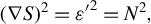(3) $$\begin{align}{\left(\nabla S\right)}^2={\varepsilon^{\prime}}^2={N}^2,\end{align}$$

where $N$ is defined the medium refractive index. Equation (2) is the transport equation, which can be rewritten as $\nabla \cdot \left({A}^2c\nabla S\right)=-{ck}_0{\varepsilon}^{{\prime\prime} }{A}^2$ . If we draw an analogy between the scalar field $S$ and a velocity potential, its gradient $\nabla S$ represents an irrotational steady flow field with a group velocity of $c\nabla S$ . The flowing particles possess an energy density ${A}^2$ , with an absorption rate per unit time given by $-{ck}_0{\varepsilon}^{{\prime\prime} }{A}^2$ . Equation (3), known as the eikonal equation, belongs to the Hamilton–Jacobi family. The eikonal equation allows us to transition to a ‘ray particle’ perspective: let $\vec{r}(s)$ denote the position vector as a function of the arc length $s$ , where $\mathrm{d}{s}^2=\mathrm{d}\vec{r}\cdot \mathrm{d}\vec{r}$ . In this perspective, ray motion is everywhere perpendicular to the surfaces of constant phase, with the motion vector given by $\mathrm{d}\vec{r}/\mathrm{d}s=\nabla S/N$ .

Since solving directly for the eikonal $S$ is often challenging, we take an additional derivative with respect to the arc length:

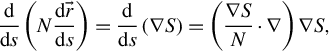$$\begin{align*} \frac{\mathrm{d}}{\mathrm{d}s}\left(N\frac{\mathrm{d}\vec{r}}{\mathrm{d}s}\right)=\frac{\mathrm{d}}{\mathrm{d}s}\left(\nabla S\right)=\left(\frac{\nabla S}{N}\cdot \nabla \right)\nabla S, \end{align*}$$

where the differential along the arc is transformed into a directional derivative along the velocity unit vector. Taking the gradient of the eikonal equation $\nabla {N}^2=\nabla {\left(\nabla S\right)}^2=\nabla \left(\nabla S\cdot \nabla S\right)=2\left(\nabla S\cdot \nabla \right)\nabla S$ , and substituting it into the right-hand side of the equation above, we obtain a ray motion equation that does not explicitly rely on the eikonal equation and is well-suited for numerical discretization:

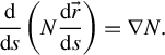(4) $$\begin{align}\frac{\mathrm{d}}{\mathrm{d}s}\left(N\frac{\mathrm{d}\vec{r}}{\mathrm{d}s}\right)=\nabla N.\end{align}$$

2.2 Plasma ray trajectory and energy deposition

The plasma dielectric function is expressed as

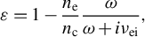(5) $$\begin{align}\varepsilon =1-\frac{n_{\mathrm{e}}}{n_{\mathrm{c}}}\frac{\omega }{\omega +i{\nu}_{\mathrm{ei}}},\end{align}$$

where ${n}_{\mathrm{e}}$ is the electron density, critical density ${n}_{\mathrm{c}}={\omega}^2{m}_{\mathrm{e}}/\left(4\pi {e}^2\right)$ , ${m}_{\mathrm{e}}$ is the electron mass, $e$ is the electron charge and ${\nu}_{\mathrm{ei}}$ is the electron collision frequency (refer to Ref. [1], equation 10.133):

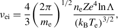(6) $$\begin{align}{\nu}_{\mathrm{ei}}=\frac{4}{3}{\left(\frac{2\pi }{m_{\mathrm{e}}}\right)}^{1/2}\frac{n_{\mathrm{e}}{Ze}^4\mathit{\ln}\Lambda}{{\left({k}_{\mathrm{B}}{T}_{\mathrm{e}}\right)}^{3/2}},\end{align}$$

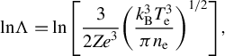(7) $$\begin{align}\mathit{\ln}\Lambda =\mathit{\ln}\left[\frac{3}{2{Ze}^3}{\left(\frac{k_{\mathrm{B}}^3{T}_{\mathrm{e}}^3}{\pi {n}_{\mathrm{e}}}\right)}^{1/2}\right],\end{align}$$

where $Z$ is the effective charge, ${k}_{\mathrm{B}}{T}_{\mathrm{e}}$ represents the electron energy and $\mathit{\ln}\Lambda$ is the Coulomb logarithm. When the electron collision frequency is much smaller than the wave frequency (a condition satisfied in most plasma corona absorption; for complete field reconstruction and proper absorption treatment, see Ref. [29]), the dielectric function simplifies to $\varepsilon \approx 1-{n}_{\mathrm{e}}/{n}_{\mathrm{c}}\left(1-i{\nu}_{\mathrm{ei}}/\omega \right)$ .

To calculate inverse-bremsstrahlung absorption, we define a virtual time $\mathrm{d}t=\mathrm{d}s/\!\!\mid \vec{v}\mid$ where $\vec{v}=c\nabla S= cN\widehat{v}$ is the group velocity of the electromagnetic wave in plasma. Substituting the imaginary part of the dielectric function into the transport equation, and integrating over the trajectory parameter $t$ (rather than $s$ , since absorption depends on the time the wave packet resides in the absorbing medium), we obtain the evolution of the ray energy $P\propto {A}^2$ :

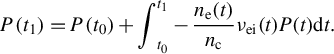(8) $$\begin{align}P\left({t}_1\right)=P\left({t}_0\right)+{\int}_{t_0}^{t_1}-\frac{n_{\mathrm{e}}(t)}{n_{\mathrm{c}}}{\nu}_{\mathrm{ei}}(t)P(t)\mathrm{d}t.\end{align}$$

Using the virtual time $t$ in place of $\mathrm{d}s$ in Equation (4), and incorporating the plasma refractive index, Equation (4) can be reformulated as two first-order ordinary differential equations:

(9) $$\begin{align}\frac{\mathrm{d}\vec{r}}{\mathrm{d}t}=\vec{v}, \qquad\qquad\end{align}$$

(10) $$\begin{align}\frac{\mathrm{d}\vec{v}}{\mathrm{d}t}=-\frac{c^2\nabla {n}_{\mathrm{e}}\left(\vec{r}\right)}{2{n}_{\mathrm{c}}}.\end{align}$$

Given the initial ray position and speed, Equations (9) and (10) delineate a trajectory. A large ensemble of rays collectively models the refraction and reflection of the entire laser beam. In numerical solutions, ray trajectories are represented as a sequence of discrete spatial nodes connected by small line segments, whose shapes are determined by locally interpolated plasma fields and their gradients.

2.3 Rasterization ray-trace concept

Ray trajectory nodes are inherently unstructured in space; forcing them to conform to the structured fluid cells is the primary source of complexity in cell-confined algorithms. This raises an important question: can the constraints imposed by fluid cells on rays be removed?

A similar problem arises in computer graphics, where 3D unstructured models are projected onto structured 2D observation grids. For example, capturing an image of a 3D luminous object with a virtual camera involves determining the model’s vertices, surface emissivity and ray transport trajectories through the medium, followed by a rasterization step (see Ref. [30], Chapter 7, and Ref. [31], Section 15.6) to accumulate signals received by camera pixels. This concept can be directly applied to ray tracing in plasma: the refractive medium and the camera correspond to the fluid domain, while pixel counts are analogous to cell-accumulated quantities such as deposited energy, light intensity, polarization and frequency shifts.

The core idea of rasterization is that ray stepping is unconstrained, and deposition is computed by accumulating contributions within the fluid grid. This approach introduces several key differences from traditional methods: the decoupling of ray trajectories from the fluid geometry, with rays always described in global Cartesian coordinates; the interpolation of a continuous fluid background field to maintain domain-wide continuity, enabling unconstrained RK advancement; the flexibility to freely position ray nodes in space, connected by straight-line segments; and the need to determine the intersection relationships between rays and grid cells during deposition.

3 Full implementation of rasterized ray tracing

This section outlines the logical sequence for implementing the rasterized ray-tracing algorithm. The tracing code consists of four modules: the lens system, field interpolation, adaptive ray stepping and rasterized deposition. These modules work together to execute the tracing algorithm in curvilinear coordinates.

3.1 Lens system

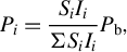
The lens system serves two primary functions: initializing ray directions and power, and placing rays at their intersection with the domain boundary while properly initializing their velocities. Two circular planes represent the focusing lens and focal spot, divided into subregions, each carrying a fraction of the spot energy:

(11) $$\begin{align}{P}_{i}=\frac{S_{i}{I}_{i}}{\Sigma {S}_{i}{I}_{i}}{P}_{\mathrm{b}},\end{align}$$

where ${P}_{i}$ is ray power, ${P}_{\mathrm{b}}$ is beam power, ${S}_{i}$ is subregion area and ${I}_{i}$ is intensity at the grid center. Subregion division methods include rectangular grids, polar coordinate grids and finite element grids. Figure 2(a) shows a rectangular division template for a super-Gaussian spot, with the red circle indicating the lens boundary. The lens and focal plane circles share the same division template, scaled according to their radii.

Figure 2 (a) Power partitioning of the laser focal spot. Intersection points (marked with ‘+’) of rays with (b) rectangular, (c) cylindrical and (d) spherical computational domains between the lens and focal planes.

Rays spawn at subregion centers, initially distributed in the $Z=0$ plane with a normal direction along $Z+$ . Rotation and translation are applied to position the rays on the user-defined 3D lens and focal planes. For a given polar angle ${\theta}_{\mathrm{B}}$ and azimuthal angle ${\phi}_{\mathrm{B}}$ of the line connecting the lens and focal plane centers, a corresponding 3D rotation is constructed:

$$\begin{align*} {\mathrm{\mathcal{R}}}_{\mathrm{B}}&=\left[\begin{array}{@{}ccc@{}}\mathit{\cos}\left(\pi +{\theta}_{\mathrm{B}}\right)& -\mathit{\sin}\left(\pi +{\theta}_{\mathrm{B}}\right)& 0\\ {}\mathit{\sin}\left(\pi +{\theta}_{\mathrm{B}}\right)& \mathit{\cos}\left(\pi +{\theta}_{\mathrm{B}}\right)& 0\\ {}0& 0& 1\end{array}\right]\\& \quad \times \left[\begin{array}{@{}ccc@{}}\mathit{\cos}\left(\pi /2+{\phi}_{\mathrm{B}}\right)& 0& \mathit{\sin}\left(\pi /2+{\phi}_{\mathrm{B}}\right)\\ {}0& 1& 0\\ {}-\mathit{\sin}\left(\pi /2+{\phi}_{\mathrm{B}}\right)& 0& \mathit{\cos}\left(\pi /2+{\phi}_{\mathrm{B}}\right)\end{array}\right].\end{align*}$$

In ${\mathrm{\mathcal{R}}}_{\mathrm{B}}$ , the second matrix performs a rotation around the Y-axis to adjust the inclination, followed by the first matrix rotating around the Z-axis to adjust the azimuth. The rotated points are then translated to position the rays on the lens and focal planes in 3D space.

Ray intersections with the computational domain mark the starting points for ray tracing, as illustrated in Figures 2(b)–2(d) with ‘+’ signs. In Cartesian coordinates, determining the starting points $\vec{i}$ is straightforward, as discussed in the cell-AVG introduction. However, this process becomes more complex in curvilinear coordinates. Given two points $\vec{T}$ (inside) and $\vec{L}$ (outside) relative to a surface of radius $r$ , the aiming vector from the lens to the focal plane is $\vec{a}=\vec{T}-\vec{L}$ . Here, vector components are denoted by subscripts (e.g., $\vec{a}=\left({a}_x,{a}_y,{a}_z\right)$ ), uppercase letters $X,Y,Z$ represent coordinate axes and $\left\Vert \vec{a}\right\Vert$ denotes the vector magnitude. The intersection-finding procedure preserves the curved geometry of radial cell faces, distinguishing it from methods used for co-planar TW-cell faces.

(I) For the cylindrical domain shown in Figure 3(a), construct the projection and rotation matrices:

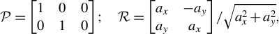(12) $$\begin{align}\mathcal{P}=\left[\begin{array}{@{}ccc@{}}1& 0& 0\\ {}0& 1& 0\end{array}\right];\quad \mathrm{\mathcal{R}}=\left[\begin{array}{@{}cc@{}}{a}_x& -{a}_y\\ {}{a}_y& {a}_x\end{array}\right]/\sqrt{a_x^2+{a}_y^2},\end{align}$$

where $\mathcal{P}$ represents a projection onto the X–Y plane, yielding ${\vec{T}}^{\prime}=\mathcal{P}\vec{T}$ , ${\vec{L}}^{\prime}=\mathcal{P}\vec{L}$ . Here, $\mathrm{\mathcal{R}}$ is a rotation in the X–Y plane aligning the unit vector $\left(1,0\right)$ to the direction $\left({a}_x,{a}_y\right)$ , while ${\mathrm{\mathcal{R}}}^{-1}$ rotates any $\left({a}_x,{a}_y\right)$ back to $\left(1,0\right)$ . This produces ${\vec{T}}^{{\prime\prime}}={\mathrm{\mathcal{R}}}^{-1}{\vec{T}}^{\prime }$ and ${\vec{L}}^{{\prime\prime}}={\mathrm{\mathcal{R}}}^{-1}{\vec{L}}^{\prime }$ . The points ${T}^{{\prime\prime} },{L}^{{\prime\prime} },{i}^{{\prime\prime} }$ are thus mapped onto the ‘solution plane’ shown in Figure 3(c), where the line connecting these points is guaranteed to be parallel to the local ${X}^{{\prime\prime} }$ -axis, allowing the intersection point coordinates ${i}^{{\prime\prime} }$ to be directly determined:

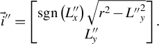(13) $$\begin{align}{\vec{i}}^{{\prime\prime}}=\left[\begin{array}{@{}c@{}}\mathit{\operatorname{sgn}}\left({L}_x^{{\prime\prime}}\right)\sqrt{r^2-{L^{{\prime\prime}}}_y^2}\\ {}{L}_y^{{\prime\prime}}\end{array}\right].\end{align}$$

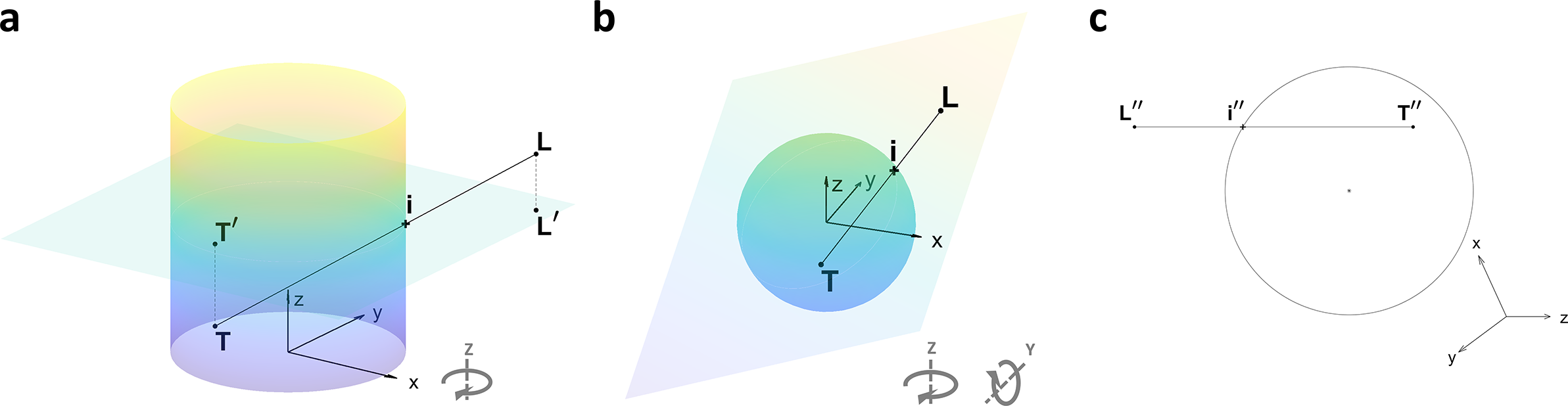
Figure 3 (a) Intersection of the connecting line with a cylindrical surface, where $\vec{T}$ and $\vec{L}$ are projected onto the solution plane followed by a Z-rotation. (b) Intersection of the connecting line with a spherical surface, where $\vec{T}$ and $\vec{L}$ are mapped to the solution plane through a Z-rotation followed by a Y-rotation. (c) In solution plane, the line connecting ${T}^{{\prime\prime} },\ {L}^{{\prime\prime} }$ and ${i}^{{\prime\prime} }$ is parallel to the X-axis, enabling straightforward calculation of the intersection point ${i}^{{\prime\prime} }$ coordinates.

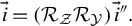
Rotating ${i}^{{\prime\prime} }$ back and scaling along the aiming vector $\vec{a}$ gives the intersection point in the fluid reference frame:

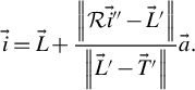(14) $$\begin{align}\vec{i}=\vec{L}+\frac{\left\Vert \mathrm{\mathcal{R}}{\vec{i}}^{{\prime\prime} }-{\vec{L}}^{\prime}\right\Vert }{\left\Vert {\vec{L}}^{\prime }-{\vec{T}}^{\prime}\right\Vert}\vec{a}.\end{align}$$

For cylindrical domains, additional considerations are necessary. Firstly, rays may intersect the flat faces of the cylinder. The scaling factors to the top and bottom faces are $\mid \left({L}_z-{Z}_{\mathrm{max}}\right)/\left({T}_z-{L}_z\right)\mid$ and $\mid \left({T}_z-{Z}_{\mathrm{min}}\right)/\left({T}_z-{L}_z\right)\mid$ , respectively. The minimum of these three factors, including the one for the curved surface, should be chosen to scale $\vec{a}$ , as the true intersection is the closest to the lens. Secondly, when laser incidence aligns with the cylindrical axis ( $\sqrt{a_x^2+{a}_y^2}=0$ ), the rotation matrix $\mathrm{\mathcal{R}}$ must be set to the identity matrix $\mathrm{\mathcal{I}}$ to avoid singularity.

(II) For the spherical domain shown in Figure 3(b), two rotation matrices are constructed:

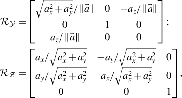$$\begin{align*}{\mathrm{\mathcal{R}}}_{\mathcal{Y}}&=\left[\begin{array}{@{}ccc@{}}\sqrt{a_x^2+{a}_y^2}/\left\Vert \vec{a}\right\Vert & 0& -{a}_z/\left\Vert \vec{a}\right\Vert \\ {}0& 1& 0\\ {}{a}_z/\left\Vert \vec{a}\right\Vert & 0& 0\end{array}\right];\\{\mathrm{\mathcal{R}}}_{\mathcal{Z}}&=\left[\begin{array}{@{}ccc@{}}{a}_x/\sqrt{a_x^2+{a}_y^2}& -{a}_y/\sqrt{a_x^2+{a}_y^2}& 0\\ {}{a}_y/\sqrt{a_x^2+{a}_y^2}& {a}_x/\sqrt{a_x^2+{a}_y^2}& 0\\ {}0& 0& 1\end{array}\right], \end{align*}$$

where ${\mathrm{\mathcal{R}}}_{\mathcal{Y}}$ represents a rotation around the Y-axis by the polar angle of the connecting line, and ${\mathrm{\mathcal{R}}}_{\mathcal{Z}}$ represents a rotation around the Z-axis by its azimuth angle. Applying these rotations to the points $\vec{L},\vec{T}$ gives ${\vec{T}}^{{\prime\prime}}={\left({\mathrm{\mathcal{R}}}_{\mathcal{Z}}{\mathrm{\mathcal{R}}}_{\mathcal{Y}}\right)}^{-1}\vec{T}$ , ${\vec{L}}^{{\prime\prime}}={\left({\mathrm{\mathcal{R}}}_{\mathcal{Z}}{\mathrm{\mathcal{R}}}_{\mathcal{Y}}\right)}^{-1}\vec{L}$ . The intersection point coordinates are then determined on the solution plane as follows:

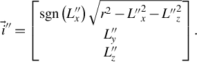(15) $$\begin{align}{\vec{i}}^{{\prime\prime}}=\left[\begin{array}{@{}c@{}}\mathit{\operatorname{sgn}}\left({L}_x^{{\prime\prime}}\right)\sqrt{r^2-{L^{{\prime\prime}}}_x^2-{L^{{\prime\prime}}}_z^2}\\ {}{L}_y^{{\prime\prime}}\\ {}{L}_z^{{\prime\prime}}\end{array}\right].\end{align}$$

Rotating ${i}^{{\prime\prime} }$ back to the fluid reference frame gives the spherical intersection:

(16) $$\begin{align}\vec{i}=\left({\mathrm{\mathcal{R}}}_{\mathcal{Z}}{\mathrm{\mathcal{R}}}_{\mathcal{Y}}\right){\vec{i}}^{{\prime\prime} }.\end{align}$$

This establishes the ray starting points on the domain boundary. Alternatively, starting points can be determined by solving the quadratic equation of a line and a curved surface. However, matrix operations are more compact and efficient due to simplification and pre-evaluation. They also enable highly vectorized data flows, leveraging modern hardware for improved performance.

Finally, the ray velocity must be properly initialized, as rays may originate inside the plasma corona. The velocity magnitude is determined by the local refractive index $N$ , where ${v}_0= cN=c\sqrt{1-{n}_{\mathrm{e}}/{n}_{\mathrm{c}}}$ . The velocity direction is aligned with the aiming vector, given by ${v}_{0x}={cNa}_x/\left\Vert \vec{a}\right\Vert, {v}_{0y}={cNa}_y/\left\Vert \vec{a}\right\Vert, {v}_{0z}={cNa}_z/\left\Vert \vec{a}\right\Vert$ .

3.2 Field interpolation

Ray advancement requires the field value at each node in space. The general principle of interpolation is to ensure continuity and minimize oscillation. Testing has shown that linear (1D), bilinear (2D) and trilinear (3D) interpolation schemes are optimal for this purpose.

For clarity, a 2D bilinear interpolation case is illustrated in Figure 4(a). Cell edge lengths are $\Delta x,\Delta y$ , with $V$ as the base value at the cell vertex. The distances from the interior sampling point $S$ to cell walls are $x,y$ :

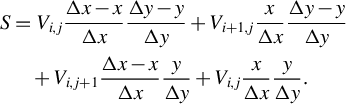$$\begin{align*}S&={V}_{i,j}\frac{\Delta x-x}{\Delta x}\frac{\Delta y-y}{\Delta y}+{V}_{i+1,j}\frac{x}{\Delta x}\frac{\Delta y-y}{\Delta y}\\& \quad +{V}_{i,j+1}\frac{\Delta x-x}{\Delta x}\frac{y}{\Delta y}+{V}_{i,j}\frac{x}{\Delta x}\frac{y}{\Delta y}.\end{align*}$$

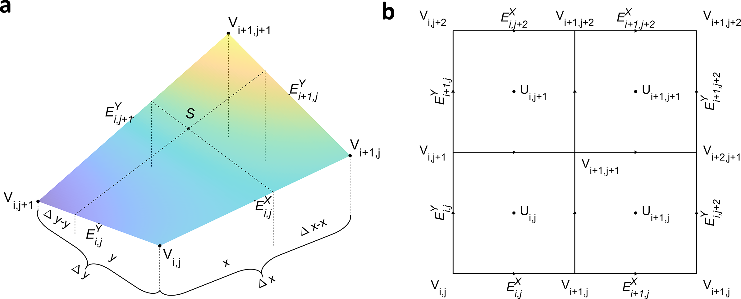
Figure 4 (a) Bilinear interpolation for interior point $S$ ’s value and spatial derivatives. Region dimensions are $\Delta x,\Delta y$ , with $S$ coordinates $x,y$ (origin at the lower-left corner). Here, $V$ represents cell vertex values and ${E}^X,{E}^Y$ are edge-centered gradients. (b) Vertex values $V$ and edge gradients ${E}^X,{E}^Y$ are derived from known cell-centered values $U$ .

Interpolation weights for each vertex are proportional to the areas of the quadrilaterals opposite them. Notably, despite the term ‘linear’, interpolated fine meshes are generally not planar, as shown in Figure 4(a). Since bilinear and trilinear interpolations ensure continuity across cells, rays crossing cell boundaries do not require total reflection checks.

Field gradients are essential for advancing the ray and are calculated as follows:

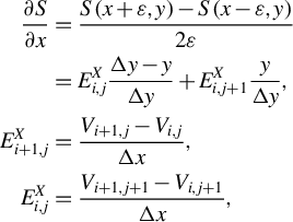$$\begin{align*} \frac{\partial S}{\partial x}&=\frac{S\left(x+\varepsilon, y\right)-S\left(x-\varepsilon, y\right)}{2\varepsilon}\\&={E}_{i,j}^X\frac{\Delta y-y}{\Delta y}+{E}_{i,j+1}^X\frac{y}{\Delta y},\\{E}_{i+1,j}^X&=\frac{V_{i+1,j}-{V}_{i,j}}{\Delta x},\\{E}_{i,j}^X&=\frac{V_{i+1,j+1}-{V}_{i,j+1}}{\Delta x},\end{align*}$$

where $\varepsilon$ is a small step size, ${E}_{i,j},{E}_{i,j+1}$ are gradient values at edge centers and superscripts denote direction. The derivation shows that the gradient at any point within the cell is a linear combination of edge-centered gradients. The expression for $\partial S/\partial y$ takes a similar form, with indices appropriately interchanged.

For specific ray-tracing tasks, physical quantities relevant to laser trajectories and energy deposition – such as density, temperature and effective charge state – are required. As shown in Figure 4(b), these fluid quantities are defined at cell centers, denoted as $U$ . During domain initialization, cell-center interpolation is used to compute vertex values $V$ (outermost extrapolated vertices take the nearest cell-center values). Edge-centered gradients ${E}^X$ , ${E}^Y$ are then calculated by dividing vertex value differences by edge lengths $\Delta x,\Delta y$ .

Piecewise linear interpolation does not ensure continuity of first-order derivatives, leading to the question: why not use higher-order interpolation schemes? Higher-order methods, however, are unsuitable for ray tracing in plasma due to severe Runge phenomena. Figure 5 demonstrates this issue using a rarefaction wave field with known values (black asterisks). Piecewise cubic interpolation is compared to linear interpolation. The cubic interpolation assumes an intra-cell field form $S(x)={a}_0+{a}_1x+{a}_2{x}^2+{a}_3{x}^3$ , where coefficients ${a}_{0}{-}{a}_{3}$ are determined by four conditions: field values $S(0),S(1)$ and gradient values $\partial S(0)/\partial x,\partial S(1)/\partial x$ at cell corners.

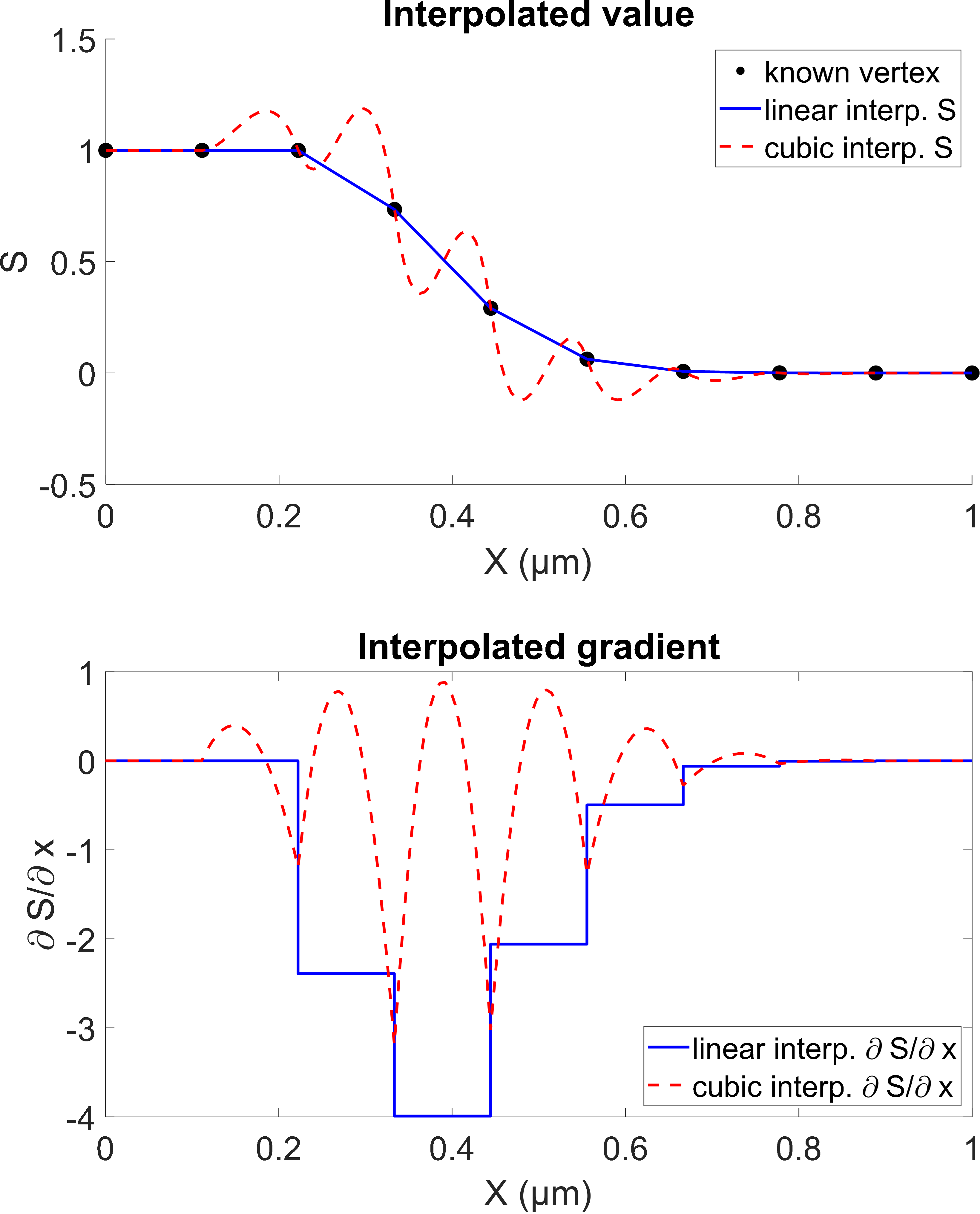
Figure 5 Comparison of linear interpolation and cubic interpolation methods for constructing internal field values $S$ and gradient values $\partial S/\partial x$ of a rarefaction wave.

Although cubic interpolation ensures continuity of first-order spatial derivatives, it introduces substantial oscillations, which worsen with cell refinement. Such oscillations can even produce negative values for inherently positive physical quantities, as shown in Figure 5. This leads to incorrect ray refraction locations, making higher-order methods unreliable for this application. In contrast, bilinear/trilinear interpolation offers superior robustness. When combined with adaptive-step RK methods, the lack of first-order derivative continuity does not significantly affect ray-tracing accuracy.

3.3 Adaptive ray stepping

The ray trajectories are solved using the RKF method with adaptive step size. Like all RK methods, the RKF method approximates ray curves through a straight-line segments sequence ordered according to the time parameter $t$ . The advantage of the RKF method lies in its dynamic adjustment of the step size $\Delta t$ , allowing larger steps in regions with gradual field variations and smaller steps in regions with sharp refraction. In plasmas, where the refractive index distribution is highly nonuniform, adaptive step sizing can often reduce computational costs by one to two orders of magnitude. The system of ordinary differential equations for ray trajectories is as follows:

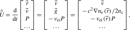(17) $$\begin{align}\dot{\vec{U}}=\frac{\mathrm{d}}{\mathrm{d}t}\left[\begin{array}{@{}c@{}}\vec{r}\\ {}\vec{v}\\ {}P\\ {}\dots \end{array}\right]=\left[\begin{array}{@{}c@{}}\vec{v}\\ {}\vec{g}\\ {}-{\nu}_{\mathrm{ei}}P\\ {}\dots \end{array}\right]=\left[\begin{array}{@{}c@{}}\vec{v}\\ {}-{c}^2\nabla {n}_{\mathrm{e}}\left(\vec{r}\right)/2{n}_{\mathrm{c}}\\ {}-{\nu}_{\mathrm{ei}}\left(\vec{r}\right)P\\ {}\dots \end{array}\right],\end{align}$$

where $\vec{U}$ represents the solution vector, ray acceleration is $\vec{g}=\vec{f}/m$ with $m=1$ , $P$ denotes ray power and ${\nu}_{\mathrm{ei}}$ is the absorption coefficient, calculated via field interpolation. The ellipsis indicates other physical quantities varying along the ray path. The RK4(5) coefficients from Fehlberg’s original work^{[ 28 ]} are used to estimate the solution gradient at the initial condition ${\vec{U}}^n$ :

$$\begin{align*}{\vec{k}}_1&={\dot{\vec{U}}}_n\left({\vec{r}}_0\right),\\{\vec{k}}_2&={\dot{\vec{U}}}_n\left({\vec{r}}_0\right)+\left(2/9\right){\vec{k}}_1\Delta t,\\{\vec{k}}_3&={\dot{\vec{U}}}_n\left({\vec{r}}_0\right)+\left(\left(1/12\right){\vec{k}}_1+\left(1/4\right){\vec{k}}_2\right)\Delta t,\\{\vec{k}}_4&={\dot{\vec{U}}}_n\left({\vec{r}}_0\right)+\Big(\left(69/128\right){\vec{k}}_1+\left(-243/128\right){\vec{k}}_2\\& \quad +\left(135/64\right){\vec{k}}_3\Big)\Delta t,\\{\vec{k}}_5&={\dot{\vec{U}}}_n\left({\vec{r}}_0\right)+\Big(\left(-17/12\right){\vec{k}}_1+\left(27/4\right){\vec{k}}_2\\& \quad +\left(-27/5\right){\vec{k}}_3+\left(16/15\right){\vec{k}}_4\Big)\Delta t,\\{\vec{k}}_6&={\dot{\vec{U}}}_n\left({\vec{r}}_0\right)+\Big(\left(65/432\right){\vec{k}}_1+\left(-5/16\right){\vec{k}}_2\\& \quad +\left(13/16\right){\vec{k}}_3+\left(4/27\right){\vec{k}}_4+\left(5/144\right){\vec{k}}_5\Big)\Delta t.\end{align*}$$

The RKF method estimates the single-step error by comparing the solution difference between fourth- and fifth-order approximations:

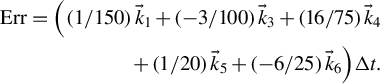$$\begin{align*} \mathrm{Err}=\Big(\left(1/150\right){\vec{k}}_1+\left(-3/100\right){\vec{k}}_3+\left(16/75\right){\vec{k}}_4\\ {}\kern3em +\left(1/20\right){\vec{k}}_5+\left(-6/25\right){\vec{k}}_6\Big)\Delta t.\end{align*}$$

If the error is below the tolerance $\mathrm{Tol}$ , this step is accepted, producing ${\vec{U}}_{n+1}$ for the next time step:

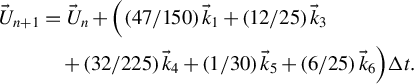$$\begin{align*}{\vec{U}}_{n+1}&={\vec{U}}_n+\Big(\left(47/150\right){\vec{k}}_1+\left(12/25\right){\vec{k}}_3\\& \quad +\left(32/225\right){\vec{k}}_4+\left(1/30\right){\vec{k}}_5+\left(6/25\right){\vec{k}}_6\Big)\Delta t.\end{align*}$$

The time step is dynamically adjusted as follows:

$$\begin{align*}\Delta {t}_{\mathrm{new}}=C\Delta t{\left( \mathrm{Err}/ \mathrm{Tol}\right)}^{1/5}.\end{align*}$$

The default safety factor is $C=0.9$ . The initial step size can be conservatively estimated as $\Delta {t}_{\mathrm{init}.}=0.5N\Delta X/c$ ( $\Delta X$ is the cell edge length). For accepted steps, the step size increases but is capped at $\Delta {t}_{\mathrm{max}}=\Delta X/c$ to ensure the ray does not cross more than two cells per coordinate direction in a single RK step. If the tolerance is not met, the calculation restarts from ${\vec{U}}_n$ with progressively smaller trial step sizes.

While not the fastest in convergence, Fehlberg’s original coefficients offer the advantage of using non-negative weights for slope combinations, preserving the sign of physical quantities. For instance, predicted changes in ray power remain negative, maintaining physical consistency.

The adaptive RKF method naturally incorporates energy absorption into error control. However, a special case arises where RKF advancement may produce incorrect nodes despite satisfying the error tolerance, as shown in Figure 6. This typically occurs at density discontinuities near solid target surfaces. All six RKF midpoint evaluations may lie entirely within the low-density region, causing the ray to erroneously overshoot into the super-critical density region instead of reflecting at the interface.

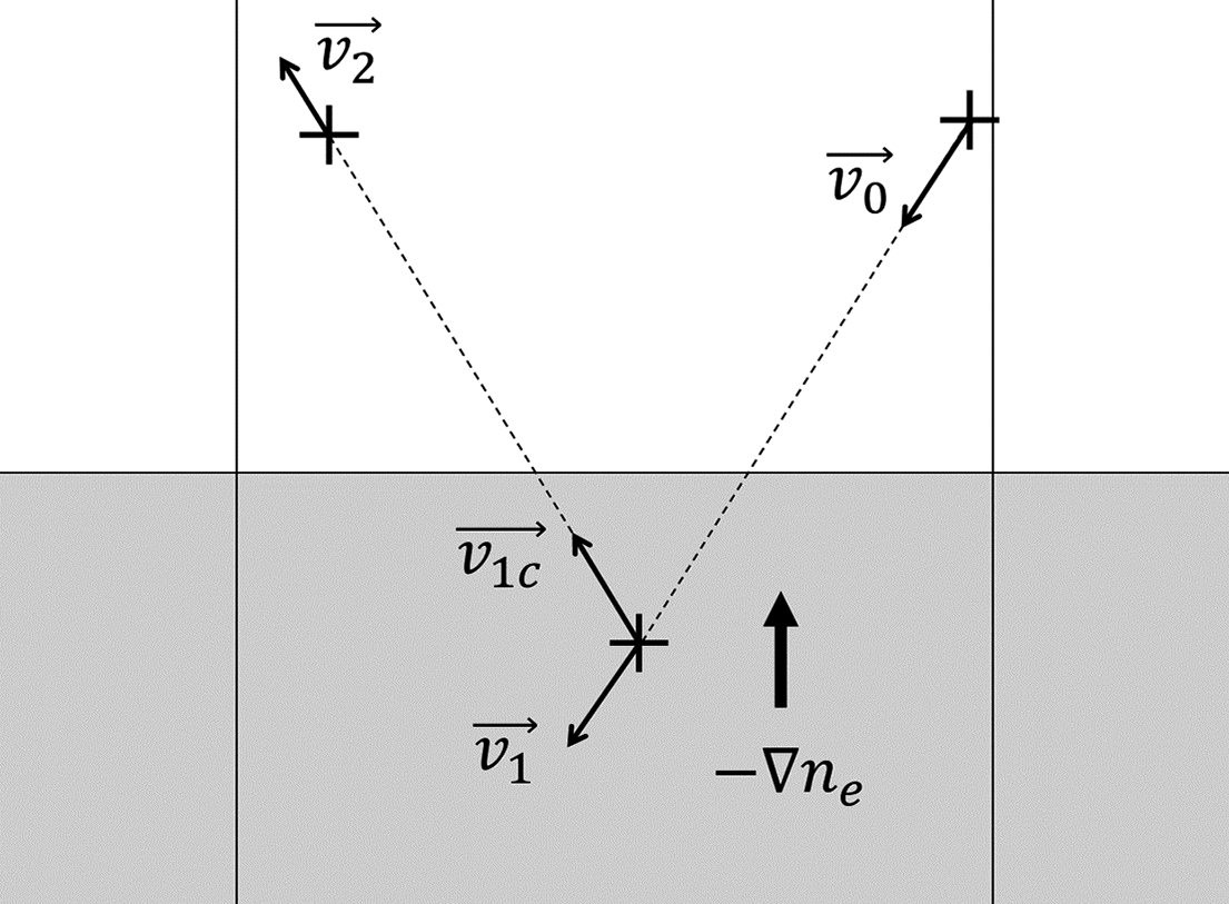
Figure 6 Ray reflection at a sharp interface. The lower part represents the high-density target. Here, ${\vec{v}}_0$ is the incident velocity, ${\vec{v}}_1$ the overshoot velocity, ${\vec{v}}_{1\mathrm{c}}$ the corrected velocity and ${\vec{v}}_2$ the ejection velocity.

At sharp interfaces, extremely small RK steps would be needed to accurately capture trajectory curves, which is computationally inefficient and physically unrealistic. RKF failure can also be identified by violations of energy conservation at nodes ( $v/c\ne N$ ). To address this, a velocity correction patch is applied when energy conservation is violated:

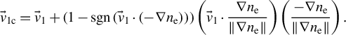$$\begin{align*}{\vec{v}}_{1\mathrm{c}}={\vec{v}}_1+\left(1-\mathit{\operatorname{sgn}}\left({\vec{v}}_1\cdot \left(-\nabla {n}_{\mathrm{e}}\right)\right)\right)\left({\vec{v}}_1\cdot \frac{\nabla {n}_{\mathrm{e}}}{\left\Vert \nabla {n}_{\mathrm{e}}\right\Vert}\right)\left(\frac{-\nabla {n}_{\mathrm{e}}}{\left\Vert \nabla {n}_{\mathrm{e}}\right\Vert}\right).\end{align*}$$

This patch reflects the ray velocity ${\vec{v}}_1$ to ${\vec{v}}_{1\mathrm{c}}$ if it forms an obtuse angle with the acceleration direction $-\nabla {n}_{\mathrm{e}}$ , bending it back toward the lower-density region. No correction is applied for acute angles. This patch is particularly important during the initial simulation frames and becomes unnecessary once plasma spans several cells.

The number of RKF steps for a single ray is approximately proportional to the cell count in the fluid domain, ensuring computational efficiency.

3.4 Rasterized deposition

The rasterization process handles individual RK line segments to allocate energy losses, as illustrated in Figure 7, which shows possible relative positions between line segments and 2D fluid cells:

1. (1) no crossing;

2. (2) single-cell-face crossing (X or Y);

3. (3) double-cell-face crossing (X–Y/Y–X).

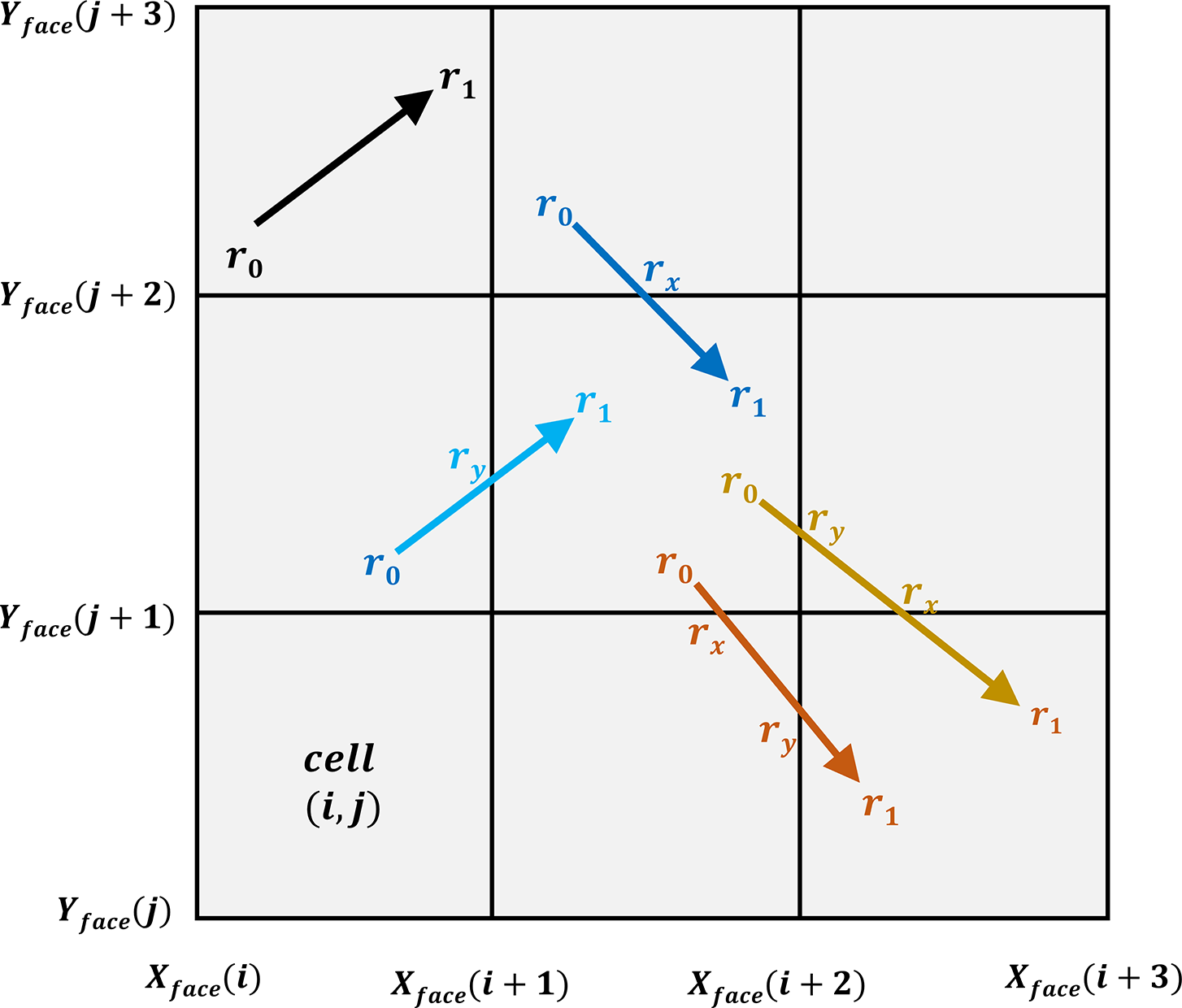
Figure 7 Possible scenarios of ray segments intersecting 2D fluid cells under the $\Delta {t}_{\mathrm{max}}=\Delta x/c$ constraint. Rectangular faces are shown, but sphere/cylinder faces are also applicable.

When a line segment is divided into subsegments $\Delta {l}_1,\Delta {l}_2,\dots \left(\Delta t=\Delta {t}_1+\Delta {t}_2+\dots \right)$ by cell faces, the single-step energy deposition is distributed among subsegments as $\Delta {P}_1\propto {\overline{\nu}}_{\mathrm{ei}}P\Delta {t}_1,\Delta {P}_2\propto {\overline{\nu}}_{\mathrm{ei}}P\Delta {t}_2,\dots$ , and so on. Since ray acceleration $\overline{g}$ remains constant within a single RK step, subsegment lengths can be expressed as $\Delta {l}_1=v\Delta {t}_1+0.5\overline{g}\Delta {t}_1^2,\Delta {l}_2=\left(v+\overline{g}\Delta {t}_1\right)\Delta {t}_2+0.5\overline{g}\Delta {t}_2^2,\dots$ . The RKF method ensures $v>\overline{g}\Delta t$ everywhere except at normal-incidence reflection points. Neglecting higher-order terms of time, the approximation $\Delta {P}_1:\Delta {P}_2\approx \Delta {l}_1:\Delta {l}_2$ indicates that energy deposition ratios across cells are proportional to subsegment lengths.

For 1D energy deposition, as shown in the flowchart in Figure 8, the process involves the following steps: given line segment endpoints ${\vec{r}}_0,{\vec{r}}_1$ and their corresponding cell indices ${i}_0,{i}_1$ , potential cell face intersections are determined as ${\vec{r}}_x={X}_{\mathrm{face}}\left(\mathit{\max}\left({i}_0,{i}_1\right)\right)$ regardless of the ray’s traveling direction. The array ${X}_{\mathrm{face}}$ stores the coordinates of all cell faces. If ${r}_0={r}_1$ , indicating no crossing, the ray’s energy loss is entirely deposited in local cell ${i}_0$ . Otherwise, the energy is distributed between adjacent cells ${i}_0$ and ${i}_1$ in proportion to the subsegment lengths.

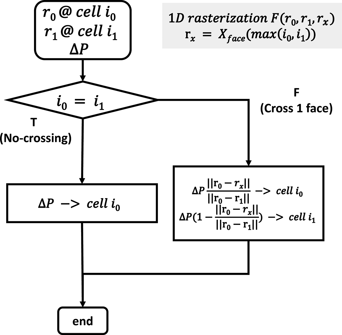
Figure 8 One-dimensional energy deposition rasterization allocation process.

For 2D energy deposition, as outlined in the flowchart in Figure 9, the process begins by determining 2D cell indices ${i}_0,{j}_0,{i}_1,{j}_1$ from the endpoint coordinates ${\vec{r}}_0,{\vec{r}}_1$ . The algorithm proceeds with branch case evaluation:

1. (1) no crossing?

2. (2) single X-face crossing?

3. (3) single Y-face crossing?

4. (4) double-face crossing?

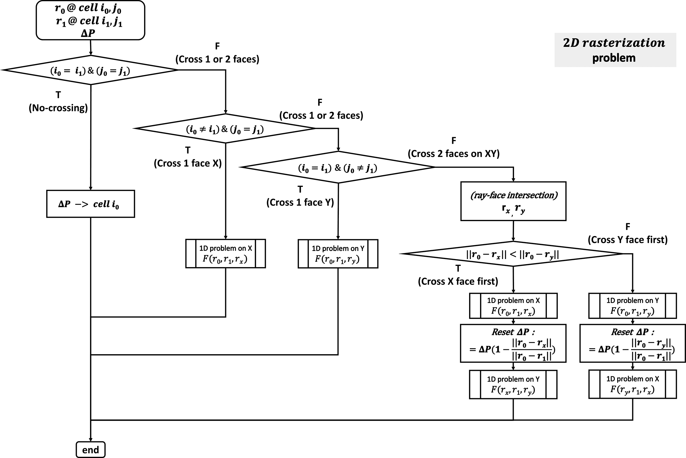
Figure 9 Two-dimensional energy deposition rasterization process.

The first three cases reduce to 1D problems along the X- or Y -direction. For the fourth case (double-face crossing), intersections ${\vec{r}}_x,{\vec{r}}_y$ with X/Y faces are calculated using the same line–face intersection subroutine from the ‘lens system’ to determine the first intersected face.

1. (1) If the X-face is encountered first, the X-direction 1D problem is solved, then the starting point is updated ${\vec{r}}_0\to {\vec{r}}_x$ and the Y-direction problem is solved with the remaining energy $\Delta P$ .

2. (2) If the Y-face is encountered first, the same logic applies, but in reverse order.

This approach ensures that 2D problems are always decomposed into a sequence of 1D solutions for computational simplicity and efficiency.

While the flowchart for 3D fluid cell energy allocation would be extensive, the actual implementation is concise. 1D problems involve two branches, 2D problems have four and 3D problems can be treated as an eight-branch structure using two-layer decompositions: 3D to 2D, and 2D to 1D. All branches ultimately reduce to 1D problems, allowing recursive logic to efficiently construct energy allocation algorithms for any dimension.

Volume-averaged quantities, such as frequency shifts and polarization, can be computed using the same rasterization logic. By weighting with ray power first and then depositing onto cells, these quantities are easily calculated. For flux density, such as light intensity $I$ , ray power through cell faces is tracked. At each interface crossing, ray power $P$ is accumulated into the entered cell ${i}_1$ . The intensity is then calculated as ${I}_{\mathrm{cell}}={\Sigma}_{\mathrm{cross}}{P}_{\mathrm{ray}}/{S}_{\mathrm{proj}}$ , where the projected area ${S}_{\mathrm{proj}}=\mathit{\cos}\left(\mathit{\min}\left(\theta, \pi /2-\theta \right)\right)\Delta X\Delta Y$ (in two dimensions), and $\theta$ is the angle between the ray and the cell face normal.

This concludes the description of an unconstrained, rasterization-based algorithm for ray tracing in gradient-index media. Aside from adaptive RK step-size adjustments, the algorithm is non-iterative and employs a unified tracing kernel applicable to all coordinate systems.

4 Test cases for rasterized ray tracing

4.1 Plasma Luneburg lens (ray 3D-in-1D sphere)

The Luneburg lens^{[ 32 ]} is a spherical lens with a refractive index that gradually decreases from the center to the periphery. Parallel incident rays focus to a point on the lens surface, while a point source at the boundary produces parallel rays on the opposite side. This property makes the Luneburg lens ideal for beam forming and directional radiation applications. The refractive index distribution of a classical optical Luneburg lens is given by

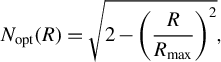$$\begin{align*}{N}_{\mathrm{opt}}(R)=\sqrt{2-{\left(\frac{R}{R_{\mathrm{max}}}\right)}^2},\end{align*}$$

where $R$ is the radial coordinate of the spherical lens, with the refractive index ${N}_{\mathrm{opt}}$ maximized at the center and equal to unity at the boundary ${R}_{\mathrm{max}}$ .

Plasma refractive indices are inherently less than unity. However, it is possible to construct a ‘plasma Luneburg lens’ with equivalent focusing performance (for extended designs, see Ref. [33]). The refractive index distribution for a plasma Luneburg lens is given by the following:

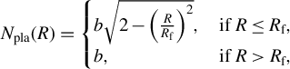(18) $$\begin{align}{N}_{\mathrm{pla}}(R)=\left\{\begin{array}{@{}ll@{}}b\sqrt{2-{\left(\frac{R}{R_{\mathrm{f}}}\right)}^2},& \mathrm{if}\;R\leq{R}_{\mathrm{f}},\\{}b, &\mathrm{if}\;R>{R}_{\mathrm{f}},\end{array}\right.\end{align}$$

where $b\in \left[1,1/\sqrt{2}\right]$ is a scaling factor, and ${R}_{\mathrm{f}}<{R}_{\mathrm{max}}$ is the focal sphere radius. The corresponding electron density distribution is as follows:

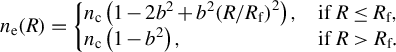(19) $$\begin{align}{n}_{\mathrm{e}}(R)=\left\{\begin{array}{@{}ll@{}}{n}_{\mathrm{c}}\left(1-2{b}^2+{b}^2{\left(R/{R}_{\mathrm{f}}\right)}^2\right),& \mathrm{if}\;R\leq{R}_{\mathrm{f}},\\{}{n}_{\mathrm{c}}\left(1-{b}^2\right),& \mathrm{if}\;R>{R}_{\mathrm{f}}.\end{array}\right. \end{align}$$

Figure 10 presents an example within a spherical computational domain of $600\;\mu \mathrm{m}$ diameter. A parallel beam ( $\varPhi =400\;\mu \mathrm{m}$ ) is incident obliquely from above and focuses at $0.8{R}_{\mathrm{max}}$ on the opposite side.

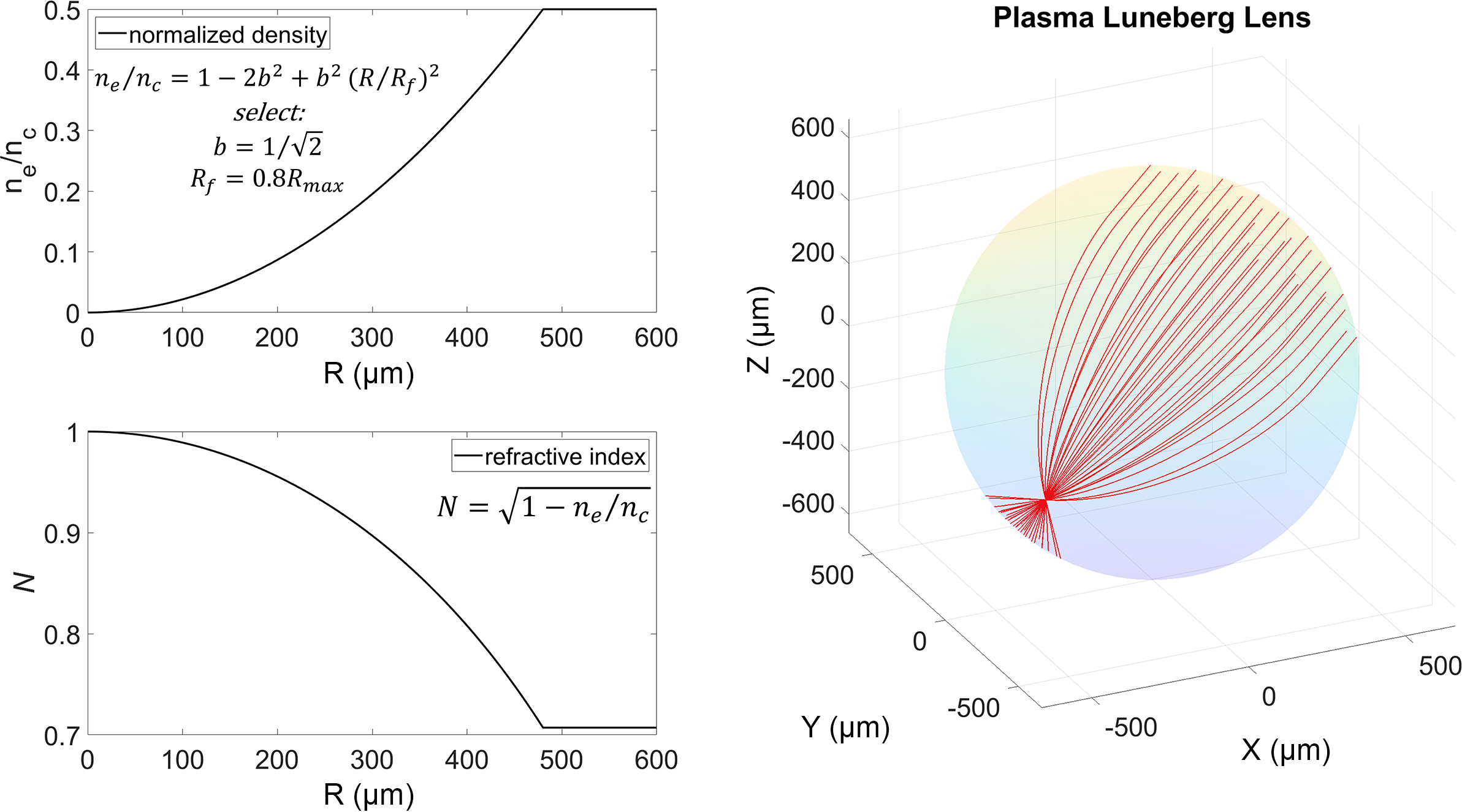
Figure 10 Plasma Luneburg lens parameters and ray trajectories.

The plasma Luneburg lens provides a precision benchmark for ray-tracing algorithms. As shown in Figure 11(a), a grid with $\Delta X=3\;\mu \mathrm{m}$ (200 cells along $R$ ) achieves a focal spot smaller than $0.05\;\mu \mathrm{m}$ in diameter. Errors, primarily from field interpolation and RK stepping, decrease with grid refinement. A grid spacing scan from $0.375$ to $12\;\mu \mathrm{m}$ produces the error statistics in Figure 11(b).

1. (1) The residual ${\Sigma}_{ij,i>j}\left(\left\Vert {\vec{r}}_{\mathrm{i}}-{\vec{r}}_j\right\Vert \right)/{C}_{n_{\mathrm{ray}}}^2$ , defined as the average distance between impact points $i,\ j,\ k,\dots$ , converges at $\mathcal{O}\left(\Delta {X}^2\right)$ .

2. (2) The root mean square (RMS) of impact point distribution shows exponential convergence, indicating a significantly higher ray density at the focal spot center compared to the surrounding halo.

This highlights the algorithm’s precision and its efficiency in capturing fine-scale focusing behavior.

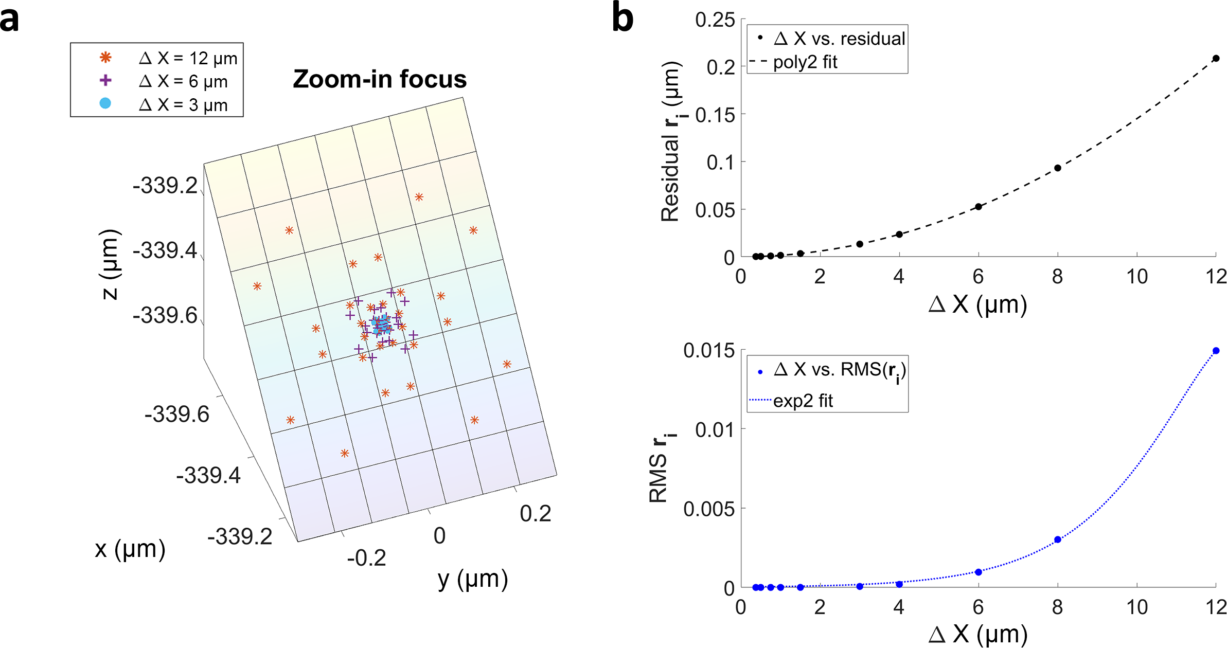
Figure 11 (a) Ray impact points near the focus. Shown are 32 rays per beam. (b) Error in impact point distribution versus cell grid spacing.

4.2 Plasma Doppler shift (ray 3D-in-2D plane)

When laser light propagates in the plasma, Doppler frequency shifts occur due to plasma motion^{[ 34 ]}. These Doppler shifts influence the characteristics of laser–plasma interactions. In the fluid reference frame, the light wave frequency can be interpreted as the number of electric field peaks detected per unit time by a probe at the cell center: blue shifts occur when the phase velocity in plasma shows an increasing trend (analogous to an accelerating wave-peak conveyor) or when reflecting surfaces move toward the wave source, resulting in more wave peaks detected per unit time; red shifts occur under the opposite conditions. The Doppler frequency shift is quantitatively described by the following:

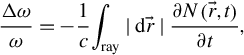(20) $$\begin{align}\frac{\Delta \omega }{\omega}=-\frac{1}{c}{\int}_{\mathrm{{\kern-5pt}ray}}\mid \mathrm{d}\vec{r}\mid \frac{\partial N\left(\vec{r},t\right)}{\partial t},\end{align}$$

where $\omega$ is the central frequency. Integration along the ray path provides the frequency shift at any location, assuming the shift is small relative to the central frequency. Using the fluid continuity equation, the rate of change of the refractive index can be expressed in terms of the flow field divergence:

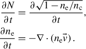$$\begin{align*}\frac{\partial N}{\partial t}&=\frac{\partial \sqrt{1-{n}_{\mathrm{e}}/{n}_{\mathrm{c}}}}{\partial t},\\\frac{\partial {n}_{\mathrm{e}}}{\partial t}&=-\nabla \cdot \left({n}_{\mathrm{e}}\vec{v}\right). \end{align*}$$

The frequency shift in a fluid cell is calculated as the power-weighted average of all incident rays:

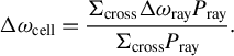(21) $$\begin{align}\Delta {\omega}_{\mathrm{cell}}=\frac{\Sigma_{\mathrm{cross}}\Delta {\omega}_{\mathrm{ray}}{P}_{\mathrm{ray}}}{\Sigma_{\mathrm{cross}}{P}_{\mathrm{ray}}}.\end{align}$$

Figure 12 shows Doppler frequency shifts in a 2D planar rarefaction wave. Using the ideal gas equation of state for fully ionized hydrogen plasma, the density and velocity follow self-similar solutions:

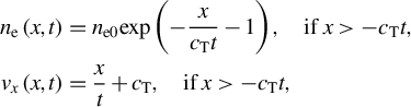$$\begin{align*}{n}_{\mathrm{e}}\left(x,t\right)&={n}_\mathrm{e0}\mathit{\exp}\left(-\frac{x}{c_\mathrm{T}t}-1\right),\quad \mathrm{if}\;x>-{c}_\mathrm{T}t,\\{v}_x\left(x,t\right)&=\frac{x}{t}+{c}_{\mathrm{T}},\quad \mathrm{if}\;x>-{c}_\mathrm{T}t,\end{align*}$$

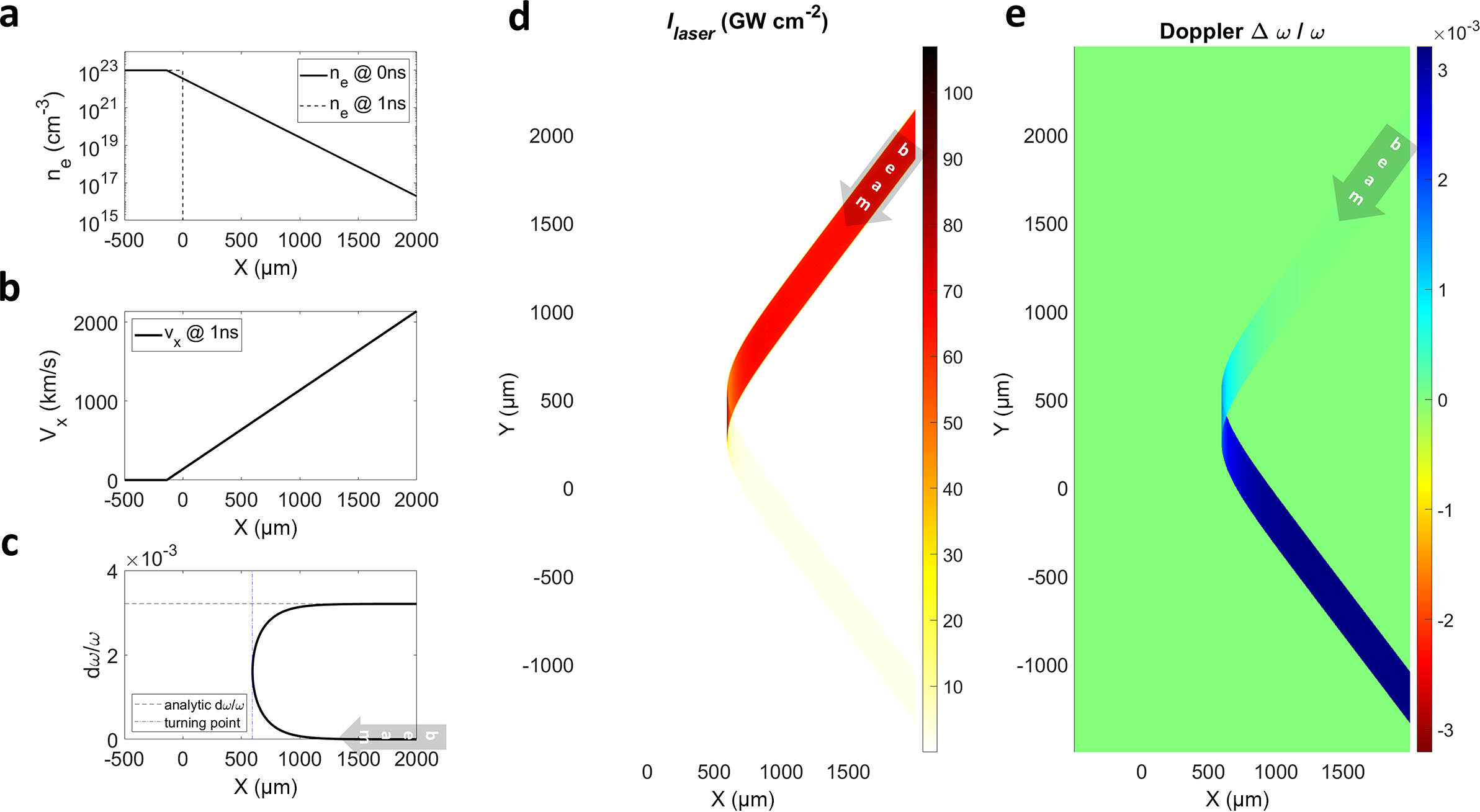
Figure 12 (a) Density and (b) flow velocity distributions of rarefied step-profile plasma. (c) Doppler frequency shifts during ray traversal through plasma. (d) Fluid domain light intensity. (e) Fluid domain frequency shift.

where ${c}_{\mathrm{T}}$ is the sound speed. For a step density ${n}_{\mathrm{e}0}=100{n}_{\mathrm{c}}$ , temperature ${T}_0=100\;\mathrm{eV}$ , and 1 ns rarefaction time, a $\lambda =1064\;\mathrm{nm}$ beam is incident at 45° from the right-hand boundary. Figure 12(c) depicts the frequency shift along the ray path. At a fluid cell spacing of $\Delta X=3.125\;\mu \mathrm{m}$ , ray tracing predicts $\Delta \omega /\omega =3.2069\times {10}^{-3}$ , corresponding to a wavelength shift of . The analytical solution (Equation (6) in Ref. [34]), $\Delta \omega /\omega =\left(2 \mathrm{cos}\theta /c\right)\left({v}_{\mathrm{TP}}+2\left(1-\mathit{\ln}2\right){c}_{\mathrm{T}}\right)$ , gives , where ${v}_{\mathrm{TP}}$ is the turning point velocity. The relative error is approximately ${10}^{-4}$ .

The Doppler shift is dominated by the near-critical to super-critical density transition region near the turning point. Accurate results require smooth ray trajectories in this region. In the cell-AVG algorithm, the density is discontinuous at the cell interface, leading to frequency shift errors up to 18% under identical conditions.

Figure 12(d) shows the fluid domain light intensity, with an incident power density of approximately $100\;\mathrm{GW}/{\mathrm{cm}}^2$ and about 95% energy absorption by the plasma. Figure 12(e) presents the frequency shift distribution in the fluid domain, indicating an overall blue shift after reflection.

4.3 Laser-driven gas sphere (ray 3D-in-2D cylinder)

The rasterization algorithm has been integrated into the multiphase RHD code DRIM (details to be published). A full-physics simulation of a laser-driven gas sphere demonstrates the robustness and efficiency of the laser module. The laser parameters are: $1064\;\mathrm{nm}$ wavelength, $80\;\mu \mathrm{m}$ focal spot diameter and $0.5\;\mathrm{MW}$ square pulse lasting 1 ns. The water vapor sphere has a core density of $100\;\mathrm{mg}/{\mathrm{cm}}^3$ within $25\;\mu \mathrm{m}$ radius, a $5\;\mu \mathrm{m}$ buffer layer at $40\;\mathrm{mg}/{\mathrm{cm}}^3$ and a background density of $1\;\mu \mathrm{g}/{\mathrm{cm}}^3$ .

The simulation traces 3D laser beams in a 2D cylindrical fluid domain, allowing energy deposition for multiple beams at arbitrary incidence angles. Figure 13(b) shows 3D ray trajectories. Initially, the sharp density transition between the core and background causes velocity-corrected ray reflection at the interface. The deposited energy is azimuthally averaged before coupling to the fluid. Figure 13(c) shows significant energy deposition at the sphere surface, driving material ablation and inward compression waves. After multiple internal reflections, these waves induce global deformation, as shown in Figure 13(d). Statistical analysis reveals that less than 10% of the laser energy converts to the gas target’s internal and kinetic energy.

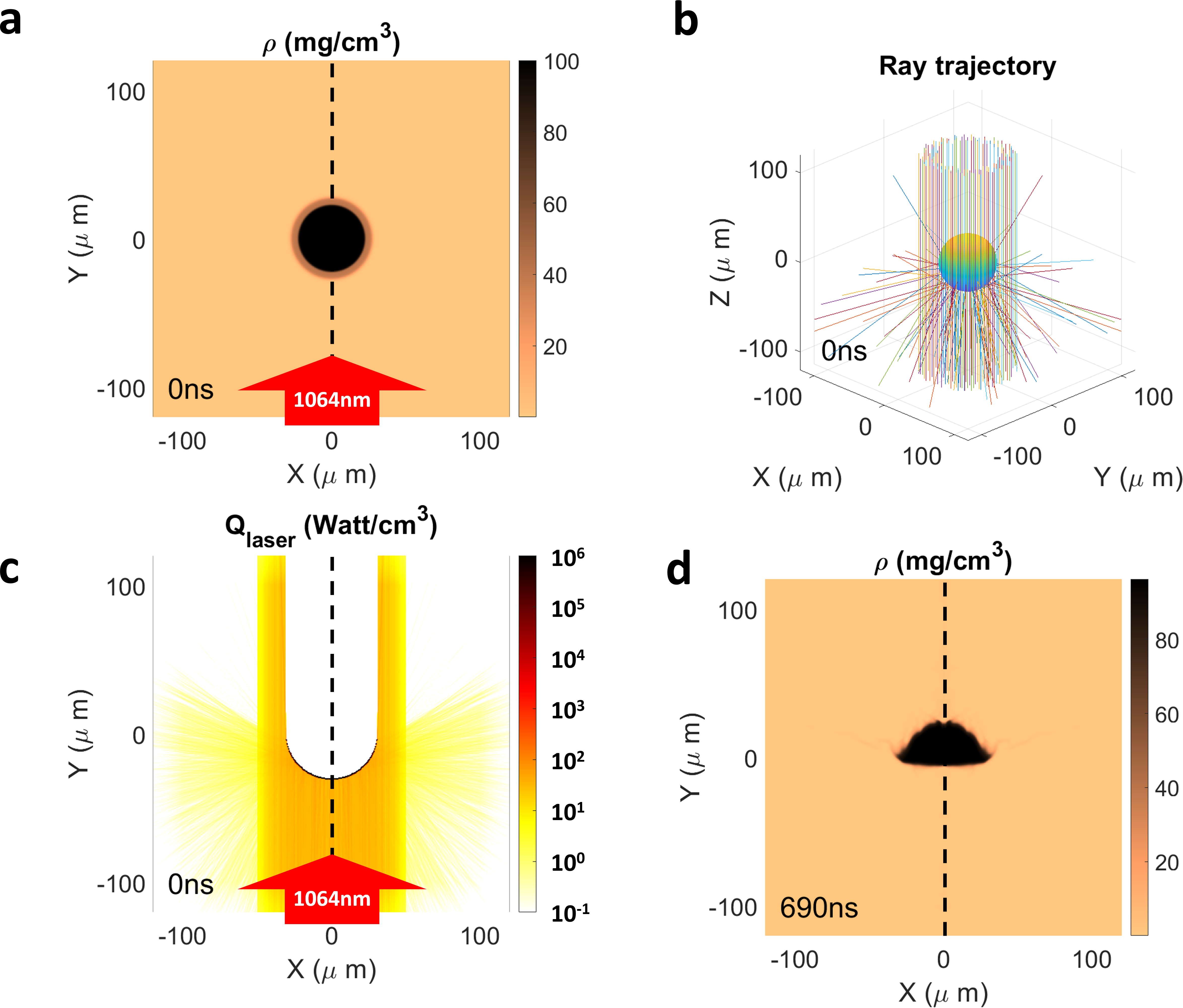
Figure 13 Laser-driven spherical water vapor target in $R-Z$ cylindrical coordinates: (a) initial density distribution, half-space mirrored; (b) 3D ray trajectories recorded in Cartesian coordinates; (c) laser volumetric heating power; (d) density distribution at $690\;\mathrm{ns}$ .

The principle of parallelizing ray tracing is to minimize the waiting time for each ray process. In cell-based algorithms (e.g., the cell-AVG method used in FLASH), the computational domain is spatially divided into many blocks (each containing multiple cells), and the smallest computational step involves a ray traversing a single block. This often leads to an inefficient situation where a few blocks have a large number of ray-tracing tasks, while most blocks have no rays at all but still need to wait due to parallel barriers. Our algorithm is slightly different: ray tracing adopts a hybrid Message Passing Interface (MPI)+OpenMP strategy. Each MPI task corresponds to one computational node (with multiple central processing unit (CPU) cores), which communicates via interlink to obtain the complete interpolated field information and is assigned a batch of rays to process. For example, if there are 4096 ray-tracing tasks, they can be distributed across eight nodes, with each MPI task processing a batch of 512 rays. Within each batch, OpenMP is used to trace each ray in parallel, achieving fine-grained task decomposition. If the communication time for the interpolated field is relatively low, the MPI+OpenMP strategy can achieve better load balancing.

MPI tasks access the full interpolation field and trace multiple rays per batch, with batch-wise depositions summed for the total energy. On an Intel Xeon 6326 CPU (2.9 GHz) with a $500\times 500$ grid and 1024 rays per batch, wall-clock times for 1, 2, 4, 8 and 16 processes are 16.106, 8.622, 4.904, 3.046 and 2.219 seconds, respectively, demonstrating near-linear speedup. Convergence studies indicate gas target simulations require at least 16,384 rays, utilizing 256 CPU cores. For 3D fluid domains, the ray count requirement exceeds ${10}^6$ rays per step.

5 Summary

This paper introduces a novel rasterization-based ray-tracing methodology that addresses key limitations of traditional cell-confined algorithms in gradient-index materials. The development of an adaptive-step integration approach eliminates the need for rays to terminate at cell interfaces, avoiding costly iterative cross-point calculations. A rasterization deposition method is introduced, decoupling the tracing algorithm from domain-specific geometries and enabling a unified, simplified computational framework for various curvilinear coordinate systems. The method’s effectiveness is demonstrated through numerical experiments, showcasing robustness, rapid convergence and accurate handling of diverse ray physics, including beam intensity and frequency shifts. Simulations of planar, cylindrical and spherical laser-ablation scenarios further indicate its enormous potential in engineering applications.

Future developments may include extending the method to more complex optical phenomena, such as non-linear laser–plasma interactions, incorporating modules for synthetic optical diagnostics and optimizing for large-scale simulations.