Dynamics-based realistic simulator for rotation rate estimation of quadcopter drones with multistatic radar

Abstract

In this paper, we introduce and validate signal processing techniques for the estimation of the individual rotation rates of multicopter’s Unmanned Aerial Vehicle (UAV), by exploiting a multistatic radar echoes. To validate the techniques, which have been introduced in our previous works, in this paper, we present a simulator for the multistatic radar echoes scattered by a UAV that integrates quadcopter’s aerodynamics with electromagnetic modeling to generate realistic radar return, characterized by blades rotating in different directions and with different rates depending on the flight trajectory to be traveled. This simulator enables the validation of signal processing.

We leverage the simulator to assess the effectiveness of autocorrelation and cross-correlation (XCF) techniques in separating multiple propellers, both in hovering and along a realistic flight trajectory. Simulated results confirm that XCF allows distinguishing counter-rotating propellers, while co-rotating ones remain unresolved due to their similar speeds. The simulator also demonstrates how variations in rotation rates can be used to infer the presence and weight of a payload. Experimental validation with a C-band continuous wave radar confirms the findings and highlights the impact of material properties on resolution. Finally, we exploit the simulator to investigate the effect of higher carrier frequencies, showing that increasing the operating frequency improves the ability to discriminate co-rotating propellers, supporting improved UAV classification, payload estimation, and trajectory prediction for anti-drone applications.

Introduction

In recent years, the extensive use of Unmanned Aerial Vehicles (UAVs) across many operational scenarios has introduced significant challenges in management and security of airspace. While drones were initially developed for military purposes, they recently found applications for various civilian applications, including environmental monitoring, search-and-rescue operations in remote or inaccessible regions, logistics, and even passenger transportation [1–3].

Effective monitoring of the air traffic in all these challenging use cases requires the development of specialized radar systems tailored for UAV monitoring. In fact, UAVs are especially elusive targets for radar. Particularly, their low-altitude, slow-speed flight patterns make these targets mostly detectable within limited ranges, where they typically compete with strong clutter returns. Moreover, their low radar cross-section (RCS), comparable to that of birds, further complicates their identification. In recent years, significant efforts have been made to characterize the RCS of commercial UAVs, with measurements conducted at frequencies ranging from 5.8 GHz to 8.2 GHz [4], 15 GHz and 25 GHz [5], and 26 to 40 GHz [6], and up to 94 GHz in [7, 8]. Recently, the RCS characterization has been leveraged in [9, 10] to improve the detection performance of UAV targets.

As UAV usage extends from military to civilian applications, distinguishing benign drone activities from potential threats becomes critical for maintaining security and ensuring effective UAV management. Several studies have explored the potential of identifying drones based on their micro-Doppler signatures, namely the distinctive features in their electromagnetic responses arising from secondary motions, such as the rotation of propellers [11–14]. Several approaches leverage propellers’ micro-Doppler signatures to distinguish UAVs from other targets [15–22]. Currently, specialized anti-drone radar systems are capable of detecting UAVs and distinguishing them from birds. This capability is also improved by the use of active electronically scanned array (AESA) radar systems, which provide multiple simultaneous antenna beams offering very long dwell times on targets of interest, with three key advantages:

1. (a) When combined with the use of continuous radar waveforms, extended time-on-target increases the signal-to-noise ratio (SNR) available at the detection stage, which is critical for detecting low RCS targets.

2. (b) Long observation times also enhance Doppler resolution, improving the radar capability to extract and analyze micro-Doppler signatures.

3. (c) In time domain, long observation times provides the possibility to observe multiple flashes from the blade tips.

Despite the advantages offered by AESA radar systems for detection, the classification of drones remains a challenging task. Addressing this issue requires ad-hoc radar processing techniques capable of extracting relevant features from UAV radar echoes.

Among these features, the rotation rates of propellers are especially interesting. Typically, UAVs are equipped with multiple propellers, each one rotating at a different speed, with values ranging between 5000 and 10.000 Rounds Per Minute (RPM) and in two possible directions: either clockwise (CW) or counter-clockwise (CCW). This is essential for stabilizing and maneuvering the drone. However, often electromagnetic models simulate the radar response backscattered by UAVs assuming uniform and constant rotation rates across for the propellers and sometimes even neglect their rotation directions.

Nevertheless, taking the differences between the propellers into proper account can be crucial to extract information from the received signals. First, detailed information about the speed and rotation direction of each propeller can be fed to a model-based classifier, enhancing our ability to distinguish between drones and birds [19, 20], or even between different UAV models. Second, even an approximate estimation of motor speeds can provide insights into the presence and weight of any payload [21, 23], which is instrumental for determining whether a drone poses a threat. Lastly, knowledge of the rotation rates and directions of each propeller can be used to predict the UAV’s trajectory based on aerodynamic principles, offering deeper insights into its behavior.

While many approached have been considered in literature, including [11–2014, 18, 24–27] for the estimation of the blade’s rotation rate, the full exploitation of bistatic and multistatic radar geometries was proposed in [28] and [29] to separate and individually estimate the rotation rates of the individual blades of a drone.

An earlier version of this paper was presented at the 21^st European Radar Conference (EuRAD 2024) and was published in its Proceedings [28]. This paper extends the findings of [28] and [29] by introducing the following innovative contributions:

1. (a) We develop a UAV radar echo simulator for multistatic radar, integrating UAV dynamics into an electromagnetic model to generate realistic radar echoes. Our simulator enables the testing of propeller rotation rate extraction techniques under diverse operational conditions, including different carrier frequencies, flight trajectories, antenna geometries, and UAV characteristics such as mass, blade length, and number of propellers. By providing a controlled and flexible platform, the simulator serves as a valuable tool for evaluating signal processing algorithms in anti-drone applications.

2. (b) We validate the autocorrelation function (ACF) and cross-correlation function (XCF) techniques presented in [28] and [29] against the simulated multistatic radar echoes at 5 receiving antennas. This includes the analysis of the capability to separately estimate the rotation rates of the four rotors of a quadcopter, with the realistic differences in rotation rate used to fly a desired trajectory following the aerodynamics laws, instead of just considering a couple of blades with arbitrarily assigned rotation rate. The usage of different frequency band is also addressed by means of the simulator.

3. (c) Moreover, we validate the ACF and XCF techniques presented in [28, 29] against multistatic experimental data. Specifically, the preliminary experimental results obtained in [28, 29] only against a couple of rotating blades are extended by using a full quadcopter UAV in hovering conditions. This analysis allows us to investigate the additional challenges introduced by the presence of four high-speed propellers, further assessing the robustness of the proposed approach.

The remainder of this paper is organized as follows. Section II presents the rotation rate estimation techniques, introduced in [28, 29] to exploit the multistatic radar configuration, while Section III describes the developed UAV multistatic radar echo simulator, detailing the assumed signal model and reference geometry. In Section IV, we leverage the simulator to analyze the capability of a C-band anti-drone radar to estimate propeller rotation rates using ACF and XCF techniques for hovering UAVs. This is followed by an experimental validation in Section V, largely extending the experimental tests conducted in [28, 29]. In Section VI, we use the simulator to study a more complex flight trajectory and evaluate the performance of ACF and XCF to estimate the individual rotation rates, also considering different carrier frequencies beyond the C-band. Finally, we draw our conclusions in Section VII.

Estimation of the propellers’ rotation rates

Several approaches can be employed to extract propeller rotation rates from radar echoes, which operate in different domains:

1. (a) Frequency domain: focus on identifying the fundamental frequency components (also known as pitch estimation techniques in the audio-signal world), by operating either on the periodogram or with spectral estimation approaches [24], such as Nonlinear Least Squares (NLS) [28, 30], Harmonic Multiple Signal Classification (Harmonic MUSIC) [31], and similar.

2. (b) Time-frequency domain: exploit the representation in the joint time-frequency plane, as short-time Fourier transform, Wavelet Transform, Wigner–Ville and similar, which can be subsequently fed into deep learning models to extract the propellers’ rotation rates [18, 25, 26].

3. (c) Time domain: a direct approach involves exploiting the peaks of ACF. In [28], a comparative analysis of time-based and frequency-based approaches, specifically ACF, NLS and HMUSIC, was conducted against both synthetic and experimental datasets, considering a single rotating propeller.

While all three methods exhibited reasonable accuracy on synthetic data – where the only disturbance was Additive White Gaussian Noise (AWGN) – the NLS approach demonstrated the highest accuracy, being the maximum likelihood estimator [28]. However, the ACF-based technique outperformed the others against experimental data, proving to be more robust against non-idealities introduced in the experiment, such as the nonlinear distortions and the presence of multipath.

Furthermore, in [28], we preliminarily introduced a new technique, operating in the Angle-Time domain, by exploiting a bistatic radar configuration, where two receiving antennas observe a single rotating propeller from two different angles. The XCF is used the temporal characteristics of the received signal to estimate the similarity of the signals received at the different antennas and therefore the periodicity of the propeller’s motion.

In this simple case, sketched in Fig. 1, angularly displaced channels observe the same signal backscattered by a propeller after a delay ${{\Delta }}T$, which depends on the propeller’s rotation rate and the angular displacement $\Delta \theta $ between the antennas. Based on this observation, we showed that the rotation rate can be estimated by measuring the delay ${{\Delta }}T$, obtained from the peak of the XCF between the two angularly displaced channels, and diving the target difference angle $\Delta \theta $ between the antennas over it. Notably, the sign of ${{\Delta }}T$ also provides information on the propeller’s rotation direction, namely it allows us to determine whether the propeller is rotating in a CW or CCW direction.

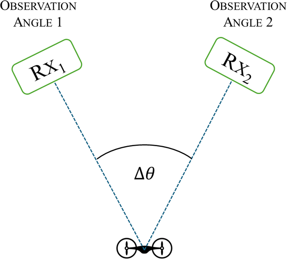
Figure 1. Multistatic radar geometry for estimation of dual propeller rotation rate and direction with two angles of view.

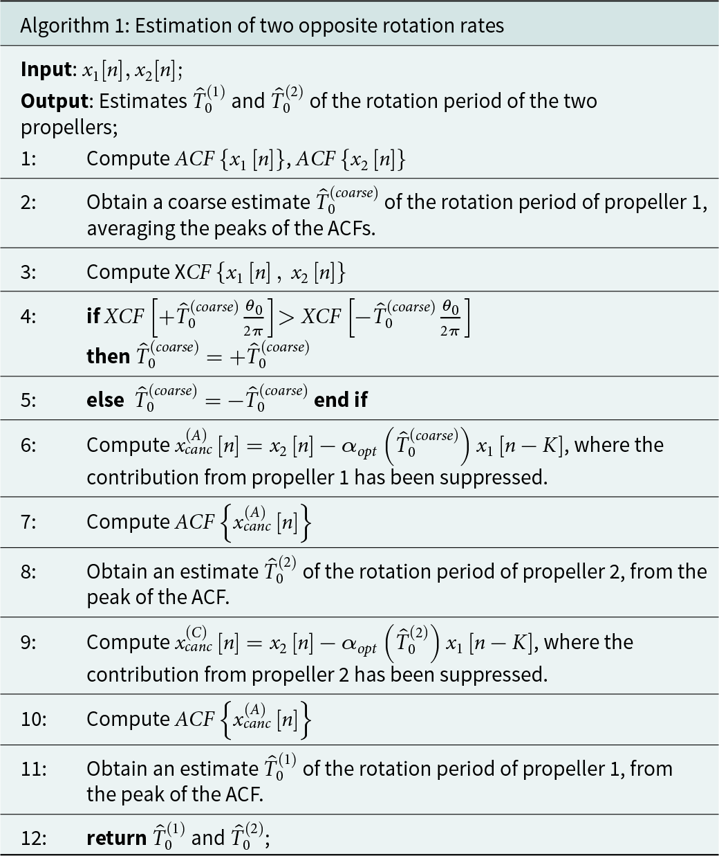
Estimating rotation rates becomes more challenging when multiple propellers are present. An initial approach to address this complexity was proposed in [29], where we exploited the XCF between multistatic radar channels to extract the rotation rates and directions of two propellers rotating in opposite directions. Assuming the two-way receiving phase centers are separated by an angle ${{\Delta }}\theta $, we observed that the contribution from a propeller rotating with period ${T_0}$ in a given direction can be suppressed by subtracting a delayed version of one received echo from the other. Specifically, denoting the signals received at observation angles 1 and 2 as ${x_1}\left[ n \right]$ and ${x_2}\left[ n \right]$, the cancelled signal ${x_{canc}}\left[ n \right]$ is obtained as follows:

(1)\begin{equation}{x_{canc}}\left[ n \right] = {x_2}\left[ n \right] - \alpha {x_1}\left[ {n - K} \right],\end{equation}

where $\alpha $ is a complex-valued coefficient and $K$ is a time shift corresponding to the time ${{\Delta }}T$ that it takes for the propeller to cover the angle ${{\Delta }}\theta $, namely $\Delta T = {T_0} \cdot \frac{{{{\Delta }}\theta }}{{2\pi }}$. The $\alpha $ value that provides the best cancellation for a given ${T_0}$, is determined by minimizing the power of the residual signal ${x_{canc}}\left[ n \right]$.

Since effectively canceling the contribution of one propeller requires knowledge of its rotation rate, Algorithm 1, proposed in proposed in [29] and reported below, first carries out a coarse estimation of the slowest rotation rate using the ACF. Then, it attempts to cancel the contribution of this propeller in both CW and CCW directions. Finally, it determines the rotation direction based on the cancelled power. Thereafter, the cancelled signal is used to estimate the rate of the opposite direction.

Notably, despite the similarity in the absolute rotation speeds in the experiment performed in [29], the XCF method effectively separated the two propellers based on their rotation directions.

Algorithm 1: Estimation of two opposite rotation rates

The reduced-scale experiments conducted in [28, 29] provided an initial experimental validation of the ACF and XCF techniques for estimating the rotation rates of UAV propellers. However, they only involved a single or a couple of counter-rotating blades and for practical limitations they used only relatively low speeds (approximately 1200 RPM), which is only one-fifth to one-tenth of the typical RPM values for UAV propellers.

To validate the techniques against more realistic conditions, next section is devoted to the definition of an echo signal generator, able to include four rotors (since the most common drones are quadcopters) with more than one propeller rotating in each direction and with the difference in the propellers rates required by the aerodynamics to fly the desired path. Later in the papers, this will be exploited to test the proposed rate estimation techniques.

Radar simulator for quadcopter UAVs

Multistatic sensor and drones’s geometry

In order to develop a realistic simulator of the radar echo backscattered by UAVs, we consider the multistatic geometry shown in Fig. 2. We define an inertial reference frame $\left\langle {X,Y,Z} \right\rangle $ ( $\mathcal{I}$ frame) centered in the transmitting antenna position and a set of $K$ receiving antennas, with coordinates defined by the position vectors ${a_k} = {\left[ {X_A^{\left( k \right)},Y_A^{\left( k \right)},Z_A^{\left( k \right)}} \right]^T},{\text{ }}k = 0, \ldots ,{\text{ }}K - 1$. Additional transmitting antennas can be added to provide a MIMO (Multiple Input Multiple Output) configuration.

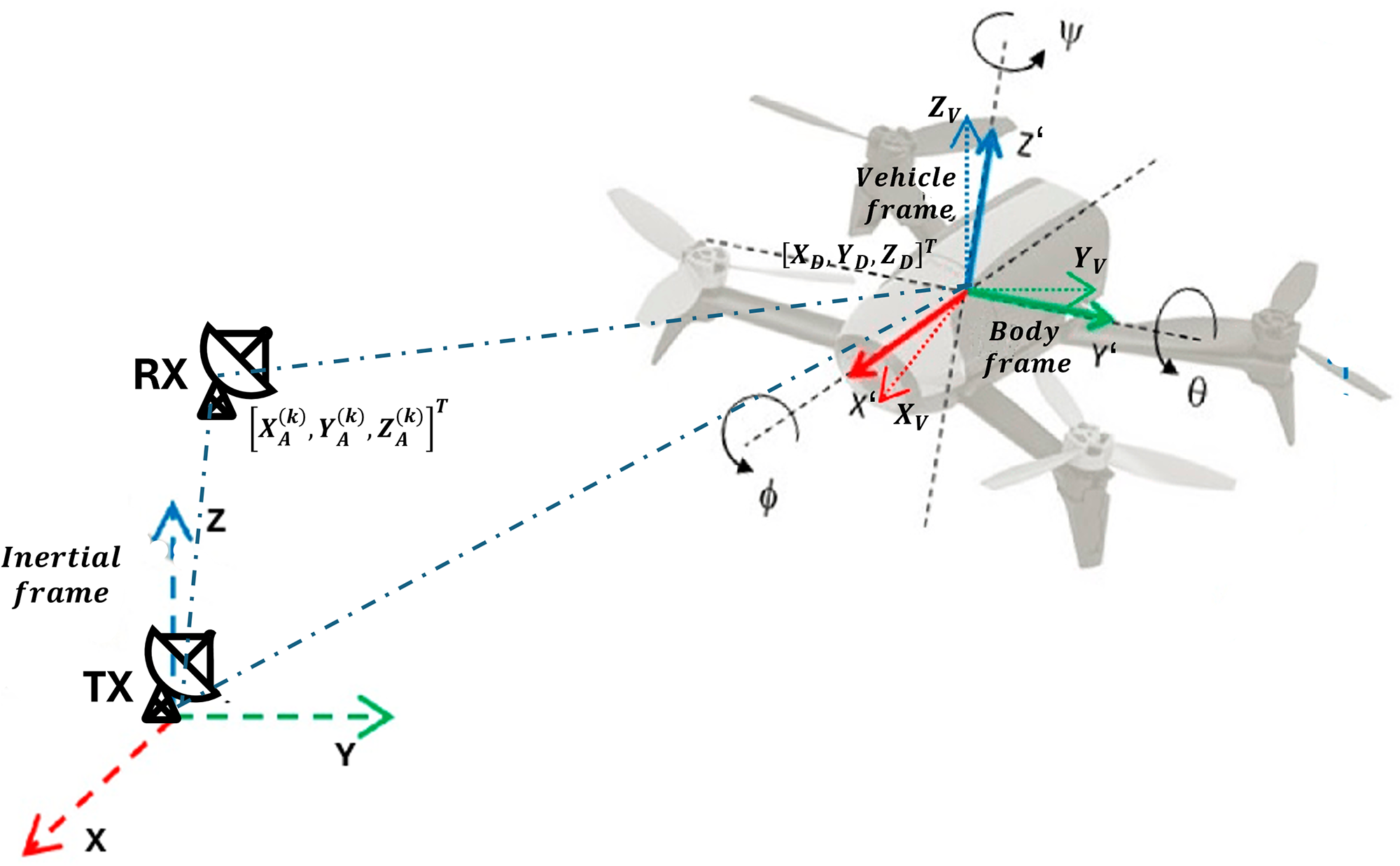
Figure 2. Three-dimensional view of the assumed system geometry, showing the reference frames considered in the model.

The position vector of the drone flown in the observed scene are denoted as $d\left( t \right) = {\left[ {{X_D}\left( t \right),{Y_D}\left( t \right),{Z_D}\left( t \right)} \right]^T}$ in the inertial frame. We let ${{\Delta }}{\theta _k},{\text{ }}k = 0, \ldots ,{\text{ }}K - 1$ denote the projections of the observation angles on the $XY$ plane for the $K$ antennas, as shown in Fig. 3. For the convenience of mathematical treatment, we define two additional reference frames:

1. (a) Vehicle reference frame $\left\langle {{X_V},{Y_V},{Z_V}} \right\rangle $ ( $\mathcal{V}$ frame), centered at the drone’s center of gravity (CG), not rotating with the drone. It provides a stable reference for describing the drone’s translational motion independently of its orientation.

2. (b) Body reference frame $\left\langle {X',Y',Z'} \right\rangle $ ( $\mathcal{B}$ frame), attached to the drone and rotating with it. It serves as a local reference system for describing the motion of individual components, such as the propellers and the blades, relative to the drone’s body.

Figure 3. Top view of the system geometry considered.

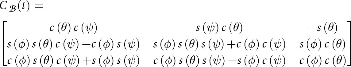
Furthermore, we let

(2)\begin{align} &{C_{|\mathcal{B}}}( t) = \nonumber \\ & {\begin{bmatrix}{c\left( \theta \right)c\left( \psi \right)} & {s\left( \psi \right)c\left( \theta \right)}& { - s\left( \theta \right)} \\ {s\left( \phi \right)s\left( \theta \right)c\left( \psi \right) {-} c\left( \phi \right)s\left( \psi \right)}& {s\left( \phi \right)s\left( \theta \right)s\left( \psi \right) {+} c\left( \phi \right)c\left( \psi \right)}& {s\left( \phi \right)c\left( \theta \right)} \\ {c\left( \phi \right)s\left( \theta \right)c\left( \psi \right) {+} s\left( \phi \right)s\left( \psi \right)} & {c\left( \phi \right)s\left( \theta \right)s\left( \psi \right) {-} s\left( \phi \right)c\left( \psi \right)} & {c\left( \phi \right)c\left( \theta \right)}\\\end{bmatrix}} \end{align}

denote the generic rotation matrix that transforms coordinates from the $\mathcal{B}$ frame to the $\mathcal{A}$ frame (where $c\left( \cdot \right)$ and $s\left( \cdot \right)$ denote the cosine and sine functions). The three reference frames considered in this paper are shown in Fig. 2, along with the Euler’s angles describing the drone’s orientation, namely roll $\phi \left( t \right)$ pitch $\theta \left( t \right)$, and yaw $\psi \left( t \right)$ rotation angles, which provide a complete description of the drone’s attitude.

To define the state of the drone, we need to define number P and positions of its propellers well as number B and angles of their blades. The $p$-th propeller is characterized by rotation rate ${\omega _p}$, and position vector $h_p^{\prime}$:

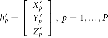(3)\begin{equation}h_p^{\prime} = \left[ {\begin{array}{*{20}{c}} {X_p^{\prime}} \\ {Y_p^{\prime}} \\ {Z_p^{\prime}} \end{array}} \right],{\text{ }}p = 1, \ldots ,P\end{equation}

in the body frame. Despite the model can accommodate any number of propellers, in any configuration, in the following, we will always assume that the UAV is equipped with $P = 4$ propellers arranged in an “X” configuration at a $45^\circ $ angle.

The instantaneous angle of the $b$-th blade in the $p$-th propeller with respect to the propeller’s hub is given by

(4)\begin{equation}{\alpha _{b,p}}\left( t \right) = {\alpha _{b,p}}\left( 0 \right) + {\omega _p}t,{\text{ }}b = 0, \ldots ,B - 1\end{equation}

where ${\alpha _{b,p}}\left( 0 \right)$ is the initial phase of the $b$-th blade in the $p$-th propeller. Finally, being ${l_B}$ the blade length, we define a blade vector $v_{b,p}^{\prime}\left( t \right)$ denoting the instantaneous position of blade tip $\left( {b,p} \right)$ in the body reference frame:

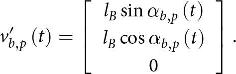(5)\begin{equation}v_{b,p}^{\prime}\left( t \right) = \left[ {\begin{array}{*{20}{c}} {{l_B}\sin {\alpha _{b,p}}\left( t \right)} \\ {{l_B}\cos {\alpha _{b,p}}\left( t \right)} \\ 0 \end{array}} \right].\end{equation}

Multistatic sensor and drones’s geometry

The block diagram of the multistatic radar echo simulator for multirotor UAV is shown in Fig. 4 and consists of two main functional blocks:

1. (a) an aerodynamic simulator, which models the dynamics of a quadcopter based on a desired trajectory, and

2. (b) a signal generator, which converts the output variables of the dynamic simulator to the inertial coordinates and evaluates the expected scattered echoes.

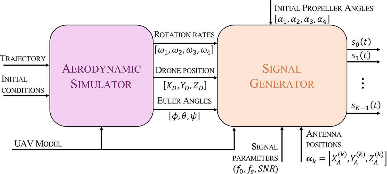
Figure 4. Block diagram of the UAV simulator driven by drone dynamics.

The signal generator outputs $K$ signals ${s_k}\left( t \right),{\text{ }}k = 0, \ldots ,K - 1,$ representing the echoes at the $K$ receiving antennas.

The aerodynamic simulator block itself consists of several functional blocks, as shown in Fig. 5:

1. (a) The position controller processes the desired trajectory input by the user, considering the drone model (including relevant parameters such as the drone’s mass ${m_D}$ and the thrust coefficient ${C_T}$), and the drone’s initial conditions. The position controller outputs attitude commands.

2. (b) The attitude controller translates the desired attitude into a feasible attitude based on the drone’s current state and parameters.

3. (c) The quadcopter control mixing translates control commands for altitude ( $Z$), roll ( $\phi $), pitch ( $\theta $), and yaw ( $\psi $) into motor throttle percentages ( ${T_1},{T_2},{T_3},{T_4})$, using a mixing matrix, ensuring accurate motor adjustments for lifting, tilting, and rotating the drone.

4. (d) Finally, the quadcopter motor dynamics converts the motor throttle percentage into real-time motor RPM, accounting for throttle cutoffs, motor behavior, and optional disturbances like wind force.

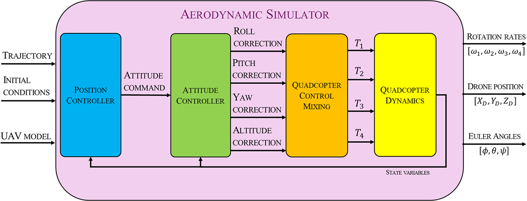
Figure 5. Block diagram of the UAV aerodynamic simulator.

At the output of the aerodynamic simulator, the state variables of the drone are available at each time instant, including position ${\left[ {{X_D}\left( t \right),{\text{ }}{Y_D}\left( t \right),{Z_D}\left( t \right)} \right]^T}$, Euler angles ${\left[ {\phi \left( t \right),{\text{ }}\theta \left( t \right),\psi \left( t \right)} \right]^T}$, as well as the instantaneous velocity and direction of the propellers, ${\omega _p},{\text{ }}p = 1, \ldots ,P$.

The signal generator block must convert the outputs of the aerodynamic simulator into the relevant geometric parameters and generate the scattered electromagnetic waveform.

The simplest way to approximate the electromagnetic response backscattered by a UAV is to exploit the so-called wire model for rotating blades, which assumes that a rotating blade exhibits the electromagnetic response of a dimensionless conductive wire [32, 33]. Although this is a highly simplified electromagnetic model that neglects several factors, such as the blade’s thickness and material composition, it is sufficient to enable preliminary considerations of practical relevance. Higher fidelity of the emulation can be obtained by accounting for the dielectric properties of the blades material and by replacing the individual wire with a cluster of wires, which fully models the shape of the blade [34–36].

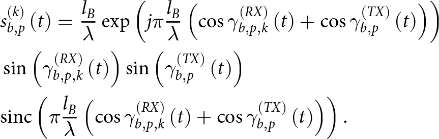
Following the derivations in [32], the wire model describes the return from the $\left( {b,p} \right)$ rotating blade can be rewritten as follows:

(6)\begin{align} & s_{b,p}^{\left( k \right)}\left( t \right) = {{{l_B}} \over \lambda }\exp \left( {j\pi {{{l_B}} \over \lambda }\left( {\cos \gamma _{b,p,k}^{\left( {RX} \right)}\left( t \right) + \cos \gamma _{b,p}^{\left( {TX} \right)}\left( t \right)} \right)} \right) \\ \nonumber & \sin \left( {\gamma _{b,p,k}^{\left( {RX} \right)}\left( t \right)} \right)\sin \left( {\gamma _{b,p}^{\left( {TX} \right)}\left( t \right)} \right) \\ \nonumber & {\rm{sinc}}\left( {\pi {{{l_B}} \over \lambda }\left( {\cos \gamma _{b,p,k}^{\left( {RX} \right)}\left( t \right) + \cos \gamma _{b,p}^{\left( {TX} \right)}\left( t \right)} \right)} \right). \end{align}

where $\lambda $ is the carrier signal wavelength, $\gamma _{b,p,k}^{\left( {RX} \right)}\left( t \right)$ is the angle between the blade vector ${v_{b,p}}\left( t \right)$ in the inertial reference frame and the Line of Sight (LoS) $r_{p,k}^{\left( {RX} \right)}\left( t \right)$ connecting the $k$-th receiving antenna to the propeller hub, and $\gamma _{b,p}^{\left( {TX} \right)}\left( t \right)$ is the angle between ${v_{b,p}}\left( t \right)$ and the LoS $r_p^{\left( {TX} \right)}\left( t \right)$ connecting the transmitting antenna to the propeller hub.

Therefore, the electromagnetic response of the UAV target including $P$ propellers, each consisting of $B$ blades, observed by the $k$-th antenna, can be modelled as the superposition of the following contributions:

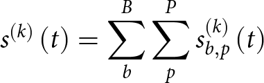(7)\begin{equation}{s^{\left( k \right)}}\left( t \right) = \mathop \sum \limits_b^B \mathop \sum \limits_p^P s_{b,p}^{\left( k \right)}\left( t \right){\text{ }}\end{equation}

where the geometric dependencies of the angles $\gamma _{b,p,k}^{\left( {RX} \right)}\left( t \right)$ and $\gamma _{b,p}^{\left( {TX} \right)}\left( t \right)$ must be appropriately obtained from the aerodynamic simulator outputs, thus taking into account the actual dynamics of the drone and providing a realistic representation of the UAV time-varying Micro-Dopplers.

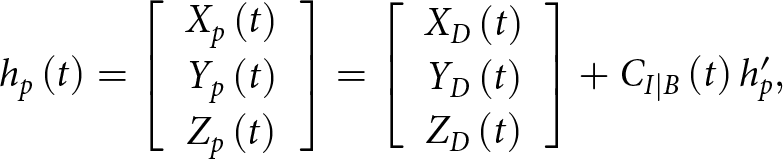
To accurately account for the UAV dynamics, we need to derive the mathematical expression for the angles $\gamma _{b,p,k}^{\left( {RX} \right)}\left( t \right)$ and $\gamma _{b,p}^{\left( {TX} \right)}\left( t \right)$ in (6), based on the system geometry described above. First, we transform the coordinates of the propeller hub from the drone body frame to the inertial frame:

(8)\begin{equation}{h_p}\left( t \right) = \left[ {\begin{array}{*{20}{c}} {{X_p}\left( t \right)} \\ {{Y_p}\left( t \right)} \\ {{Z_p}\left( t \right)} \end{array}} \right] = \left[ {\begin{array}{*{20}{c}} {{X_D}\left( t \right)} \\ {{Y_D}\left( t \right)} \\ {{Z_D}\left( t \right)} \end{array}} \right] + {C_{I|B}}\left(t \right)h_p^{\prime},\end{equation}

where ${C_{\mathcal{I}|\mathcal{B}}}\left( t \right)$ is the rotation matrix that transforms coordinates from the drone body frame to the inertial frame. Then, we define the LoS vector

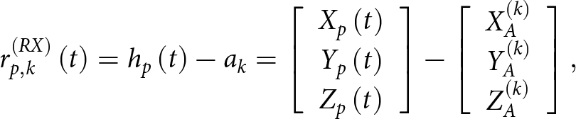(9)\begin{equation}r_{p,k}^{\left( {RX} \right)}\left( t \right) = {h_p}\left( t \right) - {a_k} = \left[ {\begin{array}{*{20}{c}} {{X_p}\left( t \right)} \\ {{Y_p}\left( t \right)} \\ {{Z_p}\left( t \right)} \end{array}} \right] - \left[ {\begin{array}{*{20}{c}} {X_A^{\left( k \right)}} \\ {Y_A^{\left( k \right)}} \\ {Z_A^{\left( k \right)}} \end{array}} \right],\end{equation}

connecting the $k$-th receiving antenna to the $p$-th propeller’s hub in the inertial frame. Similarly, for the transmitting antenna, we have the LoS vector

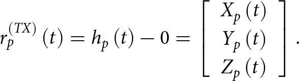(10)\begin{equation}r_p^{\left( {TX} \right)}\left( t \right) = {h_p}\left( t \right) - 0 = \left[ {\begin{array}{*{20}{c}} {{X_p}\left( t \right)} \\ {{Y_p}\left( t \right)} \\ {{Z_p}\left( t \right)} \end{array}} \right].\end{equation}

Finally, by deriving the propeller blade vector describing the position of the blade tip in the inertial frame

(11)\begin{equation}{v_{b,p}}\left( t \right) = {C_{I|B}}\left( t \right)v_{b,p}^{\prime}\left( t \right),\end{equation}

we can write the angles $\gamma _{b,p}^{\left( {TX} \right)}\left( t \right)$ and $\gamma _{b,p,k}^{\left( {RX} \right)}\left( t \right)$ as

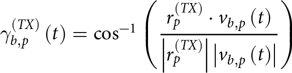(12)\begin{equation}\gamma _{b,p}^{\left( {TX} \right)}\left( t \right) = {\text{co}}{{\text{s}}^{ - 1}}\left( {\frac{{r_p^{\left( {TX} \right)} \cdot {v_{b,p}}\left( t \right)}}{{\left| {r_p^{\left( {TX} \right)}} \right|\left| {{v_{b,p}}\left( t \right)} \right|}}} \right)\end{equation}

for the transmitting antenna and

(13)\begin{equation}\gamma _{b,p,k}^{\left( {RX} \right)}\left( t \right) = {\text{co}}{{\text{s}}^{ - 1}}\left( {\frac{{r_{p,k}^{\left( {RX} \right)}(t) \cdot {v_{b,p}}\left( t \right)}}{{\left| {r_{p,k}^{\left( {RX} \right)}(t)} \right|\left| {{v_{b,p}}\left( t \right)} \right|}}} \right)\end{equation}

for the $K$ receiving antennas. Here, $ \cdot $ denotes the dot product and $\left| \cdot \right|$ denotes the vector norm.

We notice that a similar attempt is synthetically reported in [37]; however, our simulator enables a realistic simulation driven by the drone dynamics, which allowed us to study a variety of complex operational scenarios. In particular, our simulator allows the generation of scattered waveforms accounting for the implications of the basic aerodynamic principles:

1. (a) Half of the propellers rotate CW, while the other half rotates CCW; otherwise, the UAV would rotate uncontrollably about its center of mass.

2. (b) When the UAV is not in hovering mode, the rotational speeds of the propellers differ to enable maneuvering operations, with typical differences ranging from 1% to 15%, depending on the drone’s size, type, and the abruptness of the maneuver.

For this reasons the developed simulator also provides a platform for testing the estimation techniques for the propeller rotation rates, which can be applied to real-world data, possibly allowing the radar to determine the presence and weight of any payload, to classify between different UAV models, and to predict the drone’s trajectory.

Rotation rate estimation in hovering conditions

The analysis presented in this section is based on the realistic simulator introduced in Section III and aims at assessing the scalability of the ACF and XCF techniques in Section II to more realistic multistatic radar echo signals, specifically considering higher RPM values and multiple CW and CCW propellers. Moreover, we aim at assessing the estimation potentialities provided by the exploitation of multistatic radar with a higher number of receiving antennas.

For our analysis, we consider the multistatic antenna geometry depicted in Fig. 6, with K = 5 receiving antennas at a distance $50{\text{ }}m$ from the UAV position, uniformly distributed on a circular arc covering an angular sector of $90^\circ $, with an angular separation of ${{\Delta }}{\theta _k} = 22.5^\circ $ between adjacent elements. The transmitting antenna is located just above the central receiving antenna (RX3). A quadcopter UAV is considered, with an unloaded mass of ${m_{UAV}} = 1023{\text{ }}g$, equipped with $P = 4$ propellers, each including $B = 2$ blades of length ${l_B} = 13{\text{ }}cm$.

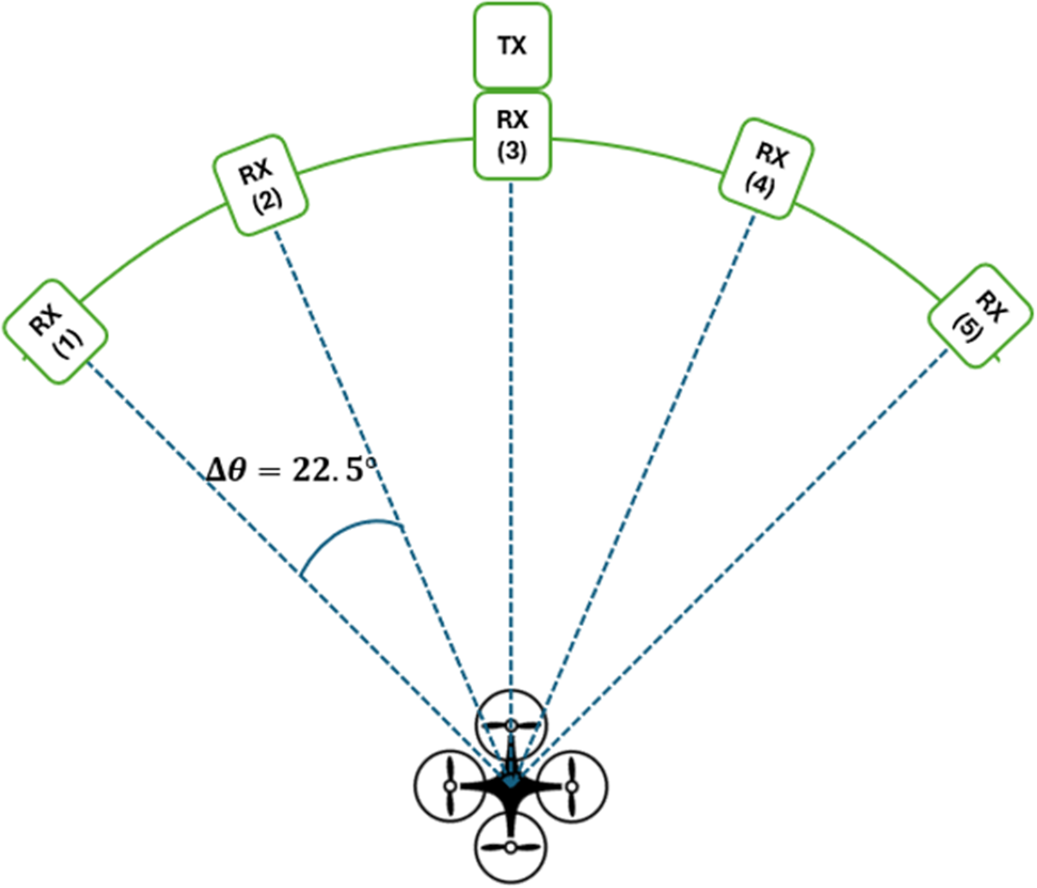
Figure 6. Top view of the antenna positions assumed in the simulation.

To replicate the operating conditions of the experiments conducted in [28, 29] with reference to a C-Band anti-drone radar, a single tone waveform is emitted at ${f_c} = 5.5{\text{ }}GHz$. and a sampling frequency of ${f_s} = 1{\text{ }}MHz$ is assumed at the receivers. The dynamic simulator activated to maintain the drone in hovering at the center of the circular arc described by the receiving antennas. Under this condition, the propellers are all assigned the same rotation rate of ${\omega _p} = 4108$ RPM, while the initial phases are assumed to be randomly assigned.

Figure 7 shows a selected portion of the generated signal (black curve) for one of the receiving antennas (total length ${T_{sim}} = 30s$) between 7.003 ms and 7.0249 ms, with colored arrows indicating the flashes of the four propellers. Similarly, the red curve represents the received with a synthetic AWGN with an SNR of 10 dB.

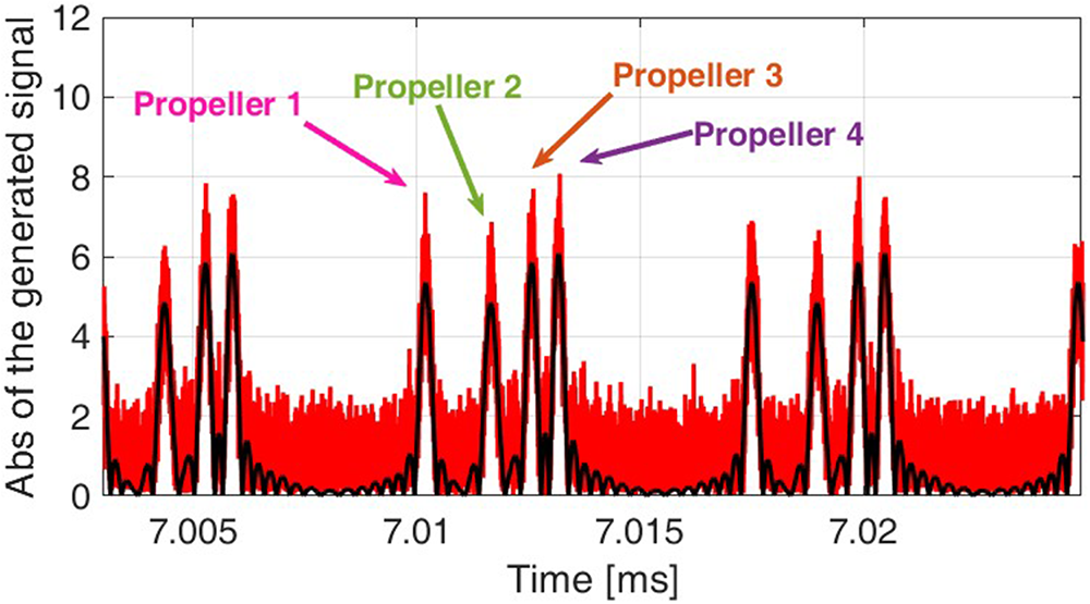
Figure 7. Signal received at the $k$-th antenna, showing the return of the four propellers. The arrows denote the rotation period of the propellers.

We notice that in Fig. 7, separate blade flashes for the four motors are clearly distinguishable. However, depending on the SNR, the relative positions of the antennas and the initial angle of the blades, one or more flashes might overlap in time and add either constructively or destructively Therefore, a simple visual inspection of the time-domain signal is generally not sufficient to estimate the rotation rates.

Rotation rate estimation for hovering UAVs using ACF

To validate the ACF technique proposed in [28] using the developed simulator, we employ a batch processing strategy. Specifically, the signal at the $k$-th antenna is divided into batches of duration ${T_{batch}}$. The ACF of each batch is evaluated, and the peak closest to the zero-lag peak is extracted to estimate the signal’s periodicity within the batch at hand. To set the batch duration, we must ensure that it satisfies two conditions: ${T_{batch}}$ must be greater than the signal’s period, and it must also be short enough to guarantee that the propeller’s rotational speed remains approximately constant within the batch. Since the UAV is in hovering conditions and all four propellers rotate at the same speed, a periodic component with period ${T_0}/B$ should be observed, where $B$ is the number of blades in each propeller and ${T_0} = 60/{\omega _p}$ is the period of the individual propeller.

The ACF of a specific signal batch of duration ${T_{batch}} = 100{\text{ }}ms$ received by a single antenna is shown in Fig. 8, showing a period of, consistent with a rotation period ${T_0} \approx 14.6{\text{ }}ms$. In practice, during the selected batch, depending on initial conditions and numerical roundings, the simulator imposes the following rotation rates to the four propellers to keep the hovering condition: ${\omega _1} = - 4110{\text{ }}RPM$, ${\omega _1} = + 4115{\text{ }}RPM$, ${\omega _1} = - 4121{\text{ }}RPM$, ${\omega _1} = +\,4111{\text{ }}RPM$ (opposite signs denote opposite rotation directions), corresponding to a rotation period ${T_0} \approx 14.6{\text{ }}ms$.

Figure 8. Autocorrelation function of the signal backscattered by the $P$ propellers for the hovering UAV, measured within a batch of duration ${T_{batch}} = 100{\text{ }}ms$.

The following observations are in order:

1. (a) The ACF shows the correct peaks spaced by ${T_0}/2$, corresponding, thus showing to be effective at the realistic motor speeds, more than five times higher than in [28].

2. (b) Since the rotation rates of the four propellers are almost identical in hovering conditions, there is no way to determine how many propellers are present in the UAV.

3. (c) Additional spurious peaks are visible in the ACF, due to the combination of the signals from different propellers. These are expected to be reduced by averaging the ACFs from the $K$ antennas.

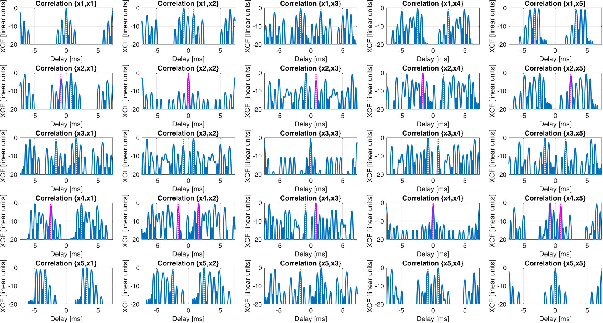
Figure 9. Matrix of all the possible auto/cross-correlations with $K = 5$ antennas for an unloaded UAV in hovering.

Overall, the results confirm the validity of the findings in [28], demonstrating the practical utility of the ACF-based technique for estimating the rotation rates of UAV propellers.

Rotation rate estimation for hovering UAVs using XCF

Having in mind the idea to exploit the XCF among the signals received at the different antennas, Fig. 9 shows the 5 × 5 matrix of all the auto/cross-correlations, obtained using the $K = 5$. The following observations are in order:

1. (a) Based on the discussion in Section II, we expect to find XCF peaks at the time delay ${{\Delta }}T$, required by the blade to rotate, so that the second antenna sees it from the same angle of the first antenna at time 0. This obviously depends on the angular separation ${{\Delta }}\theta $ (known) and on the rotation period ${T_0}$ of the propeller:

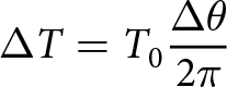(14)\begin{equation}\Delta T = {T_0}\frac{{\Delta \theta }}{{2\pi }}\end{equation}

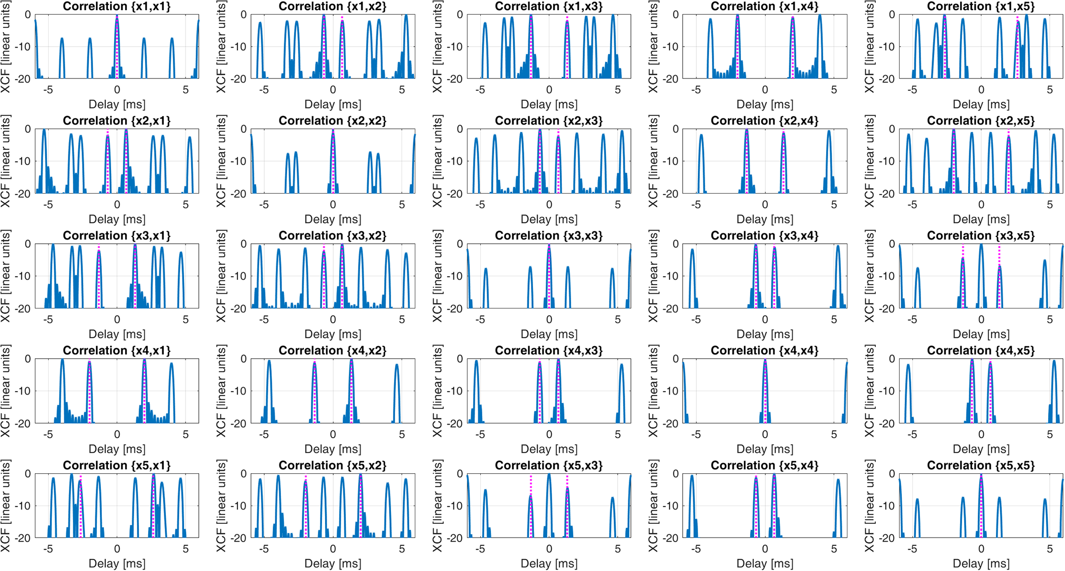
Figure 10. Matrix of all the possible auto/cross-correlations with $K = 5$ antennas for a loaded UAV in hovering.

The magenta lines in Fig. 9 indicate the theoretical values based on (14) that clearly appear in the correct positions.

1. (b) It is apparent that by measuring the time lag of this peak and scaling it by the angular separation $\Delta \theta $ between the two antennas, the propeller’s rotation period can be correctly estimated

2. (c) Unlike using the ACF, using the XCF propellers rotating CW and CCW can be distinguished based on the sign of the time lag of the main XCF peaks, as demonstrated in [29] for bicopters. Particularly, in the considered scenario, the estimated rotation rate for the CW propellers is $ + 4108{\text{ }}RPM$, while the one for CCW propellers is $ - 4108{\text{ }}RPM$.

3. (d) In the hovering case, co-rotating propellers cannot be distinguished, since they have identical rotation rates, aside from minor fluctuations used to stabilize the drone against external disturbances like wind force.

4. (e) Also the XCFs exhibits several spurious peaks in addition to the main ones. These spurious peaks are due to the angles assumed by the individual blades with respect to the antennas, which causes periodic components in the signal, unrelated to the propellers’ rotation rates. Averaging over multiple observation angles could be exploited to reduce these peaks.

The analysis above clearly confirms the results in [29], that XCF between angularly separated channels is not just an alternative to ACF but is essential for separating contributions from propellers rotating in opposite directions.

While we are unable to distinguish between the two co-rotating propellers in hovering conditions, this is not a major issue until the drone remains stationary, since it does not pose a potential threat. Indeed, by exploiting the cancellation, we can separate the two co-rotating propellers at least when the drone is in motion, we could still determine the overall number of propellers, classify the UAV, infer its movement, and predict its potential trajectory as soon as the UAV begins to maneuver. In addition, being able to estimate the average rotation rate of each pair of co-rotating propellers could already prove useful. For instance, if the drone is equipped with a payload, the propellers must rotate faster to provide the thrust needed to counterbalance the additional weight. Therefore, estimating the average rotation rates of each pair of co-rotating propellers could provide an indication of the carried weight, providing valuable information for determining the UAV’s operational characteristics and its potential threat level. For instance, a sudden decrease in the propellers rotation rates might suggest the in-flight release of a payload.

In order to show this, we repeat the previous analysis under the same operational conditions, only increasing the drone’s mass to ${m_{tot}} = {m_{UAV}} + {m_{payload}} = 1523{\text{ }}g$ to simulate a payload with mass ${m_{payload}} = 500{\text{ }}g$. We note that in the conducted simulation, the payload is assumed to be positioned near the drone’s center of gravity, such that any increase in the moments of inertia compared to the unloaded condition are kept relatively small.

The 5 × 5 matrix of correlation signals obtained in this case is shown in Fig. 10. The following observations are in order:

1. (a) As in the previous case study, co-rotating propellers are indistinguishable, since they have identical rotation rates.

2. (b) Propellers with opposite rotation directions are still easily separable.

3. (c) When a $500{\text{ }}g$ payload is added to the drone, the propellers’ rotation rates in hovering conditions increase, resulting in an estimated rotation rate of, compared to the $ \pm 4108{\text{ }}RPM$ estimated in unloaded case.

4. (d) Although it is not possible to directly distinguish the contributions of co-rotating propellers, the variation in the rotation rates allows inferring the presence or absence of a payload and estimating its weight. Specifically, the total mass of a quadcopter in hovering is related to the rotational speed of the propellers through the following equation:

(15)\begin{equation}{m_{tot}} = {m_{UAV}} + {m_{payload}} = \frac{{4{c_T}{\omega ^2}}}{g},\end{equation}

where ${c_T}$ is the thrust coefficient of a single propeller, independent of the payload mass, and $g$ is the gravitational acceleration. Therefore, the ratio between the total mass with payload and the mass of the unloaded UAV can be expressed as a function of the ratio between the hovering rotation rates with and without the payload, respectively denoted as ${\omega _{UAV + payload}}$ and ${\omega _{UAV}}$

(16)\begin{equation}\frac{{{m_{tot}}}}{{{m_{UAV}}}} = \frac{{\omega _{UAV + payload}^2}}{{\omega _{UAV}^2}}.\end{equation}

By knowing the unloaded mass of the quadcopter and measuring the change in rotational speed during hovering, the weight of the carried payload can be estimated.

Experimental results in hovering conditions

After testing the techniques introduced in [28, 29] against simulated UAV radar echoes in hovering conditions, we now validate these results against experimental data.

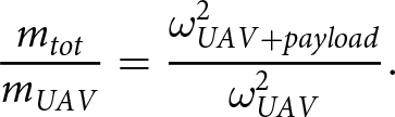
The experimental setup is shown in Fig. 11. Specifically, we consider a multistatic radar deployed in an indoor environment, including six Ubiquiti Networks UMA-D antennas designed for Wi-Fi applications. As in the simulation, the transmitting antenna emitted a continuous-wave sinusoidal tone at ${f_c} = 5.5{\text{ }}GHz$, while the 5 receiving antennas were uniformly spaced within a 90° angular sector. All antennas operated with horizontal polarization. A DJI Mavic Pro UAV equipped with four propellers, each consisting of two plastic blades, was positioned at the center of the antennas, hovering at $R = 1.3{\text{ }}m$ from the antennas and at the same height as the receivers, $H = 1.5{\text{ }}m$. The transmitting antenna was placed directly above the central receiving antenna for symmetry.

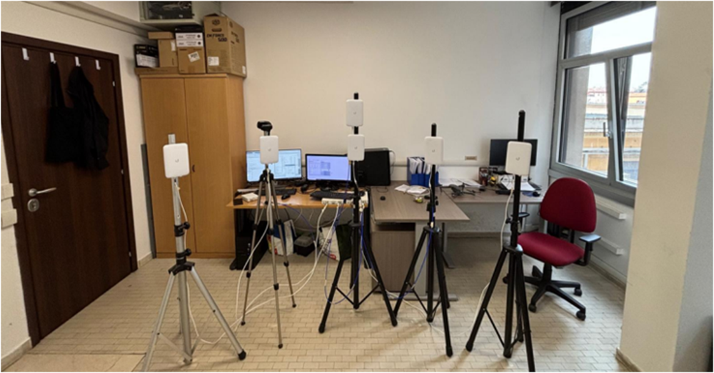
Figure 11. Experimental setup.

The transmitter was connected to an Ettus USRP-B210 board, responsible for generating and transmitting the sinusoidal waveform. The five receiving antennas were connected to two National Instruments USRP-2955 boards. To mitigate potential carrier frequency offsets caused by mismatches in the local oscillators of the three boards, a reference copy of the transmitted signal was split and fed to the receiving boards. A top view of the TX/RX hardware is shown in Fig. 12.

Figure 12. TX/RX hardware configuration.

Figure 13 shows the correlation signals computed for all channel pairs over a $100{\text{ }}ms$ signal batch, after a preliminary clutter suppression stage that removed stationary reflections from the room and UAV body. The magenta vertical lines indicate the expected peak positions, corresponding to a rotational speed of $5850{\text{ }}RPM$, as obtained from the UAV’s controller.

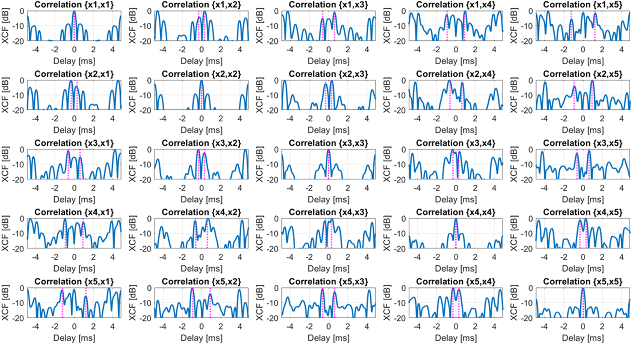
Figure 13. Matrix of all the possible auto/cross-correlations with $K = 5$ antennas using real data for an UAV in hovering conditions.

The experimental results confirm the observations made in simulation. Specifically, the time lags of the XCF peaks allow us to distinguish the counter-rotating propellers, as their respective peaks are clearly separated. In the experiment, the rotation speeds are subject to minor fluctuations required to stabilize the hovering drone. While these fluctuations could, in principle, help distinguish between the two pairs of co-rotating propellers, they remain too small for effective separation, so that the resulting peaks appear overlapped as in the simulation.

Moreover, multiple spurious peaks appear that could be reduced by averaging across different correlation functions, improving the estimation accuracy.

Finally, compared to the simulation, the ACF/XCF peaks in Fig. 13 appear wider. This is likely due to the material of the propellers, which do not behave as perfectly conductive wires as assumed in our model, resulting in a wider mainlobe. This effect is particularly significant, as the degraded peak resolution makes it more challenging to separate co-rotating propellers when they rotate at similar speeds.

Rotation rate estimation for realistic flight conditions

In this section, we extend the analysis to UAVs in motion, following a predefined trajectory. In this scenario, all four propellers generally rotate at different speeds. We investigate whether, under these practical operating conditions, the ACF and XCF techniques can effectively distinguish each pair of co-rotating propellers.

We consider the same geometry illustrated in Fig. 6. The same quadcopter UAV is used for this simulation starting from the hoovering condition of Section IV. In this scenario, the UAV follows the complex trajectory shown in Fig. 14 over a total simulation time of ${T_{sim}} = 30s$.

Figure 14. “RADAR” trajectory followed by the drone in the simulation.

Since the propellers’ rotation rates vary during flight, in principle it should now be possible to distinguish between the two CW and two CCW propellers using ACF and XCF techniques. Specifically, Fig. 15 shows the evolution of the four rotational speeds ${\omega _p}$ over time as the drone follows the desired trajectory.

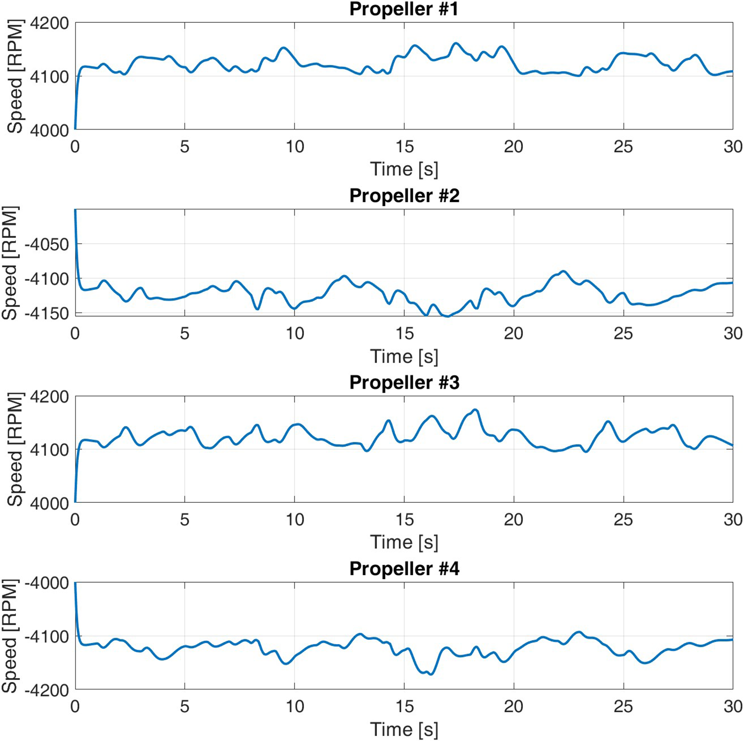
Figure 15. Rotational speed ${\omega _p}$ of the $P$ propellers as a function of time for the “RADAR” trajectory, in RPM units. Positive sign denotes a clockwise rotation.

By processing the received signals in batches of duration ${T_{batch}} = 100{\text{ }}ms$, we obtain the 5 × 5 matrix of auto/cross correlation signals shown in Fig. 18. The following observations are in order:

1. (a) As in the hovering case, counter-rotating propellers can be separated based on the sign of the time lags of the corresponding XCF peaks.

2. (b) Unfortunately, despite the variations in the rotation rates, co-rotating propeller remain too similar, causing their peaks in the XCF to overlap.

3. (c) The simulator indicates that the maximum speed difference between co-rotating propellers is at most 60 RPM, which appears insufficient for clear separation at this carrier frequency.

4. (d) Notably, distinguishing co-rotating propellers is inherently more challenging in XCF than in ACF, as XCF estimates a fraction of the rotation period rather than the full period, leading to closer peak positions.

These results confirm that a continuous wave radar operating in the C-band at ${f_c} = 5.5{\text{ }}GHz$ cannot effectively discriminate co-rotating propellers in realistic flight conditions. To overcome this limitation, alternative approaches can be explored at both the signal processing and system design levels. At the processing level, advanced techniques could be developed to extract the rotation rates, possibly by jointly analyzing all the correlation functions in Fig. 16 to enhance resolution. At the system design level, increasing the carrier frequency of the transmitted waveform could improve separation between similar rotation rates. Specifically, according to the wire model in (6), a rotating propeller behaves like an antenna with a sinc-like response, where the beamwidth depends on the ratio between the blade length ${l_b}$ and the signal wavelength $\lambda $. Therefore, a radar system operating at higher frequencies could achieve sharper ACF/XCF peaks, potentially enabling discrimination of all four propellers.

In first approximation, it can be stated that the width of the ACF and XCF peaks is equal to the width of the echo. Therefore, the condition to be satisfied to allow the separation of the peaks can be expressed as follows:

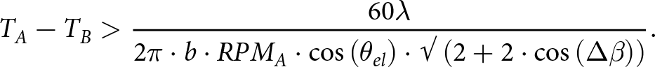(17)\begin{equation}{T_A} - {T_B} \gt \frac{{60\lambda }}{{2\pi \cdot b \cdot RP{M_A} \cdot \cos \left( {{\theta _{el}}} \right) \cdot \surd \left( {2 + 2 \cdot \cos \left( {\Delta \beta } \right)} \right)}}.\end{equation}

where

1. (a) ${T_A}{\text{ }}e{\text{ }}{T_B}$ are the rotation periods of the first and second propellers, respectively ( ${T_A} \gt {T_B}$),

2. (b) ${{\Delta }}\beta $ is the bistatic angle relative to the considered receiving antenna, expressed in radians,

3. (c) $RP{M_A}$ is the rotation speed of the slower propeller, expressed in rotation per minute.

The difference between the rotation periods of the two propellers, ${T_A} - {T_B}$, can be rewritten as a function of $RPM$:

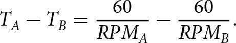(18)\begin{equation}{T_A} - {T_B} = \frac{{60}}{{RP{M_A}}} - \frac{{60}}{{RP{M_B}}}.\end{equation}

Therefore, to separate a pair of peaks corresponding to rotors rotating at different speeds $RP{M_A}$ e $RP{M_B}$, it is required that:

(19)\begin{equation}\left( {1 - \frac{{RP{M_A}}}{{RP{M_B}}}} \right) \cdot \frac{{{l_b}}}{\lambda } \cdot \cos \left( {{\theta _{el}}} \right) \cdot \surd (2 + 2 \cdot \cos \left( {{{\Delta }}\beta } \right) \gt 1\end{equation}

Namely the relative variation of the angular rotation speed $\frac{{\Delta RPM}}{{RP{M_B}}}$ must be larger than the flash angular aperture normalized to quantities depending of the elevation angle and antenna separation

(20)\begin{equation}\frac{{\Delta RPM}}{{RP{M_B}}} \gt \frac{{\lambda /{l_B}}}{{\cos \left( {{\theta _{el}}} \right) \cdot \surd (2 + 2 \cdot \cos \left( {\Delta \beta } \right)}}.\end{equation}

This equation can also be used to size the system. It is apparent that for assigned ${{\Delta }}RPM = {\text{ }}RP{M_B} - RP{M_A}$and blade length, a higher separation capability is provided by operating at higher frequencies (namely, with smaller $\lambda $ values).

The simulator introduced in Section III provides a powerful tool for evaluating these scenarios, allowing us to systematically test the impact of different carrier frequencies on rotation rate estimation. Specifically, we repeat simulations for a drone following the trajectory in Fig. 14 with carrier frequencies of $36{\text{ }}GHz$ and $98{\text{ }}GHz$. Figure 17 compares the ACFs of a $100{\text{ }}ms$ signal batch at the different frequencies considered. To obtain these curves, the ACFs from the signals at the $K = 5$ antennas were averaged to mitigate the effect of spurious peaks. For example, the blue curve at $5.5{\text{ }}GHz$ represents the average of the curves shown along the main diagonal of the 5 × 5 matrix of correlation signals in Fig. 16. Figure 18 provides an enlarged view of Fig. 17 around the average propellers’ period ${T_0}$. As apparent, the lower level of the ACF at the highest frequencies is introduced to visually express the higher attenuation affecting the echoes at the higher frequencies, which is clearly dependent on the target range, as encoded by the radar equation.

From these two figures, it is clear that the ability to resolve propellers rotating at very similar speeds improves as the carrier frequency increases. Specifically, at $36{\text{ }}GHz$, three of the four propellers can be distinguished, while at $98{\text{ }}GHz$, all four propellers can be identified. Of course, $98{\text{ }}GHz$ is a very high frequency and is not intended for long-range surveillance applications. Therefore, although increasing the frequency from the C-band up to W-band clearly improves the capability of distinguishing between similar rotation rates, intermediate values of frequency could still be effective, when supported with processing techniques able to fully exploit the multistatic geometry so that to choose the XCF between the couples of antennas that allow the highest separation among the blade flashes. Since the best selection depends on the initial blade angles, this needs to be adaptively selected for each processing batch.

Figure 16. Matrix of all the possible auto/cross-correlations with $K = 5$ antennas in case study B-UAV following the “RADAR” trajectory.

Figure 17. ACF of a signal batch for different carrier frequencies. Higher values of frequency result in narrower ACF peaks.

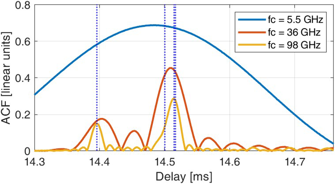
Figure 18. ACF of a signal batch for different carrier frequencies. The zoom around the average propellers’ period reveals that the four rotation rates can be effectively separated at ${f_c} = 98{\text{ }}GHz$.

Conclusions

In this paper, we addressed the estimation of propeller rotation rates from UAV radar echoes in a multistatic radar configuration. Knowledge of the propellers’ rotation rates can potentially allow the radar to determine the presence and weight of any payload, classify different UAV models, and predict the drone’s trajectory.

To study the extraction of rotation rates, we first developed a simulator that integrates UAV dynamics with an electromagnetic model, providing an accurate representation of UAV radar echoes in realistic flight conditions. The developed simulator allowed us to test the ACF and XCF techniques previously introduced in [28, 29], and to study the impact of multiple propellers rotating at realistic speeds. Moreover, we further validated the ACF and XCF techniques on experimental data for a hovering drone, extending the preliminary tests in [28, 29]. The results confirmed the findings from our simulation.

Overall, the study demonstrated the ability to discriminate counter-rotating propellers using ACF and XCF, but highlighted the challenges in distinguishing co-rotating ones, particularly at lower frequencies. These findings highlight the need for combining the use of higher carrier frequencies – beyond the C band – with advanced signal processing techniques to extract all rotation rates effectively.

Future work will focus on addressing these limitations by developing more advanced signal processing techniques that fully exploit rich multistatic radar geometries, building on the tests enabled by the simulator presented in this paper.