


1. Introduction
For an integer $k\geq 2$
, the k-core of a graph G is the largest induced subgraph of G with minimum degree at least k. It was first introduced in [Reference Bollobás, Bollobás and Press5] to find large k-connected subgraphs, and since then several studies have been devoted to investigating the existence and the order of the k-core. Apart from theoretical interest, the k-core has been applied to the study of social networks [Reference Bhawalkar, Kleinberg, Lewi, Roughgarden and Sharma4, Reference Huang, Cheng, Qin, Tian and Yu19], graph visualizing [Reference Alvarez-Hamelin, Dall’Asta, Barrat and Vespignani1, Reference Carmi, Havlin, Kirkpatrick, Shavitt and Shir13], and biology [Reference You, Lei, Zhu, Xia and Wang32]. See also [Reference Kong, Shi, Wu and Zhang24] for an extensive discussion on its applications. The seminal paper [Reference Pittel, Spencer and Wormald30] determined the threshold for the appearance of a non-empty k-core in binomial random graphs and uniform random graphs. The order of the k-core has been studied in different random graph ensembles such as binomial random graphs [Reference Łuczak28], uniformly chosen random graphs and hypergraphs with specified degree sequence [Reference Cooper17, Reference Fernholz and Ramachandran18, Reference Janson and Luczak21, Reference Janson and Luczak22, Reference Molloy29], the Poisson cloning model [Reference Kim23], and the pairing-allocation model [Reference Cain and Wormald12]. While almost all the previous work focused on the k-core of homogeneous random graphs, [Reference Riordan31] determined the asymptotic order of the k-core for a large class of inhomogeneous random graphs introduced in [Reference Bollobás, Janson and Riordan7].
$k\geq 2$
, the k-core of a graph G is the largest induced subgraph of G with minimum degree at least k. It was first introduced in [Reference Bollobás, Bollobás and Press5] to find large k-connected subgraphs, and since then several studies have been devoted to investigating the existence and the order of the k-core. Apart from theoretical interest, the k-core has been applied to the study of social networks [Reference Bhawalkar, Kleinberg, Lewi, Roughgarden and Sharma4, Reference Huang, Cheng, Qin, Tian and Yu19], graph visualizing [Reference Alvarez-Hamelin, Dall’Asta, Barrat and Vespignani1, Reference Carmi, Havlin, Kirkpatrick, Shavitt and Shir13], and biology [Reference You, Lei, Zhu, Xia and Wang32]. See also [Reference Kong, Shi, Wu and Zhang24] for an extensive discussion on its applications. The seminal paper [Reference Pittel, Spencer and Wormald30] determined the threshold for the appearance of a non-empty k-core in binomial random graphs and uniform random graphs. The order of the k-core has been studied in different random graph ensembles such as binomial random graphs [Reference Łuczak28], uniformly chosen random graphs and hypergraphs with specified degree sequence [Reference Cooper17, Reference Fernholz and Ramachandran18, Reference Janson and Luczak21, Reference Janson and Luczak22, Reference Molloy29], the Poisson cloning model [Reference Kim23], and the pairing-allocation model [Reference Cain and Wormald12]. While almost all the previous work focused on the k-core of homogeneous random graphs, [Reference Riordan31] determined the asymptotic order of the k-core for a large class of inhomogeneous random graphs introduced in [Reference Bollobás, Janson and Riordan7].
In this article we study the asymptotic order of the k-core in random subgraphs of convergent dense graph sequences. Let $G_n$
be a sequence of undirected weighted graphs on n vertices with edge weights
$G_n$
be a sequence of undirected weighted graphs on n vertices with edge weights $\{a^n_{i,j}\}$
that converges to a graphon W in the cut metric (see Section 2 for the definition of the cut metric). For some
$\{a^n_{i,j}\}$
that converges to a graphon W in the cut metric (see Section 2 for the definition of the cut metric). For some $c>0$
, we keep an edge (i,j) of
$c>0$
, we keep an edge (i,j) of $G_n$
with probability
$G_n$
with probability ${ca^n_{i,j}}/{n}$
independently, and denote the resulting random graph by
${ca^n_{i,j}}/{n}$
independently, and denote the resulting random graph by $G_n({c}/{n})$
. For any graphon W, we can associate it with a branching process
$G_n({c}/{n})$
. For any graphon W, we can associate it with a branching process $X^W$
, i.e. the number of children of a particle with type x has a Poisson distribution with parameter
$X^W$
, i.e. the number of children of a particle with type x has a Poisson distribution with parameter $\int W(x,y)\,\mathrm{d} y$
(see Section 2 for a precise definition). As usual, if
$\int W(x,y)\,\mathrm{d} y$
(see Section 2 for a precise definition). As usual, if $A_n$
is a sequence of random variables, we write
$A_n$
is a sequence of random variables, we write $A_n=o_\mathrm{p}(n)$
if
$A_n=o_\mathrm{p}(n)$
if $A_n/n \to 0$
in probability. Under some mild conditions, we show that
$A_n/n \to 0$
in probability. Under some mild conditions, we show that
 \begin{align} \text{order of} \, \textit{k} \text{-core of } G_n({c}/{n}) = n\mathbb{P}_{X^{cW}}(\mathcal{A}) + o_\mathrm{p}(n),\end{align}
where $\mathcal{A}$
is the event that the initial particle has at least k children, each of which has at least
$\mathcal{A}$
is the event that the initial particle has at least k children, each of which has at least $k-1$
children, each of which has at least
$k-1$
children, each of which has at least $k-1$
children, and so on, and
$k-1$
children, and so on, and $ \mathbb{P}_{X^W}(\mathcal{A})$
represents the probability of the event
$ \mathbb{P}_{X^W}(\mathcal{A})$
represents the probability of the event $\mathcal{A}$
occurring for the branching process
$\mathcal{A}$
occurring for the branching process $X^{cW}$
.
$X^{cW}$
.
Our contribution is two-fold. First, thanks to [Reference Lovász and Szegedy27], every dense graph sequence has a convergent subsequence in the cut metric, and therefore our result applies to a large class of dense graph sequences. An important example is quasi-random graphs (see, e.g., [Reference Chung, Graham and Wilson16]). Roughly, they are dense graph sequences that converge to a constant (non-zero) limit, such as Paley graphs (see Remark 2.3). It is worth pointing out that while the construction of various quasi-random graphs involves very different techniques (see [Reference Krivelevich, Sudakov and Györi25]), this article first determines the order of the k-core in its random subgraphs up to the first-order term in a unified way. Actually, besides quasi-random graphs, there are plenty of examples of dense random graph models that converge to bounded graphons (see [Reference Basak, Bhamidi, Chakraborty and Nobel2, Reference Bhamidi, Chakraborty, Cranmer and Desmarais3, Reference Chatterjee14, Reference Chatterjee15]), where our result can be applied to get the size of the k-core. Second, as a by-product of our proof of the main result, for any sequence of kernels $W_n$
satisfying some mild assumptions that converges to W we have
$W_n$
satisfying some mild assumptions that converges to W we have
 \begin{align*}\mathbb{P}_{X^{W_n}}(\mathcal{A}) \rightarrow \mathbb{P}_{X^{W}}(\mathcal{A}),\end{align*}
a new continuity result concerning branching processes, which we believe is of independent interest. Even though the theory of graph limits has received enormous attention in the last two decades, the only similar result we can find is [Reference Bollobás, Janson and Riordan8, Theorem 1.9], which concerns with the survival probability of a branching process.
Let us now point out the differences between [Reference Riordan31] and the main ideas of our proof. First, while [Reference Riordan31] obtains the size of the k-core of random graphs sampled from a kernel W, our result applies to the percolation of an arbitrary sequence $G_n$
that converges to W in the cut metric. Noticeably, our result, together with [Reference Bollobás, Janson and Riordan8, Lemma 1.6], recovers the main result in [Reference Riordan31] for bounded graphons, whereas the result in [Reference Riordan31] is not applicable to quasi-random graphs. In other words, our result additionally shows that the size of the k-core in percolated random graphs is stable with respect to the underlying kernel W in the cut metric. Second, the proof of the upper bound in (1.1) is done by upper-bounding the order of the k-core in terms of the probability of the event
$G_n$
that converges to W in the cut metric. Noticeably, our result, together with [Reference Bollobás, Janson and Riordan8, Lemma 1.6], recovers the main result in [Reference Riordan31] for bounded graphons, whereas the result in [Reference Riordan31] is not applicable to quasi-random graphs. In other words, our result additionally shows that the size of the k-core in percolated random graphs is stable with respect to the underlying kernel W in the cut metric. Second, the proof of the upper bound in (1.1) is done by upper-bounding the order of the k-core in terms of the probability of the event $\mathcal{A}$
. In the case of random graphs generated by W [Reference Riordan31] this probability can be directly expressed in terms of W. For us, the approximation of the probability of the event
$\mathcal{A}$
. In the case of random graphs generated by W [Reference Riordan31] this probability can be directly expressed in terms of W. For us, the approximation of the probability of the event $\mathcal{A}$
is subtle: we first approximate the probability of
$\mathcal{A}$
is subtle: we first approximate the probability of $\mathcal{A}$
in terms of homomorphism densities of appropriate subgraphs, and then estimate this probability using the fact that homomorphism densities are continuous in the cut metric; see, e.g., [Reference Bollobás, Borgs, Chayes and Riordan6, Reference Lovász and Szegedy27]. Third, the proof of the lower bound in (1.1) is more delicate. As a first step, we approximate W by a sequence of finitary kernels
$\mathcal{A}$
in terms of homomorphism densities of appropriate subgraphs, and then estimate this probability using the fact that homomorphism densities are continuous in the cut metric; see, e.g., [Reference Bollobás, Borgs, Chayes and Riordan6, Reference Lovász and Szegedy27]. Third, the proof of the lower bound in (1.1) is more delicate. As a first step, we approximate W by a sequence of finitary kernels $F_m$
as in [Reference Bollobás, Janson and Riordan7]. Then, we show that, for each fixed m, the branching process
$F_m$
as in [Reference Bollobás, Janson and Riordan7]. Then, we show that, for each fixed m, the branching process $X^{G_n}$
associated with
$X^{G_n}$
associated with $G_n$
contains
$G_n$
contains $X^{(1-\varepsilon_m)F_m}$
as a subset for some
$X^{(1-\varepsilon_m)F_m}$
as a subset for some $\varepsilon_m$
with
$\varepsilon_m$
with $0<\varepsilon_m<{1}/{m}$
when n is large enough. To conclude the lower bound, we prove a continuity property which is non-trivial and relies on the properties of the cut metric, and then invoke a result (minor variant) from [Reference Riordan31].
$0<\varepsilon_m<{1}/{m}$
when n is large enough. To conclude the lower bound, we prove a continuity property which is non-trivial and relies on the properties of the cut metric, and then invoke a result (minor variant) from [Reference Riordan31].
The rest of the paper is organized as follows. In Section 2, we present our main results with some discussions. In Sections 3 and 4, we prove the upper bound and lower bound respectively of the order of the k-core.
2. Main results and discussions
We now recall a few definitions in order to state our results. Denote [0,1] by I, and its Borel sigma-algebra by $\mathcal{B}(I)$
. For any symmetric measurable function
$\mathcal{B}(I)$
. For any symmetric measurable function $W\colon I \times I \to \mathbb{R}$
, we define its cut norm via
$W\colon I \times I \to \mathbb{R}$
, we define its cut norm via
 \begin{align*}\|W\|_\square \,:\!=\, \sup_{S,T \in \mathcal{B}(I)} \bigg|\int_{S \times T} W(u,v)\,\mathrm{d} u\,\mathrm{d} v\bigg|.\end{align*}
Such a symmetric measurable function W is said to be a graphon if it take values in $[0,\infty)$
, and the cut metric between two graphons
$[0,\infty)$
, and the cut metric between two graphons $W_1$
and
$W_1$
and $W_2$
is defined by
$W_2$
is defined by $d_\square(W_1,W_2) \,:\!=\, \|W_1-W_2\|_\square$
. An undirected finite graph
$d_\square(W_1,W_2) \,:\!=\, \|W_1-W_2\|_\square$
. An undirected finite graph $G_n$
with non-negative adjacency matrix
$G_n$
with non-negative adjacency matrix $(a^n_{i,j})_{i,j=1}^n$
can be associated with a graphon in a natural way so that the cut metric gives rise to a proper distance between two finite graphs,
$(a^n_{i,j})_{i,j=1}^n$
can be associated with a graphon in a natural way so that the cut metric gives rise to a proper distance between two finite graphs,
 \begin{equation} W_{G_n}(x,y) = \sum_{i,j=1}^n a^n_{i,j} {\mathbf{1}}_{J_i^n}(x){\mathbf{1}}_{J_j^n}(y),\end{equation}
where $J_1^n = [0,{1}/{n}]$
and, for
$J_1^n = [0,{1}/{n}]$
and, for $i= 2,3,\ldots,n$
,
$i= 2,3,\ldots,n$
, $J_i^n = (({i-1})/{n},{i}/{n}]$
. We refer readers to [Reference Lovász26, Chapter 8] for detailed discussions of the cut metric and (2.1).
$J_i^n = (({i-1})/{n},{i}/{n}]$
. We refer readers to [Reference Lovász26, Chapter 8] for detailed discussions of the cut metric and (2.1).
Let $G_n$
be a sequence of simple graphs on n vertices with edge weights
$G_n$
be a sequence of simple graphs on n vertices with edge weights $\{a^n_{i,j}\}$
that converges to a graphon W with respect to the cut metric. For some
$\{a^n_{i,j}\}$
that converges to a graphon W with respect to the cut metric. For some $c>0$
, we keep an edge (i,j) of
$c>0$
, we keep an edge (i,j) of $G_n$
with probability
$G_n$
with probability $ {ca^n_{i,j}}/{n}$
independently, and denote the resulting random graph by
$ {ca^n_{i,j}}/{n}$
independently, and denote the resulting random graph by $G_n({c}/{n})$
. Here and throughout the paper we assume that the edge weights
$G_n({c}/{n})$
. Here and throughout the paper we assume that the edge weights $a^n_{i,j}$
are uniformly bounded above by
$a^n_{i,j}$
are uniformly bounded above by $\bar{a}>0$
, and therefore for sufficiently large n we will have
$\bar{a}>0$
, and therefore for sufficiently large n we will have ${ca^n_{i,j}}/{n} \leq 1$
. Since retaining every edge independently is nothing but the bond-percolation on the graph, we call
${ca^n_{i,j}}/{n} \leq 1$
. Since retaining every edge independently is nothing but the bond-percolation on the graph, we call $G_n({c}/{n})$
a percolated graph sequence (bond-percolation on arbitrary dense graph sequences was first studied in [Reference Bollobás, Borgs, Chayes and Riordan6]). Note that if we percolate on a dense graph sequence, where the number of edges is of order
$G_n({c}/{n})$
a percolated graph sequence (bond-percolation on arbitrary dense graph sequences was first studied in [Reference Bollobás, Borgs, Chayes and Riordan6]). Note that if we percolate on a dense graph sequence, where the number of edges is of order $n^2$
, the resulting graph becomes sparse, i.e. the number of edges is linear in n. Our aim is to study the order of the k-core of the random graph sequence
$n^2$
, the resulting graph becomes sparse, i.e. the number of edges is linear in n. Our aim is to study the order of the k-core of the random graph sequence $G_n({c}/{n})$
.
$G_n({c}/{n})$
.
We will heavily use the branching process $X^W$
associated with the graphon W. The process starts with a single particle with type
$X^W$
associated with the graphon W. The process starts with a single particle with type $x_0$
, which is chosen uniformly from [0,1]. Conditionally on generation t, each member in generation t has children in the next generation, independently of each other and everything else. The number of children with types in a set
$x_0$
, which is chosen uniformly from [0,1]. Conditionally on generation t, each member in generation t has children in the next generation, independently of each other and everything else. The number of children with types in a set $A \subset [0,1]$
is Poisson with parameter
$A \subset [0,1]$
is Poisson with parameter $\int_{A} W(x,y) \,\mathrm{d} y$
, and these numbers are independent for disjoint sets.
$\int_{A} W(x,y) \,\mathrm{d} y$
, and these numbers are independent for disjoint sets.
Let $\mathcal{A}_d$
be the event in
$\mathcal{A}_d$
be the event in $X^W$
that the initial particle has at least k children, each of which has at least
$X^W$
that the initial particle has at least k children, each of which has at least $k-1$
children, each of which has at least
$k-1$
children, each of which has at least $k-1$
children, and so on until the dth generation. Define
$k-1$
children, and so on until the dth generation. Define $\mathcal{A}= \cap_{d=1}^{\infty} \mathcal{A}_d$
. Let
$\mathcal{A}= \cap_{d=1}^{\infty} \mathcal{A}_d$
. Let $C_k(G)$
denote the order of the k-core of a graph G. We are now ready to discuss our main result, which provides the asymptotic order of the k-core in percolated dense graph sequences. As usual, if
$C_k(G)$
denote the order of the k-core of a graph G. We are now ready to discuss our main result, which provides the asymptotic order of the k-core in percolated dense graph sequences. As usual, if $A_n$
is a sequence of random variables, we write
$A_n$
is a sequence of random variables, we write $A_n=o_\mathrm{p}(f(n))$
if
$A_n=o_\mathrm{p}(f(n))$
if $A_n/f(n) \to 0$
in probability; if
$A_n/f(n) \to 0$
in probability; if $A_n$
is a sequence of real numbers, we write
$A_n$
is a sequence of real numbers, we write $A_n=o(f(n))$
if
$A_n=o(f(n))$
if $A_n/f(n) \to 0$
. First, we make the following assumption.
$A_n/f(n) \to 0$
. First, we make the following assumption.
Assumption 2.1. The map $\lambda\to\mathbb{P}_{X^{\lambda W}}(\mathcal{A})$
is continuous from below at
$\lambda\to\mathbb{P}_{X^{\lambda W}}(\mathcal{A})$
is continuous from below at $\lambda = c$
.
$\lambda = c$
.
Theorem 2.1. Let $G_n$
be a sequence of graphs with non-negative edge weights which are bounded above by a constant
$G_n$
be a sequence of graphs with non-negative edge weights which are bounded above by a constant $\bar{a}>0$
. Suppose that
$\bar{a}>0$
. Suppose that $G_n$
converges to a graphon W as
$G_n$
converges to a graphon W as $n\rightarrow\infty$
, and that Assumption 2.1 holds. Then
$n\rightarrow\infty$
, and that Assumption 2.1 holds. Then
 \begin{equation} C_k(G_n({c}/{n})) = n \mathbb{P}_{X^{cW}}(\mathcal{A}) + o_\mathrm{p}(n). \end{equation}
It suffices to prove the case $c=1$
in Theorem 2.1. To see this, let
$c=1$
in Theorem 2.1. To see this, let $G_n$
be a graph with edge weights
$G_n$
be a graph with edge weights $\{a^n_{i,j}\}$
and consider another graph
$\{a^n_{i,j}\}$
and consider another graph $G^{\prime}_n$
with edge weights
$G^{\prime}_n$
with edge weights $\{ca^n_{i,j} \}$
. Therefore, the random subgraphs
$\{ca^n_{i,j} \}$
. Therefore, the random subgraphs $G_n({c}/{n})$
and
$G_n({c}/{n})$
and $G^{\prime}_n({1}/{n})$
are equal in distribution. Finally, by our assumption
$G^{\prime}_n({1}/{n})$
are equal in distribution. Finally, by our assumption $G_n$
converges to W and thus
$G_n$
converges to W and thus $G^{\prime}_n$
converges to cW. The result (2.2) then follows from the result with
$G^{\prime}_n$
converges to cW. The result (2.2) then follows from the result with $c=1$
.
$c=1$
.
Our proof of (2.2) is divided into two parts, which will be given in the next two sections. We should remark that for the proof of the upper bound, we only need the assumption that the edge weights of $G_n$
are uniformly bounded above by
$G_n$
are uniformly bounded above by $\bar{a}$
and that
$\bar{a}$
and that $G_n \to W$
in the cut metric. The uniform boundedness of
$G_n \to W$
in the cut metric. The uniform boundedness of $G_n$
is used in Sections 3.1 and 3.2. Roughly speaking, the probability of event
$G_n$
is used in Sections 3.1 and 3.2. Roughly speaking, the probability of event $\mathcal{A}$
can be written as an infinite sum of homomorphism densities. It is known that homomorphism densities are continuous in the cut metric. Thus, to show the inequality
$\mathcal{A}$
can be written as an infinite sum of homomorphism densities. It is known that homomorphism densities are continuous in the cut metric. Thus, to show the inequality $\limsup \mathbb{P}_{X^{W_{G_n}}}(\mathcal{A}) \leq \mathbb{P}_{X^{W}}(\mathcal{A})$
, we need a dominating term provided by
$\limsup \mathbb{P}_{X^{W_{G_n}}}(\mathcal{A}) \leq \mathbb{P}_{X^{W}}(\mathcal{A})$
, we need a dominating term provided by $\bar{a}$
. It is possible to avoid this assumption if we get the quantitative convergence rate of the homomorphism densities.
$\bar{a}$
. It is possible to avoid this assumption if we get the quantitative convergence rate of the homomorphism densities.
Assumption 2.1 is used only in the proof of the lower bound in Section 4, to approximate W by finitary graphons from below.
Remark 2.1. In Theorem 2.1, note that $\mathbb{P}_{X^{cW}}(\mathcal{A})$
could be zero, in which case we will only be able to say that there is no ‘giant’ k-core (as usual, by ‘giant’ we mean ‘of order linear in n’). From Theorem 2.1 we can also obtain the emergence threshold for the giant k-core from the function
$\mathbb{P}_{X^{cW}}(\mathcal{A})$
could be zero, in which case we will only be able to say that there is no ‘giant’ k-core (as usual, by ‘giant’ we mean ‘of order linear in n’). From Theorem 2.1 we can also obtain the emergence threshold for the giant k-core from the function $c \rightarrow \mathbb{P}_{X^{cW}}(\mathcal{A})$
. More precisely, if there is a point
$c \rightarrow \mathbb{P}_{X^{cW}}(\mathcal{A})$
. More precisely, if there is a point $c_0>0$
such that for
$c_0>0$
such that for $0\leq c< c_0$
,
$0\leq c< c_0$
, $\mathbb{P}_{X^{cW}}(\mathcal{A})=0$
and for
$\mathbb{P}_{X^{cW}}(\mathcal{A})=0$
and for $c>c_0$
,
$c>c_0$
, $\mathbb{P}_{X^{cW}}(\mathcal{A})>0$
, then
$\mathbb{P}_{X^{cW}}(\mathcal{A})>0$
, then $c_0$
will be the threshold for the appearance of a giant k-core.
$c_0$
will be the threshold for the appearance of a giant k-core.
Remark 2.2. It is not difficult to show that the function $\lambda\to\mathbb{P}_{X^{\lambda W}}(\mathcal{A})$
is continuous from above (see [Reference Riordan31, Section 3.2]), therefore under Assumption 2.1 we have continuity of
$\lambda\to\mathbb{P}_{X^{\lambda W}}(\mathcal{A})$
is continuous from above (see [Reference Riordan31, Section 3.2]), therefore under Assumption 2.1 we have continuity of $\lambda\to\mathbb{P}_{X^{\lambda W}}(\mathcal{A})$
at
$\lambda\to\mathbb{P}_{X^{\lambda W}}(\mathcal{A})$
at $\lambda=c$
. We now discuss why it is not possible to get rid of Assumption 2.1 in Theorem 2.1. First, let
$\lambda=c$
. We now discuss why it is not possible to get rid of Assumption 2.1 in Theorem 2.1. First, let $c_k$
be the threshold of the appearance of a k-core in the binomial random graph on n vertices with edge probability
$c_k$
be the threshold of the appearance of a k-core in the binomial random graph on n vertices with edge probability ${c}/{n}$
. Then, from [Reference Janson and Luczak22, Theorem 1.3(ii)], the assertion in Theorem 2.1 does not hold at the threshold (discontinuity point), which tells us that Assumption 2.1 is optimal. More precisely, at the threshold the k-core is empty with probability bounded away from 0 and 1 for large n.
${c}/{n}$
. Then, from [Reference Janson and Luczak22, Theorem 1.3(ii)], the assertion in Theorem 2.1 does not hold at the threshold (discontinuity point), which tells us that Assumption 2.1 is optimal. More precisely, at the threshold the k-core is empty with probability bounded away from 0 and 1 for large n.
Secondly, there could be more than one discontinuity point, and they could appear in different (non-trivial) ways. Let us now explain roughly how such discontinuities could appear; we refer the interested reader to the end of [Reference Riordan31, Section 3.1] for the details. Consider the graphon
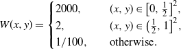 \begin{equation*} W(x,y)= \begin{cases} 2000, & (x,y) \in \big[0,\frac12\big]^2, \\ 2, & (x,y) \in \big(\frac12,1\big]^2, \\ {1}/{100}, \quad & \text{otherwise}. \end{cases} \end{equation*}
It is not difficult to show that the 3-core first appears in the subgraph induced by the vertices that correspond to the bottom-left part, $\big[0,\frac12\big]^2$
, of the graphon, and this emerges near
$\big[0,\frac12\big]^2$
, of the graphon, and this emerges near ${c_3}/{1000}$
, where
${c_3}/{1000}$
, where $c=c_3$
is the threshold of appearance of the 3-core in the binomial random graph on n vertices with edge probability
$c=c_3$
is the threshold of appearance of the 3-core in the binomial random graph on n vertices with edge probability ${c}/{n}$
. It could also be shown that
${c}/{n}$
. It could also be shown that $\mathbb{P}_{X^{\lambda W}}(\mathcal{A})$
has another discontinuity near
$\mathbb{P}_{X^{\lambda W}}(\mathcal{A})$
has another discontinuity near $\lambda=c_3$
, i.e. when the subgraph induced by the vertices that correspond to the top-right part,
$\lambda=c_3$
, i.e. when the subgraph induced by the vertices that correspond to the top-right part, $\big(\frac12,1\big]^2$
, of the graphon will have a 3-core. There is another, more straightforward, way in which a discontinuity could appear in
$\big(\frac12,1\big]^2$
, of the graphon will have a 3-core. There is another, more straightforward, way in which a discontinuity could appear in $\mathbb{P}_{X^{\lambda W}}(\mathcal{A})$
. Consider the graphon
$\mathbb{P}_{X^{\lambda W}}(\mathcal{A})$
. Consider the graphon
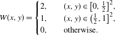 \begin{equation*} W(x,y)= \begin{cases} 2, \quad & (x,y) \in \big[0,\frac12\big]^2, \\ 1, & (x,y) \in \big(\frac12,1\big]^2, \\ 0, & \text{otherwise}. \end{cases} \end{equation*}
It is easy to see that the emergence threshold of the k-core in the subgraph induced by the vertices that correspond to the bottom-left, $\big[0,\frac12\big]^2$
, part of the graphon and the subgraph induced by the vertices that correspond to the top-right part,
$\big[0,\frac12\big]^2$
, part of the graphon and the subgraph induced by the vertices that correspond to the top-right part, $\big(\frac12,1\big]^2$
, of the graphon will be different.
$\big(\frac12,1\big]^2$
, of the graphon will be different.
Remark 2.3. (Paley graphs) Let us give a concrete example where Theorem 2.1 is applicable. Let q be a prime number of the form $4z+1$
with
$4z+1$
with $z\in\mathbb{N}_+$
,
$z\in\mathbb{N}_+$
, $\mathrm{F}_q=\{0,\ldots,q-1\}$
be the finite field, and
$\mathrm{F}_q=\{0,\ldots,q-1\}$
be the finite field, and $\mathrm{F}_q^*=\mathrm{F}_q\setminus\{0\}$
. Consider the sequence of Paley graphs
$\mathrm{F}_q^*=\mathrm{F}_q\setminus\{0\}$
. Consider the sequence of Paley graphs $G_q$
, where the vertex set is
$G_q$
, where the vertex set is $V=\mathrm{F}_q$
and the edge set is given by
$V=\mathrm{F}_q$
and the edge set is given by $E=\{(a,b) \in V \times V\colon a-b \in\mathrm{F}_q^*\times\mathrm{F}_q^*\}$
. Due to [Reference Janson20, Example 10.10],
$E=\{(a,b) \in V \times V\colon a-b \in\mathrm{F}_q^*\times\mathrm{F}_q^*\}$
. Due to [Reference Janson20, Example 10.10], $G_q$
converges to the constant graphon
$G_q$
converges to the constant graphon $\frac12$
in the cut metric as
$\frac12$
in the cut metric as $q \to \infty$
. We can therefore apply Theorem 2.1 and conclude that the size of the k-core in
$q \to \infty$
. We can therefore apply Theorem 2.1 and conclude that the size of the k-core in $G_q(2c/q)$
is asymptotically the same as the size of the k-core in the binomial random graph with q vertices and parameter
$G_q(2c/q)$
is asymptotically the same as the size of the k-core in the binomial random graph with q vertices and parameter $c/q$
(for
$c/q$
(for $c>0$
), except for the threshold of appearance of the k-core. Let us emphasize that the Paley graph is an example of a quasi-random graph, and our result is applicable to any quasi-random graph.
$c>0$
), except for the threshold of appearance of the k-core. Let us emphasize that the Paley graph is an example of a quasi-random graph, and our result is applicable to any quasi-random graph.
As a by-product of the proof of Theorem 2.1, we also obtain a result regarding branching processes that might be of independent interest.
Proposition 2.1. Let $W_n$
be a sequence of graphons such that
$W_n$
be a sequence of graphons such that $d_\square(W_n,W) \rightarrow 0$
. Also, suppose
$d_\square(W_n,W) \rightarrow 0$
. Also, suppose $\lambda \to \mathbb{P}_{X^{\lambda W}}(\mathcal{A})$
is continuous from below at
$\lambda \to \mathbb{P}_{X^{\lambda W}}(\mathcal{A})$
is continuous from below at $\lambda =1$
. Then
$\lambda =1$
. Then $\mathbb{P}_{X^{W_n}}(\mathcal{A}) \rightarrow \mathbb{P}_{X^{W}}(\mathcal{A})$
as
$\mathbb{P}_{X^{W_n}}(\mathcal{A}) \rightarrow \mathbb{P}_{X^{W}}(\mathcal{A})$
as $n\rightarrow\infty$
.
$n\rightarrow\infty$
.
Note that Proposition 2.1 has the following important consequence. The function $\lambda \to \mathbb{P}_{X^{\lambda W}}(\mathcal{A})$
is non-decreasing, and therefore it can have at most countably many discontinuity points. Hence, for almost every positive c, the next corollary provides a way to approximate the order of the k-core using only
$\lambda \to \mathbb{P}_{X^{\lambda W}}(\mathcal{A})$
is non-decreasing, and therefore it can have at most countably many discontinuity points. Hence, for almost every positive c, the next corollary provides a way to approximate the order of the k-core using only $G_n$
.
$G_n$
.
Corollary 2.1. Let $G_n$
be a sequence of graphs with non-negative edge weights which are bounded above by a constant
$G_n$
be a sequence of graphs with non-negative edge weights which are bounded above by a constant $\bar{a}>0$
. Suppose that
$\bar{a}>0$
. Suppose that $G_n$
converges to a graphon W as
$G_n$
converges to a graphon W as $n\rightarrow\infty$
, where
$n\rightarrow\infty$
, where $\lambda\to\mathbb{P}_{X^{\lambda W}}(\mathcal{A})$
is continuous at
$\lambda\to\mathbb{P}_{X^{\lambda W}}(\mathcal{A})$
is continuous at $\lambda =c$
. Then
$\lambda =c$
. Then
 \begin{equation*} C_k(G_n({c}/{n})) = n \mathbb{P}_{X^{cW_{G_n}}}(\mathcal{A}) + o_\mathrm{p}(n). \end{equation*}
Proof of Corollary 2.1. The proof is immediate using Theorem 2.1 and Proposition 2.1.
3. Proof of the upper bound in Theorem 2.1
We will first prove the upper bound, i.e. $C_k(G_n({1}/{n})) \leq n \mathbb{P}_{X^W}(\mathcal{A}) + o_\mathrm{p}(n)$
. The idea is as follows: if a vertex v of a graph is in the k-core, then for any
$C_k(G_n({1}/{n})) \leq n \mathbb{P}_{X^W}(\mathcal{A}) + o_\mathrm{p}(n)$
. The idea is as follows: if a vertex v of a graph is in the k-core, then for any $d>0$
either v has property
$d>0$
either v has property $\mathcal{A}_d$
or v is contained in a cycle of length smaller than 2d. Since the probability of occurrence of short cycles is small for large enough n, the probability that v is in the k-core is bounded above by the probability of having property
$\mathcal{A}_d$
or v is contained in a cycle of length smaller than 2d. Since the probability of occurrence of short cycles is small for large enough n, the probability that v is in the k-core is bounded above by the probability of having property $\mathcal{A}_d$
, ignoring an
$\mathcal{A}_d$
, ignoring an $o_\mathrm{p}(1)$
term. Therefore, to prove the upper bound, we explicitly calculate the probability of event
$o_\mathrm{p}(1)$
term. Therefore, to prove the upper bound, we explicitly calculate the probability of event $\mathcal{A}_d$
using homomorphism density, and a tightness argument. Finally, by letting
$\mathcal{A}_d$
using homomorphism density, and a tightness argument. Finally, by letting $d \to \infty$
, we obtain
$d \to \infty$
, we obtain $C_k(G_n({1}/{n})) \leq n \mathbb{P}_{X^W}(\mathcal{A}) + o_\mathrm{p}(n)$
. Note that we do not need the continuity assumption to show the upper bound.
$C_k(G_n({1}/{n})) \leq n \mathbb{P}_{X^W}(\mathcal{A}) + o_\mathrm{p}(n)$
. Note that we do not need the continuity assumption to show the upper bound.
Let us construct a branching process $^{*}X^{n}$
associated with the random graph
$^{*}X^{n}$
associated with the random graph $G_n({1}/{n})$
.
$G_n({1}/{n})$
. $^*X^n$
has n-types of children,
$^*X^n$
has n-types of children, $1,2,\ldots,n$
. It starts with a single particle whose type is chosen uniformly from
$1,2,\ldots,n$
. It starts with a single particle whose type is chosen uniformly from $1, 2,\ldots, n$
. Conditioning on generation t, each member of generation t has children in the next generation independently of each other, and of everything else. For any particle of type i, its number of children of type j is distributed as Bernoulli
$1, 2,\ldots, n$
. Conditioning on generation t, each member of generation t has children in the next generation independently of each other, and of everything else. For any particle of type i, its number of children of type j is distributed as Bernoulli $(a^n_{i,j}/n)$
.
$(a^n_{i,j}/n)$
.
With some $\rho_n \geq {1}/{n}$
to be determined, we will also use another branching process where, for any particle of type i, its number of children of type j is distributed as Poisson
$\rho_n \geq {1}/{n}$
to be determined, we will also use another branching process where, for any particle of type i, its number of children of type j is distributed as Poisson $(a^n_{i,j}\rho_n)$
. This is actually the branching process associated with the graphon
$(a^n_{i,j}\rho_n)$
. This is actually the branching process associated with the graphon $n\rho_n W_{G_n}$
, and we denote it by
$n\rho_n W_{G_n}$
, and we denote it by $X^{n,\rho_n}$
. By taking
$X^{n,\rho_n}$
. By taking $\rho_n={1}/({n-\bar{a}})$
, the Poisson branching process
$\rho_n={1}/({n-\bar{a}})$
, the Poisson branching process $X^{n, \rho_n}$
stochastically dominates, in the first order,
$X^{n, \rho_n}$
stochastically dominates, in the first order, $^* X^n$
for
$^* X^n$
for $n>3\bar{a}$
. To see this, it is sufficient to show the following inequality for any
$n>3\bar{a}$
. To see this, it is sufficient to show the following inequality for any $i,j \in [n]$
:
$i,j \in [n]$
:
 \begin{align*}\mathbb{P}\big(\text{Poisson}\big(a_{i,j}^n\rho_n\big) > t\big) \geq\mathbb{P}\big(\text{Bernoulli}\big({a_{i,j}^n}/{n}\big) > t\big) \quad \text{for all $t \in \mathbb{Z}$.}\end{align*}
It is trivial for $t\geq 1$
and
$t\geq 1$
and $t<0$
. We need to check only for
$t<0$
. We need to check only for $t=0$
. It can be easily verified that the above inequality is equivalent to
$t=0$
. It can be easily verified that the above inequality is equivalent to
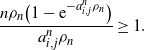 \begin{align*}\frac{n\rho_n\big(1-\mathrm{e}^{-a_{i,j}^n\rho_n}\big)}{a_{i,j}^n\rho_n} \geq 1.\end{align*}
For $n > 3 \bar{a}$
, we have
$n > 3 \bar{a}$
, we have $a_{i,j}^n \rho_n = {a_{i,j}^n}/({n-\bar{a}}) < \frac12$
, and hence, according to the Taylor expansion of
$a_{i,j}^n \rho_n = {a_{i,j}^n}/({n-\bar{a}}) < \frac12$
, and hence, according to the Taylor expansion of $\mathrm{e}^{-a_{i,j}^n \rho_n}$
,
$\mathrm{e}^{-a_{i,j}^n \rho_n}$
,
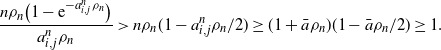 \begin{equation*} \frac{n\rho_n\big(1-\mathrm{e}^{-a_{i,j}^n\rho_n}\big)}{a_{i,j}^n\rho_n} > n\rho_n(1-a_{i,j}^n\rho_n/2) \geq (1+\bar{a}\rho_n)(1-\bar{a}\rho_n/2) \geq 1.\end{equation*}
Note that we can write
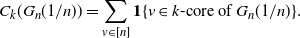 \begin{align*}C_k(G_n({1}/{n})) = \sum_{v\in[n]}{\mathbf{1}}\{v\in\text{\textit{k}-core of }G_n({1}/{n})\}.\end{align*}
If a vertex v is in the k-core, then one of the following two things must be true:
-
(I) v is in a cycle within the d-neighborhood of v (this implies v is in a cycle of length at most 2d);
-
(II) starting from v there is a tree such that v has k neighbors, each of these k neighbors has at least $k-1$
neighbors, and this happens up to generation d. In this case we say vertex v has property
$\mathcal{A}_d$
.
$k-1$
neighbors, and this happens up to generation d. In this case we say vertex v has property
$\mathcal{A}_d$
.


Therefore,
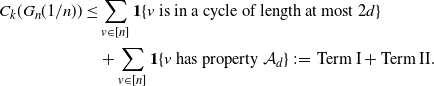 \begin{align} C_k(G_n({1}/{n})) & \leq \sum_{v\in[n]}{\mathbf{1}}\{v\text{ is in a cycle of length at most } 2d\} \notag \\ & \quad + \sum_{v\in[n]}{\mathbf{1}}\{v\text{ has property } \mathcal{A}_d\} \,:\!=\, \text{Term I}+\text{Term II}.\end{align}
Let $V_n$
be a uniformly random variable on
$V_n$
be a uniformly random variable on $\{1,2,\ldots,n\}$
, independent of everything else. Then, according to the construction of
$\{1,2,\ldots,n\}$
, independent of everything else. Then, according to the construction of $G_n({1}/{n})$
and the fact that
$G_n({1}/{n})$
and the fact that $X^{n,\rho_n}$
stochastically dominates
$X^{n,\rho_n}$
stochastically dominates $^{*}X^n$
, we obtain
$^{*}X^n$
, we obtain
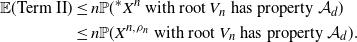 \begin{align} \mathbb{E}(\text{Term II}) & \leq n\mathbb{P}(^{*}X^{n}\text{ with root }V_n\text{ has property }\mathcal{A}_d) \notag \\ & \leq n\mathbb{P}(X^{n,\rho_n}\text{ with root }V_n\text{ has property }\mathcal{A}_d).\end{align}
Before presenting our first proposition, we state an auxiliary result, the van den Berg–Kesten–Reimer (BKR) inequality (see, e.g., [Reference Borgs, Chayes and Randall11]). Consider a product space $\Omega$
of finite sets
$\Omega$
of finite sets $\Omega_1, \dots, \Omega_k$
,
$\Omega_1, \dots, \Omega_k$
, $\Omega = \Omega_1 \times \cdots \times \Omega_k$
. Let
$\Omega = \Omega_1 \times \cdots \times \Omega_k$
. Let $\mathcal{F}= 2^{\Omega}$
, and
$\mathcal{F}= 2^{\Omega}$
, and $\mu$
be a product of k probability measures
$\mu$
be a product of k probability measures $\mu_1, \dots, \mu_k$
. For any configuration
$\mu_1, \dots, \mu_k$
. For any configuration $\omega=(\omega_1, \dots, \omega_k) \in \Omega$
, and any subset S of
$\omega=(\omega_1, \dots, \omega_k) \in \Omega$
, and any subset S of $[k]\,:\!=\,\{1,\dots,k\}$
, we define the cylinder
$[k]\,:\!=\,\{1,\dots,k\}$
, we define the cylinder $[\omega]_S$
by
$[\omega]_S$
by $[\omega]_S \,:\!=\, \{\hat{\omega}\colon\hat{\omega}_i = \omega_i$
for all
$[\omega]_S \,:\!=\, \{\hat{\omega}\colon\hat{\omega}_i = \omega_i$
for all $i \in S\}$
. For any two subsets
$i \in S\}$
. For any two subsets $A, B \subset \Omega$
, define
$A, B \subset \Omega$
, define $A \circ B\,:\!=\, \{\omega\colon\text{there exists some } S=S(\omega) \subset [k]\text{ such that } [\omega]_S \subset A, \, [\omega]_{S^\mathrm{c}} \subset B\}$
.
$A \circ B\,:\!=\, \{\omega\colon\text{there exists some } S=S(\omega) \subset [k]\text{ such that } [\omega]_S \subset A, \, [\omega]_{S^\mathrm{c}} \subset B\}$
.
Lemma 3.1. For any product space $\Omega$
of finite sets, product probability measure
$\Omega$
of finite sets, product probability measure $\mu$
on
$\mu$
on $\Omega$
, and
$\Omega$
, and $A, B \subset \Omega$
, we have the inequality
$A, B \subset \Omega$
, we have the inequality $\mu(A \circ B) \leq \mu(A) \mu(B)$
.
$\mu(A \circ B) \leq \mu(A) \mu(B)$
.
In this paper, to apply the BKR inequality we always take $\Omega^n_{i,j}=\{0,1\}$
,
$\Omega^n_{i,j}=\{0,1\}$
, $i \not= j \in \{1, \dots, n\}$
, and
$i \not= j \in \{1, \dots, n\}$
, and $\Omega = \prod_{i \not= j \in [n]} \Omega^n_{i,j}$
. Then
$\Omega = \prod_{i \not= j \in [n]} \Omega^n_{i,j}$
. Then $\omega^n_{i,j}=1$
means that nodes i and j are linked in the random graph
$\omega^n_{i,j}=1$
means that nodes i and j are linked in the random graph $G_n({1}/{n})$
. According to our construction, we also have
$G_n({1}/{n})$
. According to our construction, we also have $\mu_i(\{1\})= a^n_{i,j}/n$
.
$\mu_i(\{1\})= a^n_{i,j}/n$
.
Proposition 3.1. Let $G_n$
be a sequence of graphs with non-negative edge weights which are bounded above by a constant
$G_n$
be a sequence of graphs with non-negative edge weights which are bounded above by a constant $\bar{a}>0$
. Then, for any fixed d,
$\bar{a}>0$
. Then, for any fixed d,
 \begin{align*}C_k(G_n({1}/{n})) \leq n\mathbb{P}(X^{n,\rho_n}\text{ with root }V_n\text{ has property } \mathcal{A}_d) + o_\mathrm{p}(n).\end{align*}
Proof. According to (3.1) and (3.2), it suffices to show that $\text{Term II} = \mathbb{E}(\text{Term II}) + o_\mathrm{p}(n)$
and
$\text{Term II} = \mathbb{E}(\text{Term II}) + o_\mathrm{p}(n)$
and $\text{Term I}=o_\mathrm{p}(n)$
. In the first two steps, we show the concentration of Term II and its variance, and in the last step we prove that Term I is small.
$\text{Term I}=o_\mathrm{p}(n)$
. In the first two steps, we show the concentration of Term II and its variance, and in the last step we prove that Term I is small.
Step 1. For any two independently and uniformly chosen vertices U and V of $G_n({1}/{n})$
,
$G_n({1}/{n})$
,
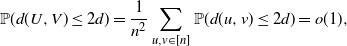 \begin{align*} \mathbb{P}(d(U,V)\leq 2d) = \frac{1}{n^2}\sum_{u,v\in[n]}\mathbb{P}(d(u,v)\leq 2d) = o(1), \end{align*}
where $d(\cdot,\cdot)$
is the graph distance. To see this, note that
$d(\cdot,\cdot)$
is the graph distance. To see this, note that $d(U,V)\leq 2d$
implies there is a path from U to V of length at most 2d. Thus,
$d(U,V)\leq 2d$
implies there is a path from U to V of length at most 2d. Thus,
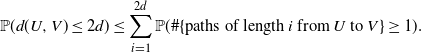 \begin{align*} \mathbb{P}(d(U,V)\leq 2d) \leq \sum_{i=1}^{2d}\mathbb{P}(\#\{\text{paths of length }i\text{ from }U\text{ to } V\} \geq 1). \end{align*}
Using Markov’s inequality we get
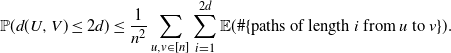 \begin{align*} \mathbb{P}(d(U,V)\leq 2d) \leq \frac{1}{n^2}\sum_{u,v \in [n]}\sum_{i=1}^{2d} \mathbb{E}(\#\{\text{paths of length }i\text{ from }u\text{ to } v\}). \end{align*}
We can get a crude upper bound as
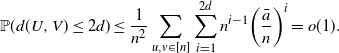 \begin{align*} \mathbb{P}(d(U,V)\leq 2d) \leq \frac{1}{n^2}\sum_{u,v \in [n]}\sum_{i=1}^{2d} n^{i-1}\bigg(\frac{\bar{a}}{n}\bigg)^i = o(1). \end{align*}
Step 2. Let $G^d_n[v]$
be the subgraph of
$G^d_n[v]$
be the subgraph of $G_n({1}/{n})$
induced by the vertices within distance d of
$G_n({1}/{n})$
induced by the vertices within distance d of $v\in[n]$
, and define
$v\in[n]$
, and define $B_{v}=\{\text{root} \, \textit{v} \text{has property }\mathcal{A}_d \text{ in} G^d_n[v]\}$
. It can be easily verified that
$B_{v}=\{\text{root} \, \textit{v} \text{has property }\mathcal{A}_d \text{ in} G^d_n[v]\}$
. It can be easily verified that
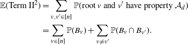 \begin{align} \mathbb{E}({\text{Term II}}^2) & = \sum_{v,v'\in[n]}\mathbb{P}(\text{root }v\text{ and }v'\text{ have property } \mathcal{A}_d) \notag \\ & = \sum_{ v \in [n]} \mathbb{P}(B_v) + \sum_{ v \not = v'} \mathbb{P}(B_v \cap B_{v^{\prime}}). \end{align}
For two different vertices v and v’, we break the probability into two parts:
 \begin{equation*} \mathbb{P}(B_v \cap B_{v^{\prime}}) = \mathbb{P}(B_v \cap B_{v^{\prime}}, d(v,v') \leq 2d) + \mathbb{P}(B_v \cap B_{v^{\prime}}, d(v,v')> 2d ). \end{equation*}
For the second term, it can be easily seen that
 \begin{align*}\{ d(v,v') > 2d\} \cap B_{v} \cap B_{v^{\prime}} \subset \{ d(v,v') > 2d\} \cap B_v \circ B_{v^{\prime}}.\end{align*}
Therefore,
 \begin{align*} \mathbb{P}(B_v \cap B_{v^{\prime}}) & = \mathbb{P}( d(v,v')\leq 2d) + \mathbb{P}(B_{v} \circ B_{v^{\prime}} , d(v,v') > 2d) \\ & \leq \mathbb{P}(d(v,v') \leq 2d) + \mathbb{P}(B_{v} \circ B_{v^{\prime}}). \end{align*}
According to Lemma 3.1, we get $\mathbb{P}(B_{v} \cap B_{v^{\prime}}) \leq \mathbb{P}(d(v,v')\leq2d) + \mathbb{P}(B_{v})\mathbb{P}(B_{v^{\prime}})$
. Combining this with (3.3), we get
$\mathbb{P}(B_{v} \cap B_{v^{\prime}}) \leq \mathbb{P}(d(v,v')\leq2d) + \mathbb{P}(B_{v})\mathbb{P}(B_{v^{\prime}})$
. Combining this with (3.3), we get
 \begin{equation*} \mathbb{E}\big({\text{Term II}}^2\big) \leq n^2\mathbb{P}(d(U,V)\leq2d) + (\mathbb{E}(\text{Term II}))^2 + \sum_{v\in[n]}\big(\mathbb{P}(B_v)-\mathbb{P}(B_v)^2\big). \end{equation*}
Therefore, using Step 1, we get $\mathbb{V}({\text{Term II}}) = o(n^2)$
. Using Chebyshev’s inequality we conclude that
$\mathbb{V}({\text{Term II}}) = o(n^2)$
. Using Chebyshev’s inequality we conclude that $\text{Term II}= \mathbb{E}(\text{Term II})+o_\mathrm{p}(n)$
.
$\text{Term II}= \mathbb{E}(\text{Term II})+o_\mathrm{p}(n)$
.
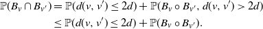
Step 3. We write $C_{v} \,:\!=\, \{v\text{ is in a cycle of length at most }2d\}$
. The first moment of Term I is given by
$C_{v} \,:\!=\, \{v\text{ is in a cycle of length at most }2d\}$
. The first moment of Term I is given by
 \begin{equation} \sum_{v\in[n]}\mathbb{P}(C_v) \leq n\sum_{l=3}^{2d}\frac{(n-1)!}{(n-l)!} \bigg(\frac{\bar{a}}{n}\bigg)^{l} \leq \sum_{l=3}^{2d} \bar{a}^{l} =o(n), \end{equation}
where ${(n-1)!}/{(n-l)!}$
is the number of all possible cycles of length l that contain v, and
${(n-1)!}/{(n-l)!}$
is the number of all possible cycles of length l that contain v, and $({(n-1)!}/{(n-l)!})({\bar{a}}/{n})^{l}$
is an upper bound of the probability that v is in a cycle of length l. Therefore, by Markov’s inequality,
$({(n-1)!}/{(n-l)!})({\bar{a}}/{n})^{l}$
is an upper bound of the probability that v is in a cycle of length l. Therefore, by Markov’s inequality, $\text{Term I}=o_\mathrm{p}(n)$
.
$\text{Term I}=o_\mathrm{p}(n)$
.
3.1. Recursive formula
Let us first fix some notation. For any graphon W, we denote the initial particle of its associated branching process $X^W$
by
$X^W$
by $X^W_0$
, the type of
$X^W_0$
, the type of $X^W_0$
by
$X^W_0$
by $T(W)_0$
, and the first generation by
$T(W)_0$
, and the first generation by $X^W_{\{1\}},\dots,X^W_{\{N(W)_0\}}$
, where
$X^W_{\{1\}},\dots,X^W_{\{N(W)_0\}}$
, where $N(W)_0$
is the number of children of
$N(W)_0$
is the number of children of $X^W_0$
. For
$X^W_0$
. For $d\geq 2$
, we denote each element in the dth generation by
$d\geq 2$
, we denote each element in the dth generation by $X^W_{\{i_1|i_2|\cdots|i_d\}}$
if it is the
$X^W_{\{i_1|i_2|\cdots|i_d\}}$
if it is the $i_d$
th child of
$i_d$
th child of $X^W_{\{i_1|i_2|\cdots|i_{d-1}\}}$
. Denote the number of children of
$X^W_{\{i_1|i_2|\cdots|i_{d-1}\}}$
. Denote the number of children of $X^W_{\{i_1|i_2|\cdots|i_d\}}$
by
$X^W_{\{i_1|i_2|\cdots|i_d\}}$
by $N(W)_{\{i_1|i_2|\cdots|i_d\}}$
, and the type of
$N(W)_{\{i_1|i_2|\cdots|i_d\}}$
, and the type of $X^W_{\{i_1|i_2|\cdots|i_d\}}$
by
$X^W_{\{i_1|i_2|\cdots|i_d\}}$
by $T(W)_{\{i_1|i_2|\cdots|i_d\}}$
. Let
$T(W)_{\{i_1|i_2|\cdots|i_d\}}$
. Let ${\mathbf{N}}(W)^d$
denote the tree formed by the first d generations of
${\mathbf{N}}(W)^d$
denote the tree formed by the first d generations of $X^W$
.
$X^W$
.
Let ${\mathbf{K}}$
be a tree and
${\mathbf{K}}$
be a tree and $\mathrm{h}({\mathbf{K}})$
the height of the tree
$\mathrm{h}({\mathbf{K}})$
the height of the tree ${\mathbf{K}}$
. We define
${\mathbf{K}}$
. We define $g(x,{\mathbf{K}})\,:\!=\,\mathbb{P}({\mathbf{N}}(W)^{\mathrm{h}({\mathbf{K}})}={\mathbf{K}}\mid T(W)_0=x)$
. It is clear that
$g(x,{\mathbf{K}})\,:\!=\,\mathbb{P}({\mathbf{N}}(W)^{\mathrm{h}({\mathbf{K}})}={\mathbf{K}}\mid T(W)_0=x)$
. It is clear that $\mathbb{P}({\mathbf{N}}(W)^{\mathrm{h}({\mathbf{K}})}={\mathbf{K}})=\int g(x,{\mathbf{K}})\,\mathrm{d} x$
.
$\mathbb{P}({\mathbf{N}}(W)^{\mathrm{h}({\mathbf{K}})}={\mathbf{K}})=\int g(x,{\mathbf{K}})\,\mathrm{d} x$
.
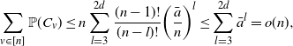
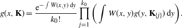
Proposition 3.2.
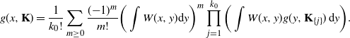
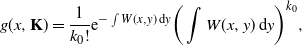
 \begin{equation} g(x,{\mathbf{K}}) = \frac{\mathrm{e}^{-\int W(x,y)\,\mathrm{d} y}}{k_0!} \prod_{j=1}^{k_0}\bigg(\int W(x,y)g(y,{\mathbf{K}}_{\{j\}})\,\mathrm{d} y\bigg), \end{equation}
where $k_0$
is the number of the first generation in
$k_0$
is the number of the first generation in ${\mathbf{K}}$
, and
${\mathbf{K}}$
, and ${\mathbf{K}}_{\{j\}}$
is the subtree of
${\mathbf{K}}_{\{j\}}$
is the subtree of ${\mathbf{K}}$
whose root is the jth member of the elements of the first generation of
${\mathbf{K}}$
whose root is the jth member of the elements of the first generation of ${\mathbf{K}}$
.
${\mathbf{K}}$
.
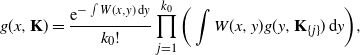
Proof. When $\mathrm{h}({\mathbf{K}})=1$
, it can be easily seen that
$\mathrm{h}({\mathbf{K}})=1$
, it can be easily seen that
 \begin{align*}g(x,{\mathbf{K}}) = \frac{1}{k_0!}\mathrm{e}^{-\int W(x,y)\,\mathrm{d} y}\bigg(\int W(x,y)\,\mathrm{d} y\bigg)^{k_0}.\end{align*}
For $\mathrm{h}({\mathbf{K}}) \geq 2$
, we get
$\mathrm{h}({\mathbf{K}}) \geq 2$
, we get
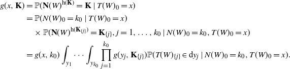 \begin{align*} g(x,{\mathbf{K}}) & = \mathbb{P}({\mathbf{N}}(W)^{\mathrm{h}({\mathbf{K}})} = {\mathbf{K}} \mid T(W)_0=x) \\ & = \mathbb{P}(N(W)_0=k_0\mid T(W)_0=x) \\ & \quad \times \mathbb{P}({\mathbf{N}}(W)^{\mathrm{h}({\mathbf{K}}_{\{j\}})} = {\mathbf{K}}_{\{j\}}, j=1,\dots,k_0 \mid N(W)_0=k_0,T(W)_0=x) \\ & = g(x,k_0) \int_{y_1} \cdots \int_{y_{k_0}} \prod_{j=1}^{k_0} g(y_j,{\mathbf{K}}_{\{j\}})\mathbb{P}(T(W)_{\{j\}} \in \mathrm{d} y_j\mid N(W)_0=k_0, T(W)_0=x) . \end{align*}
Here we have used $\prod_{j=1}^{k_0} g(y_j, {\mathbf{K}}_{\{j\}}) \mathbb{P}(T(W)_{\{j\}} \in \mathrm{d} y_j\mid N(W)_0=k_0, T(W)_0=x)$
to denote the following density:
$\prod_{j=1}^{k_0} g(y_j, {\mathbf{K}}_{\{j\}}) \mathbb{P}(T(W)_{\{j\}} \in \mathrm{d} y_j\mid N(W)_0=k_0, T(W)_0=x)$
to denote the following density:
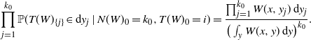 \begin{equation*} \prod_{j=1}^{k_0} \mathbb{P}(T(W)_{\{j\}} \in \mathrm{d} y_j\mid N(W)_0 =k_0, T(W)_0=i) = \frac{\prod_{j=1}^{k_0} W(x, y_j) \, \mathrm{d} y_j }{ \big(\int_y W(x,y) \, \mathrm{d} y\big)^{k_0} }. \end{equation*}
Therefore, we obtain the recursive formula
 \begin{equation*} g(x,{\mathbf{K}}) = \frac{\mathrm{e}^{-\int W(x,y)\,\mathrm{d} y}}{k_0!} \prod_{j=1}^{k_0}\bigg(\int W(x,y)g(y,{\mathbf{K}}_{\{j\}})\,\mathrm{d} y\bigg). \end{equation*}
3.2. Convergence
Let $W_n$
be a sequence of graphons such that
$W_n$
be a sequence of graphons such that $d_\square(W_n,W) \to 0$
and
$d_\square(W_n,W) \to 0$
and $\sup_{n,x,y} W_n(x,y) \leq \bar{a}$
for some positive constant
$\sup_{n,x,y} W_n(x,y) \leq \bar{a}$
for some positive constant $\bar{a}$
. Let
$\bar{a}$
. Let $X^{W_n}$
be the associated branching process of
$X^{W_n}$
be the associated branching process of $W_n$
, and
$W_n$
, and $g_n(x,{\mathbf{K}})=\mathbb{P}( {\mathbf{N}}(W_n)^{\mathrm{h}({\mathbf{K}})}= {\mathbf{K}}\mid T(W_n)_0 =x)$
.
$g_n(x,{\mathbf{K}})=\mathbb{P}( {\mathbf{N}}(W_n)^{\mathrm{h}({\mathbf{K}})}= {\mathbf{K}}\mid T(W_n)_0 =x)$
.
We want to show that, as $n \to \infty$
,
$n \to \infty$
, $\int g_n(x,{\mathbf{K}}) \, \mathrm{d} x \to \int g(x,{\mathbf{K}}) \, \mathrm{d} x$
. To see this, for any graphon W, any finite tree T with root 0, and any
$\int g_n(x,{\mathbf{K}}) \, \mathrm{d} x \to \int g(x,{\mathbf{K}}) \, \mathrm{d} x$
. To see this, for any graphon W, any finite tree T with root 0, and any $x \in [0,1]$
, we define the vertex-prescribed homomorphism density
$x \in [0,1]$
, we define the vertex-prescribed homomorphism density
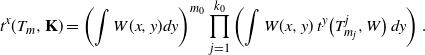
 \begin{equation*} t^x(T,W) = \int_{[0,1]^{|V(T)|-1}}\prod_{i\in E(T)}W(x,x_i) \prod_{ij\in E(T),i,j\geq1}W(x_i,x_j)\,\mathrm{d} x_1 \cdots \mathrm{d} x_{|V(T)|-1}\end{equation*}
and the homomorphism density $t(T,W)=\int_{[0,1]} t^x(T,W) \, \mathrm{d} x$
. It is well known that, for finite T,
$t(T,W)=\int_{[0,1]} t^x(T,W) \, \mathrm{d} x$
. It is well known that, for finite T, $t(T,W_n) \to t(T,W)$
as long as
$t(T,W_n) \to t(T,W)$
as long as $d_\square(W_n,W) \to 0$
; see, e.g., [Reference Borgs, Chayes, Lovász, Sós and Vesztergombi9, Reference Borgs, Chayes, Lovász, Sós and Vesztergombi10, Reference Lovász and Szegedy27]. We will rewrite
$d_\square(W_n,W) \to 0$
; see, e.g., [Reference Borgs, Chayes, Lovász, Sós and Vesztergombi9, Reference Borgs, Chayes, Lovász, Sós and Vesztergombi10, Reference Lovász and Szegedy27]. We will rewrite $\int g_n(x,{\mathbf{K}}) \, \mathrm{d} x $
and
$\int g_n(x,{\mathbf{K}}) \, \mathrm{d} x $
and $\int g(x, {\mathbf{K}}) \,\mathrm{d} x$
as
$\int g(x, {\mathbf{K}}) \,\mathrm{d} x$
as $\sum_{m \geq 0} \lambda_m t(T_m,W_n)$
and
$\sum_{m \geq 0} \lambda_m t(T_m,W_n)$
and $\sum_{m \geq 0} \lambda_m t(T_m,W)$
respectively for a sequence of trees
$\sum_{m \geq 0} \lambda_m t(T_m,W)$
respectively for a sequence of trees $T_m$
.
$T_m$
.
Proposition 3.3. For any $\bar{a} >0$
and any
$\bar{a} >0$
and any ${\mathbf{K}}$
with
${\mathbf{K}}$
with $\mathrm{h}({\mathbf{K}})=d<\infty$
, there exists a sequence of finite trees
$\mathrm{h}({\mathbf{K}})=d<\infty$
, there exists a sequence of finite trees $(T_m)_{m \geq 0}$
and a sequence of real numbers
$(T_m)_{m \geq 0}$
and a sequence of real numbers $(\lambda_m)_{m \geq 0}$
such that, for any graphon W with
$(\lambda_m)_{m \geq 0}$
such that, for any graphon W with $\sup_{x,y} W(x,y) \leq \bar{a}$
,
$\sup_{x,y} W(x,y) \leq \bar{a}$
,
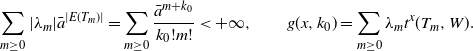
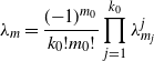
-
(i)
$\sum_{m \geq 0} |\lambda_m| \bar{a}^{|E(T_m)|}<+\infty$
; -
(ii)
$g(x,{\mathbf{K}})=\sum_{m \geq 0} \lambda_m t^x(T_m,W)$
.


Proof. We proceed by induction. For $d=1$
,
$d=1$
,
 \begin{equation*} g(x,{\mathbf{K}}) = \frac{1}{k_0!}\mathrm{e}^{-\int W(x,y)\,\mathrm{d} y}\bigg(\int W(x,y)\,\mathrm{d} y\bigg)^{k_0} = \frac{1}{k_0!}\sum_{m=0}\frac{({-}1)^m}{m!}\bigg(\int W(x,y)\,\mathrm{d} y\bigg)^{m+k_0}, \end{equation*}
where $k_0$
is the number of the first generation in
$k_0$
is the number of the first generation in ${\mathbf{K}}$
. For any
${\mathbf{K}}$
. For any $m\in\mathbb{N}$
, take
$m\in\mathbb{N}$
, take $T_m$
to be an
$T_m$
to be an $(m+k_0)$
-star, i.e. a tree of height 1 with
$(m+k_0)$
-star, i.e. a tree of height 1 with $(m+k_0)$
leaves. Define
$(m+k_0)$
leaves. Define $\lambda_m\,:\!=\, {({-}1)^m}/({k_0!m!})$
. Then it can be easily seen that
$\lambda_m\,:\!=\, {({-}1)^m}/({k_0!m!})$
. Then it can be easily seen that
 \begin{align*} \sum_{m \geq 0}|\lambda_m|\bar{a}^{|E(T_m)|} = \sum_{m \geq 0}\frac{\bar{a}^{m+k_0}}{k_0!m!} < +\infty, \qquad g(x,k_0)=\sum_{ m \geq 0} \lambda_m t^x(T_m,W). \end{align*}
Now suppose that our claim is true for any configuration ${\mathbf{K}}^{d-1}$
. Using our recursive formula in (3.5), we expand the exponential term and obtain
${\mathbf{K}}^{d-1}$
. Using our recursive formula in (3.5), we expand the exponential term and obtain
 \begin{equation*} g(x,{\mathbf{K}}) = \frac{1}{k_0!}\sum_{m\geq0}\frac{({-}1)^m}{m!}\bigg(\int W(x,y)\mathrm{d} y\bigg)^m \prod_{j=1}^{k_0}\bigg(\int W(x,y)g(y,{\mathbf{K}}_{\{j\}})\,\mathrm{d} y\bigg). \end{equation*}
For each ${\mathbf{K}}_{\{j\}}, j=1,\dots,k_0$
, we have sequences
${\mathbf{K}}_{\{j\}}, j=1,\dots,k_0$
, we have sequences $\big(\lambda_m^j\big)_{m \geq 0}, \big(T^j_m\big)_{m \geq 0}$
such that our claim is satisfied. For each
$\big(\lambda_m^j\big)_{m \geq 0}, \big(T^j_m\big)_{m \geq 0}$
such that our claim is satisfied. For each $m=(m_0, m_1, \dots, m_{k_0}) \in \mathbb{N}^{k_0+1}$
, we define
$m=(m_0, m_1, \dots, m_{k_0}) \in \mathbb{N}^{k_0+1}$
, we define
 \begin{align*}\lambda_m=\frac{({-}1)^{m_0}}{k_0!m_0!}\prod_{j=1}^{k_0}\lambda_{m_j}^{j}\end{align*}
and tree $T_m$
as in Figure 1. In
$T_m$
as in Figure 1. In $T_m$
,
$T_m$
, $m_0$
stands for the number of leaves attached to the root, and the additional trees
$m_0$
stands for the number of leaves attached to the root, and the additional trees $T^i_{m_i}$
,
$T^i_{m_i}$
, $i=1,\dots,k_0$
, are linked to the root. It is then clear that
$i=1,\dots,k_0$
, are linked to the root. It is then clear that
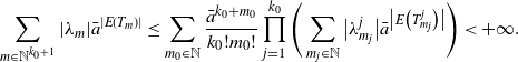 \begin{equation*} \sum_{m\in\mathbb{N}^{k_0+1}}|\lambda_m|\bar{a}^{|E(T_m)|} \leq \sum_{m_0\in\mathbb{N}}\frac{\bar{a}^{k_0+m_0}}{k_0!m_0!} \prod_{j=1}^{k_0}\Bigg(\sum_{m_j\in\mathbb{N}}\big|\lambda_{m_j}^{j}\big|\bar{a}^{\big|E\big(T_{m_j}^j\big)\big|}\Bigg) < +\infty. \end{equation*}
According to our induction, we have $g(y,{\mathbf{K}}_{\{j\}}) = \sum_{m_j \geq 0} \lambda_{m_j}^{j}t^y\big(T^j_{m_j},W\big)$
. Therefore, we obtain
$g(y,{\mathbf{K}}_{\{j\}}) = \sum_{m_j \geq 0} \lambda_{m_j}^{j}t^y\big(T^j_{m_j},W\big)$
. Therefore, we obtain
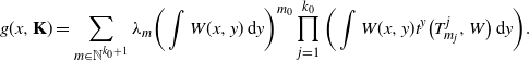 \begin{equation*} g(x,{\mathbf{K}}) = \sum_{m\in\mathbb{N}^{k_0+1}}\lambda_m\bigg(\int W(x,y)\,\mathrm{d} y\bigg)^{m_0} \prod_{j=1}^{k_0}\bigg(\int W(x,y)t^y\big(T_{m_j}^j,W\big)\,\mathrm{d} y\bigg). \end{equation*}
It can be easily verified that, for each $m \in \mathbb{N}^{k_0+1}$
,
$m \in \mathbb{N}^{k_0+1}$
,
 \begin{equation*} t^x(T_m, {\mathbf{K}}) =\left(\int W(x,y) dy\right)^{m_0} \prod_{j=1}^{k_0} \left(\int W(x,y)\, t^y\big(T_{m_j}^j, W\big) \,dy \right). \end{equation*}
Thus, we conclude that $g(x,{\mathbf{K}}) = \sum_{m\in\mathbb{N}^{k_0+1}}\lambda_m t^x(T_m,W)$
.
$g(x,{\mathbf{K}}) = \sum_{m\in\mathbb{N}^{k_0+1}}\lambda_m t^x(T_m,W)$
.
Figure 1. Tree $T_m$
.
$T_m$
.
Proposition 3.4. Suppose $W_n$
is a sequence of graphons such that
$W_n$
is a sequence of graphons such that $d_\square(W_n,W) \to 0$
satisfying
$d_\square(W_n,W) \to 0$
satisfying $\sup_{n,x,y}W_n(x,y) \leq \bar{a}$
for some positive constant
$\sup_{n,x,y}W_n(x,y) \leq \bar{a}$
for some positive constant $\bar{a}$
. Let
$\bar{a}$
. Let ${\mathbf{K}}^d$
be a tree of height d. Then
${\mathbf{K}}^d$
be a tree of height d. Then $\lim_{n\to\infty}\mathbb{P}\big({\mathbf{N}}(W_n)^d = {\mathbf{K}}^d\big) = \mathbb{P}({\mathbf{N}}(W)^d = {\mathbf{K}}^d)$
.
$\lim_{n\to\infty}\mathbb{P}\big({\mathbf{N}}(W_n)^d = {\mathbf{K}}^d\big) = \mathbb{P}({\mathbf{N}}(W)^d = {\mathbf{K}}^d)$
.
Proof. According to Proposition 3.3, we get
 \begin{align*} \mathbb{P}\big({\mathbf{N}}(W_n)^d = {\mathbf{K}}^d\big) & = \int g_n\big(x,{\mathbf{K}}^d\big)\,\mathrm{d} x = \sum_{m\geq1}\lambda_mt(T_m,W_n), \\ \mathbb{P}\big({\mathbf{N}}(W)^d = {\mathbf{K}}^d\big) & = \int g\big(x,{\mathbf{K}}^d\big)\,\mathrm{d} x = \sum_{m\geq1}\lambda_mt(T_m,W). \end{align*}
Since $W_n$
converges to W in that cut norm,
$W_n$
converges to W in that cut norm, $t(T_m,W_n) \to t(T_m, W)$
as
$t(T_m,W_n) \to t(T_m, W)$
as $n \to \infty$
. Due to the uniform bound
$n \to \infty$
. Due to the uniform bound
 \begin{align*}\sum_{m\geq1}\lambda_mt(T_m,W_n)\leq\sum_{m\geq1}\lambda_m\bar{a}^{|E(T_m)|} < +\infty,\end{align*}
we apply the dominated convergence theorem and conclude that $\mathbb{P}\big({\mathbf{N}}(W_n)^d={\mathbf{K}}^d\big)$
converges to
$\mathbb{P}\big({\mathbf{N}}(W_n)^d={\mathbf{K}}^d\big)$
converges to $\mathbb{P}\big({\mathbf{N}}(W)^d={\mathbf{K}}^d\big) $
as
$\mathbb{P}\big({\mathbf{N}}(W)^d={\mathbf{K}}^d\big) $
as $n \to \infty$
.
$n \to \infty$
.
3.3. Tightness
Notice that $X^W \in \mathcal{A}_d$
is equivalent to
$X^W \in \mathcal{A}_d$
is equivalent to ${\mathbf{N}}(W)^d \in \mathcal{A}_d$
. To make our computation clear, we will sometimes adopt the latter notation. Recall that we want to show that
${\mathbf{N}}(W)^d \in \mathcal{A}_d$
. To make our computation clear, we will sometimes adopt the latter notation. Recall that we want to show that
 \begin{equation*} \mathbb{P}\big({\mathbf{N}}(W)^d \in \mathcal{A}_d\big) = \lim\limits_{n \to \infty} \mathbb{P}\big({\mathbf{N}}(W_n)^d \in \mathcal{A}_d\big).\end{equation*}
To apply Proposition 3.4, we need a tightness result. For $K \in \mathbb{N}$
, we define
$K \in \mathbb{N}$
, we define ${\mathbf{N}}(W)^d \leq K$
if
${\mathbf{N}}(W)^d \leq K$
if $N(W)_{\{i_1|i_2|\cdots|i_j\}} \leq K$
for any
$N(W)_{\{i_1|i_2|\cdots|i_j\}} \leq K$
for any $X^W_{\{i_1|i_2|\cdots|i_j\}}$
in the first d generations.
$X^W_{\{i_1|i_2|\cdots|i_j\}}$
in the first d generations.
Lemma 3.2. Suppose $\sup_{x,y}W(x,y) \leq \bar{a}$
for some positive constant
$\sup_{x,y}W(x,y) \leq \bar{a}$
for some positive constant $\bar{a}$
. Then, for any
$\bar{a}$
. Then, for any $\alpha>0$
,
$\alpha>0$
, $d \in \mathbb{N}$
, there exists a large enough
$d \in \mathbb{N}$
, there exists a large enough $K_0 \in \mathbb{N}$
uniformly for
$K_0 \in \mathbb{N}$
uniformly for $x \in [0,1]$
such that
$x \in [0,1]$
such that $K \geq K_0$
implies
$K \geq K_0$
implies $\mathbb{P}({\mathbf{N}}(W)^d \leq K \mid T(W)_0 = x) > 1 - (1/K)^{\alpha}$
. Here, the choice of
$\mathbb{P}({\mathbf{N}}(W)^d \leq K \mid T(W)_0 = x) > 1 - (1/K)^{\alpha}$
. Here, the choice of $K_0$
only depends on
$K_0$
only depends on $\alpha$
, d, and
$\alpha$
, d, and $\bar{a}$
.
$\bar{a}$
.
Proof. We prove the result by induction. Recall that when $\mathrm{h}({\mathbf{K}})=1$
, we have
$\mathrm{h}({\mathbf{K}})=1$
, we have
 \begin{align*}g(x,{\mathbf{K}})=\frac{1}{k_0!}\mathrm{e}^{-\int W(x,y)\,\mathrm{d} y}\bigg(\int W(x,y)\,\mathrm{d} y\bigg)^{k_0},\end{align*}
where $k_0$
is the number of the first generation in
$k_0$
is the number of the first generation in ${\mathbf{K}}$
. For any
${\mathbf{K}}$
. For any $k\in\mathbb{N}$
, we define, for
$k\in\mathbb{N}$
, we define, for $c \in \mathbb{R}_+$
,
$c \in \mathbb{R}_+$
, $\psi_{k}(c) \,:\!=\, \sum_{l=k+1}^{\infty} ({1}/{l!}) \mathrm{e}^{-c} c^l$
. Thus we have
$\psi_{k}(c) \,:\!=\, \sum_{l=k+1}^{\infty} ({1}/{l!}) \mathrm{e}^{-c} c^l$
. Thus we have
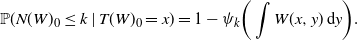 \begin{equation*} \mathbb{P}(N(W)_0 \leq k \mid T(W)_0=x) = 1 - \psi_k \bigg(\int W(x,y)\,\mathrm{d} y\bigg). \end{equation*}
It can be easily verified that $\psi^{\prime}_k(c)={\mathrm{e}^{-c}c^{k}}/{k!} \geq 0$
, and hence
$\psi^{\prime}_k(c)={\mathrm{e}^{-c}c^{k}}/{k!} \geq 0$
, and hence $\psi_k\big(\int W(x,y)\,\mathrm{d} y\big) \leq \psi_k(\bar{a})$
. Choosing K large enough that
$\psi_k\big(\int W(x,y)\,\mathrm{d} y\big) \leq \psi_k(\bar{a})$
. Choosing K large enough that $\psi_K(\bar{a}) <K^{-\alpha}$
is indeed possible, it is clear that
$\psi_K(\bar{a}) <K^{-\alpha}$
is indeed possible, it is clear that
 \begin{equation*} \mathbb{P}(N(W)_0 \leq K \mid T(X^n)_0=x) = 1 - \psi_K\bigg(\int W(x,y)\,\mathrm{d} y\bigg) > 1 - (1/K)^{\alpha}. \end{equation*}
Assume our claim is true for $d-1$
. Then, for any
$d-1$
. Then, for any $\beta >0$
, there exists a K such that
$\beta >0$
, there exists a K such that
 \begin{align*}\mathbb{P}({\mathbf{N}}(W)^d_{\{j\}} \leq K \mid T(W)^d_{\{j\}}=y) \geq 1 - (1/K)^{\beta}.\end{align*}
Note that
 \begin{align*} \mathbb{P}\big({\mathbf{N}}(W)^d \leq K \mid T(W)_0=x\big) & = \sum_{k=0}^{K}\mathbb{P}\big({\mathbf{N}}(W)^d_{\{j\}}\leq K,j=1,\dots,k\mid N(W)_0=k,T(W)_0=x\big) \\ & \quad \times \mathbb{P}(N(W)_0=k \mid T(W)_0=x). \end{align*}
As in the proof of Proposition 3.2, we have
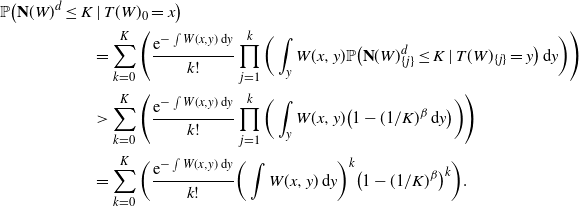 \begin{align*} \mathbb{P}\big({\mathbf{N}}(W)^d \leq K & \mid T(W)_0=x\big) \\ & = \sum_{k=0}^{K}\Bigg(\frac{\mathrm{e}^{-\int W(x,y)\,\mathrm{d} y}}{k!}\prod_{j=1}^{k} \bigg(\int_y W(x,y)\mathbb{P}\big({\mathbf{N}}(W)^d_{\{j\}} \leq K \mid T(W)_{\{j\}}=y\big)\,\mathrm{d} y\bigg) \Bigg) \\ & > \sum_{k=0}^{K}\Bigg(\frac{\mathrm{e}^{-\int W(x,y)\,\mathrm{d} y}}{k!}\prod_{j=1}^{k} \bigg(\int_y W(x,y) \big(1-(1/K)^{\beta}\,\mathrm{d} y\big)\bigg)\Bigg) \\ & = \sum_{k=0}^{K}\bigg(\frac{\mathrm{e}^{-\int W(x,y)\,\mathrm{d} y}}{k!}\bigg(\int W(x,y)\,\mathrm{d} y\bigg)^k \big(1-(1/K)^{\beta}\big)^k\bigg). \end{align*}
Since $(1-(1/K)^{\beta})^K > 1- (1/K)^{\beta-2}$
for large K, we have
$(1-(1/K)^{\beta})^K > 1- (1/K)^{\beta-2}$
for large K, we have
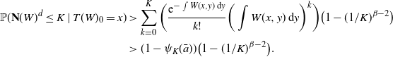 \begin{align*} \mathbb{P}({\mathbf{N}}(W)^d \leq K \mid T(W)_0=x) & > \sum_{k=0}^{K}\bigg(\frac{\mathrm{e}^{-\int W(x,y)\,\mathrm{d} y}}{k!}\bigg(\int W(x,y)\,\mathrm{d} y\bigg)^k\bigg) \big(1- (1/K)^{\beta -2}\big) \\ & > (1-\psi_K(\bar{a}))\big(1- (1/K)^{\beta -2}\big). \end{align*}
Therefore, by taking $\beta =\alpha+3$
, and large K such that
$\beta =\alpha+3$
, and large K such that $\psi_K(\bar{a}) < (1/K)^{\alpha+1}$
, we conclude that
$\psi_K(\bar{a}) < (1/K)^{\alpha+1}$
, we conclude that $\mathbb{P} ({\mathbf{N}}(W)^d \leq K \mid T(W)_0 =x) > 1- (1/K)^{\alpha}$
.
$\mathbb{P} ({\mathbf{N}}(W)^d \leq K \mid T(W)_0 =x) > 1- (1/K)^{\alpha}$
.
Proposition 3.5. Suppose $W_n$
is a sequence of graphons such that
$W_n$
is a sequence of graphons such that $d_\square(W_n,W) \to 0$
and satisfying
$d_\square(W_n,W) \to 0$
and satisfying $\sup_{n,x,y} W_n(x,y) \leq \bar{a}$
for some positive constant
$\sup_{n,x,y} W_n(x,y) \leq \bar{a}$
for some positive constant $\bar{a}$
. Then, for any fixed d, we have
$\bar{a}$
. Then, for any fixed d, we have $\lim_{n\to\infty}\mathbb{P}({\mathbf{N}}(W_n)^d\in\mathcal{A}_d) = \mathbb{P}({\mathbf{N}}(W)^d\in\mathcal{A}_d)$
, from which we conclude that
$\lim_{n\to\infty}\mathbb{P}({\mathbf{N}}(W_n)^d\in\mathcal{A}_d) = \mathbb{P}({\mathbf{N}}(W)^d\in\mathcal{A}_d)$
, from which we conclude that $\limsup_{n\to\infty}\mathbb{P}_{X^{W_n}}(\mathcal{A})\leq\mathbb{P}_{X^W}(\mathcal{A})$
.
$\limsup_{n\to\infty}\mathbb{P}_{X^{W_n}}(\mathcal{A})\leq\mathbb{P}_{X^W}(\mathcal{A})$
.
Proof. Due to Proposition 3.4, it can be seen that, for fixed d, K,
 \begin{equation*} \lim_{n\to\infty}\mathbb{P}\big({\mathbf{N}}(W_n)^d\in\mathcal{A}_d,{\mathbf{N}}(W_n)^d \leq K\big) = \mathbb{P}\big({\mathbf{N}}(W)^d \in \mathcal{A}_d, {\mathbf{N}}(W)^d \leq K\big). \end{equation*}
Applying Lemma 3.2, we let $K \to \infty$
and obtain
$K \to \infty$
and obtain $\lim_{n\to\infty}\mathbb{P}\big({\mathbf{N}}(W_n)^d\in\mathcal{A}_d\big) = \mathbb{P}\big({\mathbf{N}}(W)^d \in \mathcal{A}_d\big)$
.
$\lim_{n\to\infty}\mathbb{P}\big({\mathbf{N}}(W_n)^d\in\mathcal{A}_d\big) = \mathbb{P}\big({\mathbf{N}}(W)^d \in \mathcal{A}_d\big)$
.
For any $\epsilon >0$
, there exists a d such that
$\epsilon >0$
, there exists a d such that $\mathbb{P}\big({\mathbf{N}}(W)^d \in \mathcal{A}_d\big)=\mathbb{P}\big(X^W \in \mathcal{A}_d\big) \leq \mathbb{P}_{X^W}(\mathcal{A})+\epsilon$
. It can then be easily verified that
$\mathbb{P}\big({\mathbf{N}}(W)^d \in \mathcal{A}_d\big)=\mathbb{P}\big(X^W \in \mathcal{A}_d\big) \leq \mathbb{P}_{X^W}(\mathcal{A})+\epsilon$
. It can then be easily verified that
 \begin{equation*} \limsup_{n\to\infty}\mathbb{P}_{X^{W_n}}(\mathcal{A}) \leq \limsup_{n\to\infty}\mathbb{P}\big({\mathbf{N}}({W_n})^d \in \mathcal{A}_d\big) = \mathbb{P}\big({\mathbf{N}}(W)^d \in \mathcal{A}_d\big) \leq \mathbb{P}_{X^W}(\mathcal{A})+\epsilon. \end{equation*}
Therefore, we obtain $\limsup_{n\to\infty}\mathbb{P}_{X^{W_n}}(\mathcal{A}) \leq \mathbb{P}_{X^W}(\mathcal{A})$
.
$\limsup_{n\to\infty}\mathbb{P}_{X^{W_n}}(\mathcal{A}) \leq \mathbb{P}_{X^W}(\mathcal{A})$
.
3.4. Completing the proof of the upper bound
Recalling Proposition 3.1, we have $C_k(G_n({1}/{n})\leq n\mathbb{P}(X^{n,\rho_n} \in \mathcal{A}_d) + o_\mathrm{p}(n)$
. Note that
$C_k(G_n({1}/{n})\leq n\mathbb{P}(X^{n,\rho_n} \in \mathcal{A}_d) + o_\mathrm{p}(n)$
. Note that $X^{n,\rho_n}$
is the branching process associated with the graphon
$X^{n,\rho_n}$
is the branching process associated with the graphon $n\rho_n W_{G_n}$
,
$n\rho_n W_{G_n}$
, $d_\square ( W_{G_n}, W) \to 0$
, and
$d_\square ( W_{G_n}, W) \to 0$
, and $n\rho_n \to 1$
. Applying Proposition 3.5 with
$n\rho_n \to 1$
. Applying Proposition 3.5 with $W_n = n\rho_n W_{G_n}$
, we obtain that
$W_n = n\rho_n W_{G_n}$
, we obtain that $C_k(G_n({1}/{n})) \leq n \mathbb{P}_{X^W}(\mathcal{A}_d) + o_\mathrm{p}(n)$
. Letting
$C_k(G_n({1}/{n})) \leq n \mathbb{P}_{X^W}(\mathcal{A}_d) + o_\mathrm{p}(n)$
. Letting $d \to \infty$
in the above inequality, we have our result.
$d \to \infty$
in the above inequality, we have our result.
4. The proof of the lower bound in Theorem 2.1
Before proceeding to our proof of the lower bound, we argue that it suffices to prove it for irreducible W. A graphon W is said to be irreducible if there is no measurable $A \subset [0,1]$
such that
$A \subset [0,1]$
such that $\text{Leb}(A) \in (0,1)$
and
$\text{Leb}(A) \in (0,1)$
and $W=0$
almost everywhere on
$W=0$
almost everywhere on $A\times A^\mathrm{c}$
, where
$A\times A^\mathrm{c}$
, where $\text{Leb}(A)$
stands for the Lebesgue measure of A.
$\text{Leb}(A)$
stands for the Lebesgue measure of A.
According to [Reference Bollobás, Janson and Riordan7, Lemma 5.17], for any graphon W, there exists a partition $[0,1]=\cup_{i=1}^N I_i$
with
$[0,1]=\cup_{i=1}^N I_i$
with $0 \leq N \leq \infty$
such that
$0 \leq N \leq \infty$
such that $\text{Leb}(I_i) >0$
for each
$\text{Leb}(I_i) >0$
for each $i \geq 1$
, the restriction of W on
$i \geq 1$
, the restriction of W on $I_i \times I_i$
is irreducible for
$I_i \times I_i$
is irreducible for $i \geq 1$
, and
$i \geq 1$
, and $W=0$
almost everywhere on
$W=0$
almost everywhere on $([0,1] \times [0,1]) \setminus \cup_{i=1}^N(I_i \times I_i)$
. Let W be the graphon in Theorem 2.1, and let
$([0,1] \times [0,1]) \setminus \cup_{i=1}^N(I_i \times I_i)$
. Let W be the graphon in Theorem 2.1, and let $I_1,\dots,I_N$
be the corresponding partition. Without loss of generality, we assume that, for each
$I_1,\dots,I_N$
be the corresponding partition. Without loss of generality, we assume that, for each $i\geq 1$
,
$i\geq 1$
, $I_i$
is an interval. Denote the restriction
$I_i$
is an interval. Denote the restriction $W|_{I_i \times I_i}$
by
$W|_{I_i \times I_i}$
by $W_i$
. To properly define the branching process of
$W_i$
. To properly define the branching process of $W_i$
, we identify it with a graphon
$W_i$
, we identify it with a graphon $\widetilde{W}_i\colon I \times I \to [0,\infty)$
such that
$\widetilde{W}_i\colon I \times I \to [0,\infty)$
such that $\widetilde{W}_i(x,y)=W(x,y)$
for
$\widetilde{W}_i(x,y)=W(x,y)$
for $x,y \in I_i$
and
$x,y \in I_i$
and $\widetilde{W}_i(x,y)=0$
otherwise. It can then be easily verified that
$\widetilde{W}_i(x,y)=0$
otherwise. It can then be easily verified that $\mathbb{P}_{X^{\lambda W}}(\mathcal{A})= \sum_{i=1}^N \mathbb{P}_{X^{\lambda \widetilde{W}_i}}(\mathcal{A})$
. Hence, under Assumption 2.1,
$\mathbb{P}_{X^{\lambda W}}(\mathcal{A})= \sum_{i=1}^N \mathbb{P}_{X^{\lambda \widetilde{W}_i}}(\mathcal{A})$
. Hence, under Assumption 2.1, $\lambda \mapsto \mathbb{P}_{X^{\lambda W_i}}(\mathcal{A})$
is continuous at
$\lambda \mapsto \mathbb{P}_{X^{\lambda W_i}}(\mathcal{A})$
is continuous at $\lambda=1$
for each
$\lambda=1$
for each $i \geq 1$
. Fix
$i \geq 1$
. Fix $N_0 \leq N$
. There exists a partition
$N_0 \leq N$
. There exists a partition $V^n_1,\dots, V^n_{N_0}, [n]\setminus(\cup_{i} V^n_i )$
, of [n] such that
$V^n_1,\dots, V^n_{N_0}, [n]\setminus(\cup_{i} V^n_i )$
, of [n] such that $G_n^i$
converges to
$G_n^i$
converges to $W|_{I_i \times I_i}$
in the cut norm, where
$W|_{I_i \times I_i}$
in the cut norm, where $G_n^i$
is the subgraph of
$G_n^i$
is the subgraph of $G_n$
induced by
$G_n$
induced by $V^n_i$
. Assuming Theorem 2.1 holds for irreducible graphons, we obtain, after appropriate normalization of
$V^n_i$
. Assuming Theorem 2.1 holds for irreducible graphons, we obtain, after appropriate normalization of $G_n^i$
and
$G_n^i$
and $W_i$
,
$W_i$
, $C_k(G^i_n({1}/{n})) \geq n \mathbb{P}_{X^{W_i}}(\mathcal{A}) + o_\mathrm{p}(n)$
, and thus
$C_k(G^i_n({1}/{n})) \geq n \mathbb{P}_{X^{W_i}}(\mathcal{A}) + o_\mathrm{p}(n)$
, and thus
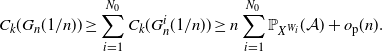 \begin{align*} C_k(G_n({1}/{n})) \geq \sum_{i=1}^{N_0} C_k(G^i_n({1}/{n})) \geq n\sum_{i=1}^{N_0} \mathbb{P}_{X^{W_i}}(\mathcal{A}) + o_\mathrm{p}(n).\end{align*}
Letting $N_0 \to N$
, we can conclude the proof for the lower bound. From now on, let us assume that W is irreducible.
$N_0 \to N$
, we can conclude the proof for the lower bound. From now on, let us assume that W is irreducible.
We say a graphon F is finitary if there exist finitely many disjoint intervals $I_{t_i}$
,
$I_{t_i}$
, $i=1, \dots, M$
, such that
$i=1, \dots, M$
, such that $\cup_{i=1}^M I_{t_i}=[0,1]$
and the restriction of F on
$\cup_{i=1}^M I_{t_i}=[0,1]$
and the restriction of F on $I_{t_i} \times I_{t_j}$
is a constant for any
$I_{t_i} \times I_{t_j}$
is a constant for any $1 \leq i, j \leq M$
. As we will see, the indexes
$1 \leq i, j \leq M$
. As we will see, the indexes $t_1,\dots,t_M$
will be used to label vertices of
$t_1,\dots,t_M$
will be used to label vertices of $G_n$
as well as particles of
$G_n$
as well as particles of $X^n$
. According to [Reference Bollobás, Janson and Riordan7, Lemma 7.3], the graphon W can be approximated pointwise from below by finitary graphons. More precisely, we have the following result.
$X^n$
. According to [Reference Bollobás, Janson and Riordan7, Lemma 7.3], the graphon W can be approximated pointwise from below by finitary graphons. More precisely, we have the following result.
Lemma 4.1. There exists a sequence of finitary graphons $(F_m)_{m\in\mathbb{N}}$
such that
$(F_m)_{m\in\mathbb{N}}$
such that $F_m \leq W$
and
$F_m \leq W$
and $\lim_{m\to\infty}F_m(x,y)=W(x,y)$
almost surely.
$\lim_{m\to\infty}F_m(x,y)=W(x,y)$
almost surely.
Under Assumption 2.1, we prove in Section 4.1 that, for any $\varepsilon>0$
,
$\varepsilon>0$
, $m \in \mathbb{N}$
,
$m \in \mathbb{N}$
,
 \begin{equation} C_k(G_n({1}/{n})) \geq (1-2\varepsilon)n\mathbb{P}_{X^{(1-2\varepsilon)F_m}}(\mathcal{A}) + o_\mathrm{p}(n).\end{equation}
Then, in Section 4.2, we show the continuity property
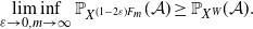 \begin{equation} \liminf_{\varepsilon\to0,m\to\infty}\mathbb{P}_{X^{(1-2\varepsilon)F_m}}(\mathcal{A}) \geq \mathbb{P}_{X^W}(\mathcal{A}).\end{equation}
It is clear that (4.1) and (4.2) together prove the lower bound part of Theorem 2.1, i.e. $C_k(G_n({1}/{n})) \geq n \mathbb{P}_{X^W}(\mathcal{A}) + o_\mathrm{p}(n)$
.
$C_k(G_n({1}/{n})) \geq n \mathbb{P}_{X^W}(\mathcal{A}) + o_\mathrm{p}(n)$
.
4.1. Proof of (4.1)
Fix $m \in \mathbb{N}$
and
$m \in \mathbb{N}$
and $\varepsilon \in (0,{1}/{m})$
such that
$\varepsilon \in (0,{1}/{m})$
such that $\lambda \to \mathbb{P}_{X^{\lambda (1-\varepsilon)F_m}}(\mathcal{A})$
is continuous at
$\lambda \to \mathbb{P}_{X^{\lambda (1-\varepsilon)F_m}}(\mathcal{A})$
is continuous at $\lambda =1$
. Since
$\lambda =1$
. Since $F_m$
is finitary, there exists a partition
$F_m$
is finitary, there exists a partition $I_{t_j},j=1,\dots, M$
of [0,1] such that
$I_{t_j},j=1,\dots, M$
of [0,1] such that $F_m|_{I_{t_j} \times I_{t_k}}$
is a constant denoted by
$F_m|_{I_{t_j} \times I_{t_k}}$
is a constant denoted by $F_m(t_j,t_k)$
. We will mark particles of the branching process
$F_m(t_j,t_k)$
. We will mark particles of the branching process $X^{G_n}$
by labels
$X^{G_n}$
by labels $t_h$
,
$t_h$
, $h=1,\dots,M$
.
$h=1,\dots,M$
.
Before proceeding to the rigorous proof, let us first give the main ideas of our argument. For each $G_n$
, we prove there exist M disjoint subsets
$G_n$
, we prove there exist M disjoint subsets $\mathbf{Good}_{n, t_1},\dots, \mathbf{Good}_{n, t_M}$
of vertices such that, for any vertex
$\mathbf{Good}_{n, t_1},\dots, \mathbf{Good}_{n, t_M}$
of vertices such that, for any vertex $i \in \mathbf{Good}_{n, t_h}$
and
$i \in \mathbf{Good}_{n, t_h}$
and $k=1,\dots, M$
,
$k=1,\dots, M$
,
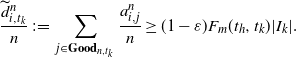 \begin{equation*} \frac{\widetilde{d}^n_{i,t_k}}{n} \,:\!=\, \sum_{j\in\mathbf{Good}_{n,t_k}}\frac{a^n_{i,j}}{n} \geq (1-\varepsilon)F_m(t_h,t_k)|I_k|.\end{equation*}
Therefore, we can heuristically consider $G_n$
as a ‘finitary’ graph by labelling vertices in
$G_n$
as a ‘finitary’ graph by labelling vertices in $\mathbf{Good}_{n,t_h}$
by
$\mathbf{Good}_{n,t_h}$
by $t_h$
,
$t_h$
, $h=1,\dots, M$
. Due to the above inequality, the branching process
$h=1,\dots, M$
. Due to the above inequality, the branching process $X^{G_n}$
associated with
$X^{G_n}$
associated with $G_n$
stochastically dominates, in the first order, the branching process
$G_n$
stochastically dominates, in the first order, the branching process $X^{(1-\varepsilon)F_m}$
associated with
$X^{(1-\varepsilon)F_m}$
associated with $(1-\varepsilon)F_m$
. Take
$(1-\varepsilon)F_m$
. Take $F^{\varepsilon}_m({1}/{n})$
to be an n-vertex random graph sampled from
$F^{\varepsilon}_m({1}/{n})$
to be an n-vertex random graph sampled from $(1-\varepsilon)F_m$
, i.e. independently uniformly select vertices
$(1-\varepsilon)F_m$
, i.e. independently uniformly select vertices $v_i \in [0,1]$
and then connect
$v_i \in [0,1]$
and then connect $v_i,v_j$
independently with probability
$v_i,v_j$
independently with probability $(1-\varepsilon)F_m(v_i,v_j)/n$
. By the standard exploration argument (see, e.g., [Reference Bollobás, Janson and Riordan7, Section 9]), locally the random graph
$(1-\varepsilon)F_m(v_i,v_j)/n$
. By the standard exploration argument (see, e.g., [Reference Bollobás, Janson and Riordan7, Section 9]), locally the random graph $G_n({1}/{n})$
(respectively
$G_n({1}/{n})$
(respectively $F^{\varepsilon}_m({1}/{n})$
) is almost the branching process
$F^{\varepsilon}_m({1}/{n})$
) is almost the branching process $X^{G_n}$
(respectively
$X^{G_n}$
(respectively $X^{(1-\varepsilon)F_m}$
). Thus, heuristically the random graph
$X^{(1-\varepsilon)F_m}$
). Thus, heuristically the random graph $G_n({1}/{n})$
is more connected than the random graph
$G_n({1}/{n})$
is more connected than the random graph $F^{\varepsilon}_m({1}/{n})$
, and thus has a k-core of larger order. Therefore, the inequality (4.1) follows from [Reference Riordan31, Theorem 3.1], which says that
$F^{\varepsilon}_m({1}/{n})$
, and thus has a k-core of larger order. Therefore, the inequality (4.1) follows from [Reference Riordan31, Theorem 3.1], which says that
 \begin{align*}C_k(F^{\varepsilon}_m({1}/{n})) = n \mathbb{P}_{X^{(1-\varepsilon)F_m}}(\mathcal{A})+o_\mathrm{p}(n).\end{align*}
The following simple lemma will be used to label vertices of $G_n$
. Therein, a vertex is defined to be ‘
$G_n$
. Therein, a vertex is defined to be ‘ $\mathbf{Bad}$
’ if its degree is not bounded from below by that of
$\mathbf{Bad}$
’ if its degree is not bounded from below by that of $F_m$
, and ‘
$F_m$
, and ‘ $\mathbf{Good}$
’ vertices are the complement of ‘
$\mathbf{Good}$
’ vertices are the complement of ‘ $\mathbf{Bad}$
’ ones.
$\mathbf{Bad}$
’ ones.
Lemma 4.2. Suppose $\varepsilon>0$
is a fixed constant, and
$\varepsilon>0$
is a fixed constant, and $\|W_{G_n}-W\|_{\square} \to 0$
. Then there exists a collection of disjoint subsets
$\|W_{G_n}-W\|_{\square} \to 0$
. Then there exists a collection of disjoint subsets $\widetilde{\mathbf{Bad}}_{n,t_j} \subset I_{t_j}$
,
$\widetilde{\mathbf{Bad}}_{n,t_j} \subset I_{t_j}$
, $j=1,\dots, M$
, such that [(i)]
$j=1,\dots, M$
, such that [(i)]
-
(i)
$|\widetilde{\mathbf{Bad}}_{n,t_j}| = o(1)$
,
$j=1,\dots, M$
; -
(ii) for any
$x \in I_{t_j} \setminus \widetilde{\mathbf{Bad}}_{n,t_j}$
, (4.3)
\begin{equation} \int_{I_{t_k}} W_{G_n}(x, y)\,\mathrm{d} y \geq (1-\varepsilon/2)F_m(t_j,t_k)|I_{t_k}|, \qquad k=1,\dots, M. \end{equation}


Proof. First, recall that we can also write
 \begin{equation} \|W\|_\square = \sup_{0\leq f,g \leq1 \text{ measurable}}\bigg|\int f(x)g(y)W(x,y)\,\mathrm{d} x\,\mathrm{d} y\bigg|. \end{equation}
For any $1 \leq j,k \leq M$
, define
$1 \leq j,k \leq M$
, define
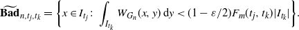 \begin{equation*} \widetilde{\mathbf{Bad}}_{n,t_j,t_k} = \bigg\{x\in I_{t_j}\colon \int_{I_{t_k}}W_{G_n}(x,y)\,\mathrm{d} y < (1-\varepsilon/2) F_m(t_j,t_k) |I_{t_k}| \bigg\}. \end{equation*}
In the case that $F_m(t_j,t_k) =0$
, it is clear that
$F_m(t_j,t_k) =0$
, it is clear that $\widetilde{\mathbf{Bad}}_{n,t_j,t_k}= \emptyset$
. Let us assume that
$\widetilde{\mathbf{Bad}}_{n,t_j,t_k}= \emptyset$
. Let us assume that $F_m(t_j,t_k)>0$
.
$F_m(t_j,t_k)>0$
.
Taking $f(x)=\mathbf{1}_{\{x\in\widetilde{\mathbf{Bad}}_{n,t_j,t_k}\}}$
and
$f(x)=\mathbf{1}_{\{x\in\widetilde{\mathbf{Bad}}_{n,t_j,t_k}\}}$
and $g(y)=\mathbf{1}_{\{y\in I_{t_k}\}}$
in (4.4), we obtain
$g(y)=\mathbf{1}_{\{y\in I_{t_k}\}}$
in (4.4), we obtain
 \begin{equation*} \int_{\widetilde{\mathbf{Bad}}_{n,t_j,t_k}}\mathrm{d} x\int_{I_{t_k}}(W_{G_n}(x,y)-W(x,y))\,\mathrm{d} y \geq -\|W_{G_n}-W\|_{\square} = -o(1), \end{equation*}
and, since $F_m \leq W$
,
$F_m \leq W$
,
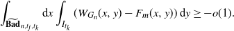 \begin{equation} \int_{\widetilde{\mathbf{Bad}}_{n,t_j,t_k}}\mathrm{d} x\int_{I_{t_k}}(W_{G_n}(x,y)-F_m(x,y))\,\mathrm{d} y \geq -o(1). \end{equation}
Since, for any $x\in\widetilde{\mathbf{Bad}}_{n,t_j,t_k}$
,
$x\in\widetilde{\mathbf{Bad}}_{n,t_j,t_k}$
,
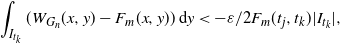 \begin{align*}\int_{I_{t_k}}(W_{G_n}(x,y)-F_m(x,y))\,\mathrm{d} y < -\varepsilon/2 F_m(t_j,t_k) |I_{t_k}|,\end{align*}
together with (4.5) it follows that $\varepsilon F_m(t_j,t_k)|I_{t_k}|\, |\widetilde{\mathbf{Bad}}_{n,t_j,t_k}| \leq o(1)$
. As a result of
$\varepsilon F_m(t_j,t_k)|I_{t_k}|\, |\widetilde{\mathbf{Bad}}_{n,t_j,t_k}| \leq o(1)$
. As a result of $F_m(t_j,t_k)>0$
, we obtain
$F_m(t_j,t_k)>0$
, we obtain $|\widetilde{\mathbf{Bad}}_{n,t_j,t_k}| = o(1)$
.
$|\widetilde{\mathbf{Bad}}_{n,t_j,t_k}| = o(1)$
.
If we take $\widetilde{\mathbf{Bad}}_{n,t_j}=\bigcup_{k=1}^M\widetilde{\mathbf{Bad}}_{n,t_j,t_k}$
, it is clear that
$\widetilde{\mathbf{Bad}}_{n,t_j}=\bigcup_{k=1}^M\widetilde{\mathbf{Bad}}_{n,t_j,t_k}$
, it is clear that $|\widetilde{\mathbf{Bad}}_{n, t_j}| = o(1)$
and satisfies (4.3).
$|\widetilde{\mathbf{Bad}}_{n, t_j}| = o(1)$
and satisfies (4.3).
Before proving the main result in this subsection, we would like to point out that our main contribution here is the observation that we can label vertices of $G_n$
so that heuristically it dominates the finitary graphon
$G_n$
so that heuristically it dominates the finitary graphon $(1-\varepsilon)F_m$
. The remaining part of the proof is just a modification of [Reference Riordan31, Theorem 3.1]. We summarize it as the following lemma, and refer the reader to [Reference Riordan31] for a detailed argument.
$(1-\varepsilon)F_m$
. The remaining part of the proof is just a modification of [Reference Riordan31, Theorem 3.1]. We summarize it as the following lemma, and refer the reader to [Reference Riordan31] for a detailed argument.
Lemma 4.3. Suppose $F_m$
is a finitary graphon with M labels
$F_m$
is a finitary graphon with M labels $t_1,\dots,t_M$
, and
$t_1,\dots,t_M$
, and $\lambda\to\mathbb{P}_{X^{\lambda F_m}}(\mathcal{A})$
is continuous at
$\lambda\to\mathbb{P}_{X^{\lambda F_m}}(\mathcal{A})$
is continuous at $\lambda=1$
. Let
$\lambda=1$
. Let $G_n$
be a sequence of graphs such that
$G_n$
be a sequence of graphs such that $\sup_{i,j,n}\{a^n_{i,j}\} < +\infty$
. Denote by
$\sup_{i,j,n}\{a^n_{i,j}\} < +\infty$
. Denote by $X^{G_n}_i$
(respectively
$X^{G_n}_i$
(respectively $X^{F_m}_{t_h}$
) the branching process associated with
$X^{F_m}_{t_h}$
) the branching process associated with $G_n$
(respectively
$G_n$
(respectively $F_m$
) that has the initial particle with type i (respectively label
$F_m$
) that has the initial particle with type i (respectively label $t_h$
). If, for each
$t_h$
). If, for each $G_n$
, there exist M disjoint subsets
$G_n$
, there exist M disjoint subsets $\mathbf{G}_{n,t_h}$
,
$\mathbf{G}_{n,t_h}$
, $h=1,\dots,M$
, of vertices such that, for some
$h=1,\dots,M$
, of vertices such that, for some $\varepsilon \in (0,1)$
,
$\varepsilon \in (0,1)$
,
-
(i)
${|\mathbf{G}_{n,t_h}|}/{n} \geq (1-\varepsilon)|I_{t_h}|$
,
$h=1,\dots,M$
; -
(ii) for each vertex
$i\in\mathbf{G}_{n,t_h}$
, the branching process
$X^{G_n}_{i}$
stochastically dominates, in the first order, the branching process
$X^{F_m}_{t_h}$
, then
$C_k(G_n({1}/{n})) \geq (1-\varepsilon)n\mathbb{P}_{X^{(1-\varepsilon)F_m}}(\mathcal{A}) + o_\mathrm{p}(n)$
.


Completing the proof of (4.1). Since $\lambda\to\mathbb{P}_{X^{\lambda F_m}}(\mathcal{A})$
is non-decreasing with respect to
$\lambda\to\mathbb{P}_{X^{\lambda F_m}}(\mathcal{A})$
is non-decreasing with respect to $\lambda$
, it has only countably many discontinuity points. Therefore, we can choose an arbitrarily small
$\lambda$
, it has only countably many discontinuity points. Therefore, we can choose an arbitrarily small $\varepsilon$
such that
$\varepsilon$
such that $\lambda\to\mathbb{P}_{X^{\lambda(1-\varepsilon)F_m}}(\mathcal{A})$
is continuous at
$\lambda\to\mathbb{P}_{X^{\lambda(1-\varepsilon)F_m}}(\mathcal{A})$
is continuous at $\lambda=1$
. We choose
$\lambda=1$
. We choose $0<\varepsilon<{1}/{m}$
, and take
$0<\varepsilon<{1}/{m}$
, and take $\widetilde{\mathbf{Bad}}_{n,t_h}$
as in Lemma 4.2. For
$\widetilde{\mathbf{Bad}}_{n,t_h}$
as in Lemma 4.2. For $h=1,\dots,M$
, define
$h=1,\dots,M$
, define
 \begin{equation*} \mathbf{Good}_{n,t_h} \,:\!=\, \{i\in[n]\colon(({i-1})/{n},{i}/{n}] \subset I_{t_h} \setminus \widetilde{\mathbf{Bad}}_{n,t_h}\}. \end{equation*}
Due to the construction of $W_{G_n}$
in (2.1), for any
$W_{G_n}$
in (2.1), for any $(({i-1})/{n},{i}/{n}] \subset I_{t_h}$
, we have either
$(({i-1})/{n},{i}/{n}] \subset I_{t_h}$
, we have either $(({i-1})/{n},{i}/{n}] \subset \widetilde{\mathbf{Bad}}_{n,t_h}$
or
$(({i-1})/{n},{i}/{n}] \subset \widetilde{\mathbf{Bad}}_{n,t_h}$
or $(({i-1})/{n},{i}/{n}] \cap \widetilde{\mathbf{Bad}}_{n,t_h}=\emptyset$
. Therefore, it can be easily verified that
$(({i-1})/{n},{i}/{n}] \cap \widetilde{\mathbf{Bad}}_{n,t_h}=\emptyset$
. Therefore, it can be easily verified that ${|\mathbf{Good}_{n,t_h}|}/{n} \geq |I_{t_h}| - o(1)$
. For any
${|\mathbf{Good}_{n,t_h}|}/{n} \geq |I_{t_h}| - o(1)$
. For any $i\in\mathbf{Good}_{n,t_h}$
, define
$i\in\mathbf{Good}_{n,t_h}$
, define $\widetilde{d}^n_{i,t_k}\,:\!=\,\sum_{j\in\mathbf{Good}_{n,t_k}}a^n_{i,j}$
,
$\widetilde{d}^n_{i,t_k}\,:\!=\,\sum_{j\in\mathbf{Good}_{n,t_k}}a^n_{i,j}$
, $k=1,\dots,M$
. As a result of (4.3), we obtain
$k=1,\dots,M$
. As a result of (4.3), we obtain
 \begin{equation*} \frac{\widetilde{d}^n_{i,t_k}}{n} \geq \int_{I_{t_k}}W_{G_n}(i/n,y)\,\mathrm{d} y - \bar{a}(|I_{t_k}|-{|\mathbf{Good}_{n,t_k}|}/{n}) \geq (1-\varepsilon/2)F_m(t_h,t_k)|I_{t_k}| - o(1)\bar{a}. \end{equation*}
We conclude that, for large enough n, there exists a collection of disjoint $\mathbf{Good}_{n,t_h} \subset [n]$
,
$\mathbf{Good}_{n,t_h} \subset [n]$
, $h=1,\dots,M$
, which satisfies the following:
$h=1,\dots,M$
, which satisfies the following:
-
(i) For all
$h=1,\dots,M$
, (4.6)
\begin{equation} {|\mathbf{Good}_{n,t_h}|}/{n} \geq (1- \varepsilon)|I_{t_h}|. \end{equation}
-
(ii) For any
$i\in\mathbf{Good}_{n,t_h}$
, (4.7)
\begin{equation} \frac{\widetilde{d}^n_{i,t_k}}{n} \geq (1-\varepsilon) F_m(t_h,t_k)|I_{t_k}|, \quad k=1,\dots, M. \end{equation}


For vertices in $\mathbf{Good}_{n,t_h}$
,
$\mathbf{Good}_{n,t_h}$
, $h=1,\dots,M$
, we label them with
$h=1,\dots,M$
, we label them with $t_h$
. Let us define
$t_h$
. Let us define $\mathbf{Good}_{n}\,:\!=\,\bigcup_{h=1}^M\mathbf{Good}_{n,t_h}$
,
$\mathbf{Good}_{n}\,:\!=\,\bigcup_{h=1}^M\mathbf{Good}_{n,t_h}$
, $\tilde{n}\,:\!=\,|\mathbf{Good}_{n}|$
. Let
$\tilde{n}\,:\!=\,|\mathbf{Good}_{n}|$
. Let $\widetilde{G}_{\tilde{n}}$
be the graph with vertices
$\widetilde{G}_{\tilde{n}}$
be the graph with vertices $\mathbf{Good}_n$
such that
$\mathbf{Good}_n$
such that $\widetilde{a}^n_{i,j}\,:\!=\,\tilde{n}a^n_{i,j}/n$
for all
$\widetilde{a}^n_{i,j}\,:\!=\,\tilde{n}a^n_{i,j}/n$
for all $i,j \in \mathbf{Good}_n$
. It is clear that
$i,j \in \mathbf{Good}_n$
. It is clear that $C_k(G_n({1}/{n})) \geq C_k(\widetilde{G}_{\tilde{n}}({1}/{\tilde{n}}))$
.
$C_k(G_n({1}/{n})) \geq C_k(\widetilde{G}_{\tilde{n}}({1}/{\tilde{n}}))$
.
Take $\widetilde{X}^{\tilde{n}}$
to be a branching process sampled from
$\widetilde{X}^{\tilde{n}}$
to be a branching process sampled from $\widetilde{G}_{\tilde{n}}$
. For any
$\widetilde{G}_{\tilde{n}}$
. For any $i \in \mathbf{Good}_{n,t_h}$
, take
$i \in \mathbf{Good}_{n,t_h}$
, take $\widetilde{X}^{\tilde{n}}_i$
to be a branching process sampled from graph
$\widetilde{X}^{\tilde{n}}_i$
to be a branching process sampled from graph $\widetilde{G}_{\tilde{n}}$
with root i. For any
$\widetilde{G}_{\tilde{n}}$
with root i. For any $t_h$
, take
$t_h$
, take $X^{(1-\varepsilon)F_m}_{t_h}$
to be a branching process sampled from graphon
$X^{(1-\varepsilon)F_m}_{t_h}$
to be a branching process sampled from graphon $(1-\varepsilon)F_m$
with root of label
$(1-\varepsilon)F_m$
with root of label $t_h$
. Suppose a particle in generation t of
$t_h$
. Suppose a particle in generation t of $\widetilde{X}_i^{\tilde{n}}$
is of type j with label
$\widetilde{X}_i^{\tilde{n}}$
is of type j with label $t_h$
. As a result of (4.7) the number of its
$t_h$
. As a result of (4.7) the number of its $t_k$
-labelled children has Poisson distribution with parameter
$t_k$
-labelled children has Poisson distribution with parameter $\widetilde{d}^n_{j,t_k}/n$
, which is larger than
$\widetilde{d}^n_{j,t_k}/n$
, which is larger than $(1-\varepsilon) F_m(t_h,t_k)|I_{t_k}|$
. Therefore, for any
$(1-\varepsilon) F_m(t_h,t_k)|I_{t_k}|$
. Therefore, for any $i \in \mathbf{Good}_{n,t_h}$
, we can consider
$i \in \mathbf{Good}_{n,t_h}$
, we can consider $X^{(1-\varepsilon)F_m}_{t_h}$
as a subset of
$X^{(1-\varepsilon)F_m}_{t_h}$
as a subset of $\widetilde{X}_i^{\tilde{n}}$
. Thus, for any increasing event
$\widetilde{X}_i^{\tilde{n}}$
. Thus, for any increasing event $\mathcal{I}$
, we have
$\mathcal{I}$
, we have $\mathbb{P}_{\widetilde{X}_i^{\tilde{n}}}(\mathcal{I}) \geq \mathbb{P}_{X^{(1-\varepsilon)F_m}_{t_h}}(\mathcal{I})$
.
$\mathbb{P}_{\widetilde{X}_i^{\tilde{n}}}(\mathcal{I}) \geq \mathbb{P}_{X^{(1-\varepsilon)F_m}_{t_h}}(\mathcal{I})$
.
Now we apply Lemma 4.3 to $(1-\varepsilon)F_m$
and
$(1-\varepsilon)F_m$
and $\widetilde{G}_{\tilde{n}}$
to conclude that
$\widetilde{G}_{\tilde{n}}$
to conclude that
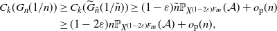 \begin{align*} C_k(G_n({1}/{n})) & \geq C_k(\widetilde{G}_{\tilde{n}}({1}/{\tilde{n}})) \geq (1-\varepsilon)\tilde{n}\mathbb{P}_{X^{(1-2\varepsilon)F_m}}(\mathcal{A})+o_\mathrm{p}(n) \\ & \geq (1-2\varepsilon) n \mathbb{P}_{X^{(1-2\varepsilon)F_m}}(\mathcal{A})+o_\mathrm{p}(n), \end{align*}
where in the last inequality we used the fact that $\tilde{n}/n \geq 1- \varepsilon$
due to (4.6).
$\tilde{n}/n \geq 1- \varepsilon$
due to (4.6).
4.2. Proof of (4.2)
Note that if $F_m$
converges to W pointwise from below, by the dominated convergence theorem it can be easily seen that
$F_m$
converges to W pointwise from below, by the dominated convergence theorem it can be easily seen that $\lim_{\varepsilon \to 0, m \to \infty} d_{\square}((1-2\varepsilon)F_m, W)=0$
. It is therefore sufficient to show that
$\lim_{\varepsilon \to 0, m \to \infty} d_{\square}((1-2\varepsilon)F_m, W)=0$
. It is therefore sufficient to show that $\lim_{n\to\infty}\mathbb{P}_{X^{W_n}}(\mathcal{A}) \geq \mathbb{P}_{X^W}(\mathcal{A})$
if
$\lim_{n\to\infty}\mathbb{P}_{X^{W_n}}(\mathcal{A}) \geq \mathbb{P}_{X^W}(\mathcal{A})$
if $\lim_{n\to\infty}d_{\square}(W_n,W)=0$
, which we prove in Proposition 4.1.
$\lim_{n\to\infty}d_{\square}(W_n,W)=0$
, which we prove in Proposition 4.1.
We say a branching process has property $\mathcal{B}_d$
if its root has at least
$\mathcal{B}_d$
if its root has at least $k-1$
children, each of these
$k-1$
children, each of these $k-1$
children has at least
$k-1$
children has at least $k-1$
children, and this occurs up to generation d, and let
$k-1$
children, and this occurs up to generation d, and let $\mathcal{B}=\cap_{d=1}^{\infty} \mathcal{B}_d$
. Define the function
$\mathcal{B}=\cap_{d=1}^{\infty} \mathcal{B}_d$
. Define the function $\mathbb{P}si_{k}(\lambda)\,:\!=\, \mathbb{P}( \text{Poi}(\lambda) \geq k)$
. For any graphon W, define
$\mathbb{P}si_{k}(\lambda)\,:\!=\, \mathbb{P}( \text{Poi}(\lambda) \geq k)$
. For any graphon W, define
 \begin{equation}\beta_{W} (x,d)\,:\!=\, \mathbb{P}\big( X^W \in \mathcal{B}_d \mid X^W_0=x \big), \qquad\beta_W(x)\,:\!=\, \mathbb{P}\big(X^W \in \mathcal{B} \mid X^W_0=x\big),\end{equation}
where $X^W_0$
stands for the type of the root. For
$X^W_0$
stands for the type of the root. For $W=W_n$
, we simply write
$W=W_n$
, we simply write $\beta_n(x,d)\,:\!=\,\beta_{W_n}(x,d)$
,
$\beta_n(x,d)\,:\!=\,\beta_{W_n}(x,d)$
, $\beta_n(x)\,:\!=\,\beta_{W_n}(x)$
.
$\beta_n(x)\,:\!=\,\beta_{W_n}(x)$
.
Lemma 4.4. Let $(W_n)_{n\in\mathbb{N}}$
be a sequence of graphons such that
$(W_n)_{n\in\mathbb{N}}$
be a sequence of graphons such that $\|W_n-W\|_\square \to 0$
. Suppose that W is irreducible, and
$\|W_n-W\|_\square \to 0$
. Suppose that W is irreducible, and $\alpha\colon[0,1]\rightarrow[0,1]$
is a strictly positive measurable function, i.e.
$\alpha\colon[0,1]\rightarrow[0,1]$
is a strictly positive measurable function, i.e. $\mathrm{Leb}(\{x\colon\alpha(x)>0\})=1$
. Fix
$\mathrm{Leb}(\{x\colon\alpha(x)>0\})=1$
. Fix $\varepsilon>0$
and
$\varepsilon>0$
and $\delta>0$
. Define a subset
$\delta>0$
. Define a subset $\mathbf{Bad}_n \subset [0,1]$
via
$\mathbf{Bad}_n \subset [0,1]$
via
 \begin{equation*} \mathbf{Bad}_nv\,:\!=\, \bigg\{x\colon(1-\varepsilon/2)\int\alpha(y)W(x,y)\,\mathrm{d} y > \int\alpha(y)W_n(x,y)\,\mathrm{d} y\bigg\}. \end{equation*}
Then $\mathrm{Leb}(\mathbf{Bad}_n) \leq \delta$
for large enough n.
$\mathrm{Leb}(\mathbf{Bad}_n) \leq \delta$
for large enough n.
Proof. According to the definition of the cut norm (4.4),
 \begin{equation*} \lVert W-W_n\rVert_{\square} \geq \int_{\mathbf{Bad}_n}\mathrm{d} x\int\alpha(y)(W(x,y)-W_n(x,y))\,\mathrm{d} y \geq \frac{\varepsilon}{2}\int_{\mathbf{Bad}_n}\,\mathrm{d} x\int\alpha(y)W(x,y)\,\mathrm{d} y. \end{equation*}
Note that $\widetilde{W}(x,y)=\alpha(x)\alpha(y)W(x,y)$
is still irreducible, and
$\widetilde{W}(x,y)=\alpha(x)\alpha(y)W(x,y)$
is still irreducible, and
 \begin{equation*} \lVert W-W_n\rVert_{\square} \geq \frac{\varepsilon}{2}\int_{\mathbf{Bad}_n}\mathrm{d} x \int\alpha(y)W(x,y)\,\mathrm{d} y \geq \frac{\varepsilon}{2}\int_{\mathbf{Bad}_n}\mathrm{d} x\int\widetilde{W}(x,y)\,\mathrm{d} y. \end{equation*}
Applying [Reference Bollobás, Borgs, Chayes and Riordan6, Lemma 7] to the irreducible $\widetilde{W}$
, we get that, given any
$\widetilde{W}$
, we get that, given any $\delta \in \big(0,\frac12\big)$
, there exists a positive number
$\delta \in \big(0,\frac12\big)$
, there exists a positive number $b(\widetilde{W},\delta)>0$
such that, for any
$b(\widetilde{W},\delta)>0$
such that, for any $A \subset [0,1]$
with
$A \subset [0,1]$
with $\delta \leq \mathrm{Leb}(A) \leq 1-\delta$
,
$\delta \leq \mathrm{Leb}(A) \leq 1-\delta$
, $\int_{A\times A^\mathrm{c}}\widetilde{W}(x,y)\,\mathrm{d} x\,\mathrm{d} y>b$
. Now, since
$\int_{A\times A^\mathrm{c}}\widetilde{W}(x,y)\,\mathrm{d} x\,\mathrm{d} y>b$
. Now, since
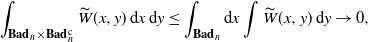 \begin{align*}\int_{\mathbf{Bad}_n\times\mathbf{Bad}_n^\mathrm{c}}\widetilde{W}(x,y)\,\mathrm{d} x\,\mathrm{d} y \leq \int_{\mathbf{Bad}_n}\mathrm{d} x\int\widetilde{W}(x,y)\,\mathrm{d} y \to 0,\end{align*}
we conclude that $\mathrm{Leb}(\mathbf{Bad}_n) \leq \delta$
for large enough n.
$\mathrm{Leb}(\mathbf{Bad}_n) \leq \delta$
for large enough n.
Lemma 4.5. Let $k \in \mathbb{N}$
, and W be an irreducible graphon such that
$k \in \mathbb{N}$
, and W be an irreducible graphon such that
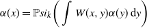 \begin{align} \alpha(x) = \mathbb{P}si_k\bigg(\int W(x,y)\alpha(y)\,\mathrm{d} y\bigg) \end{align}
has a solution $\alpha(x)$
with
$\alpha(x)$
with $\mathrm{Leb}(\{x\colon\alpha(x)=0\})<1$
. Then
$\mathrm{Leb}(\{x\colon\alpha(x)=0\})<1$
. Then $\alpha$
is strictly positive, i.e.
$\alpha$
is strictly positive, i.e. $\mathrm{Leb}(\{x\colon\alpha(x)>0\})=1$
.
$\mathrm{Leb}(\{x\colon\alpha(x)>0\})=1$
.
Proof. Suppose $\alpha$
is a non-zero solution of (4.9). Define
$\alpha$
is a non-zero solution of (4.9). Define $\mathcal{Z}\,:\!=\,\{x\colon\alpha(x)=0\}$
. For any
$\mathcal{Z}\,:\!=\,\{x\colon\alpha(x)=0\}$
. For any $x \in \mathcal{Z}$
,
$x \in \mathcal{Z}$
, $0 = \mathbb{P}si_k\big(\int W(x,y)\alpha(y)\,\mathrm{d} y\big)$
, which can only happen if
$0 = \mathbb{P}si_k\big(\int W(x,y)\alpha(y)\,\mathrm{d} y\big)$
, which can only happen if $\int_{\mathcal{Z}^\mathrm{c}}W(x,y)\alpha(y)\,\mathrm{d} y = 0$
. Integrating this equation over
$\int_{\mathcal{Z}^\mathrm{c}}W(x,y)\alpha(y)\,\mathrm{d} y = 0$
. Integrating this equation over $x \in \mathcal{Z}$
, we obtain
$x \in \mathcal{Z}$
, we obtain
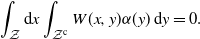 \begin{equation*} \int_{\mathcal{Z}}\mathrm{d} x\int_{\mathcal{Z}^\mathrm{c}}W(x,y)\alpha(y)\,\mathrm{d} y = 0. \end{equation*}
Since $\alpha>0$
over
$\alpha>0$
over $\mathcal{Z}^\mathrm{c}$
, this violates the irreducibility of W.
$\mathcal{Z}^\mathrm{c}$
, this violates the irreducibility of W.
Proposition 4.1. Let $(W_n)_{n\in\mathbb{N}}$
be a sequence of graphons such that
$(W_n)_{n\in\mathbb{N}}$
be a sequence of graphons such that $d_{\square}(W_n, W) \rightarrow 0$
with irreducible W. Then, for any
$d_{\square}(W_n, W) \rightarrow 0$
with irreducible W. Then, for any $\varepsilon>0$
,
$\varepsilon>0$
,
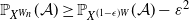 \begin{equation} \mathbb{P}_{X^{W_n}}(\mathcal{A}) \geq \mathbb{P}_{X^{(1-\epsilon)W}}(\mathcal{A})-\varepsilon^2 \end{equation}
for large enough n. Then, under Assumption 2.1, $\liminf_{n\to\infty}\mathbb{P}_{X^{W_n}}(\mathcal{A}) \geq \mathbb{P}_{X^W}(\mathcal{A})$
.
$\liminf_{n\to\infty}\mathbb{P}_{X^{W_n}}(\mathcal{A}) \geq \mathbb{P}_{X^W}(\mathcal{A})$
.
Proof. We will only prove (4.10), since the second statement follows directly from this. Assume there exists some $\varepsilon_0>0$
such that
$\varepsilon_0>0$
such that $\mathbb{P}_{X^{(1-\varepsilon_0) W}}(\mathcal{A})>0$
(otherwise, there is nothing to prove). Recalling the definition of
$\mathbb{P}_{X^{(1-\varepsilon_0) W}}(\mathcal{A})>0$
(otherwise, there is nothing to prove). Recalling the definition of $\beta_{(1-\varepsilon_0) W}(x) $
as in (4.8), we have the equality
$\beta_{(1-\varepsilon_0) W}(x) $
as in (4.8), we have the equality
 \begin{align*} \mathbb{P}_{X^{(1-\varepsilon_0)W}}(\mathcal{A}) = \int\mathbb{P}si_{k}\bigg(\int(1-\varepsilon_0)W(x,y)\beta_{(1-\varepsilon_0)W}(y)\,\mathrm{d} y\bigg)\,\mathrm{d} x, \end{align*}
and hence $\mathrm{Leb}\{x\colon\beta_{(1-\varepsilon_0)W}(x)>0\}>0$
. Since
$\mathrm{Leb}\{x\colon\beta_{(1-\varepsilon_0)W}(x)>0\}>0$
. Since $\beta_{(1-\varepsilon_0)W}(x)$
is a solution of
$\beta_{(1-\varepsilon_0)W}(x)$
is a solution of
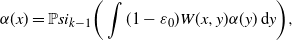 \begin{equation*} \alpha(x)=\mathbb{P}si_{k-1}\bigg(\int(1-\varepsilon_0)W(x,y)\alpha(y)\,\mathrm{d} y\bigg), \end{equation*} $\beta_{(1-\varepsilon_0)W}(x)$
is strictly positive according to Lemma 4.5. Fix any
$\beta_{(1-\varepsilon_0)W}(x)$
is strictly positive according to Lemma 4.5. Fix any $\varepsilon \in (0,\varepsilon_0)$
. We first prove the following statement by induction: for each
$\varepsilon \in (0,\varepsilon_0)$
. We first prove the following statement by induction: for each $d \geq 1$
and
$d \geq 1$
and $\delta >0$
, there exist subsets
$\delta >0$
, there exist subsets $\mathbf{Bad}_{n,d} \subset [0,1]$
for large enough n such that
$\mathbf{Bad}_{n,d} \subset [0,1]$
for large enough n such that $\mathrm{Leb}(\mathbf{Bad}_{n,d})< \delta$
and
$\mathrm{Leb}(\mathbf{Bad}_{n,d})< \delta$
and $\beta_n(x,d)\geq\beta_{(1-\varepsilon)W}(x,d)$
, for any
$\beta_n(x,d)\geq\beta_{(1-\varepsilon)W}(x,d)$
, for any $x \in \mathbf{Bad}^\mathrm{c}_{n,d}$
,
$x \in \mathbf{Bad}^\mathrm{c}_{n,d}$
, $d \geq 1$
.
$d \geq 1$
.
Applying Lemma 4.4 with $\alpha(y)=1$
, for all
$\alpha(y)=1$
, for all $y \in [0,1]$
, we obtain some
$y \in [0,1]$
, we obtain some $\mathbf{Bad}_{n,1}$
with
$\mathbf{Bad}_{n,1}$
with $\mathrm{Leb}(\mathbf{Bad}_{n,1}) \leq \delta$
such that
$\mathrm{Leb}(\mathbf{Bad}_{n,1}) \leq \delta$
such that $x\in\mathbf{Bad}_{n,1}^\mathrm{c}$
implies
$x\in\mathbf{Bad}_{n,1}^\mathrm{c}$
implies $\int W_n(x,y)\,\mathrm{d} y\geq(1-\varepsilon/2)\int W(x,y)\,\mathrm{d} y$
. It follows that
$\int W_n(x,y)\,\mathrm{d} y\geq(1-\varepsilon/2)\int W(x,y)\,\mathrm{d} y$
. It follows that
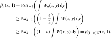 \begin{align*} \beta_n(x,1) & = \mathbb{P}si_{k-1}\bigg(\int W_n(x,y)\,\mathrm{d} y\bigg) \\ & \geq \mathbb{P}si_{k-1}\bigg(\bigg(1-\frac{\varepsilon}{2}\bigg)\int W(x,y)\,\mathrm{d} y\bigg) \\ & \geq \mathbb{P}si_{k-1}\bigg((1-\varepsilon)\int W(x,y)\,\mathrm{d} y\bigg) = \beta_{(1-\varepsilon)W}(x,1). \end{align*}
Assume our assertion holds for $d-1$
and
$d-1$
and $\delta'>0$
, where
$\delta'>0$
, where $\delta'$
is to be chosen later. Let us now prove our claim for d and
$\delta'$
is to be chosen later. Let us now prove our claim for d and $\delta>0$
. Noting that
$\delta>0$
. Noting that
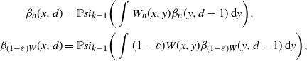 \begin{align*} \beta_n(x,d) & = \mathbb{P}si_{k-1}\bigg(\int W_n(x,y)\beta_n(y,d-1)\,\mathrm{d} y\bigg), \\ \beta_{(1-\varepsilon)W}(x,d) & = \mathbb{P}si_{k-1}\bigg(\int(1-\varepsilon)W(x,y)\beta_{(1-\varepsilon)W}(y,d-1)\,\mathrm{d} y\bigg), \end{align*}
it is enough to show there exists $\mathbf{Bad}_{n,d}$
such that
$\mathbf{Bad}_{n,d}$
such that $x\in\mathbf{Bad}_{n,d}^\mathrm{c}$
implies
$x\in\mathbf{Bad}_{n,d}^\mathrm{c}$
implies
 \begin{equation} \int W_n(x,y)\beta_n(y,d-1)\,\mathrm{d} y \geq \int(1-\varepsilon)W(x,y)\beta_{(1-\varepsilon)W}(y,d-1)\,\mathrm{d} y. \end{equation}
Applying Lemma 4.4 with $\alpha(y)=\beta_{(1-\varepsilon)W}(y,d-1)>0$
, we obtain, for large enough n, a subset
$\alpha(y)=\beta_{(1-\varepsilon)W}(y,d-1)>0$
, we obtain, for large enough n, a subset $\widetilde{\mathbf{Bad}}_{n,d}$
with
$\widetilde{\mathbf{Bad}}_{n,d}$
with $\mathrm{Leb}(\widetilde{\mathbf{Bad}}_{n,d}) \leq \delta/2$
such that
$\mathrm{Leb}(\widetilde{\mathbf{Bad}}_{n,d}) \leq \delta/2$
such that $x\in\widetilde{\mathbf{Bad}}^\mathrm{c}_{n,d}$
implies
$x\in\widetilde{\mathbf{Bad}}^\mathrm{c}_{n,d}$
implies
 \begin{equation*} \int W_n(x,y)\beta_{(1-{\varepsilon})W}(y,d-1)\,\mathrm{d} y \geq \bigg(1-\frac{\varepsilon}{2}\bigg)\int W(x,y)\beta_{(1-\varepsilon)W}(y,d-1)\,\mathrm{d} y. \end{equation*}
Since $\beta_{(1-\varepsilon)W}(x)$
is strictly positive,
$\beta_{(1-\varepsilon)W}(x)$
is strictly positive, $\lim_{\xi\searrow0}\mathrm{Leb}(\{x\colon\beta_{(1-\varepsilon)W}(x)\geq\xi\})=1$
. Therefore, there exists a subset
$\lim_{\xi\searrow0}\mathrm{Leb}(\{x\colon\beta_{(1-\varepsilon)W}(x)\geq\xi\})=1$
. Therefore, there exists a subset $\mathbf{Bad} \subset [0,1]$
and a positive constant
$\mathbf{Bad} \subset [0,1]$
and a positive constant $\xi$
such that
$\xi$
such that $\mathrm{Leb}(\mathbf{Bad}) \leq \delta/4$
and, for any
$\mathrm{Leb}(\mathbf{Bad}) \leq \delta/4$
and, for any $x \in \mathbf{Bad}^\mathrm{c}$
,
$x \in \mathbf{Bad}^\mathrm{c}$
,
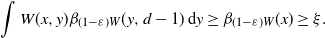 \begin{equation*} \int W(x,y)\beta_{(1-\varepsilon)W}(y,d-1)\,\mathrm{d} y \geq \beta_{(1-\varepsilon)W}(x) \geq \xi. \end{equation*}
By induction, it follows that, for $x\in\mathbf{Bad}_{n,d}^\mathrm{c} \,:\!=\, \mathbf{Bad}_{n,d-1}^\mathrm{c} \cap \widetilde{\mathbf{Bad}}_{n,d}^\mathrm{c} \cap \mathbf{Bad}^\mathrm{c}$
,
$x\in\mathbf{Bad}_{n,d}^\mathrm{c} \,:\!=\, \mathbf{Bad}_{n,d-1}^\mathrm{c} \cap \widetilde{\mathbf{Bad}}_{n,d}^\mathrm{c} \cap \mathbf{Bad}^\mathrm{c}$
,
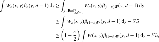 \begin{align*} \int W_n(x,y)\beta_n(y,d-1)\,\mathrm{d} y & \geq \int_{y\in\mathbf{Bad}_{n,d-1}^\mathrm{c}}W_n(x,y)\beta_{(1-{\varepsilon})W}(y,d-1)\,\mathrm{d} y \\ & \geq \int W_n(x,y)\beta_{(1-\varepsilon)W}(y,d-1)\,\mathrm{d} y - \delta'\bar{a} \\ & \geq \bigg(1-\frac{\varepsilon}{2}\bigg)\int W(x,y)\beta_{(1-\varepsilon)W}(y,d-1)\,\mathrm{d} y - \delta'\bar{a}, \end{align*}
where the first two inequalities are due to our induction hypothesis and the third inequality follows from our choice of $\widetilde{\mathbf{Bad}}_{n,d}$
. Choosing a small enough
$\widetilde{\mathbf{Bad}}_{n,d}$
. Choosing a small enough $\delta'\in(0,\delta/4)$
that
$\delta'\in(0,\delta/4)$
that $\delta'\bar{a} \leq {\varepsilon\xi}/{2}$
, it is clear that (4.11) holds for
$\delta'\bar{a} \leq {\varepsilon\xi}/{2}$
, it is clear that (4.11) holds for $x\in\mathbf{Bad}_{n,d}^\mathrm{c}$
with
$x\in\mathbf{Bad}_{n,d}^\mathrm{c}$
with $\mathrm{Leb}(\mathbf{Bad}_{n,d}) \leq \delta$
.
$\mathrm{Leb}(\mathbf{Bad}_{n,d}) \leq \delta$
.
Now we prove that $\mathbb{P}_{X^{W_n}}(\mathcal{A}) \geq \mathbb{P}_{X^{(1-\epsilon)W}}(\mathcal{A})-\varepsilon^2$
. Note that
$\mathbb{P}_{X^{W_n}}(\mathcal{A}) \geq \mathbb{P}_{X^{(1-\epsilon)W}}(\mathcal{A})-\varepsilon^2$
. Note that
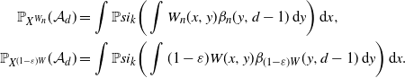 \begin{align*} \mathbb{P}_{X^{W_n}}(\mathcal{A}_d) & = \int\mathbb{P}si_k\bigg(\int W_n(x,y)\beta_n(y,d-1)\,\mathrm{d} y\bigg)\,\mathrm{d} x, \\ \mathbb{P}_{X^{(1-\varepsilon)W}}(\mathcal{A}_d) & = \int\mathbb{P}si_k\bigg(\int(1-\varepsilon)W(x,y)\beta_{(1-\varepsilon)W}(y,d-1)\,\mathrm{d} y\bigg)\,\mathrm{d} x. \end{align*}
Choosing $\delta =\varepsilon^2$
, there exists, for large enough n, a subset
$\delta =\varepsilon^2$
, there exists, for large enough n, a subset $\mathbf{Bad}_{n,d}$
with
$\mathbf{Bad}_{n,d}$
with $\mathrm{Leb}(\mathbf{Bad}_{n,d})\leq \delta$
such that
$\mathrm{Leb}(\mathbf{Bad}_{n,d})\leq \delta$
such that $x \in \mathbf{Bad}_{n,d}^\mathrm{c}$
implies
$x \in \mathbf{Bad}_{n,d}^\mathrm{c}$
implies
 \begin{equation*} \mathbb{P}si_k\bigg(\int W_n(x,y)\beta_n(y,d-1)\,\mathrm{d} y\bigg) \geq \mathbb{P}si_k\bigg(\int(1-\varepsilon)W(x,y)\beta_{(1-\varepsilon)W}(y,d-1)\,\mathrm{d} y\bigg). \end{equation*}
Since $\mathbb{P}si_k(x) \leq 1$
for all
$\mathbb{P}si_k(x) \leq 1$
for all $x \geq 0$
, it can be easily verified that
$x \geq 0$
, it can be easily verified that $\mathbb{P}_{X^{W_n}}(\mathcal{A}_d) \geq \mathbb{P}_{X^{(1-\varepsilon)W}}(\mathcal{A}_d)-\varepsilon^2$
. Letting
$\mathbb{P}_{X^{W_n}}(\mathcal{A}_d) \geq \mathbb{P}_{X^{(1-\varepsilon)W}}(\mathcal{A}_d)-\varepsilon^2$
. Letting $d \to \infty$
in this inequality, we conclude the result.
$d \to \infty$
in this inequality, we conclude the result.
Acknowledgements
We wish to thank Remco van der Hofstad for his comments connecting our work to the emergence of a giant k-core, which led to Remark 2.1.
Funding information
E. B. is partially supported by the National Science Foundation under grant DMS-2106556 and by the Susan M. Smith chair. S. C. is partially supported by the Netherlands Organisation for Scientific Research (NWO) through Gravitation-grant NETWORKS-024.002.003.
Competing interests
There were no competing interests to declare which arose during the preparation or publication process of this article.


 Open access