


1. Introduction
Heat-related fatalities are a significant component of mortality risks from climate change in the United States and globally. Climate change contributes to heat deaths by increasing the number of days each year in which temperatures and humidity are dangerously high, causing dehydration, heat stroke, and organ failure in individuals who are exposed to heat for too long (e.g., Dell et al., Reference Dell, Jones and Olken2014; Barreca et al., Reference Barreca, Clay, Deschenes, Greenstone and Shapiro2016; Chilton et al., Reference Chilton, Duxbury, Mussio, Nielsen and Sharma2024). Between 2021 and 2023, heat-related deaths in the United States increased by nearly 50% from 1,530 deaths to 2,262 (CDC, 2024). Such government reports of heat deaths may, in fact, undercount the mortality burden of heat because death certificates may undercount the number of deaths truly associated with excess heat (Green et al., Reference Green, Lysaght, Saulnier, Blanchard, Humphrey, Fakhruddin and Murray2019). Heat-related mortality risks are largest for seniors, with individuals older than 65 accounting for more than 40% of heat deaths between 2021 and 2023. Heat-related deaths to seniors comprise a prominent component of estimates of the social cost of greenhouse gases (U.S. EPA, 2023). Globally, heat is expected to kill approximately 92,000 seniors annually by 2030 and approximately 255,000 annually by 2050 if countries do not adapt to rising temperatures (WHO, 2014). The U.S. Environmental Protection Agency (EPA) (2021, 2023) uses heat-related deaths as a metric for monitoring the trend in the impact of global warming. Accordingly, reducing heat-related mortality risks, and determining the appropriate mortality risk benefit value to ascribe to such a risk reduction in benefit-cost analyses of relevant policies, is a regulatory analysis priority.
Although government agencies do not typically differentiate the monetized value of mortality risk reductions by cause of death or the age of decedents when they engage in benefit-cost analyses, previous research demonstrates that individuals place different values on mortality risks that involve varying degrees of morbidity. The canonical example of a mortality risk with a premium for the value of a statistical life (VSL) is cancer – several studies have found that individuals prefer to reduce cancer deaths more than deaths from other causes (e.g., Magat et al., Reference Magat, Viscusi and Huber1996; Van Houtven et al., Reference Van Houtven, Sullivan and Dockins2008; Viscusi et al., Reference Viscusi, Huber and Bell2014; Masterman & Viscusi, Reference Masterman and Viscusi2020). Even for traumatic injuries, individuals place a premium on fatality risks linked to significant long-term morbidity (Gentry & Viscusi, Reference Gentry and Viscusi2016). Individuals may also place a higher value on risk reductions from particularly vivid or dreadful causes, or those that are the subject of ongoing public policy debates, such as terrorism or mass shooting risks (Chilton et al., Reference Chilton, Jones-Lee, Kiraly, Metcalf and Pang2006; Dalafave & Viscusi, Reference Dalafave and Viscusi2021). Although there also could be additional altruistic components to valuations, people generally value reductions that benefit themselves or their family more than those that affect the public at large (Hurley & Mentzakis, Reference Hurley and Mentzakis2013; Bosworth et al., Reference Bosworth, Cameron and DeShazo2015). And finally, prior research has shown that subjects’ valuation of mortality risks varies with their own age although it remains unclear how age affects the altruistic component of risk valuations (Aldy & Viscusi, Reference Aldy and Viscusi2008; Hammitt & Tunçel, Reference Hammitt and Tunçel2023; Kniesner & Viscusi, Reference Kniesner and Viscusi2024).
Consequently, there may be a heat-related mortality premium in private valuations of risk in the U.S. because such fatalities are the subject of public policy focus and media discourse and may be associated with significant morbidity. Prior work has identified excess morbidity associated with higher temperatures (Agarwal et al., Reference Agarwal, Qin, Shi, Wei and Zhu2021; Blom et al., Reference Blom, Ortiz-Bobea and Hoddinott2022). Recent research has found that individuals in Europe and India place a valuation premium on heat waves (Alberini & Šcasný, Reference Alberini and Šcasný2024; Chilton et al., Reference Chilton, Duxbury, Mussio, Nielsen and Sharma2024) and other extreme weather attributable to climate change (Mussio et al., Reference Mussio, Chilton, Duxbury and Nielsen2023).
This article investigates whether individuals in the U.S. prefer reductions to mortality risks from heat more than reductions from other causes based on a risk-risk tradeoff experimental design. The online survey of 1,170 respondents asked them to vote for policies that would reduce fatalities from extreme heat, or either cancer or traffic accidents. Because the questions vary the number of fatalities that each policy prevents, subjects’ responses identify their marginal rate of substitution between heat-related mortality risks and other kinds of risks.
Using traffic accidents and cancer as the comparison risks can establish bounds on any premium accorded to heat-related mortality and facilitate the benefit transfer process of translating the risk-risk results into monetized VSL levels.Footnote 1 Traffic accident deaths are traumatic injuries with a VSL comparable to that of occupational fatalities (Gentry & Viscusi, Reference Gentry and Viscusi2015), which play a prominent role in the estimates that government agencies use in setting their VSL. Cancer is the most well-established risk for which there is evidence of a mortality risk premium. These two risk values consequently serve as useful reference points to establish bounds on the VSL for heat. Cancer and traffic accidents also serve as a desirable choice for alternative risks because both are common causes of death and will be familiar to survey respondents. In 2023, approximately 700,000 people in the United States died of cancer, and 48,000 died from transport accidents (CDC, 2024).
The risk-risk methodology, which was introduced in Viscusi et al. (Reference Viscusi, Magat and Huber1991), served as the framework for analyzing heat-related risks in Chilton et al. (Reference Chilton, Duxbury, Mussio, Nielsen and Sharma2024). The risk-risk approach has several advantages over other methods of eliciting valuations with respect to heat risks. The survey asks respondents to make tradeoffs involving only different mortality risk consequences without asking them to express their preferences with respect to monetary costs, avoiding problems from hypothetical bias and incommensurability that occur when subjects are asked to directly state their preferred tradeoffs between money and fatality risks (Viscusi et al., Reference Viscusi, Magat and Huber1991; Nielsen et al., Reference Nielsen, Chilton and Metcalf2019). The risk reductions specified in the survey are small (20, 30, or 50 fatalities), allowing respondents to focus on comprehensible tradeoffs for particular risk levels rather than converting the absolute values of the risks into per capita risks, which can be very small and difficult to value reliably. The main output of the risk-risk technique is the marginal rate of substitution between the two different types of fatalities, which represents how subjects value one type of fatality risk relative to another.
The results provide strong evidence that no premium for heat exists among the U.S. population. Respondents valued fatality risk reductions from cancer twice as much as fatality risk reductions from heat, while exhibiting no statistically significant difference in their valuation of heat and transportation fatalities. Together, the results indicate that the respondents assign a premium to reducing cancer fatalities relative to heat and traffic, but they do not value heat fatality risk reductions more than other causes of death. Based on these results, it is appropriate for U.S. government agencies evaluating climate policy to use a standard value of statistical life for mortality risks in the U.S. when evaluating the benefits of policies that reduce heat-related deaths. This result does not rule out a valuation premium for heat-related deaths in other countries. Our results contrast with the innovative studies by Chilton et al. (Reference Chilton, Duxbury, Mussio, Nielsen and Sharma2024) and Alberini and Šcasný (Reference Alberini and Šcasný2024), which found evidence of a heat mortality risk premium in other countries. Chilton et al. (Reference Chilton, Duxbury, Mussio, Nielsen and Sharma2024) found that respondents in India valued heat mortality risks more than twice as much as traffic risks. Alberini and Šcasný (Reference Alberini and Šcasný2024), primarily focused on eliciting stated preference values for reducing heat-related mortality risks, finding that respondents in Spain and the United Kingdom valued heat mortality risks approximately 50% more than traffic-related mortality risks.
The survey questionnaire in this study also identifies subjects’ preferences along two other dimensions of key policy concern: whether rising temperatures affect subjects’ preferences with respect to heat mortality risks, and whether respondents have different preferences for risks and policies that primarily target senior citizens rather than the general population. Respondents took the survey during the mid-June 2024 heat wave, which caused more than 100 million individuals in the U.S. to face unexpected extreme heat (Grullón Paz & Baker, Reference Grullón Paz and Baker2024). The heat wave presented an exogenous shock to the temperatures that respondents experienced. We exploit the sharp increase in temperature to test how deviations from historical temperatures affect individual preferences for heat-related mortality risks. Using data from the Daily Global Historical Climatology Network, we determine the size of subjects’ temperature shock by matching respondents to the weather station nearest to their reported zip codes. The temperature analysis shows that higher temperatures likely slightly increase subjects’ preferences to reduce risks that higher temperatures pose, but not by enough to establish any statistically significant mortality valuation premium for heat risks.
The analyses also show that the age of individuals that benefit from a mortality risk reduction did not cause statistically significant change in mortality risk valuations. For half the policy choice questions, the survey questionnaire randomly varied whether the two policy options benefited senior citizens exclusively or the general population. The random variation permits identification of how subjects’ stated preferences varied with the age of beneficiaries. There is no evidence in the full sample or the senior subsample of a senior citizen mortality risk penalty whereby risks to seniors are accorded a lower valuation. This result is consistent with the policy treatment of seniors discussed in Kniesner and Viscusi (Reference Kniesner and Viscusi2024).
The remainder of this article proceeds as follows. Section 2 presents our methods, including the survey design, sample of respondents, and the random utility model used in the empirical analysis. Section 3 discusses the results, beginning with the basic model and presenting the core evidence indicating the absence of a heat mortality risk premium. The remaining subsections in Section 3 explore how temperature, risk beliefs, the age of beneficiaries, and the respondent’s age affect heat mortality risk valuations. A brief conclusion follows.
2. Methods
2.1. Survey design
We investigate the relative value of fatality risks from heat, cancer, and traffic accidents using the results from a questionnaire with randomized elements, which we administered to the Prolific web-based panel of respondents.Footnote 2 Two-thirds of our sample was drawn to be nationally representative based on age, gender, and race, and the remaining third was drawn exclusively from senior citizens. The first series of questions engaged respondents to contemplate the types of risks that would be addressed by asking respondents about their personal experiences with, and their perceived own fatality risks from, extreme heat, cancer, and traffic injuries. The next six questions asked subjects to choose between two policies which decreased fatalities, including an initial attention check question involving a dominated choice. Six additional policy questions followed the initial six questions, with the latter set randomly varying whether the policies that subjects considered decreased fatality risks among the general population or senior citizens. Finally, the survey asked subjects a set of demographic and behavioral questions.
The survey instrument randomized subjects along two primary dimensions. First, the survey sorted subjects into either the cancer or traffic groups. Subjects in the cancer group answered policy questions concerning heat and cancer fatality risks, while subjects in the traffic group answered policy questions concerning heat and traffic fatality risks. Subjects in the cancer group never chose between heat and traffic policies, and the traffic group similarly never compared heat and cancer policies. Assigning subjects to a particular risk should reduce the cognitive burden of the questionnaire relative to evaluating three risks at once. Next, for each of the final six policy questions, the survey randomly assigned one of the two policies to affect seniors and the other policy to affect members of the general population, as discussed in more detail below.
The questionnaire began with two questions assessing respondents’ personal experience with the risks which they would compare. These questions acclimate subjects to the survey context, establish definitions for the types of risks that they would be asked to evaluate, and determine their experience with each cause of risk and their self-perceived risk beliefs for these risks. All subjects answered questions about extreme heat and their assigned secondary risk, in a randomized order. None of the questions indicated that global warming was the cause of the heat risks to avoid having the survey questions become a referendum on support for climate change policies. The two introductory questions defined the relevant risks and described the nature of the fatality event. The details regarding the health implications serve to standardize respondents’ conception of the heat-related impacts that they value. For example, regarding heat, the survey asked subjects:
Extreme heat occurs when the temperature reaches extremely high levels or when high heat and humidity combine to become oppressive. Extreme heat can cause cramps, swelling, heat exhaustion, fatigue, headaches, dizziness, and nausea. In severe cases, extreme heat can kill by causing organ failure, dehydration, or heat stroke leading to a fatal accident.
Have you ever experienced extreme heat?
-
○ Yes
-
○ No
Compared to the average person, how would you rate your risk of dying due to extreme heat?
-
○ I have an above-average risk of dying due to extreme heat.
-
○ I have an average risk of dying due to extreme heat.
-
○ I have a below-average risk of dying due to extreme heat.
Once subjects completed the risk assessment questions, the survey presented a series of twelve questions to choose between two different policies that affected heat fatality risks and the other risk to which they were randomly assigned. Each policy would provide hospitals with a grant, improving those hospitals’ treatment of individuals suffering from the identified risks. The questionnaire specified that the grant would be provided to an unspecified set of hospitals, rather than any particular hospital or a hospital near where the respondent lived, to prevent subjects from rejecting the questions if they live in areas where the specific type of death is too rare for the question to be plausible. Contextualizing the policies as providing grants to hospitals enforces symmetry in terms of the context in which lives are saved for the different health risks and provides subjects with a common understanding of the mechanism by which the policies reduce fatalities. However, subjects’ responses may not reflect their preferences for valuations of mortality or morbidity effects outside of the hospital context, such as when fatalities are prevented via ex ante risk reduction rather than improved treatments. For such a conclusion to be warranted, the relative valuations of the health impacts outside of the hospital setting must be consistent with the risk-risk tradeoffs for patients treated in hospitals. The risks that our subjects considered are public risks, corresponding to the desire to identify whether a valuation premium exists for the purposes of regulatory benefit-cost analyses. The questions accordingly elicited social ex ante regulatory preferences, with some questions including groups to which subjects belonged. (Dolan et al., Reference Dolan, Olsen, Menzel and Richardson2003).
All twelve policy questions had the same basic format, spaced into three blocks of questions. Each block of questions began by presenting subjects with a vignette explaining that they would be asked to express a choice between one of two policies. The three blocks included an initial introductory question and an attention check question, a block of five basic policy questions, and a block of six questions randomly varying the population policies targeted. The description of each of the policies varied to reflect the context. Example text from the vignette that preceded the second block is below:
The following questions present you with the option to choose between two different government policies that reduce fatalities from various causes. Both policies cost the same amount.
Under the first policy, the government will provide a grant to hospitals that treat an above-average number of patients suffering from extreme heat. The grant would allow the hospitals to improve their treatment of patients suffering from extreme heat, reducing their fatality risk.
If the government were to instead adopt the second policy, it would provide a grant to a different set of hospitals that treat an above-average number of patients suffering from traffic injuries. The grant would allow the hospitals to improve their treatment of patients suffering from traffic injuries, reducing their fatality risk instead.
After the vignette, which appeared on a new screen, the survey provided subjects with different policies and asked them to vote. Subjects could choose to vote for either Policy 1, Policy 2, or state that both policies were equally good. Each voting question included an easily reviewable table identifying the effects of each policy. An example that immediately followed the preceding vignette is below:
Suppose that the outcome under each of the two policies is as shown below.
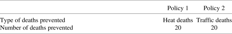
Which of the two policies would you vote for?
-
○ 20 fewer heat deaths
-
○ 20 fewer traffic deaths
-
○ Both equally good
The first question in the policy comparison set introduced respondents to the survey format and served as an attention check. Subjects were randomly assigned to consider either two policies that would reduce extreme heat risks or two policies that would reduce cancer or traffic risks, consistent with subjects’ group assignment. The risk presented in the introductory question was randomized to avoid any bias arising from subjects inferring that the study’s primary interest was heat risks. Under the first policy, fatalities would decrease by 20 while the second policy would decrease fatalities by 50. Policy 2 strictly dominated Policy 1, which should lead all rational subjects that understand the question to choose Policy 2. If subjects voted for Policy 1 or stated that both policies were equally good, they were asked to reconsider, for example, as follows: “You chose Policy 1. Under Policy 1, 20 deaths from extreme heat are prevented. Under Policy 2, 50 deaths from extreme heat are prevented.” The survey then presented another table analogous to the one above, and asked, for example, “Are you sure that you prefer Policy 1?” Respondents that answered correctly initially or upon reconsideration are retained in the analyses, while respondents that confirmed their initially dominated answer are excluded.Footnote 3
The next five policy questions directly asked subjects to choose between policies that would decrease heat fatalities and either cancer or traffic fatalities by 20, 30, or 50 deaths, as in the example question above. Respondents considered a series of five different tradeoff combinations: (20, 20), (20, 30), (30, 20), (50, 20), and (20, 50). The fatality values permit the questionnaire to identify relative mortality risk valuations ranging from 0.4 to 2.5, covering a wide range of premia that include the tradeoff rates in Alberini and Šcasný (Reference Alberini and Šcasný2024) and Chilton et al. (Reference Chilton, Duxbury, Mussio, Nielsen and Sharma2024). Further, the relative ratios of the risks are similar to those used in prior risk-risk studies and are analogous to the risk magnitudes used in dichotomous choice studies to measure subjects’ willingness to pay for heat-related mortality risks (Alberini, Reference Alberini2005; Chilton et al., Reference Chilton, Duxbury, Mussio, Nielsen and Sharma2024). By comparing two different types of fatal risks, the survey captures respondent preferences associated with both the mortality and morbidity components of the different causes of death.
The five isolated heat tradeoff questions provide the data for our core findings regarding the relative value of heat fatalities and also provide a transitivity check for respondents. For example, if a rational subject voted to reduce heat fatalities when the tradeoff was 20 heat fatalities and 20 cancer fatalities, the same subject should prefer to reduce heat fatalities when the tradeoff is 30 or 50 heat fatalities and 20 cancer fatalities. We exclude respondents who violate transitivity from the following main analysis.Footnote 4
The next six questions asked subjects to choose between policies that would decrease fatalities, with the added dimension that each question randomly assigned the heat or secondary risk to reduce senior citizen fatalities, while the comparison risk reduced fatalities among the general population. The survey’s stated justification for the policy to exclusively benefit senior citizens was that one of the two grants must be used to treat patients on Medicare. The first of the six questions in this set asked respondents to compare two policies that both reduced fatalities from heat, but one policy targeted senior citizens, while the other targeted members of the general population. The remaining five questions resembled the prior policy questions, in that one policy targeted heat risks, while the other targeted cancer or traffic risks. The introductory text to the second block of policy questions is as follows:
The following questions also present us with the option to choose between two different government policies that reduce fatalities from various causes.
As before, the questions will present us with two policies that provide grants to hospitals which have an above-average number of patients suffering from extreme heat or cancer. A grant to hospitals treating an above-average number of patients suffering from a particular condition will still reduce the fatality risk to those patients. And, as before, both policies cost the same amount.
In addition, the grants in the following policies may be provided to hospitals on the condition that they exclusively use them to improve treatments for patients on Medicare. Medicare patients are generally senior citizens who are 65 and older. As a result, those policies will decrease the fatality risk to senior citizens of extreme heat or cancer.
The text of the question that followed the preceding vignette is as follows:
Suppose that the outcome under each of the two policies is as follows.
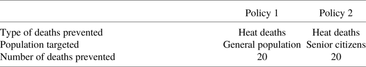
Which of the two policies would you vote for?
-
○ 20 fewer heat deaths
-
○ 20 fewer traffic deaths
-
○ Both equally good
Finally, the survey concluded by asking subjects a series of demographic and behavioral questions. The demographic questions included questions about respondents’ age, gender, race, education, income, marital status, whether they have minor children, and the zip code in which they live. Subjects’ zip codes provided the basis for determining the historical average high temperatures and the high temperatures during the week we fielded out survey in the area where subjects live. Data on daily high temperatures are from the Daily Global Historical Climatology Network. We match subjects to the nearest weather station in the Network to determine the high temperatures subjects faced. The behavioral questions elicited information that could be relevant to how respondents think about heat risks, including who they voted for in 2020, whether they have air conditioning in their home, whether they received a COVID-19 vaccine, whether they are smokers, whether they always or almost always wear a seatbelt, and whether they regularly engage in outdoor work or recreation. The survey concluded by asking subjects whether they found the questions in the survey clear or confusing.Footnote 5
2.2. Sample
After a series of pretests, the Prolific platform administered the survey to its panel of respondents. Prolific actively maintains a pool of more than 85,000 active U.S.-based survey respondents (as of July 2024), where membership in the panel excludes participants with low-quality responses. Prior research has found that Prolific respondents perform better than respondents from other platforms and panels, such as Amazon’s Mechanical Turk or Dynata (Peer et al., Reference Peer, Rothschild, Gordon, Evernden and Damer2022). The full sample consisted of 1,170 respondents. The sample that we used decreased to 1,048 respondents after excluding the 122 respondents who failed the attention and transitivity checks discussed in Section 2.2, or who chose the same answer in response to all policy choice questions (e.g., choosing “both equally good” for all 11 questions after the attention check).Footnote 6
We fielded the survey to two different samples: a general sample representative of the United States population along gender, race and ethnicity, and age dimensions, and a smaller sample of respondents of senior citizens whose age was 65 or greater. As discussed previously, heat presents a more serious risk for older adults, as measured in U.S. government heat death statistics. Heat may therefore be a more salient risk for senior respondents. Oversampling senior citizens permits us to explore how salience and personal exposure to the risk influences subjects’ preferences. To be sure, other risks, including mortality risks from extreme cold, are likely also more salient to seniors than other populations.Footnote 7 However, it seems unlikely that one category of salient risks for seniors should crowd out other salient risks, particularly given that senior citizens are a population who experience larger fatality risks from many causes. As a result, we expect that if heat is a salient risk to any particular group, it may be to seniors.
The sample includes a diverse set of respondents that parallel the U.S. population, conditional on the intentional oversampling of senior citizens. Female respondents, respondents who have a bachelor’s degree or higher, and respondents that voted for Joe Biden or voted at all in 2020 are somewhat overrepresented relative to the U.S. population. As described in the next subsection, most individual characteristics do not enter the model explicitly because of the panel structure of the data and the structure of the conditional logit model. The full set of summary statistics is provided in Table A1 in the Online Appendix.
Respondents took the questionnaire during the week of June 18, 2024. During that week, abnormally high temperatures affected much of the United States. Buffalo, New York, for example, had daytime high temperatures that were higher than Austin, Texas on June 19, 2024. The sharp increase in temperatures that week serves as an exogenous shock that enables identification of how subjects’ preferences over extreme heat risks vary with unexpected increases in the outdoor temperature. It also had the benefit of increasing the salience of the risks the survey explored, increasing the likelihood that respondents provided authentic preferences. To be sure, fielding the survey during a heat wave could have inflated subjects’ preferences to reduce heat risks rather than other mortality risks. If subjects’ valuations of heat risks are at their highest point during a heat wave, this situation should provide a favorable context for whether U.S. respondents place a valuation premium on mortality risk reductions from heat, as compared to mortality risks from transportation or cancer.
2.3. Random utility model
The stated preference survey design provides data to estimate a random utility model. Other papers in the literature analyzing risk-risk tradeoffs frequently rely on similar models (e.g., Viscusi, Reference Viscusi2009; Dalafave & Viscusi, Reference Dalafave and Viscusi2021). The survey presents respondents with a series of discrete policy choices involving the number of heat deaths prevented and either the number of cancer or traffic deaths prevented. The stated preferences from these choices can be used in a random utility framework to analyze subjects’ utility tradeoffs between the relevant fatality risks.
Consider a representative individual with preferences over mortality risks from different causes.Footnote 8 For any policy $ i $
, individual preferences correspond to a utility function that varies with mortality risk reductions and individual characteristics, and includes a random component. Let
$ i $
, individual preferences correspond to a utility function that varies with mortality risk reductions and individual characteristics, and includes a random component. Let $ {h}_i $
represent the reduction in heat deaths,
$ {h}_i $
represent the reduction in heat deaths, $ {c}_i $
represent the reduction in cancer deaths, and
$ {c}_i $
represent the reduction in cancer deaths, and $ {t}_i $
represent the reduction in traffic deaths from policy
$ {t}_i $
represent the reduction in traffic deaths from policy $ i $
. Let the vector
$ i $
. Let the vector $ {x}_n $
represent an individual’s demographic characteristics and let
$ {x}_n $
represent an individual’s demographic characteristics and let $ {\epsilon}_{ni} $
be the random component of utility for individual
$ {\epsilon}_{ni} $
be the random component of utility for individual $ n $
from policy
$ n $
from policy $ i $
. Then an individual’s utility function for a given policy can be expressed as follows:
$ i $
. Then an individual’s utility function for a given policy can be expressed as follows:
 $$ {u}_{ni}=\alpha {h}_i+\beta {c}_i+\gamma {t}_i+\delta {x}_n+{\epsilon}_{ni}. $$
The absolute value of utility $ {u}_{ni} $
is not of primary interest, as utility levels are unique only up to a positive linear transformation, but the marginal rate of substitution between the different risk categories is. Totally differentiating
$ {u}_{ni} $
is not of primary interest, as utility levels are unique only up to a positive linear transformation, but the marginal rate of substitution between the different risk categories is. Totally differentiating $ {u}_{ni} $
along the policy dimensions yields:
$ {u}_{ni} $
along the policy dimensions yields:
 $$ 0=\alpha \mathrm{dh}+\beta \mathrm{dc}+\gamma \mathrm{dt}. $$
The marginal rate of substitution between heat fatalities and cancer fatalities is accordingly $ -\alpha /\beta $
, while the marginal rate of substitution between heat and traffic fatalities is
$ -\alpha /\beta $
, while the marginal rate of substitution between heat and traffic fatalities is $ -\alpha /\gamma $
. If, for example,
$ -\alpha /\gamma $
. If, for example, $ -\alpha /\beta =2 $
, respondents would be indifferent between a policy that reduced their heat fatality risk by 2/1,000 and cancer fatalities by 1/1,000. It follows that if respondents would be willing to pay $10,000 to decrease their cancer fatality risk by 1/1,000, they would be willing to pay $20,000 to decrease their heat fatality risk by 1/1,000, assuming that relevant income effects are sufficiently small. The marginal rate of substitution consequently provides the value of heat fatalities relative to cancer or traffic fatalities.
$ -\alpha /\beta =2 $
, respondents would be indifferent between a policy that reduced their heat fatality risk by 2/1,000 and cancer fatalities by 1/1,000. It follows that if respondents would be willing to pay $10,000 to decrease their cancer fatality risk by 1/1,000, they would be willing to pay $20,000 to decrease their heat fatality risk by 1/1,000, assuming that relevant income effects are sufficiently small. The marginal rate of substitution consequently provides the value of heat fatalities relative to cancer or traffic fatalities.
To recover the marginal rates of substitution of interest, we exploit the fact that individuals vote for the policy that yields greater utility when asked to choose between multiple policies. Symbolically, from equation 1, an individual chooses policy $ j $
over policy
$ j $
over policy $ i $
if:
$ i $
if:
 $$ {u}_{nj}>{u}_{ni}\iff \alpha \left({h}_j-{h}_i\right)+\beta \left({c}_j-{c}_i\right)+\gamma \left({t}_j-{t}_i\right)+{\epsilon}_{nj}-{\epsilon}_{ni}>0. $$
Because individual characteristics $ {x}_n $
are common to all policy options, they are not included in the basic model.Footnote 9 In the survey, policies affect reductions from only a single fatality type, and subjects compare heat and only one of the two alternatives. For ease of exposition, assume that policy
$ {x}_n $
are common to all policy options, they are not included in the basic model.Footnote 9 In the survey, policies affect reductions from only a single fatality type, and subjects compare heat and only one of the two alternatives. For ease of exposition, assume that policy $ i $
affects heat, policy
$ i $
affects heat, policy $ j $
affects cancer, and policy
$ j $
affects cancer, and policy $ k $
affects traffic. Then Equation 2 simplifies to the following two possible comparisons:
$ k $
affects traffic. Then Equation 2 simplifies to the following two possible comparisons:
 $$ {u}_{nj}>{u}_{ni}\iff -\alpha {h}_i+\beta {c}_j+{\epsilon}_{nj}-{\epsilon}_{ni}>0, $$
and
 $$ {u}_{nk}>{u}_{ni}\iff -\alpha {h}_i+\gamma {t}_k+{\epsilon}_{nk}-{\epsilon}_{ni}>0. $$
The probability $ {p}_{nji} $
or
$ {p}_{nji} $
or $ {p}_{nki} $
that an individual prefers policy
$ {p}_{nki} $
that an individual prefers policy $ i $
to policy
$ i $
to policy $ j $
or
$ j $
or $ k $
for any policy comparison is correspondingly:
$ k $
for any policy comparison is correspondingly:
 $$ {p}_{nji}=\mathrm{P}\mathrm{r}\mathrm{o}\mathrm{b}(-\alpha {h}_i+\beta {c}_j+{\epsilon}_{nj}-{\epsilon}_{ni}>0), $$
and
 $$ {p}_{nk i}=\mathrm{Prob}\left(-\alpha {h}_i+\gamma {t}_k+{\epsilon}_{nk}-{\epsilon}_{ni}>0\right). $$
The regression analysis presents estimates of equations 4a and 4b using a conditional logit model. The model simultaneously estimates equations 4a, 4b, and an equation corresponding to indifference between the two policy options.Footnote 10 Simultaneously estimating the two equations of interest and the equation corresponding to indifference between the two options maximizes the precision of our estimates. The results for the “both equally good” choice regressions are reported in the Online Appendix, but are not a focus in the main results reported in the analysis. The observations in the regression are each policy choice that subjects considered (the policy reducing heat deaths, the policy reducing other deaths, and expressing that both policies were equally good). The panel model accounts for using multiple observations per individual by clustering the estimated standard errors by individual respondent.
The output of the conditional logit model enables identification of how the subjects value heat mortality risks relative to cancer and traffic risks. The coefficients in the model provide the marginal utility of choosing one policy alternative relative to the marginal utility of choosing another. The marginal utilities are of directional interest as they demonstrate whether respondents are responding rationally to the survey instrument, but their magnitudes are not meaningful in isolation. The ratio of the coefficients within an equation, however, provide marginal rates of substitution between different sources of utility (McFadden & Train, Reference McFadden and Train2000), such as the mortality risks in the model. The ratios of the coefficients for the magnitude of fatalities averted accordingly provide the relative valuations of heat fatalities to cancer and traffic fatalities.
Beyond the basic model in equations 1–4, we make several additional refinements to the analysis. At various points, we relax the implicit assumption that the parameters $ \alpha $
,
$ \alpha $
, $ \beta $
, and
$ \beta $
, and $ \gamma $
are comparable across groups of respondents and separately estimate equations 4a and 4b for members of the samples who are older or younger than 65, who live in higher temperature areas, or who experienced higher heat shocks during the heat wave. We also investigate whether individual characteristics such as respondents’ beliefs about their own risk of suffering from heat affect their relative valuation of heat fatalities by including interactive effects in the regression model. Such refinements add additional terms to the equations above but do not alter the fundamental structure of the model. And in the Online Appendix, we report results that relax the assumption that utility is linear in risk levels.Footnote 11
$ \gamma $
are comparable across groups of respondents and separately estimate equations 4a and 4b for members of the samples who are older or younger than 65, who live in higher temperature areas, or who experienced higher heat shocks during the heat wave. We also investigate whether individual characteristics such as respondents’ beliefs about their own risk of suffering from heat affect their relative valuation of heat fatalities by including interactive effects in the regression model. Such refinements add additional terms to the equations above but do not alter the fundamental structure of the model. And in the Online Appendix, we report results that relax the assumption that utility is linear in risk levels.Footnote 11
In sum, the experimental questionnaire is calibrated to produce results that are likely to demonstrate subjects’ authentic preferences regarding heat-related mortality risks.Footnote 12 The instrument includes several rationality checks, which respondents overwhelmingly passed. The tabulations of subjects’ responses demonstrate that they pass scope tests, which the analyses in Part III further illustrate.Footnote 13 And most importantly, the structure and timing of the survey experimentally randomize our subjects into groups to test our major hypotheses: whether subjects have a heat valuation premium, whether exogenous heat shocks affect heat mortality valuation, and whether subjects differentially value risks to senior citizens.
3. Results
3.1. Policy choices and the relative valuation of heat risks
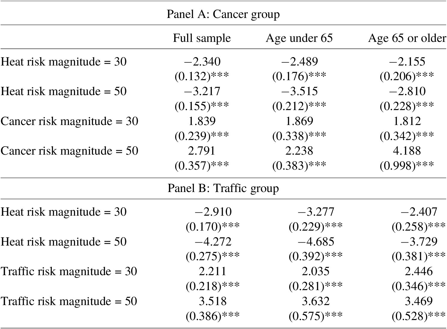
The analysis begins with the basic results demonstrating that respondents provide no evidence of a heat valuation premium. Table 1 presents three different conditional logit regressions for both the heat-cancer and heat-traffic tradeoffs for three different samples: the full sample, the age under 65 years subsample, and the age 65 years or older subsample. Each coefficient represents the estimated change in the log-odds that a respondent votes for a policy reducing the identified secondary risk (i.e., cancer or traffic) relative to the log-odds of voting for a policy that reduces heat-related fatalities, in response to a one-unit increase in the magnitude of lives saved from heat or the secondary risk in the policy trade-off question. The bottom section of Table 1 reports the implied value of heat fatalities relative to cancer and traffic fatalities, calculated as the negative of the ratio of the two estimated coefficients, along with the associated 95% confidence intervals.Footnote 14
Table 1. Policy choice regressions
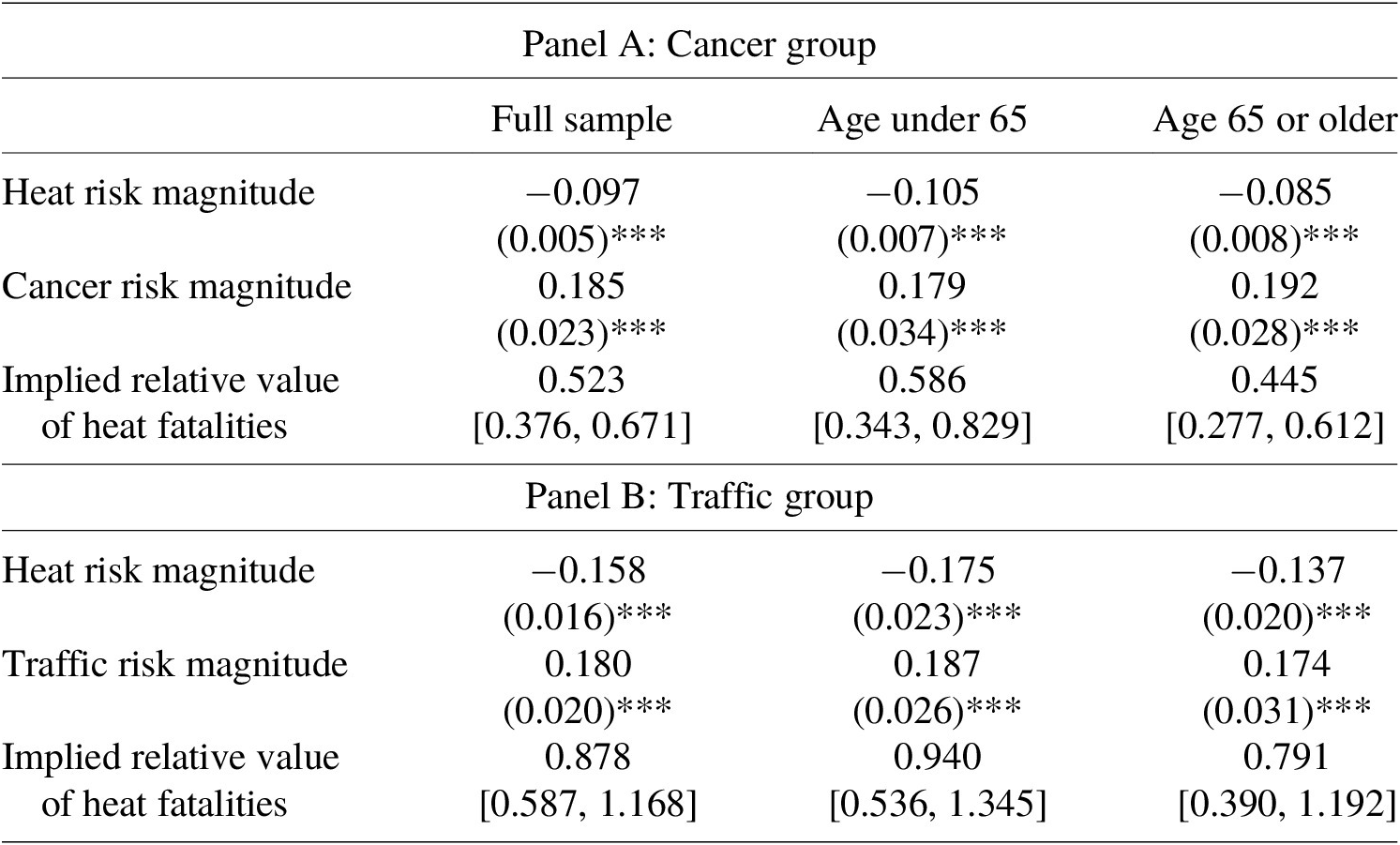
Note: Table 1 reports the estimated coefficients in a conditional logit choice model modeling the likelihood that respondents vote to reduce cancer or traffic deaths with reducing heat deaths as the base option. Standard errors are robust and clustered on respondent. 95% confidence intervals for implied relative heat valuations are provided in brackets and calculated using the delta method. N = 15,720 for the full sample, 9,450 for the age under 65 subsample, and 6,270 for the 65 or over subsample. ***p < 0.01, **p < 0.05, *p < 0.10.
The core finding is that the evidence does not establish any valuation premium for heat mortality risks over cancer or traffic fatality risks. There is a clearcut premium for cancer risks relative to heat risks, and there is no statistically significant difference in the heat and traffic fatality valuations. As expected, the estimated coefficient on the change on heat risk is statistically significant and negative, while the coefficients on cancer and traffic risks are statistically significant and positive, consistent with responses passing a scope test. The ratio of the coefficients on heat and cancer in the full sample cancer equation was 0.52, implying that subjects were indifferent between preventing approximately two cancer fatalities and one heat fatality. The relative valuation of 0.52 is significantly different from 1.0 ( $ p<0.001 $
). The large premium on cancer fatalities relative to heat (and implicitly, traffic) is consistent with the literature finding that subjects place a premium on cancer fatalities relative to other risks. In contrast, the point estimate for the ratio for heat and traffic mortality was 0.88, but it is statistically indistinguishable from 1.0 (
$ p<0.001 $
). The large premium on cancer fatalities relative to heat (and implicitly, traffic) is consistent with the literature finding that subjects place a premium on cancer fatalities relative to other risks. In contrast, the point estimate for the ratio for heat and traffic mortality was 0.88, but it is statistically indistinguishable from 1.0 ( $ p=0.409\Big) $
. Subjects did not prefer to prevent heat fatalities over traffic fatalities, which are a representative benchmark for traumatic mortality risks in the risk-risk valuation literature (e.g., Viscusi et al., Reference Viscusi, Magat and Huber1991).Footnote 15 In short, we find no evidence of a premium for heat fatalities over other mortality risks. However, the confidence intervals on the implied relative heat valuations are sufficiently large to be consistent with a heat premium for traffic as large as approximately 15%, or a penalty as large as approximately 40%. The remaining columns in Table 1 indicate that there is little difference between how our younger and older subsamples value heat-related mortality risks relative to cancer or traffic.
$ p=0.409\Big) $
. Subjects did not prefer to prevent heat fatalities over traffic fatalities, which are a representative benchmark for traumatic mortality risks in the risk-risk valuation literature (e.g., Viscusi et al., Reference Viscusi, Magat and Huber1991).Footnote 15 In short, we find no evidence of a premium for heat fatalities over other mortality risks. However, the confidence intervals on the implied relative heat valuations are sufficiently large to be consistent with a heat premium for traffic as large as approximately 15%, or a penalty as large as approximately 40%. The remaining columns in Table 1 indicate that there is little difference between how our younger and older subsamples value heat-related mortality risks relative to cancer or traffic.
Differences in the studied population and environment likely account for the differences between the results and those of Chilton et al. (Reference Chilton, Duxbury, Mussio, Nielsen and Sharma2024) and Alberini and Šcasný (Reference Alberini and Šcasný2024). For example, with regard to Chilton et al. (Reference Chilton, Duxbury, Mussio, Nielsen and Sharma2024) which focused on India, prior literature has found sizeable macroeconomic and mortality effects of heat in middle- and lower-income economies, including India (e.g., Robinson et al., Reference Robinson, Hammitt, Cecchini, Chalkidou, Claxton, Cropper, Eozenou, de Ferranti, Deolalikar, Guanais, Jamison, Kwon, Lauer, O’Keeffe, Walker, Whittington, Wilkinson, Wilson and Wong2019; Liu et al., Reference Liu, Shamdasani and Taraz2023). Such differences could induce different valuations, just as cultural differences and greater concern with the impact of global warming could explain differences between a U.S. sample and the European sample in Alberini and Šcasný (Reference Alberini and Šcasný2024). It is also possible that differences in the framing of our questionnaire, such as by creating mortality risk reductions through hospital grants, could explain some of the discrepancy. For example, some have suggested that most heat fatalities occur before individuals reach the hospital, which may have affected how sophisticated respondents reacted to the questionnaire (e.g., Sun et al., Reference Sun, Weinberger, Nori-Sarma, Spangler, Sun, Dominici and Wellenius2021).
3.2. Temperature and heat evaluations
It is also feasible to experimentally identify how subjects’ responses vary with the temperature they experience and how those temperatures relate to their own perceived risks of heat fatalities. The temperatures that respondents experience may directly influence their valuation of heat risks in a variety of ways. First, being exposed to heat may lead subjects to assess the mortality risk change that is pertinent to them differently than instructed in the questionnaire. Temperature may even negatively affect subjects’ cognitive performance (Zivin et al., Reference Zivin, Song, Tang and Zhang2020). Second, heat may also affect respondents’ perception of the morbidity risks from heat, which in turn may lead them to assess their personal risks from heat as being different than the risk levels stated in the survey.
To analyze how stated preferences for heat risks vary with actual temperatures, historical average daily high temperatures are used to assess the relationship between expected historical temperatures and preferences over mortality risks. The extent of deviation from those expected historical temperatures serves as the measure of the heat shock on individual preferences. We measure historical temperatures as the average daily high between June 17 and June 24 in 2021, 2022, and 2023 at the weather station nearest to a respondent’s zip code. The size of the shock from the heat wave is given by difference between the average daily high temperature between June 17 and 24 in 2024, the week subjects took the survey, and the historical temperature.
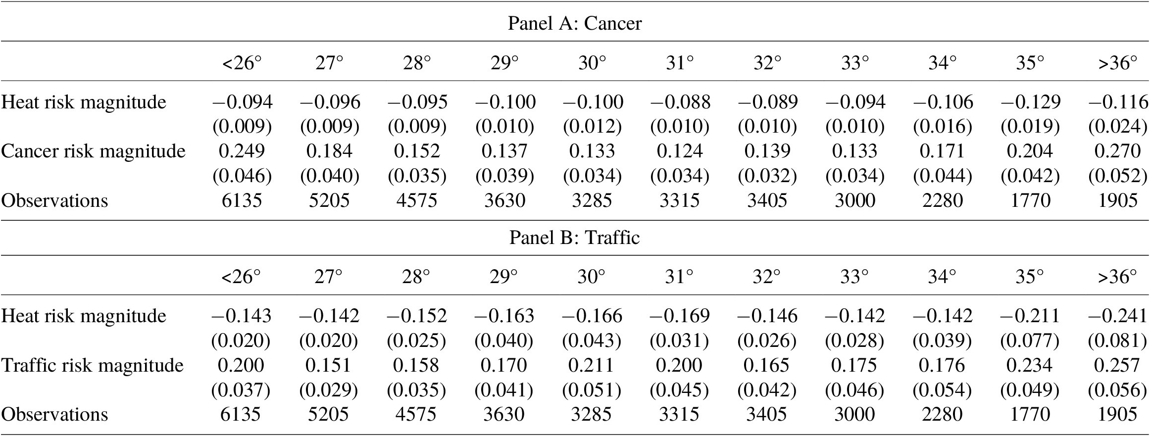
Figures 1 and 2 illustrate the estimates that examine the relationship between heat and heat risk valuations, which are based on conditional logit regressions reported in full in Table A5 and A6 of the Online Appendix. In both figures, each point on the central line is the value of heat relative to either cancer or traffic for respondents whose zip code has an average historical daily high temperature within 1.5 °C of the benchmark value.Footnote 16 In other words, the figure shows a moving average of the relationship between historical temperatures and heat valuations. The top and bottom lines represent the upper and lower bounds of the 95% confidence interval corresponding to each estimate. Figure 2, in turn, presents the relative heat valuations when respondents are grouped according to the size of the heat shock they experienced during the June 2024 heat wave. The horizontal axis identifies the degrees Celsius by which the average daytime high during the heatwave varied from the historical average high in that area. Analogously to Figure 1, each point on the line corresponds to the results from a conditional logit model for respondents whose zip code experienced a deviation from their usual daytime highs within 1.5 °C of the listed value.
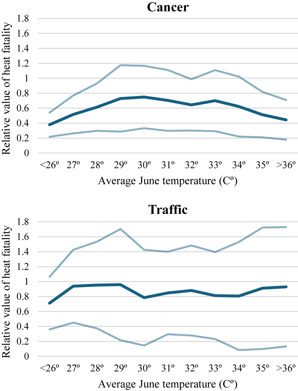
Figure 1. Historical temperatures and relative valuation of heat fatalities.
Note: Each point on the central line is the ratio of coefficients from the conditional logit model, restricted to respondents living in zip codes with average daily high temperatures within 1.5 °C of the relevant temperature. Average daily high temperatures are measured over June 17–24 in 2021–2023. The other lines present 95% confidence intervals.
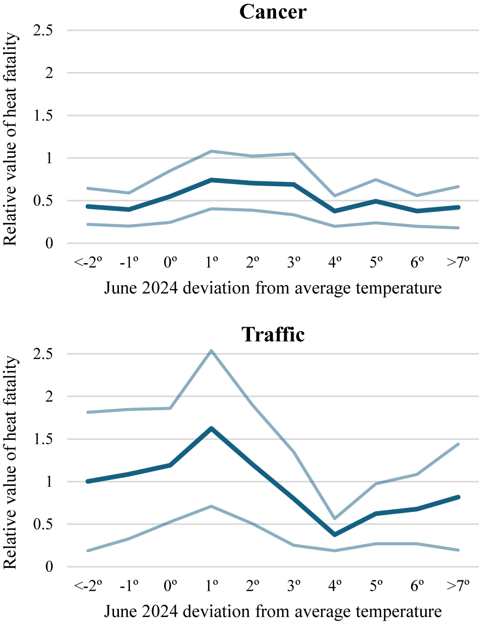
Figure 2. Heat wave temperatures and relative valuation of heat fatalities.
Note: Each point on the central line is the ratio of coefficients from the conditional logit model, restricted to respondents living in zip codes with average daily high temperatures within 1.5 °C of the relevant temperature. Average daily high temperatures are measured over June 17–24 in 2024. The other lines present 95% confidence intervals.
Figure 1 demonstrates that temperature expectations based on historical averages for that period have a relatively weak relationship with subjects’ preferences with respect to heat risks and other mortality risks. In Figure 1, the valuation of heat relative to cancer and traffic does not increase or decrease much as expected daytime high temperatures increase, suggesting that individual preferences over mortality risks from heat do not vary with expected individual heat exposure. The result is encouraging – if subjects treated the risks in the questionnaire as reflecting their personal risk level, historical exposure to greater heat should not be associated with different valuations. No temperatures within the observed range yield a relative valuation of mortality risks from heat that is statistically greater than 1.0.
Figure 2 shows that even exogenous shocks to high temperatures do not have a substantial effect on preferences with respect to heat risks. Respondents’ valuation of heat risks relative to cancer were between 0.3 and 0.5 for respondents living in areas that did not get warmer during the heat wave. Respondents whose temperatures increased by approximately 1 °C to 3 °C demonstrated an increased relative valuation of 0.6. But the value of heat relative to cancer decreased back to between 0.3 and 0.5 for respondents whose temperatures increased by approximately more than 4° during the heat wave. Subjects’ valuation of heat mortality risks relative to traffic risks follow a similar pattern. U.S. respondents may exhibit weakly inverted U-shaped preferences with respect to temperature shocks.
Some other articles in the risk-risk literature have found that subjects’ perceived mortality risks affect their relative valuations (e.g., Dalafave & Viscusi, Reference Dalafave and Viscusi2021; Chilton et al., Reference Chilton, Duxbury, Mussio, Nielsen and Sharma2024). Here we link these subjective risk perceptions of heat risks to objective measures of historical temperatures. A plausible mechanism by which experienced temperatures affect relative valuations is that the temperatures influence individual risk beliefs regarding heat risks, which in turn alter their assessment of the personal risk reduction that they will experience from the policy options presented in the survey. To investigate this issue, Table 2 estimates a logit model in which the dependent variable is a binary variable equal to 1 if a respondent stated they have an above average heat risk. The independent variables of interest are the measures of temperatures studied in Figures 1 and 2: the historical average daily high temperature in a respondent’s zip code from June 17–24 in 2021, 2022, and 2023, and the number of degrees Celsius that the average daily high between June 17 and 24 in 2024 exceeded the historical average. The first column of Table 2 presents a basic version of the logit model, while the model in the second column also includes controls for individual demographic variables.
Table 2. Perceived above average heat risk and temperatures
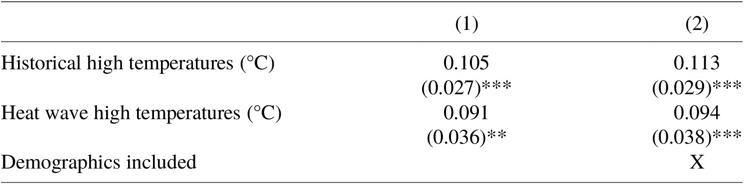
Note: N=1,048. Dependent variable in the logit regressions is a binary variable equal to 1 if respondent stated that they have an above average risk of dying from heat. Robust standard errors are in parentheses. ***p < 0.01
The results in Table 2 are consistent with passing a behavioral scope test: subjects’ perceived heat-related mortality risk is increasing in the historical temperatures where they live as well as the temperature shock they experienced during the heat wave. The two coefficients are similar in magnitude, with a 1 °C change in either variable implying an approximately 10% increase in the probability of reporting an above average risk of heat mortality. As expected, higher temperatures lead subjects to believe they have a higher risk of heat-related mortality.
Risk beliefs for heat, cancer, and traffic may possibly affect respondents’ tradeoffs for these risks. Among our subjects, 16.5% of respondents report an above average risk of dying of heat, 14.7% report an above average risk of dying due to cancer, and only 3.9% report an above average risk of dying from a traffic fatality. The 3.9% traffic result is consistent with the classic result from the behavioral economics literature that individuals report an irrationally optimistic view of their own driving abilities (e.g., Taylor, Reference Taylor1990), which in turn may affect their perceived risk of motor-vehicle deaths.
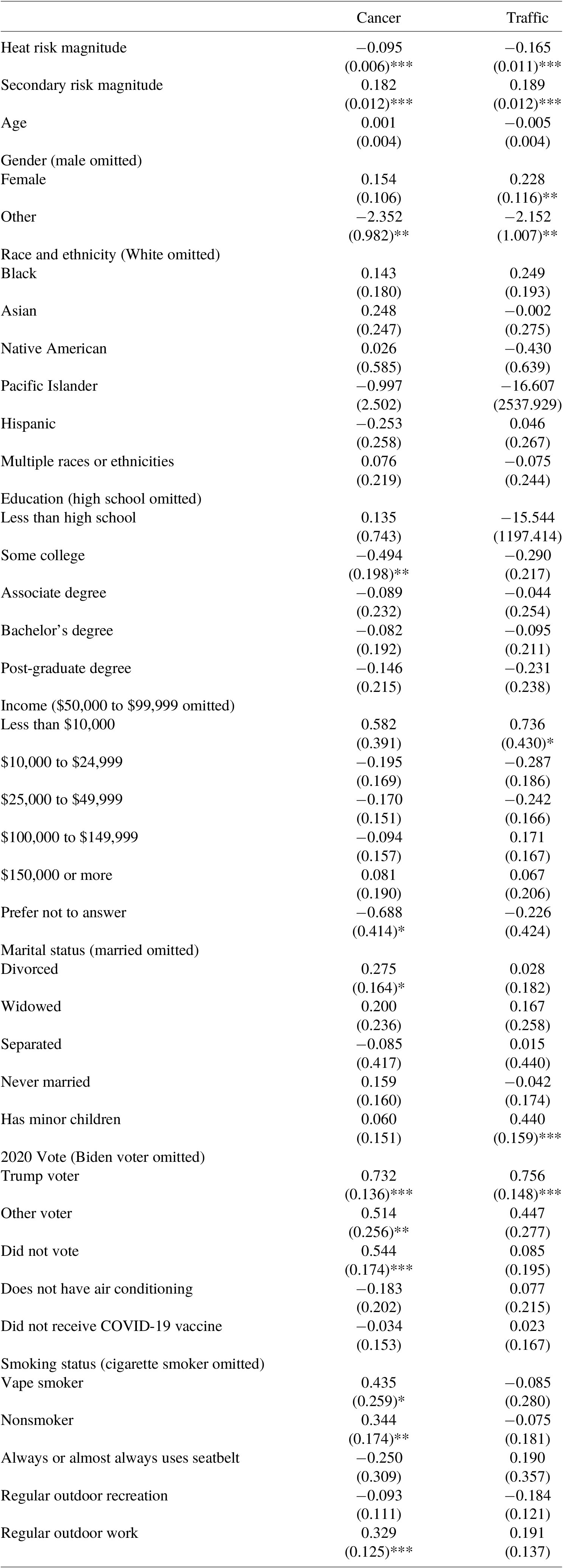
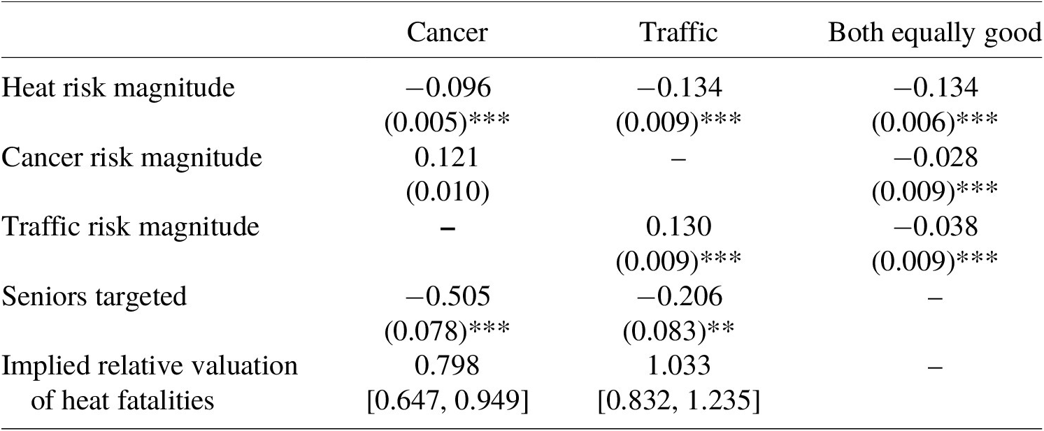
Table 3 presents the conditional logit model estimates including interaction terms for subjects’ own perceived fatality risk beliefs. The two interaction terms corresponding to high heat and secondary fatality risk are binary variables equal to one if a subject reported that they have an above-average risk of dying due to heat or the secondary risk the subject considered, and zero otherwise – the same as the dependent variable from Table 2.Footnote 17 A high-risk individual’s estimated marginal utility from a given policy is accordingly the sum of the coefficient on the risk magnitude variable and the interaction term between risk magnitude and high risk.
Table 3. Policy preferences and perceived own fatality risk
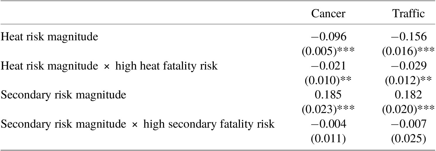
Note: N = 15,620. Table 3 reports the estimated coefficients in a conditional logit choice model modeling the likelihood that respondents vote to reduce cancer or traffic deaths with reducing heat deaths as the base option. Standard errors are robust and clustered on respondent. 95% confidence intervals for implied relative heat valuations are provided in brackets and calculated using the delta method. ***p < 0.01, **p < 0.05, *p < 0.10.
The results in Table 3 imply that subjects with higher perceived heat fatality risks exhibited a greater preference for reducing heat fatalities.Footnote 18 The coefficient on heat risk magnitude is statistically significant, negative, and adds approximately 20% to the marginal utility of decreasing heat fatalities. The significant interactive relationship between an individual’s perceived risk and their relative valuation of heat risks is striking given the weak relationship between actual experienced heat and relative valuations shown in Figure 1. The results in Table 3 indicate that the respondents did not entirely differentiate between the risks to the public in the questionnaire and the risks to themselves, with high-heat risk individuals expressing a greater preference to prevent fatalities to others. Individuals with a high perceived own risk of heat mortality are indifferent between reducing 0.63 cancer fatalities and 1 heat fatality, compared to 0.51 for individuals who do not perceive a high risk for themselves. Both the elevated high-risk and general risk estimate remain significantly different from 1.0, however ( $ p<0.001\Big) $
. Even subjects who believe they have higher than average heat-related mortality risks place a premium on cancer risks above heat risks. Similarly, the point estimate for the relative value of heat fatalities for the traffic group was 1.01 among individuals with a perceived high risk of heat fatalities, and 0.86 among the remainder of the sample. Both values are not significantly different from 1.0 (
$ p<0.001\Big) $
. Even subjects who believe they have higher than average heat-related mortality risks place a premium on cancer risks above heat risks. Similarly, the point estimate for the relative value of heat fatalities for the traffic group was 1.01 among individuals with a perceived high risk of heat fatalities, and 0.86 among the remainder of the sample. Both values are not significantly different from 1.0 ( $ p=0.940 $
and
$ p=0.940 $
and $ p=0.315\Big) $
. In contrast to the higher relative value for heat due to higher self-perceived risk, the coefficients on cancer risk and traffic risk interacted with subjects’ self-perceived risk were never statistically significant.
$ p=0.315\Big) $
. In contrast to the higher relative value for heat due to higher self-perceived risk, the coefficients on cancer risk and traffic risk interacted with subjects’ self-perceived risk were never statistically significant.
3.3. Senior citizens and heat risks
This section analyzes the third question of primary interest: whether subjects differentially value risks to senior citizens and whether seniors have different valuations involving risks to themselves and risks to the general population. As discussed in Section 3.1, the initial results indicate that senior citizens and younger respondents have similar relative valuations of heat fatalities even though heat risks primarily affect senior citizens. Respondents did not value senior citizen fatalities less than fatality risks among the general population. The evidence reported below indicates that this finding is robust, and that there is no valuation penalty for senior citizens.
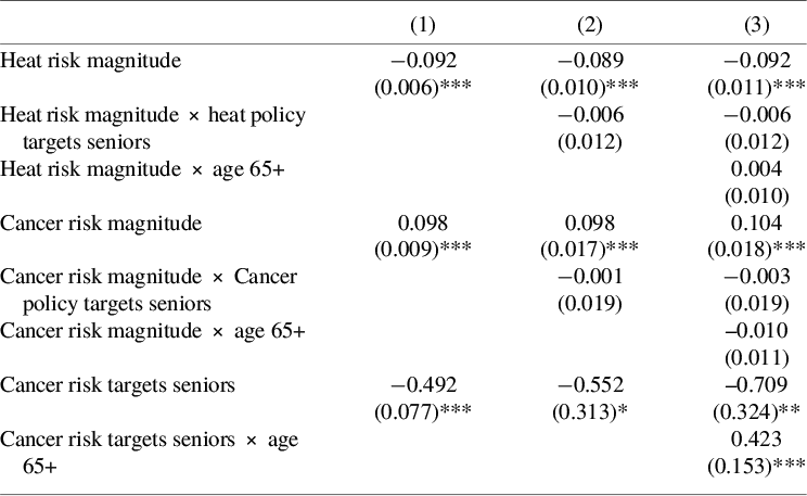
Tables 4A and 4B present the results of estimating the conditional logit model using data from the final block of policy questions in the survey which randomly varied whether the beneficiary of policies were senior citizens or the general population. Tables 4A and 4B correspond to responses to different questions from the same respondents as in the results for Tables 2 and 3. The six columns in Tables 4A and 4B present regression coefficients for six different equations from three regressions, with each of the three regressions adding more interactions with the risk magnitude variables to the estimating equation. Table 4A corresponds to policy preferences over cancer risks, while Table 4B corresponds to policy preferences over traffic risks. In both tables, the first columns estimate the basic model, adding only a term that shifts the intercept if the secondary risk targeted senior citizens. The second columns add interaction terms to each risk magnitude variable that permit the estimated response to risk magnitudes to vary if the risk targets seniors. The final columns interact each of the variables with a binary variable equal to one if the respondent’s age is 65 or greater.
Table 4A. Cancer policy preferences and targeted populations
Note: N = 15,720. Estimates represent the coefficient in a panel data conditional logit choice model estimating the probability that the respondent chose the policy reducing cancer or traffic deaths relative to the probability the respondent chose the policy reducing heat deaths. Standard errors are robust and clustered on respondent. ***p < 0.01, **p < 0.05, *p < 0.10.
Table 4B. Traffic policy preferences and targeted populations
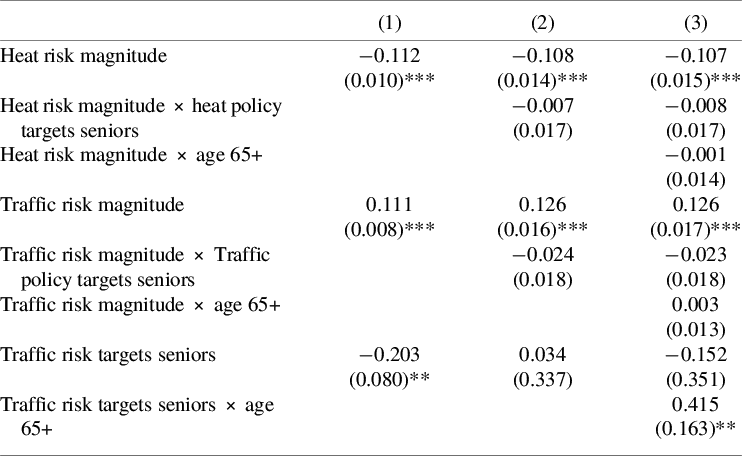
Note: N = 15,720. Estimates represent the coefficient in a panel data conditional logit choice model estimating the probability that the respondent chose the policy reducing cancer or traffic deaths relative to the probability the respondent chose the policy reducing heat deaths. Standard errors are robust and clustered on respondent. ***p < 0.01, **p < 0.05, *p < 0.10.
Tables 4A and 4B indicate that there is not a valuation penalty when the target beneficiary group is seniors rather than the general population. All the interactions between the binary senior targeting variable and the magnitude of the relevant risks are not statistically significant. There is no evidence that the subjects assigned a penalty or a premium valuation to these mortality risks to senior citizens. Nor did senior citizens’ valuation of any of the mortality risks differ significantly from that of other respondents, consistent with the earlier results in Table 1. The magnitudes of the heat risk and other coefficients are substantially closer to being equal than they were in Table 1, suggesting that subjects were less sensitive to mortality risk changes when also trading off beneficiary populations.Footnote 19 The results universally provide support that a heat risk penalty does not exist and that there is no senior penalty in these valuations for seniors based either on the population group being protected or the population group expressing the risk-risk preferences. It is possible that the frame of the questions – particularly that subjects were not told they were potential beneficiaries of any of the policies – may have contributed to the finding that senior citizens did not differentially value risks to senior citizens (Dolan et al., Reference Dolan, Olsen, Menzel and Richardson2003).
Although the tradeoff rates are not sensitive to whether the policy targets seniors, the intercept terms do vary. For cancer (and traffic in the basic model), respondents are less likely to choose the secondary non-heat-related risk when the protected group consists of seniors. The most likely explanation is that respondents simply disfavor voting for policies that only decrease senior fatalities without regard to the fatality risk tradeoffs because demographic targeting of policies is inequitable. Such a result is consistent with literature finding that individuals favor programs that benefit the general population rather than discrete groups (e.g., Card et al., Reference Card, Adshade, Hogg, Jollimore and Lachowsky2022). The statistically significant and positive coefficient on the interaction between the secondary risk targeting seniors and a respondent being older than 65 supports this explanation, as senior citizens are much less likely to have a blanket bias against a group to which they belong.
The results are consistent with respondents expressing preferences consistent with the equitable risks tradeoffs approach to the VSL for regulatory policy (Viscusi, Reference Viscusi2018; Kniesner & Viscusi, Reference Kniesner and Viscusi2024; Viscusi, Reference Viscusi2024). Based on that approach, regulatory agencies will use a population average VSL when evaluating policies affecting population-wide risks irrespective of the demographic composition of the beneficiary group. Using a subpopulation-specific VSL or distributional weights for different subpopulations is only appropriate if policies target subpopulations with differential preferences and the beneficiaries of the policy, in effect, pay for the policy benefit (Viscusi, Reference Viscusi2018; Kniesner & Viscusi, Reference Kniesner and Viscusi2023).
Indeed, there is further evidence of a substantial value of mortality risks to seniors based on the responses to the sixth policy choice question in the study, which asked subjects to choose between two Policies that reduce heat risks of equal magnitude, with one risk affecting the general population and one affecting senior citizens. Even when evaluating identical risks across the two groups, the majority of subjects viewed reducing mortality risks to seniors and the general population as being equivalent although subjects who indicated a preference were slightly more likely to select the policy benefitting the general population.Footnote 20 Overall, 253 respondents chose the policy benefitting the general population, 157 chose the policy benefiting senior citizens, and 638 respondents said both policies were equally good.
4. Conclusion
The experiment presents no evidence that U.S. subjects place a premium on valuations of mortality risks from heat. The valuation of heat-related mortality risk is not significantly different from that of traffic risks, which have a VSL that is not significantly different from that for other traumatic risks that most agencies use in establishing their VSL. Respondents consistently demonstrated across several analyses, including by exploiting exogenous shocks to subjects’ experienced temperatures, that they do not prefer reducing heat risks relative to other risks. Cancer risks do command a substantial mortality valuation premium, consistent with other evidence on the heterogeneity in the VSL. The results are consistent with the U.S. government’s current practice of not placing a premium on heat mortality risks when performing benefit-cost analyses of policies that may affect climate change or related risks, such as pricing the social cost of greenhouse gases (Carleton et al., Reference Carleton, Jina, Delgado, Greenstone, Houser, Hsiang, Hultgren, Kopp, McCusker, Nath, Rising, Rode, Seo, Viaene, Yuan and Zhang2022; EPA, 2023). Even without being accorded a valuation premium, the monetized value of heat-related mortality risks is substantial. The 2,262 U.S. heat-related deaths in 2023 represent more than $29.4 billion in social costs, using a U.S. value of statistical life of $13.0 million, and will likely continue to rapidly rise.Footnote 21
Whether the U.S. results generalize to other countries merits further exploration. Heat poses less of a mortality risk in countries in which air conditioning is prevalent and there is reliable electricity service. The findings by Chilton et al. (Reference Chilton, Duxbury, Mussio, Nielsen and Sharma2024) and Alberini and Šcasný (Reference Alberini and Šcasný2024) that heat-related deaths are valued more than traffic-related deaths in India and two European countries suggests that there may be a range of countries with relative valuations of heat deaths that are bounded between the absence of any premium in the U.S. and a substantial premium in India. Differences in methodology may also have contributed to the different results. Application of country results would be consistent with the recommendation by Fraas et al. (Reference Fraas, Graham, Krutilla, Lutter, Shogren, Thunström and Viscusi2023) that it is preferable to use the country’s valuations of greenhouse gas emissions.
The evidence presented here is consistent with benefit assessment practices that do not adjust the valuation of risks due to age differences in the beneficiaries of a policy. While subjects in this risk-risk study consistently demonstrated that they preferred policies that benefit the general population, the valuation of risk reductions for senior citizens and the general population was not significantly different. Both the full sample and the senior citizen subsample valued risks that targeted the general population and senior citizens similarly. Future research may reveal other dimensions on which regulatory benefit-cost analysis could adjust heat and other types of mortality risk valuations based on the heterogeneity of valuations.
Competing interests
The authors declare none.
Appendix
Table A1. Sample summary statistics
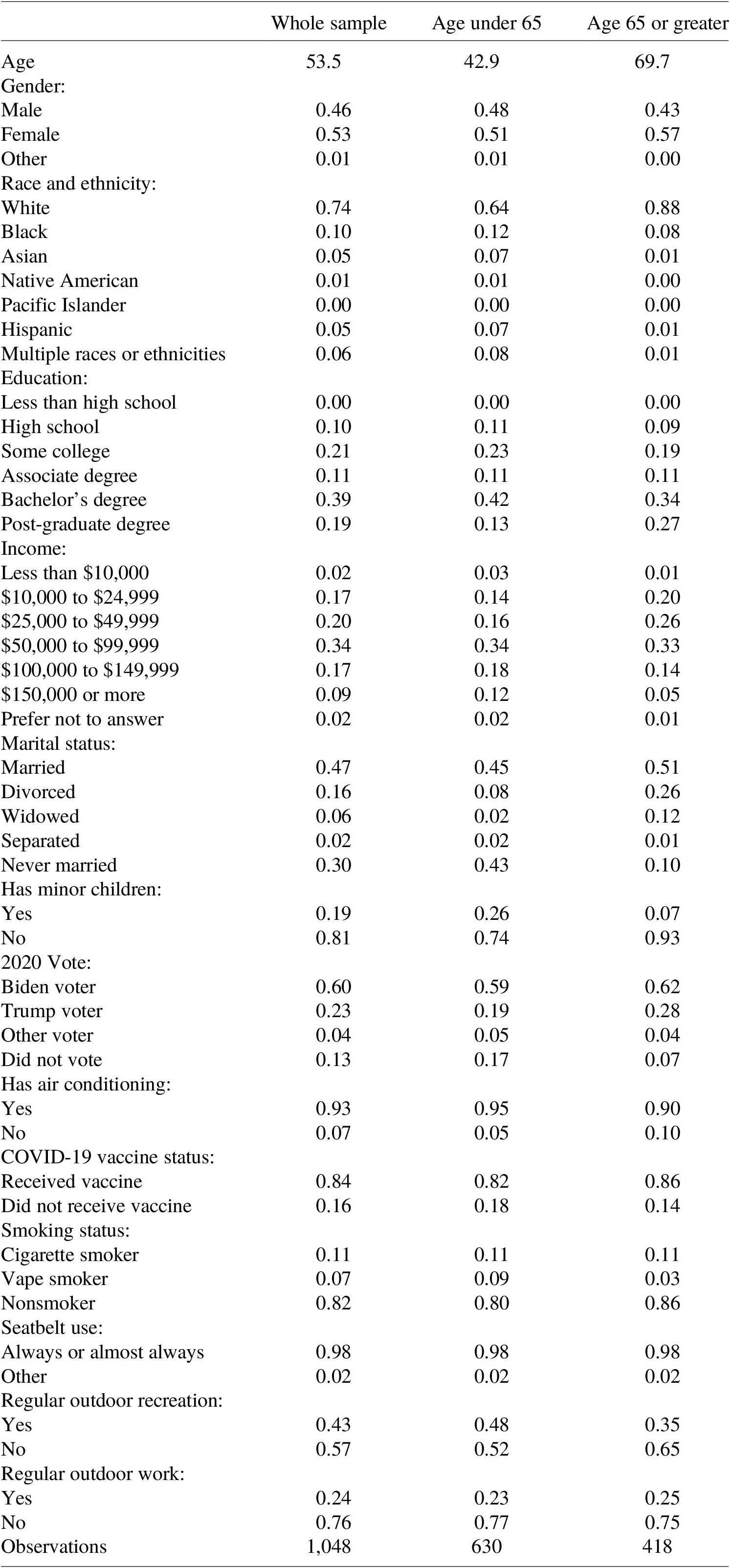
Table A2. Demographics and policy choice
Note: N = 5,240. Table reports the estimated coefficients in a multilevel logit model modeling the likelihood that respondents vote to reduce cancer or traffic deaths with reducing heat deaths as the base option. Standard errors are robust and clustered on respondent. The omitted option for sets of mutually exclusive variables is parenthetically indicated. ***p < 0.01, **p < 0.05, *p < 0.10.
Table A3. Policy choice tabulations
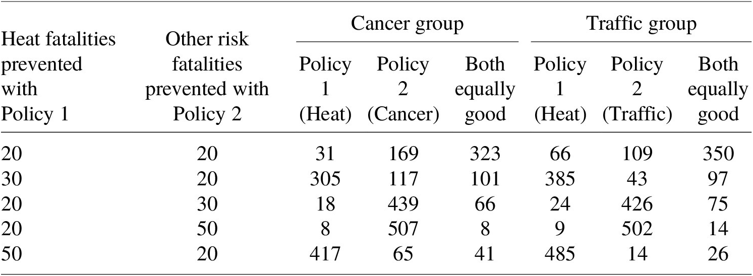
Note: Table entries indicate the number of individuals voting for Policy 1, Policy 2, or that both policies are equally good, when the number of prevented fatalities are as indicated. The cancer group contained 555 respondents, and the traffic group contained 525 respondents. Responses correspond to respondents first five policy choice questions after the attention check and warmup question.
Table A4. Policy choices tabulations when beneficiaries vary
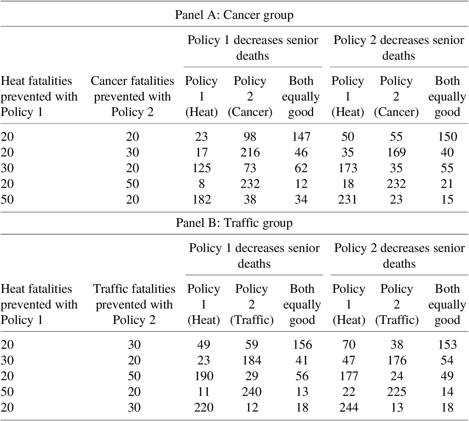
Note: Table entries indicate the number of individuals voting for Policy 1, Policy 2, or that both policies are equally good, when the number of prevented fatalities and the beneficiary of the policies are as indicated. When Policy 1 decreased senior deaths, Policy 2 decreased deaths among the general population, and vice versa. The cancer group contained 555 respondents, and the traffic group contained 525 respondents. Responses correspond to the final five policy choice questions in the questionnaire.
Online Appendix
Table A5. Policy choice regressions
Note: Table A5 reports the estimated coefficients in a conditional logit choice model modeling the likelihood that respondents vote to reduce cancer or traffic deaths with reducing heat deaths as the base option. For all risks, the omitted variable is reducing the risk by 20 deaths. Standard errors are robust and clustered on respondent. 95% confidence intervals for implied relative heat valuations are provided in brackets and calculated using the delta method. N = 15,720 for the full sample, 9,450 for the age under 65 subsample, and 6,270 for the 65 or over subsample. ***p < 0.01, **p < 0.05, *p < 0.10.
Table A6. Figure 1 regressions
Note: Table reports the estimated coefficients in conditional logit choice models modeling the likelihood that respondents vote to reduce cancer or traffic deaths with reducing heat deaths as the base option. Standard errors are robust and clustered on respondent. The sample in each column is restricted to respondents living in zip codes with average daily high temperatures over June 17–24 in 2021–2023 within 1.5 °C of the noted temperature. All coefficients in the table are statistically significant with p < 0.01.
Table A7. Figure 2 regressions

Note: Table reports the estimated coefficients in conditional logit choice models modeling the likelihood that respondents vote to reduce cancer or traffic deaths with reducing heat deaths as the base option. Standard errors are robust and clustered on respondent. The sample in each column is restricted to respondents living in zip codes with average daily high temperatures between June 17 and 24 in 2024 that deviated from historical daily average high measured in the same week in 2021–2023 by the relevant temperature plus or minus 1.5 °C. All coefficients in the table are statistically significant with p < 0.01.
Table A8. Basic policy choice regression including both equal results

Note: N=15,720. Table reports the estimated coefficients in a conditional logit choice model modeling the likelihood that respondents vote for the indicated policy, with the policy reducing heat deaths as the base option. Standard errors are robust and clustered on respondent. 95% confidence intervals for implied relative heat valuations are provided in brackets and calculated using the delta method. ***p < 0.01, **p < 0.05, *p < 0.10.
Table A9. All policy choice regressions pooled including both equal results
Note: N=31,440. Table reports the estimated coefficients in a conditional logit choice model modeling the likelihood that respondents vote for the indicated policy, with the policy reducing heat deaths as the base option. Standard errors are robust and clustered on respondent. 95% confidence intervals for implied relative heat valuations are provided in brackets and calculated using the delta method. ***p < 0.01, **p < 0.05, *p < 0.10.


 Open access