Acoustic-gravity wave triad resonance in compressible flow: a dynamical systems approach

Abstract

The classical water-wave theory often neglects water compressibility effects, assuming acoustic and gravity waves propagate independently due to their disparate spatial and temporal scales. However, nonlinear interactions can couple these wave modes, enabling energy transfer between them. This study adopts a dynamical systems approach to investigate acoustic–gravity wave triads in compressible water flow, employing phase-plane analysis to reveal complex bifurcation structures and identify steady-state resonant configurations. Through this framework, we identify specific parameter conditions that enable complete energy exchange between surface and acoustic modes, with the triad phase (also known as the dynamical phase) playing a crucial role in modulating energy transfer. Further, incorporating spatial dependencies into the triad system reveals additional dynamical effects that depend on the wave velocity and resonance conditions: we observe that travelling-wave solutions emerge, and their stability is governed by the Hamiltonian structure of the system. The phase-plane analysis shows that, for certain velocity regimes, the resonance dynamics remains similar to the spatially independent case, while in other regimes, bifurcations modify the structure of resonant interactions, influencing the efficiency of energy exchange. Additionally, modulated periodic solutions appear, exhibiting changes in wave amplitudes over time and space, with implications for wave-packet stability and energy localisation. These findings enhance the theoretical understanding of acoustic–gravity wave interactions, offering potential applications in geophysical phenomena such as oceanic microseisms.

1. Introduction

The classical theory of water waves often overlooks the impact of water compressibility, primarily because acoustic waves are typically considered to be decoupled from free-surface waves. In linear theory, this assumption is valid due to the vastly different spatial and temporal scales of acoustic propagation modes compared with free-surface waves, driven by the fact that the speed of sound in water significantly exceeds the maximum phase speed of surface waves. However, when nonlinear wave interactions are considered, neglecting compressibility may no longer be justified. Longuet-Higgins (1950) highlighted this in a seminal paper, demonstrating that quadratic interactions of gravity surface waves can resonantly excite compression modes in finite-depth water. He proposed that this nonlinear coupling mechanism is crucial for generating oceanic microseisms – small oscillations of the seafloor in the frequency range of 0.1–0.3 Hz.

Longuet-Higgins (1950) focused on a scenario where two oppositely propagating gravity wavetrains of the same frequency decay exponentially with depth, consistent with classical, incompressible water-wave theory. At the second order, however, quadratic interactions produce a space-averaged pressure component at twice the wave frequency, which does not attenuate with depth. When the water depth is comparable to the acoustic wavelength, compressibility must be considered to accurately compute the induced pressure disturbance within the fluid. Accounting for compressibility, the second-order response shows a resonance when a free compression mode has twice the surface-wave frequency, suggesting optimal conditions for microseism generation, as supported by recent North Atlantic field observations (Kedar et al. 2008).

Building on this, Kadri & Stiassnie (2013) provided numerical evidence that the resonances identified by Longuet-Higgins (1950) are specific instances of resonant wave triads involving a propagating acoustic wave mode and two oppositely travelling subharmonic surface waves. They further argued that these resonant acoustic–gravity interactions are described by amplitude equations similar to those of a standard resonant triad (Bretherton 1964).

Subsequently, Kadri & Akylas (2016) analysed triads consisting of a long-crested acoustic mode and two oppositely propagating subharmonic gravity waves. Due to the significant difference in the scales of gravity and acoustic waves, the interaction time scale is longer than that of a standard resonant triad, and the amplitude evolution equations include certain cubic terms in addition to the usual quadratic interaction terms. Despite this complexity, finely tuned triads can form, and it was shown that nearly all the energy initially in the gravity waves may transfer to the acoustic mode. However, this energy transfer mechanism is significantly less effective for locally confined wave packets.

In this study, we adopt a dynamical systems approach to further explore the results obtained by Kadri & Akylas (2016). The key emergent degrees of freedom in this approach are the so-called triad phases, or dynamical phases (Bustamante & Kartashova 2009; Harris, Bustamante & Connaughton 2012), whose dynamical evolution and synchronisation can influence strongly the way energy is transferred across different modes, as shown in a variety of physical scenarios: generation of low-frequency Rossby waves in the atmosphere (Raphaldini et al. 2022), long-term solar cycles in magnetohydrodynamic Rossby waves (Raphaldini et al. 2019), turbulence in one-dimensional compressible flows (Buzzicotti et al. 2016; Murray & Bustamante 2018; Arguedas-Leiva et al. 2022; Protas, Kang & Bustamante 2024), type I and type II instabilities of surface gravity waves (Andrade & Stuhlmeier 2023b , c ; Heffernan, Chabchoub & Stuhlmeier 2024), dissipation events and turbulence in two- and three-dimensional incompressible flows (Bustamante, Quinn & Lucas 2014; Walsh & Bustamante 2020; Redfern, Lazer & Lucas 2024; Wang et al. 2024). Utilising phase-plane analysis, in the current work we examine the solutions on separatrices, revealing rich structure and a variety of bifurcations. Fixed points in the interior of the phase space are identified with steady-state resonant triads first found by Yang, Dias & Liao (2018). We find that specific values of detuning parameter $\gamma$ allow for full asymptotic energy exchange between surface and acoustic–gravity modes. At the same time, we see how the triad phase, constructed as a kind of phase difference from surface and acoustic modes, can increase or decrease energy exchange, which may be important for practical applications.

2. Preliminaries

Consider the propagation of surface–acoustic wave disturbances in water of constant depth $h$ over a rigid bottom ( $z=-h$ ), due to the combined action of gravity and compressibility. Water will be treated as an inviscid, barotropic fluid (where the pressure $p$ is a function of the density $\rho$ only) with constant sound speed $c=(\textrm {d} p/\textrm {d} \rho)^{1/2}$ , and the motion will be assumed irrotational. A key parameter, which controls the effects of compressibility relative to gravity, is

(2.1) \begin{align} \mu = \frac {gh}{c^2}, \qquad (\mu \ll 1), \end{align}

where $g$ is the gravitational acceleration. Typically, this parameter is small ( $\mu \ll 1$ ), as the sound speed in water, $c=1.5\times 10^3$ m s^–1, far exceeds the maximum gravity-wave phase speed $(gh)^{1/2}$ (under oceanic conditions, for $h=150$ – $1500$ m, say, $\mu \simeq 10^{-3}$ – $10^{-2}$ ). As a result, free-surface (gravity) wave disturbances feature vastly different spatial and/or temporal scales from acoustic (compression) wave modes.

Assuming irrotational flow, the surface–acoustic wave problem is formulated in terms of the velocity potential $\varphi (x,z,t)$ , where $\mathbf{u}=\nabla \varphi$ is the velocity field. Moreover, we shall use dimensionless variables, employing $\unicode{x03BC} h$ as length scale and $h/c$ as time scale. As in Longuet-Higgins (1950), the equation governing $\varphi$ in the fluid interior is obtained by combining continuity with the unsteady Bernoulli equation. Specifically, $\varphi$ satisfies

(2.2) \begin{align} \frac {1}{\mu ^2}\left (\varphi _{xx}+\varphi _{zz}\right)-\varphi _{tt}-\varphi _z-|\nabla \varphi |^2_t-\frac {1}{2}\mathbf{u}\cdot \nabla \left (|\nabla \varphi |^2\right)=0, \end{align}

with the combined (kinematic and dynamic) condition on the free surface

(2.3a) \begin{align} \begin{aligned} \varphi _{tt}+\varphi _z +|\nabla \varphi |^2_t - \{\varphi _t\left (\varphi _{tt}+\varphi _z\right) \}_z +\frac {1}{2}\mathbf{u}\cdot \nabla \left (|\nabla \varphi |^2\right) -\big \{\varphi _t |\nabla \varphi |^2_t\big \}_z\\ -\frac {1}{2} \Big \{\left (\varphi _{tt}+\varphi _z\right) \left (|\nabla \varphi |^2 - \varphi _t^2\right)\Big \}_z=0 \qquad (z=0), \end{aligned} \end{align}

and the boundary condition on the rigid bottom at $z=-1/\mu$ reads

(2.3b) \begin{align} \varphi _{z}=0 \qquad (z=-1/\mu). \end{align}

In the limit $\mu \ll 1$ , equation (2.2) along with the boundary conditions (2.3) reduce to the classical incompressible deep-water wave problem (correct to cubic terms). This reflects the fact that the chosen length scale $\mu h$ pertains to deep-water gravity waves, which are confined close to the free surface. Acoustic waves, by contrast, extend through the entire fluid depth, and $x$ and $z$ have to be re-scaled accordingly in order to capture these disturbances for $\mu \ll 1$ .

For the gravity wave, the frequency $\omega$ satisfies the dispersion relation

(2.4) \begin{align} \omega ^2=|k|+O(\mu ^4), \end{align}

where $k$ is the wavenumber.

For the acoustic modes there is a countable infinity of propagation modes which obey the dispersion relations

(2.5) \begin{align} \omega ^2=\omega _n^2+\kappa ^2+\mu \frac {\omega _n^2-\kappa ^2}{\omega _n^2+\kappa ^2}+O(\mu ^2)\qquad (n=0,1,2,\ldots), \end{align}

where $\omega _n \equiv (n+({1}/{2}))\pi$ .

Consider two gravity waves $(k_+,\omega _+)$ and $(k_-,\omega _-)$ observing the dispersion relation (2.4), along with an acoustic wave $(\mu \kappa,\omega)$ which satisfies the dispersion relations (2.5) for some $n=0,1,2,\dots$ . To form a resonant triad, these modes must also obey the resonance conditions

(2.6) \begin{align} \textrm {(i)}\quad k_++k_-=\mu \kappa; \qquad \textrm {(ii)}\quad \omega _++\omega _-=\omega. \end{align}

3. Resonant wave triads: dynamics and evolution

For a slow time scale $T=\mu t$ , the amplitude evolution equations for the acoustic mode $A(T)$ and the two gravity waves $S_{\pm }(T)$ are given by (Kadri & Akylas 2016)

(3.1) \begin{align} \frac {\textrm {d} A}{\textrm {d} T} = \textrm {i}\gamma A + \delta S_+S_-, \end{align}

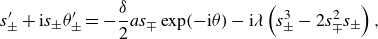
(3.2) \begin{align} \frac {\textrm {d} S_{\pm }}{\textrm {d} T} = -\frac {\delta }{2}AS^*_{\mp }- i \lambda \left ({{S_{\pm }}}^2S^*_{\pm } - 2|S_{\mp }|^2S_{\pm }\right), \end{align}

where

(3.3) \begin{align} \gamma \equiv \frac {\kappa ^2-\omega _n^2}{2\omega ^3}-\beta; \quad \delta \equiv \frac {(-1)^n}{4} \omega _n \omega ^2 \alpha; \quad \lambda \equiv \frac {1}{64}\omega ^7 \alpha ^2, \end{align}

and $*$ stands for complex conjugate. The terms on the right-hand side of (3.2) account for the quadratic and cubic interactions, which enter the evolution equations at the same order for $\alpha =O(1)$ , $\beta$ is the detuning introduced in (Kadri & Akylas 2016, Eq. (5.2)), such that $\gamma$ is a measure for the overall resonance detuning, which we call the detuning parameter.

Writing the variables in terms of complex exponentials $A = a\exp (\textrm {i}\theta _a)$ and $S_\pm = s_\pm \exp (\textrm {i}\theta _\pm),$ where both the amplitudes $a, \, s_{\pm }$ and the phases $\theta _a, \, \theta _{\pm }$ are unknown functions of time, allows us to split the triad resonance system into the following:

(3.4) \begin{align} a^{\prime} + \textrm {i} a \theta _a^{\prime} = \textrm {i} \gamma a + \delta s_+ s_- \exp (\textrm {i}\theta), \end{align}

(3.5) \begin{align} s_\pm ^{\prime} + \textrm {i} s_\pm \theta _\pm ^{\prime} = -\frac {\delta }{2}a s_\mp \exp (-\textrm {i}\theta) - \textrm {i} \lambda \left ( s_\pm ^3 - 2 s_\mp ^2 s_\pm \right), \end{align}

where we have introduced the triad phase or dynamical phase $\theta \equiv \theta _+ + \theta _- - \theta _a$ (Bustamante & Kartashova 2009). The key insight that the three individual phases $\theta _a, \ \theta _{\pm }$ do not influence the resonant interaction except in this single combination is the first step to reducing the dimension of the resulting system.

Separating (3.4)–(3.5) into real and imaginary parts results in the system

(3.6) \begin{align} a^{\prime} = \delta s_+ s_- \cos (\theta); \quad s_\pm ^{\prime} = -\frac {\delta }{2}a s_\mp \cos (\theta), \end{align}

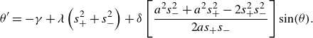(3.7) \begin{align} \theta ^{\prime} = -\gamma + \lambda \left ( s_+^2 + s_-^2 \right) + \delta \left [ \frac {a^2 s_-^2 + a^2 s_+^2 - 2 s_+^2 s_-^2}{2as_+s_-}\right]\sin (\theta). \end{align}

The two conserved quantities for this system, $W$ and $K,$ identified with the total energy and surface-wave energy difference. Judicious use of these will allow us to eliminate two of the three amplitudes, and recast our equations in the phase plane. These conserved quantities can be written compactly as

(3.8) \begin{align} \begin{pmatrix} 1 & 1 & 1\\ 0 & 1 & -1 \end{pmatrix} \begin{pmatrix} a^2 \\ s_+^2 \\[4pt] s_-^2 \end{pmatrix} = \begin{pmatrix} W \\ K \end{pmatrix}, \end{align}

where we take $K \geqslant 0$ without loss of generality. This system has the following general solution, in terms of the single unknown function $\eta (t)$ :

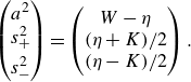(3.9) \begin{align} \begin{pmatrix} a^2\\s_+^2\\[4pt] s_-^2 \end{pmatrix} = \begin{pmatrix} W-\eta \\ (\eta +K)/{2} \\ (\eta -K)/{2} \end{pmatrix}. \end{align}

Substitution of the solution allows us to write the triad system in terms of two variables

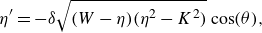(3.10) \begin{align} \eta ^{\prime} = {-\delta } \sqrt {(W-\eta)(\eta ^2 - K^2)} \cos (\theta), \end{align}

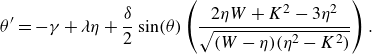(3.11) \begin{align} \theta ^{\prime} = -\gamma + \lambda \eta + \frac {\delta }{2} \sin (\theta) \left ( \frac {2\eta W + K^2 -3 \eta ^2}{\sqrt {(W-\eta)(\eta ^2-K^2)}} \right). \end{align}

Integration of these equations yields immediately the Hamiltonian

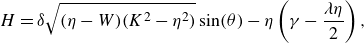(3.12) \begin{align} H = {\delta } \sqrt {(\eta - W)(K^2 - \eta ^2)} \sin (\theta) - \eta \left (\gamma - \frac {\lambda \eta }{2}\right), \end{align}

with

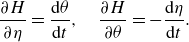(3.13) \begin{align} \frac {\partial H}{\partial \eta } = \frac {\textrm {d} \theta }{\textrm {d} t}, \quad \frac {\partial H}{\partial \theta } = -\frac {\textrm {d} \eta }{\textrm {d} t}. \end{align}

Note that the two-dimensional, Hamiltonian system (3.10)–(3.11) is entirely equivalent to the original system of three complex equations (3.1)–(3.2). The simpler system obtained by Kadri & Stiassnie (2013) can likewise be cast in Hamiltonian form by setting $\lambda =0$ and $\gamma =0,$ thereby eliminating the cubic terms and the detuning, respectively.

The Hamiltonian $H$ has Jacobi matrix

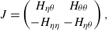(3.14) \begin{align} J = \begin{pmatrix} {H}_{\eta \theta } & {H}_{\theta \theta } \\[3pt] -{H}_{\eta \eta } & -{H}_{\eta \theta } \end{pmatrix}, \end{align}

with determinant $\det (J) = {H}_{\theta \theta } {H}_{\eta \eta } - {H}^2_{\eta \theta }.$ At a fixed point of the system, the eigenvalues corresponding to the linearised solution are $\lambda _{1,2} = \pm \sqrt {-\det (J)}.$

This approach of reducing wave interaction equations to a dynamical system has been previously employed for cubically nonlinear three-wave mixing in optical fibres by Cappellini & Trillo (1991), and has recently been used to explore several classical instabilities for free-surface water waves (see e.g. Andrade & Stuhlmeier 2023b ). We shall see that it readily yields a new and transparent view of the acoustic–gravity wave resonance problem.

4. Phase-plane analysis

The principal advantage of reducing the three complex resonant interaction equations (3.1)–(3.2) to a (real-valued) planar Hamiltonian system (3.10)–(3.11) is in allowing simple insight via phase-plane analysis. The single dynamical phase (sometimes termed triad phase in this context) $\theta$ and energy parameter $\eta$ allow the problem to be formulated in a domain $(\eta,\theta)\in (K,W)\times [-\pi,\pi]$ (recall that $K\geqslant 0$ without loss of generality, and $W\gt K$ by (3.9)). As $\eta$ tends to the lower limit of the energy scale $\eta =K$ we have a system consisting of the acoustic mode $a$ and one surface mode $s_+,$ while at the upper limit $\eta =W$ we have two surface modes $s_-$ and $s_+$ only (see (3.9)). When surface mode energy is equipartitioned, $K=0$ , and the lower limit corresponds to the acoustic mode $a$ only. This points to a significant difference between cases with ( $K=0$ ) and without ( $K\neq 0$ ) such equipartition.

We begin the phase-plane analysis by identifying nullclines and fixed points of the system. By straightforward inspection the nullclines of (3.10) are $\eta = W$ , $\eta = K$ and $\theta = \pm \pi /2.$ Meanwhile, we can obtain the nullcline of (3.11) by setting the right-hand side equal to zero, i.e.

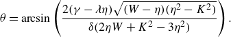(4.1) \begin{align} \theta = \arcsin \left ( \frac {2 (\gamma -\lambda \eta)\sqrt {(W-\eta)(\eta ^2-K^2)}}{\delta (2\eta W + K^2 - 3 \eta ^2)} \right). \end{align}

We note that, as $\eta \rightarrow W,$ the nullcline intersects the points $(\eta,\theta)=(W,0)$ and $(W,\pm \pi).$ Consequently there are always fixed points of the system (3.10)–(3.11) at the top of the phase plane. If $K\neq 0$ the same holds as $\eta \rightarrow K,$ i.e. as we approach the bottom of the phase plane. In this case we always have fixed points in these positions, limiting the types of bifurcation that can take place. On the other hand, for $K=0,$ i.e. equipartition of energy between the two surface waves, we can find fixed points at the bottom of the phase plane with

(4.2) \begin{align} \theta =\arcsin \! \left (\frac {\gamma }{\delta \sqrt {W}}\right),\end{align}

when the argument of arcsin is of magnitude less than or equal to 1.

We can also establish the existence of an interior fixed point along the nullcline of $\eta$ corresponding to $\theta = \pm \pi /2.$ For $\theta =\pi /2$ setting the right-hand side of (3.11) to zero yields

(4.3) \begin{align} p(\eta) \equiv \left (\gamma - \lambda \eta \right){\sqrt {(W-\eta)(\eta ^2-K^2)}} - \frac {\delta }{2} \left ( 2\eta W + K^2 -3 \eta ^2 \right). \end{align}

Evaluating at the limits $\eta =K$ and $\eta =W$ gives

(4.4) \begin{align} p(K)=\delta K(W-K), \qquad p(W) = \frac {\delta }{2}(K^2-W^2), \end{align}

which have opposite signs when $K \neq 0$ , implying the existence of a zero. The same argument is true for $\theta =-\pi /2.$

4.1. Bifurcation with equal surface-wave amplitudes

When the surface-wave amplitudes are equal four parameters remain in our problem: the total energy $W$ (see (3.9)), the modal parameter $\delta$ (which depends on the acoustic–gravity mode and frequencies considered), the steepness parameter $\alpha$ and the detuning $\gamma.$ As the lowest acoustic–gravity mode is dominant, and following the work of Kadri & Akylas (2016) we will take $n=0$ and $\omega _0=\pi /2$ as well as $\omega =\sqrt {1+\pi ^2/4}$ in all subsequent examples. Taking $\alpha =1$ then fixes $\delta$ via (3.3). If we subsequently choose the total energy $W=2$ (see (Kadri & Akylas 2016, (6.1))) this leaves the detuning $\gamma$ as a bifurcation parameter for our system.

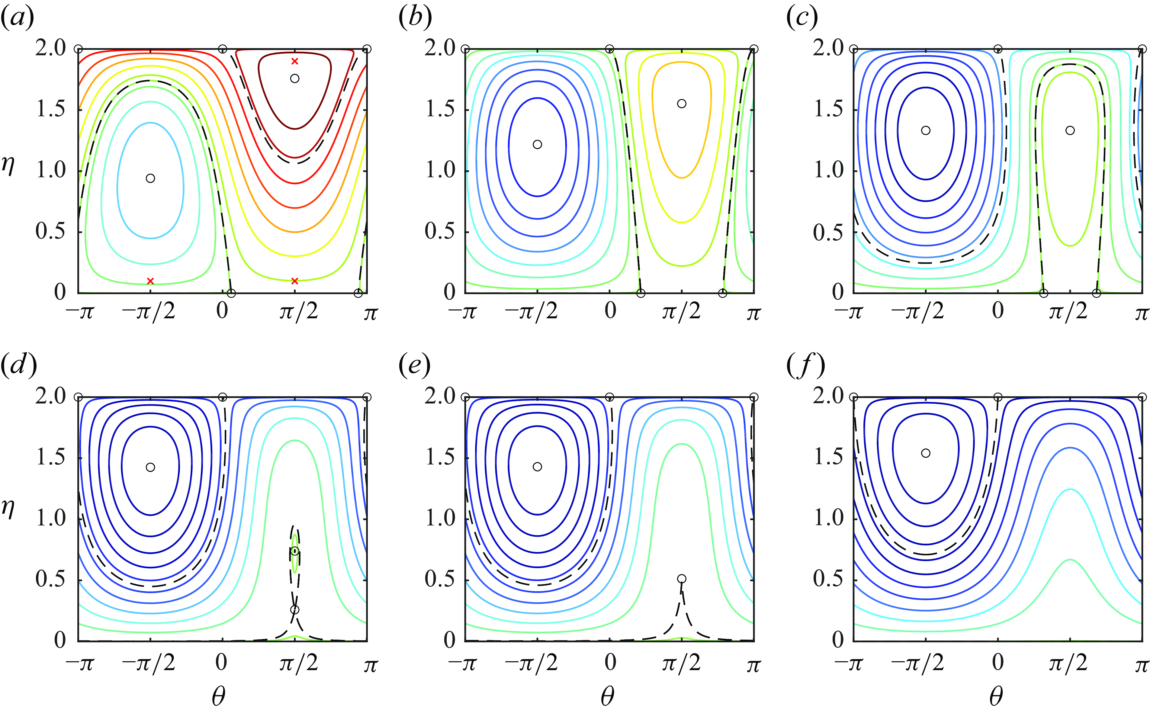
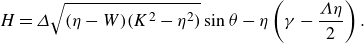
Figure 1. Characteristic phase portraits for $K=0,$ $W=2$ and $\alpha =1$ for various values of detuning parameter. Panels show $\gamma = 0.36$ (a), $\gamma =\lambda W/2 \approx 1.21$ (b), $\gamma \approx 1.62$ (c), $\gamma \approx 1.98$ (d), $\gamma \approx 1.20$ (e) and $\gamma = 2.5$ (f). Each curve is a level line of the Hamiltonian, so that trajectories of the system in $(\eta,\theta)$ remain confined to these level lines; fixed points are denoted by circles ( $\bigcirc$ ), and separatrices connecting these fixed points are denoted by dashed, black curves. For the interpretation of the red $\times$ s in panel (a) refer to figure 2.

Figure 1 shows six characteristic phase portraits for a fixed value of $\alpha =1,$ with various values of detuning parameter $\gamma$ . Trajectories are level lines of the Hamiltonian (3.12), with colours denoting the value of the Hamiltonian. Fixed points are denoted by circles, while separatrices are shown as dashed black lines. For sufficiently small (negative) values of detuning $\gamma,$ condition (4.2) is violated and no fixed points occur at $\eta = 0$ (not shown). Fixed points appear at $\eta =0$ when $\gamma =\pm \delta \sqrt {W},$ at which point a bifurcation splits the fixed point at $(\eta,\theta)=(0,\pm \pi /2)$ into the two fixed points $(\eta,\theta)=(0,\arcsin (\pm \gamma \delta ^{-1} W^{-1/2}))$ seen in panels (a)–(c).

Still referring to figure 1, for sufficiently small steepness $\alpha \leqslant {32 \omega _{n}}\omega ^{-5}W^{-1/2}$ and $\gamma =\lambda W/2$ (shown in panel (b)) separatrices connecting fixed points at the top and bottom of the domain merge – the solution along this separatrix exhibits total conversion as two surface modes are asymptotically converted into an acoustic mode or vice versa. This corresponds to the ‘perfectly tuned’ situation discussed by (Kadri & Akylas 2016, Section 6), and describes a departure from the prototypical cyclic energy exchange seen elsewhere in the phase plane.

As the detuning parameter $\gamma$ increases further, the fixed points at $\eta = 0$ undergo a saddle-node bifurcation (panel (d)), where they coalesce and then vanish. This is followed by a centre-saddle bifurcation (panel (e)), characterised by the disappearance of the remaining fixed points due to the vanishing discriminant of the cubic polynomial

(4.5) \begin{align} q(\eta) = 4 (\gamma - \lambda \eta)^2 (W - \eta) - \delta ^2 (2W - 3\eta)^2. \end{align}

It is instructive to move from the phase space shown in figure 1 to the time evolution of the physical mode amplitudes. This is the natural setting for the original system of interaction equations (3.1)–(3.2). We shall visualise the modal interactions for $\alpha =1$ and detuning parameter $\gamma = 0.36,$ as shown in figure 1, panel (a). As initial conditions we employ the values of energy distribution and dynamic phase given at the three red $\times$ symbols in the aforementioned panel: $\eta (0)=0.1, \, \theta (0)=-\pi /2,$ $\eta (0)=0.1, \, \theta (0)=\pi /2$ and $\eta (0)=W-0.1, \, \theta (0)=\pi /2.$

These three initial conditions belong to different parts of the phase space separated by the separatrices (dashed black curves in figure 1): these are orbits surrounding the centre at $\theta =-\pi /2,$ orbits surrounding the centre at $\theta =\pi /2$ and trajectories between the two separatrices. The first two domains are characterised by a confined dynamical phase, and are depicted in panel (a) and panel (c) of figure 2, respectively. The last is shown in panel (b) of figure 2, where the dynamical phase is wrapped to $[-\pi,\pi].$

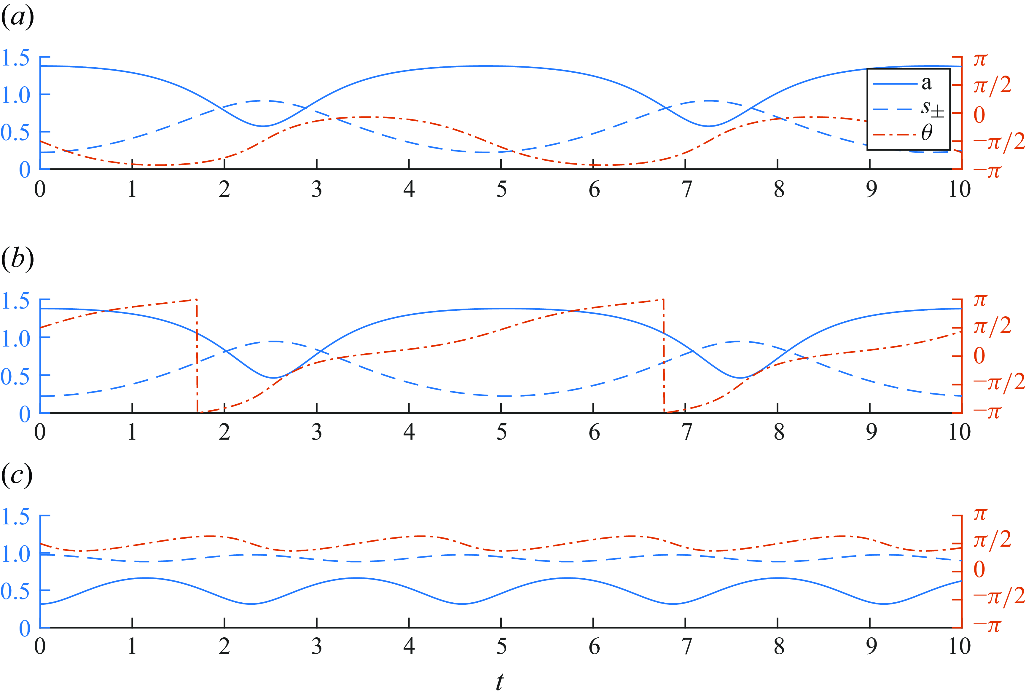
Figure 2. Resonant interaction throughout the phase space for $K=0$ and $\gamma = 0.36$ (Panel (a), figure 1) corresponding to the initial conditions shown as red $\times$ symbols in figure 1. Left axes show the amplitudes of surface (dashed blue curves) and acoustic modes (solid blue curves). Right axes show the dynamical phase (dash-dotted red curves). Panel (a) $\eta (0)=0.1, \, \theta (0)=-\pi /2.$ Panel (b) $\eta (0)=0.1, \, \theta (0)=\pi /2.$ Panel (c) $\eta (0)=W-0.1, \, \theta (0)=\pi /2.$ .

In the phase-plane description, the energy exchange among the acoustic mode $a$ and the surface modes $s_\pm$ is given by the excursion of $\eta$ along a given contour. For instance, if an additional panel were added to figure 2 showing initial data at an interior fixed point, the result would depict three horizontal lines, corresponding to a steady-state resonance. The trajectories confined around the fixed point at $\theta =\pi /2$ in figure 1(a) demonstrate only limited energy exchange over time, as shown in figure 2(c). Both representations of the resonant interaction illustrate that the greatest energy exchange (maximum of $\eta ^{\prime}$ ) along a contour occurs when there is minimal variation in the dynamical phase (minimum of $\theta ^{\prime}$ ), and vice versa. A detailed exploration of the conditions for optimal energy conversion between acoustic and surface modes will follow in subsequent sections.

4.2. Fixed points as steady-state triads

The interior fixed points we find are steady-state resonant acoustic–gravity triads, which have previously been discovered in isolation using the homotopy analysis method (HAM) by Yang et al. (2018). Their high-order, iterative procedure yields such steady states in the context of triads without detuning and in the absence of cubic terms, which amounts to setting both $\gamma$ and $\lambda$ to zero in (3.10)–(3.11).

The phase-plane analysis we undertake shows that such steady states are ubiquitous in the acoustic–gravity wave interaction. Indeed, making the substitution $\gamma =\lambda =0$ in (3.11) shows that interior fixed points are always centres, and exist independent of mode number or other parameters. For any values of $W$ and $K$ they are located at $(\eta,\theta)=( (W+\sqrt {3K^2+W^2})/3,\pm {\pi }/{2})$ . Although Yang et al. (2018) do not report the phases of their steady-state solutions, it is easy to verify that their iteration converges to amplitudes partitioned as per $\eta$ above, i.e. using $\eta =W-a^2$ and given values of $K$ and $W.$ The agreement is not exact, since their high-order expansion allows for energy to exist in wave modes other than $a, s_+$ and $s_-$ , whereas we are strictly confined to three modes only.

4.3. Bifurcation with unequal surface-wave amplitudes

When the two surface modes have unequal amplitudes, complete asymptotic conversion of all surface-wave energy into an acoustic mode is not possible. This limitation arises because the phase space depends on the conserved energy difference $K$ . Consequently, in addition to specifying total energy $W$ and other parameters as outlined in § 4.1, the value of $K$ must also be defined. Using $n=0$ and the values of $\omega _0, \, \omega$ from § 4.1, we select $W=2,$ $K=0.1$ and $\alpha =1.2.$

Non-symmetric surface waves imply the existence of fixed points at $\theta =0, \pm \pi$ at both the top and bottom of the phase space. However, variations of the detuning $\gamma$ give rise to bifurcations, much as in the symmetric case discussed above. Indeed, as $\gamma$ is increased to $\gamma = \lambda (K+W)/2,$ we find that separatrices connect the two boundaries of the phase plane, as depicted in figure 3(b). This represents asymptotic conversion of two surface modes with $s_\pm ^2 = (W\pm K)/2$ into one surface mode with $a^2=W-K$ and one acoustic mode with $s_+^2 = K$ , or vice versa (see (3.9)).

Figure 3. Characteristic phase portraits for $K=0.1,$ $W=2$ and $\alpha =1.2$ for various values of increasing detuning parameter. Panels show $\gamma = -0.55$ (a), $\gamma = \lambda (K+W)/2 \approx 1.83$ (b), $\gamma =2.2$ (c), $\gamma \approx 2.58$ (d), $\gamma \approx 2.60$ (e) and $\gamma =3.50$ (f). Each curve is a level line of the Hamiltonian, so that trajectories of the system in $(\eta,\theta)$ remain confined to these level lines; fixed points are denoted by circles ( $\bigcirc$ ), and separatrices connecting these fixed points are denoted by dashed, black curves.

As $\gamma$ continues to increase, a pitchfork bifurcation emerges (illustrated in panels (d) and (e) of figure 3), producing two centres and a saddle point from the single centre initially located at $\theta =\pi /2$ in panels (a)–(c). This bifurcation occurs for specific values of $K$ , $W$ and $\alpha$ , such that the quintic derived from (3.11) at $\theta =\pi /2$ possesses three real roots within the interval $[K,W]$ . As the detuning parameter $\gamma$ increases, fixed points at the boundaries remain present (cf. panel (f) in figures 1 and 3), but the qualitative behaviour remains similar: large detuning, whether positive or negative, results in a flattening of orbits, signifying reduced energy exchange among the modes.

4.4. Optimal energy conversion

From a physical perspective, the most intriguing solutions revealed through phase-plane analysis are those enabling the asymptotic conversion of all energy. This occurs either from two surface modes into a single acoustic mode (when $K=0$ ) or from two surface modes into one acoustic and one surface mode (when $K\neq 0$ ). Remarkably, these solutions can be computed analytically.

For given values of $W$ and $K$ , maximal energy exchange is observed along a separatrix that connects the top ( $\eta = W$ ) and bottom ( $\eta = K$ ) boundaries of the domain. A necessary condition for the existence of such a particular solution is that the values of the Hamiltonian at $\eta = W$ and $\eta = K$ are equal, expressed as

(4.6) \begin{align} H(W,\theta) = -W\left (\gamma - \frac {\lambda W}{2}\right) = -K\left (\gamma - \frac {\lambda K}{2}\right) = H(K,\theta), \end{align}

which amounts to choosing $\gamma = {\lambda }(W + K)/2$ . For this specific choice of $\gamma$ , the existence of a separatrix requires

(4.7) \begin{align} \delta \sqrt {(W - \eta)(\eta ^2 - K^2)}\sin (\theta) = -\frac {\lambda }{2}(\eta - K)(\eta - W). \end{align}

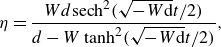
This allows us to simplify (3.10) considerably, squaring it and substituting the above to obtain

(4.8) \begin{align} (\eta ^{\prime})^2 = (W - \eta)(\eta - K)\left (\delta ^2(\eta + K) - \frac {\lambda ^2}{4}(\eta - K)(W - \eta)\right)= P_4(\eta). \end{align}

Here, $P_4(\eta)$ is a degree-4 polynomial in $\eta$ , and so equation (4.8) can be solved exactly by means of elliptic functions. We compute the separatrix explicitly for $K = 0$ . The equation that needs to be solved in this case is a simplification of (4.8)

(4.9) \begin{align} (\eta ^{\prime})^2 = (W - \eta)\eta ^2\left (\frac {\lambda ^2}{4}\eta + \delta ^2 - \frac {\lambda ^2}{4}W\right). \end{align}

The roots of the polynomial are $W$ and $0$ (with multiplicity two) and $d = W - 4{\delta ^2}/{\lambda ^2}$ which is negative whenever fixed points at $\eta = 0$ exist. The solution of equation (4.9) can be obtained through separation of variables, yielding

(4.10) \begin{align} \tanh ^{-1}\left (\sqrt {\frac {d(\eta - W)}{W(\eta - d)}}\right) = \frac {\sqrt {-Wd}}{2}t. \end{align}

Here, it is important to note that $d\leqslant 0$ , and this expression is valid only for $t\geqslant 0$ , as the argument of the hyperbolic tangent must remain non-negative. Thus, the solution to the differential equation is given by

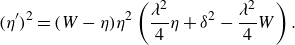
(4.11) \begin{align} \eta = \frac {Wd\textrm {sech}^2(\sqrt {-W{\rm d}}t/2)}{d - W \tanh ^2(\sqrt {-W{\rm d}}t/2)}, \end{align}

valid for $t\geqslant 0$ only. Additionally, note that $\eta (0) = W$ , meaning the solution starts at the upper boundary and progressively approaches the lower boundary of the domain. This represents the optimal configuration, where the gravity-wave transfers all its energy to the acoustic mode.

Once $\eta$ is determined, $\theta$ can be calculated using (4.7). Employing the same parameter values as those used in § 4.1, figure 4 illustrates the solution along the separatrix originating from $\eta (0)=W$ and $\theta (0)=0$ , as depicted in panel (b) of figure 1.

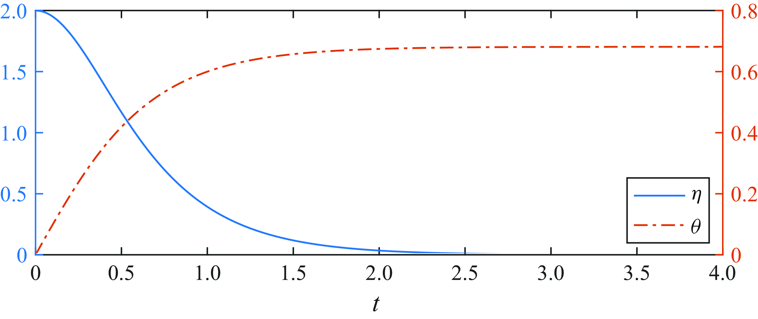
Figure 4. Optimal energy conversion along the separatrix shown in figure 1(b).

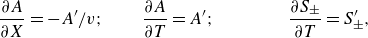
5. Spatial dependency

For the more general wave-packet resonant interaction, the wave envelopes $A$ and $S_\pm$ display spatio-temporal modulations. For $\kappa =O(1)$ , the appropriate spatial envelope variable is $X=\mu ^2 x$ . In this setting only the acoustic amplitude equation is modified, to the following:

(5.1) \begin{align} \frac {\partial A}{\partial T} +\frac {\kappa }{\omega }\frac {\partial A}{\partial X}={\textrm {i}}\gamma A+\delta S_+S_-, \end{align}

whereas the evolution equation for the gravity modes remains unchanged, except for a parametric spatial dependency (see Kadri & Akylas 2016), namely the above equation is combined with (3.2). Notice that now the general problem is to look for a solution of the system of (5.1), (3.2) such that $A, S_+$ and $S_-$ are functions of $X$ and $T$ .

5.1. Travelling-wave solution with velocity $v$

While pursuing a general solution to such a system is an intriguing endeavour, likely connected to the theory of integrable systems (Calogero & Degasperis 2004; Degasperis & Lombardo 2007), here, attention is focused on gaining insights by examining specific solutions. We assume that $A$ and $S_\pm$ are functions of the real variable $\xi \equiv T - X/v$ , where $v\neq 0$ . This represents a fixed ‘profile’ propagating at a constant velocity $v$ in the $X$ -direction. Although the profile is fixed, it is non-trivial, with its shape governed by the nonlinear interaction between $A$ and $S_\pm$ , as demonstrated below.

Assuming $A=A(T-X/v)$ and $S_\pm = S_\pm (T-X/v)$ , and denoting the derivative of a function with respect to its argument by a prime, we have

(5.2) \begin{align} \frac {\partial A}{\partial X} = -A^{\prime}/v; \qquad \frac {\partial A}{\partial T} = A^{\prime}; \qquad \qquad \frac {\partial S_\pm }{\partial T} = S_\pm ^{\prime}, \end{align}

where we have omitted the argument $\xi = T-X/v$ of the above functions. Replacing the above into (5.1), (3.2) we obtain the system

(5.3) \begin{align} \left (1-\frac {\kappa }{\omega v}\right)A^{\prime} = \textrm {i}\gamma A+\delta S_+ S_-; \qquad S_{\pm }^{\prime} = -{\frac {\delta }{2}} AS_{\mp }^*-\textrm {i}\lambda \left (S_{\pm }^2S_{\pm }^*-{ 2}|S_{\mp }|^2S_{\pm }\right). \end{align}

The analysis is divided into two cases for $v\neq 0$ : (i) $v={\kappa }/{\omega }$ , and (ii) $ v \neq {\kappa }/{\omega }$ . In case (i) the system simplifies as follows:

(5.4) \begin{align} A = \textrm {i}\frac {\delta }{\gamma } S_+ S_-; \qquad S_{\pm }^{\prime}= -\textrm {i}\left (\lambda |S_{\pm }|^2+\left ({\frac {\delta ^2}{2 \gamma }} -{2\lambda }\right)|S_{\mp }|^2\right)S_{\pm }. \end{align}

In this case the dynamics simplifies considerably, yielding the general solution

(5.5) \begin{align}\begin{aligned} A(\xi) &= \textrm {i}\frac {\delta }{\gamma } M_+ M_- \exp (-\textrm {i} (\Omega _+ + \Omega _-)\xi + \textrm {i} (\Phi _+ + \Phi _-)); \\ S_\pm (\xi) &= M_\pm \exp (-\textrm {i} \Omega _\pm \xi + \textrm {i} \Phi _\pm), \end{aligned}\end{align}

where

(5.6) \begin{align} \Omega _\pm \equiv {\lambda }M_{\pm }^2+\left ({\frac {\delta ^2}{2 \gamma }} -{2\lambda }\right)M_{\mp }^2. \end{align}

Here, $M_\pm$ are arbitrary non-negative constants, and $\Phi _\pm$ are arbitrary real constants. Notably, this solution introduces phase modulation while leaving the absolute values $|A|$ and $|S_\pm |$ uniform in space and time. This indicates that the amplitudes remain constant despite the modulation of their phases, highlighting the significant simplifications introduced by the condition $v=\kappa /\omega$ .

Case (ii) differs fundamentally from case (i), as it permits the evolution of all variables. Returning to (5.3), we observe that the prefactor $ (1-{\kappa }/{\omega v})$ is non-zero, and its sign plays a crucial role in the dynamics. To simplify the system and account for the prefactor, we define the rescaled variables

(5.7) \begin{align} \widetilde {A} \equiv A\mathrm{sign}\left (1-\frac {\kappa }{\omega v}\right); \qquad \widetilde {S}_\pm \equiv \frac {{S}_\pm }{\sqrt {\left |1-{\kappa }/{\omega v}\right |}}; \qquad \widetilde {\xi } \equiv \frac {\xi }{1-{\kappa }/{\omega v}}. \end{align}

Substituting these variables into (5.3), we derive the rescaled equations

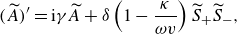(5.8) \begin{align} (\widetilde {A})^{\prime}= \textrm {i}{\gamma } \widetilde {A}+\delta \left ({1-\frac {\kappa }{\omega v}}\right){\widetilde {S}_+ \widetilde {S}_-}, \end{align}

(5.9) \begin{align} (\widetilde {S}_{\pm })^{\prime} = -{\frac {\delta }{2} \,\left |1-\frac {\kappa }{\omega v}\right |} \widetilde {A} \widetilde {S}_{\mp }^*-\textrm {i}\lambda \left |1-\frac {\kappa }{\omega v}\right | \left (1-\frac {\kappa }{\omega v}\right)\left (\widetilde {S}_{\pm }^2\widetilde {S}_{\pm }^*-{ 2}|\widetilde {S}_{\mp }|^2\widetilde {S}_{\pm }\right)\,. \end{align}

Here, the derivative $^{\prime}$ refers to differentiation with respect to $\tilde {\xi }$ in the moving frame. We identify two subcases based on the sign of $(1-{\kappa }/{\omega v})$ . Subcase (ii-1): $(1-{\kappa }/{\omega v})\lt 0$ . This scenario represents a singularity that signifies an ‘explosive’ breakdown of the equations after a finite time. We remark that, as noted in Craik (1986), this does not contradict the conservation laws. Rather, the conserved quantities $|\widetilde {A}|^2 - 2 |\widetilde {S}_\pm |^2$ are no longer signdefinite: see (Craik 1986, Section 14.3). Due to this unphysical behaviour, we discard the analysis of these solutions for the remainder of this discussion – more on such solutions can be found in (Coppi, Rosenbluth & Sudan 1969).

Subcase (ii-2): $0\lt (1-{\kappa }/{\omega v})$ . This case is well behaved and aligns with the previous analyses presented in § 3. In fact, the rescaled system is analogous to the one studied in that section if we make the following transformations:

(5.10) \begin{align} S_\pm \to \frac {{S}_\pm }{\sqrt {1-{\kappa }/{\omega v}}}\,, \qquad \alpha \to \left (1-\frac {\kappa }{\omega v}\right) \alpha \,, \qquad T \to \frac {T - {X}/{v}}{1-{\kappa }/{\omega v}} \,, \end{align}

while $A$ and $\gamma$ remain unchanged. Corresponding to the change (5.10), due to their dependence on $\alpha$ the constants $\delta$ and $\lambda$ are replaced by $ (1-{\kappa }/{\omega v}) \delta$ and $ (1-{\kappa }/{\omega v})^2 \lambda$ , respectively.

In summary, assuming $\kappa /\omega \gt 0$ , we conclude that a travelling-wave solution with velocity $v$ is stable (in the sense that the amplitudes remain bounded) only if ${\kappa /\omega }\leqslant v$ , namely when $v\in (-\infty, 0)\cup [\kappa /\omega, \infty)$ . This unusual condition on the velocity has a straightforward interpretation. In the stable case, the travelling wave is governed by the solution to equations (5.8)–(5.9), which are typically periodic, with period $\tau \gt 0$ (depending on the initial amplitudes and the velocity $v$ through the mapping in (5.10)). Thus, the travelling wave, being a function of $T-X/v$ , is periodic not only in time but also in space, with wavelength $\lambda = v\tau$ and wavenumber $k =1/{\lambda }$ . The wavenumber $k$ can take either sign: $k\gt 0$ corresponds to a wave travelling from left to right, while $k \lt 0$ corresponds to a wave travelling from right to left. Therefore, the condition for stability becomes $-\infty \lt k \leqslant {\omega }/{\kappa \tau },$ which covers a continuous range of wavenumbers, including all perturbations propagating from right to left as well as an infrared (i.e. ‘long-wave’) range of perturbations propagating from left to right.

5.2. Spatio-temporal resonant interactions

In the moving frame of reference with velocity $v$ , the equations for the spatio-temporal evolution of interacting acoustic–gravity waves, (5.8)–(5.9), are formally similar to their spatially independent counterparts, (3.1)–(3.2). Consequently, the same approach employed in § 3 can be applied to analyse this system.

By expressing each complex amplitude in exponential form, separating real and imaginary parts and deriving an equation for the dynamical phase, we find

(5.11) \begin{align} \theta ^{\prime} = -\gamma + \Lambda \left ( s_+^2 + s_-^2 \right) - \left [ \Gamma \left ( \frac {a s_-}{s_+} + \frac {a s_+}{s_-} \right) + \frac {\Delta s_+ s_-}{a} \right] \sin \theta, \end{align}

where

(5.12) \begin{align} \Delta \equiv \delta \left ( 1- \frac {\kappa }{\omega v} \right), \quad \Gamma \equiv - \frac {\delta }{2} \left |1- \frac {\kappa }{\omega v}\right |, \quad \Lambda \equiv \lambda \left \vert 1-\frac {\kappa }{\omega v} \right \vert \left ( 1- \frac {\kappa }{\omega v} \right). \end{align}

We focus on the case $v\in (-\infty,0) \cup ({\kappa }/{\omega },\infty),$ where the system simplifies to

(5.13) \begin{align} a^{\prime} = \Delta s_+ s_- \cos \theta; \qquad s_\pm ^{\prime} = -\frac {\Delta }{2} a s_\mp \cos \theta; \end{align}

(5.14) \begin{align} \theta ^{\prime} = -\gamma + \Lambda \left ( s_+^2 + s_-^2 \right) + \Delta \left [ \frac {a^2 s_-^2 + a^2 s_+^2 - 2s_+^2 s_-^2}{2 a s_+ s_-} \right] \sin \theta. \end{align}

By employing the transformation (3.9), we rewrite this as a planar system with the Hamiltonian

(5.15) \begin{align} H = \varDelta \sqrt {(\eta - W)(K^2 - \eta ^2)} \sin \theta - \eta \left ( \gamma - \frac {\Lambda \eta }{2} \right). \end{align}

Note that, as the velocity $v$ is increased to zero, the Hamiltonian $H$ becomes positive everywhere. Conversely, as $v$ is decreased to $\kappa /\omega$ , the Hamiltonian becomes negative everywhere. In the limit $|v|\rightarrow \infty$ , the Hamiltonian reduces to the form described in § 3, corresponding to the case without spatial dependency (see (5.11)).

In the case of spatial dependency and a moving frame of reference, $v$ becomes an additional independent variable influencing the system’s dynamics. Figure 5 illustrates how variations in $v$ alter the wave-packet acoustic–gravity interaction, resulting in distinct dynamical behaviours. In all panels of figure 5 we fix $\gamma = 0.36,$ and select $K=0, \, W=2$ , consistent with the parameters used in figure 1. For large positive and negative values of $v$ , the dynamics converges to that seen in panel (a) of figure 1. This is exemplified in panel (f) of figure 5, where a numerical value of $v=500$ was used to approximate the asymptotic ( $v=\infty$ ) values of the Hamiltonian to within three significant figures. As the velocity approaches the exclusion zone $[0,\kappa /\omega),$ the interaction diminishes and eventually disappears, as demonstrated in panels (a)–(c) of figure 5. This behaviour is consistent with the simple solution found in (5.4). For $v\gt \kappa /\omega$ , the bifurcation process is essentially the same as that observed in figure 1 when the detuning parameter $\gamma \gg 1$ is decreased. The corresponding dynamics, discussed in § 3, is similarly recovered in this case, including the case of asymptotic energy conversion, which is recovered at values of $v$ that solve $\gamma =\Lambda W/2$ as shown in figure 5 (e).

Figure 5. Phase portraits for the spatio-temporal system with varying speed $v.$ Parameter choices are as in panel (a) of figure 1, with $v=-0.5$ (a), $v=-0.25$ (b), $v=\kappa /\omega \approx 0.537$ (c), $v=0.805$ (d), $v\approx 1.18$ (e) and $v=\infty$ (f). Each curve is a level line of the Hamiltonian, so that trajectories of the system in $(\eta,\theta)$ remain confined to these level lines; fixed points are denoted by circles ( $\bigcirc$ ), and separatrices connecting these fixed points are denoted by dashed, black curves. Note that panel (f) of this figure is identical to panel (a) of figure 1.

6. Discussion and concluding remarks

The analysis presented in this study highlights the intricate dynamics of resonant triads involving acoustic–gravity wave interactions, with particular emphasis on spatial and temporal dependencies of wave amplitude. Considering the amplitude evolution equations derived by Kadri & Akylas (2016), we employed a dynamical systems approach to investigate bifurcation structures, steady-state resonances and optimal energy transfer conditions. This investigation provides new insights into the interplay between acoustic and surface modes in compressible fluids, enriching the broader understanding of nonlinear wave interactions.

Our results confirm that the triad phase or dynamical phase (Bustamante & Kartashova 2009; Harris et al. 2012) – a kind of phase difference between interacting modes – plays a pivotal role in energy exchange. When the dynamical phase aligns optimally along the separatrices, complete energy transfer between surface and acoustic modes becomes achievable. For the symmetric case ( $K = 0$ ), the bifurcation analysis revealed solutions corresponding to total energy conversion from surface to acoustic modes. For the asymmetric case ( $K \neq 0$ ), although complete conversion is unattainable, substantial energy redistribution still occurs, governed by the conserved quantities $W$ and $K$ . These findings complement earlier observations of the energy exchange dynamics in acoustic–gravity systems (Kadri & Akylas 2016).

The HAM methodology is the state-of-the-art in identifying steady-state resonances, having been employed successfully in a variety of physical configurations ranging from surface water waves (Liao, Xu & Stiassnie 2016) to Bragg scattering (Xu et al. 2012, 2023). Nevertheless, the simple and transparent methodology adopted herein makes the identification of steady-state acoustic–gravity wave triads simple for a variety of parameter values, and may provide impetus for further investigation using more highly nonlinear approaches. Moreover, putting these steady states into a natural context as fixed points of a dynamical system more clearly illustrates their role in the dynamics of energy exchange between surface and acoustic modes, as well as other resonant interaction processes (Andrade & Stuhlmeier 2023b ).

Our model equations for acoustic–gravity wave interaction take into account the leading terms up to and including cubic nonlinearities. It is therefore encouraging to see that the weakly nonlinear analysis captures features of the acoustic–gravity wave problem in the fully nonlinear compressible equations, as explored using HAM by Yang et al. (2018); Yang & Yang (2024). While an exact, Gerstner-like acoustic–gravity wave solution was found by Godin (2015), the wider landscape of fully nonlinear progressive acoustic–gravity wave solutions remains to be explored, both analytically and numerically.

The incorporation of spatial dependency into the triad dynamics introduces new and richer behaviours, dependent on the wave velocity $v$ . While the bifurcation structure observed in the spatially independent case remains robust, the inclusion of the spatial dynamics introduces modulations in periodic solutions and stability conditions, thereby expanding the applicability of this framework. This aligns with the broader scope of acoustic–gravity wave studies, including the generation of microseisms (Longuet-Higgins 1950; Kibblewhite & Ewans 1985), and the amplification of tsunami amplitude as in the case of the 2022 Hunga-Tonga Hunga Ha’apai eruption (Omira et al. 2022). It is worth noting that, although the Tonga case primarily involves the propagation of acoustic–gravity waves in the atmosphere, their coupling with water waves (the generated meteotsunami) occurs at the interface (water surface), which, in principle, follows the same mechanism as described in Kadri & Akylas (2016), with only minor modifications. Nevertheless, further research into the two-layer problem would be necessary to achieve a more rigorous and specific result. Moreover, the complete energy conversion observed in this study could have potential applications in the development of new energy-harnessing technologies. The triad resonance mechanism may be exploited to enhance energy capture and amplification in such systems.

Future research directions include the investigation of the nonlinear interaction of two acoustic modes interacting with a single gravity wave (Kadri 2016, 2017; Zuccoli & Kadri 2025), a context in which steady-state resonances have been recently identified using the HAM (Yang & Yang 2024). Further extension of the model could account for additional physical effects such as seabed elasticity (Eyov et al. 2013; Williams & Kadri 2023), stratification (Michele & Renzi 2020), background currents and higher-order nonlinearities. The coupling between broad-banded ocean wave spectra and multiple compressibility modes, and the attendant role of dynamical phase in stochastic evolution equations (Andrade & Stuhlmeier 2023a ), also remain important challenges. Finally, we expect that laboratory experiments, supported by numerical simulations, could be carried out to validate and refine the analytical predictions presented here, particularly in scenarios where spatially modulated triads introduce complex dynamical behaviours. In such cases, triad resonance involving higher acoustic modes may become more accessible, especially when flume depths are insufficient to support the leading mode efficiently. Experimental investigations in this direction are currently ongoing.