


1. Introduction
The interaction between acoustic waves and fluids spawns an oscillatory fluid flow concomitant with the wave’s propagation and in addition to that, a mean flow known as acoustic streaming emerges over time. The oscillatory flow delineates the fast time scale, and for monochromatic acoustic wave propagation in a fluid, the temporal scale of this oscillatory flow is well described by the time period of the acoustic wave. Conversely, the mean fluid flow characterises the slow time scale associated with the system’s hydrodynamics. The attenuation of the acoustic wave in the fluid results in Reynolds stress divergence, which acts as a body force, instigating the mean flow (Lighthill Reference Lighthill1978). Based on the nature of the attenuation, acoustic streaming can be broadly categorised into two categories: boundary-layer-driven streaming and Eckart streaming. In boundary-layer-driven streaming, Schlichting streaming (Schlichting Reference Schlichting1932) is engendered adjacent to the fluid/solid boundary, via vibrations from the solid, whereas Rayleigh streaming (Rayleigh Reference Rayleigh1885) is instigated by the propagation of acoustic waves through the bulk fluid medium. Schlichting or Rayleigh streaming is predominant in small fluid chambers whose dimensions are of the order of a few acoustic wavelengths. In contrast, in larger fluid geometries, the attenuation results from viscous dissipation within the fluid bulk, culminating in the generation of Eckart streaming (Eckart Reference Eckart1948). This phenomenon of acoustic streaming is harnessed in a myriad of biochemical and medical science applications, including particle separation and manipulation (Shi et al. Reference Shi, Ahmed, Mao, Lin, Lawit and Huang2009; Wang & Zhe Reference Wang and Zhe2011; Augustsson et al. Reference Augustsson, Magnusson, Nordin, Lilja and Laurell2012; Lei, Glynne-Jones & Hill Reference Lei, Glynne-Jones and Hill2013; Li et al. Reference Li, Lv, Zhang, Saeed and Deng2016), cell trapping (Ahmed et al. Reference Ahmed, Ozcelik, Bojanala, Nama, Upadhyay, Chen, Hanna-Rose and Huang2016; Guo et al. Reference Guo2016; Ozcelik et al. Reference Ozcelik, Rufo, Guo, Gu, Li, Lata and Huang2018), cell lysis (Wu et al. Reference Wu2017), biosensing (Liu, Li & Bhethanabotla Reference Liu, Li and Bhethanabotla2018; Huang et al. Reference Huang, Sun, Hu, Han and Lei2021) and the removal of non-specific binding (Cular, Sankaranarayanan & Bhethanabotla Reference Cular, Sankaranarayanan and Bhethanabotla2008; Sankaranarayanan, Singh & Bhethanabotla Reference Sankaranarayanan, Singh and Bhethanabotla2010; Hsu et al. Reference Hsu, Feng, Cho and Chau2013), among others. The attenuation of acoustic waves and the generation of coherent acoustic streaming patterns have, hitherto, remained poorly understood phenomena, prompting significant research efforts to elucidate these complex interactions. Eckart highlighted that the hydrodynamic body force driving acoustic streaming is linearly proportional to both shear and bulk viscosities. Lighthill further elucidated that the attenuation of acoustic energy flux generates Reynolds stress divergence (Lighthill Reference Lighthill1978), which serves as the driving force for acoustic streaming. In contrast to Shiokawa, Matsui & Moriizumi (Reference Shiokawa, Matsui and Moriizumi1989), who proposed that acoustic wave attenuation occurs solely within the boundary layer, thereby driving the fluid motion in the inviscid bulk, Vanneste & Bühler (Reference Vanneste and Bühler2011) illustrated that streaming within the bulk predominates over effects within the boundary layer.
However, the interaction between fluids and acoustic waves is further complicated by acoustothermal effect. Kondoh et al. (Reference Kondoh, Shimizu, Matsui and Shiokawa2005) were pioneers in demonstrating that surface acoustic waves (SAW) can induce heating in a water film, revealing that acoustothermal temperature rise is contingent on the applied SAW voltages. Subsequent studies have delved into the effects of liquid viscosity, duty cycle, fluid volume and intermittent SAW actuation, among others, on this heating phenomenon (Kondoh et al. Reference Kondoh, Shimizu, Matsui, Sugimoto and Shiokawa2009; Shilton et al. Reference Shilton2015; Zhang et al. Reference Zhang, Zhang, Fu and Zha2015; Rahimzadeh et al. Reference Rahimzadeh, Rutsch, Kupnik and Klitzing2021; Wang et al. Reference Wang2021). This acoustothermal effect is of paramount importance, as it both constrains and broadens its applications across diverse fields. For instance, this heating effect can be leveraged in sessile droplet-based microfluidic systems to elevate temperatures for conducting specific polymerase chain reactions (Kulkarni et al. Reference Kulkarni, Friend, Yeo and Perlmutter2009), or in diagnostic technologies (Reboud et al. Reference Reboud, Bourquin, Wilson, Pall, Jiwaji, Pitt, Graham, Waters and Cooper2012). To ascertain liquid droplet temperatures adequate for these applications, Roux-Marchand et al. (Reference Roux-Marchand, Beyssen, Sarry and Elmazria2013) investigated the temperature uniformity during the SAW-induced heating and concluded that lower SAW frequencies yield higher uniformity within the droplet. These examples highlight widening applications of the acoustothermal effect, albeit that it causes hindrances in certain contexts. For instance, in biosensing applications, SAW has demonstrated efficacy in removing non-specific bindings, but higher SAW power can lead to substantial temperature increases, potentially damaging bio-analytes. Thus, a comprehensive understanding of these phenomena from both theoretical and experimental perspectives is crucial.
All of the aforementioned studies on acoustothermal effect are predominantly experimental, with theoretical investigations being relatively scarce. Moreover, research efforts have primarily focused on understanding the acoustic streaming phenomena, rather that diving into the specifics of the associated heat generation. Li et al. (Reference Li, Wu, Jia and Yang2021) conducted both experimental and theoretical investigations to elucidate the temperature non-uniformity in droplets induced by the acoustothermal effect. They meticulously measured temperatures in 1, 4 and 6 ![]() droplets composed of pure water and water–glycerol mixtures. Their theoretical work involved comprehensive modelling of the piezoelectric solid, interdigital transducers (IDTs) and water droplets, aiming to provide an extensive understanding of the acoustothermal effect. However, their study is constrained by the acoustothermal heat source calculations, which were carried out using a two-dimensional computational domain, thereby lacking the three-dimensional perspective necessary for precise and accurate computation. More recently, Joergensen & Bruus (Reference Joergensen and Bruus2023) developed a rigorous thermoviscous acoustic model, demonstrating that the acoustothermal effect arises exclusively from viscous dissipation within the boundary layer, with no significant contribution from the fluid bulk. Their results revealed a maximum temperature increase of only 1.5
droplets composed of pure water and water–glycerol mixtures. Their theoretical work involved comprehensive modelling of the piezoelectric solid, interdigital transducers (IDTs) and water droplets, aiming to provide an extensive understanding of the acoustothermal effect. However, their study is constrained by the acoustothermal heat source calculations, which were carried out using a two-dimensional computational domain, thereby lacking the three-dimensional perspective necessary for precise and accurate computation. More recently, Joergensen & Bruus (Reference Joergensen and Bruus2023) developed a rigorous thermoviscous acoustic model, demonstrating that the acoustothermal effect arises exclusively from viscous dissipation within the boundary layer, with no significant contribution from the fluid bulk. Their results revealed a maximum temperature increase of only 1.5 $^{\circ }$
C in a rectangular microchannel, with dimensions comparable to the acoustic wavelength, albeit that the acoustic energy density was extremely high (
$^{\circ }$
C in a rectangular microchannel, with dimensions comparable to the acoustic wavelength, albeit that the acoustic energy density was extremely high ( ${\sim}5300 \, \mathrm{J\,m^-{^3}}$
). As previously mentioned, the ultrasonic shearing effect within the boundary layer and the fluid bulk attenuation of the acoustic waves generate Rayleigh and Eckart streaming, respectively. Similarly, it is crucial to comprehend the fundamental source of acoustothermal heat beyond the confines of the boundary layer effect. Furthermore, acoustothermal heating is predominantly observed in systems where the fluid volume is large relative to the acoustic wavelength and Eckart streaming dominates over Rayleigh streaming. Consequently, there exists a gap in our understanding of the overarching mechanism of the acoustothermal effect, irrespective of the specific streaming mechanism. This knowledge gap in acoustofluidics motivates our study, aiming to delve deeper into the underlying mechanisms of acoustothermal heating and to offer a closed-form quantification of the heat source.
${\sim}5300 \, \mathrm{J\,m^-{^3}}$
). As previously mentioned, the ultrasonic shearing effect within the boundary layer and the fluid bulk attenuation of the acoustic waves generate Rayleigh and Eckart streaming, respectively. Similarly, it is crucial to comprehend the fundamental source of acoustothermal heat beyond the confines of the boundary layer effect. Furthermore, acoustothermal heating is predominantly observed in systems where the fluid volume is large relative to the acoustic wavelength and Eckart streaming dominates over Rayleigh streaming. Consequently, there exists a gap in our understanding of the overarching mechanism of the acoustothermal effect, irrespective of the specific streaming mechanism. This knowledge gap in acoustofluidics motivates our study, aiming to delve deeper into the underlying mechanisms of acoustothermal heating and to offer a closed-form quantification of the heat source.
In this work, we investigate the acoustothermal temperature rise in a sessile droplet driven by SAW fields, both theoretically and experimentally. We highlight the inadequacy of the regular perturbation technique and, consequently, develop a rigorous and comprehensive theoretical model based on multiple time scales. This model captures the essential physics and elucidates the critical parameters governing acoustothermal heat generation. Our principal findings are as follows: (i) the propagation of acoustic power within the fluid is exclusively characterised by the acoustic Poynting vector, analogous to the behaviour of electromagnetic waves. (ii) The acoustic power flows coherently along the direction of the acoustic wave propagation. (iii) While the acoustothermal heat generation rate is determined by the negative divergence of the Poynting vector, entailing both the rate of increase in acoustic energy density and the power absorbed through viscous damping, the time-averaged heat generation rate is solely defined by the time-averaged power loss spawned by viscous damping. While in this work we employ counterpropagating SAWs, emanating from IDTs positioned in opposite directions, and characterise the temperature rise of a sessile droplet placed on the delay path, our theoretical framework generalises immediately to any kind of acoustofluidic system. The fundamental insights into the acoustothermal effect are of paramount relevance to the broader community working in microfluidics and acoustics, given the bidirectional coupling with thermoacoustic streaming, which significantly alters the flow field or vice versa. The findings of the present study will not only bridge the knowledge gap in acoustofluidics but also pave the way for designing advanced and complex acoustofluidic systems.
2. Experimental
2.1. Device design
The acoustothermal experiments were performed on a SAW device where the standing SAW was generated via the superposition of two waves of equal wavelength and amplitude travelling towards each other with a phase difference that is an integer multiple of $\pi$
. The SAW device employed in this study comprises 20 pairs of IDTs etched onto both sides of a 128
$\pi$
. The SAW device employed in this study comprises 20 pairs of IDTs etched onto both sides of a 128 $^\circ$
Y-cut X-propagating lithium niobate (LiNbO
$^\circ$
Y-cut X-propagating lithium niobate (LiNbO $_3$
) substrate. The device was fabricated using a conventional SAW fabrication process, which involves coating the lithium niobate substrate with photoresist, followed by ultraviolet exposure, mask lithography, aluminium deposition and, finally, lift-off. Aluminium was deposited to form a patterned layer with a thickness of 100 nm. When both pairs of IDTs are excited with an AC signal, standing SAWs are generated on the top surface of the lithium niobate. To generate a SAW with wavelength
$_3$
) substrate. The device was fabricated using a conventional SAW fabrication process, which involves coating the lithium niobate substrate with photoresist, followed by ultraviolet exposure, mask lithography, aluminium deposition and, finally, lift-off. Aluminium was deposited to form a patterned layer with a thickness of 100 nm. When both pairs of IDTs are excited with an AC signal, standing SAWs are generated on the top surface of the lithium niobate. To generate a SAW with wavelength $\lambda = 120 \, \unicode{x03BC}\rm m$
, the spacing between two adjacent IDTs and the IDT width were both set to
$\lambda = 120 \, \unicode{x03BC}\rm m$
, the spacing between two adjacent IDTs and the IDT width were both set to $\lambda /4 = 30 \, \unicode{x03BC}\rm m$
. The actuation frequency of the SAW device was determined to be 32.016 MHz, corresponding to the minimum insertion loss (see § S1 in the Supplementary Material), and this frequency was used as the driving frequency for all experiments.
$\lambda /4 = 30 \, \unicode{x03BC}\rm m$
. The actuation frequency of the SAW device was determined to be 32.016 MHz, corresponding to the minimum insertion loss (see § S1 in the Supplementary Material), and this frequency was used as the driving frequency for all experiments.
2.2. Experimental set-up and data acquisition
The experimental set-up is illustrated in figure 1(a), where a sinusoidal signal was generated using a signal generator (Rohde & Schwarz, model SMA100A). Subsequently, the signal was amplified by a power amplifier (Mini-Circuits, model TIA-1000-1R8) and split to connect to both sides of the IDTs of the SAW device via a signal splitter. Ultrapure water droplets of 2 or $5 \, \unicode{x03BC}$
l were placed on the delay path of the SAW device and the average droplet contact angle was estimated to be
$5 \, \unicode{x03BC}$
l were placed on the delay path of the SAW device and the average droplet contact angle was estimated to be $ \phi _c \sim 100.6^\circ$
, based on three independent measurements (see § S2 in the Supplementary Material). To monitor droplet temperature over time, an infrared thermal camera (FLIR, model-T62101) was positioned perpendicularly above the sessile droplet using a camera stand, thereby minimising errors associated with distortions caused by droplet curvature. The thermal camera has a specified accuracy of
$ \phi _c \sim 100.6^\circ$
, based on three independent measurements (see § S2 in the Supplementary Material). To monitor droplet temperature over time, an infrared thermal camera (FLIR, model-T62101) was positioned perpendicularly above the sessile droplet using a camera stand, thereby minimising errors associated with distortions caused by droplet curvature. The thermal camera has a specified accuracy of $\pm$
2 °C or
$\pm$
2 °C or $\pm$
2 % of the reading (whichever is greater), with a temperature sensitivity of
$\pm$
2 % of the reading (whichever is greater), with a temperature sensitivity of ${\lt } 0.02$
°C, a spectral range of 7.5–14
${\lt } 0.02$
°C, a spectral range of 7.5–14 $\unicode{x03BC}\rm m$
and a resolution of 320
$\unicode{x03BC}\rm m$
and a resolution of 320 $\times$
240 pixels. To enhance measurement accuracy, we applied emissivity corrections calibrated to the object’s emissivity and maintained consistent droplet geometry to mitigate shape variations. Initially, the thermal camera was switched on to record, allowing 15 s to stabilise and reach a static temperature profile in absence of any SAW signal. After this initial period, the SAW signal was applied, marking the commencement of the experiment. In each experiment, the droplet was exposed to SAW for 90 s to attain steady-state temperature and then the SAW was switched off. After the SAW was off, the droplet temperature was recorded for another 90 s to allow the droplet to reach to ambient temperature. The choice of 90 s exposure time has been made to ensure that steady-state temperature is achieved. These heating experiments were conducted both in the presence and absence of the droplet, where experiments in the absence of a water droplet were carried out to explicitly quantify the heating of the lithium niobate substrate from non-acoustothermal effects such as Joule heating in the IDTs or heat due to dielectric loss. The thermal camera used in these experiments records at 30 frames per second, and the captured images were extracted and analysed using MATLAB’s image processing tools.
$\times$
240 pixels. To enhance measurement accuracy, we applied emissivity corrections calibrated to the object’s emissivity and maintained consistent droplet geometry to mitigate shape variations. Initially, the thermal camera was switched on to record, allowing 15 s to stabilise and reach a static temperature profile in absence of any SAW signal. After this initial period, the SAW signal was applied, marking the commencement of the experiment. In each experiment, the droplet was exposed to SAW for 90 s to attain steady-state temperature and then the SAW was switched off. After the SAW was off, the droplet temperature was recorded for another 90 s to allow the droplet to reach to ambient temperature. The choice of 90 s exposure time has been made to ensure that steady-state temperature is achieved. These heating experiments were conducted both in the presence and absence of the droplet, where experiments in the absence of a water droplet were carried out to explicitly quantify the heating of the lithium niobate substrate from non-acoustothermal effects such as Joule heating in the IDTs or heat due to dielectric loss. The thermal camera used in these experiments records at 30 frames per second, and the captured images were extracted and analysed using MATLAB’s image processing tools.

Figure 1. Acoustothermal effect in sessile droplets actuated by standing SAWs. (a) Schematic of the experimental set-up, wherein a standing SAW is generated via a signal generator, followed by amplification through a power amplifier and splitting by an Radio Frequency splitter. A thermal camera is employed to capture the evolution of the droplet’s temperature. (b) Timestamps of the temperature of a $2\,\unicode{x03BC}$
l sessile water droplet actuated by a
$2\,\unicode{x03BC}$
l sessile water droplet actuated by a $32.016 \, \text{MHz}$
standing SAW, captured by a thermal camera at 0, 2, 4, 6, 10 and 20 s, where
$32.016 \, \text{MHz}$
standing SAW, captured by a thermal camera at 0, 2, 4, 6, 10 and 20 s, where $\tau = 0$
marks the initiation of the standing SAW actuation. (c) The associated dynamics of the droplet temperature where
$\tau = 0$
marks the initiation of the standing SAW actuation. (c) The associated dynamics of the droplet temperature where $\tau = 90 \, \text{s}$
marks when the SAW actuation is stopped.
$\tau = 90 \, \text{s}$
marks when the SAW actuation is stopped.
3. Mathematical formulations
3.1. System description
The standing SAW-actuated droplet system, illustrated in figure 1(a), consists of a 128° Y-cut, X-propagating lithium niobate (LiNbO $_3$
) substrate patterned with IDTs and a sessile droplet positioned along the delay path. The generation of standing SAWs requires the excitation of IDTs with an AC signal at specific frequencies, creating counter-propagating waves on the piezoelectric substrate. A comprehensive and rigorous modelling of the physical system requires consideration of electrostatic, elastic and hydrodynamic interactions, which pose significant computational challenges, especially for three-dimensional (3-D) simulations. Quintero & Simonetti (Reference Quintero and Simonetti2013) conducted the only available study on 3-D simulations of sessile droplets involving solid–fluid coupling. They modelled a small droplet with a diameter of approximately
$_3$
) substrate patterned with IDTs and a sessile droplet positioned along the delay path. The generation of standing SAWs requires the excitation of IDTs with an AC signal at specific frequencies, creating counter-propagating waves on the piezoelectric substrate. A comprehensive and rigorous modelling of the physical system requires consideration of electrostatic, elastic and hydrodynamic interactions, which pose significant computational challenges, especially for three-dimensional (3-D) simulations. Quintero & Simonetti (Reference Quintero and Simonetti2013) conducted the only available study on 3-D simulations of sessile droplets involving solid–fluid coupling. They modelled a small droplet with a diameter of approximately $2\lambda$
, and instead of incorporating the complexities of piezoelectric coupling with electrostatic and elastic interactions, they modelled an ideal elastic solid generating SAWs. Additionally, they employed perfectly matched layers to suppress extraneous reflections and reduce the computational domain size. Even with this simplified system, they faced considerable challenges in accurately calculating acoustic fields at a relatively low frequency of 2.25 MHz. Skov et al. (Reference Skov, Sehgal, Kirby and Bruus2019) studied a 3-D SAW-actuated microchannel, noting the high memory demands of a fully coupled solid–fluid model. Despite downscaling, their 3-D simulation still required 80 nodes and 14 hours on a high-performance computing cluster. These highlight the profound complexities associated with modelling 3-D acoustofluidic systems, particularly for large-scale systems (
$2\lambda$
, and instead of incorporating the complexities of piezoelectric coupling with electrostatic and elastic interactions, they modelled an ideal elastic solid generating SAWs. Additionally, they employed perfectly matched layers to suppress extraneous reflections and reduce the computational domain size. Even with this simplified system, they faced considerable challenges in accurately calculating acoustic fields at a relatively low frequency of 2.25 MHz. Skov et al. (Reference Skov, Sehgal, Kirby and Bruus2019) studied a 3-D SAW-actuated microchannel, noting the high memory demands of a fully coupled solid–fluid model. Despite downscaling, their 3-D simulation still required 80 nodes and 14 hours on a high-performance computing cluster. These highlight the profound complexities associated with modelling 3-D acoustofluidic systems, particularly for large-scale systems ( ${\gg}\lambda$
) and at higher operating frequencies.
${\gg}\lambda$
) and at higher operating frequencies.
To address the challenges of modelling SAW-driven systems, a viable approach could involve using a two-dimensional (2-D) model with coupled piezoelectric–fluid interactions. Fakhfouri et al. (Reference Fakhfouri, Devendran, Albrecht, Collins, Winkler, Schmidt and Neild2018) demonstrated this by simulating a simplified 2-D fully coupled model of a lithium niobate substrate and a fluid-filled polydimethylsiloxane microchannel to predict acoustic streaming. Their numerical predictions aligned closely with experimental results. It is important to note here that, while 2-D models have shown efficacy in numerous acoustofluidic applications, they are not suited for accurately representing SAW-driven sessile water droplet systems as they fail to precisely calculate the acoustic fields within the sessile droplet, resulting in inaccuracies in heat source estimations (Li et al. Reference Li, Wu, Jia and Yang2021). This underscores the necessity of adopting a 3-D model for accurate analysis of SAW-driven sessile water droplets. Given the prohibitive complexity of fully modelling 3-D piezoelectric–fluid coupled systems, a pragmatic alternative involves using SAW displacement fields at the droplet base. These displacement fields decay exponentially with depth into the substrate, effectively concentrating the majority of wave energy at the surface. The wave motions in the $x$
- and
$x$
- and $z$
-directions exhibit a phase shift of 90
$z$
-directions exhibit a phase shift of 90 $^{\circ }$
, generating elliptical displacement patterns. Gantner et al. (Reference Gantner, Hoppe, Köster, Siebert and Wixforth2007) conducted a comprehensive numerical analysis of SAWs in piezoelectric substrates, offering critical insights into the behaviour and properties of these displacement fields. This approach effectively balances computational feasibility with the need for accuracy in modelling complex SAW-driven systems. The use of SAW displacement fields as a substitute for fully coupled piezoelectric–fluid models is further demonstrated in studies by Devendran et al. (Reference Devendran, Albrecht, Brenker, Alan and Neild2016), Tan & Yeo (Reference Tan and Yeo2018) and Barnkob et al. (Reference Barnkob, Nama, Ren, Huang, Costanzo and Kähler2018), whose 2-D numerical predictions matched experimental results with high precision. Moreover, their findings qualitatively align with Fakhfouri et al.’s (Reference Fakhfouri, Devendran, Albrecht, Collins, Winkler, Schmidt and Neild2018) results, where a fully coupled 2-D model was employed.
$^{\circ }$
, generating elliptical displacement patterns. Gantner et al. (Reference Gantner, Hoppe, Köster, Siebert and Wixforth2007) conducted a comprehensive numerical analysis of SAWs in piezoelectric substrates, offering critical insights into the behaviour and properties of these displacement fields. This approach effectively balances computational feasibility with the need for accuracy in modelling complex SAW-driven systems. The use of SAW displacement fields as a substitute for fully coupled piezoelectric–fluid models is further demonstrated in studies by Devendran et al. (Reference Devendran, Albrecht, Brenker, Alan and Neild2016), Tan & Yeo (Reference Tan and Yeo2018) and Barnkob et al. (Reference Barnkob, Nama, Ren, Huang, Costanzo and Kähler2018), whose 2-D numerical predictions matched experimental results with high precision. Moreover, their findings qualitatively align with Fakhfouri et al.’s (Reference Fakhfouri, Devendran, Albrecht, Collins, Winkler, Schmidt and Neild2018) results, where a fully coupled 2-D model was employed.
Riaud et al. (Reference Riaud, Baudoin, Bou Matar, Thomas and Brunet2017) investigated a system closely resembling the present study, focusing on acoustic streaming within sessile water–glycerol droplets driven by a travelling SAW. The work emphasised the computational complexity of such theoretical and numerical investigations, even with modern computational resources. Employing a 20 MHz SAW, they confined their modelling to the fluidic domain, deliberately eschewing the fully coupled piezoelectric–fluid theoretical framework and incorporating solely the vertical component of the SAW displacement field at the droplet’s base. Their numerical predictions aligned well with experiments, demonstrating the approach’s reliability. Nevertheless, their study highlighted the formidable computational challenges inherent in modelling these systems and revealed that the computational memory demands for acoustic field computations increase exponentially with higher SAW frequencies, underscoring the significant computational burden of such acoustofluidic systems.
Building on this understanding, in the present study we focus on developing a comprehensive theoretical formulation for the acoustothermal effect within the fluid only and this involves considering appropriate acoustic displacement fields at the fluid boundary to accurately characterise the fluid–acoustic interaction. We denote fluid density, pressure, energy, temperature and thermal conductivity as $ \rho$
,
$ \rho$
, $ p$
,
$ p$
, $ E$
,
$ E$
, $ T$
and
$ T$
and $ k_{th}$
, respectively. The conservations of mass, momentum and energy are given by
$ k_{th}$
, respectively. The conservations of mass, momentum and energy are given by
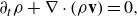 \begin{equation} \partial _t \rho + \nabla \cdot (\rho \mathbf{v}) = 0,\end{equation}
 \begin{equation} \rho \left [ \partial _t \mathbf{v} + (\mathbf{v} \cdot \nabla) \mathbf{v} \right] = -\nabla p + \mu \nabla ^2 \mathbf{v} + \mu \beta \nabla (\nabla \cdot \mathbf{v}),\end{equation}
 \begin{equation} \partial _t \left ( \rho E + \frac {1}{2} \rho \textit{v}^2 \right) = \nabla \cdot \left [ \mathbf{v} \cdot \boldsymbol{\sigma } - p \mathbf{v} + k_{{th}} \nabla T - \rho \left ( E + \frac {1}{2} \textit{v}^2 \right) \mathbf{v} \right], \end{equation}
where $\beta = {1}/{3} + {\mu _b}/{\mu }$
. The velocity field is given by
$\beta = {1}/{3} + {\mu _b}/{\mu }$
. The velocity field is given by $\mathbf{v} = v_x \mathbf{e}_x + v_y \mathbf{e}_y + v_z \mathbf{e}_z$
, where
$\mathbf{v} = v_x \mathbf{e}_x + v_y \mathbf{e}_y + v_z \mathbf{e}_z$
, where $ \mathbf{e}_x$
,
$ \mathbf{e}_x$
, $ \mathbf{e}_y$
and
$ \mathbf{e}_y$
and $ \mathbf{e}_z$
are unit vectors along the
$ \mathbf{e}_z$
are unit vectors along the $ x$
,
$ x$
, $ y$
and
$ y$
and $ z$
directions, respectively. In these equations,
$ z$
directions, respectively. In these equations, $ \textit{v}^2 = |\mathbf{v}|^2$
,
$ \textit{v}^2 = |\mathbf{v}|^2$
, $\boldsymbol{\sigma } = \mu [ \nabla \mathbf{v} + (\nabla \mathbf{v})^T] + (\mu _b - ({2}/{3}) \mu) (\nabla \cdot \mathbf{v}) \mathbf{I}$
is the stress tensor, superscript
$\boldsymbol{\sigma } = \mu [ \nabla \mathbf{v} + (\nabla \mathbf{v})^T] + (\mu _b - ({2}/{3}) \mu) (\nabla \cdot \mathbf{v}) \mathbf{I}$
is the stress tensor, superscript $ T$
indicates the transpose of a matrix, I is the identity matrix, while
$ T$
indicates the transpose of a matrix, I is the identity matrix, while $ \mu$
and
$ \mu$
and $ \mu _b$
denote shear and bulk viscosity, respectively.
$ \mu _b$
denote shear and bulk viscosity, respectively.
We have chosen an appropriate coordinate system, as shown in figure 1(a), and the droplet is assumed to be positioned on the $ z = 0$
plane with its base centred at the origin, resting at a contact angle
$ z = 0$
plane with its base centred at the origin, resting at a contact angle $ \phi _c$
with the substrate. The droplet base radius (
$ \phi _c$
with the substrate. The droplet base radius ( $ R_{{base}}$
) can be derived from the droplet volume (
$ R_{{base}}$
) can be derived from the droplet volume ( $ V_s$
) and the contact angle (
$ V_s$
) and the contact angle ( $ \phi _c$
) as
$ \phi _c$
) as $R_{{base}} = ( ({3V_s})/({\pi [ 2 - \cos \phi _c (3 - \cos ^2 \phi _c)]})^{1/3} \sin \phi _c$
, where
$R_{{base}} = ( ({3V_s})/({\pi [ 2 - \cos \phi _c (3 - \cos ^2 \phi _c)]})^{1/3} \sin \phi _c$
, where $ R_{{base}}$
is related to the droplet radius (
$ R_{{base}}$
is related to the droplet radius ( $ R$
) as
$ R$
) as $ R_{{base}} = R \sin \phi _c$
. The standing SAW interacts with the droplet through actuation at the bottom. Consequently, a no-slip boundary condition is enforced at the droplet base, prescribing the fluid particle displacement according to the standing SAW displacement field. Furthermore, our analysis is confined to the acoustothermal heating within the sessile droplet, with necessary adjustments made to account for the temperature rise within the piezoelectric substrate. Accordingly, the following conditions are applied:
$ R_{{base}} = R \sin \phi _c$
. The standing SAW interacts with the droplet through actuation at the bottom. Consequently, a no-slip boundary condition is enforced at the droplet base, prescribing the fluid particle displacement according to the standing SAW displacement field. Furthermore, our analysis is confined to the acoustothermal heating within the sessile droplet, with necessary adjustments made to account for the temperature rise within the piezoelectric substrate. Accordingly, the following conditions are applied:
 \begin{equation} \begin{aligned} \tilde {u} &= \xi u_0 \left [ e^{-i k_x x} e^{-\alpha _{{SAW}} (x - x_0)} + e^{i k_x x} e^{\alpha _{{SAW}} (x + x_0)} \right] e^{i \omega t} \mathbf{e}_x \\ &\quad + u_0 \left [ e^{-i \left ( k_x x - \frac {3\pi }{2} \right)} e^{-\alpha _{{SAW}} (x - x_0)} + e^{i \left ( k_x x + \frac {\pi }{2} \right)} e^{\alpha _{{SAW}} (x + x_0)} \right] e^{i \omega t} \mathbf{e}_z, \end{aligned} \end{equation}
 \begin{equation} T = T_b,\end{equation}
where $x_0 = \sqrt {R^2 - y^2}$
;
$x_0 = \sqrt {R^2 - y^2}$
; $ \omega$
and
$ \omega$
and $ k_x$
are the angular frequency and wave vector of the SAW, respectively, and
$ k_x$
are the angular frequency and wave vector of the SAW, respectively, and $ T_b$
is the droplet bottom temperature. The SAW attenuation coefficient is given by
$ T_b$
is the droplet bottom temperature. The SAW attenuation coefficient is given by $\alpha _{{SAW}} = ({\rho c_0})/({\rho _{{LN}} c_{{LN}} \lambda })$
, where
$\alpha _{{SAW}} = ({\rho c_0})/({\rho _{{LN}} c_{{LN}} \lambda })$
, where $ \rho _{{LN}}$
and
$ \rho _{{LN}}$
and $ c_{{LN}}$
are the density of lithium niobate and the sonic speed in lithium niobate, respectively,
$ c_{{LN}}$
are the density of lithium niobate and the sonic speed in lithium niobate, respectively, $ c_0$
is the sonic speed in the fluid and
$ c_0$
is the sonic speed in the fluid and $ \xi$
denotes the ratio of longitudinal to transverse wave amplitudes.
$ \xi$
denotes the ratio of longitudinal to transverse wave amplitudes.
At the free surface, convective heat loss and zero pressure conditions are prescribed
 \begin{equation} p = 0, \end{equation}
 \begin{equation} \mathbf{n} \cdot \left ( -k_{{th}} \nabla T \right) = h_{{amb}} \left ( T - T_0 \right), \end{equation}
where $\mathbf{n}$
is the unit vector along the surface normal,
$\mathbf{n}$
is the unit vector along the surface normal, $T_0$
is the ambient temperature and
$T_0$
is the ambient temperature and $h_{{amb}}$
is the convective heat transfer coefficient.
$h_{{amb}}$
is the convective heat transfer coefficient.
3.2. Separation of time scales
Based on the inherent dynamics, the flow and temperature fields of the acoustofluidic system can be characterised by two distinct time scales: (i) fast and (ii) slow time scales. The fast time scale is typically associated with the oscillation period of the acoustic waves and can be denoted as $t = \omega ^{-1}$
. The slow time scale (
$t = \omega ^{-1}$
. The slow time scale ( $\tau$
) pertains to the thermo-hydrodynamics of the system and is generally much larger than the fast time scales (
$\tau$
) pertains to the thermo-hydrodynamics of the system and is generally much larger than the fast time scales ( $\tau \gg t$
).
$\tau \gg t$
).
In the context of the slow time scale, we are interested in the mean flow and temperature fields, where the components of flow and temperature fields on the fast time scale serve as the driving forces in the slow thermo-hydrodynamics. Moreover, regular perturbation techniques cannot be applied since the thermo-hydrodynamic temperature rise often exceeds the acoustic temperature fields. Hence, we write any physical response associated with the acoustofluidic systems as the sum of mean ( $\bar {g}$
) and fast oscillatory (
$\bar {g}$
) and fast oscillatory ( $\tilde {g}$
) components
$\tilde {g}$
) components
 \begin{equation} g = \bar {g}(x, y, z, \tau) + \tilde {g}(x, y, z, t). \end{equation}
To obtain the mean flow and temperature fields, we time-averaged (3.1) over the oscillation period, expressing them as follows:
 \begin{align} \nabla \cdot (\langle \tilde {\rho } \tilde {\mathbf{v}} \rangle + \bar {\rho } \bar {\mathbf{v}}) = 0,\end{align}
 \begin{align} \bar {\rho } \partial _\tau \bar {\mathbf{v}} + \langle \tilde {\rho } \partial _t \tilde {\mathbf{v}} \rangle & + (\langle \tilde {\rho } \tilde {\mathbf{v}} \rangle \cdot \nabla) \bar {\mathbf{v}} + \langle \tilde {\rho } (\bar {\mathbf{v}} \cdot \nabla) \tilde {\mathbf{v}} \rangle + \bar {\rho } \langle (\tilde {\mathbf{v}} \cdot \nabla) \tilde {\mathbf{v}} \rangle + \bar {\rho } (\bar {\mathbf{v}} \cdot \nabla) \bar {\mathbf{v}}\notag\\ & \quad = -\nabla \bar {p} + \mu \nabla ^2 \bar {\mathbf{v}} + \mu \beta \nabla (\nabla \cdot \bar {\mathbf{v}}),\end{align}
 \begin{align} &\bar {\rho } c_p \partial _\tau \bar {T} + \bar {\rho } \bar {\mathbf{v}} c_p \cdot \nabla \bar {T} + \langle \tilde {\rho } \tilde {\mathbf{v}} \rangle c_p \cdot \nabla \bar {T}\nonumber\\ & \quad - \nabla \cdot \big[ (\bar {\mathbf{v}} \cdot \bar {\boldsymbol{\sigma }}) + \langle \tilde {\mathbf{v}} \cdot \tilde {\boldsymbol{\sigma }} \rangle - (1 - \alpha _p \bar {T}) \langle \tilde {p} \tilde {\mathbf{v}} \rangle + k_{{th}} \nabla \bar {T} - c_p \bar {\mathbf{v}} \langle \tilde {\rho } \tilde {T} \rangle - \bar {\rho } c_p \langle \tilde {T} \tilde {\mathbf{v}} \rangle \big] = 0,\end{align}
where $\langle \cdot \rangle$
denotes time averaging of two oscillatory components, where the averaging is performed over the oscillation time period
$\langle \cdot \rangle$
denotes time averaging of two oscillatory components, where the averaging is performed over the oscillation time period $t_p = 2\pi / \omega$
. The time averaging of any two oscillatory components can be expressed as
$t_p = 2\pi / \omega$
. The time averaging of any two oscillatory components can be expressed as
 \begin{equation} \langle \tilde {g}_1 \tilde {g}_2 \rangle = \frac {1}{t_p} \int _t^{t + t_p} \tilde {g}_1(x, y, z, t^{\prime}) \tilde {g}_2(x, y, z, t^{\prime}) \, dt^{\prime} = \frac {1}{2} \operatorname {Re} \left [ \tilde {g}_1^*(x, y, z, 0) \tilde {g}_2(x, y, z, 0) \right].\end{equation}
Here, $\operatorname {Re}[\cdot]$
and the superscript
$\operatorname {Re}[\cdot]$
and the superscript $*$
indicate the real component and the complex conjugate, respectively. It is important to note that the time-averaged value of single- or triple-product oscillatory components is zero, i.e.
$*$
indicate the real component and the complex conjugate, respectively. It is important to note that the time-averaged value of single- or triple-product oscillatory components is zero, i.e. $\langle \tilde {g} \rangle = 0 = \langle \tilde {g}_1 \tilde {g}_2 \tilde {g}_3 \rangle$
. Additionally, we neglect terms proportional to
$\langle \tilde {g} \rangle = 0 = \langle \tilde {g}_1 \tilde {g}_2 \tilde {g}_3 \rangle$
. Additionally, we neglect terms proportional to $\tilde {\rho } / \bar {\rho } \ll 1$
and utilise the thermodynamic relations
$\tilde {\rho } / \bar {\rho } \ll 1$
and utilise the thermodynamic relations ${\rm d}E = T {\rm d}s + ({p}/{\rho ^2}) {\rm d}\rho \quad \text{and} \quad T {\rm d}s = c_p {\rm d}T - ({(\alpha _p T)}/{\rho }) {\rm d}p$
in deriving the equations above. To obtain the governing equations for fast oscillatory flow, we begin by subtracting (3.5) from (3.1). Over a sufficiently long time, the variation of the time-averaged component over the slow time scale is negligibly small, leading to
${\rm d}E = T {\rm d}s + ({p}/{\rho ^2}) {\rm d}\rho \quad \text{and} \quad T {\rm d}s = c_p {\rm d}T - ({(\alpha _p T)}/{\rho }) {\rm d}p$
in deriving the equations above. To obtain the governing equations for fast oscillatory flow, we begin by subtracting (3.5) from (3.1). Over a sufficiently long time, the variation of the time-averaged component over the slow time scale is negligibly small, leading to $\tilde {g}_1 \tilde {g}_2 - \langle \tilde {g}_1 \tilde {g}_2 \rangle \approx 0.$
We also neglect small terms based on the criteria mentioned previously. Therefore, the governing equations describing fast oscillatory flow become
$\tilde {g}_1 \tilde {g}_2 - \langle \tilde {g}_1 \tilde {g}_2 \rangle \approx 0.$
We also neglect small terms based on the criteria mentioned previously. Therefore, the governing equations describing fast oscillatory flow become
 \begin{equation} \partial _t \tilde {\rho } + \nabla \cdot (\bar {\rho } \tilde {\mathbf{v}} + \tilde {\rho } \bar {\mathbf{v}}) = 0, \end{equation}
 \begin{equation} \bar {\rho } \partial _t \tilde {\mathbf{v}} + \tilde {\rho } (\bar {\mathbf{v}} \cdot \nabla) \bar {\mathbf{v}} + \bar {\rho } (\tilde {\mathbf{v}} \cdot \nabla) \bar {\mathbf{v}} + \bar {\rho } (\bar {\mathbf{v}} \cdot \nabla) \tilde {\mathbf{v}} = - \nabla \tilde {p} + \mu \nabla ^2 \tilde {\mathbf{v}} + \mu \beta \nabla (\nabla \cdot \tilde {\mathbf{v}}),\end{equation}
 \begin{equation} \bar {\rho } \partial _t \tilde {E} = \nabla \cdot \left [ \tilde {\mathbf{v}} \cdot \bar {\boldsymbol{\sigma }} + \bar {\mathbf{v}} \cdot \tilde {\boldsymbol{\sigma }} - \bar {p} \tilde {\mathbf{v}} - \tilde {p} \bar {\mathbf{v}} + k_{{th}} \nabla \tilde {T} - \tilde {E} \bar {\rho } \bar {\mathbf{v}} \right]. \end{equation}
The aforementioned equations are further refined by invoking the thermodynamic relationship that connects density with pressure and temperature, articulated as ${\rm d}\tilde {\rho } = \bar {\rho } ( \kappa _T {\rm d}\tilde {p} - \alpha _p {\rm d}\tilde {T})$
, where
${\rm d}\tilde {\rho } = \bar {\rho } ( \kappa _T {\rm d}\tilde {p} - \alpha _p {\rm d}\tilde {T})$
, where $\kappa _T$
and
$\kappa _T$
and $\alpha _p$
represent the isothermal compressibility and the isobaric thermal expansion coefficient, respectively. The fast oscillatory fields are presumed to oscillate at the same frequency as the applied SAW and are represented as
$\alpha _p$
represent the isothermal compressibility and the isobaric thermal expansion coefficient, respectively. The fast oscillatory fields are presumed to oscillate at the same frequency as the applied SAW and are represented as $\tilde {g}_1 (x,y,z,t) = \hat {g}_1 (x,y,z) e^{i\omega t}$
. Furthermore, for most liquids, thermal diffusivity (
$\tilde {g}_1 (x,y,z,t) = \hat {g}_1 (x,y,z) e^{i\omega t}$
. Furthermore, for most liquids, thermal diffusivity ( $D_{{th}} = {(k_{{th}})}/{(\bar {\rho } c_p)}$
) is of the order of
$D_{{th}} = {(k_{{th}})}/{(\bar {\rho } c_p)}$
) is of the order of $\sim 10^{-7} \text{m}\,{\rm s^-{^1}}$
, and accordingly, the diffusion time scale
$\sim 10^{-7} \text{m}\,{\rm s^-{^1}}$
, and accordingly, the diffusion time scale $\tau _{{diff}} = {\lambda }/{D_{{th}}}$
is of the order of
$\tau _{{diff}} = {\lambda }/{D_{{th}}}$
is of the order of $\sim 10^{-1} \, \text{s}$
, which is much higher than the fast time scale (
$\sim 10^{-1} \, \text{s}$
, which is much higher than the fast time scale ( $t \sim 10^{-8} \, \text{s}$
). Therefore, we can safely neglect the thermal diffusion term while estimating acoustic fields, yielding a direct relationship between acoustic temperature (
$t \sim 10^{-8} \, \text{s}$
). Therefore, we can safely neglect the thermal diffusion term while estimating acoustic fields, yielding a direct relationship between acoustic temperature ( $\tilde {T}$
) and acoustic pressure (
$\tilde {T}$
) and acoustic pressure ( $\tilde {p}$
) as
$\tilde {p}$
) as $\tilde {T} = ({(\alpha _p \bar {T})}/{(\bar {\rho } c_p)}) \tilde {p}$
. Additionally, as the fluid was initially at rest prior to the acoustic excitation, the resultant mean velocity is exclusively due to nonlinear interactions between the acoustic waves and the fluid, and this velocity’s magnitude is markedly much less than that of the associated fast oscillatory fields (i.e.
$\tilde {T} = ({(\alpha _p \bar {T})}/{(\bar {\rho } c_p)}) \tilde {p}$
. Additionally, as the fluid was initially at rest prior to the acoustic excitation, the resultant mean velocity is exclusively due to nonlinear interactions between the acoustic waves and the fluid, and this velocity’s magnitude is markedly much less than that of the associated fast oscillatory fields (i.e. ${(\bar {\mathbf{v}})}/{(\tilde {\mathbf{v}})} = O ({(\tilde {\rho })}/{(\bar {\rho }})) \ll 1$
). Consequently, in (3.7), terms involving
${(\bar {\mathbf{v}})}/{(\tilde {\mathbf{v}})} = O ({(\tilde {\rho })}/{(\bar {\rho }})) \ll 1$
). Consequently, in (3.7), terms involving $\bar {\mathbf{v}}$
can be justifiably neglected, leading to the following simplified governing equations:
$\bar {\mathbf{v}}$
can be justifiably neglected, leading to the following simplified governing equations:
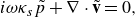 \begin{equation} i \omega \kappa _s \tilde {p} + \nabla \cdot \tilde {\mathbf{v}} = 0,\end{equation}
 \begin{equation} i \omega \bar {\rho } \tilde {\mathbf{v}} = - \nabla \tilde {p} + \mu \nabla ^2 \tilde {\mathbf{v}} + \mu \beta \nabla (\nabla \cdot \tilde {\mathbf{v}}). \end{equation}
In the above, $\kappa _s$
is the isentropic compressibility and it is correlated with the isothermal compressibility,
$\kappa _s$
is the isentropic compressibility and it is correlated with the isothermal compressibility, $\kappa _T$
, as
$\kappa _T$
, as $\kappa _T = \gamma \kappa _s$
, where
$\kappa _T = \gamma \kappa _s$
, where $\gamma = 1 + {\alpha _p^2 \bar {T}}/{\kappa _s \bar {\rho } c_p}$
is the ratio of specific heat capacities.
$\gamma = 1 + {\alpha _p^2 \bar {T}}/{\kappa _s \bar {\rho } c_p}$
is the ratio of specific heat capacities.
4. Numerical model
Our objective is to achieve a comprehensive understanding of acoustothermal heating, which necessitates determining the acoustic fields by solving (3.8) with the relevant boundary conditions. The material parameters used in this study are listed in § S3 of the Supplementary Material, where properties of the water have been taken from the COMSOL material library. Upon obtaining the acoustic fields, we can proceed to solve (3.5) to derive the acoustic streaming and the resultant acoustothermal temperature profile.
4.1. Computation of the acoustic fields
Solving for the acoustic response in our droplet system presents significant challenges, as the thicknesses of the acoustic viscous ( $\delta _{{vis}} = \sqrt {{(2 \mu)}/{(\omega \rho)}}$
) and thermal (
$\delta _{{vis}} = \sqrt {{(2 \mu)}/{(\omega \rho)}}$
) and thermal ( $\delta _{{th}} = \sqrt {{(2 D_{{th}})}/{\omega }}$
) boundary layers are much smaller than the SAW wavelength (
$\delta _{{th}} = \sqrt {{(2 D_{{th}})}/{\omega }}$
) boundary layers are much smaller than the SAW wavelength ( $\lambda$
), rendering a direct solution of (3.8) highly complex. To address this, we adopted similar methodologies as outlined in prior research (Das & Bhethanabotla Reference Das and Bhethanabotla2023), expressing
$\lambda$
), rendering a direct solution of (3.8) highly complex. To address this, we adopted similar methodologies as outlined in prior research (Das & Bhethanabotla Reference Das and Bhethanabotla2023), expressing $\tilde {\mathbf{v}} = \tilde {\mathbf{v}}_d + \tilde {\mathbf{v}}_\delta$
, where
$\tilde {\mathbf{v}} = \tilde {\mathbf{v}}_d + \tilde {\mathbf{v}}_\delta$
, where $\tilde {\mathbf{v}}_d$
and
$\tilde {\mathbf{v}}_d$
and $\tilde {\mathbf{v}}_\delta$
represent the long-range and short-range acoustic velocities associated with the scalar and the vector potentials, respectively. The corresponding temperature and pressure fields are similarly denoted by subscripts
$\tilde {\mathbf{v}}_\delta$
represent the long-range and short-range acoustic velocities associated with the scalar and the vector potentials, respectively. The corresponding temperature and pressure fields are similarly denoted by subscripts $d$
and
$d$
and $\delta$
. This approach culminates in a pressure acoustic model that yields
$\delta$
. This approach culminates in a pressure acoustic model that yields
 \begin{equation} \nabla ^2 \tilde {p}_d = - k_{{wave}}^2 \tilde {p}_d,\end{equation}
where $k_{{wave}} = k_0 (1 + i \Gamma)^{-1/2}$
is the effective acoustic wavenumber in the fluid;
$k_{{wave}} = k_0 (1 + i \Gamma)^{-1/2}$
is the effective acoustic wavenumber in the fluid; $k_0 = {\omega }/{c_0}$
is the wavenumber of the unattenuated wave in the fluid;
$k_0 = {\omega }/{c_0}$
is the wavenumber of the unattenuated wave in the fluid; $\Gamma = \omega (1 + \beta) \mu \kappa _s$
is the damping factor associated with viscous effects. The long-range acoustic velocity is related to the long-range acoustic pressure (
$\Gamma = \omega (1 + \beta) \mu \kappa _s$
is the damping factor associated with viscous effects. The long-range acoustic velocity is related to the long-range acoustic pressure ( $\tilde {p}_d$
) as
$\tilde {p}_d$
) as
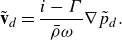 \begin{equation} \tilde {\mathbf{v}}_d = \frac {i - \Gamma }{\bar {\rho } \omega } \nabla \tilde {p}_d. \end{equation}
The boundary conditions associated with (4.1) are specified as (see Das & Bhethanabotla Reference Das and Bhethanabotla2023)
(i) at the bottom
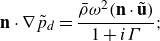 \begin{equation} \mathbf{n} \cdot \nabla \tilde {p}_d = \frac {\bar {\rho } \omega ^2 (\mathbf{n} \cdot \tilde {\mathbf{u}})}{1 + i \Gamma }; \end{equation}
(ii) at the free surface
 \begin{equation} \tilde {p}_d = 0.\end{equation}
The short-range velocity can be obtained as $\tilde {\mathbf{v}}_\delta = \tilde {\mathbf{v}}_b e^{-i k_v z}$
, where
$\tilde {\mathbf{v}}_\delta = \tilde {\mathbf{v}}_b e^{-i k_v z}$
, where $\tilde {\mathbf{v}}_b = {\partial \tilde {\mathbf{u}}}/{\partial t}$
and
$\tilde {\mathbf{v}}_b = {\partial \tilde {\mathbf{u}}}/{\partial t}$
and $k_v$
is the shear wavenumber, given by
$k_v$
is the shear wavenumber, given by $k_v = (1 - i)/\delta _{{vis}}$
. Furthermore, simulating the pressure acoustic model for our droplet system necessitates substantial computational resources due to the vast discrepancy between the droplet size and the SAW wavelength. To mitigate this, we decomposed the acoustic problem into a series of 2-D axisymmetric sub-problems, utilising cylindrical functions to represent the acoustic actuations. For that, we first expressed the SAW normal displacement function
$k_v = (1 - i)/\delta _{{vis}}$
. Furthermore, simulating the pressure acoustic model for our droplet system necessitates substantial computational resources due to the vast discrepancy between the droplet size and the SAW wavelength. To mitigate this, we decomposed the acoustic problem into a series of 2-D axisymmetric sub-problems, utilising cylindrical functions to represent the acoustic actuations. For that, we first expressed the SAW normal displacement function $ \hat {u}_z (x,y) \equiv \tilde {\mathbf{u}} \cdot \mathbf{e}_z e^{-i \omega t}$
in cylindrical coordinates
$ \hat {u}_z (x,y) \equiv \tilde {\mathbf{u}} \cdot \mathbf{e}_z e^{-i \omega t}$
in cylindrical coordinates $ \hat {u}_z (r,\theta)$
, which was then represented as a series of weighted exponential functions
$ \hat {u}_z (r,\theta)$
, which was then represented as a series of weighted exponential functions
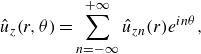 \begin{equation} \hat {u}_z (r, \theta) = \sum _{n = -\infty }^{+\infty } \hat {u}_{zn} (r) e^{in\theta }, \end{equation}
where $\hat {u}_{zn} (r)$
is given by
$\hat {u}_{zn} (r)$
is given by
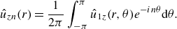 \begin{equation} \hat {u}_{zn} (r) = \frac {1}{2\pi } \int _{-\pi }^{\pi } \hat {u}_{1z} (r,\theta) e^{-in\theta } {\rm d}\theta.\end{equation}
We then express the acoustic pressure field in the form: $\hat {p}_d (r, \theta, z) = \hat {p}_n (r, z) e^{in\theta }$
and subsequently formulate our pressure acoustic equation (4.1) in the cylindrical coordinate system as
$\hat {p}_d (r, \theta, z) = \hat {p}_n (r, z) e^{in\theta }$
and subsequently formulate our pressure acoustic equation (4.1) in the cylindrical coordinate system as
 \begin{equation} \frac {1}{r} \frac {\partial \hat {p}_n}{\partial r} + \frac {\partial ^2 \hat {p}_n}{\partial r^2} + \frac {\partial ^2 \hat {p}_n}{\partial z^2} = \left ( \frac {n^2}{r^2} - k_{{wave}}^2 \right) \hat {p}_n \end{equation}
The boundary conditions associated with (4.5) become
(i) at the bottom
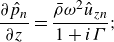 \begin{equation} \frac {\partial \hat {p}_n}{\partial z} = \frac {\bar {\rho } \omega ^2 \hat {u}_{zn}}{1 + i \Gamma }; \end{equation}
(ii) at the free surface
 \begin{equation} \hat {p}_n = 0.\end{equation}
Equation (4.5) along with associated boundary condition given by (4.6) are solved using finite element based commercial solver COMSOL Multiphysics. The solution can be reconstructed as
 \begin{equation} \hat {p}_d (r, \theta, z) = \sum _{n = -\infty }^{+\infty } \hat {p}_n (r, z) e^{in\theta }.\end{equation}
Once we obtain the long-range acoustic pressure, the long-range acoustic velocity can be calculated using (4.2).
4.2. Computation of the acoustothermal temperature profile
We now proceed to solve (3.5) to estimate the acoustothermal temperature field. As identified earlier, the mean velocity is significantly smaller than the oscillatory velocity fields (i.e. $\bar {\mathbf{v}}/\tilde {\mathbf{v}} = O(\tilde {\rho }/\bar {\rho }) \ll 1$
), allowing us to further neglect terms higher than
$\bar {\mathbf{v}}/\tilde {\mathbf{v}} = O(\tilde {\rho }/\bar {\rho }) \ll 1$
), allowing us to further neglect terms higher than $O[(\tilde {\rho }/\bar {\rho })^2]$
, reducing (3.5) to
$O[(\tilde {\rho }/\bar {\rho })^2]$
, reducing (3.5) to
 \begin{equation} \nabla \cdot (\langle \tilde {\rho } \tilde {\mathbf{v}} \rangle + \bar {\rho } \bar {\mathbf{v}}) = 0,\end{equation}
 \begin{equation} \bar {\rho } \partial _\tau \bar {\mathbf{v}} + \bar {\rho } (\bar {\mathbf{v}} \cdot \nabla) \bar {\mathbf{v}} = - \nabla \bar {p} + \mu \nabla ^2 \bar {\mathbf{v}} + \mu \beta \nabla (\nabla \cdot \bar {\mathbf{v}}) + \mathbf{F_{\textit{ac}}},\end{equation}
 \begin{equation} \bar {\rho } c_p \partial _\tau \bar {T} + (\bar {\rho } \bar {\mathbf{v}} + \langle \tilde {\rho } \tilde {\mathbf{v}} \rangle) c_p \cdot \nabla \bar {T} - \nabla \cdot (k_{{th}} \nabla \bar {T}) = \langle q_{\textit{ac}} \rangle,\end{equation}
where the acoustic body force is given by $\mathbf{F_{\textit{ac}}} = -\langle \tilde {\rho } \partial _t \tilde {\mathbf{v}} \rangle - \bar {\rho } \langle (\tilde {\mathbf{v}} \cdot \nabla) \tilde {\mathbf{v}} \rangle$
, and the acoustothermal heat source is expressed as
$\mathbf{F_{\textit{ac}}} = -\langle \tilde {\rho } \partial _t \tilde {\mathbf{v}} \rangle - \bar {\rho } \langle (\tilde {\mathbf{v}} \cdot \nabla) \tilde {\mathbf{v}} \rangle$
, and the acoustothermal heat source is expressed as
 \begin{equation} \langle q_{\textit{ac}} \rangle = \nabla \cdot [\langle \tilde {\mathbf{v}} \cdot \tilde {\boldsymbol{\sigma }} \rangle - \langle \mathbf{\Pi _{\textit{ac}}} \rangle], \end{equation}
where $ \langle \mathbf{\Pi _{\textit{ac}}} \rangle = \langle \tilde {p} \tilde {\mathbf{v}} \rangle$
is the Poynting vector, indicating the time-averaged acoustic energy flux in a spatial region. It is important to note that
$ \langle \mathbf{\Pi _{\textit{ac}}} \rangle = \langle \tilde {p} \tilde {\mathbf{v}} \rangle$
is the Poynting vector, indicating the time-averaged acoustic energy flux in a spatial region. It is important to note that $ \langle \tilde {\rho } \tilde {\mathbf{v}} \rangle c_p \cdot \nabla \bar {T}$
has not been included in the heat source term, as it primarily facilitates convective heat transport. Moreover, interestingly, in acoustothermal heating, the contribution of the term
$ \langle \tilde {\rho } \tilde {\mathbf{v}} \rangle c_p \cdot \nabla \bar {T}$
has not been included in the heat source term, as it primarily facilitates convective heat transport. Moreover, interestingly, in acoustothermal heating, the contribution of the term $ \nabla \cdot \langle \tilde {\mathbf{v}} \cdot \tilde {\boldsymbol{\sigma }} \rangle$
is negligibly small, as elucidated in our previous study (Das, Snider & Bhethanabotla Reference Das, Snider and Bhethanabotla2019) and also in § S5 of the Supplementary Material, reducing the heat source term to
$ \nabla \cdot \langle \tilde {\mathbf{v}} \cdot \tilde {\boldsymbol{\sigma }} \rangle$
is negligibly small, as elucidated in our previous study (Das, Snider & Bhethanabotla Reference Das, Snider and Bhethanabotla2019) and also in § S5 of the Supplementary Material, reducing the heat source term to
 \begin{equation} \langle q_{\textit{ac}} \rangle = -\nabla \cdot \langle \mathbf{\Pi _{\textit{ac}}} \rangle.\end{equation}
We further delve into characterising the acoustothermal heat source term and obtained the following closed-form expression (see Appendix A):
 \begin{equation} \langle q_{\textit{ac}} \rangle = \Gamma \bar {\rho } \omega \langle \tilde {\mathbf{v}} \cdot \tilde {\mathbf{v}} \rangle.\end{equation}
This is our main result and it depicts that the acoustothermal effect, observed over the slow time scale, is solely attributed to the power loss due to viscous damping. Note here that, for the large systems, where fluid domain size is much larger than the acoustic wavelength, the calculation of the divergence of the Poynting vector is a seemingly impossible task even with a modern computational facility. Hence, it is essential to use the closed form specified by (4.11) for the heating calculation.
It is important to specify here that (4.8a
–4.8b
), governing the mean flow, must be solved in conjunction with (4.8c
), as the acoustic streaming plays a pivotal role in convective heat transport within a sessile droplet. The calculation of the mean flow presents a formidable challenge due to the complexities associated with estimating the acoustic body force term in systems substantially larger than the acoustic wavelength. To alleviate the issues, we employed the well-established limiting velocity method (Chen et al. Reference Chen, Zhang, Mao, Nama, Gu, Huang, Jing, Guo, Costanzo and Huang2018), where the limiting velocity is prescribed at the droplet’s base and the slip wall condition is prescribed at the free surface. To solve the energy equation, at the droplet base we consider, $ \bar {T} = T_b$
, whereas, at the free surface, convective heat loss,
$ \bar {T} = T_b$
, whereas, at the free surface, convective heat loss, $ \mathbf{n} \cdot (-k_{{th}} \nabla \bar {T}) = h_{{amb}} (\bar {T} - T_0)$
is imposed.
$ \mathbf{n} \cdot (-k_{{th}} \nabla \bar {T}) = h_{{amb}} (\bar {T} - T_0)$
is imposed.
5. Results and discussion
5.1. Acoustic energy flow inside the sessile droplet
In our acoustothermal experiments, the sessile droplet is excited by the standing SAW generated on a lithium niobate piezoelectric substrate, exhibiting significant temperature rise. We have adopted a suitable coordinate system, as depicted in figure 1(a), wherein the origin is designated at the centre of the droplet base. In this configuration, the propagation of the standing SAW is aligned with the x-axis, while the z-axis denotes the direction orthogonal to the surface of the SAW device. When the standing SAW, propagating along the surface of the lithium niobate substrate, comes into contact with the droplet, it refracts into the droplet at a Rayleigh angle $ \theta _R \approx 22^\circ$
, due to the disparity in the speed of sound between the fluid and the piezoelectric substrate. The propagation of the refracted wave in the droplet is accompanied by the interaction of the acoustic energy into the fluid, leading to the acoustothermal effect. A comprehensive analysis of this energy interaction involved in the acoustothermal mechanism is elucidated in the ensuing sections.
$ \theta _R \approx 22^\circ$
, due to the disparity in the speed of sound between the fluid and the piezoelectric substrate. The propagation of the refracted wave in the droplet is accompanied by the interaction of the acoustic energy into the fluid, leading to the acoustothermal effect. A comprehensive analysis of this energy interaction involved in the acoustothermal mechanism is elucidated in the ensuing sections.
Note here that, albeit that the exchange of the acoustic energy occurs over a fast time scale, the acoustothermal temperature rise manifests over a slow time scale ( $\sim 10$
s), as evident from the experimental temperature profiles (figure 1
b–c). For a comprehensive characterisation of the acoustothermal effect, we first delved into the details of the acoustic field dynamics and identified the origin of the acoustothermal heat source. It is already well established that the acoustic–fluid interactions generate strong acoustic fields which harmonically oscillate over a fast time scale and, if we disregard the initial transience, the acoustic fields in the stable oscillation regime can be calculated theoretically or numerically.
$\sim 10$
s), as evident from the experimental temperature profiles (figure 1
b–c). For a comprehensive characterisation of the acoustothermal effect, we first delved into the details of the acoustic field dynamics and identified the origin of the acoustothermal heat source. It is already well established that the acoustic–fluid interactions generate strong acoustic fields which harmonically oscillate over a fast time scale and, if we disregard the initial transience, the acoustic fields in the stable oscillation regime can be calculated theoretically or numerically.
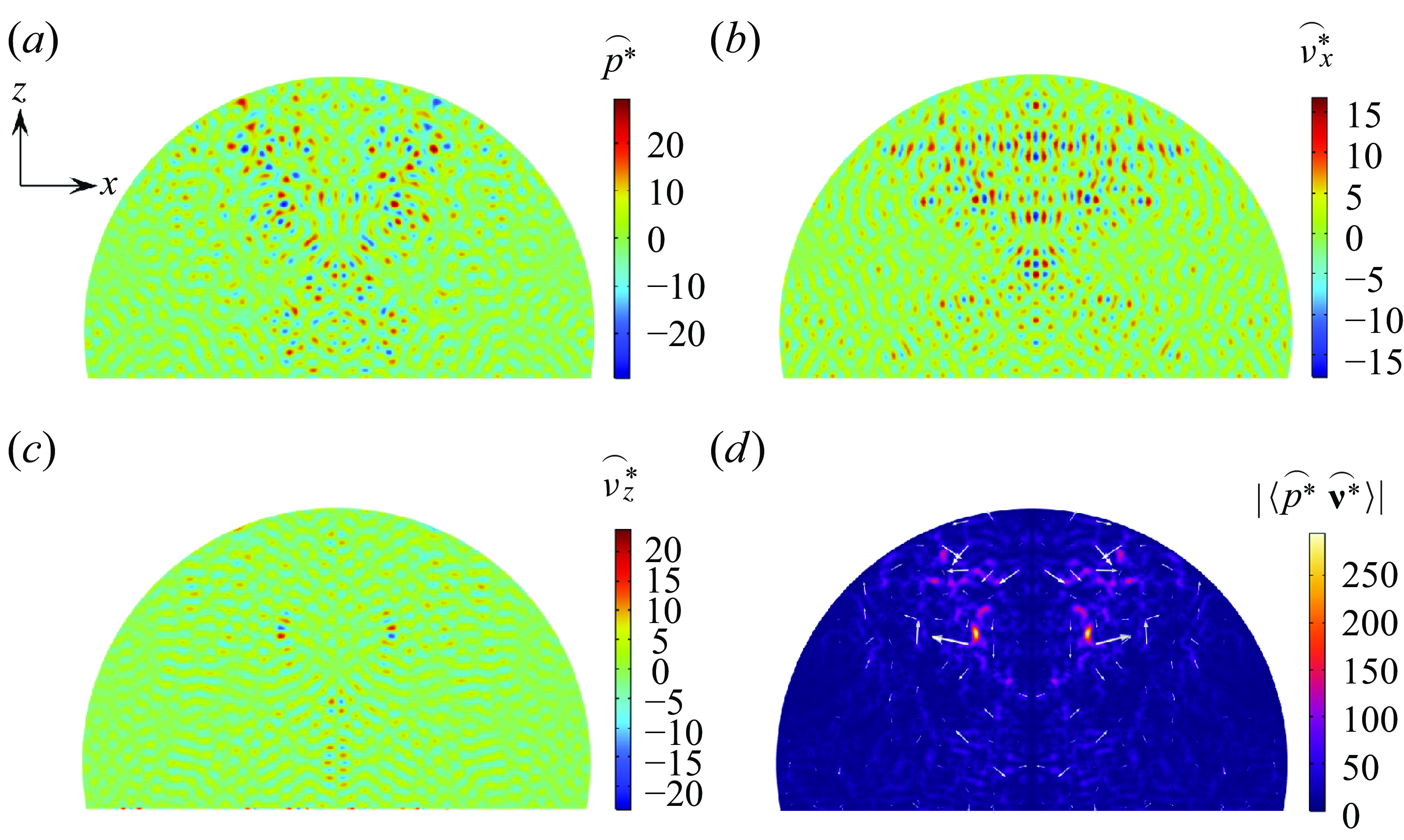
Figure 2. Acoustic energy flow inside a $2 \, \unicode{x03BC} \text{l}$
sessile droplet actuated by a
$2 \, \unicode{x03BC} \text{l}$
sessile droplet actuated by a $32.016 \, \text{MHz}$
standing SAW. Distribution of the acoustic pressure
$32.016 \, \text{MHz}$
standing SAW. Distribution of the acoustic pressure $(a)$
and the velocity fields
$(a)$
and the velocity fields $(b-c)$
along the meridian plane
$(b-c)$
along the meridian plane $(y = 0)$
. The magnitude of the time-averaged acoustic energy flux
$(y = 0)$
. The magnitude of the time-averaged acoustic energy flux $(d)$
shows the acoustic power flow inside the droplet. Two eyes are observed along the meridian plane, corresponding to the maximum power flow regions. A 3-D view of the two eyes is depicted in figure S3, see the supplementary material.
$(d)$
shows the acoustic power flow inside the droplet. Two eyes are observed along the meridian plane, corresponding to the maximum power flow regions. A 3-D view of the two eyes is depicted in figure S3, see the supplementary material.
Given that we have employed Fourier transform techniques to compute the acoustic fields, before presenting the acoustic field distribution results, it is crucial to scrutinise the accuracy of the method (see Appendix B). We found excellent agreement between the computed and the actual displacement fields, having variations of less than 2 %. Figure 2 illustrates the acoustic pressure and velocity fields, along with the acoustic energy flux, to elucidate the fluid–acoustic interactions over a fast time scale. As a standing SAW is propagating along the x-direction, we plotted acoustic fields along the meridian cross-section ( $y=0$
). Furthermore, the fields are expressed in dimensionless form,
$y=0$
). Furthermore, the fields are expressed in dimensionless form, $\hat {p}^* = {\hat {p}}/{\bar {\rho } c_0 u_0 \omega },\ \hat {\mathbf{v}}^* = {\hat {\mathbf{v}}}/{u_0 \omega }$
, to effectively generalise the representation, since the acoustic pressure and velocity fields are proportional to the amplitude of the SAW displacement. Because of the symmetry associated with acoustic actuations, the acoustic fields are symmetrical about the meridian plane (
$\hat {p}^* = {\hat {p}}/{\bar {\rho } c_0 u_0 \omega },\ \hat {\mathbf{v}}^* = {\hat {\mathbf{v}}}/{u_0 \omega }$
, to effectively generalise the representation, since the acoustic pressure and velocity fields are proportional to the amplitude of the SAW displacement. Because of the symmetry associated with acoustic actuations, the acoustic fields are symmetrical about the meridian plane ( $y=0$
). However, an antisymmetric pressure distribution is observed along the
$y=0$
). However, an antisymmetric pressure distribution is observed along the $x=0$
plane (figure 2
a), which is attributed to the antisymmetric SAW displacement field, as evident from (3.2a
). Figure 2(b)–2(c) show that the dimensionless acoustic velocity,
$x=0$
plane (figure 2
a), which is attributed to the antisymmetric SAW displacement field, as evident from (3.2a
). Figure 2(b)–2(c) show that the dimensionless acoustic velocity, $\hat {\mathbf{v}}^*$
, exhibits values much higher than unity, implying a substantial number of acoustic wave reflections at the dropletair interface. These reflections increase the acoustic velocity due to enhanced acoustic–fluid interactions associated with the significantly large wave propagation paths.
$\hat {\mathbf{v}}^*$
, exhibits values much higher than unity, implying a substantial number of acoustic wave reflections at the dropletair interface. These reflections increase the acoustic velocity due to enhanced acoustic–fluid interactions associated with the significantly large wave propagation paths.
The acoustic energy flux distribution is observed to be symmetrical and shows a few hot spots with two prominent eyes near the droplet centroid (figure 2 d), which result from the overlap of the reflection pathways of the longitudinal acoustic waves as they reflect multiple times on the droplet–air interface and the SAW surface. The arrows indicate the direction of the power flow and it is observed to be outward in a circular fashion, leading to enhanced energy dissipation into the fluid. Note here that these two eyes are only present along the meridian plane and do not appear anywhere else (see § S4 in the Supplementary Material).
5.2. Acoustothermal mechanism
To delve into the intricacies of the heating mechanism, we commence by scrutinising the heat source term delineated in (4.11). The divergence of the acoustic energy flux can be expressed, in its non-time-averaged form, as follows:
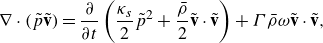 \begin{equation} \nabla \cdot (\tilde {p} \tilde {\mathbf{v}}) = \frac {\partial }{\partial t} \left ( \frac {\kappa _s}{2} \tilde {p}^2 + \frac {\bar {\rho }}{2} \tilde {\mathbf{v}} \cdot \tilde {\mathbf{v}} \right) + \Gamma \bar {\rho } \omega \tilde {\mathbf{v}} \cdot \tilde {\mathbf{v}}, \end{equation}
where ${\kappa _s}/{2} (\tilde {p}^2$
) and
${\kappa _s}/{2} (\tilde {p}^2$
) and ${\bar {\rho }}/{2} (\tilde {\mathbf{v}} \cdot \tilde {\mathbf{v}})$
represent the acoustic pressure energy density (
${\bar {\rho }}/{2} (\tilde {\mathbf{v}} \cdot \tilde {\mathbf{v}})$
represent the acoustic pressure energy density ( $E_{p,{ac}}$
) and the kinetic energy density (
$E_{p,{ac}}$
) and the kinetic energy density ( $E_{v,{ac}}$
), respectively. The transfer of acoustic energy into the fluid is thus characterised by the rate of change in acoustic energy density and the losses associated with damping due to fluid viscous effects. The time-averaged values of the acoustic energy density are calculated to be zero since
$E_{v,{ac}}$
), respectively. The transfer of acoustic energy into the fluid is thus characterised by the rate of change in acoustic energy density and the losses associated with damping due to fluid viscous effects. The time-averaged values of the acoustic energy density are calculated to be zero since $\langle \tilde {p} i \tilde {p} \rangle$
and
$\langle \tilde {p} i \tilde {p} \rangle$
and $\langle \tilde {\mathbf{v}} \cdot i \tilde {\mathbf{v}} \rangle$
are zero.
$\langle \tilde {\mathbf{v}} \cdot i \tilde {\mathbf{v}} \rangle$
are zero.
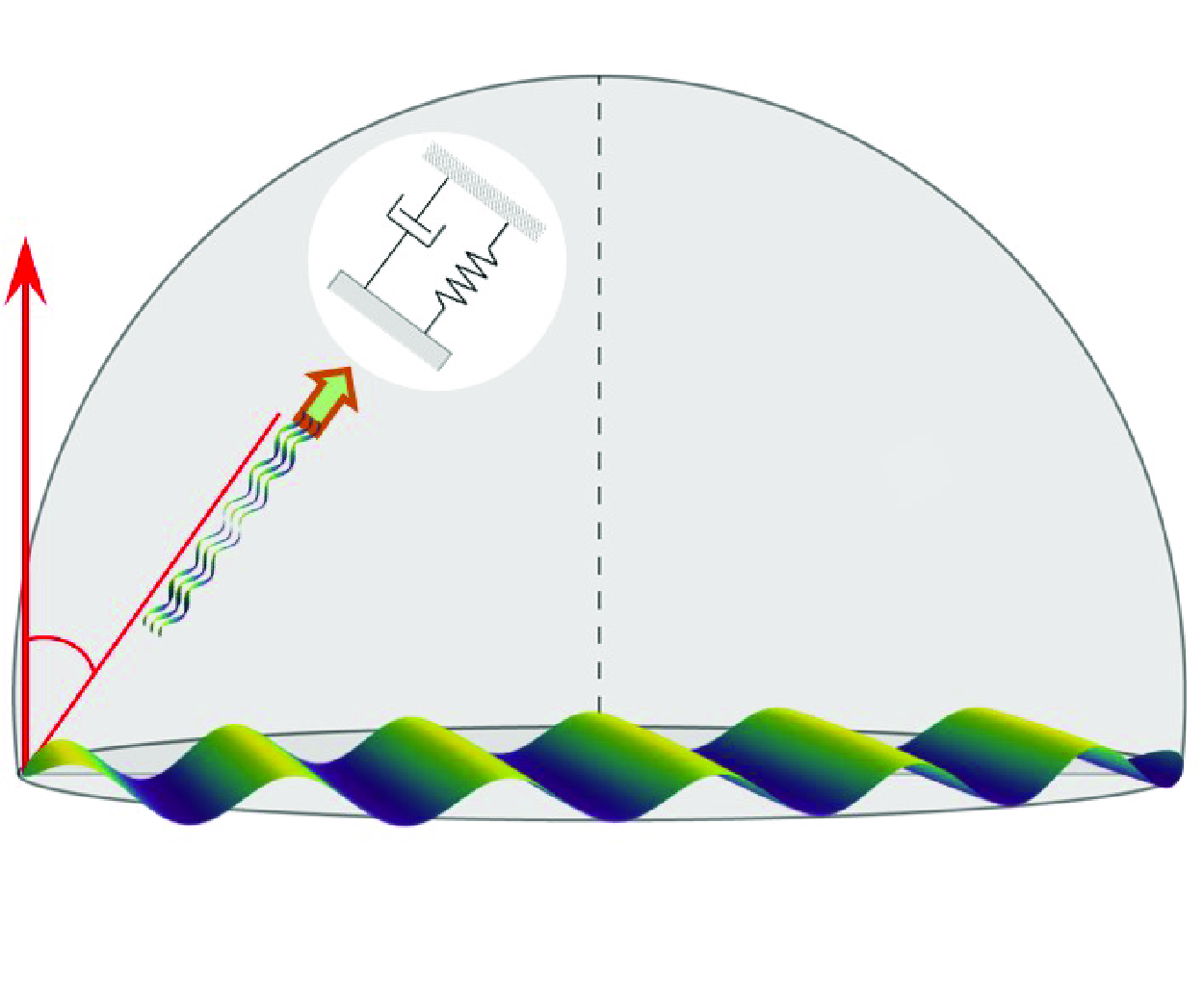
Evidently, the closed-form acoustothermal heat source expression elucidates that it is proportional to the viscous damping factor, thereby revealing direct correlations with both the shear and bulk viscosities. Furthermore, it delineates the exact parameters and variables instrumental in the acoustothermal effect. The acoustothermal mechanism can be effectively illustrated by the spring-dashpot system wherein the fluctuations of acoustic energy density can be conceptualised as analogous to a spring system, while the viscous damping is epitomised by the dashpot system (figure 3).
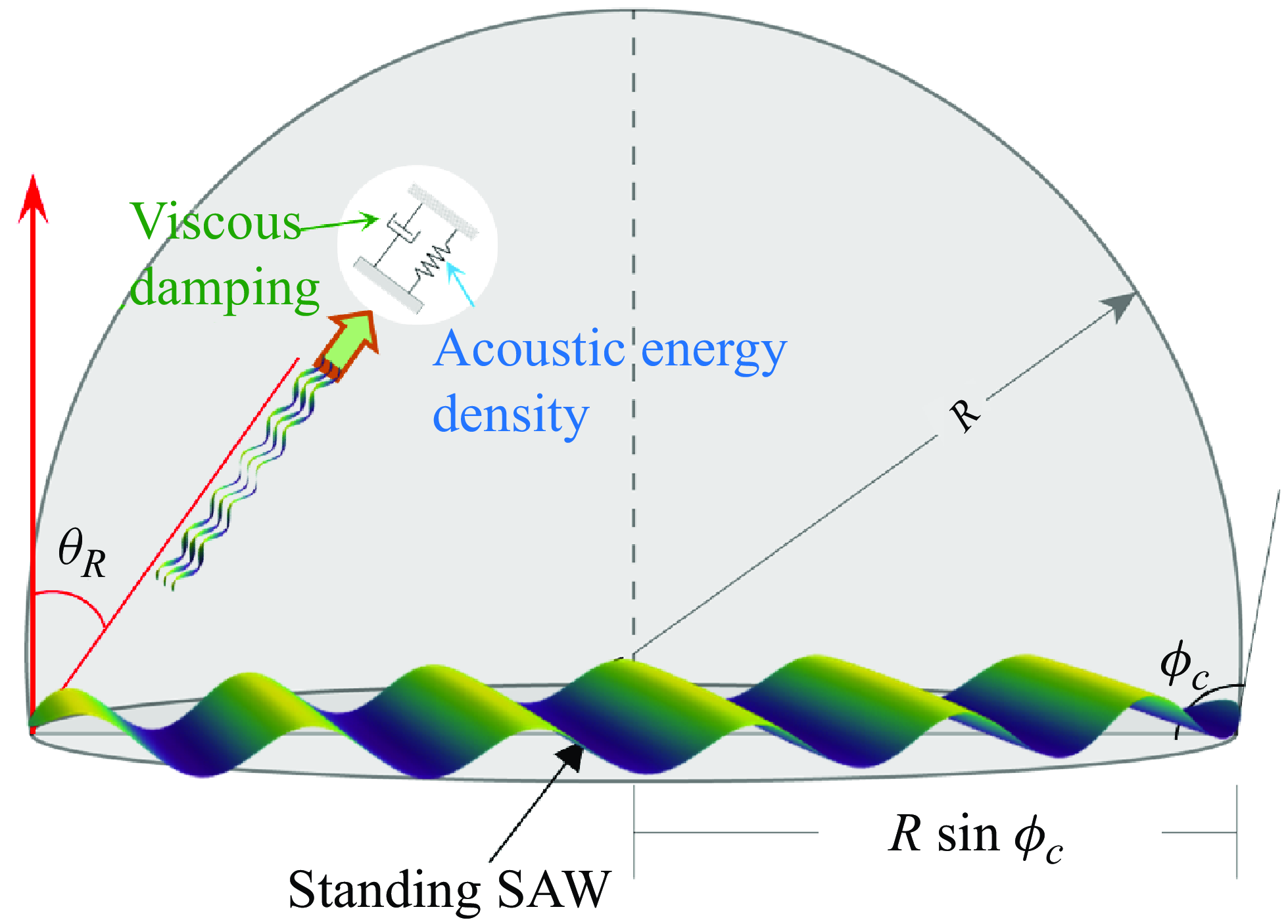
Figure 3. Schematic illustrating standing SAW-mediated acoustothermal mechanism due to the dissipation of the acoustic energy into the droplet. The acoustothermal mechanism is effectively represented by a spring-dashpot model, where fluctuations in acoustic energy density are analogous to the behaviour of a spring, and viscous damping is symbolised by the action of a dashpot.
As mentioned, the acoustothermal heat source is primarily characterised by the divergence of the acoustic energy flux and subsequently, the total heat generation is obtained by integrating it over the droplet volume
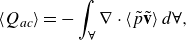 \begin{equation} \langle Q_{\textit{ac}} \rangle = -\int _\forall \nabla \cdot \langle \tilde {p} \tilde {\mathbf{v}} \rangle \, d\forall,\end{equation}
where $\forall$
denotes the volume of the droplet. Utilising the divergence theorem, the heat source can be rewritten as
$\forall$
denotes the volume of the droplet. Utilising the divergence theorem, the heat source can be rewritten as $\langle Q_{\textit{ac}} \rangle = -\oint _{\partial \Omega } \langle \tilde {p} \tilde {\mathbf{v}} \rangle \cdot \mathbf{n} \, {\rm d}s$
, where
$\langle Q_{\textit{ac}} \rangle = -\oint _{\partial \Omega } \langle \tilde {p} \tilde {\mathbf{v}} \rangle \cdot \mathbf{n} \, {\rm d}s$
, where $\partial \Omega$
is the closed surface of the sessile droplet. Since we consider the acoustic pressure,
$\partial \Omega$
is the closed surface of the sessile droplet. Since we consider the acoustic pressure, $\tilde {p}$
, to be zero at the free surface, the acoustothermal heat rate is the power transmitted into the droplet from the droplet bottom (denoted by
$\tilde {p}$
, to be zero at the free surface, the acoustothermal heat rate is the power transmitted into the droplet from the droplet bottom (denoted by $\partial \Omega _b$
), i.e.
$\partial \Omega _b$
), i.e.
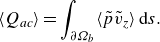 \begin{equation} \langle Q_{\textit{ac}} \rangle = \int _{\partial \Omega _b} \langle \tilde {p} \tilde {v}_z \rangle \, {\rm d}s.\end{equation}
This fundamentally signifies that acoustic energy is absorbed at the droplet’s base, where the standing SAW meets with the fluid. Note here that this phenomenon of the absorption of sound in lossy media such as fluids, has been the subject of interest for many decades. The incident acoustic energy flux from the droplet’s base, when propagating inside the fluids, loses its energy, facilitating the fluids to absorb the acoustic energy. The attenuation of the acoustic intensity ( $\mathbf{I}_a$
) inside the fluids follows the relationship
$\mathbf{I}_a$
) inside the fluids follows the relationship $\mathbf{I}_a = \mathbf{I}_0 e^{-2\alpha |\mathbf{r}|}$
, where
$\mathbf{I}_a = \mathbf{I}_0 e^{-2\alpha |\mathbf{r}|}$
, where $\mathbf{r} = |\mathbf{r}| \mathbf{e}_r$
is the position vector (
$\mathbf{r} = |\mathbf{r}| \mathbf{e}_r$
is the position vector ( $\mathbf{e}_r$
is the unit vector) at which the intensity
$\mathbf{e}_r$
is the unit vector) at which the intensity $\mathbf{I}_a$
is defined, and
$\mathbf{I}_a$
is defined, and $\mathbf{I_0}$
is the intensity at the source (i.e.
$\mathbf{I_0}$
is the intensity at the source (i.e. $\mathbf{r} = 0$
). With the seminal theory first provided by Stokes in 1845 (Stokes Reference Stokes2009), a substantial corpus of literature has traditionally attributed acoustic attenuation in fluids solely to shear viscosity (attenuation coefficient
$\mathbf{r} = 0$
). With the seminal theory first provided by Stokes in 1845 (Stokes Reference Stokes2009), a substantial corpus of literature has traditionally attributed acoustic attenuation in fluids solely to shear viscosity (attenuation coefficient $\alpha = {2\omega ^2 \mu \kappa _s}/{3c_0}$
), leveraging translational relaxation of the molecular degrees of freedom. Later, researchers modified the attenuation coefficient as
$\alpha = {2\omega ^2 \mu \kappa _s}/{3c_0}$
), leveraging translational relaxation of the molecular degrees of freedom. Later, researchers modified the attenuation coefficient as $\alpha = {\omega \Gamma }/{2c_0}$
, elucidating an additional mechanism of energy dissipation via vibrational, rotational and molecular conformation relaxation, attributable to the bulk viscosity of the fluid (Temkin Reference Temkin1981). Therefore, the attenuation of the acoustic energy depends on the viscous damping coefficient
$\alpha = {\omega \Gamma }/{2c_0}$
, elucidating an additional mechanism of energy dissipation via vibrational, rotational and molecular conformation relaxation, attributable to the bulk viscosity of the fluid (Temkin Reference Temkin1981). Therefore, the attenuation of the acoustic energy depends on the viscous damping coefficient $\Gamma$
, which has
$\Gamma$
, which has $4/3:1$
contributions from shear viscosity and bulk viscosity.
$4/3:1$
contributions from shear viscosity and bulk viscosity.
Earlier, we specified that the term $\nabla \cdot \langle \tilde {\mathbf{v}} \cdot \tilde {\boldsymbol{\sigma }} \rangle$
is negligibly small in contributing as the acoustothermal heat source. Nevertheless, the term can be expanded as
$\nabla \cdot \langle \tilde {\mathbf{v}} \cdot \tilde {\boldsymbol{\sigma }} \rangle$
is negligibly small in contributing as the acoustothermal heat source. Nevertheless, the term can be expanded as $\langle \tilde {\mathbf{v}} \cdot (\nabla \cdot \tilde {\boldsymbol{\sigma }}) \rangle + \langle \nabla \tilde {\mathbf{v}}: \tilde {\boldsymbol{\sigma }} \rangle$
and, by employing (3.8b
), one can reformulate (4.9), without time averaging, as (see Appendix C)
$\langle \tilde {\mathbf{v}} \cdot (\nabla \cdot \tilde {\boldsymbol{\sigma }}) \rangle + \langle \nabla \tilde {\mathbf{v}}: \tilde {\boldsymbol{\sigma }} \rangle$
and, by employing (3.8b
), one can reformulate (4.9), without time averaging, as (see Appendix C)
 \begin{equation} q_{ac} = \frac {\partial }{\partial t} \left ( \frac {\kappa _s}{2} \tilde {p}^2 + \frac {\bar {\rho }}{2} \tilde {\mathbf{v}} \cdot \tilde {\mathbf{v}} \right) + (\nabla \tilde {\mathbf{v}}: \tilde {\boldsymbol{\sigma }}). \end{equation}
This is quite similar to (5.1), where the transfer of acoustic energy into the fluid is thus characterised by the oscillatory fluctuations of the acoustic energy density and the frictional losses due to fluid viscosity. Necessarily, the first term on the right-hand side, upon time averaging, becomes zero, leaving the heat source, $\langle q_{ac} \rangle$
, as the time-averaged viscous dissipation only. Given that, accurately estimating the viscous dissipation term
$\langle q_{ac} \rangle$
, as the time-averaged viscous dissipation only. Given that, accurately estimating the viscous dissipation term $\langle \nabla \tilde {\mathbf{v}}: \tilde {\boldsymbol{\sigma }} \rangle$
in large systems is exceedingly challenging, one needs to use the closed-form expression given by (4.11) instead of
$\langle \nabla \tilde {\mathbf{v}}: \tilde {\boldsymbol{\sigma }} \rangle$
in large systems is exceedingly challenging, one needs to use the closed-form expression given by (4.11) instead of $\langle \nabla \tilde {\mathbf{v}}: \tilde {\boldsymbol{\sigma }} \rangle$
to generalise the heat source for both small and large systems (see § S5 in the Supplementary Material).
$\langle \nabla \tilde {\mathbf{v}}: \tilde {\boldsymbol{\sigma }} \rangle$
to generalise the heat source for both small and large systems (see § S5 in the Supplementary Material).
5.3. Acoustothermal temperature distribution
In our experiments, a thermal camera was utilised to measure the droplet temperature from the top. The experiments were conducted at input power levels $P_{{SAW}} = 6.1, 18.5, 36.4, 59.4, 75.6, 91.9$
and
$P_{{SAW}} = 6.1, 18.5, 36.4, 59.4, 75.6, 91.9$
and $116.0 \, \text{mW}$
on each IDT side. So, the total power to the SAW device is given by
$116.0 \, \text{mW}$
on each IDT side. So, the total power to the SAW device is given by $P_{{SAW,t}} = 2P_{{SAW}}$
. Each experiment was repeated three times at each power level to ensure data reproducibility and to measure the standard deviations associated with the temperature measurements of the sessile droplets. Upon activation of the SAW (
$P_{{SAW,t}} = 2P_{{SAW}}$
. Each experiment was repeated three times at each power level to ensure data reproducibility and to measure the standard deviations associated with the temperature measurements of the sessile droplets. Upon activation of the SAW ( $\tau = 0$
), the droplet temperature exhibited a sharp initial increase, followed by a gradual rise until reaching a steady state. We observed some fluctuations in the droplet temperature as it approached the steady state, likely due to the small droplet size, which makes it susceptible to slight changes in the ambient conditions.
$\tau = 0$
), the droplet temperature exhibited a sharp initial increase, followed by a gradual rise until reaching a steady state. We observed some fluctuations in the droplet temperature as it approached the steady state, likely due to the small droplet size, which makes it susceptible to slight changes in the ambient conditions.
It is noteworthy that, in addition to acoustothermal effects, there are other heat generation sources such as Joule heating of IDTs and dielectric loss within piezoelectric substrates, responsible for the temperature rise of the droplet. Consequently, in our experimentally acquired dataset, the influence of substrate heating due to these extraneous heat sources is an inherent and unavoidable factor. This inherent thermal influence renders the decoupling of acoustothermal effects from extraneous heat sources an exceedingly formidable challenge. To address these thermal interferences, Shilton et al. (Reference Shilton2015) placed the SAW device on a thermally regulated aluminium chip carrier, maintaining it at ambient temperature (i.e. $T_b = T_0$
) via a Peltier cooling system. While this approach effectively minimised Joule heating and dielectric losses, ensuring the substrate remained at ambient temperature in the absence of a sessile droplet, it introduced a fundamental limitation: the Peltier cooling mechanism may inadvertently extract thermal energy from the acoustothermal heating of the droplet, thereby leading to an overall reduction in the droplet’s temperature rise. Although the influence of extraneous heat sources is relatively minor, it is imperative to acknowledge that even such ostensibly minor heating effects may exert a non-negligible influence on the overall thermal profile of a sessile droplet, as captured via the thermal camera.
$T_b = T_0$
) via a Peltier cooling system. While this approach effectively minimised Joule heating and dielectric losses, ensuring the substrate remained at ambient temperature in the absence of a sessile droplet, it introduced a fundamental limitation: the Peltier cooling mechanism may inadvertently extract thermal energy from the acoustothermal heating of the droplet, thereby leading to an overall reduction in the droplet’s temperature rise. Although the influence of extraneous heat sources is relatively minor, it is imperative to acknowledge that even such ostensibly minor heating effects may exert a non-negligible influence on the overall thermal profile of a sessile droplet, as captured via the thermal camera.
In the present study, we account for the effects of these extraneous heat sources by experimentally measuring the temperature of the SAW device in the absence of a droplet while the SAW was activated, thereby characterising the substrate heating. This results in an elevated substrate temperature, which ranged from $\sim$
0.2
$\sim$
0.2 $\,^\circ$
C to a peak value of
$\,^\circ$
C to a peak value of $\sim$
1
$\sim$
1 $\,^\circ$
C across our experimental conditions. We circumvented the challenges in precisely disentangling acoustothermal effects from extraneous heat sources by implementing a correction to the thermal camera dataset. This correction was achieved through numerical simulations, which quantified the variations in droplet temperature rise resulting from the elevated lithium niobate substrate temperature caused by extraneous heat sources. Consequently, the droplet temperature rise data have been adjusted to exclude heating effects from non-acoustothermal sources, thereby isolating the thermal profile solely attributable to acoustothermal effects (see § S6 in the Supplementary Material).
$\,^\circ$
C across our experimental conditions. We circumvented the challenges in precisely disentangling acoustothermal effects from extraneous heat sources by implementing a correction to the thermal camera dataset. This correction was achieved through numerical simulations, which quantified the variations in droplet temperature rise resulting from the elevated lithium niobate substrate temperature caused by extraneous heat sources. Consequently, the droplet temperature rise data have been adjusted to exclude heating effects from non-acoustothermal sources, thereby isolating the thermal profile solely attributable to acoustothermal effects (see § S6 in the Supplementary Material).
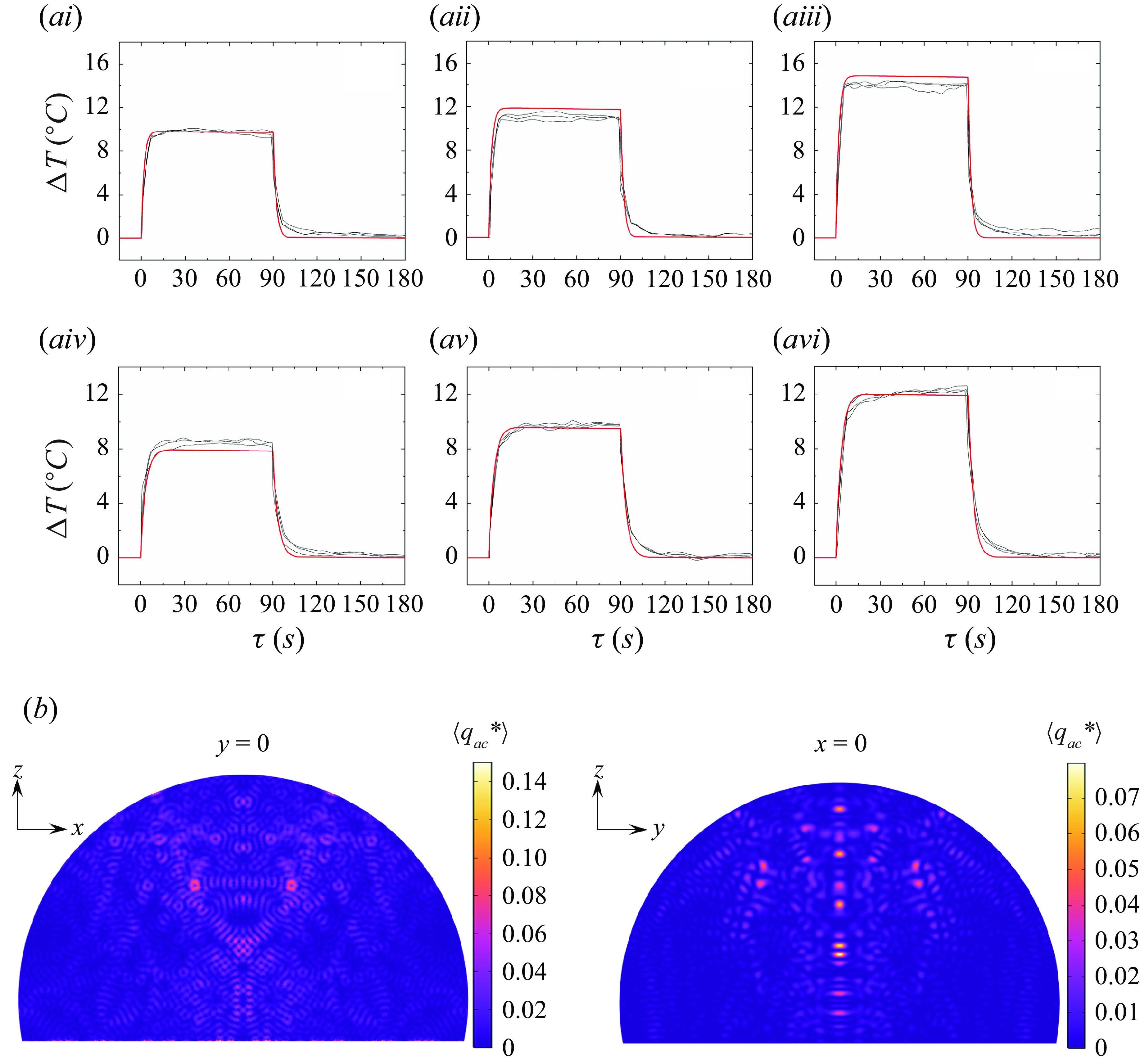
Figure 4. Acoustothermal dynamics and heat source. (a) The dynamics of the sessile droplet temperature rise, $\Delta T$
, as a function of time,
$\Delta T$
, as a function of time, $\tau$
, is shown for 2
$\tau$
, is shown for 2 $\unicode{x03BC}$
l (i–iii) and 5
$\unicode{x03BC}$
l (i–iii) and 5 $\unicode{x03BC}$
l (iv–vi) droplets at
$\unicode{x03BC}$
l (iv–vi) droplets at $P_{{SAW},t} = 151.3$
(i and iv), 183.7 (ii and v) and 232.0 (iii and vi) mW. Black lines represent experimental results, whereas the red line indicates numerical predictions. Experimental temperature rise data presented here have been corrected, accounting for no external heat source, and thereby resulting in
$P_{{SAW},t} = 151.3$
(i and iv), 183.7 (ii and v) and 232.0 (iii and vi) mW. Black lines represent experimental results, whereas the red line indicates numerical predictions. Experimental temperature rise data presented here have been corrected, accounting for no external heat source, and thereby resulting in $T_b = T_0$
. (b) Spatial distribution of the acoustothermal heat source is shown for a 2
$T_b = T_0$
. (b) Spatial distribution of the acoustothermal heat source is shown for a 2 $\unicode{x03BC}$
l droplet along meridian planes (
$\unicode{x03BC}$
l droplet along meridian planes ( $y = 0$
and
$y = 0$
and $x = 0$
). The maximum heat generation occurs around the two eyes, corresponding to the maximum Poynting vector magnitudes (see figure S3 in the supplementary material).
$x = 0$
). The maximum heat generation occurs around the two eyes, corresponding to the maximum Poynting vector magnitudes (see figure S3 in the supplementary material).
Rigorous numerical studies have been performed to obtain the acoustothermal dynamics. As the experimental data are corrected to exclude the external heat sources, the numerical simulations are conducted by assigning the droplet’s bottom temperature to the ambient temperature (i.e. $T_b = T_0$
). First, the acoustic pressure and velocity fields were determined and, thereafter, these fields were utilised to quantify the time-averaged acoustothermal heat source, which serves as the sole source for the acoustothermal effect. Figure 4(a) depicts the variation in droplet temperature,
$T_b = T_0$
). First, the acoustic pressure and velocity fields were determined and, thereafter, these fields were utilised to quantify the time-averaged acoustothermal heat source, which serves as the sole source for the acoustothermal effect. Figure 4(a) depicts the variation in droplet temperature, $\Delta T = (T_{{max}} - T_0)$
, as a function of time,
$\Delta T = (T_{{max}} - T_0)$
, as a function of time, $\tau$
, for
$\tau$
, for $2 $
and
$2 $
and $5 \, \unicode{x03BC} \text{l}$
droplets, as obtained through both numerical simulations (red lines) and experimental measurements (black lines). The numerical results accurately predict the acoustothermal dynamics, effectively capturing the underlying physics. Figure 4(
b) presents the distribution of the heat source, prescribed by (4.11), expressed in dimensionless form as
$5 \, \unicode{x03BC} \text{l}$
droplets, as obtained through both numerical simulations (red lines) and experimental measurements (black lines). The numerical results accurately predict the acoustothermal dynamics, effectively capturing the underlying physics. Figure 4(
b) presents the distribution of the heat source, prescribed by (4.11), expressed in dimensionless form as $\langle q_{ac}^* \rangle = \Gamma \langle \tilde {\mathbf{v}} \cdot \tilde {\mathbf{v}} \rangle$
for a
$\langle q_{ac}^* \rangle = \Gamma \langle \tilde {\mathbf{v}} \cdot \tilde {\mathbf{v}} \rangle$
for a $2 \, \unicode{x03BC} \text{l}$
droplet along meridian planes (
$2 \, \unicode{x03BC} \text{l}$
droplet along meridian planes ( $x=0$
and
$x=0$
and $y=0$
). The spatial distribution reveals that the maximum acoustothermal heat generation is observed to occur near the two ‘eyes’ associated with the maximum acoustic energy flux magnitude. It is noteworthy that the other equivalence of the heat source terms (4.9 and 4.10) has also been demonstrated both theoretically and numerically in the Supplementary Material. We have shown that the
$y=0$
). The spatial distribution reveals that the maximum acoustothermal heat generation is observed to occur near the two ‘eyes’ associated with the maximum acoustic energy flux magnitude. It is noteworthy that the other equivalence of the heat source terms (4.9 and 4.10) has also been demonstrated both theoretically and numerically in the Supplementary Material. We have shown that the $\nabla \cdot \langle \tilde {\mathbf{v}} \cdot \tilde {\boldsymbol{\sigma }} \rangle$
term in the heat source is negligibly small, and the heat is primarily generated due to the divergence of the Poynting vector.
$\nabla \cdot \langle \tilde {\mathbf{v}} \cdot \tilde {\boldsymbol{\sigma }} \rangle$
term in the heat source is negligibly small, and the heat is primarily generated due to the divergence of the Poynting vector.
Figure 5(a) depicts the maximum temperature rise as a function of input SAW power into the droplets of $2 $
and
$2 $
and $5 \, \unicode{x03BC} \text{l}$
. Here, symbols represent experimental results, while lines indicate numerical predictions. The inset of figure 5(a) shows the arrow plot of the acoustic streaming fields in sessile droplets (due to symmetry, only one quarter is shown). The acoustothermal temperature rise is, therefore, observed to vary linearly with the input SAW power. It is important to mention here that the present study considered input powers up to
$5 \, \unicode{x03BC} \text{l}$
. Here, symbols represent experimental results, while lines indicate numerical predictions. The inset of figure 5(a) shows the arrow plot of the acoustic streaming fields in sessile droplets (due to symmetry, only one quarter is shown). The acoustothermal temperature rise is, therefore, observed to vary linearly with the input SAW power. It is important to mention here that the present study considered input powers up to $P_{{SAW,t}} = 2P_{{SAW}} = 0.232 \, \text{W}$
, for which the convective heat transport (including the acoustic field-assisted convection) is not large enough to manoeuvre the temperature rise from linearity. However, it helps in enhancing the heat transport, thereby reducing the temperature rise slightly (
$P_{{SAW,t}} = 2P_{{SAW}} = 0.232 \, \text{W}$
, for which the convective heat transport (including the acoustic field-assisted convection) is not large enough to manoeuvre the temperature rise from linearity. However, it helps in enhancing the heat transport, thereby reducing the temperature rise slightly ( $\sim 2\,\,\%$
drop in
$\sim 2\,\,\%$
drop in $\Delta T$
). Experimentally, at
$\Delta T$
). Experimentally, at $P_{{SAW,t}} = 0.232 \, \text{W}$
, the maximum temperature rise for a
$P_{{SAW,t}} = 0.232 \, \text{W}$
, the maximum temperature rise for a $2 \, \unicode{x03BC} \text{l}$
droplet is observed to be
$2 \, \unicode{x03BC} \text{l}$
droplet is observed to be $14.08 \pm 0.6 \, ^\circ \text{C}$
, whereas for a
$14.08 \pm 0.6 \, ^\circ \text{C}$
, whereas for a $5 \, \unicode{x03BC} \text{l}$
droplet, the temperature rise is
$5 \, \unicode{x03BC} \text{l}$
droplet, the temperature rise is $12.27 \pm 0.32 \, ^\circ \text{C}$
, indicating a decrease in temperature rise with increasing droplet volume. Our theoretical estimations show a similar trend with a
$12.27 \pm 0.32 \, ^\circ \text{C}$
, indicating a decrease in temperature rise with increasing droplet volume. Our theoretical estimations show a similar trend with a $14.73 \, ^\circ \text{C}$
temperature rise for a
$14.73 \, ^\circ \text{C}$
temperature rise for a $2 \, \unicode{x03BC} \text{l}$
droplet and a
$2 \, \unicode{x03BC} \text{l}$
droplet and a $11.89 \, ^\circ \text{C}$
temperature rise for a
$11.89 \, ^\circ \text{C}$
temperature rise for a $5 \, \unicode{x03BC} \text{l}$
droplet. This can be attributed to the fact that, with an increase in volume, the amount of heat required to achieve the same temperature rise increases linearly, whereas the heat generation in droplets at the same input power level does not follow a linear trend. In fact, irrespective of the power level, a
$5 \, \unicode{x03BC} \text{l}$
droplet. This can be attributed to the fact that, with an increase in volume, the amount of heat required to achieve the same temperature rise increases linearly, whereas the heat generation in droplets at the same input power level does not follow a linear trend. In fact, irrespective of the power level, a $2 \, \unicode{x03BC} \text{l}$
droplet is able to convert
$2 \, \unicode{x03BC} \text{l}$
droplet is able to convert $16.46\,\%$
of the input power into acoustothermal heating, whereas in a
$16.46\,\%$
of the input power into acoustothermal heating, whereas in a $5 \, \unicode{x03BC} \text{l}$
droplet around
$5 \, \unicode{x03BC} \text{l}$
droplet around $17.05\,\%$
conversion of the input power is estimated. This constitutes merely a
$17.05\,\%$
conversion of the input power is estimated. This constitutes merely a $3.6\,\%$
increase in acoustic energy dissipation rate despite a
$3.6\,\%$
increase in acoustic energy dissipation rate despite a $150\,\%$
increase in droplet volume (and an
$150\,\%$
increase in droplet volume (and an $84.2\,\%$
increase in droplet base area from where the acoustic energy is absorbed). Figure 5(b) illustrates the steady-state temperature distribution inside the droplet under the influence of standing SAW actuation. Due to symmetry, only one quarter of the droplet is depicted. As the temperature rise,
$84.2\,\%$
increase in droplet base area from where the acoustic energy is absorbed). Figure 5(b) illustrates the steady-state temperature distribution inside the droplet under the influence of standing SAW actuation. Due to symmetry, only one quarter of the droplet is depicted. As the temperature rise, $(\bar {T} - T_0)$
, is proportional to the input SAW power, we presented the temperature distribution, scaled by the SAW power, for both
$(\bar {T} - T_0)$
, is proportional to the input SAW power, we presented the temperature distribution, scaled by the SAW power, for both $2 $
and
$2 $
and $5 \, \unicode{x03BC} \text{l}$
droplets.
$5 \, \unicode{x03BC} \text{l}$
droplets.
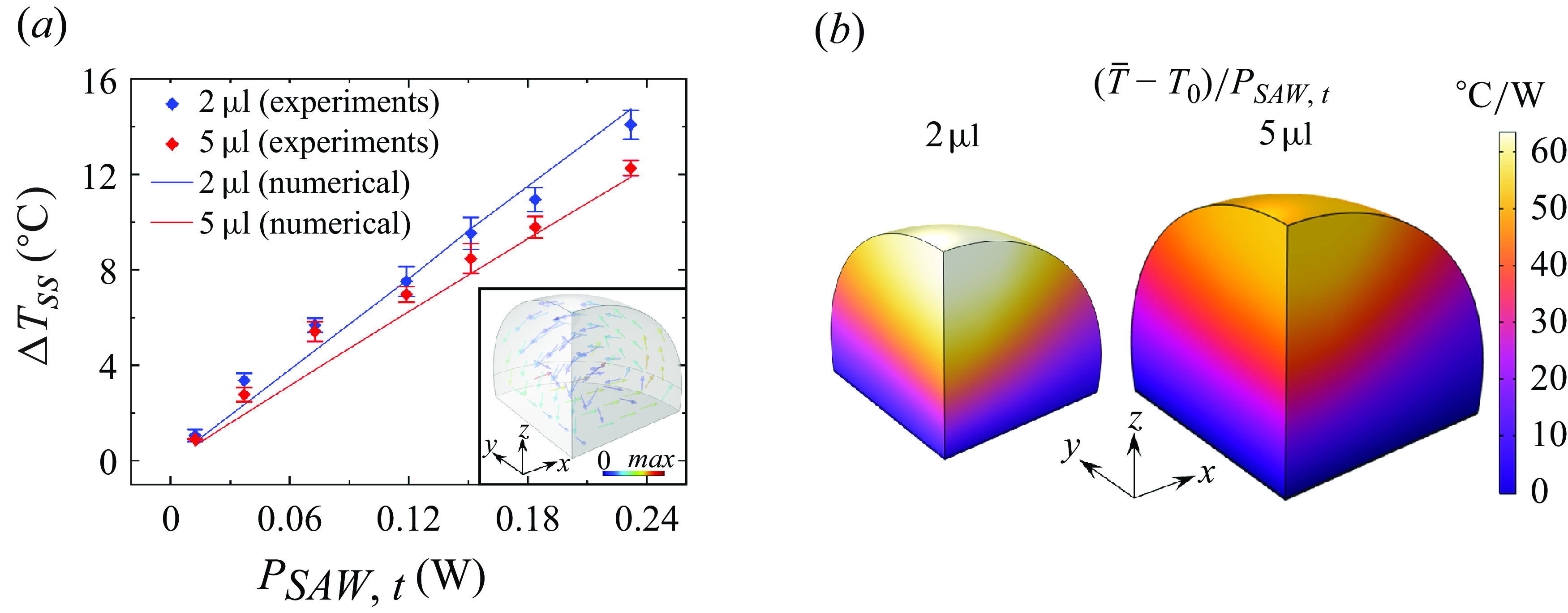
Figure 5. Acoustothermal temperature rise. (a) Dependence of steady acoustothermal temperature rise, $\Delta T_{{ss}}$
, on total acoustic power into the droplet,
$\Delta T_{{ss}}$
, on total acoustic power into the droplet, $P_{{SAW,t}}$
, for
$P_{{SAW,t}}$
, for $2 \, \unicode{x03BC} \text{l}$
(blue) and
$2 \, \unicode{x03BC} \text{l}$
(blue) and $5 \, \unicode{x03BC} \text{l}$
(red) droplets. The droplets are placed on a lithium-niobate-based SAW device and actuated by a
$5 \, \unicode{x03BC} \text{l}$
(red) droplets. The droplets are placed on a lithium-niobate-based SAW device and actuated by a $32.016 \, \text{MHz}$
standing SAW. The symbols and lines indicate experimental and numerical results, respectively. The inset shows the acoustic streaming velocity vectors inside the sessile droplet. The convective heat transport by the acoustic streaming is shown to reduce the droplet temperature rise by
$32.016 \, \text{MHz}$
standing SAW. The symbols and lines indicate experimental and numerical results, respectively. The inset shows the acoustic streaming velocity vectors inside the sessile droplet. The convective heat transport by the acoustic streaming is shown to reduce the droplet temperature rise by $2\,\%$
. Due to symmetry, only one quarter of the droplet system is shown. (b) Steady temperature distribution inside one quarter of 2 and
$2\,\%$
. Due to symmetry, only one quarter of the droplet system is shown. (b) Steady temperature distribution inside one quarter of 2 and $5 \, \unicode{x03BC} \text{l}$
droplets, estimated by numerical simulation. As
$5 \, \unicode{x03BC} \text{l}$
droplets, estimated by numerical simulation. As $(\bar {T} - T_0)$
shows linear dependence in the current operating SAW power window, the temperature distribution has been shown by scaling it with the total input SAW power.
$(\bar {T} - T_0)$
shows linear dependence in the current operating SAW power window, the temperature distribution has been shown by scaling it with the total input SAW power.

Figure 6. Effect of viscosity on acoustothermal temperature rise. (a) The dependence of the steady acoustothermal temperature rise, $\Delta T_{ss}$
, on total SAW power,
$\Delta T_{ss}$
, on total SAW power, $P_{\textit{SAW,t}}$
, for droplets of pure water (blue), 10 wt% glycerol (olive) and 20 wt% glycerol (red). The droplets have a constant volume of 5
$P_{\textit{SAW,t}}$
, for droplets of pure water (blue), 10 wt% glycerol (olive) and 20 wt% glycerol (red). The droplets have a constant volume of 5 $\unicode{x03BC}$
l and a contact angle of 100.63
$\unicode{x03BC}$
l and a contact angle of 100.63 $^\circ$
and are placed on a lithium-niobate-based SAW device actuated by a 32.016 MHz standing SAW. (b) The steady acoustothermal temperature rise,
$^\circ$
and are placed on a lithium-niobate-based SAW device actuated by a 32.016 MHz standing SAW. (b) The steady acoustothermal temperature rise, $\Delta T_{ss}$
, scaled by total SAW power,
$\Delta T_{ss}$
, scaled by total SAW power, $P_{{SAW,t}}$
, as a function of glycerol wt% (blue), alongside the corresponding variation in attenuation length,
$P_{{SAW,t}}$
, as a function of glycerol wt% (blue), alongside the corresponding variation in attenuation length, $L_{{w}}$
(red). (c) The variation of the maximum acoustic streaming velocity (
$L_{{w}}$
(red). (c) The variation of the maximum acoustic streaming velocity ( $U_{max }$
) inside droplets of pure water (blue), 10 wt% glycerol (olive) and 20 wt% glycerol (red) as a function of total SAW power,
$U_{max }$
) inside droplets of pure water (blue), 10 wt% glycerol (olive) and 20 wt% glycerol (red) as a function of total SAW power, $P_{\textit{SAW,t}}$
. The inset illustrates the dependence of the average acoustic streaming velocity (
$P_{\textit{SAW,t}}$
. The inset illustrates the dependence of the average acoustic streaming velocity ( $U_{{\textit{avg}}}$
) on total SAW power. (d) The variation of
$U_{{\textit{avg}}}$
) on total SAW power. (d) The variation of $U_{max }$
(red) and
$U_{max }$
(red) and $U_{{\textit{avg}}}$
(blue) with glycerol wt%. Since both
$U_{{\textit{avg}}}$
(blue) with glycerol wt%. Since both $U_{max }$
and
$U_{max }$
and $U_{{\textit{avg}}}$
exhibit linear dependence within the current SAW power range, they are scaled by
$U_{{\textit{avg}}}$
exhibit linear dependence within the current SAW power range, they are scaled by $P_{\textit{SAW},t}$
. The inset presents a log–log plot of
$P_{\textit{SAW},t}$
. The inset presents a log–log plot of $U_{max }^*$
and the kinematic viscosity (
$U_{max }^*$
and the kinematic viscosity ( $\nu$
), revealing the scaling relations
$\nu$
), revealing the scaling relations $U_{max }^* \propto \nu ^{-0.46}$
and
$U_{max }^* \propto \nu ^{-0.46}$
and $U_{{\textit{avg}}}^* \propto \nu ^{-0.64}$
. Throughout these graphs, symbols denote numerical results, dashed lines represent linear fits, and solid straight lines connect numerical data points to illustrate the overall trend.
$U_{{\textit{avg}}}^* \propto \nu ^{-0.64}$
. Throughout these graphs, symbols denote numerical results, dashed lines represent linear fits, and solid straight lines connect numerical data points to illustrate the overall trend.
5.4. Effect of fluid viscosity on acoustothermal phenomena
The influence of fluid viscosity on acoustothermal heating is of paramount significance, as viscous damping governs the conversion of acoustic energy into thermal energy. To elucidate this phenomenon, we conducted a numerical investigation of droplets composed of glycerol–water mixtures with glycerol weight percentages ( $W_{\textit{glyc}}$
) varying from 0 % (pure water) to 20 %, while maintaining a constant droplet volume of 5
$W_{\textit{glyc}}$
) varying from 0 % (pure water) to 20 %, while maintaining a constant droplet volume of 5 $\mathrm{\unicode{x03BC} l}$
and a contact angle of
$\mathrm{\unicode{x03BC} l}$
and a contact angle of $100.63^{\circ }$
. The pertinent thermophysical properties, including density, viscosity, thermal expansion coefficient, thermal conductivity and specific heat capacity were adopted from established literature sources (Perry Reference Perry1950; Cheng Reference Cheng2008; Delgado et al. Reference Delgado, Martínez, Fakhree and Jouyban2012) and are listed in the Supplementary Material. Figure 6
a illustrates the steady-state acoustothermal temperature rise,
$100.63^{\circ }$
. The pertinent thermophysical properties, including density, viscosity, thermal expansion coefficient, thermal conductivity and specific heat capacity were adopted from established literature sources (Perry Reference Perry1950; Cheng Reference Cheng2008; Delgado et al. Reference Delgado, Martínez, Fakhree and Jouyban2012) and are listed in the Supplementary Material. Figure 6
a illustrates the steady-state acoustothermal temperature rise, $\Delta T_{ss}$
, for sessile droplets as a function of input SAW power,
$\Delta T_{ss}$
, for sessile droplets as a function of input SAW power, $P_{{SAW,t}}$
, for
$P_{{SAW,t}}$
, for $W_{\textit{glyc}} = 0\,\%$
(pure water), 10 % and 20 %. Notably, the viscous influence in a 20 wt% glycerol–water mixture is nearly twofold that of pure water. Within the SAW power regime considered in the present study, the acoustothermal temperature rise exhibits a linear dependence on the total input SAW power across all cases. As the glycerol wt% increases, acoustic wave attenuation becomes more pronounced, substantially altering the internal acoustic field distribution within the droplet and, consequently, modulating acoustothermal effects. Given that
$W_{\textit{glyc}} = 0\,\%$
(pure water), 10 % and 20 %. Notably, the viscous influence in a 20 wt% glycerol–water mixture is nearly twofold that of pure water. Within the SAW power regime considered in the present study, the acoustothermal temperature rise exhibits a linear dependence on the total input SAW power across all cases. As the glycerol wt% increases, acoustic wave attenuation becomes more pronounced, substantially altering the internal acoustic field distribution within the droplet and, consequently, modulating acoustothermal effects. Given that $\Delta T_{ss} \propto P_{{SAW,t}}$
, we normalise
$\Delta T_{ss} \propto P_{{SAW,t}}$
, we normalise $\Delta T_{ss}$
by
$\Delta T_{ss}$
by $P_{{SAW,t}}$
, and figure 6
b shows the scaled acoustothermal temperature rise,
$P_{{SAW,t}}$
, and figure 6
b shows the scaled acoustothermal temperature rise, ${\Delta T_{ss}}/{P_{{SAW,t}}}$
, as a function of glycerol wt%, alongside the corresponding variation in attenuation length,
${\Delta T_{ss}}/{P_{{SAW,t}}}$
, as a function of glycerol wt%, alongside the corresponding variation in attenuation length, $L_w$
. The intricate relationship between shear and bulk viscosities, collectively represented by the term
$L_w$
. The intricate relationship between shear and bulk viscosities, collectively represented by the term $\mu (1+\beta)$
, dictates the acoustic attenuation length, expressed as
$\mu (1+\beta)$
, dictates the acoustic attenuation length, expressed as $L_w = {1}/{2\alpha }$
. With increasing glycerol %,
$L_w = {1}/{2\alpha }$
. With increasing glycerol %, $L_w$
decreases from 22.4 mm in pure water to 15.5 mm in 20 wt% glycerol, reflecting a enhanced attenuation of the acoustic wave within the droplet. This intensified wave attenuation facilitates a more efficient conversion of acoustic energy into heat. Evidently,
$L_w$
decreases from 22.4 mm in pure water to 15.5 mm in 20 wt% glycerol, reflecting a enhanced attenuation of the acoustic wave within the droplet. This intensified wave attenuation facilitates a more efficient conversion of acoustic energy into heat. Evidently, $\Delta T_{ss}$
by
$\Delta T_{ss}$
by $P_{{SAW,t}}$
exhibits an inverse correlation with
$P_{{SAW,t}}$
exhibits an inverse correlation with $L_w$
, as illustrated in figure 6(b). The degree of wave attenuation significantly impacts the number of internal wave reflections within the droplet, thereby altering the acoustic streaming patterns. To precisely explain this effect, we introduce a dimensionless ratio,
$L_w$
, as illustrated in figure 6(b). The degree of wave attenuation significantly impacts the number of internal wave reflections within the droplet, thereby altering the acoustic streaming patterns. To precisely explain this effect, we introduce a dimensionless ratio, $\Lambda = {R}/{L_w}$
, which characterises the relationship between the droplet radius and the attenuation length. With increasing glycerol wt%,
$\Lambda = {R}/{L_w}$
, which characterises the relationship between the droplet radius and the attenuation length. With increasing glycerol wt%, $\Lambda$
exhibits an increasing trend, indicative of a reduction in the number of internal wave reflections. Nevertheless, within the parameter space of the present study,
$\Lambda$
exhibits an increasing trend, indicative of a reduction in the number of internal wave reflections. Nevertheless, within the parameter space of the present study, $\Lambda \ll 1$
across all cases, thereby ensuring that the acoustic streaming pattern remains stable, forming caustics with a characteristic four-eddy flow structure, consistent with the observations of Riaud et al. (Reference Riaud, Baudoin, Bou Matar, Thomas and Brunet2017). Figure 6(c) further demonstrates that both the maximum (
$\Lambda \ll 1$
across all cases, thereby ensuring that the acoustic streaming pattern remains stable, forming caustics with a characteristic four-eddy flow structure, consistent with the observations of Riaud et al. (Reference Riaud, Baudoin, Bou Matar, Thomas and Brunet2017). Figure 6(c) further demonstrates that both the maximum ( $U_{max }$
) and average (
$U_{max }$
) and average ( $U_{\textit{avg}}$
) acoustic streaming velocities (see inset of figure 6
c) vary linearly with SAW power. To facilitate a comparative analysis, we scaled streaming velocities as
$U_{\textit{avg}}$
) acoustic streaming velocities (see inset of figure 6
c) vary linearly with SAW power. To facilitate a comparative analysis, we scaled streaming velocities as ${U_{max }}/{P_{{SAW}}}$
and
${U_{max }}/{P_{{SAW}}}$
and ${U_{\textit{avg}}}/{P_{{SAW}}}$
, and plot their variation with glycerol wt% in figure 6
d. A linear decline in both maximum and average streaming velocities is observed with increasing glycerol wt%, indicating an enhanced suppression of the streaming due to the increasing viscous effects. The inset of figure 6
d depicts the dependence of scaled streaming velocities with kinematic viscosity of the droplet,
${U_{\textit{avg}}}/{P_{{SAW}}}$
, and plot their variation with glycerol wt% in figure 6
d. A linear decline in both maximum and average streaming velocities is observed with increasing glycerol wt%, indicating an enhanced suppression of the streaming due to the increasing viscous effects. The inset of figure 6
d depicts the dependence of scaled streaming velocities with kinematic viscosity of the droplet, $\nu$
, revealing pronounced scaling relations as
$\nu$
, revealing pronounced scaling relations as ${U_{max }}/{P_{{SAW}}} \propto \nu ^{-0.46}$
and
${U_{max }}/{P_{{SAW}}} \propto \nu ^{-0.46}$
and ${U_{\textit{avg}}}/{P_{{SAW}}} \propto \nu ^{-0.64}$
. Although the present study focuses on a standing SAW-actuated droplet system, this finding closely aligns with the scaling relation
${U_{\textit{avg}}}/{P_{{SAW}}} \propto \nu ^{-0.64}$
. Although the present study focuses on a standing SAW-actuated droplet system, this finding closely aligns with the scaling relation $U_{{\textit{avg}}} \propto \nu ^{-3/4}$
reported by Riaud et al. (Reference Riaud, Baudoin, Bou Matar, Thomas and Brunet2017) for a travelling SAW-actuated droplet system. Furthermore, we examine the impact of streaming-induced convective heat transport, which progressively weakens as streaming intensity diminishes with increasing glycerol concentration. Specifically, in the case of pure water, convective transport contributes to
$U_{{\textit{avg}}} \propto \nu ^{-3/4}$
reported by Riaud et al. (Reference Riaud, Baudoin, Bou Matar, Thomas and Brunet2017) for a travelling SAW-actuated droplet system. Furthermore, we examine the impact of streaming-induced convective heat transport, which progressively weakens as streaming intensity diminishes with increasing glycerol concentration. Specifically, in the case of pure water, convective transport contributes to $\sim 2\,\%$
reduction in
$\sim 2\,\%$
reduction in $\Delta T_{ss}$
, whereas this effect is considerably attenuated to a mere
$\Delta T_{ss}$
, whereas this effect is considerably attenuated to a mere $\sim 0.6\,\%$
reduction for 20 wt% glycerol droplets, underscoring the diminished contribution of streaming-mediated convective transport in more viscous fluids.
$\sim 0.6\,\%$
reduction for 20 wt% glycerol droplets, underscoring the diminished contribution of streaming-mediated convective transport in more viscous fluids.
5.5. Acoustic vs electromagnetic heating: analogous theory
In this section, we establish an analogy between our currently developed acoustothermal theory and the principles of electromagnetic heat generation. In electromagnetic theory (Maxwell Reference Maxwell1873), the propagation of electromagnetic waves is characterised by both the electric field $\mathbf{E}$
and magnetic field
$\mathbf{E}$
and magnetic field $\mathbf{H}$
, where the Poynting vector
$\mathbf{H}$
, where the Poynting vector $\mathbf{\Pi _{\textit{EM}}} = \mathbf{E} \times \mathbf{H}$
depicts the electromagnetic energy flux. According to Poynting’s theorem (Poynting Reference Poynting1884), the generalised conservation of energy yields
$\mathbf{\Pi _{\textit{EM}}} = \mathbf{E} \times \mathbf{H}$
depicts the electromagnetic energy flux. According to Poynting’s theorem (Poynting Reference Poynting1884), the generalised conservation of energy yields
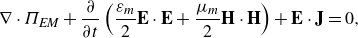 \begin{equation} \nabla \cdot \mathbf{\Pi _{\textit{EM}}} + \frac {\partial }{\partial t} \left ( \frac {\varepsilon _m}{2} \mathbf{E} \cdot \mathbf{E} + \frac {\mu _m}{2} \mathbf{H} \cdot \mathbf{H} \right) + \mathbf{E} \cdot \mathbf{J} = 0,\end{equation}
where $\varepsilon _m$
and
$\varepsilon _m$
and $\mu _m$
are the permittivity and the magnetic permeability of the medium. The conduction current density
$\mu _m$
are the permittivity and the magnetic permeability of the medium. The conduction current density $\mathbf{J}$
is related to the electric field as
$\mathbf{J}$
is related to the electric field as $\mathbf{J} = \sigma _m \mathbf{E}$
, where
$\mathbf{J} = \sigma _m \mathbf{E}$
, where $\sigma _m$
is the conductivity of the medium. The net electromagnetic power flow into a spatial region is given by
$\sigma _m$
is the conductivity of the medium. The net electromagnetic power flow into a spatial region is given by $-\nabla \cdot \mathbf{\Pi _{\textit{EM}}}$
, and it is balanced by the rate of change in the electric (
$-\nabla \cdot \mathbf{\Pi _{\textit{EM}}}$
, and it is balanced by the rate of change in the electric ( ${\varepsilon _m}/{2} \mathbf{E} \cdot \mathbf{E}$
) and magnetic (
${\varepsilon _m}/{2} \mathbf{E} \cdot \mathbf{E}$
) and magnetic ( ${\mu _m}/{2} \mathbf{H} \cdot \mathbf{H}$
) energy stored, along with the power dissipated (
${\mu _m}/{2} \mathbf{H} \cdot \mathbf{H}$
) energy stored, along with the power dissipated ( $\mathbf{E} \cdot \mathbf{J}$
), manifesting heat.
$\mathbf{E} \cdot \mathbf{J}$
), manifesting heat.
Analogous to electromagnetic theory, the Poynting vector in acoustic theory, which represents the acoustic energy flux, can be described as $\mathbf{\Pi _{\textit{ac}}} = \tilde {p} \, \tilde {\mathbf{v}}$
. Unlike electromagnetic waves, where power flow occurs in the direction perpendicular to both the electric and magnetic fields, the acoustic power flows coherently along the direction of the acoustic wave propagation. It is noteworthy that (5.1) constitutes the Poynting theorem analogous to that of electromagnetic theory. The electromagnetic heat source can fundamentally be expressed as
$\mathbf{\Pi _{\textit{ac}}} = \tilde {p} \, \tilde {\mathbf{v}}$
. Unlike electromagnetic waves, where power flow occurs in the direction perpendicular to both the electric and magnetic fields, the acoustic power flows coherently along the direction of the acoustic wave propagation. It is noteworthy that (5.1) constitutes the Poynting theorem analogous to that of electromagnetic theory. The electromagnetic heat source can fundamentally be expressed as $\langle q_{\textit{EM}} \rangle = -\langle \nabla \cdot \mathbf{\Pi _{\textit{EM}}} \rangle$
, similar to that of the acoustic theory developed in this study. The time-averaged value of
$\langle q_{\textit{EM}} \rangle = -\langle \nabla \cdot \mathbf{\Pi _{\textit{EM}}} \rangle$
, similar to that of the acoustic theory developed in this study. The time-averaged value of ${\partial }/{\partial t} ( {\varepsilon _m}/{2} \mathbf{E} \cdot \mathbf{E} + {\mu _m}/{2} \mathbf{H} \cdot \mathbf{H})$
is essentially zero, resulting in the electromagnetic source term as
${\partial }/{\partial t} ( {\varepsilon _m}/{2} \mathbf{E} \cdot \mathbf{E} + {\mu _m}/{2} \mathbf{H} \cdot \mathbf{H})$
is essentially zero, resulting in the electromagnetic source term as $\langle q_{\textit{EM}} \rangle = \sigma _m \langle \mathbf{E} \cdot \mathbf{E} \rangle.$
In the acoustic analogy, this is equivalent to the acoustothermal heat source given by (4.11).
$\langle q_{\textit{EM}} \rangle = \sigma _m \langle \mathbf{E} \cdot \mathbf{E} \rangle.$
In the acoustic analogy, this is equivalent to the acoustothermal heat source given by (4.11).
6. Conclusions
In conclusion, we extensively investigated the origin and underlying mechanism of acoustothermal effects in sessile water droplet systems actuated by standing SAWs using experimental, theoretical and numerical studies. We develop a novel theory to precisely calculate the acoustic fields and the mean dynamics, without employing a traditional perturbation approach. The limitation of existing theory in estimating the acoustothermal heat source is vividly discussed and the closed-form heat source expression provided in this study is extensively validated both theoretically and numerically. Furthermore, we have investigated the influence of viscosity on acoustothermal effects by numerically analysing the temperature distribution within sessile droplets composed of glycerol–water mixtures, thereby demonstrating the pivotal role of viscosity in modulating the acoustic field distribution and consequently shaping the acoustothermal profile of the droplet. An analogy with existing electromagnetic heating theory has been developed to delineate the mechanism and origin of the acoustothermal effects. Analogous to electromagnetic theory, the acoustic power flows along the propagation direction of the acoustic wave and the acoustothermal heat generation is characterised by the negative divergence of the acoustic Poynting vector. The dissipation of acoustic power is shown to be depended on the viscous damping factor, acoustic frequency and the kinetic energy density. We provided direct experimental evidence in quantifying and validating the acoustothermal dynamics in sessile droplet systems.
Supplementary materials
Supplementary materials are available at https://doi.org/10.1017/jfm.2025.10179.
Acknowledgements
We thank Y. Huang for the fabrication of the SAW device. We also thank Professor A. Riaud for the assistance in developing the Fourier-transform-based model for the acoustic field computations.
Funding
This work was funded by the National Science Foundation Grant No. CMI-2108795.
Declaration of interests
The authors report no conflict of interest.
Appendix A. Acoustothermal heat source in terms of viscous damping
The acoustothermal heat source can be expressed in terms of the divergence of the Poynting vector as expressed in (4.10). We can rewrite it as
 \begin{equation} \langle q_{\textit{ac}} \rangle = -\langle \tilde {p} \nabla \cdot \tilde {\mathbf{v}} + \nabla \tilde {p} \cdot \tilde {\mathbf{v}} \rangle.\end{equation}
Utilising (3.8a) and (4.2), we can express (A1) as
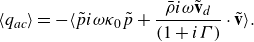 \begin{equation} \langle q_{\textit{ac}} \rangle = -\langle \tilde {p} i \omega \kappa _0 \tilde {p} + \frac {\bar {\rho} i \omega \tilde {\mathbf{v}}_d}{(1 + i \Gamma)} \cdot \tilde {\mathbf{v}} \rangle.\end{equation}
Replacing $i \omega (\tilde {\cdot })$
with
$i \omega (\tilde {\cdot })$
with ${\partial }/{\partial t} (\tilde {\cdot })$
, and utilising the fact
${\partial }/{\partial t} (\tilde {\cdot })$
, and utilising the fact $\Gamma \ll 1$
, we get
$\Gamma \ll 1$
, we get
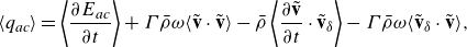 \begin{equation} \langle q_{\textit{ac}} \rangle = \left \langle \frac {\partial E_{\textit{ac}}}{\partial t} \right \rangle + \Gamma {\bar {\rho}} \omega \langle \tilde {\mathbf{v}} \cdot \tilde {\mathbf{v}} \rangle - {\bar {\rho}} \left \langle \frac {\partial \tilde {\mathbf{v}}}{\partial t} \cdot \tilde {\mathbf{v}}_{\delta } \right \rangle - \Gamma {\bar {\rho}} \omega \langle \tilde {\mathbf{v}}_{\delta } \cdot \tilde {\mathbf{v}} \rangle,\end{equation}
where $E_{\textit{ac}} = {1}/{2} \kappa _0 (\tilde {p} \tilde {p}) + {1}/{2} \bar{\rho} (\tilde {\mathbf{v}} \cdot \tilde {\mathbf{v}})$
is the acoustic energy density. Note here that the time-averaged value of the storage rate of acoustic energy density, i.e.
$E_{\textit{ac}} = {1}/{2} \kappa _0 (\tilde {p} \tilde {p}) + {1}/{2} \bar{\rho} (\tilde {\mathbf{v}} \cdot \tilde {\mathbf{v}})$
is the acoustic energy density. Note here that the time-averaged value of the storage rate of acoustic energy density, i.e. $\left \langle {\partial E_{\textit{ac}}}/{\partial t} \right \rangle$
, is zero. Since
$\left \langle {\partial E_{\textit{ac}}}/{\partial t} \right \rangle$
, is zero. Since $(\delta _{{vis}}, \delta _{{th}}) \ll \lambda$
, and
$(\delta _{{vis}}, \delta _{{th}}) \ll \lambda$
, and $\tilde {\mathbf{v}}_{\delta }$
only exists inside the boundary layer, the contributions of the last two terms are negligibly small, resulting in
$\tilde {\mathbf{v}}_{\delta }$
only exists inside the boundary layer, the contributions of the last two terms are negligibly small, resulting in
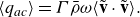 \begin{equation} \langle q_{\textit{ac}} \rangle = \Gamma {\bar {\rho}} \omega \langle \tilde {\mathbf{v}} \cdot \tilde {\mathbf{v}} \rangle.\end{equation}
Appendix B. Fourier-transform-based acoustic field computations
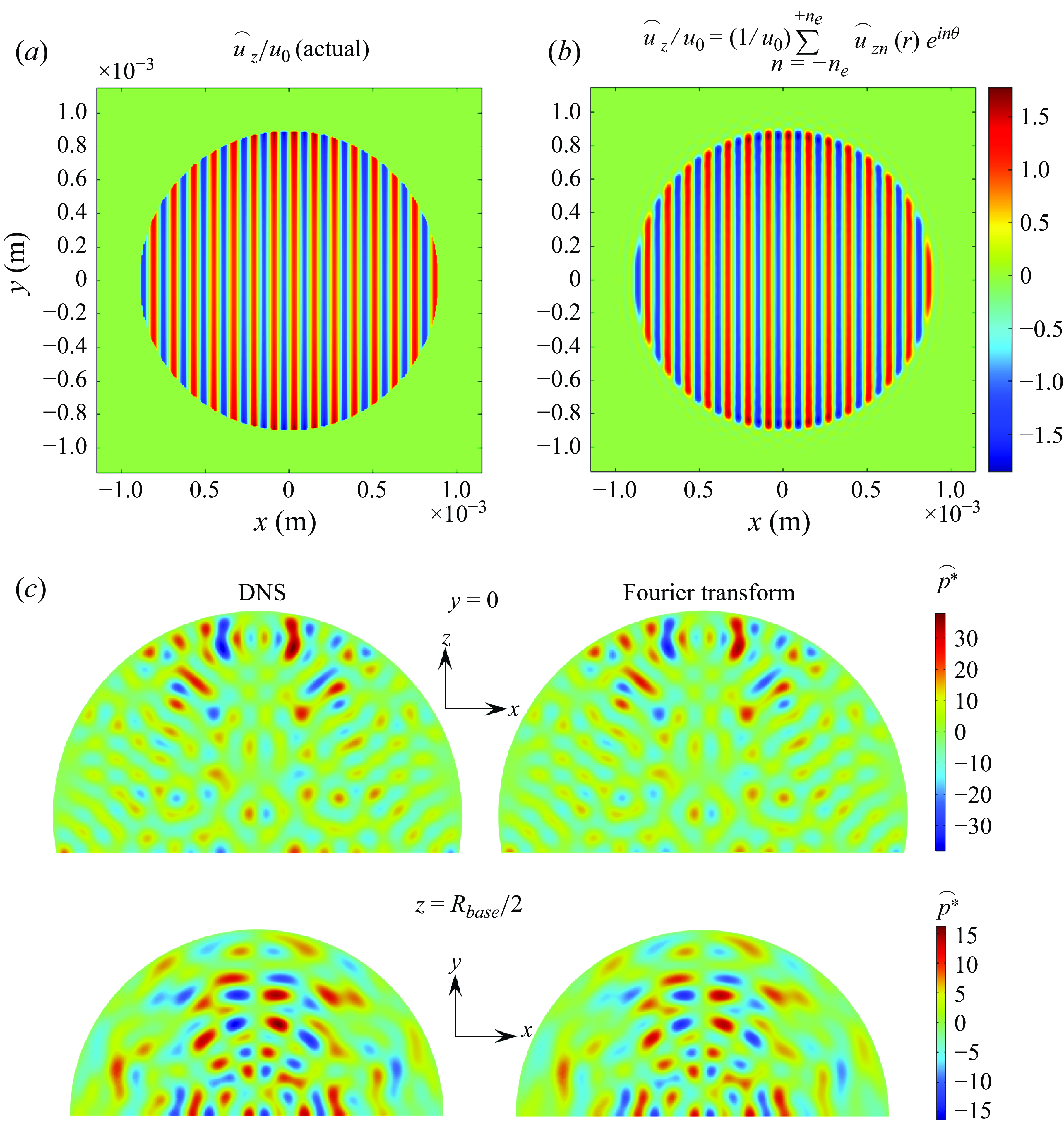
Figure 7. (a) The actual displacement field ${\tilde {u}_z}/{u_0}$
and (b) the displacement field obtained from the Fourier transform for a droplet base corresponding to a 2
${\tilde {u}_z}/{u_0}$
and (b) the displacement field obtained from the Fourier transform for a droplet base corresponding to a 2 $\unicode{x03BC}$
l sessile droplet actuated by a standing SAW of wavelength 120
$\unicode{x03BC}$
l sessile droplet actuated by a standing SAW of wavelength 120 $\unicode{x03BC}\rm m$
. (c) Acoustic pressure field obtained from direct numerical simulation and from Fourier transform for a 2
$\unicode{x03BC}\rm m$
. (c) Acoustic pressure field obtained from direct numerical simulation and from Fourier transform for a 2 $\unicode{x03BC}$
l sessile droplet actuated by standing SAW of wavelength 300
$\unicode{x03BC}$
l sessile droplet actuated by standing SAW of wavelength 300 $\unicode{x03BC}\rm m$
.
$\unicode{x03BC}\rm m$
.
Figure 7(a)–(b) shows the comparison of the actual standing SAW displacement field at the droplet base with the computed one using Fourier transform. The Fourier-transform-based displacement field has been computed using the formula
 \begin{equation} \frac {\tilde {u}_z}{u_0} = \frac {1}{u_0} \sum _{n=-n_e}^{n_e} \tilde {u}_{z,n}(r) e^{in\theta }, \end{equation}
where the value of $n_e$
is taken as 100. This value of
$n_e$
is taken as 100. This value of $n_e$
is adequate to resolve the SAW actuation, as evident from the figure. The results have been shown for the droplet base corresponding to 2
$n_e$
is adequate to resolve the SAW actuation, as evident from the figure. The results have been shown for the droplet base corresponding to 2 $\unicode{x03BC}$
l sessile droplets.
$\unicode{x03BC}$
l sessile droplets.
Figure 7(c) shows the distribution of the acoustic pressure field inside the 2 $\unicode{x03BC}$
l sessile droplet excited by standing SAW with a wavelength of 300
$\unicode{x03BC}$
l sessile droplet excited by standing SAW with a wavelength of 300 $\unicode{x03BC}\rm m$
. We compare direct numerical simulation (DNS) results with the results obtained using Fourier transform. Since it is extremely difficult to perform DNS for a 2
$\unicode{x03BC}\rm m$
. We compare direct numerical simulation (DNS) results with the results obtained using Fourier transform. Since it is extremely difficult to perform DNS for a 2 $\unicode{x03BC}$
l sessile droplet excited by 120
$\unicode{x03BC}$
l sessile droplet excited by 120 $\unicode{x03BC}\rm m$
standing SAW with modern computational facilities, we run DNS considering 300
$\unicode{x03BC}\rm m$
standing SAW with modern computational facilities, we run DNS considering 300 $\unicode{x03BC}\rm m$
standing SAW, and our Fourier transform results are in good agreement with the DNS results.
$\unicode{x03BC}\rm m$
standing SAW, and our Fourier transform results are in good agreement with the DNS results.
Appendix C. Acoustothermal heat source in terms of viscous dissipation
We can rewrite the acoustothermal heat source given by (4.9) as
 \begin{equation} \langle q_{\textit{ac}} \rangle = \langle \tilde {\mathbf{v}} \cdot (\nabla \cdot \tilde {\boldsymbol{\sigma }}) \rangle + \langle \nabla \tilde {\mathbf{v}}: \tilde {\boldsymbol{\sigma }} \rangle - \langle \tilde {p} \nabla \cdot \tilde {\mathbf{v}} \rangle - \langle \nabla \tilde {p} \cdot \tilde {\mathbf{v}} \rangle.\end{equation}
Using (3.8b
), $\tilde {\boldsymbol{\sigma }}$
can be expressed in terms of acoustic pressure and velocity fields, and (C1) can be simplified to
$\tilde {\boldsymbol{\sigma }}$
can be expressed in terms of acoustic pressure and velocity fields, and (C1) can be simplified to
 \begin{equation} \langle q_{\textit{ac}} \rangle = \langle \tilde {\mathbf{v}} \cdot i\omega \bar {\rho } \tilde {\mathbf{v}} \rangle + \langle \nabla \tilde {\mathbf{v}}: \tilde {\boldsymbol{\sigma }} \rangle - \langle \tilde {p} \nabla \cdot \tilde {\mathbf{v}} \rangle. \end{equation}
The expression can be further simplified by substituting from (3.8a ) as
 \begin{equation} \langle q_{\textit{ac}} \rangle = \langle \tilde {\mathbf{v}} \cdot i\omega \bar {\rho } \tilde {\mathbf{v}} \rangle + \langle \nabla \tilde {\mathbf{v}}: \tilde {\boldsymbol{\sigma }} \rangle + \langle \tilde {p} i\omega \kappa _0 \tilde {p} \rangle. \end{equation}
Replacing $i\omega (\tilde {\cdot })$
with
$i\omega (\tilde {\cdot })$
with $\partial _t (\tilde {\cdot })$
, we can rewrite (C3) as
$\partial _t (\tilde {\cdot })$
, we can rewrite (C3) as
 \begin{equation} \langle q_{\textit{ac}} \rangle = \left\langle \frac {\partial E_{\textit{ac}}}{\partial t} \right\rangle + \langle \nabla \tilde {\mathbf{v}}: \tilde {\boldsymbol{\sigma }} \rangle.\end{equation}


 Open access