


1. Introduction
In the domain of melting, a phenomenon known as close-contact melting (CCM) stands out. Unlike conventional convection-driven melting with expanding molten liquid spaces, CCM involves a distinct process where the surface of an unmelted solid and a heating element are pressed together under external force. This results in the formation of a thin molten film flow between the solid and heating surfaces, facilitating solid–liquid phase change heat transfer at a low-Reynolds-number flow of the liquid. Close-contact melting can be observed in two primary modes: heat source-driven (constant pressure) and unmelted solid-driven (gravity-driven) (Hu et al. Reference Hu, Li, Xu and Fan2022), depending on the external force applied to the object. The former mode refers to the scenario where the heated surface penetrates into an unmelted solid, which includes glacier drilling by heating (Schuller, Kowalski & Raback Reference Schuller, Kowalski and Raback2016), subtractive machining (Mayer & Moaveni Reference Mayer and Moaveni2008) and the ‘melt down’ of nuclear fuel (Emerman & Turcotte Reference Emerman and Turcotte1983). The latter mode can be observed readily in daily life, such as when ice, butter or chocolate melts on a heated substrate. Also, it is found in latent heat thermal energy storage (Kozak, Rozenfeld & Ziskind Reference Kozak, Rozenfeld and Ziskind2014) and thermal management systems (Fu et al. Reference Fu, Yan, Gurumukhi, Garimella, King and Miljkovic2022), where a considerable heat flux can be achieved easily. In the area of thermal energy storage, the melting rate is equivalent to the charging rate.
Given the widespread applications of CCM, it has been studied extensively for decades (Hu et al. Reference Hu, Li, Xu and Fan2022). These studies explore the effects of geometry (Moore & Bayazitoglu Reference Moore and Bayazitoglu1982; Sparrow & Geiger Reference Sparrow and Geiger1986; Dong et al. Reference Dong, Chen, Wang and Ebadian1991; Fomin, Wei & Chugunov Reference Fomin, Wei and Chugunov1995) and boundary conditions for heating (Moallemi & Viskanta Reference Moallemi and Viskanta1985; Saito et al. Reference Saito, Utaka, Akiyoshi and Katayama1985a
,Reference Saito, Utaka, Akiyoshi and Katayama
b
; Bejan Reference Bejan1992; Fomin, Saitoh & Chugunov Reference Fomin, Saitoh and Chugunov1997; Groulx & Lacroix Reference Groulx and Lacroix2007; Schueller & Kowalski Reference Schueller and Kowalski2017), with a primary focus on heat transfer characteristics. Recently, attention has shifted towards understanding the mechanisms of flow and heat transfer within the liquid film. Hu et al. measured the thickness variation of the thin film for the first time, confirming a magnitude of $O(10^2)$ $\unicode{x03BC}$
m (Hu et al. Reference Hu, Zhang, Zhang, Liu and Fan2019). Non-Newtonian features, including Bingham (Kozak et al. Reference Kozak, Zeng, Ghossein, Rabih, Khodadadi and Ziskind2019), power-law (Kozak Reference Kozak2023) and Carreau properties for the viscosity variations (Hu & Fan Reference Hu and Fan2023), as well as temperature-dependent properties (Cregan, Williams & Myers Reference Cregan, Williams and Myers2020), have been considered to study their impact on film thickness variation and flow behaviour. Strategies such as the use of permeable surfaces (Turkyilmazoglu Reference Turkyilmazoglu2019), slip surfaces (Aljaghtham, Premnath & Alsulami Reference Aljaghtham, Premnath and Alsulami2021; Kozak Reference Kozak2022) and pressure-enhanced conditions (Chen et al. Reference Chen, Liu, Gao and Wang2022; Fu et al. Reference Fu, Yan, Gurumukhi, Garimella, King and Miljkovic2022) have been proposed to accelerate melting.
$\unicode{x03BC}$
m (Hu et al. Reference Hu, Zhang, Zhang, Liu and Fan2019). Non-Newtonian features, including Bingham (Kozak et al. Reference Kozak, Zeng, Ghossein, Rabih, Khodadadi and Ziskind2019), power-law (Kozak Reference Kozak2023) and Carreau properties for the viscosity variations (Hu & Fan Reference Hu and Fan2023), as well as temperature-dependent properties (Cregan, Williams & Myers Reference Cregan, Williams and Myers2020), have been considered to study their impact on film thickness variation and flow behaviour. Strategies such as the use of permeable surfaces (Turkyilmazoglu Reference Turkyilmazoglu2019), slip surfaces (Aljaghtham, Premnath & Alsulami Reference Aljaghtham, Premnath and Alsulami2021; Kozak Reference Kozak2022) and pressure-enhanced conditions (Chen et al. Reference Chen, Liu, Gao and Wang2022; Fu et al. Reference Fu, Yan, Gurumukhi, Garimella, King and Miljkovic2022) have been proposed to accelerate melting.
In addition, hydrophobic or superhydrophobic surfaces with microscale-trapped air can provide an effective slip length, of the order of $O(10^2)$ $\unicode{x03BC}$
m, for liquid transport (Lee, Choi & Kim Reference Lee, Choi and Kim2008; Quéré Reference Quéré2008). This characteristic is considered a promising strategy for reducing liquid film thickness, thereby potentially enhancing heat transfer of CCM. Recently, Kozak theoretically studied postpatterned hydrophobic surfaces and showed that a temperature slip length
$\unicode{x03BC}$
m, for liquid transport (Lee, Choi & Kim Reference Lee, Choi and Kim2008; Quéré Reference Quéré2008). This characteristic is considered a promising strategy for reducing liquid film thickness, thereby potentially enhancing heat transfer of CCM. Recently, Kozak theoretically studied postpatterned hydrophobic surfaces and showed that a temperature slip length $\lambda ^{*}_{t}$
(the definition is given in § 2.2.1) greater than velocity slip length
$\lambda ^{*}_{t}$
(the definition is given in § 2.2.1) greater than velocity slip length $\lambda ^{*}$
(Kozak Reference Kozak2022) leads to a reduced heat transfer; the calculation utilised the formulae
$\lambda ^{*}$
(Kozak Reference Kozak2022) leads to a reduced heat transfer; the calculation utilised the formulae $ \lambda ^{*} / l^{*}=3 \sqrt {\pi /(1-\phi )}/16-3\ln (1+\sqrt {2})/(2 \pi )$
(Davis & Lauga Reference Davis and Lauga2010) and
$ \lambda ^{*} / l^{*}=3 \sqrt {\pi /(1-\phi )}/16-3\ln (1+\sqrt {2})/(2 \pi )$
(Davis & Lauga Reference Davis and Lauga2010) and $\lambda ^{*}=3\lambda ^{*}_t/4$
(Enright et al. Reference Enright, Hodes, Salamon and Muzychka2014), where
$\lambda ^{*}=3\lambda ^{*}_t/4$
(Enright et al. Reference Enright, Hodes, Salamon and Muzychka2014), where $^{*}$
represents dimensional quantities,
$^{*}$
represents dimensional quantities, $l^{*}$
is the period of a post pattern and
$l^{*}$
is the period of a post pattern and $\phi$
is the liquid–gas area fraction. Although this work established a framework for analysing velocity and temperature slip effects on CCM, the expressions for
$\phi$
is the liquid–gas area fraction. Although this work established a framework for analysing velocity and temperature slip effects on CCM, the expressions for $\lambda ^*$
rely on three assumptions: (i) shear flow in the liquid above the surface; (ii) a flat gas–liquid interface; (iii) perfect slip on the gas–liquid interface. Assumption (iii) is satisfied when
$\lambda ^*$
rely on three assumptions: (i) shear flow in the liquid above the surface; (ii) a flat gas–liquid interface; (iii) perfect slip on the gas–liquid interface. Assumption (iii) is satisfied when $ h_s^{*} {\mu _l^{*}}/{\mu _g^{*}} \gg l^{*}$
(Belyaev & Vinogradova Reference Belyaev and Vinogradova2010; Asmolov & Vinogradova Reference Asmolov and Vinogradova2012), where
$ h_s^{*} {\mu _l^{*}}/{\mu _g^{*}} \gg l^{*}$
(Belyaev & Vinogradova Reference Belyaev and Vinogradova2010; Asmolov & Vinogradova Reference Asmolov and Vinogradova2012), where $h_s^{*}$
,
$h_s^{*}$
, $ {\mu _l^{*}}$
and
$ {\mu _l^{*}}$
and $\mu _g^{*}$
denote microstructure height, liquid viscosity and gas viscosity, respectively. However, assumptions (i) and (ii) may not apply to CCM due to the features of Poiseuille flow and deformation of the meniscus, leading to a complicated effective slip. The assumption of a constant ratio
$\mu _g^{*}$
denote microstructure height, liquid viscosity and gas viscosity, respectively. However, assumptions (i) and (ii) may not apply to CCM due to the features of Poiseuille flow and deformation of the meniscus, leading to a complicated effective slip. The assumption of a constant ratio $\lambda _t^*/ \lambda ^*$
is valid for large aspect ratios
$\lambda _t^*/ \lambda ^*$
is valid for large aspect ratios $\Lambda \equiv h^*/l^*$
(Enright et al. Reference Enright, Hodes, Salamon and Muzychka2014), where
$\Lambda \equiv h^*/l^*$
(Enright et al. Reference Enright, Hodes, Salamon and Muzychka2014), where $h^*$
is the liquid film thickness. Furthermore, the slip lengths are governed by the geometrical patterns of the microstructure, which should be evaluated and compared.
$h^*$
is the liquid film thickness. Furthermore, the slip lengths are governed by the geometrical patterns of the microstructure, which should be evaluated and compared.
In the literature on slip, since the early works by Philip (Reference Philip1972a
,Reference Philip
b
), it has been shown that the velocity slip length $\lambda ^{*}$
is influenced by confinement effects (Lauga & Stone Reference Lauga and Stone2003; Sbragaglia & Prosperetti Reference Sbragaglia and Prosperetti2007; Teo & Khoo Reference Teo and Khoo2008; Feuillebois, Bazant & Vinogradova Reference Feuillebois, Bazant and Vinogradova2009; Schnitzer & Yariv Reference Schnitzer and Yariv2017; Landel et al. Reference Landel, Peaudecerf, Temprano-Coleto, Gibou, Goldstein and Luzzatto-Fegiz2020). The asymptotic limit of slip length for flow past transverse slip regions inside a tube (radius
$\lambda ^{*}$
is influenced by confinement effects (Lauga & Stone Reference Lauga and Stone2003; Sbragaglia & Prosperetti Reference Sbragaglia and Prosperetti2007; Teo & Khoo Reference Teo and Khoo2008; Feuillebois, Bazant & Vinogradova Reference Feuillebois, Bazant and Vinogradova2009; Schnitzer & Yariv Reference Schnitzer and Yariv2017; Landel et al. Reference Landel, Peaudecerf, Temprano-Coleto, Gibou, Goldstein and Luzzatto-Fegiz2020). The asymptotic limit of slip length for flow past transverse slip regions inside a tube (radius $R^*$
) has been determined (Lauga & Stone Reference Lauga and Stone2003), specifically
$R^*$
) has been determined (Lauga & Stone Reference Lauga and Stone2003), specifically $\lambda ^{*}_{\perp } / l^{*} \sim \ln (\sec (\phi \pi /2 ) )/(2\pi )$
when
$\lambda ^{*}_{\perp } / l^{*} \sim \ln (\sec (\phi \pi /2 ) )/(2\pi )$
when $l^{*}/R^{*} \ll 1$
, while
$l^{*}/R^{*} \ll 1$
, while $\lambda ^{*}_{ \perp }/R^{*} \sim \phi /(4-4\phi )$
when
$\lambda ^{*}_{ \perp }/R^{*} \sim \phi /(4-4\phi )$
when $l^{*}/R^{*} \gg 1$
; this result indicates that the velocity slip length can depend on the tube radius
$l^{*}/R^{*} \gg 1$
; this result indicates that the velocity slip length can depend on the tube radius $R^{*}$
instead of the pattern period
$R^{*}$
instead of the pattern period $l^{*}$
. Sbragaglia & Prosperetti (Reference Sbragaglia and Prosperetti2007) numerically obtained for longitudinal grooves a variation of velocity slip length
$l^{*}$
. Sbragaglia & Prosperetti (Reference Sbragaglia and Prosperetti2007) numerically obtained for longitudinal grooves a variation of velocity slip length $\lambda _{\parallel } = \lambda _{\parallel }^{*}/l^{*}$
for various aspect ratios
$\lambda _{\parallel } = \lambda _{\parallel }^{*}/l^{*}$
for various aspect ratios $\Lambda = h^{*} / l^{*}$
, where longitudinal means grooves oriented parallel to the flow, demonstrating that
$\Lambda = h^{*} / l^{*}$
, where longitudinal means grooves oriented parallel to the flow, demonstrating that $\lambda _{\parallel }$
remains constant when
$\lambda _{\parallel }$
remains constant when $\Lambda \geqslant 10$
, but shows a scaling law
$\Lambda \geqslant 10$
, but shows a scaling law $\lambda _{\parallel } \sim \Lambda$
when
$\lambda _{\parallel } \sim \Lambda$
when $\Lambda \lt 10$
. Similar confinement effects on the effective slip length can be found for either longitudinal or transverse grooves with symmetrical or asymmetrical boundary conditions (Teo & Khoo Reference Teo and Khoo2008; Schnitzer & Yariv Reference Schnitzer and Yariv2017) or on interfacial velocity at the liquid–gas interface (Landel et al. Reference Landel, Peaudecerf, Temprano-Coleto, Gibou, Goldstein and Luzzatto-Fegiz2020). An interesting fact related to confinement effects is that longitudinal grooves provide the largest slip lengths while transverse grooves yield the smallest ones in the limit of
$\Lambda \lt 10$
. Similar confinement effects on the effective slip length can be found for either longitudinal or transverse grooves with symmetrical or asymmetrical boundary conditions (Teo & Khoo Reference Teo and Khoo2008; Schnitzer & Yariv Reference Schnitzer and Yariv2017) or on interfacial velocity at the liquid–gas interface (Landel et al. Reference Landel, Peaudecerf, Temprano-Coleto, Gibou, Goldstein and Luzzatto-Fegiz2020). An interesting fact related to confinement effects is that longitudinal grooves provide the largest slip lengths while transverse grooves yield the smallest ones in the limit of $\Lambda \ll 1$
(Feuillebois et al. Reference Feuillebois, Bazant and Vinogradova2009). This contrasts with predictions for
$\Lambda \ll 1$
(Feuillebois et al. Reference Feuillebois, Bazant and Vinogradova2009). This contrasts with predictions for $\Lambda \gg 1$
, where arrays of posts have a larger slip length than grooves. Given the special feature of CCM that film thickness
$\Lambda \gg 1$
, where arrays of posts have a larger slip length than grooves. Given the special feature of CCM that film thickness $h^{*}$
(also the channel height) is variable and sensitive to conditions, we can consider the examples from Kozak (Reference Kozak2022), where
$h^{*}$
(also the channel height) is variable and sensitive to conditions, we can consider the examples from Kozak (Reference Kozak2022), where $l^{*} \sim 50 \ \unicode{x03BC}$
m and
$l^{*} \sim 50 \ \unicode{x03BC}$
m and $h^{*} \sim 50 \ \unicode{x03BC}$
m (
$h^{*} \sim 50 \ \unicode{x03BC}$
m ( $\phi =0.99$
), as well as
$\phi =0.99$
), as well as $l^{*} \sim 16 \ \unicode{x03BC}$
m and
$l^{*} \sim 16 \ \unicode{x03BC}$
m and $h^{*} \sim 80 \ \unicode{x03BC}$
m (
$h^{*} \sim 80 \ \unicode{x03BC}$
m ( $\phi =0.84$
). In this case, confinement effects may be non-negligible due to
$\phi =0.84$
). In this case, confinement effects may be non-negligible due to $1 \leqslant \Lambda \leqslant 5$
.
$1 \leqslant \Lambda \leqslant 5$
.
At the same time, another issue arises concerning the curved gas–liquid interface due to the wide variation of pressure exerted on the liquid film in CCM. It has been demonstrated that meniscus protrusion into cavities will either increase or decrease the slip length $\lambda ^{*}$
depending on the aspect ratio
$\lambda ^{*}$
depending on the aspect ratio $\Lambda$
(Sbragaglia & Prosperetti Reference Sbragaglia and Prosperetti2007; Teo & Khoo Reference Teo and Khoo2010; Crowdy Reference Crowdy2016; Game et al. Reference Game, Hodes, Keaveny and Papageorgiou2017; Kirk, Hodes & Papageorgiou Reference Kirk, Hodes and Papageorgiou2017). When
$\Lambda$
(Sbragaglia & Prosperetti Reference Sbragaglia and Prosperetti2007; Teo & Khoo Reference Teo and Khoo2010; Crowdy Reference Crowdy2016; Game et al. Reference Game, Hodes, Keaveny and Papageorgiou2017; Kirk, Hodes & Papageorgiou Reference Kirk, Hodes and Papageorgiou2017). When $\Lambda \gg 1$
, both slip lengths
$\Lambda \gg 1$
, both slip lengths $\lambda ^{*}_{\perp }$
and
$\lambda ^{*}_{\perp }$
and $\lambda ^{*}_{\parallel }$
decrease along with a larger meniscus angle
$\lambda ^{*}_{\parallel }$
decrease along with a larger meniscus angle $\theta$
that protrudes into grooves (Teo & Khoo Reference Teo and Khoo2010). However, for
$\theta$
that protrudes into grooves (Teo & Khoo Reference Teo and Khoo2010). However, for $ \Lambda \ll 1$
, the slip length
$ \Lambda \ll 1$
, the slip length $\lambda ^{*}$
can be increased by a meniscus for symmetrical boundaries (Sbragaglia & Prosperetti Reference Sbragaglia and Prosperetti2007; Kirk et al. Reference Kirk, Hodes and Papageorgiou2017). Besides the velocity slip length
$\lambda ^{*}$
can be increased by a meniscus for symmetrical boundaries (Sbragaglia & Prosperetti Reference Sbragaglia and Prosperetti2007; Kirk et al. Reference Kirk, Hodes and Papageorgiou2017). Besides the velocity slip length $\lambda ^{*}$
, confinement and meniscus effects also play an important role in the temperature slip length
$\lambda ^{*}$
, confinement and meniscus effects also play an important role in the temperature slip length $\lambda ^{*}_{t}$
(Enright et al. Reference Enright, Hodes, Salamon and Muzychka2014; Kirk et al. Reference Kirk, Hodes and Papageorgiou2017; Hodes et al. Reference Hodes, Kane, Bazant and Kirk2023; Tomlinson et al. Reference Tomlinson, Mayer, Kirk, Hodes and Papageorgiou2024). The primary conclusions drawn are that the confinement effect results in a larger temperature slip length, while meniscus influences tend to reduce it. However, for CCM studies, the latter has not been considered (Kozak Reference Kozak2022).
$\lambda ^{*}_{t}$
(Enright et al. Reference Enright, Hodes, Salamon and Muzychka2014; Kirk et al. Reference Kirk, Hodes and Papageorgiou2017; Hodes et al. Reference Hodes, Kane, Bazant and Kirk2023; Tomlinson et al. Reference Tomlinson, Mayer, Kirk, Hodes and Papageorgiou2024). The primary conclusions drawn are that the confinement effect results in a larger temperature slip length, while meniscus influences tend to reduce it. However, for CCM studies, the latter has not been considered (Kozak Reference Kozak2022).
1.1. Scope and structure of this work
Since constant-pressure and gravity-driven CCM are characterised by constant and growing liquid film thicknesses, respectively, as well as also corresponding to two different application scenarios, melt drilling and thermal energy storage, respectively, we focus on parallel-groove textured surfaces as a promising candidate for both modes of CCM, owing to the theoretical limit of a significant slip length for a given gas–liquid contact ratio (Feuillebois et al. Reference Feuillebois, Bazant and Vinogradova2009). Furthermore, by incorporating double re-entrant structures, these surfaces can readily maintain the Cassie state for a wide range of liquids (Liu & Kim Reference Liu and Kim2014; Wilke et al. Reference Wilke, Lu, Song and Wang2022). In § 2, we introduce the theoretical framework for CCM, considering the influences of the velocity slip length $\lambda$
and the temperature slip length
$\lambda$
and the temperature slip length $\lambda _t$
(noting that quantities without a
$\lambda _t$
(noting that quantities without a $^*$
are dimensionless), where the subscript
$^*$
are dimensionless), where the subscript $\parallel$
represents longitudinal grooves; also,
$\parallel$
represents longitudinal grooves; also, $f$
and
$f$
and $c$
denote flat interfaces and curved interfaces (menisci), respectively. Specifically, dimensional analysis of the problem is presented in § 2.1, followed by the derivation of the effective thermal slip length
$c$
denote flat interfaces and curved interfaces (menisci), respectively. Specifically, dimensional analysis of the problem is presented in § 2.1, followed by the derivation of the effective thermal slip length $\lambda _{t,f}$
and
$\lambda _{t,f}$
and $\lambda _{t,c}$
, corresponding to a flat gas–liquid interface (§ 2.2.1) and a curved surface (§ 2.2.2), respectively. The effective velocity slip lengths
$\lambda _{t,c}$
, corresponding to a flat gas–liquid interface (§ 2.2.1) and a curved surface (§ 2.2.2), respectively. The effective velocity slip lengths $\lambda _{\parallel, f}$
and
$\lambda _{\parallel, f}$
and $\lambda _{\parallel, c}$
are derived for flat (§ 2.3.1) and the curved (§ 2.3.2) liquid–gas interface, respectively. Slip lengths for all cases are solved by the standard dual-series method, whose details are introduced in the appendices. Based on the obtained effective slip lengths, a generalised one-dimensional description is developed for both constant-pressure and gravity-driven CCM in § 2.4.
$\lambda _{\parallel, c}$
are derived for flat (§ 2.3.1) and the curved (§ 2.3.2) liquid–gas interface, respectively. Slip lengths for all cases are solved by the standard dual-series method, whose details are introduced in the appendices. Based on the obtained effective slip lengths, a generalised one-dimensional description is developed for both constant-pressure and gravity-driven CCM in § 2.4.
In § 3.1, we discuss the influences of the dimensionless film height $\Lambda$
on the slip lengths for the flat (§ 3.1.1) and curved (§ 3.1.2) gas–liquid interfaces. Asymptotic solutions of
$\Lambda$
on the slip lengths for the flat (§ 3.1.1) and curved (§ 3.1.2) gas–liquid interfaces. Asymptotic solutions of $\lambda$
and
$\lambda$
and $\lambda _t$
for
$\lambda _t$
for $\Lambda \gg 1$
and
$\Lambda \gg 1$
and $\Lambda \ll 1$
are summarised in table 1. In addition, a modified asymptotic solution for
$\Lambda \ll 1$
are summarised in table 1. In addition, a modified asymptotic solution for $\lambda _{\parallel, c}$
is proposed for a wide range of
$\lambda _{\parallel, c}$
is proposed for a wide range of $\Lambda \gtrsim 0.2$
. We then discuss the slip effects on constant-pressure CCM in § 3.2, revealing the critical conditions of
$\Lambda \gtrsim 0.2$
. We then discuss the slip effects on constant-pressure CCM in § 3.2, revealing the critical conditions of $\Lambda$
and
$\Lambda$
and $\phi$
to achieve a faster melting rate. On the other hand, we analyse gravity-driven CCM in § 3.3, under limiting conditions derived from the dimensionless periodic length
$\phi$
to achieve a faster melting rate. On the other hand, we analyse gravity-driven CCM in § 3.3, under limiting conditions derived from the dimensionless periodic length $l$
, and construct a
$l$
, and construct a $l$
-
$l$
- $\phi$
phase diagram to illustrate the influences of slip.
$\phi$
phase diagram to illustrate the influences of slip.
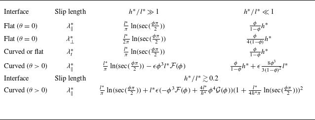
Table 1. Dimensional asymptotic formula of velocity ( $\lambda _{\parallel }^{*}$
or
$\lambda _{\parallel }^{*}$
or $\lambda _{\perp }^{*}$
) and thermal (
$\lambda _{\perp }^{*}$
) and thermal ( $\lambda _{t}^{*}$
) slip lengths for various confinement and meniscus effects.
$\lambda _{t}^{*}$
) slip lengths for various confinement and meniscus effects.
2. Physical model and theoretical framework
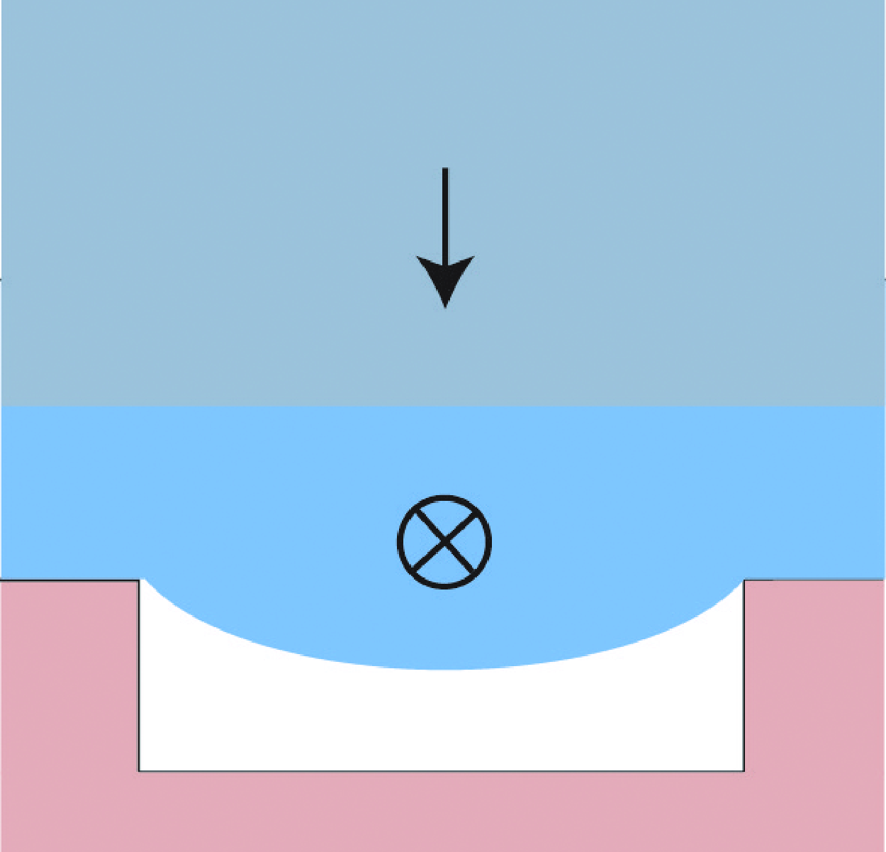
A typical CCM process on a microtextured hydrophobic surface is sketched in figure 1(a). Here and in the following, the notation $^{*}$
represents a dimensional quantity. A cuboid-shaped solid phase change material (PCM) with length
$^{*}$
represents a dimensional quantity. A cuboid-shaped solid phase change material (PCM) with length $L^{*}$
, width
$L^{*}$
, width $W^{*}$
and initial height
$W^{*}$
and initial height $H_{0}^{*}$
is heated from below by a textured (microgrooved) surface maintained at wall temperature
$H_{0}^{*}$
is heated from below by a textured (microgrooved) surface maintained at wall temperature $T_{w}^{*}$
and characterised by a periodic length
$T_{w}^{*}$
and characterised by a periodic length $l^{*}$
. The solid PCM, initially at its melting point
$l^{*}$
. The solid PCM, initially at its melting point $T_{m}^{*}\lt T_{w}^{*}$
, will continuously melt from the bottom under a certain pressure, which could be either a specific constant value
$T_{m}^{*}\lt T_{w}^{*}$
, will continuously melt from the bottom under a certain pressure, which could be either a specific constant value $\mathcal{P}^{*}$
or the self-weight pressure of the PCM,
$\mathcal{P}^{*}$
or the self-weight pressure of the PCM, $\rho _s^{*} g^{*} (H^{*}-h^{*})$
, depending on the mode of CCM. Given the microgrooved structure (periodic length
$\rho _s^{*} g^{*} (H^{*}-h^{*})$
, depending on the mode of CCM. Given the microgrooved structure (periodic length $l^*$
and gas fraction
$l^*$
and gas fraction $\phi$
), the mixed interface, composed of solid–liquid and gas–liquid contacts, when approximated with a one-dimensional description, introduces effective coefficients of temperature slip
$\phi$
), the mixed interface, composed of solid–liquid and gas–liquid contacts, when approximated with a one-dimensional description, introduces effective coefficients of temperature slip $\lambda _{t}^{*}$
and velocity slip
$\lambda _{t}^{*}$
and velocity slip $\lambda ^{*}$
, which are described below and significantly affect the fluid flow and heat transfer in the CCM process.
$\lambda ^{*}$
, which are described below and significantly affect the fluid flow and heat transfer in the CCM process.
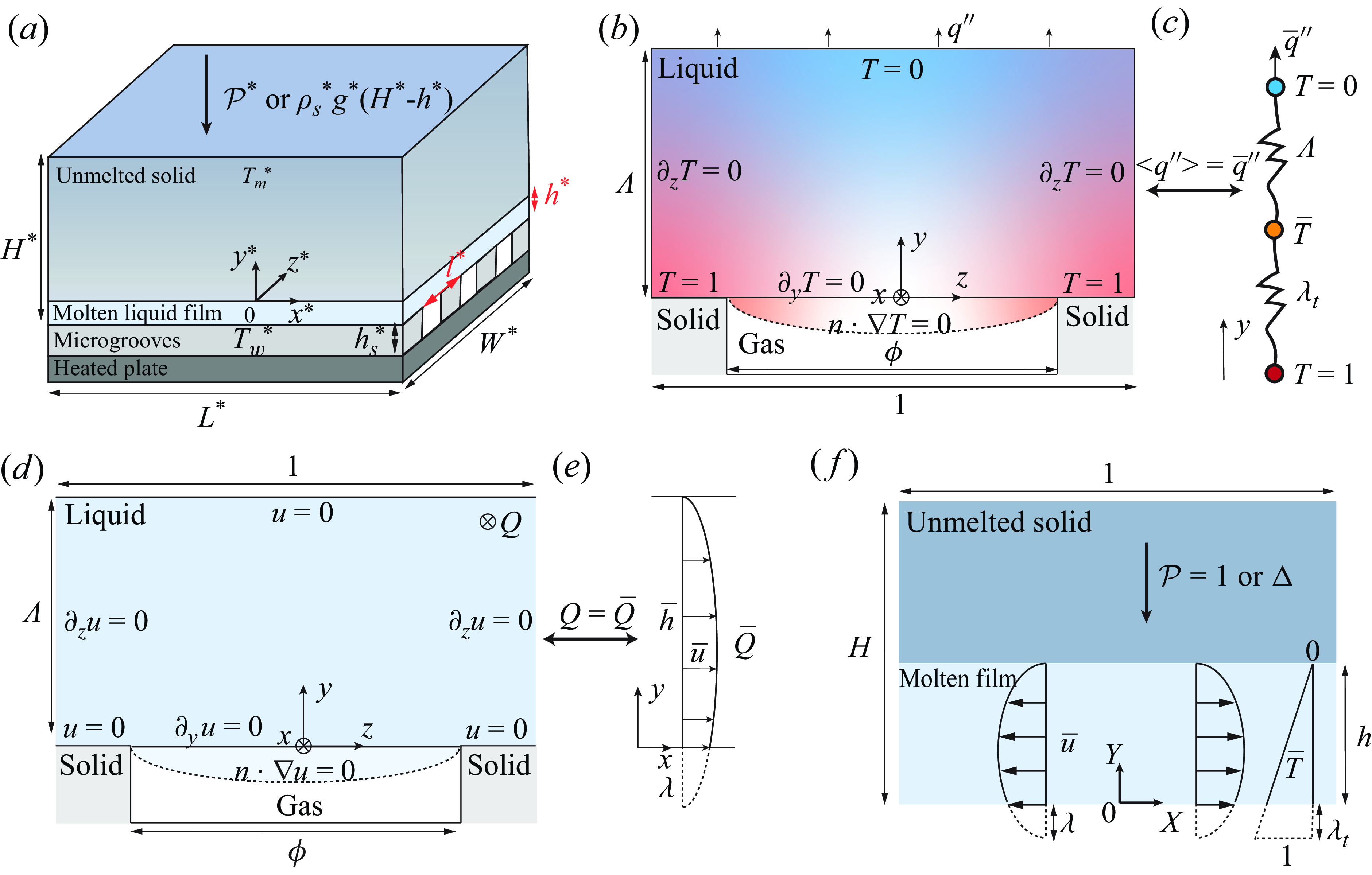
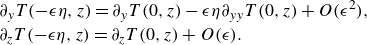
Figure 1. (a) Close-contact melting of a cuboid-shaped unmelted solid with initial height $H_{0}^{*}$
, length
$H_{0}^{*}$
, length $L^{*}$
and width
$L^{*}$
and width $W^{*}$
pressed downwards by constant pressure
$W^{*}$
pressed downwards by constant pressure $\mathcal{P}^{*}$
or self-weight
$\mathcal{P}^{*}$
or self-weight $\rho _s^*g^*(H^*-h^*)$
on a heated microgrooved hydrophobic surface with characteristic periodic length
$\rho _s^*g^*(H^*-h^*)$
on a heated microgrooved hydrophobic surface with characteristic periodic length $l^{*}$
, where
$l^{*}$
, where $h^*$
is the liquid film thickness; quantities with
$h^*$
is the liquid film thickness; quantities with $^{*}$
are dimensional. Schematic diagrams of boundary conditions for (b) two-dimensional descriptions, or (c) a one-dimensional description, for the temperature distribution and temperature slip length
$^{*}$
are dimensional. Schematic diagrams of boundary conditions for (b) two-dimensional descriptions, or (c) a one-dimensional description, for the temperature distribution and temperature slip length $\lambda _{t}$
; similarly, (d)–(e) characterise the velocity boundary conditions and velocity slip length
$\lambda _{t}$
; similarly, (d)–(e) characterise the velocity boundary conditions and velocity slip length $\lambda$
on the longitudinal grooves. It is noted that length is scaled by
$\lambda$
on the longitudinal grooves. It is noted that length is scaled by $l^{*}$
for convenience. (f) The dimensionless schematic diagram (
$l^{*}$
for convenience. (f) The dimensionless schematic diagram ( $L^* \ll W^*$
) by scaling as
$L^* \ll W^*$
) by scaling as $X = x^*/L^*$
,
$X = x^*/L^*$
, $Y = y^*/h_0^*$
and
$Y = y^*/h_0^*$
and $T = (T^*-T_m^*)/(T_w^*-T_m^*)$
, showing the remaining solid height
$T = (T^*-T_m^*)/(T_w^*-T_m^*)$
, showing the remaining solid height $H$
and film thickness
$H$
and film thickness $h$
is influenced by the effective velocity slip length
$h$
is influenced by the effective velocity slip length $\lambda$
and temperature slip length
$\lambda$
and temperature slip length $\lambda _{t}$
.
$\lambda _{t}$
.
2.1. Scaling analysis and non-dimensionalization
Typically, a thin melted film of liquid separates the substrate from the solid PCM. Hence, a lubrication-style analysis is suggested. The relevant physical parameters are the gravitational acceleration $g^{*}$
, viscosity
$g^{*}$
, viscosity $\mu ^{*}$
, solid density
$\mu ^{*}$
, solid density $\rho _s^{*}$
, liquid density
$\rho _s^{*}$
, liquid density $\rho _l^{*}$
, liquid specific heat capacity
$\rho _l^{*}$
, liquid specific heat capacity $c_{p,l}^{*}$
, thermal conductivity of liquid
$c_{p,l}^{*}$
, thermal conductivity of liquid $k_l^{*}$
and latent heat of fusion
$k_l^{*}$
and latent heat of fusion $\mathcal{H}^*$
. By scaling pressure and stresses with
$\mathcal{H}^*$
. By scaling pressure and stresses with $p_c^* = \rho _s^*g^*(H_0^*-h_0^*)$
for the gravity-driven mode or
$p_c^* = \rho _s^*g^*(H_0^*-h_0^*)$
for the gravity-driven mode or $p_c^* = \mathcal{P}^*$
for the constant-pressure mode, velocity with
$p_c^* = \mathcal{P}^*$
for the constant-pressure mode, velocity with $u_c^* = {h_0^*}^2p_c^*/(\mu ^*L^*)$
, time with
$u_c^* = {h_0^*}^2p_c^*/(\mu ^*L^*)$
, time with $t_c^* = L^*/u_c^*$
and temperature with
$t_c^* = L^*/u_c^*$
and temperature with $T_w^{*}-T_m^{*}$
, we can define dimensionless variables as
$T_w^{*}-T_m^{*}$
, we can define dimensionless variables as
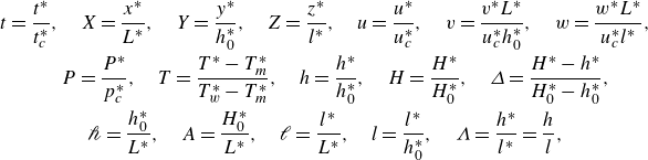 \begin{equation} \begin{gathered} t =\frac {t^*}{t_c^*}, \quad X=\frac {x^*}{L^*}, \quad Y=\frac {y^*}{h_0^*}, \quad Z=\frac {z^*}{l^*}, \quad u = \frac {u^*}{u_c^*}, \quad v = \frac {v^*L^*}{u_c^*h_0^*}, \quad w = \frac {w^*L^*}{u_c^*l^*},\\ \quad P = \frac {P^*}{p_c^*}, \quad T=\frac {T^*-T_m^*}{T_w^*-T_m^*},\quad h = \frac {h^*}{h_0^*}, \quad H =\frac {H^*}{H_0^*}, \quad \varDelta = \frac {H^*-h^*}{H_0^*-h_0^*}, \\ \mathscr{h} = \frac {h_0^*}{L^*}, \quad A = \frac {H_0^*}{L^*}, \quad \mathscr{l}=\frac {l^*}{L^*}, \quad l =\frac {l^*}{h_0^*},\quad \Lambda =\frac {h^*}{l^*}=\frac {h}{l}, \end{gathered} \end{equation}
where $h_0^*$
is the initial film thickness identified below as (2.51) in § 2.4. The aspect ratio
$h_0^*$
is the initial film thickness identified below as (2.51) in § 2.4. The aspect ratio $\Lambda$
is a key parameter related to the confinement effect in the following discussion. Hence, the dimensionless variables are denoted as the velocity vector
$\Lambda$
is a key parameter related to the confinement effect in the following discussion. Hence, the dimensionless variables are denoted as the velocity vector $\boldsymbol{V}\equiv u\boldsymbol{e}_X+v\boldsymbol{e}_Y+w\boldsymbol{e}_Z$
, temperature
$\boldsymbol{V}\equiv u\boldsymbol{e}_X+v\boldsymbol{e}_Y+w\boldsymbol{e}_Z$
, temperature $T$
, pressure
$T$
, pressure $P$
, spatial gradient operator
$P$
, spatial gradient operator $\boldsymbol{\nabla }\equiv \boldsymbol{e}_X\partial _X+\boldsymbol{e}_Y\partial _Y +\boldsymbol{e}_Z\partial _Z$
and
$\boldsymbol{\nabla }\equiv \boldsymbol{e}_X\partial _X+\boldsymbol{e}_Y\partial _Y +\boldsymbol{e}_Z\partial _Z$
and $\partial _t$
is the time derivative. The Reynolds number
$\partial _t$
is the time derivative. The Reynolds number $\textrm{Re}$
, Péclet number
$\textrm{Re}$
, Péclet number $\textrm{Pe}$
, Prandtl number
$\textrm{Pe}$
, Prandtl number $\textrm{Pr}$
, Eckert number
$\textrm{Pr}$
, Eckert number $\textrm{Ec}$
, Stefan number
$\textrm{Ec}$
, Stefan number $\textrm{St}$
, density ratio
$\textrm{St}$
, density ratio $\rho$
and hydrostatic pressure ratio
$\rho$
and hydrostatic pressure ratio $p_h$
are, respectively, defined as
$p_h$
are, respectively, defined as
 \begin{align}&\qquad\qquad\textrm{Re} \equiv \frac {\rho _l^*L^*u_c^*}{\mu ^*}, \quad \textrm{Pe} \equiv \frac {u_c^*L^*\rho _l^*c_{p,l}^*}{k_l^*}, \quad \textrm{Pr} \equiv \frac {\mu ^{*} c_{p,l}^{*}}{k_l^{*}}, \end{align}
 \begin{align}&\textrm{Ec} \equiv \frac {{u_c^*}^2}{ c_{p,l}^{*} \left (T_w^{*}-T_m^{*}\right )}, \quad \textrm{St} \equiv \frac {c_{p,l}^{*} \left (T_w^{*}-T_m^{*}\right )}{\mathcal{H}^*}, \quad \rho \equiv \frac {\rho _s^{*}}{\rho _l^{*}}, \quad p_h = \frac {\rho _l^*g^*h_0^*}{p_c^*}. \end{align}
In this case, the equations of continuity, momentum (in the $X$
,
$X$
, $Y$
-and
$Y$
-and $Z$
directions), and energy, including the dissipation of mechanical to thermal energy in the bulk liquid and an energy balance at the melting front, are, respectively,
$Z$
directions), and energy, including the dissipation of mechanical to thermal energy in the bulk liquid and an energy balance at the melting front, are, respectively,
 \begin{align}&\qquad\qquad\qquad\qquad\qquad\qquad\qquad \boldsymbol{\nabla } \cdot \boldsymbol{V}=0, \end{align}
 \begin{align}&\qquad\qquad \textrm{Re}\mathscr{h}^2\partial _t u + \textrm{Re}\mathscr{h}^2 ({\boldsymbol{V}} \cdot \boldsymbol{\nabla }) {u} = -\partial _X P + \mathscr{h}^2 \partial _X^2 u + \partial _Y^2 u + l^{-2} \partial _Z^2 u, \end{align}
 \begin{align}& {}\qquad\textrm{Re}\mathscr{h}^4\partial _t v + \textrm{Re}\mathscr{h}^4 ({\boldsymbol{V}} \cdot \boldsymbol{\nabla }) v = -\partial _Y P + \mathscr{h}^4 \partial _X^2 v + \mathscr{h}^2 \partial _Y^2 v + l^{-2} \mathscr{h}^2 \partial _Z^2 v + p_h, \end{align}
 \begin{align}& {}\qquad\,\,\,\textrm{Re}\mathscr{h}^2\mathscr{l}^2 \partial _t w + \textrm{Re}\mathscr{h}^2 \mathscr{l}^2 ({\boldsymbol{V}} \cdot \boldsymbol{\nabla }) w = -\partial _Z P + \mathscr{h}^2 \mathscr{l}^2 \partial _X^2 w + \mathscr{l}^2 \partial _Y^2 w + \mathscr{h}^2 \partial _Z^2 w, \end{align}
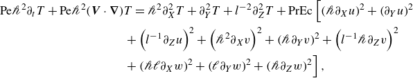 \begin{align}& \textrm{Pe}\mathscr{h}^2\partial _t T + \textrm{Pe}\mathscr{h}^2 ({\boldsymbol{V}} \cdot \boldsymbol{\nabla }) {T} = \mathscr{h}^2 \partial _X^2 T + \partial _Y^2 T + l^{-2} \partial _Z^2 T + \textrm{PrEc} \left [ \left ( \mathscr{h} \partial _X u \right )^2 + \left ( \partial _Y u \right )^2 \right . \nonumber\\ &\qquad\qquad\qquad\qquad\qquad \left . + \left ( l^{-1} \partial _Z u \right )^2 + \left ( \mathscr{h}^2 \partial _X v \right )^2 + \left ( \mathscr{h} \partial _Y v \right )^2 + \left ( l^{-1} \mathscr{h} \partial _Z v \right )^2 \right . \nonumber\\ &\qquad\qquad\qquad\qquad\qquad \left . + \left ( \mathscr{h} \mathscr{l} \partial _X w \right )^2 + \left ( \mathscr{l} \partial _Y w \right )^2 + \left ( \mathscr{h} \partial _Z w \right )^2 \right ], \end{align}
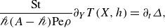 \begin{align}&\qquad\qquad\qquad\qquad \frac {\textrm{St}}{\mathscr{h}(A-\mathscr{h}) \textrm{Pe} \rho } \partial _Y T(X,h) = \partial _t \varDelta, \end{align}
where $\varDelta$
is the remaining height of the solid to be melted and
$\varDelta$
is the remaining height of the solid to be melted and $\partial _t\varDelta$
represents the melting rate.
$\partial _t\varDelta$
represents the melting rate.
In accordance with previous experimental and theoretical results (Moallemi, Webb & Viskanta Reference Moallemi, Webb and Viskanta1986; Hu & Fan Reference Hu and Fan2023), the following well-validated assumptions are adopted: (i) the lubrication approximation is valid due to $ \mathscr{h}^2 \ll 1$
; (ii) the flow is quasisteady,
$ \mathscr{h}^2 \ll 1$
; (ii) the flow is quasisteady, $\partial /\partial {t}=0$
, as a consequence of a low effective Reynolds number,
$\partial /\partial {t}=0$
, as a consequence of a low effective Reynolds number, $\textrm{Re}\mathscr{h}^2 \ll 1$
; (iii) thermophysical properties are constant; (iv) the solid–liquid interface is flat, i.e.
$\textrm{Re}\mathscr{h}^2 \ll 1$
; (iii) thermophysical properties are constant; (iv) the solid–liquid interface is flat, i.e. $ h=h(t)$
; (v) the hydrostatic pressure in the liquid film is neglected (
$ h=h(t)$
; (v) the hydrostatic pressure in the liquid film is neglected ( $p_h \ll 1$
); (vi) heat convection is negligible
$p_h \ll 1$
); (vi) heat convection is negligible $\textrm{Pe}\mathscr{h}^2 \ll 1$
when
$\textrm{Pe}\mathscr{h}^2 \ll 1$
when $\textrm{St} \leqslant 0.1$
for CCM (Hu & Fan Reference Hu and Fan2023; Ezra & Kozak Reference Ezra and Kozak2024); (vii) viscous dissipation is negligible due to
$\textrm{St} \leqslant 0.1$
for CCM (Hu & Fan Reference Hu and Fan2023; Ezra & Kozak Reference Ezra and Kozak2024); (vii) viscous dissipation is negligible due to $ \textrm{PrEc} \ll 1$
for most PCMs and thermal conditions; (viii) the initial temperature of the PCM solid remains
$ \textrm{PrEc} \ll 1$
for most PCMs and thermal conditions; (viii) the initial temperature of the PCM solid remains $T_m$
; (ix) the heat flux across the gas–liquid interface is negligible due to the much low thermal conductivity of the gas compared with the liquid. Additionally, we consider (x) the initial geometrical conditions
$T_m$
; (ix) the heat flux across the gas–liquid interface is negligible due to the much low thermal conductivity of the gas compared with the liquid. Additionally, we consider (x) the initial geometrical conditions $ \mathscr{l}^2 \ll 1$
and
$ \mathscr{l}^2 \ll 1$
and $\mathscr{h} \ll A$
. Consequently, with
$\mathscr{h} \ll A$
. Consequently, with $l =l^*/h_0^*$
providing the corresponding transverse dimensions of the liquid flow channel, the governing equations can be simplified considerably to
$l =l^*/h_0^*$
providing the corresponding transverse dimensions of the liquid flow channel, the governing equations can be simplified considerably to
 \begin{align}&\qquad \partial _Xu+\partial _Yv=0, \\[-9pt] \nonumber \end{align}
 \begin{align}& 0= -\partial _XP+\partial _Y^2u+ l^{-2}\partial _Z^2u, \\[-9pt] \nonumber \end{align}
 \begin{align}&\qquad\quad\,\, 0= \partial _YP, \\[-9pt] \nonumber \end{align}
 \begin{align}&\qquad\quad\,\, 0 = \partial _Z P, \\[-9pt] \nonumber \end{align}
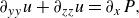
 \begin{align}&\qquad 0 = \partial _Y^2 T+l^{-2}\partial _Z^2T, \\[-9pt] \nonumber \end{align}
 \begin{align}&\qquad\, \partial _YT(X,h)= \frac {d\Delta }{d \tau }, \end{align}
where $\tau \equiv t\textrm{St}/ [\rho \textrm{Pe}\mathscr{h}(A-\mathscr{h}) ]$
is a rescaled time, which recognises that a balance of heat conduction and the heat of fusion control the dynamics. Additionally, the force balance on the remaining solid is satisfied as
$\tau \equiv t\textrm{St}/ [\rho \textrm{Pe}\mathscr{h}(A-\mathscr{h}) ]$
is a rescaled time, which recognises that a balance of heat conduction and the heat of fusion control the dynamics. Additionally, the force balance on the remaining solid is satisfied as
 \begin{equation} \int _{-1/2}^{1/2} P {\textrm d}X = \varDelta ^{\mathscr{c}}, \end{equation}
where $\mathscr{c} = 0$
represents the constant-pressure CCM mode and
$\mathscr{c} = 0$
represents the constant-pressure CCM mode and $\mathscr{c} = 1$
represents a gravity-driven configuration. Then, the boundary conditions for the velocity and temperature fields within a single periodic unit cell are given as
$\mathscr{c} = 1$
represents a gravity-driven configuration. Then, the boundary conditions for the velocity and temperature fields within a single periodic unit cell are given as
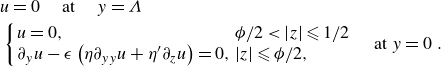
 \begin{align}& u(Y=h)=0,\ \partial _Yu(Z=\pm 1/2)=0, \ \boldsymbol{n}\cdot \nabla u(Y=0,|Z|\lt \phi /2)=0,\ u(Y=0,\notag\\&\quad |Z|\gt \phi /2)=0, \end{align}
 \begin{align}&\qquad\qquad\qquad\quad v(Y=0)=0,\ v(Y=h) = \rho A\mathscr{h}^{-1}\partial _{t} H - \partial _{ t} h, \end{align}
 \begin{align}& T(Y=h)=0,\ \partial _YT(Z=\pm 1/2)=0, \ \boldsymbol{n}\cdot \nabla T(Y=0,|Z|\lt \phi /2)=0,\ T(Y=0,\notag\\&\quad |Z|\gt \phi /2)=1. \end{align}
The goal of the subsequent parts of § 2 is to determine the flow and temperature fields so as to find how the PCM height changes with time, i.e. $\varDelta (\tau )$
or
$\varDelta (\tau )$
or $H(\tau )$
. A significant computational difficulty is to do this calculation for different groove configurations, i.e. gas–liquid fractions
$H(\tau )$
. A significant computational difficulty is to do this calculation for different groove configurations, i.e. gas–liquid fractions $\phi$
and dimensionless periodic lengths
$\phi$
and dimensionless periodic lengths $l$
and liquid film thicknesses
$l$
and liquid film thicknesses $\Lambda$
. The specific results are given in § 3.
$\Lambda$
. The specific results are given in § 3.
2.2. Average heat flux and effective thermal slip length
In this section, a dual-series approach similar to previous work (Lauga & Stone Reference Lauga and Stone2003; Sbragaglia & Prosperetti Reference Sbragaglia and Prosperetti2007; Kirk et al. Reference Kirk, Hodes and Papageorgiou2017) was adopted to give exact solutions for an effective thermal slip length $\lambda _{t}^{*}$
in the two-dimensional configuration. For convenience and consistency with previous work, the characteristic length
$\lambda _{t}^{*}$
in the two-dimensional configuration. For convenience and consistency with previous work, the characteristic length $l^{*}$
of the periodic topography of the substrate is used for the length scale throughout this section, leading to dimensionless coordinates
$l^{*}$
of the periodic topography of the substrate is used for the length scale throughout this section, leading to dimensionless coordinates $(x,y,z)\equiv (x^*,y^*,z^*)/l^*$
and channel height
$(x,y,z)\equiv (x^*,y^*,z^*)/l^*$
and channel height $\Lambda \equiv h^*/l^*$
. Consequently, the schematic diagram of the configuration is depicted in figure 1(b). The dimensionless variables
$\Lambda \equiv h^*/l^*$
. Consequently, the schematic diagram of the configuration is depicted in figure 1(b). The dimensionless variables $X$
and
$X$
and $Y$
introduced in the previous subsection will return when we obtain a one-dimensional model of the problem in § 2.4.
$Y$
introduced in the previous subsection will return when we obtain a one-dimensional model of the problem in § 2.4.
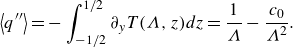
In addition to the temperature distribution, our primary interest lies in the average heat flux $\left \langle q^{\prime \prime }\right \rangle \equiv \int _{-1/2}^{1/2} -\partial _yT(\Lambda, z) dz$
through the upper boundary of the liquid film, as this parameter determines the melting rate as indicated by (2.4f
). Consequently, the introduction of an effective thermal slip length
$\left \langle q^{\prime \prime }\right \rangle \equiv \int _{-1/2}^{1/2} -\partial _yT(\Lambda, z) dz$
through the upper boundary of the liquid film, as this parameter determines the melting rate as indicated by (2.4f
). Consequently, the introduction of an effective thermal slip length $\lambda _t \equiv \lambda _t^*/l^*$
can reduce the two-dimensional problem
$\lambda _t \equiv \lambda _t^*/l^*$
can reduce the two-dimensional problem $T(y,z)$
in the
$T(y,z)$
in the $y-z$
plane to a one-dimensional problem
$y-z$
plane to a one-dimensional problem $\bar T(y)$
in the
$\bar T(y)$
in the $y$
direction, as illustrated in the schematic of the thermal transport in figure 1(b). In the following,
$y$
direction, as illustrated in the schematic of the thermal transport in figure 1(b). In the following, $\lambda _{t,f}$
and
$\lambda _{t,f}$
and $\lambda _{t,c}$
represent, respectively, the thermal slip lengths of a flat and curved gas–liquid interface.
$\lambda _{t,c}$
represent, respectively, the thermal slip lengths of a flat and curved gas–liquid interface.
2.2.1. On the flat interface, $\lambda _{t,f}$

Based on (2.4e ), the dimensionless form of the energy equation is rewritten as
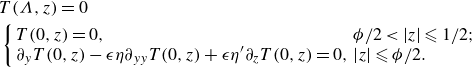
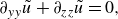
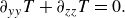 \begin{equation} \partial _{yy} T + \partial _{zz} T = 0. \end{equation}
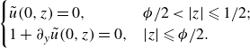
As depicted in figure 1(b), the boundary conditions are
 \begin{align}&\qquad\qquad {T}(\Lambda, z)=0, \end{align}
 \begin{align}& \begin{cases} {T}(0,z)=1, & \phi /2 \lt |z| \leqslant 1/2 \\ \partial _y {T}(0,z)= 0, & |z| \leqslant \phi /2 \end{cases} \end{align}
 \begin{align}&\,\, \partial _z T(y,-1/2)= \partial _zT(y,1/2) = 0, \end{align}
we assume that the heat flux vanishes at the gas–liquid boundary owing to the smallness of the ratio of the gas and liquid thermal conductivities. We can observe that the boundary conditions for this two-dimensional problem introduce the fraction of the boundary that involves the gas–liquid fraction $\phi$
. Due to the linearity of the boundary-value problem, the temperature
$\phi$
. Due to the linearity of the boundary-value problem, the temperature $T$
can be divided into two components
$T$
can be divided into two components $T_b$
and
$T_b$
and $T_s$
, namely
$T_s$
, namely $T(y,z)=T_b(y)+T_s(y,z)$
, where
$T(y,z)=T_b(y)+T_s(y,z)$
, where $T_b(y) = 1 - y/\Lambda$
satisfies the boundary conditions on temperature in the
$T_b(y) = 1 - y/\Lambda$
satisfies the boundary conditions on temperature in the $y$
direction, and
$y$
direction, and $T_s(y,z)=\tilde {T}(y,z)/\Lambda$
accounts for the influence of the hydrophobic surface. Hence,
$T_s(y,z)=\tilde {T}(y,z)/\Lambda$
accounts for the influence of the hydrophobic surface. Hence, $\tilde {T}$
also satisfies the Laplace equation as
$\tilde {T}$
also satisfies the Laplace equation as
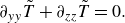 \begin{equation} \partial _{yy} \tilde {T} + \partial _{zz} \tilde {T} = 0. \end{equation}
The boundary conditions for $\tilde {T}$
are
$\tilde {T}$
are
 \begin{align}&\qquad\qquad\qquad \tilde {T}(\Lambda, z)=0, \end{align}
 \begin{align}& \begin{cases} \tilde {T}(0,z)=0, & \phi /2 \lt |z| \leqslant 1/2; \\ -1 + \partial _y\tilde {T}(0,z) = 0, & |z| \leqslant \phi /2. \end{cases} \end{align}
The general solution $\tilde {T}$
, accounting for condition (2.8c
), is
$\tilde {T}$
, accounting for condition (2.8c
), is
 \begin{equation} \begin{aligned} \tilde {T} (y, z) = c_0 \frac {y}{\Lambda } + d_0 + \sum _{n=1}^\infty \left [c_n \cosh \left (2\pi n y\right ) + d_n \sinh \left (2\pi n y\right )\right ] \cos \left (2\pi n z\right ), \end{aligned} \end{equation}
where $c_n$
and
$c_n$
and $d_n$
for
$d_n$
for $n \in [0, \infty )$
are constants to be determined for given
$n \in [0, \infty )$
are constants to be determined for given $\phi$
and
$\phi$
and $\Lambda$
. Following the standard procedure of a dual-series method to numerically solve (2.12) as detailed in Appendix A,
$\Lambda$
. Following the standard procedure of a dual-series method to numerically solve (2.12) as detailed in Appendix A, $c_n$
and
$c_n$
and $d_n$
for
$d_n$
for $n \in [0, N-1]$
can be obtained with a numerical truncation for large enough
$n \in [0, N-1]$
can be obtained with a numerical truncation for large enough $N$
. The choice of
$N$
. The choice of $N$
should be chosen to ensure convergence of the numerical results (Teo & Khoo Reference Teo and Khoo2008). Here, we adopt
$N$
should be chosen to ensure convergence of the numerical results (Teo & Khoo Reference Teo and Khoo2008). Here, we adopt $N=500$
as there is no significant deviation with
$N=500$
as there is no significant deviation with $N=1000$
, which is also consistent with Landel et al. (Reference Landel, Peaudecerf, Temprano-Coleto, Gibou, Goldstein and Luzzatto-Fegiz2020). Therefore, the average heat flux
$N=1000$
, which is also consistent with Landel et al. (Reference Landel, Peaudecerf, Temprano-Coleto, Gibou, Goldstein and Luzzatto-Fegiz2020). Therefore, the average heat flux $\left \langle q^{\prime \prime }\right \rangle$
can be calculated by substituting
$\left \langle q^{\prime \prime }\right \rangle$
can be calculated by substituting $c_0$
as
$c_0$
as
 \begin{equation} \left \langle q^{\prime \prime }\right \rangle = -\int _{-1/2}^{1/2} \partial _yT(\Lambda, z) dz = \frac {1}{\Lambda } - \frac {c_0}{\Lambda ^2}. \end{equation}
The definition of an effective thermal slip length $ \lambda _{t}$
representative of the composite flat liquid–gas surface and solid–liquid surface (Enright et al. Reference Enright, Hodes, Salamon and Muzychka2014) is
$ \lambda _{t}$
representative of the composite flat liquid–gas surface and solid–liquid surface (Enright et al. Reference Enright, Hodes, Salamon and Muzychka2014) is
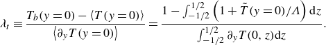 \begin{equation} \lambda _{t} \equiv \frac {T_b(y=0)- \left \langle T(y=0)\right \rangle }{\left \langle \partial _y T(y=0)\right \rangle } = \frac {1-\int _{-1/2}^{1/2}\left (1+\tilde {T}(y=0)/\Lambda \right ){\textrm d} z}{\int _{-1/2}^{1/2} \partial _yT(0, z) {\textrm d}z}. \end{equation}
With the results of $1-\int _{-1/2}^{1/2}(1+\tilde {T}(y=0)/\Lambda ) {\textrm d}z= c_0/\Lambda$
due to
$1-\int _{-1/2}^{1/2}(1+\tilde {T}(y=0)/\Lambda ) {\textrm d}z= c_0/\Lambda$
due to $c_0 = -d_0$
from Appendix A and
$c_0 = -d_0$
from Appendix A and $\int _{-1/2}^{1/2} \partial _yT(0, z) {\textrm d}z= \left \langle q^{\prime \prime }\right \rangle$
, we find the effective thermal slip length
$\int _{-1/2}^{1/2} \partial _yT(0, z) {\textrm d}z= \left \langle q^{\prime \prime }\right \rangle$
, we find the effective thermal slip length $ \lambda _{t,f}$
for a flat, composite gas–liquid interface:
$ \lambda _{t,f}$
for a flat, composite gas–liquid interface:
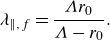
 \begin{equation} \begin{aligned} \lambda _{t,f} = \frac {{\Lambda }c_0}{\Lambda -c_0}. \end{aligned} \end{equation}
2.2.2. On the curved interface,
$\lambda _{t,c}$

We next consider how the deformation of the gas–liquid interface affects the thermal slip length. A curved liquid–air interface is formed by the pressure difference between liquid $ P_l^{*}$
and gas
$ P_l^{*}$
and gas $ P_g^{*}$
, and described approximately by the radius of curvature
$ P_g^{*}$
, and described approximately by the radius of curvature $ R^{*} = \sigma ^{*}/(P_l^{*} - P_g^{*})$
, where
$ R^{*} = \sigma ^{*}/(P_l^{*} - P_g^{*})$
, where $\sigma ^{*}$
is the surface tension. Hence, the shape of the meniscus can be described by the geometric relationship
$\sigma ^{*}$
is the surface tension. Hence, the shape of the meniscus can be described by the geometric relationship
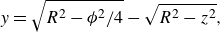 \begin{equation} y = \sqrt {R^2 - \phi ^2 / 4} - \sqrt {R^2 - z^2}, \end{equation}
where $R = R^{*} / l^{*}$
. For
$R = R^{*} / l^{*}$
. For $R \gg \phi / 2$
, this expression simplifies to
$R \gg \phi / 2$
, this expression simplifies to
 \begin{equation} y = \frac {1}{8R} \left (4z^2 - \phi ^2\right ) + {O}\left (\frac {1}{R^3}\right ) = - \epsilon \eta (z) \quad \text{for} \quad |z| \leqslant \phi / 2, \end{equation}
after defining $\epsilon = 1 / (8R)$
, which will be assumed
$\epsilon = 1 / (8R)$
, which will be assumed $\ll 1$
, and
$\ll 1$
, and $\eta (z) = \phi ^2 - 4z^2$
. It should be noted that the protrusion angle
$\eta (z) = \phi ^2 - 4z^2$
. It should be noted that the protrusion angle $\theta$
satisfies
$\theta$
satisfies $R \sin \theta = \phi / 2$
, which leads to a maximum
$R \sin \theta = \phi / 2$
, which leads to a maximum $\epsilon = \sin \theta /4\phi = 0.217$
for
$\epsilon = \sin \theta /4\phi = 0.217$
for $\phi = 0.2$
and
$\phi = 0.2$
and $\theta = 10^{\circ }$
. Again, neglecting the influence of the conductivity of the gas phase, then we have the condition of no heat flux across the meniscus, and the temperature field should satisfy
$\theta = 10^{\circ }$
. Again, neglecting the influence of the conductivity of the gas phase, then we have the condition of no heat flux across the meniscus, and the temperature field should satisfy
 \begin{equation} \boldsymbol{n} \cdot \boldsymbol{\nabla }T = 0 \quad \text{at} \quad y =-\epsilon \eta (z), \end{equation}
which is equivalent to
 \begin{equation} \partial _y T(-\epsilon \eta, z)+\epsilon \eta ^{\prime } \partial _z T(-\epsilon \eta, z)=0, \end{equation}
where $\eta ^{\prime } \equiv \textrm{d} \eta /\textrm{d}z =-8z$
. Since
$\eta ^{\prime } \equiv \textrm{d} \eta /\textrm{d}z =-8z$
. Since $\epsilon \ll 1$
,
$\epsilon \ll 1$
, $T(-\epsilon \eta, z)$
can be obtained from
$T(-\epsilon \eta, z)$
can be obtained from $T(0, z)$
by Taylor expansion as
$T(0, z)$
by Taylor expansion as $T(-\epsilon \eta, z)=T(0, z)-\epsilon \eta \partial _y T(0, z)+O (\epsilon ^2 )$
, leading to
$T(-\epsilon \eta, z)=T(0, z)-\epsilon \eta \partial _y T(0, z)+O (\epsilon ^2 )$
, leading to
 \begin{equation} \begin{aligned} & \partial _y T(-\epsilon \eta, z)=\partial _y T(0, z)-\epsilon \eta \partial _{yy} T(0, z)+O(\epsilon ^2), \\ & \partial _z T(-\epsilon \eta, z)=\partial _z T(0, z)+O(\epsilon ). \end{aligned} \end{equation}
Then, substitution of (2.20) into (2.19) yields
 \begin{equation} \partial _y T(0, z)-\epsilon \eta \partial _{yy} T(0, z)+\epsilon \eta ^{\prime } \partial _z T(0, z)+O(\epsilon ^2)=0. \end{equation}
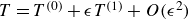
Hence, the boundary conditions are
 \begin{equation} \begin{aligned} & T(\Lambda, z)=0 \\ & \left \{\begin{array}{ll} T(0, z)=0, & \phi /2\lt |z| \leqslant 1 / 2; \\ \partial _y T(0, z)-\epsilon \eta \partial _{y y} T(0, z)+\epsilon \eta ^{\prime } \partial _z T(0, z)=0, & |z| \leqslant \phi /2. \end{array} \right . \end{aligned} \end{equation}
After a perturbation analysis by substituting $T=T^{(0)}+\epsilon T^{(1)}+O (\epsilon ^2 )$
(details provided in Appendix B), we find that the presence of a curved gas–liquid interface has no influence on the average heat flux and thermal slip length, which means
$T=T^{(0)}+\epsilon T^{(1)}+O (\epsilon ^2 )$
(details provided in Appendix B), we find that the presence of a curved gas–liquid interface has no influence on the average heat flux and thermal slip length, which means
 \begin{equation} \lambda _{t,f}=\lambda _{t,c}\equiv \lambda _t. \end{equation}
We have now completed the necessary aspects of the thermal problem inside the thin film to estimate the time variations of the PCM, which will be described in § 2.4.
2.3. Flow rate – pressure gradient relationship and velocity slip length
We now consider the flow in the thin film since we need the pressure distribution to complete the force balance on the PCM. Based on (2.4b
)–(2.4d
), the main liquid flow is along the $x$
direction as indicated in figure 1(d). Similar to § 2.2, in addition to obtaining the velocity field
$x$
direction as indicated in figure 1(d). Similar to § 2.2, in addition to obtaining the velocity field $u$
, we also focus on the variation of the flow rate-pressure gradient relationship
$u$
, we also focus on the variation of the flow rate-pressure gradient relationship $Q-\partial _x P$
due to the presence of trapped gas, which will influence the pressure distribution within the liquid film and the liquid film thickness during the CCM process. By introducing the velocity slip length
$Q-\partial _x P$
due to the presence of trapped gas, which will influence the pressure distribution within the liquid film and the liquid film thickness during the CCM process. By introducing the velocity slip length $\lambda \equiv \lambda ^*/l^*$
to enable an equivalent flow rate
$\lambda \equiv \lambda ^*/l^*$
to enable an equivalent flow rate $\bar Q = Q$
as demonstrated in figure 1(e), these steps allow a dimensional reduction from
$\bar Q = Q$
as demonstrated in figure 1(e), these steps allow a dimensional reduction from $u(y,z)$
to
$u(y,z)$
to $\bar u(y)$
. In the following,
$\bar u(y)$
. In the following, $\lambda _{\parallel, f}$
and
$\lambda _{\parallel, f}$
and $\lambda _{\parallel, c}$
represent the velocity slip lengths by flat and curved gas–liquid interfaces, respectively, while the main liquid flow is parallel to the orientation of the grooves.
$\lambda _{\parallel, c}$
represent the velocity slip lengths by flat and curved gas–liquid interfaces, respectively, while the main liquid flow is parallel to the orientation of the grooves.
2.3.1. Velocity slip length on the flat interface,
$\lambda _{\parallel, f}$

With the definition of variables introduced in the previous section, the dimensionless form of the momentum equation is
 \begin{equation} \partial _{yy}u+\partial _{zz}u=\partial _xP, \end{equation}
where $u={u}^{*} \mu ^{*} L^{*}/({{l}^{*}}^2p_c^{*})$
. Due to linearity, the velocity
$u={u}^{*} \mu ^{*} L^{*}/({{l}^{*}}^2p_c^{*})$
. Due to linearity, the velocity $u(y,z)$
can be divided into two components
$u(y,z)$
can be divided into two components $u_b(y)$
and
$u_b(y)$
and $u_{s}(y,z)$
, where
$u_{s}(y,z)$
, where $u_b(y) = -\partial _xP (\Lambda y-y^2 )/2$
accounts for the flow without slip and
$u_b(y) = -\partial _xP (\Lambda y-y^2 )/2$
accounts for the flow without slip and $u_s(y,z)=-\partial _xP\Lambda \tilde {u}/2$
accounts for slip along the hydrophobic surface. Hence, substituting
$u_s(y,z)=-\partial _xP\Lambda \tilde {u}/2$
accounts for slip along the hydrophobic surface. Hence, substituting $u(y,z)= -\partial _xP (\Lambda y-y^2+\Lambda \tilde {u}(y,z) )/2$
leads to a boundary-value problem
$u(y,z)= -\partial _xP (\Lambda y-y^2+\Lambda \tilde {u}(y,z) )/2$
leads to a boundary-value problem
 \begin{equation} \partial _{yy} \tilde {u}+\partial _{zz} \tilde {u}=0, \end{equation}
with corresponding homogeneous boundary conditions
 \begin{align}&\qquad\qquad\quad \tilde {u}(\Lambda, z)=0, \end{align}
 \begin{align}& \begin{cases}\tilde {u}(0, z)=0, & \phi /2 \lt |z| \leqslant 1/2; \\ 1+\partial _{y} \tilde {u}(0, z)=0, & |z|\leqslant \phi /2.\end{cases} \end{align}
This problem is effectively identical to the thermal problem in § 2.2.1. The general solution of $\tilde {u}(y,z)$
with periodic boundary conditions at
$\tilde {u}(y,z)$
with periodic boundary conditions at $z = \pm 1/2$
is
$z = \pm 1/2$
is
 \begin{equation} \begin{aligned} \tilde {u} (y,z) = r_0 +q_{0}\frac {y}{\Lambda }+\sum _{n=1}^\infty \left [r_n\cosh \left (2\pi n y\right )+q_n \sinh \left (2\pi n y\right )\right ] \cos \left (2\pi n z\right ), \end{aligned} \end{equation}
where constants $r_n$
and
$r_n$
and $q_n$
(
$q_n$
( $n \in [0, N-1]$
), dependent on
$n \in [0, N-1]$
), dependent on $\phi$
and
$\phi$
and $\Lambda$
, also can be numerically determined similar to the dual-series approach in Appendix C. Consequently, the increased flow rate
$\Lambda$
, also can be numerically determined similar to the dual-series approach in Appendix C. Consequently, the increased flow rate $Q_d$
due to the presence of slip can be obtained via
$Q_d$
due to the presence of slip can be obtained via
 \begin{equation} Q_d = \int _{0}^{\Lambda }\int _{-1/2}^{1/2} u_s \textrm{d}z\textrm{d}y =\int _{0}^{\Lambda }\int _{-1/2}^{1/2} -\frac {{\textrm d}P}{{\textrm d}x}\frac {\Lambda \tilde {u}}{2} \textrm{d}z\textrm{d}y= -\frac {{\textrm d}P}{{\textrm d}x}\frac {{\Lambda }^2r_0}{4}. \end{equation}
On the other hand, for a model pressure-driven channel flow with one boundary of slip length $\lambda$
, the increased flow rate
$\lambda$
, the increased flow rate $Q_d$
can be written as
$Q_d$
can be written as
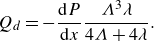 \begin{equation} Q_d = -\frac {{\textrm d}P}{{\textrm d}x}\frac {{\Lambda ^3\lambda }}{4\Lambda +4\lambda }. \end{equation}
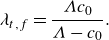
Comparing the last two expressions, the effective velocity slip length $\lambda _{\parallel, f}$
on the longitudinal grooves for a flat liquid–gas interface is
$\lambda _{\parallel, f}$
on the longitudinal grooves for a flat liquid–gas interface is
 \begin{equation} \lambda _{\parallel, f} = \frac {\Lambda r_0}{\Lambda -r_0}. \end{equation}
A reader should notice that the detailed boundary value problems for the thermal and velocity fields, and corresponding dual integral equations solutions, show that the two problems are identical, $r_n=-c_n$
and
$r_n=-c_n$
and $r_0=c_0$
. Thus,
$r_0=c_0$
. Thus, $\lambda _{\parallel, f}=\lambda _{t,f}$
as evident from (2.31) and (2.15).
$\lambda _{\parallel, f}=\lambda _{t,f}$
as evident from (2.31) and (2.15).
2.3.2. Velocity slip length on the curved interface,
$\lambda _{\parallel, c}$

To account for a curved gas–liquid interface, we consider the configuration similar to § 2.2.2. In order to satisfy the condition of zero shear stress at the steady-state gas–liquid interface, the velocity should satisfy
 \begin{equation} \boldsymbol{n} \cdot \boldsymbol{\nabla }u = 0 \quad \text{at} \quad y =-\epsilon \eta, \end{equation}
which is equivalent to
 \begin{equation} \epsilon \eta ^{\prime } \partial _z u(-\epsilon \eta, z)+\partial _y u(-\epsilon \eta, z)=0. \end{equation}
Since $\epsilon \ll 1$
,
$\epsilon \ll 1$
, $u(-\epsilon \eta, z)$
can be obtained from
$u(-\epsilon \eta, z)$
can be obtained from $u(y, z)$
by Taylor expansion as
$u(y, z)$
by Taylor expansion as $u(-\epsilon \eta, z)=u(0, z)-\epsilon \eta \partial _y u(0, z)+O (\epsilon ^2 )$
as
$u(-\epsilon \eta, z)=u(0, z)-\epsilon \eta \partial _y u(0, z)+O (\epsilon ^2 )$
as
 \begin{align}& \partial _y u(-\epsilon \eta, z)=\partial _y u(0, z)-\epsilon \eta \partial _{yy} u(0, z)+O(\epsilon ^2), \end{align}
 \begin{align}&\qquad\quad \partial _z u(-\epsilon \eta, z)=\partial _z u(0, z)+O(\epsilon ). \end{align}
Then, substitution of (2.34a ) and (2.34b ) into (2.33) yields
 \begin{equation} \partial _y u(0, z)-\epsilon \eta \partial _{yy} u(0, z)+\epsilon \eta ^{\prime } \partial _z u(0, z)+O(\epsilon ^2)=0. \end{equation}
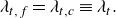
Hence, the boundary conditions are
 \begin{equation} \begin{aligned} & u=0 \quad \text{ at } \quad y=\Lambda \\ & \left \{\begin{array}{ll} u=0, & \phi /2\lt |z| \leqslant 1 / 2 \\ \partial _y u-\epsilon \left ( \eta \partial _{y y} u+ \eta ^{\prime } \partial _z u\right )=0, & |z| \leqslant \phi /2, \end{array} \quad\text{ at } y=0\right . . \end{aligned} \end{equation}
After substituting the perturbation expansion for the velocity field, $u=u^{(0)}+\epsilon u^{(1)}+O (\epsilon ^2 )$
, we solve for the first-order velocity
$u=u^{(0)}+\epsilon u^{(1)}+O (\epsilon ^2 )$
, we solve for the first-order velocity $\tilde {u}^{(1)}$
(see Appendix D) as
$\tilde {u}^{(1)}$
(see Appendix D) as
 \begin{equation} \tilde {u}^{(1)}=r_0^{(1)} +q_0^{(1)}\frac {y}{\Lambda }+\sum _{n=1}^{\infty }\left [r_n^{(1)} \cosh \left (2\pi n y\right )+q_n^{(1)} \sinh \left (2\pi n y\right )\right ] \cos \left (2\pi n z\right )\!; \end{equation}
the coefficients $r_0^{(0)}$
,
$r_0^{(0)}$
, $r_n^{(0)}$
,
$r_n^{(0)}$
, $r_0^{(1)}$
, and
$r_0^{(1)}$
, and $r_n^{(1)}$
can be obtained numerically. Consequently, the total flow rate
$r_n^{(1)}$
can be obtained numerically. Consequently, the total flow rate $Q$
can be calculated as
$Q$
can be calculated as
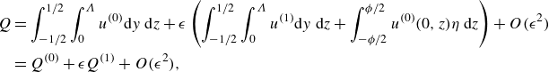 \begin{equation} \begin{aligned} Q & =\int _{-1/2}^{ 1/2} \int _{0}^{\Lambda } u^{(0)} \textrm{d} y \textrm{\ d} z+\epsilon \left (\int _{-1/2}^{ 1/2} \int _{0}^{\Lambda } u^{(1)} \textrm{d} y \textrm{\ d} z+\int _{-\phi /2}^{\phi /2} u^{(0)}(0, z) \eta \textrm{\ d} z\right )+O(\epsilon ^2) \\ &=Q^{(0)}+\epsilon Q^{(1)}+O(\epsilon ^2), \end{aligned} \end{equation}
where
 \begin{align}&\qquad\qquad\qquad\qquad\quad Q^{(0)} = -\frac {dP}{dx}\left [\frac {{\Lambda }^3}{12}+\frac {{\Lambda }^2r_0^{(0)}}{4}\right ], \end{align}
 \begin{align}& Q^{(1)} = -\frac {dP}{dx}\left [\frac {{\Lambda }^2r_0^{(1)}}{4}+ \frac {\phi ^3\Lambda }{3}r_0^{(0)}+\Lambda \sum _{n=1}^{\infty } r_n^{(0)} \frac {\sin (n\pi \phi )-n\pi \phi \cos (n\pi \phi )}{n^3\pi ^3} \right ]. \end{align}
Based on $Q=-\partial _xP\Lambda ^3/12+Q_d = -\partial _xP\Lambda ^3/12 -\partial _xP\Lambda ^3\lambda /(4\Lambda +4\lambda )$
, the slip length
$Q=-\partial _xP\Lambda ^3/12+Q_d = -\partial _xP\Lambda ^3/12 -\partial _xP\Lambda ^3\lambda /(4\Lambda +4\lambda )$
, the slip length $\lambda _{\parallel, c}$
along the curved interface is
$\lambda _{\parallel, c}$
along the curved interface is
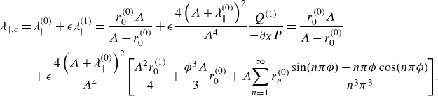 \begin{equation} \begin{aligned} \lambda _{\parallel, c} &= \lambda _{\parallel }^{(0)} + \epsilon \lambda _{\parallel }^{(1)} = \frac {r_0^{(0)}\Lambda }{\Lambda - r_0^{(0)}} + \epsilon \frac {4\left (\Lambda + \lambda _{\parallel }^{(0)}\right )^2}{{\Lambda }^4}\frac {Q^{(1)}}{-\partial _X P} = \frac {r_0^{(0)}\Lambda }{\Lambda - r_0^{(0)}} \\ & \quad + \epsilon \frac {4\left (\Lambda + \lambda _{\parallel }^{(0)}\right )^2}{{\Lambda }^4}\!\left [ \! \frac {{\Lambda }^2 r_0^{(1)}}{4} + \frac {\phi ^3 \Lambda }{3} r_0^{(0)} + \Lambda \! \sum _{n=1}^{\infty } r_n^{(0)} \frac {\sin (n\pi \phi )-n\pi \phi \cos (n\pi \phi )}{n^3\pi ^3} \! \right ]\!. \end{aligned} \end{equation}
2.4. A one-dimensional description of CCM with slip
The velocity slip length $\lambda \equiv \lambda ^*/l^*$
and temperature slip length
$\lambda \equiv \lambda ^*/l^*$
and temperature slip length $\lambda _{t}\equiv \lambda _t^*/l^*$
, describing average effects from the mixed boundary conditions of the two-dimensional problem, enable us to simplify the CCM problem into an effective one-dimensional problem describing flow and heat exchange along the direction of liquid flow, shown in the schematic diagram in figure 1(f), where the notation
$\lambda _{t}\equiv \lambda _t^*/l^*$
, describing average effects from the mixed boundary conditions of the two-dimensional problem, enable us to simplify the CCM problem into an effective one-dimensional problem describing flow and heat exchange along the direction of liquid flow, shown in the schematic diagram in figure 1(f), where the notation $ \bar {()}$
implies that the variables are averaged in the
$ \bar {()}$
implies that the variables are averaged in the $z$
direction. The corresponding governing equations (2.4a
), (2.4b
), (2.4e
) and (2.4f
) can be replaced, respectively, by
$z$
direction. The corresponding governing equations (2.4a
), (2.4b
), (2.4e
) and (2.4f
) can be replaced, respectively, by
 \begin{align}&\,\, \partial _X \bar u +\partial _Y \bar v = 0, \end{align}
 \begin{align}& 0=-\partial _X \bar P+\partial _Y^2 \bar u, \end{align}
 \begin{align}&\qquad 0=\partial _Y^2 \bar T, \end{align}
 \begin{align}& \partial _Y \bar T(X,h)= \frac {{\textrm d}\Delta }{{\textrm d} \tau } . \end{align}
Hence, the corresponding boundary conditions in figure 1(f) are
 \begin{align}&\qquad\qquad\qquad \bar u(X,0) = l\lambda \partial _Y \bar u(X,0), \quad \bar u(X,h)=0, \end{align}
 \begin{align}&\qquad\qquad 1-\bar T(X,0)=-l\lambda _{t}\partial _Y \bar T(X,0), \quad \bar T(X,h)=0, \end{align}
 \begin{align}& \bar v(X,0)=0,\quad \bar v(X,h)=\left [ \left (A-{\mathscr{h}}\right )\frac {\rho }{\mathscr{h}}\frac {{\textrm d} \Delta }{{\textrm d} \tau }+\left (\rho -1\right )\frac {{\textrm d} h}{{\textrm d} \tau }\right ]\frac {\textrm{St}}{\rho \textrm{Pe}\mathscr{h}\left (A-\mathscr{h}\right )}, \end{align}
 \begin{align}&\qquad\qquad\qquad\qquad \partial _X \bar P(0,Y)=0, \quad \bar P(1/2,Y)=0. \end{align}
It is worth noting that the upper velocity boundary $\bar v(X,h)$
is derived from
$\bar v(X,h)$
is derived from $\bar v^*(x^*,h^*) = \rho \partial _{t^*} H^* - \partial _{ t^*} h^*$
based on mass conservation at the melting front.
$\bar v^*(x^*,h^*) = \rho \partial _{t^*} H^* - \partial _{ t^*} h^*$
based on mass conservation at the melting front.
The velocity profile $\bar u(X,Y)$
can be obtained by integrating (2.41b
) twice with respect to
$\bar u(X,Y)$
can be obtained by integrating (2.41b
) twice with respect to $Y$
and applying boundary conditions (2.42a
), yielding
$Y$
and applying boundary conditions (2.42a
), yielding
 \begin{equation} \bar u = \frac {h^2}{2}\frac {\partial \bar P}{\partial X}\left (\frac {Y^2}{h^2}-\frac {Y/l+\lambda }{\Lambda +\lambda }\right ), \end{equation}
where $ h/l = \Lambda$
. Then, substituting (2.43) into the continuity equation (2.41a
) and integrating along
$ h/l = \Lambda$
. Then, substituting (2.43) into the continuity equation (2.41a
) and integrating along $y$
from 0 to
$y$
from 0 to $h$
leads to
$h$
leads to
 \begin{equation} \frac {h^2}{2}\frac {\partial ^2 \bar P}{\partial X^2}\int _{0}^{h}\left (\frac {Y^2}{h^2}-\frac {Y/l+\lambda }{\Lambda +\lambda }\right ) {\textrm d}Y+ \underbrace {\int _{0}^{h}\frac {\partial v}{\partial Y} {\textrm d}Y}_{\bar v|_{Y=h}-\bar v|_{Y=0}}=0. \end{equation}
Noting that $\bar v(X,h) \approx \textrm{St} \partial _\tau \varDelta /(\textrm{Pe}\mathscr{h}^2)$
due to the typical property
$\bar v(X,h) \approx \textrm{St} \partial _\tau \varDelta /(\textrm{Pe}\mathscr{h}^2)$
due to the typical property $\rho -1 \lt {O}(10^{-1})$
, then substituting (2.42c
) into (2.44) leads to
$\rho -1 \lt {O}(10^{-1})$
, then substituting (2.42c
) into (2.44) leads to
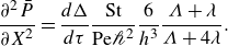 \begin{equation} \frac {\partial ^2 \bar P}{\partial X^2} = \frac {d \Delta }{d\tau } \frac {\textrm{St}}{\textrm{Pe}\mathscr{h}^2}\frac {6}{h^3}\frac {\Lambda +\lambda }{\Lambda +4\lambda } . \end{equation}
The pressure distribution can be obtained by integrating (2.45) twice with respect to $x$
, and using conditions (2.42d
), to obtain
$x$
, and using conditions (2.42d
), to obtain
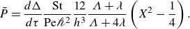 \begin{equation} \bar P = \frac {d \Delta }{d\tau } \frac {\textrm{St}}{\textrm{Pe}\mathscr{h}^2}\frac {12}{h^3}\frac {\Lambda +\lambda }{\Lambda +4\lambda } \left (X^2-\frac {1}{4}\right ). \end{equation}
Then, we can substitute (2.46) into the force balance (2.5) to obtain a relationship between $\varDelta$
and
$\varDelta$
and $h$
:
$h$
:
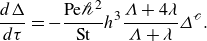 \begin{equation} \frac {d \Delta }{d\tau } = -\frac {\textrm{Pe}\mathscr{h}^2}{\textrm{St}}h^3\frac {\Lambda +4\lambda }{\Lambda +\lambda } \varDelta ^{\mathscr{c}}. \end{equation}
The temperature profile can be obtained by substituting (2.42b ) into (2.41c ), yielding
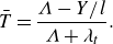 \begin{equation} \bar T = \frac {\Lambda -Y/l}{\Lambda +\lambda _{t}}. \end{equation}
Substitution of (2.48) into (2.41d ) gives
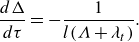 \begin{equation} \frac {d\Delta }{d\tau }=-\frac {1}{l(\Lambda +\lambda _{t})}. \end{equation}
The combination of (2.47) and (2.49) leads to
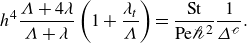 \begin{equation} h^4\frac {\Lambda +4\lambda }{\Lambda +\lambda }\left (1+\frac {\lambda _{t}}{\Lambda }\right )=\frac {\textrm{St}}{\textrm{Pe} \mathscr{h}^2}\frac {1}{\varDelta ^{\mathscr{c}}}. \end{equation}
Equations (2.49) and (2.50) are coupled expressions between the solid height $\varDelta (\tau )$
that remains and the film thickness
$\varDelta (\tau )$
that remains and the film thickness $h$
. Note that because of the definition
$h$
. Note that because of the definition $\Lambda =h/l$
where
$\Lambda =h/l$
where $l$
is fixed,
$l$
is fixed, $h$
varies with
$h$
varies with $\tau$
.
$\tau$
.
Recalling $\mathscr{h}=h_0^*/L^*$
and
$\mathscr{h}=h_0^*/L^*$
and $h=h^*/h_0^*$
in (2.1) indicates that
$h=h^*/h_0^*$
in (2.1) indicates that $h_0^*$
has not been specified. Usually, the initial height satisfies
$h_0^*$
has not been specified. Usually, the initial height satisfies $ H_0^* \gg h^*$
(i.e.
$ H_0^* \gg h^*$
(i.e. $\varDelta \approx H$
) and we can further find a characteristic initial film thickness
$\varDelta \approx H$
) and we can further find a characteristic initial film thickness $h_0^*$
that satisfies the
$h_0^*$
that satisfies the $\textrm{St}/\textrm{Pe}\mathscr{h}^2=1$
, corresponding to the initial solid height
$\textrm{St}/\textrm{Pe}\mathscr{h}^2=1$
, corresponding to the initial solid height $H=1$
and no-slip surface
$H=1$
and no-slip surface $\lambda =\lambda _t=0$
. This enables us to define
$\lambda =\lambda _t=0$
. This enables us to define $h_0^*$
as
$h_0^*$
as
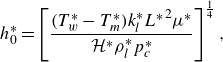 \begin{equation} h_0^* = \left [\frac {(T_w^*-T_m^*)k_l^*{L^*}^2\mu ^*}{\mathcal{H}^*\rho _l^*p_c^*}\right ]^{\frac {1}{4}}, \end{equation}
from which (2.50) and (2.49) are transformed into the equations ( $\Lambda =h/l$
)
$\Lambda =h/l$
)
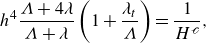 \begin{align}& h^4\frac {\Lambda +4\lambda }{\Lambda +\lambda }\left (1+\frac {\lambda _{t}}{\Lambda }\right ) = \frac {1}{H^{\mathscr{c}}}, \end{align}
 \begin{align}&\quad \frac {{\textrm d}H}{{\textrm d}\tau } = -\frac {1}{l(\Lambda +\lambda _{t})}. \end{align}
Based on (2.52a
), we can conclude that a constant film thickness $h$
is maintained for the constant-pressure mode (
$h$
is maintained for the constant-pressure mode ( $\mathscr{c}=0$
) though
$\mathscr{c}=0$
) though $\lambda$
and
$\lambda$
and $\lambda _t$
are dependent on
$\lambda _t$
are dependent on $h$
. On the other hand, for the gravity-driven mode (
$h$
. On the other hand, for the gravity-driven mode ( $\mathscr{c}=1$
) there is a coupling between
$\mathscr{c}=1$
) there is a coupling between $h$
and
$h$
and $H$
, making the solutions of
$H$
, making the solutions of $H(\tau )$
and
$H(\tau )$
and $h(\tau )$
complicated.
$h(\tau )$
complicated.
Furthermore, we introduce the Nusselt number, $\textrm{Nu}$
, based on the instantaneous height of the liquid film
$\textrm{Nu}$
, based on the instantaneous height of the liquid film $h^*(t^*)$
, to demonstrate the heat transfer capability under different conditions.
$h^*(t^*)$
, to demonstrate the heat transfer capability under different conditions. $\textrm{Nu}$
is defined as
$\textrm{Nu}$
is defined as
 \begin{equation} {\textrm{Nu}} \equiv -\frac {k_l^{*}\partial _{y^{*}} \bar T^{*}(0,h^{*})}{\left (T_w^{*}-T_m^{*}\right )}\frac {h^{*}}{k_{l}^{*}} = \frac {1}{l(\Lambda + \lambda _{t})}. \end{equation}
At this stage, we have completed all of the analysis of the thin-film flow and heat transfer necessary for modelling CCM processes, which may be enhanced using a corrugated substrate. The main variables that dictate performance are the slip lengths $\lambda$
and
$\lambda$
and $\lambda _t$
, geometric ratios
$\lambda _t$
, geometric ratios $l$
and
$l$
and $\Lambda$
, the latter which changes in time, and the resulting
$\Lambda$
, the latter which changes in time, and the resulting $\textrm{Nu}$
, which determines the melting rate, i.e. the power density of the CCM.
$\textrm{Nu}$
, which determines the melting rate, i.e. the power density of the CCM.
3. Results and discussions
The goal of this section is to calculate the melting rate (i.e. $\textrm{Nu}$
) or the instantaneous solid height (i.e.
$\textrm{Nu}$
) or the instantaneous solid height (i.e. $H(\tau )$
), which is a complicated function of geometric parameters (
$H(\tau )$
), which is a complicated function of geometric parameters ( $l$
) and slip lengths (
$l$
) and slip lengths ( $\lambda$
,
$\lambda$
, $\lambda _t$
). It also depends on the operation controlled by hydrostatic pressure or a constant applied pressure. The subsections that follow summarise the main results for different cases.
$\lambda _t$
). It also depends on the operation controlled by hydrostatic pressure or a constant applied pressure. The subsections that follow summarise the main results for different cases.
3.1. Confinement and meniscus effects on the slip length
3.1.1. Velocity slip length
$\lambda$
and temperature slip length
$\lambda _t$
at a flat interface


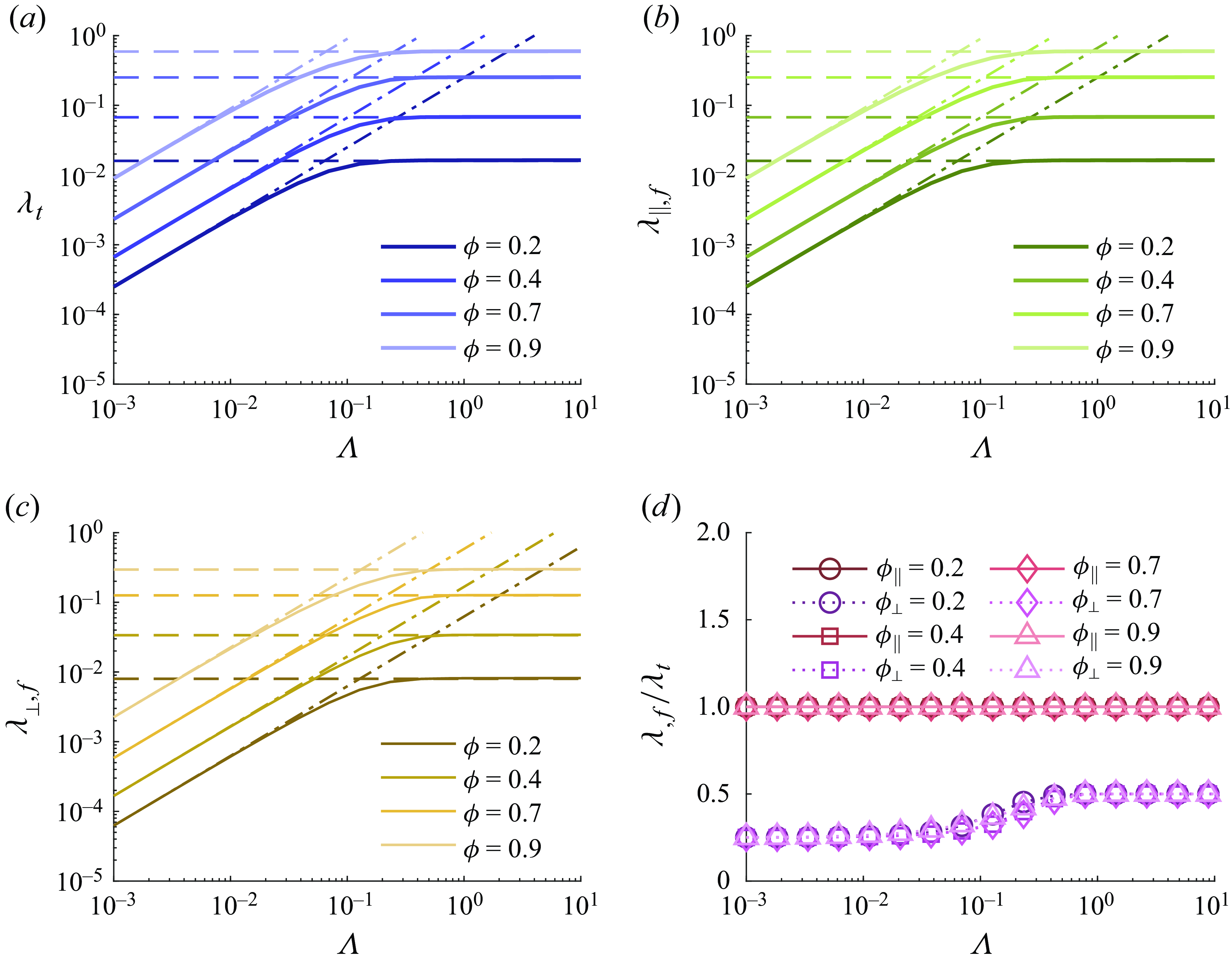
Figure 2. Slip lengths as a function of $\Lambda$
. (a) Temperature slip length
$\Lambda$
. (a) Temperature slip length $\lambda _t$
, (b) velocity slip length
$\lambda _t$
, (b) velocity slip length $\lambda _{\parallel, f}$
on longitudinal grooves and (c)
$\lambda _{\parallel, f}$
on longitudinal grooves and (c) $\lambda _{\perp, f}$
on transverse grooves versus the aspect ratio
$\lambda _{\perp, f}$
on transverse grooves versus the aspect ratio $\Lambda =h^*/l^*$
when the liquid–gas interface is flat. (d) Comparison of the ratio of the velocity to temperature slip lengths,
$\Lambda =h^*/l^*$
when the liquid–gas interface is flat. (d) Comparison of the ratio of the velocity to temperature slip lengths, $\lambda _{,f}/\lambda _t$
, between longitudinal and transverse grooves. In figures (a)–(c) the solid lines are numerical results. Dashed lines and dot–dash lines are asymptotic solutions.
$\lambda _{,f}/\lambda _t$
, between longitudinal and transverse grooves. In figures (a)–(c) the solid lines are numerical results. Dashed lines and dot–dash lines are asymptotic solutions.
The temperature $\lambda _t$
(§ 2.2.1) and velocity
$\lambda _t$
(§ 2.2.1) and velocity $\lambda _{\parallel, f}$
slip lengths (§ 2.3.1) as a function of the aspect ratio
$\lambda _{\parallel, f}$
slip lengths (§ 2.3.1) as a function of the aspect ratio $\Lambda =h^*(t^*)/l^*$
(see figure 1
a), for a given gas–liquid fraction
$\Lambda =h^*(t^*)/l^*$
(see figure 1
a), for a given gas–liquid fraction $\phi$
, are presented as solid lines in figures 2(a) and 2(b), respectively. For comparison, we also calculate the slip length
$\phi$
, are presented as solid lines in figures 2(a) and 2(b), respectively. For comparison, we also calculate the slip length $\lambda _{\perp, f}$
variation on a surface of transverse grooves in Appendix F, and present it in figure 2(c). It can be observed that across a wide range of gas–liquid fractions
$\lambda _{\perp, f}$
variation on a surface of transverse grooves in Appendix F, and present it in figure 2(c). It can be observed that across a wide range of gas–liquid fractions $\phi$
, each slip length of
$\phi$
, each slip length of $\lambda _t$
,
$\lambda _t$
, $\lambda _{\parallel, f}$
and
$\lambda _{\parallel, f}$
and $\lambda _{\perp, f}$
maintains a specific fixed value for
$\lambda _{\perp, f}$
maintains a specific fixed value for $\Lambda \gg 1$
, and exhibits a scaling law of
$\Lambda \gg 1$
, and exhibits a scaling law of $\sim \Lambda$
when
$\sim \Lambda$
when $\Lambda \ll 1$
.
$\Lambda \ll 1$
.
Asymptotic solutions for these slip lengths are readily available. These solutions are also provided in figure 2 where they are drawn as dashed lines for $\Lambda \gg 1$
and dot–dash lines for
$\Lambda \gg 1$
and dot–dash lines for $\Lambda \ll 1$
. In the limit of
$\Lambda \ll 1$
. In the limit of $\Lambda \gg 1$
, the asymptotic solutions of
$\Lambda \gg 1$
, the asymptotic solutions of $\lambda _{\parallel, f}$
and
$\lambda _{\parallel, f}$
and $\lambda _{\perp, f}$
are well known (Lauga & Stone Reference Lauga and Stone2003; Teo & Khoo Reference Teo and Khoo2008) as
$\lambda _{\perp, f}$
are well known (Lauga & Stone Reference Lauga and Stone2003; Teo & Khoo Reference Teo and Khoo2008) as
 \begin{align}&\,\, \lambda _{\parallel, f}= \frac {1}{\pi } \ln \left (\sec \left (\frac {\phi \pi }{2}\right )\right ), \quad \Lambda \gg 1, \end{align}
 \begin{align}& \lambda _{\perp, f}= \frac {1}{2\pi } \ln \left (\sec \left (\frac {\phi \pi }{2}\right )\right ), \quad \Lambda \gg 1. \end{align}
In the limit of $\Lambda \ll 1$
, we found the asymptotic solutions proposed by Teo & Khoo (Reference Teo and Khoo2008) are incorrect due to mistakes in calculating
$\Lambda \ll 1$
, we found the asymptotic solutions proposed by Teo & Khoo (Reference Teo and Khoo2008) are incorrect due to mistakes in calculating $Q_d$
. The velocity slip length
$Q_d$
. The velocity slip length $\lambda _f$
should be
$\lambda _f$
should be
 \begin{align}&\,\,\,\,\, \lambda _{\parallel, f}= \frac {\phi }{1-\phi }\Lambda, \quad \Lambda \ll 1, \end{align}
 \begin{align}& \lambda _{\perp, f}= \frac {\phi }{4\left (1-\phi \right )}\Lambda, \quad \Lambda \ll 1, \end{align}
which is consistent with the other related results (Lauga & Stone Reference Lauga and Stone2003; Landel et al. Reference Landel, Peaudecerf, Temprano-Coleto, Gibou, Goldstein and Luzzatto-Fegiz2020). Furthermore, asymptotic solutions for the temperature slip length are obtained as
 \begin{align}& \lambda _{t} = \frac {1}{\pi } \ln \left (\sec \left (\frac {\phi \pi }{2}\right )\right ), \quad \Lambda \gg 1, \end{align}
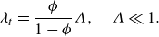 \begin{align}&\qquad \lambda _{t} = \frac {\phi }{1-\phi }\Lambda, \quad \Lambda \ll 1. \end{align}
As already highlighted at the end of § 2.3.1, based on the results reported in figures 2(a) and 2(b), it is observed that $\lambda _{\parallel, f}=\lambda _t$
, while
$\lambda _{\parallel, f}=\lambda _t$
, while $\lambda _{\perp, f}$
remains a constant value proportional to them in both asymptotic ranges. As shown in figure 2(d), the ratio
$\lambda _{\perp, f}$
remains a constant value proportional to them in both asymptotic ranges. As shown in figure 2(d), the ratio $\lambda _{\perp, f}/\lambda _t$
varies between 0.25 and 0.5 depending on
$\lambda _{\perp, f}/\lambda _t$
varies between 0.25 and 0.5 depending on $\phi$
and
$\phi$
and $\Lambda$
, consistent with
$\Lambda$
, consistent with $\lambda _{\parallel, f} = \lambda _t = 2\lambda _{\perp, f} = \ln (\sec (\phi \pi /2) )/\pi$
for
$\lambda _{\parallel, f} = \lambda _t = 2\lambda _{\perp, f} = \ln (\sec (\phi \pi /2) )/\pi$
for $\Lambda \gg 1$
, and
$\Lambda \gg 1$
, and $\lambda _{\parallel, f} = \lambda _t = 4\lambda _{\perp, f} = \phi \Lambda /(1-\phi )$
for
$\lambda _{\parallel, f} = \lambda _t = 4\lambda _{\perp, f} = \phi \Lambda /(1-\phi )$
for $\Lambda \ll 1$
.
$\Lambda \ll 1$
.
3.1.2. Velocity slip length
$\lambda _{\parallel, c}$
at a curved gas–liquid interface

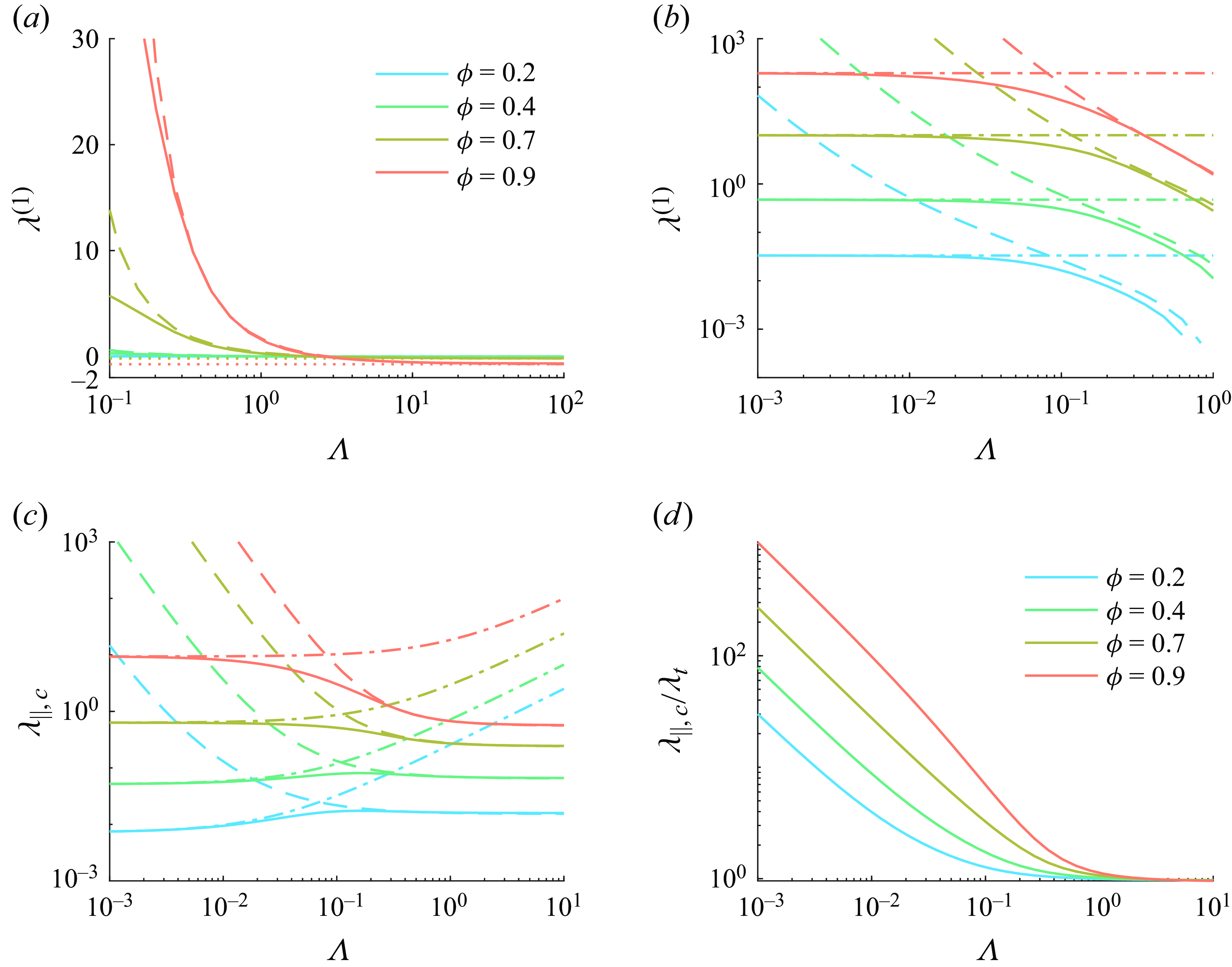
Figure 3. Slip lengths at a curved interface. (a–b) Variation of the first-order velocity slip length $\lambda ^{(1)}$
for different
$\lambda ^{(1)}$
for different $\Lambda$
, where a dotted line denotes (3.4), a dashed line (3.9) and a dot–dash line (3.10). (c) Total velocity slip length
$\Lambda$
, where a dotted line denotes (3.4), a dashed line (3.9) and a dot–dash line (3.10). (c) Total velocity slip length $\lambda _{\parallel, c}=\lambda ^{(0)}+\epsilon \lambda ^{(1)}$
versus
$\lambda _{\parallel, c}=\lambda ^{(0)}+\epsilon \lambda ^{(1)}$
versus $\Lambda$
, with a dashed line denoting (3.12) and a dot–dash line (3.11). (d) The ratio of the total velocity and temperature slip lengths,
$\Lambda$
, with a dashed line denoting (3.12) and a dot–dash line (3.11). (d) The ratio of the total velocity and temperature slip lengths, $\lambda _{\parallel, c}/\lambda _t$
, versus
$\lambda _{\parallel, c}/\lambda _t$
, versus $\Lambda$
.
$\Lambda$
.
We next consider the velocity slip length $\lambda _{\parallel, c}$
at a curved gas–liquid interface as a function of
$\lambda _{\parallel, c}$
at a curved gas–liquid interface as a function of $\Lambda$
and
$\Lambda$
and $\phi$
. The semilog and log–log results of the first-order slip length
$\phi$
. The semilog and log–log results of the first-order slip length $\lambda ^{(1)}$
, computed as described in § 2.3.2, are shown in figures 3(a) and 3(b), respectively. For different
$\lambda ^{(1)}$
, computed as described in § 2.3.2, are shown in figures 3(a) and 3(b), respectively. For different $\phi$
,
$\phi$
, $\lambda ^{(1)}$
exhibits two plateau intervals as
$\lambda ^{(1)}$
exhibits two plateau intervals as $\Lambda \ll 1$
and
$\Lambda \ll 1$
and $\Lambda \gg 1$
, with a decreasing trend as
$\Lambda \gg 1$
, with a decreasing trend as $\Lambda$
increases. Notably, when
$\Lambda$
increases. Notably, when $\Lambda \gtrsim 2$
,
$\Lambda \gtrsim 2$
, $\lambda ^{(1)}$
becomes negative. This occurs because the increased area for flow caused by the meniscus is negligible, while there is a reduced velocity gradient at the boundary
$\lambda ^{(1)}$
becomes negative. This occurs because the increased area for flow caused by the meniscus is negligible, while there is a reduced velocity gradient at the boundary $y=0$
due to the meniscus.
$y=0$
due to the meniscus.
The asymptotic solution of the first-order slip length $\lambda ^{(1)}$
, with
$\lambda ^{(1)}$
, with ${O}(\Lambda ^{-1})$
error, has already been proposed (Sbragaglia & Prosperetti Reference Sbragaglia and Prosperetti2007; Kirk et al. Reference Kirk, Hodes and Papageorgiou2017),
${O}(\Lambda ^{-1})$
error, has already been proposed (Sbragaglia & Prosperetti Reference Sbragaglia and Prosperetti2007; Kirk et al. Reference Kirk, Hodes and Papageorgiou2017),
 \begin{equation} \lambda _{\|}^{(1)}= -\phi ^3\int _{0}^{1} \frac {\left [1-\cos \left (\phi \pi s\right )\right ]\left (1-s^2\right )}{\cos \left (\phi \pi s\right )-\cos \left (\phi \pi \right )}\textrm{d}s + {O}(\Lambda ^{-1}), \quad \Lambda \gg 1, \end{equation}
which only accounts for the changed velocity profile and neglects effects of increased flow rate associated with an expanded area, corresponding to the slip length
 \begin{equation} \lambda _{\|, c}=\ln (\sec (\phi \pi / 2)) / \pi -\epsilon \phi ^3 \mathcal{F}(\phi ),\quad \Lambda \gg 1; \end{equation}
the function $\mathcal{F}(\phi )$
is defined shortly. Based on (2.39b
) in the limit of
$\mathcal{F}(\phi )$
is defined shortly. Based on (2.39b
) in the limit of $\Lambda \gg 1$
, we can give the flow rate
$\Lambda \gg 1$
, we can give the flow rate $Q^{(1)}$
as
$Q^{(1)}$
as
 \begin{equation} Q^{(1)}= -\frac {\phi ^3\Lambda ^2l}{4} \mathcal{F}(\phi ) +\pi \phi ^4\Lambda l^2 \mathcal{G}(\phi ),\quad \Lambda \gg 1, \end{equation}
where $\mathcal{F(\phi )}$
and
$\mathcal{F(\phi )}$
and $\mathcal{G(\phi )}$
are
$\mathcal{G(\phi )}$
are
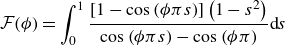 \begin{equation} \mathcal{F}(\phi )=\int _{0}^{1} \frac {\left [1-\cos \left (\phi \pi s\right )\right ]\left (1-s^2\right )}{\cos \left (\phi \pi s\right )-\cos \left (\phi \pi \right )}\textrm{d}s \end{equation}
and
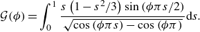 \begin{equation} \mathcal{G}(\phi )=\int _{0}^{1} \frac {s\left (1-s^2/3\right )\sin \left (\phi \pi s/2\right )}{\sqrt {\cos \left (\phi \pi s\right )-\cos \left (\phi \pi \right )}}\textrm{d}s. \end{equation}
These two integral functions can be referred to in previous work (Sneddon Reference Sneddon1966; Sbragaglia & Prosperetti Reference Sbragaglia and Prosperetti2007). Hence, a modified asymptotic solution of $\lambda _{\parallel }^{(1)}$
for
$\lambda _{\parallel }^{(1)}$
for $\Lambda \gtrsim 0.2$
is proposed as
$\Lambda \gtrsim 0.2$
is proposed as
 \begin{equation} \lambda _{\|}^{(1)}=\left (-\phi ^3 \mathcal{F}(\phi ) +\frac {4}{\Lambda }\phi ^4 \mathcal{G}(\phi )\right )\left (1+ \frac {1}{4\Lambda \pi } \ln \left (\sec \left (\frac {\phi \pi }{2}\right )\right )\right )^2,\quad \Lambda \gtrsim 0.2. \end{equation}
In the limit of $\Lambda \ll 1$
, an asymptotic solution can be derived by substituting
$\Lambda \ll 1$
, an asymptotic solution can be derived by substituting $\lambda _{\parallel }^{(0)}=l\phi \Lambda /(1-\phi )$
and
$\lambda _{\parallel }^{(0)}=l\phi \Lambda /(1-\phi )$
and $Q^{(1)} = 2\phi ^3\Lambda ^2l/3$
into the second term of (2.40), leading to
$Q^{(1)} = 2\phi ^3\Lambda ^2l/3$
into the second term of (2.40), leading to
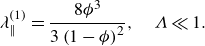 \begin{equation} \lambda _{\parallel }^{(1)}=\frac {8\phi ^3}{3\left (1-\phi \right )^2},\quad \Lambda \ll 1. \end{equation}
As depicted in figures 3(a) and 3(b), the asymptotic solutions (3.4) and (3.10) for the plateaus can accurately predict the first-order velocity slip length $\lambda ^{(1)}$
for different
$\lambda ^{(1)}$
for different $\phi$
. However, their applicability is limited (
$\phi$
. However, their applicability is limited ( $\Lambda \lesssim 0.01$
or
$\Lambda \lesssim 0.01$
or $\Lambda \gtrsim 10^2$
), while the newly proposed modified asymptotic solution (3.9) can accurately predict the first-order velocity slip for
$\Lambda \gtrsim 10^2$
), while the newly proposed modified asymptotic solution (3.9) can accurately predict the first-order velocity slip for $\Lambda \gtrsim 0.2$
.
$\Lambda \gtrsim 0.2$
.
Based on the velocity slip length of zeroth-order $\lambda ^{(0)}$
and first-order
$\lambda ^{(0)}$
and first-order $\lambda ^{(1)}$
, the slip length for a curved liquid surface,
$\lambda ^{(1)}$
, the slip length for a curved liquid surface, $\lambda _{\parallel, c}$
, can be finally obtained according to the equation
$\lambda _{\parallel, c}$
, can be finally obtained according to the equation $\lambda _{\parallel, c}=\lambda ^{(0)}+\epsilon \lambda ^{(1)}$
, which is plotted for different
$\lambda _{\parallel, c}=\lambda ^{(0)}+\epsilon \lambda ^{(1)}$
, which is plotted for different $\phi$
as solid lines in figure 3(c). The corresponding asymptotic solutions of
$\phi$
as solid lines in figure 3(c). The corresponding asymptotic solutions of $\lambda _{\parallel, c}$
are also drawn as dot–dash and dashed lines, corresponding, respectively, to the equations
$\lambda _{\parallel, c}$
are also drawn as dot–dash and dashed lines, corresponding, respectively, to the equations
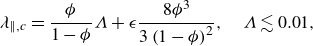 \begin{equation} \lambda _{\parallel, c}=\frac {\phi }{1-\phi }\Lambda + \epsilon \frac {8\phi ^3}{3\left (1-\phi \right )^2},\quad \Lambda \lesssim 0.01, \end{equation}
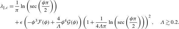 \begin{align} \lambda _{\parallel, c}&=\frac {1}{\pi } \ln \left (\sec \left (\frac {\phi \pi }{2}\right )\right )\nonumber\\&\quad + \epsilon \left (-\phi ^3 \mathcal{F}(\phi ) +\frac {4}{\Lambda }\phi ^4 \mathcal{G}(\phi )\right )\left (1+ \frac {1}{4\Lambda \pi } \ln \left (\sec \left (\frac {\phi \pi }{2}\right )\right )\right )^2,\quad \Lambda \gtrsim 0.2. \end{align}
The presence of a meniscus leads to a constant value of $\lambda _{\parallel, c}$
when
$\lambda _{\parallel, c}$
when $\Lambda \ll 1$
. Hence, the results for
$\Lambda \ll 1$
. Hence, the results for $\lambda _{\parallel, c}/\lambda _t$
indicate potentially large values up to
$\lambda _{\parallel, c}/\lambda _t$
indicate potentially large values up to ${O}(10^2)$
compared with
${O}(10^2)$
compared with $\lambda _{\parallel, f}/\lambda _t=1$
, when
$\lambda _{\parallel, f}/\lambda _t=1$
, when $\Lambda \ll 1$
for arbitrary
$\Lambda \ll 1$
for arbitrary $\phi$
, as plotted in figure 3(d). The results imply that the existence of a meniscus may enhance CCM due to a significant effect of velocity slip compared with thermal slip.
$\phi$
, as plotted in figure 3(d). The results imply that the existence of a meniscus may enhance CCM due to a significant effect of velocity slip compared with thermal slip.
The asymptotic solutions obtained in this section (§ 3.1) are summarised in table 1 for convenient comparison. The effects of gas–liquid fraction $\phi$
, aspect ratio
$\phi$
, aspect ratio $\Lambda$
and the presence of a meniscus on the velocity slip length
$\Lambda$
and the presence of a meniscus on the velocity slip length $\lambda$
and temperature slip length
$\lambda$
and temperature slip length $\lambda _t$
can be summarized as follows. (i) Increasing
$\lambda _t$
can be summarized as follows. (i) Increasing $\phi$
always leads to an increase in both
$\phi$
always leads to an increase in both $\lambda$
and
$\lambda$
and $\lambda _t$
, as the proportion of the gas–liquid interfaces
$\lambda _t$
, as the proportion of the gas–liquid interfaces $\phi$
that allows slip increases. (ii) In the absence of deformation of the meniscus, when
$\phi$
that allows slip increases. (ii) In the absence of deformation of the meniscus, when $\Lambda \gg 1$
, the slip lengths become independent of
$\Lambda \gg 1$
, the slip lengths become independent of $\Lambda$
because for such aspect ratios there is no change on the local velocity or temperature distribution near the gas–liquid interface (figure 8
g–i); under such conditions, a no-slip top boundary is effectively equivalent to a free-shear or thermally insulating one. In contrast, when
$\Lambda$
because for such aspect ratios there is no change on the local velocity or temperature distribution near the gas–liquid interface (figure 8
g–i); under such conditions, a no-slip top boundary is effectively equivalent to a free-shear or thermally insulating one. In contrast, when $\Lambda \ll 1$
, the no-slip condition at the top boundary significantly affects the flow or thermal field near the gas–liquid interface (figure 8
a–f), causing both
$\Lambda \ll 1$
, the no-slip condition at the top boundary significantly affects the flow or thermal field near the gas–liquid interface (figure 8
a–f), causing both $\lambda$
and
$\lambda$
and $\lambda _t$
to decrease and approach zero as
$\lambda _t$
to decrease and approach zero as $\Lambda \to 0$
. (iii) When deformation of the meniscus is included, the temperature distribution is modified, but since the meniscus is assumed to be adiabatic, it does not contribute to the net heat flux, and the effective temperature slip length
$\Lambda \to 0$
. (iii) When deformation of the meniscus is included, the temperature distribution is modified, but since the meniscus is assumed to be adiabatic, it does not contribute to the net heat flux, and the effective temperature slip length $\lambda _t$
remains unchanged. (iv) However, for velocity slip, the meniscus provides an additional flow area, and this contribution becomes more pronounced as
$\lambda _t$
remains unchanged. (iv) However, for velocity slip, the meniscus provides an additional flow area, and this contribution becomes more pronounced as $\Lambda$
decreases. Consequently,
$\Lambda$
decreases. Consequently, $\lambda$
does not vanish as
$\lambda$
does not vanish as $\Lambda \to 0$
but instead approaches a finite value that depends solely on
$\Lambda \to 0$
but instead approaches a finite value that depends solely on $\phi$
.
$\phi$
.
3.2. Characterizing constant-pressure CCM
We now use the main results of § 3.1 to calculate the melting rate. Recalling (2.52a
) with $\mathscr{c}=0$
, we observe that a constant dimensionless liquid film thickness
$\mathscr{c}=0$
, we observe that a constant dimensionless liquid film thickness $h=h^*/h^*_0$
can be determined due to a constant exerted pressure, yielding
$h=h^*/h^*_0$
can be determined due to a constant exerted pressure, yielding
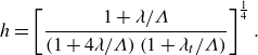 \begin{equation} h = \left [\frac {1+ \lambda /\Lambda }{\left (1+4 \lambda /\Lambda \right )\left (1+ \lambda _{t}/\Lambda \right )}\right ]^{\frac {1}{4}}. \end{equation}
Substitution of (3.13) into the definition of $\textrm{Nu}$
(2.53) leads to a prediction for the melting rate
$\textrm{Nu}$
(2.53) leads to a prediction for the melting rate
 \begin{equation} {\textrm{Nu}} = \left [\frac {1+4\lambda /\Lambda }{\left (1+ \lambda /\Lambda \right )\left (1+ \lambda _{t}/\Lambda \right )^3}\right ]^{\frac {1}{4}}. \end{equation}
Note that ${\textrm{Nu}} = 1$
represents the heat transfer performance of a smooth, unstructured surface (
${\textrm{Nu}} = 1$
represents the heat transfer performance of a smooth, unstructured surface ( $\lambda =\lambda _t=0$
). Therefore,
$\lambda =\lambda _t=0$
). Therefore, ${\textrm{Nu}} \gt 1$
indicates that the effects of velocity slip and temperature slip enhance heat transfer. Conversely,
${\textrm{Nu}} \gt 1$
indicates that the effects of velocity slip and temperature slip enhance heat transfer. Conversely, ${\textrm{Nu}} \lt 1$
implies a reduction in heat transfer.
${\textrm{Nu}} \lt 1$
implies a reduction in heat transfer.
3.2.1. Flat liquid–gas interface
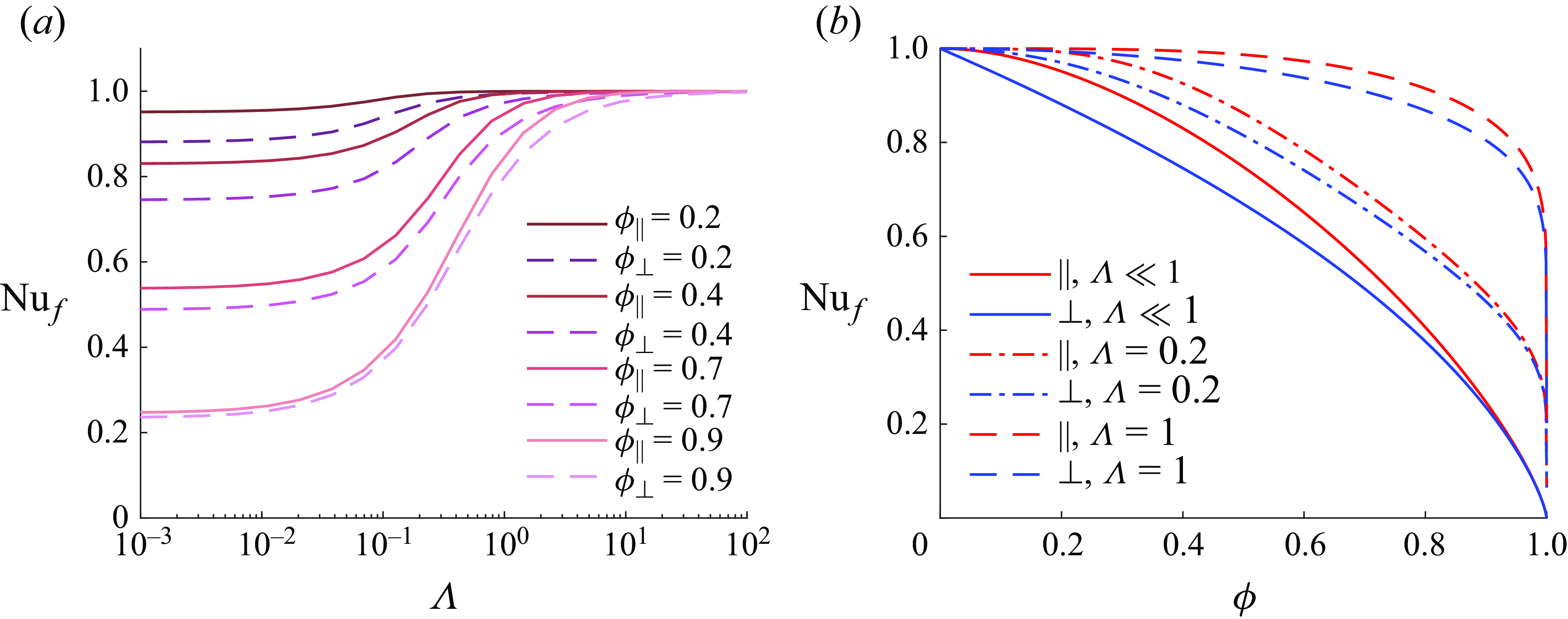
Figure 4. Variation of $\textrm{Nu}_f$
along with (a) aspect ratio
$\textrm{Nu}_f$
along with (a) aspect ratio $\Lambda$
by numerical results and (b) liquid–gas fraction
$\Lambda$
by numerical results and (b) liquid–gas fraction $\phi$
by asymptotic formula for flat gas–liquid interface. Here
$\phi$
by asymptotic formula for flat gas–liquid interface. Here $\parallel$
and
$\parallel$
and $\perp$
represent longitudinal and transverse grooves, respectively.
$\perp$
represent longitudinal and transverse grooves, respectively.
Substituting the numerical results of $\lambda _{\parallel, f}$
and
$\lambda _{\parallel, f}$
and $\lambda _{\perp, f}$
, respectively, obtained from § 2.2.1 and Appendix F into (3.14) yields the results of
$\lambda _{\perp, f}$
, respectively, obtained from § 2.2.1 and Appendix F into (3.14) yields the results of $\textrm{Nu}_f$
versus
$\textrm{Nu}_f$
versus $\Lambda$
for a flat interface shown in figure 4(a). For both longitudinal and transverse groove structures, the existence of slip always reduces heat transfer. When
$\Lambda$
for a flat interface shown in figure 4(a). For both longitudinal and transverse groove structures, the existence of slip always reduces heat transfer. When $\Lambda \gg 1$
,
$\Lambda \gg 1$
, $\textrm{Nu}_f$
asymptotically equals 1 due to negligible slip effect. For the case of
$\textrm{Nu}_f$
asymptotically equals 1 due to negligible slip effect. For the case of $\Lambda \ll 1$
,
$\Lambda \ll 1$
, $\textrm{Nu}_f$
decreases and then asymptotically equals a constant value for either the longitudinal or transverse grooves. It is obvious that
$\textrm{Nu}_f$
decreases and then asymptotically equals a constant value for either the longitudinal or transverse grooves. It is obvious that $\textrm{Nu}_{\parallel, f} \gt \textrm{Nu}_{\perp, f}$
is valid for any
$\textrm{Nu}_{\parallel, f} \gt \textrm{Nu}_{\perp, f}$
is valid for any $\phi$
. Therefore, we can determine that
$\phi$
. Therefore, we can determine that $\textrm{Nu}_f$
varies only as a function of
$\textrm{Nu}_f$
varies only as a function of $\phi$
within the asymptotic region (
$\phi$
within the asymptotic region ( $\Lambda \ll 1$
as indicated in figure 2). By substituting the asymptotic solutions from § 3.1.1, we find
$\Lambda \ll 1$
as indicated in figure 2). By substituting the asymptotic solutions from § 3.1.1, we find
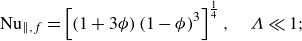 \begin{align}& \textrm{Nu}_{\parallel, f}=\left [\left (1+3\phi \right )\left (1-\phi \right )^3\right ]^{\frac {1}{4}}, \quad \Lambda \ll 1; \end{align}
 \begin{align}&\quad\,\, \textrm{Nu}_{\perp, f}=\left [\frac {4\left (1-\phi \right )^3}{4-3\phi }\right ]^{\frac {1}{4}},\quad \Lambda \ll 1, \end{align}
which are plotted in figure 4(b). All curves generally show a decreasing trend of $\textrm{Nu}$
as
$\textrm{Nu}$
as $\phi$
increases. For
$\phi$
increases. For $\Lambda \ll 1$
, the parallel and perpendicular values of
$\Lambda \ll 1$
, the parallel and perpendicular values of $\textrm{Nu}$
start at 1 and decrease with increasing liquid–gas fraction
$\textrm{Nu}$
start at 1 and decrease with increasing liquid–gas fraction $\phi$
. For larger values of
$\phi$
. For larger values of $\Lambda =$
0.2 and 1, the curves for both
$\Lambda =$
0.2 and 1, the curves for both $\textrm{Nu}_{\parallel, f}$
and
$\textrm{Nu}_{\parallel, f}$
and $\textrm{Nu}_{\perp, f}$
exhibit more pronounced decreases and diverge more significantly as
$\textrm{Nu}_{\perp, f}$
exhibit more pronounced decreases and diverge more significantly as $\phi$
approaches 1. The curves suggest that the parameter
$\phi$
approaches 1. The curves suggest that the parameter $\Lambda$
significantly impacts
$\Lambda$
significantly impacts $\textrm{Nu}_f$
, with higher values of
$\textrm{Nu}_f$
, with higher values of $\Lambda$
leading to more rapid decreases in
$\Lambda$
leading to more rapid decreases in $\textrm{Nu}_f$
.
$\textrm{Nu}_f$
.
3.2.2. A curved liquid–gas interface on longitudinal grooves
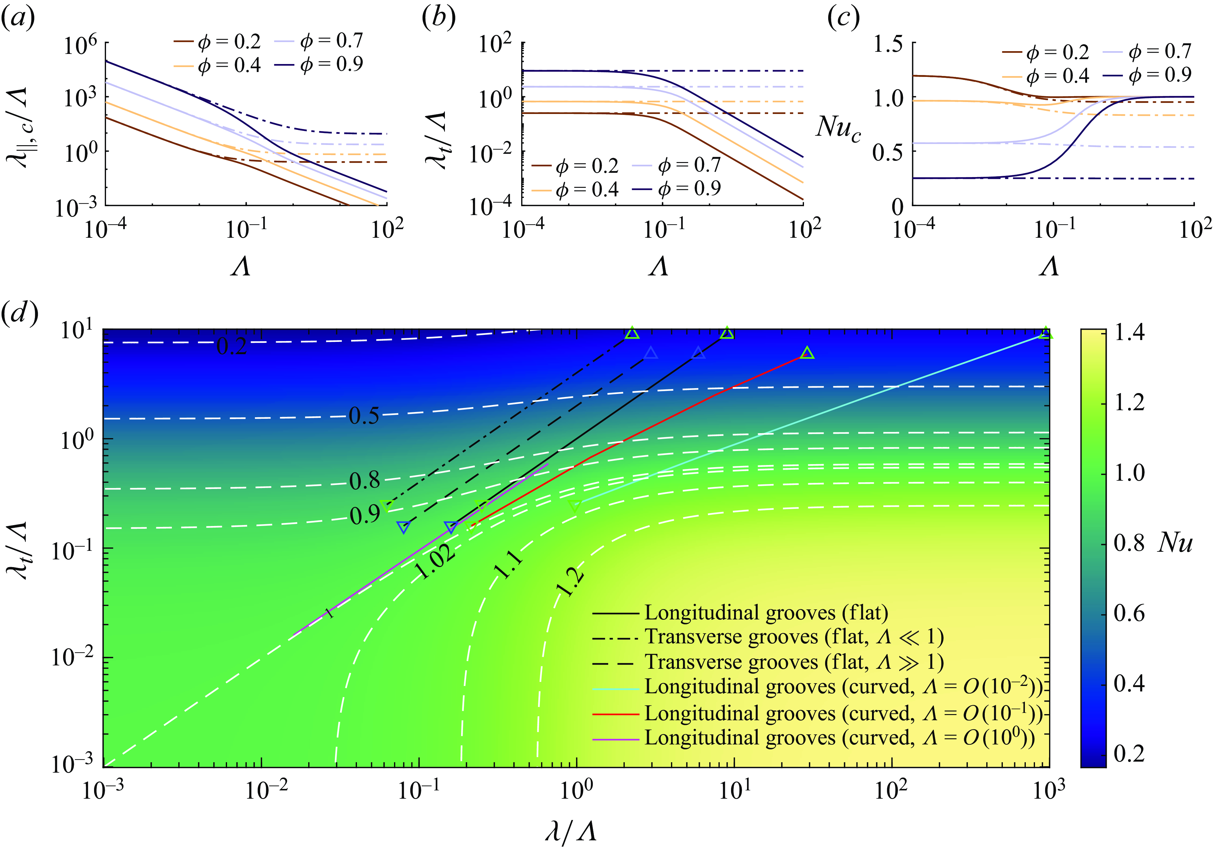
Figure 5. Variation of (a) $\lambda /\Lambda$
and (b)
$\lambda /\Lambda$
and (b) $\lambda _t/\Lambda$
versus
$\lambda _t/\Lambda$
versus $\Lambda$
, where solid lines represent numerical results and dot–dash lines represent asymptotic solutions listed in table 1. (c) Variation of
$\Lambda$
, where solid lines represent numerical results and dot–dash lines represent asymptotic solutions listed in table 1. (c) Variation of $\textrm{Nu}$
versus
$\textrm{Nu}$
versus $\Lambda$
for curved gas–liquid interface, dot–dash lines are asymptotic solutions (3.17). (d) Map of
$\Lambda$
for curved gas–liquid interface, dot–dash lines are asymptotic solutions (3.17). (d) Map of $\textrm{Nu}$
at the various combinations of
$\textrm{Nu}$
at the various combinations of $\Lambda$
,
$\Lambda$
, $\phi$
and transverse/longitudinal surface structures for constant-pressure mode. Symbols denote
$\phi$
and transverse/longitudinal surface structures for constant-pressure mode. Symbols denote ![]() ,
, $\phi =0.2$
and
$\phi =0.2$
and $\Lambda \gg 1$
;
$\Lambda \gg 1$
; ![]() ,
, $\phi =0.9$
and
$\phi =0.9$
and $\Lambda \gg 1$
;
$\Lambda \gg 1$
; ![]() ,
, $\phi =0.2$
and
$\phi =0.2$
and $\Lambda \ll 1$
;
$\Lambda \ll 1$
; ![]() ,
, $\phi =0.9$
and
$\phi =0.9$
and $\Lambda \ll 1$
.
$\Lambda \ll 1$
.
For a curved liquid–gas interface on longitudinal grooves, first we observe that $\lambda _{\parallel, c}/\Lambda$
and
$\lambda _{\parallel, c}/\Lambda$
and $\lambda _t/\Lambda$
can be considered as the functions of
$\lambda _t/\Lambda$
can be considered as the functions of $\Lambda$
as shown in figures 5(a) and 5(b), respectively. Similarly, by substituting the numerical solutions for
$\Lambda$
as shown in figures 5(a) and 5(b), respectively. Similarly, by substituting the numerical solutions for $\lambda _{\parallel, c}$
and
$\lambda _{\parallel, c}$
and $\lambda _{t}$
into (3.14), we can obtain the numerical results of
$\lambda _{t}$
into (3.14), we can obtain the numerical results of $\textrm{Nu}_c$
for considering a meniscus on longitudinal grooves, as plotted in figure 5(c). Compared with the flat interface,
$\textrm{Nu}_c$
for considering a meniscus on longitudinal grooves, as plotted in figure 5(c). Compared with the flat interface, $\textrm{Nu}_c$
is also close to 1 for
$\textrm{Nu}_c$
is also close to 1 for $\Lambda \gg 1$
. However, as
$\Lambda \gg 1$
. However, as $\Lambda \to 0$
, there exists a critical
$\Lambda \to 0$
, there exists a critical $\phi$
at which
$\phi$
at which $\textrm{Nu}_c$
can be larger than 1 and heat transfer is enhanced. By substituting the asymptotic slip length solution (3.11) at
$\textrm{Nu}_c$
can be larger than 1 and heat transfer is enhanced. By substituting the asymptotic slip length solution (3.11) at $\Lambda \ll 1$
into (3.14), we find
$\Lambda \ll 1$
into (3.14), we find
 \begin{equation} \textrm{Nu}_{c}=\left (\frac {(1-\phi )^3\left (3 \Lambda \left (1+2 \phi -3 \phi ^2\right )+8 \phi ^2 \sin {\theta }\right )}{3 \Lambda (1-\phi )+2 \phi ^2 \sin {\theta }}\right )^{\frac {1}{4}} \overset {\Lambda \rightarrow 0}{=}\left [4(1-\phi )^{3}\right ]^{\frac {1}{4}}, \end{equation}
which is plotted as dot–dash lines for different $\phi$
in figure 5(c). Then, by setting
$\phi$
in figure 5(c). Then, by setting ${\textrm{Nu}}_c =1$
, we can obtain the critical fraction
${\textrm{Nu}}_c =1$
, we can obtain the critical fraction $\phi _{cr} = 1-2^{-2/3} \approx 0.37$
. Therefore, we infer that when
$\phi _{cr} = 1-2^{-2/3} \approx 0.37$
. Therefore, we infer that when $\phi \gt 0.37$
, heat transfer will be reduced regardless of the value of
$\phi \gt 0.37$
, heat transfer will be reduced regardless of the value of $\Lambda$
. However, when
$\Lambda$
. However, when $\phi \lt 0.37$
, heat transfer can be enhanced to accelerate melting, with
$\phi \lt 0.37$
, heat transfer can be enhanced to accelerate melting, with $\textrm{Nu}_c$
approaching a constant value of
$\textrm{Nu}_c$
approaching a constant value of $4^{1/4}(1-\phi )^{3/4}$
as
$4^{1/4}(1-\phi )^{3/4}$
as $\Lambda$
decreases.
$\Lambda$
decreases.
In order to visually compare the effects of surface structure, a meniscus, aspect ratio ( $\Lambda$
) and gas–liquid ratio (
$\Lambda$
) and gas–liquid ratio ( $\phi$
) on
$\phi$
) on $\textrm{Nu}$
, a two-dimensional phase diagram is presented in figure 5(d). In this diagram, the contours correspond to varying
$\textrm{Nu}$
, a two-dimensional phase diagram is presented in figure 5(d). In this diagram, the contours correspond to varying $\textrm{Nu}$
, with white dashed lines representing
$\textrm{Nu}$
, with white dashed lines representing $\textrm{Nu}$
isoclines and other lines indicating results derived from asymptotic solutions. It can be observed that for a flat interface,
$\textrm{Nu}$
isoclines and other lines indicating results derived from asymptotic solutions. It can be observed that for a flat interface, ${\textrm{Nu}}\lt 1$
always remains for surfaces with transverse groove structures, indicating a reduction in heat transfer effectiveness. In contrast, surfaces with longitudinal grooves maintain
${\textrm{Nu}}\lt 1$
always remains for surfaces with transverse groove structures, indicating a reduction in heat transfer effectiveness. In contrast, surfaces with longitudinal grooves maintain ${\textrm{Nu}} \rightarrow 1$
for small
${\textrm{Nu}} \rightarrow 1$
for small $\phi$
values, but
$\phi$
values, but $\textrm{Nu}$
decreases monotonically as
$\textrm{Nu}$
decreases monotonically as $\phi$
increases. When a meniscus (curved interface) is introduced,
$\phi$
increases. When a meniscus (curved interface) is introduced, ${\textrm{Nu}}\gt 1$
can be achieved for longitudinal grooves initially at small
${\textrm{Nu}}\gt 1$
can be achieved for longitudinal grooves initially at small $\phi$
and
$\phi$
and $\Lambda \lt 1$
, while
$\Lambda \lt 1$
, while $\textrm{Nu}$
shows a non-monotonic trend versus
$\textrm{Nu}$
shows a non-monotonic trend versus $\phi$
. The enhancement of
$\phi$
. The enhancement of $\textrm{Nu}$
at
$\textrm{Nu}$
at $\phi \lt 0.37$
is more pronounced as
$\phi \lt 0.37$
is more pronounced as $\Lambda$
decreases.
$\Lambda$
decreases.
Overall, under the condition of constant pressure, longitudinal grooves ( $\parallel$
) exhibit the best heat transfer performance among all surfaces. Furthermore, only with the presence of a meniscus and significant confinement effects (
$\parallel$
) exhibit the best heat transfer performance among all surfaces. Furthermore, only with the presence of a meniscus and significant confinement effects ( $\Lambda \ll 1$
), can one achieve an enhancement in heat transfer at an appropriate gas–liquid fraction (
$\Lambda \ll 1$
), can one achieve an enhancement in heat transfer at an appropriate gas–liquid fraction ( $\phi \lt 0.37$
).
$\phi \lt 0.37$
).
3.3. Gravity-driven CCM
In contrast with the constant pressure mode just discussed, when the PCM is supported only by hydrostatic pressure, i.e. the gravity-driven mode (i.e. $\mathscr{c}=1$
), the film thickness
$\mathscr{c}=1$
), the film thickness $h^*(t^*)$
changes in time due to the continuously decreasing size of the PCM solid.
$h^*(t^*)$
changes in time due to the continuously decreasing size of the PCM solid.
3.3.1. Numerical results of solid height
$H(\tau )$
and film thickness
$h(\tau )$


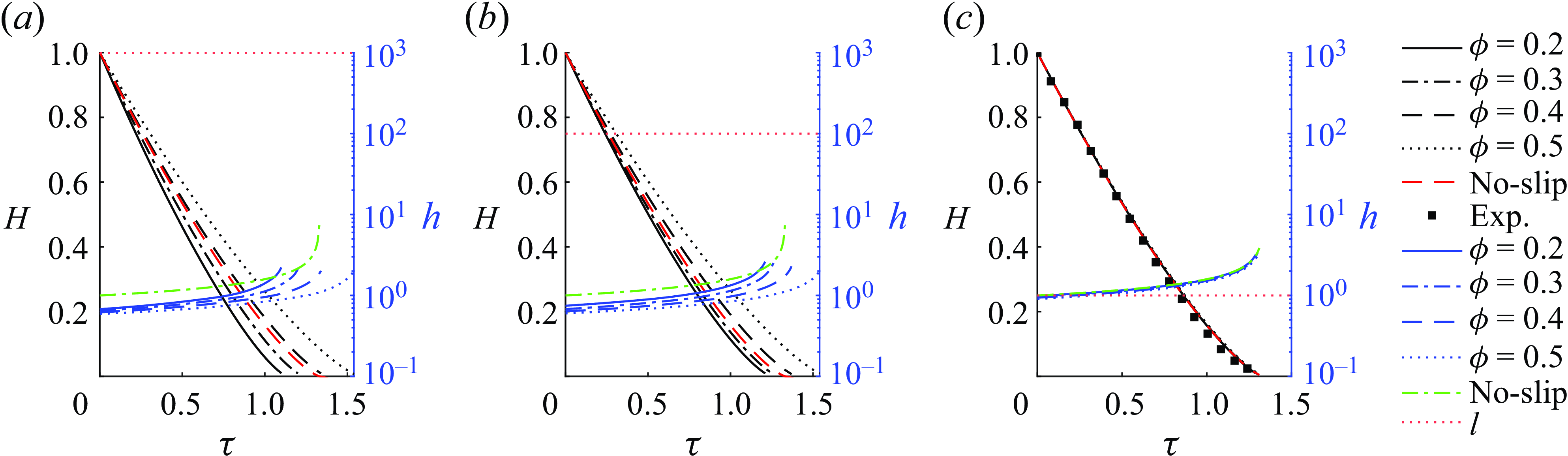
Figure 6. Variation of $H$
and
$H$
and $h$
versus
$h$
versus $\tau$
for different conditions of (a)
$\tau$
for different conditions of (a) $l=10^3$
, (b)
$l=10^3$
, (b) $l=10^2$
and (c)
$l=10^2$
and (c) $l=1$
. In all figures, the black line represents the remaining height
$l=1$
. In all figures, the black line represents the remaining height $H$
, the blue line represents the film thickness
$H$
, the blue line represents the film thickness $h$
, the red dotted line (
$h$
, the red dotted line (![]() ) represents the magnitude of
) represents the magnitude of $l$
, red dashed line (
$l$
, red dashed line (![]() ) and green dot–dash line(
) and green dot–dash line(![]() ) represent the no-slip solution of
) represent the no-slip solution of $H(\tau )$
(3.19a
) and
$H(\tau )$
(3.19a
) and $h(\tau )$
(3.19b
), respectively. Four values of
$h(\tau )$
(3.19b
), respectively. Four values of $\phi = \{0.1, 0.2, 0.3, 0.5\}$
are chosen for calculating each case. Experimental data (black squares) are replotted (Moallemi et al. Reference Moallemi, Webb and Viskanta1986) for comparison with the case
$\phi = \{0.1, 0.2, 0.3, 0.5\}$
are chosen for calculating each case. Experimental data (black squares) are replotted (Moallemi et al. Reference Moallemi, Webb and Viskanta1986) for comparison with the case $\phi = 0$
.
$\phi = 0$
.
Recalling (2.52a
) and (2.52b
) with $\mathscr{c}=1$
, we can rewrite them by using
$\mathscr{c}=1$
, we can rewrite them by using $h(\tau )=l\Lambda (\tau )$
from (2.1), yielding
$h(\tau )=l\Lambda (\tau )$
from (2.1), yielding
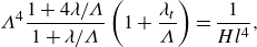 \begin{align}& \Lambda ^4\frac {1+4\lambda /\Lambda }{1+\lambda /\Lambda }\left (1+\frac {\lambda _{t}}{\Lambda }\right ) =\frac {1}{Hl^4}, \end{align}
 \begin{align}&\qquad \frac {{\textrm d}H}{{\textrm d}\tau }=-\frac {1}{l(\Lambda +\lambda _{t})} . \end{align}
This set of equations consists of a first-order ordinary differential equation and an algebraic equation, which can be numerically solved as detailed in Appendix G. For comparison, the analytical solution for a no-slip condition can be obtained by substituting $\lambda =\lambda _t=0$
into the above equations, yielding
$\lambda =\lambda _t=0$
into the above equations, yielding
 \begin{align}& H_{no-slip} = \left (1-\frac {3}{4}\tau \right )^{\frac {4}{3}}, \end{align}
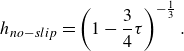 \begin{align}& h_{no-slip} = \left (1-\frac {3}{4}\tau \right )^{-\frac {1}{3}}. \end{align}
We estimated that the magnitude of $l$
ranges from
$l$
ranges from $10^{-1}$
to
$10^{-1}$
to $10^{3}$
, based on the representative values of the following dimensionless parameters:
$10^{3}$
, based on the representative values of the following dimensionless parameters: $\textrm{St} = 0.01-0.1$
and
$\textrm{St} = 0.01-0.1$
and ${A}^2 = 0.1-10$
, while
${A}^2 = 0.1-10$
, while $H_0^{*}$
varies from 0.01 m to 1 m and
$H_0^{*}$
varies from 0.01 m to 1 m and $l^{*}$
varies from 10
$l^{*}$
varies from 10 $\unicode{x03BC}$
m to 1 mm, with representative PCMs chosen as water and tetradecanol (Moallemi et al. Reference Moallemi, Webb and Viskanta1986; Feuillebois et al. Reference Feuillebois, Bazant and Vinogradova2009); by examining their thermophysical properties, liquid metals such as gallium or caesium are inadequate due to
$\unicode{x03BC}$
m to 1 mm, with representative PCMs chosen as water and tetradecanol (Moallemi et al. Reference Moallemi, Webb and Viskanta1986; Feuillebois et al. Reference Feuillebois, Bazant and Vinogradova2009); by examining their thermophysical properties, liquid metals such as gallium or caesium are inadequate due to $\textrm{Re}\mathscr{h}^2 \gtrsim 1$
. It is worth noting that
$\textrm{Re}\mathscr{h}^2 \gtrsim 1$
. It is worth noting that $l=l^* / h_0^*=l^* [ (T_w^*-T_m^* ) k_l^* L^{* 2} \mu ^* ]^{-1/4}(\mathcal{H}^* \rho _l^* p_c^*)^{1/4}$
includes the information of the heating condition, thermophysical properties of materials and sizes of grooves and the PCM solid, which are convenient indicators. Hence, varying
$l=l^* / h_0^*=l^* [ (T_w^*-T_m^* ) k_l^* L^{* 2} \mu ^* ]^{-1/4}(\mathcal{H}^* \rho _l^* p_c^*)^{1/4}$
includes the information of the heating condition, thermophysical properties of materials and sizes of grooves and the PCM solid, which are convenient indicators. Hence, varying $\phi$
and
$\phi$
and $l$
allows us to investigate the influences of various materials and surface structures.
$l$
allows us to investigate the influences of various materials and surface structures.
The representative results for $l \in \{10^{3}, 10^{2}, 10^{0}\}$
are drawn in figure 6 from figures 6(a) to 6(c), respectively. Since we have shown in § 3.2 that a flat interface (
$l \in \{10^{3}, 10^{2}, 10^{0}\}$
are drawn in figure 6 from figures 6(a) to 6(c), respectively. Since we have shown in § 3.2 that a flat interface ( $\parallel, f$
) always reduces the melting rate and similar results occur for the gravity-driven CCM here, only results considering a meniscus (
$\parallel, f$
) always reduces the melting rate and similar results occur for the gravity-driven CCM here, only results considering a meniscus ( $\parallel, c$
) are discussed in the following. For large
$\parallel, c$
) are discussed in the following. For large $l=10^3$
and
$l=10^3$
and $10^2$
, the results show that the melting rate
$10^2$
, the results show that the melting rate ${\textrm d}H/{\textrm d}\tau$
decreases with increased
${\textrm d}H/{\textrm d}\tau$
decreases with increased $\phi$
(black line) as illustrated in figures 6(a) and 6(b), though the film thickness
$\phi$
(black line) as illustrated in figures 6(a) and 6(b), though the film thickness $h$
also decreases along with larger
$h$
also decreases along with larger $\phi$
(blue line). This indicates that the temperature slip is more pronounced than the velocity slip. Compared with the case of no-slip (red dashed line),
$\phi$
(blue line). This indicates that the temperature slip is more pronounced than the velocity slip. Compared with the case of no-slip (red dashed line), $\phi \leqslant 0.3$
exhibits an accelerated melting rate due to slip, similar to the pressure-driven CCM in figure 5(c). When
$\phi \leqslant 0.3$
exhibits an accelerated melting rate due to slip, similar to the pressure-driven CCM in figure 5(c). When $l=1$
in figure 6(c), it can be demonstrated that all slip cases gradually approach those of no-slip (figure 6
d and 6
e). Although no experimental data are currently available to validate the model predictions of
$l=1$
in figure 6(c), it can be demonstrated that all slip cases gradually approach those of no-slip (figure 6
d and 6
e). Although no experimental data are currently available to validate the model predictions of $H(\tau )$
or
$H(\tau )$
or $h(\tau )$
under varying gas–liquid fraction
$h(\tau )$
under varying gas–liquid fraction $\phi$
and structure parameter
$\phi$
and structure parameter $l$
, experimental data for the limiting case of
$l$
, experimental data for the limiting case of $\phi = 0$
were reported in two-dimensional rectangular CCMs by Moallemi et al. (Reference Moallemi, Webb and Viskanta1986), allowing for direct comparison. As shown in figure 6(c), the model prediction agrees well with the experimental results, confirming the validity of the limiting solution (i.e. the no-slip case) presented in this study.
$\phi = 0$
were reported in two-dimensional rectangular CCMs by Moallemi et al. (Reference Moallemi, Webb and Viskanta1986), allowing for direct comparison. As shown in figure 6(c), the model prediction agrees well with the experimental results, confirming the validity of the limiting solution (i.e. the no-slip case) presented in this study.
In general, an increase in the value of $\phi$
will invariably result in a reduction in the thickness of the liquid film
$\phi$
will invariably result in a reduction in the thickness of the liquid film $h$
. However, the melting rate is decreased due to the more pronounced effect of temperature slip. The potential for slip to accelerate the melting process depends on the specific combination of
$h$
. However, the melting rate is decreased due to the more pronounced effect of temperature slip. The potential for slip to accelerate the melting process depends on the specific combination of $l$
and
$l$
and $\phi$
. When
$\phi$
. When $l$
is sufficiently large (e.g.
$l$
is sufficiently large (e.g. $10^2$
or
$10^2$
or $10^3$
), even a modest increase in
$10^3$
), even a modest increase in $\phi$
can enhance heat transfer, thereby accelerating the melting process. Conversely, as
$\phi$
can enhance heat transfer, thereby accelerating the melting process. Conversely, as $l$
diminishes, the influence of slip decreases correspondingly, ultimately becoming negligible.
$l$
diminishes, the influence of slip decreases correspondingly, ultimately becoming negligible.
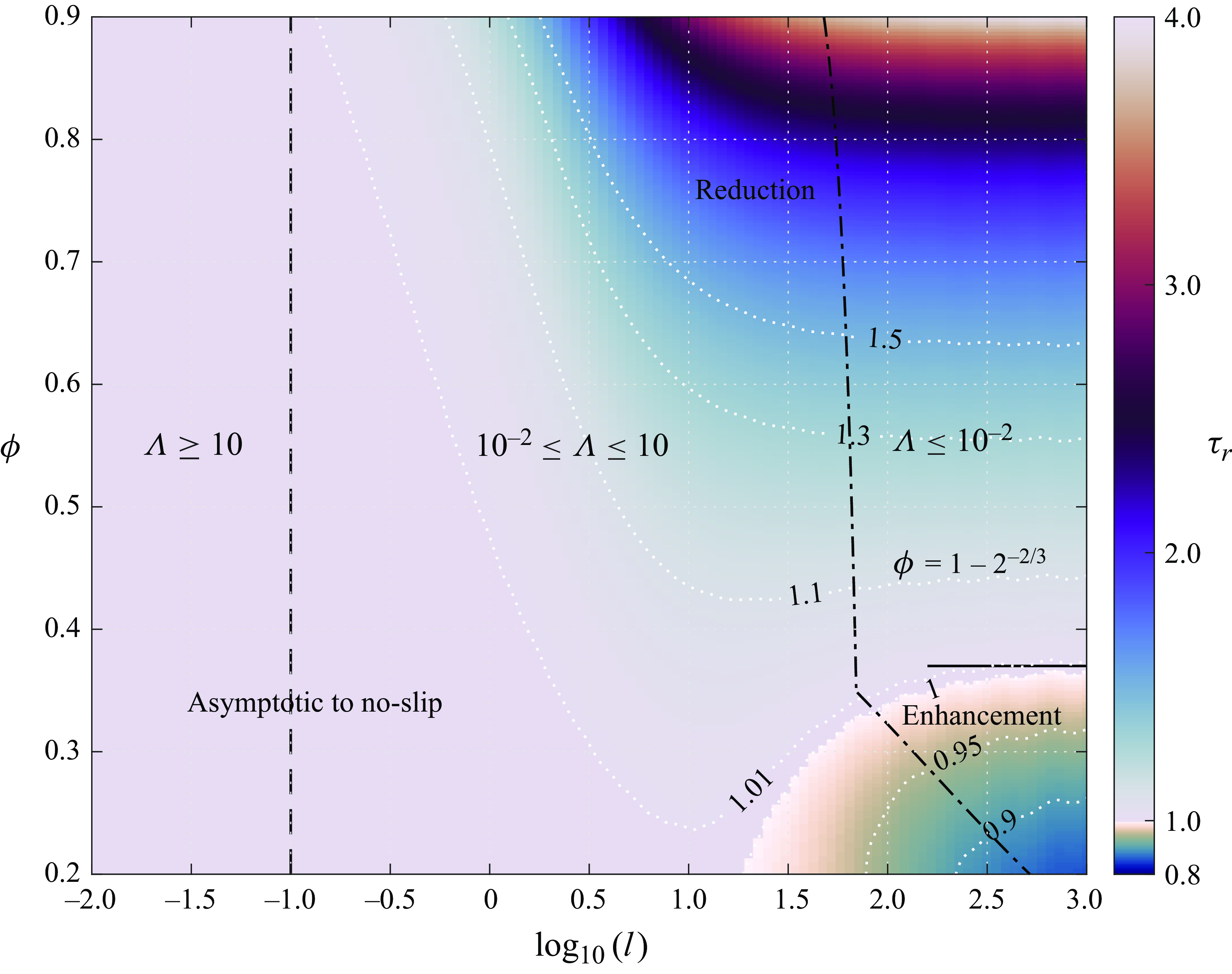
Figure 7. Phase diagram of melting time ratio $\tau _r$
of gravity-driven CCM with various combinations of gas–liquid fraction
$\tau _r$
of gravity-driven CCM with various combinations of gas–liquid fraction $\phi$
and periodic length
$\phi$
and periodic length $l$
on longitudinal grooves, where white dotted lines are contour lines for various
$l$
on longitudinal grooves, where white dotted lines are contour lines for various $\tau _r$
: black solid line,
$\tau _r$
: black solid line, $\phi = 1 - 2^{-2/3}$
; black dashed line, the asymptotic limit of
$\phi = 1 - 2^{-2/3}$
; black dashed line, the asymptotic limit of $l\lesssim 0.1$
for no-slip solutions (3.20); black dot–dash line, the asymptotic limits of (3.22a
) and (3.22b
) for solution (3.21).
$l\lesssim 0.1$
for no-slip solutions (3.20); black dot–dash line, the asymptotic limits of (3.22a
) and (3.22b
) for solution (3.21).
3.3.2. Phase diagram and asymptotic solution
To illustrate the effects of $\phi$
and
$\phi$
and $l$
, we selected 288 and 110 values from the ranges
$l$
, we selected 288 and 110 values from the ranges $\phi$
from 0.1–0.9 and
$\phi$
from 0.1–0.9 and $l$
from
$l$
from $10^{-2}$
–
$10^{-2}$
– $10^{3}$
, respectively. These values were used to construct the parameter matrix (log
$10^{3}$
, respectively. These values were used to construct the parameter matrix (log $_{10}l$
,
$_{10}l$
, $\phi$
), which was then substituted into the numerical solution calculations to obtain the total melting time
$\phi$
), which was then substituted into the numerical solution calculations to obtain the total melting time $\tau _{end}$
defined as
$\tau _{end}$
defined as $H(\tau _{end})=0$
for each case of (log
$H(\tau _{end})=0$
for each case of (log $_{10}l$
,
$_{10}l$
, $\phi$
). The resulting phase diagram is shown in figure 7, where the colour code represents
$\phi$
). The resulting phase diagram is shown in figure 7, where the colour code represents $\tau _r = \tau _{end}/\tau _{no-slip}=3\tau _{end} /4$
, meaning the melting time ratio of slip surface to no-slip surface.
$\tau _r = \tau _{end}/\tau _{no-slip}=3\tau _{end} /4$
, meaning the melting time ratio of slip surface to no-slip surface. $\tau _{no-slip}=4/3$
is obtained from (3.19a
), which corresponds to
$\tau _{no-slip}=4/3$
is obtained from (3.19a
), which corresponds to $\tau _r=1$
. Therefore,
$\tau _r=1$
. Therefore, $\tau _r \lt 1$
means heat transfer enhancement, while
$\tau _r \lt 1$
means heat transfer enhancement, while $\tau _r \gt 1$
means heat transfer reduction.
$\tau _r \gt 1$
means heat transfer reduction.
It can be observed that the region where enhancement effects can be achieved exists only in the lower right-hand corner of the phase diagram. The upper limit boundary is at $\phi = 1 - 2^{-2/3}$
, which is consistent with the conclusions drawn from the constant pressure CCM in § 3.2.2. The left-hand critical point of the region of heat transfer enhancement is approximately located at
$\phi = 1 - 2^{-2/3}$
, which is consistent with the conclusions drawn from the constant pressure CCM in § 3.2.2. The left-hand critical point of the region of heat transfer enhancement is approximately located at $(1.17, 0.125)$
. Unlike the region of heat transfer reduction, where
$(1.17, 0.125)$
. Unlike the region of heat transfer reduction, where $\tau _r$
changes monotonically with
$\tau _r$
changes monotonically with $\phi$
when
$\phi$
when $l$
is fixed, in the enhancement region,
$l$
is fixed, in the enhancement region, $\tau _r$
first decreases and then increases as
$\tau _r$
first decreases and then increases as $\phi$
decreases. This behaviour indicates that for a given
$\phi$
decreases. This behaviour indicates that for a given $l$
, there is always a specific value of
$l$
, there is always a specific value of $\phi$
that maximises heat transfer enhancement, which is plotted as yellow scatters in figure 7.
$\phi$
that maximises heat transfer enhancement, which is plotted as yellow scatters in figure 7.
Based on this phase diagram, we can further find two regions corresponding to two asymptotes (see details in Appendix H). One approximation is related to the no-slip solution for $\Lambda \geqslant 10$
, as
$\Lambda \geqslant 10$
, as
 \begin{equation} H(\tau ) = \left (1-\frac {3}{4}\tau \right )^{\frac {4}{3}}, \quad l \lesssim 0.1. \end{equation}
Another approximate solution satisfies $\Lambda \lesssim 0.01$
, as
$\Lambda \lesssim 0.01$
, as
 \begin{equation} H(\tau ;\phi )= \left (1-\frac {3\sqrt {2}}{4}\tau (1-\phi )^{\frac {3}{4}} \right )^{\frac {4}{3}}, \end{equation}
whose approximate limit conditions should be satisfied as
 \begin{align}&\qquad\quad 100\left (\frac {1-\phi }{4}\right )^{\frac {1}{5}} \lesssim l, \end{align}
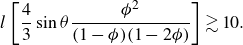 \begin{align}& l\left [{\frac {4}{3}\sin \theta \frac {\phi ^2}{(1-\phi )(1-2\phi )}}\right ] \gtrsim 10. \end{align}
Therefore, the upper right-hand region enclosed by the two dash–dotted lines in figure 7 represents the parameter range where asymptotic solution (3.21) is valid.
Comparison of numerical and asymptotic results from $l = 1-10^3$
are conducted in Appendix H. It shows a good agreement with predictions in the phase diagram by selecting
$l = 1-10^3$
are conducted in Appendix H. It shows a good agreement with predictions in the phase diagram by selecting $\phi =\{0.1,0.2,0.3,0.4,0.5,0.6\}$
for cases.
$\phi =\{0.1,0.2,0.3,0.4,0.5,0.6\}$
for cases.
4. Conclusions
In this work, we established a theoretical framework to investigate the dynamics of CCM on gas-trapped hydrophobic surfaces, with a particular focus on the effects of liquid film confinement and the meniscus at the gas–liquid interface. Utilizing dual-series and perturbation methods under the assumption of small meniscus deflections, we obtained numerical results for the velocity slip length $\lambda$
and temperature slip length
$\lambda$
and temperature slip length $\lambda _t$
across various aspect ratios
$\lambda _t$
across various aspect ratios $\Lambda$
and gas fraction
$\Lambda$
and gas fraction $\phi$
, representative of the liquid film thickness
$\phi$
, representative of the liquid film thickness $h$
relative to the period
$h$
relative to the period $l$
of the microstructure. For
$l$
of the microstructure. For $\Lambda \gg 1$
, the scaling laws are
$\Lambda \gg 1$
, the scaling laws are $\lambda _{\parallel, f} = \lambda _t = 2\lambda _{\perp, f} = \ln (\sec (\phi \pi /2) )/\pi$
, while for
$\lambda _{\parallel, f} = \lambda _t = 2\lambda _{\perp, f} = \ln (\sec (\phi \pi /2) )/\pi$
, while for $\Lambda \ll 1$
, they are
$\Lambda \ll 1$
, they are $\lambda _{\parallel, f} = \lambda _t = 4\lambda _{\perp, f} = \phi \Lambda /(1-\phi )$
, where
$\lambda _{\parallel, f} = \lambda _t = 4\lambda _{\perp, f} = \phi \Lambda /(1-\phi )$
, where $f$
,
$f$
, $\parallel$
and
$\parallel$
and $\perp$
denote a flat interface, longitudinal grooves and transverse grooves, respectively. Accounting for the meniscus at the gas–liquid interface, the velocity slip length changes to (3.5) and (3.11), showing a slight decrease for
$\perp$
denote a flat interface, longitudinal grooves and transverse grooves, respectively. Accounting for the meniscus at the gas–liquid interface, the velocity slip length changes to (3.5) and (3.11), showing a slight decrease for $\Lambda \gg 1$
and a significant increase for
$\Lambda \gg 1$
and a significant increase for $\Lambda \ll 1$
compared with the flat interface. This behaviour results from the larger area fraction and pronounced slip effects induced by the meniscus at
$\Lambda \ll 1$
compared with the flat interface. This behaviour results from the larger area fraction and pronounced slip effects induced by the meniscus at $\Lambda \ll 1$
, whereas at
$\Lambda \ll 1$
, whereas at $\Lambda \gg 1$
, the meniscus contributes negligible additional area, and the velocity gradient is reduced at the bottom. Additionally, a modified asymptotic solution for
$\Lambda \gg 1$
, the meniscus contributes negligible additional area, and the velocity gradient is reduced at the bottom. Additionally, a modified asymptotic solution for $\lambda _{\parallel, c}$
(3.12) is proposed, which is broadly applicable in the range
$\lambda _{\parallel, c}$
(3.12) is proposed, which is broadly applicable in the range $\Lambda \gtrsim 0.2$
.
$\Lambda \gtrsim 0.2$
.
For constant-pressure CCM, the dimensionless film thickness $h$
remains constant for a specific pressure
$h$
remains constant for a specific pressure $\mathcal{P}$
and both slip lengths,
$\mathcal{P}$
and both slip lengths, $\lambda$
and
$\lambda$
and $\lambda _t$
, lead to a slip-effective
$\lambda _t$
, lead to a slip-effective $\textrm{Nu}$
that determines whether heat transfer is enhanced (
$\textrm{Nu}$
that determines whether heat transfer is enhanced ( ${\textrm{Nu}} \gt 1$
) or decreased (
${\textrm{Nu}} \gt 1$
) or decreased ( ${\textrm{Nu}} \lt 1$
). When the gas–liquid interface is flat, we found that transverse grooves surfaces always deteriorate heat transfer regardless of
${\textrm{Nu}} \lt 1$
). When the gas–liquid interface is flat, we found that transverse grooves surfaces always deteriorate heat transfer regardless of $\Lambda$
and
$\Lambda$
and $\phi$
, while longitudinal grooves exhibit behaviour identical to a smooth surface at small
$\phi$
, while longitudinal grooves exhibit behaviour identical to a smooth surface at small $\phi$
but show deteriorated performance at large
$\phi$
but show deteriorated performance at large $\phi$
. In the presence of a meniscus at the gas–liquid interface, we observed an enhanced melting rate when
$\phi$
. In the presence of a meniscus at the gas–liquid interface, we observed an enhanced melting rate when $\Lambda \lesssim 0.1$
and
$\Lambda \lesssim 0.1$
and $\phi \lt 1-\sqrt [3]{2}/2 \approx 0.37$
. It is important to note that
$\phi \lt 1-\sqrt [3]{2}/2 \approx 0.37$
. It is important to note that $\textrm{Nu}$
does not vary monotonically with
$\textrm{Nu}$
does not vary monotonically with $\phi$
; instead, maximum values of
$\phi$
; instead, maximum values of $\textrm{Nu}$
occur under specific conditions within the range
$\textrm{Nu}$
occur under specific conditions within the range $\phi \lt 0.37$
seen in figure 5(c).
$\phi \lt 0.37$
seen in figure 5(c).
In gravity-driven CCM, the film thickness $h$
increases monotonically in time. Slip effects have a minor influence on
$h$
increases monotonically in time. Slip effects have a minor influence on $h$
and become negligible when
$h$
and become negligible when $\Lambda \gtrsim 10$
or when there is a combination of small
$\Lambda \gtrsim 10$
or when there is a combination of small $\phi$
and
$\phi$
and $\Lambda \sim 10^{-1} $
–
$\Lambda \sim 10^{-1} $
– $10$
. Conversely, significant slip effects are observed for smaller
$10$
. Conversely, significant slip effects are observed for smaller $\Lambda$
, particularly for
$\Lambda$
, particularly for $\Lambda \lesssim 10^{-2}$
. We developed a two-dimensional phase diagram based on
$\Lambda \lesssim 10^{-2}$
. We developed a two-dimensional phase diagram based on $(\log _{10} l, \phi )$
to identify regions of enhancement, reduction, or negligible impact of the gas–liquid boundaries (the generator of slip) relative to the no-slip case. Additionally, we derived asymptotic solutions and their limiting conditions.
$(\log _{10} l, \phi )$
to identify regions of enhancement, reduction, or negligible impact of the gas–liquid boundaries (the generator of slip) relative to the no-slip case. Additionally, we derived asymptotic solutions and their limiting conditions.
The results reveal enhanced heat transfer and accelerated melting power in CCM are achievable only when a meniscus is present and there are significant confinement effects. The critical conditions depend on the gas–liquid interface fraction being less than 0.37. It should be noted that the quantitative evaluation of heat transfer enhancement or reduction presented in this study is valid primarily for small meniscus deflections. However, we believe that our conclusions regarding the critical conditions for heat transfer enhancement or reduction remain applicable even for large meniscus deformations. This is because, under the assumed boundary conditions, a highly curved interface at small $\Lambda$
increases the meniscus area ratio, which is expected to further amplify the observed trends. Nonetheless, a dedicated quantitative analysis is required in future work to confirm this effect.
$\Lambda$
increases the meniscus area ratio, which is expected to further amplify the observed trends. Nonetheless, a dedicated quantitative analysis is required in future work to confirm this effect.
From a practical perspective, this work has indicated that the conditions for utilizing gas-trapped hydrophobic surfaces to enhance CCM melting rates are quite stringent. Future work may explore the potential for heat transfer enhancement using liquid-infused slippery surfaces (Hardt & McHale Reference Hardt and McHale2022) or polymer brush surfaces (Chen et al. Reference Chen, Huang, Ras and Tian2023) to significantly reduce the impact of effective thermal slip while maintaining velocity slip.
Acknowledgements.
We thank F. Temprano-Coleto for helpful discussions on numerical approaches to the slip length.
Funding.
L.-W. F. acknowledges grant no. 52276088 from the National Natural Science Foundation of China.
Declaration of interests.
The authors report no conflict of interest.
Appendix A. Procedure for solving for the thermal slip length
$\boldsymbol{\lambda} _{\boldsymbol{{t,f}}}$

The general solution $\tilde {T}$
with condition (2.8c
) is
$\tilde {T}$
with condition (2.8c
) is
 \begin{equation} \begin{aligned} \tilde {T} (y, z) = c_0 \frac {y}{\Lambda } + d_0 + \sum _{n=1}^\infty \left [c_n \cosh \left (2\pi n y\right ) + d_n \sinh \left (2\pi n y\right )\right ] \cos \left (2\pi n z\right ), \end{aligned} \end{equation}
where $c_n$
and
$c_n$
and $d_n$
are constants to be determined. Equation (2.10) results in
$d_n$
are constants to be determined. Equation (2.10) results in
 \begin{equation} d_0 = -c_0, \quad d_n = -c_n \coth {(2\pi n \Lambda )}, \end{equation}
while (2.11) yields
 \begin{align}& c_0 + \sum _{n=1}^\infty c_n \alpha _n^T \cos \left (2\pi n z\right ) = 0, \quad \phi / 2 \lt |z| \leqslant 1 / 2, \end{align}
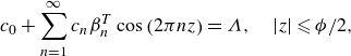 \begin{align}&\quad c_0 + \sum _{n=1}^\infty c_n \beta _n^T\cos \left (2\pi n z\right ) = \Lambda, \quad |z| \leqslant \phi / 2, \end{align}
where $\alpha _n^T=-1$
and
$\alpha _n^T=-1$
and $\beta _n^T=-2 \pi n \Lambda \coth (2 \pi n\Lambda )$
.
$\beta _n^T=-2 \pi n \Lambda \coth (2 \pi n\Lambda )$
.
Next, we multiply both (A3) and (A4) by $\cos (2 m \pi z)$
for
$\cos (2 m \pi z)$
for $m \in [0, N]$
, where
$m \in [0, N]$
, where $N$
is chosen to numerically truncate the summation. We then integrate the equations after multiplication over the interval
$N$
is chosen to numerically truncate the summation. We then integrate the equations after multiplication over the interval $\phi / 2 \lt z \leqslant 1 / 2$
and the interval
$\phi / 2 \lt z \leqslant 1 / 2$
and the interval $0\leqslant z \leqslant \phi / 2$
, respectively. Finally, we sum the results to obtain dual-series algebraic equations as
$0\leqslant z \leqslant \phi / 2$
, respectively. Finally, we sum the results to obtain dual-series algebraic equations as
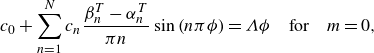 \begin{equation} c_0+\sum _{n=1}^{N} c_n \frac {\beta ^{T}_n-\alpha ^{T}_n}{\pi n} \sin \left (n \pi \phi \right )=\Lambda \phi \quad \text{for} \quad m=0, \end{equation}
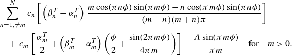 \begin{equation} \begin{aligned} &\sum _{n=1,\neq m}^{N} c_n \left [\left (\beta _n^T-\alpha _n^T\right )\frac {m\cos (\pi n\phi )\sin (\pi m\phi )-n\cos (\pi m\phi )\sin (\pi n\phi )}{(m-n)(m+n)\pi } \right ] \\ &\quad+\, c_m \left [\frac {\alpha ^{T}_m}{2}+\left (\beta ^{T}_m-\alpha ^{T}_m\right )\left (\frac {\phi }{2}+\frac {\sin (2 \pi m \phi )}{4 \pi m}\right )\right ] = \frac {\Lambda \sin (\pi m \phi )}{ \pi m} \quad \text{for} \quad m\gt 0. \end{aligned} \end{equation}
Then we can write the equations in matrix form as
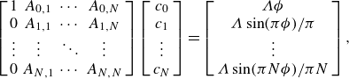 \begin{equation} \left [\begin{array}{cccc} 1 & A_{0,1} & \cdots & A_{0, N} \\ 0 & A_{1,1} & \cdots & A_{1, N} \\ \vdots & \vdots & \ddots & \vdots \\ 0 & A_{N,1} & \cdots & A_{N, N} \end{array}\right ]\left [\begin{array}{c} c_0 \\ c_1 \\ \vdots \\ c_{N} \end{array}\right ]=\left [\begin{array}{c} \Lambda \phi \\ \Lambda \sin (\pi \phi )/\pi \\ \vdots \\ \Lambda \sin (\pi N \phi )/\pi N \end{array}\right ], \end{equation}
where $A_{m,n}$
is defined for
$A_{m,n}$
is defined for $m=0$
,
$m=0$
, $m=n$
or
$m=n$
or $m \neq n$
:
$m \neq n$
:
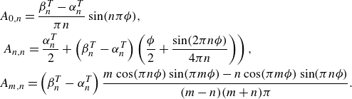 \begin{equation} \begin{aligned} & A_{0,n}=\frac {\beta _n^T-\alpha _n^T}{ \pi n} \sin (n \pi \phi ), \\ & \left .A_{n,n}=\frac {\alpha _n^T}{2}+\left (\beta _n^T-\alpha _n^T\right )\left (\frac {\phi }{2}+\frac {\sin (2 \pi n \phi )}{4 \pi n}\right )\right ), \\ & A_{m,n}=\left (\beta _n^T-\alpha _n^T\right )\frac {m \cos (\pi n \phi ) \sin (\pi m \phi )-n \cos (\pi m \phi ) \sin (\pi n \phi )}{(m-n)(m+n) \pi }. \end{aligned} \end{equation}
Appendix B. Thermal slip length
$\boldsymbol{\lambda}_{\boldsymbol{{t,c}}}$
on curved gas–liquid interface

Substituting the perturbation expansion for temperature $T=T^{(0)}+\epsilon T^{(1)}+O (\epsilon ^2 )$
into (2.22) we obtain a series of equations at different orders of
$T=T^{(0)}+\epsilon T^{(1)}+O (\epsilon ^2 )$
into (2.22) we obtain a series of equations at different orders of $\epsilon$
. At
$\epsilon$
. At $O(\epsilon ^0)$
, we have
$O(\epsilon ^0)$
, we have
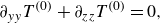 \begin{equation} \partial _{y y} T^{(0)} + \partial _{zz} T^{(0)}=0, \end{equation}
with the boundary conditions as
 \begin{equation} \begin{aligned} & T^{(0)}(\Lambda, z)=0\\ & \left \{\begin{array}{ll} T^{(0)}(0, z)=0, & \phi /2\lt |z| \leqslant 1 / 2 \\ \partial _y T^{(0)}(0, z)=0, & |z| \leqslant \phi /2, \end{array} \right . \end{aligned} \end{equation}
which is exactly the case of the flat interface and has been solved in § 2.2.1 and Appendix A, namely $T^{(0)}=T_p+T_s$
.
$T^{(0)}=T_p+T_s$
.
At $O(\epsilon ^1)$
, the problem is formulated as
$O(\epsilon ^1)$
, the problem is formulated as
 \begin{equation} \partial _{y y} T^{(1)}+\partial _{zz} T^{(1)}=0, \end{equation}
with the boundary conditions
 \begin{align}&\qquad\qquad\qquad\qquad\qquad\qquad T^{(1)}(\Lambda, z)=0, \end{align}
 \begin{align}& \left \{\begin{array}{ll} T^{(1)}(0, z)=0, & \phi /2\lt |z| \leqslant 1 / 2, \\ \partial _y T^{(1)}(0, z)=\eta \partial _{y y} T^{(0)}(0, z)-\eta ^{\prime } \partial _z T^{(0)}(0, z), & |z| \leqslant \phi /2 . \end{array} \right . \end{align}
The general solution of the first-order temperature ${T}^{(1)}=\tilde {T}^{(1)}/\Lambda$
, where
${T}^{(1)}=\tilde {T}^{(1)}/\Lambda$
, where $\tilde {T}^{(1)}$
has the same form as (2.12), i.e.
$\tilde {T}^{(1)}$
has the same form as (2.12), i.e.
 \begin{equation} \tilde {T}^{(1)} (y, z)= c_0^{(1)} \frac {y}{\Lambda } + d_0^{(1)} + \sum _{n=1}^\infty \left [c_n^{(1)} \cosh \left (2\pi n y\right ) + d_n^{(1)} \sinh \left (2\pi n y\right )\right ] \cos \left (2\pi n z\right ). \end{equation}
Applying boundary condition (B4) gives
 \begin{equation} {T}^{(1)}=c_0^{(1)}(y-\Lambda )+\sum _{n=1}^{\infty } c_n^{(1)} \frac {\sinh \left [2\pi n(\Lambda -y)\right ]}{\sinh \left (2\pi n \Lambda \right )} \cos \left (2\pi n z\right ). \end{equation}
Then, applying conditions (B5) in (B7) yields
 \begin{equation} \begin{gathered} c_0^{(1)}+\sum _{n=1}^{\infty } c_n^{(1)} \alpha ^{T}_n \cos \left (2\pi n z\right )=0, \quad \phi /2 \lt |z| \leqslant 1/2, \\ c_0^{(1)}+\sum _{n=1}^{\infty } c_n^{(1)} \beta ^{T}_n \cos \left (2\pi n z\right )= -\Lambda \partial _z\left (\eta \partial _z \tilde {T}^{(0)}(0, z)\right ), \quad |z| \leqslant \phi /2, \end{gathered} \end{equation}
where
 \begin{equation} -\Lambda \partial _z\left (\eta \partial _z \tilde {T}^{(0)}(0, z)\right ) = \sum _{n=1}^{\infty } \Lambda c_n \left [2\pi n \sin \left (2\pi n z\right )\eta ^{\prime }+(2\pi n)^2 \cos \left (2\pi n z\right )\eta \right ]. \end{equation}
Similarly, dual series equations can be obtained by multiplying these equations by $\cos (2\pi m z )$
, integrating over the corresponding domain and summing them. The dual series equations also can be solved numerically by the same procedure as in Appendix A. Nevertheless, we can immediately find
$\cos (2\pi m z )$
, integrating over the corresponding domain and summing them. The dual series equations also can be solved numerically by the same procedure as in Appendix A. Nevertheless, we can immediately find
 \begin{equation} c_0^{(1)}=0, \end{equation}
because every term equals 0 for $m=0$
. Now, we can notice that mean heat flux
$m=0$
. Now, we can notice that mean heat flux $\left \langle q^{\prime \prime }\right \rangle _c$
across
$\left \langle q^{\prime \prime }\right \rangle _c$
across $y=\Lambda$
is
$y=\Lambda$
is
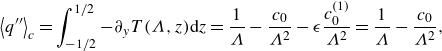 \begin{equation} \left \langle q^{\prime \prime }\right \rangle _c = \int _{-1/2}^{1/2}-\partial _yT(\Lambda, z){\textrm d}z= \frac {1}{\Lambda }-\frac {c_0}{\Lambda ^2}-\epsilon \frac {c_0^{(1)}}{\Lambda ^2}=\frac {1}{\Lambda }-\frac {c_0}{\Lambda ^2}, \end{equation}
which reveals that the presence of the meniscus has no influence on the average heat flux, i.e. $\lambda _{t,c}=\lambda _{t,f}$
.
$\lambda _{t,c}=\lambda _{t,f}$
.
Appendix C. Procedure for solving for the longitudinal slip length
$\boldsymbol{\lambda}_{\boldsymbol{\parallel,} \boldsymbol{{f}}}$

The general solution of $\tilde {u}$
along the parallel grooves is
$\tilde {u}$
along the parallel grooves is
 \begin{equation} \begin{aligned} \tilde {u} (y,z) = r_0 +q_{0}\frac {y}{\Lambda }+\sum _{n=1}^\infty \left [r_n\cosh \left (2\pi n y\right )+q_n \sinh \left (2\pi n y\right )\right ] \cos \left (2\pi n z\right ), \end{aligned} \end{equation}
where $r_n$
and
$r_n$
and $q_n$
are constants to be determined. Substitution of (2.26) results in
$q_n$
are constants to be determined. Substitution of (2.26) results in
 \begin{equation} q_0=-r_0, \quad q_n=-r_n \coth \left (2\pi n\Lambda \right ). \end{equation}
Then (2.27) results in
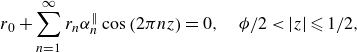 \begin{align}& r_0+\sum _{n=1}^{\infty } r_n\alpha ^{\|}_n \cos \left (2\pi n z\right )=0, \quad \phi /2 \lt |z| \leqslant 1/2, \end{align}
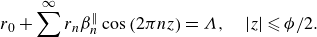 \begin{align}&\quad r_0+\sum ^{\infty } r_n\beta ^{\parallel }_n \cos \left (2\pi n z\right )=\Lambda, \quad |z| \leqslant \phi /2. \end{align}
The coefficients of $\alpha ^{\parallel }_n$
and
$\alpha ^{\parallel }_n$
and $\beta ^{\parallel }_n$
are
$\beta ^{\parallel }_n$
are
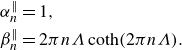 \begin{equation} \begin{aligned} \alpha ^{\|}_n & =1, \\ \beta ^{\|}_n & =2\pi n\Lambda \coth (2\pi n\Lambda ). \end{aligned} \end{equation}
Following what are now standard steps, we also can obtain the dual-series algebraic equations as
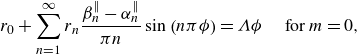 \begin{align}&\qquad\qquad\qquad r_0+\sum _{n=1}^{\infty } r_n \frac {\beta ^{\parallel }_n-\alpha ^{\parallel }_n}{\pi n} \sin \left (n \pi \phi \right )=\Lambda \phi \quad \text{ for } m=0, \end{align}
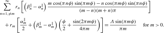 \begin{align}& \sum _{n=1,\neq m}^{\infty } r_n \left [\left (\beta _n^{\parallel }-\alpha _n^{\parallel }\right ) \frac {m\cos (\pi n\phi )\sin (\pi m\phi )-n\cos (\pi m\phi )\sin (\pi n\phi )}{(m-n)(m+n)\pi }\right ] \nonumber\\ &\quad + r_m \left [\frac {\alpha ^{\parallel }_m}{2}+\left (\beta ^{\parallel }_m-\alpha ^{\parallel }_m\right )\left (\frac {\phi }{2}+\frac {\sin (2 \pi m \phi )}{4 \pi m}\right )\right ] = \frac {\Lambda \sin (\pi m \phi )}{ \pi m}\quad \text{ for } m\gt 0. \end{align}
Equations (C5a
)–(C5b
) can be numerically solved for $r_0$
and
$r_0$
and $r_n$
for
$r_n$
for $m \in [0, N]$
and
$m \in [0, N]$
and $n \in [0, N]$
.
$n \in [0, N]$
.
Appendix D. Procedure for solving
$\boldsymbol{\lambda} _{\boldsymbol{\parallel} \boldsymbol{{.c}}}$

Substituting the perturbation velocity $u=u^{(0)}+\epsilon u^{(1)}+O (\epsilon ^2 )$
into (2.36) we obtain a series of equations at different orders of
$u=u^{(0)}+\epsilon u^{(1)}+O (\epsilon ^2 )$
into (2.36) we obtain a series of equations at different orders of $\epsilon$
. At
$\epsilon$
. At $O(\epsilon ^0)$
, we have
$O(\epsilon ^0)$
, we have
 \begin{equation} \partial _{zz} u^{(0)}+\partial _{y y} u^{(0)}=-\partial _xP, \end{equation}
 \begin{equation} \begin{aligned} & u^{(0)}(\Lambda, z)=0\\ & \left \{\begin{array}{ll} u^{(0)}(0, z)=0, & \phi /2\lt |z| \leqslant 1 / 2 \\ \partial _y u^{(0)}(0, z)=0, & |z| \leqslant \phi /2 \end{array} \right ., \end{aligned} \end{equation}
which is the case of the flat meniscus and has been treated in Appendix C. Hence $r_n^{(0)}=r_n$
and
$r_n^{(0)}=r_n$
and
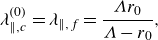 \begin{equation} \lambda _{\parallel, c}^{(0)} = \lambda _{\parallel, f}=\frac {\Lambda r_0}{\Lambda - r_0}, \end{equation}
where $r_0$
is the coefficient determined by numerically solving (C5a
)–(C5b
).
$r_0$
is the coefficient determined by numerically solving (C5a
)–(C5b
).
At $O(\epsilon ^1)$
, the equations are
$O(\epsilon ^1)$
, the equations are
 \begin{equation} \partial _{zz} u^{(1)}+\partial _{y y} u^{(1)}=0, \end{equation}
 \begin{equation} u^{(1)}(\Lambda, z)=0, \end{equation}
 \begin{equation} \left \{\begin{array}{ll} u^{(1)}(0, z)=0, & \phi /2\lt |z| \leqslant 1 / 2, \\ \partial _y u^{(1)}(0, z)=\eta \partial _{y y} u^{(0)}(0, z)-\eta ^{\prime } \partial _z u^{(0)}(0, z), & |z| \leqslant \phi /2 . \end{array} \right . \end{equation}
The general solution of the first-order velocity ${u}^{(1)}=-\partial _xP\Lambda \tilde {u}^{(1)}/2$
, where
${u}^{(1)}=-\partial _xP\Lambda \tilde {u}^{(1)}/2$
, where $\tilde {u}^{(1)}$
has the same form as (C1), i.e.
$\tilde {u}^{(1)}$
has the same form as (C1), i.e.
 \begin{equation} \tilde {u}^{(1)}=r_0^{(1)} +q_0^{(1)}\frac {y}{\Lambda }+\sum _{n=1}^{\infty }\left [r_n^{(1)} \cosh \left (2\pi n y\right )+q_n^{(1)} \sinh \left (2\pi n y\right )\right ] \cos \left (2\pi n z\right ). \end{equation}
Applying the boundary condition (D5) leads to
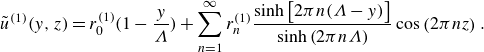 \begin{equation} \tilde {u}^{(1)}(y,z)=r_0^{(1)}(1-\frac {y}{\Lambda })+\sum _{n=1}^{\infty } r_n^{(1)} \frac {\sinh \left [2\pi n(\Lambda -y)\right ]}{\sinh \left (2\pi n \Lambda \right )} \cos \left (2\pi n z\right ). \end{equation}
Then applying condition (D6) in (D8) yields
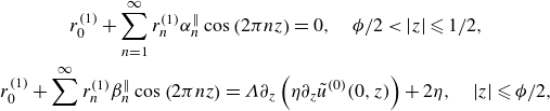 \begin{equation} \begin{gathered} r_0^{(1)}+\sum _{n=1}^{\infty } r_n^{(1)} \alpha ^{\|}_n \cos \left (2\pi n z\right )=0, \quad \phi /2 \lt |z| \leqslant 1/2, \\ r_0^{(1)}+\sum ^{\infty } r_n^{(1)} \beta ^{\parallel }_n \cos \left (2\pi n z\right )= \Lambda \partial _z\left (\eta \partial _z \tilde {u}^{(0)}(0, z)\right )+2\eta, \quad |z| \leqslant \phi /2, \end{gathered} \end{equation}
where
 \begin{equation} \partial _z\left (\eta \partial _z \tilde {u}^{(0)}(0, z)\right ) = \sum _{n=1}^{\infty } r_n \left [-2\pi n \sin \left (2\pi n z\right )\eta ^{\prime }-(2\pi n)^2 \cos \left (2\pi n z\right )\eta \right ] . \end{equation}
Similarly, dual series equations can be obtained by multiplying by $\cos (2\pi m z )$
and integrating. The dual series equations also can be solved numerically using the same procedure as in Appendix A,
$\cos (2\pi m z )$
and integrating. The dual series equations also can be solved numerically using the same procedure as in Appendix A,
 \begin{align}&\qquad\qquad r_0^{(1)}+\sum _{n=1}^{\infty } r_n^{(1)} \frac {\beta ^{\parallel }_n-\alpha ^{\parallel }_n}{\pi n} \sin \left (n \pi \phi \right )=\frac {4\phi ^3}{3} \quad \text{for} \quad m=0, \end{align}
 \begin{align}& \sum _{n=1,\neq m}^{\infty } r_n^{(1)} \left [\left (\beta _n^{\parallel }-\alpha _n^{\parallel }\right ) \frac {1}{2 \pi }\left (\frac {\sin (\pi (m+n) \phi )}{m+n}+\frac {\sin (\pi (m-n) \phi )}{m-n}\right )\right ] \notag\\ &\quad + r_m^{(1)} \left [\frac {\alpha ^{\parallel }_m}{2}+\left (\beta ^{\parallel }_m-\alpha ^{\parallel }_m\right )\left (\frac {\phi }{2}+\frac {\sin (2 \pi m \phi )}{4 \pi m}\right )\right ] = \mathcal{M}\left (n,m,\Lambda, \phi \right ) \quad \text{for} \quad m\gt 0, \end{align}
where the function $\mathcal{M} (n,m,\Lambda, \phi )$
is
$\mathcal{M} (n,m,\Lambda, \phi )$
is
 \begin{equation} \begin{aligned} \mathcal{M}\left (n,m,\Lambda, \phi \right ) &= \, \frac {4\sin (\pi \phi m) - 4\pi \phi m \cos (\pi \phi m)}{ \pi ^3 m^3} +\sum _{n=1,\neq m}^{\infty }\frac {4r_n \Lambda m n}{(m-n)^3(m+n)^3 \pi }\\ &\left \{m\cos (m \pi \phi )\left [2 n\left (m^2-n^2\right ) \pi \phi \cos (n \pi \phi )+\left (m^2+3 n^2\right ) \sin (n \pi \phi )\right ]\right . \\ & \left . +\sin (m \pi \phi )\left [-n\left (3 m^2+n^2\right ) \cos (n \pi \phi )+\left (m^4-n^4\right ) \pi \phi \sin (n \pi \phi )\right ]\right \}\\ &+ r_m\Lambda \left ( \frac {3 \sin (2 m \pi \phi )-8 m^3 \pi ^3 \phi ^3-6 m \pi \phi \cos (2 m \pi \phi )}{12 m \pi } \right ) . \end{aligned} \end{equation}
Appendix E. Representative temperature and velocity fields above longitudinal grooves
Taking the gas–liquid ratio $\phi = 0.3$
as an example, we examine the variation in aspect ratio
$\phi = 0.3$
as an example, we examine the variation in aspect ratio $\Lambda = 0.1, 0.5$
and
$\Lambda = 0.1, 0.5$
and $2.5$
. The corresponding temperature and velocity field visualizations are shown in figure 8. Here, the normalised quantity
$2.5$
. The corresponding temperature and velocity field visualizations are shown in figure 8. Here, the normalised quantity $ u^{(0)}/(-\partial _x P)$
represents the velocity field assuming a flat gas–liquid interface, whereas the total velocity
$ u^{(0)}/(-\partial _x P)$
represents the velocity field assuming a flat gas–liquid interface, whereas the total velocity $u/(-\partial _x P)$
accounts for the influence of the curved meniscus. From figure 8, it is evident that decreasing
$u/(-\partial _x P)$
accounts for the influence of the curved meniscus. From figure 8, it is evident that decreasing $\Lambda$
significantly amplifies the effect of slip. In contrast, for
$\Lambda$
significantly amplifies the effect of slip. In contrast, for $\Lambda = 2.5$
, the influence of slip in both the temperature and velocity fields appears negligible. Moreover, when the curved meniscus is considered, the velocity distribution remains largely unchanged in terms of spatial variation, but its absolute magnitude is noticeably enhanced. However, it is challenging to directly infer the variation of the corresponding effective slip length with
$\Lambda = 2.5$
, the influence of slip in both the temperature and velocity fields appears negligible. Moreover, when the curved meniscus is considered, the velocity distribution remains largely unchanged in terms of spatial variation, but its absolute magnitude is noticeably enhanced. However, it is challenging to directly infer the variation of the corresponding effective slip length with $\Lambda$
from the changes in the temperature and velocity fields.
$\Lambda$
from the changes in the temperature and velocity fields.
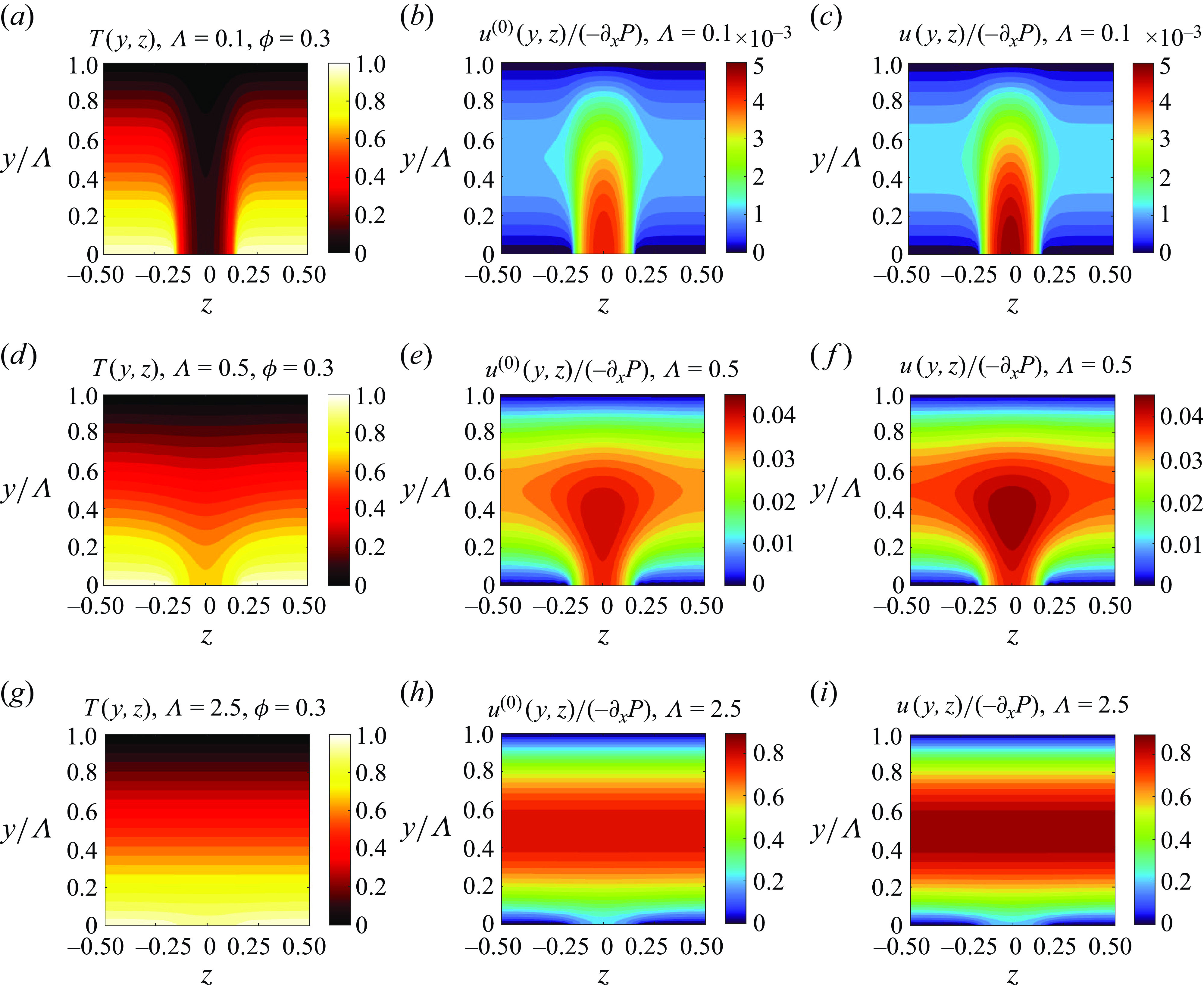
Figure 8. Representative (a,d,g) temperature field $T(y,z)$
, (b,e,f) normalised leading-order velocity
$T(y,z)$
, (b,e,f) normalised leading-order velocity $u^{(0)}(y,z)/(-\partial _xP)$
distribution considering the flat gas–liquid interface and (c,f,g) total normalised velocity
$u^{(0)}(y,z)/(-\partial _xP)$
distribution considering the flat gas–liquid interface and (c,f,g) total normalised velocity $u(y,z)/(-\partial _xP)$
considering the curved interface. Panels (a–c), (d–e) and (g–f) correspond to
$u(y,z)/(-\partial _xP)$
considering the curved interface. Panels (a–c), (d–e) and (g–f) correspond to $\Lambda =0.1$
, 0.5 and 2.5, respectively, while
$\Lambda =0.1$
, 0.5 and 2.5, respectively, while $\phi =0.3$
is fixed.
$\phi =0.3$
is fixed.
Appendix F. Slip length
$\boldsymbol{\lambda} _{\boldsymbol{\perp,} \boldsymbol{{f}}}$
on transverse grooves with a flat liquid–gas interface

The general solution of the deviation component of the stream function $\tilde {\Psi }$
between two parallel plates with transverse grooves, is well known as (Lauga & Stone Reference Lauga and Stone2003; Teo & Khoo Reference Teo and Khoo2008)
$\tilde {\Psi }$
between two parallel plates with transverse grooves, is well known as (Lauga & Stone Reference Lauga and Stone2003; Teo & Khoo Reference Teo and Khoo2008)
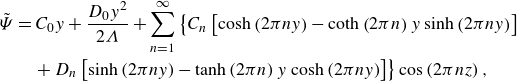 \begin{align} \tilde {\Psi } & = C_0 y+\frac {D_0 y^2}{2\Lambda }+\sum _{n=1}^{\infty }\left \{C_n\left [\cosh \left (2\pi n y\right )-\operatorname {coth}\left (2\pi n\right ) y \sinh \left (2\pi n y\right )\right ]\right . \nonumber \\ & \quad \left .+\, D_n\left [\sinh \left (2\pi n y\right )-\tanh \left (2\pi n\right ) y \cosh \left (2\pi n y\right )\right ]\right \} \cos \left (2\pi n z\right ), \end{align}
where $x$
and
$x$
and $y$
are, respectively, the coordinates along width and height in the cross-section of flow, and
$y$
are, respectively, the coordinates along width and height in the cross-section of flow, and $C_0$
,
$C_0$
, $D_0$
,
$D_0$
, $C_n$
and
$C_n$
and $D_n$
are unknown coefficients determined by specific boundary conditions;
$D_n$
are unknown coefficients determined by specific boundary conditions; $2\pi n$
represents the wavenumber. The boundary conditions for grooves on a single channel wall are
$2\pi n$
represents the wavenumber. The boundary conditions for grooves on a single channel wall are
 \begin{align}&\qquad\qquad\qquad \partial _y \tilde {\Psi }|_{y=\Lambda }=0, \end{align}
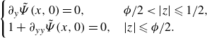 \begin{align}& \begin{cases} \partial _y \tilde {\Psi }(x,0)=0, & \phi /2 \lt |z| \leqslant 1/2, \\ 1+\partial _{yy} \tilde {\Psi }(x,0)=0, & |z|\leqslant \phi /2. \end{cases} \end{align}
Equation (F2) leads to
 \begin{equation} C_0 = -D_0,\quad C_n=D_n \gamma, \end{equation}
where
 \begin{align} \gamma =-\frac { 2\pi n \cosh \left (2\pi n\Lambda \right )- \tanh \left (2\pi n\right )\cosh \left (2\pi n\Lambda \right )- 2\pi n\Lambda \tanh \left (2\pi n\right ) \sinh \left (2\pi n\Lambda \right )} {2\pi n \sinh \left (2\pi n\Lambda \right )-\coth \left (2\pi n\right )\sinh \left (2\pi n\Lambda \right )-2\pi n\Lambda \operatorname {coth}\left (2\pi n\right ) \cosh \left (2\pi n\Lambda \right ) } . \end{align}
Also, (F3) leads to
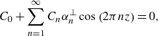 \begin{equation} C_0+\sum _{n=1}^{\infty } C_n \alpha ^{\perp }_{n} \cos \left (2\pi n z\right )=0, \end{equation}
for $\phi /2 \lt |z| \leqslant 1/2$
and
$\phi /2 \lt |z| \leqslant 1/2$
and
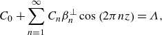 \begin{equation} C_0+\sum _{n=1}^{\infty } C_n \beta ^{\perp }_{n} \cos \left (2\pi n z\right )=\Lambda, \end{equation}
for $|z| \leqslant \phi /2$
. The coefficient
$|z| \leqslant \phi /2$
. The coefficient $\alpha ^{\perp }_{n}$
and
$\alpha ^{\perp }_{n}$
and $\beta ^{\perp }_{n}$
are
$\beta ^{\perp }_{n}$
are
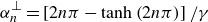 \begin{equation} \begin{aligned} \alpha ^{\perp }_{n}= \left [ 2 n \pi -\tanh \left (2 n \pi \right )\right ]/\gamma \end{aligned} \end{equation}
and
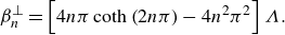 \begin{equation} \begin{aligned} \beta ^{\perp }_{n}= \left [4n\pi \coth \left (2n\pi \right )-4n^2\pi ^2\right ]\Lambda . \end{aligned} \end{equation}
Finally,
 \begin{equation} \lambda _{\perp } = \frac {\Lambda C_0}{\Lambda -C_0}. \end{equation}
Similar to the approach in the last section, values of $C_0$
and
$C_0$
and $C_n$
can be numerically solved by replacing
$C_n$
can be numerically solved by replacing $\alpha ^{\|}$
and
$\alpha ^{\|}$
and $\beta ^{\|}$
with
$\beta ^{\|}$
with $\alpha ^{\perp }$
and
$\alpha ^{\perp }$
and $\beta ^{\perp }$
, respectively.
$\beta ^{\perp }$
, respectively.
Appendix G. Numerical approach for solving for the solid height
$\boldsymbol{{H}}\boldsymbol{(\tau )}$
and film thickness
$\boldsymbol{{h}}\boldsymbol{(\tau )}$
of gravity-driven CCM


Recalling (2.52a
) and (2.52b
) with $\mathscr{c}=1$
, we can rewrite them by defining the functions
$\mathscr{c}=1$
, we can rewrite them by defining the functions $f(\Lambda )$
and
$f(\Lambda )$
and $g(\Lambda )$
, respectively, as
$g(\Lambda )$
, respectively, as
 \begin{equation} \Lambda ^4\frac {1+4\lambda /\Lambda }{1+\lambda /\Lambda }\left (1+\frac {\lambda _{t}}{\Lambda }\right ) \equiv f(\Lambda )=\frac {1}{Hl^4},\end{equation}
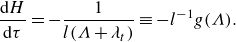 \begin{equation} \frac {{\textrm d}H}{{\textrm d}\tau }=-\frac {1}{l(\Lambda +\lambda _{t})} \equiv -l^{-1} g(\Lambda ) . \end{equation}
Using (G1a
) and (G1b
) and the initial condition $H(\tau =0)=1$
, we can numerically compute
$H(\tau =0)=1$
, we can numerically compute $H$
through the following discrete iterative equations:
$H$
through the following discrete iterative equations:
 \begin{align}&\qquad f(\Lambda ^i)=l^{-4}\frac {1}{H^i}, \end{align}
 \begin{align}& H^{i+1}= -l^{-1} g(\Lambda ^{i}) \tau _\delta +H^{i}, \end{align}
where the superscript $i$
represents the time step, and
$i$
represents the time step, and $\tau _\delta$
denotes the time increment. This implies that
$\tau _\delta$
denotes the time increment. This implies that $\Lambda ^{i}$
can be determined using
$\Lambda ^{i}$
can be determined using $H^{i}$
at the current time step
$H^{i}$
at the current time step $i$
via (G2a
). Subsequently,
$i$
via (G2a
). Subsequently, $H^{i+1}$
can be calculated by substituting
$H^{i+1}$
can be calculated by substituting $\Lambda ^{i}$
into (G2b
). However, since the functions
$\Lambda ^{i}$
into (G2b
). However, since the functions $f(\Lambda )$
and
$f(\Lambda )$
and $g(\Lambda )$
do not have analytical expressions, it is necessary to precompute a sufficient number of discrete values for these functions for a specific
$g(\Lambda )$
do not have analytical expressions, it is necessary to precompute a sufficient number of discrete values for these functions for a specific $\phi$
. During the iteration process, interpolation is used to obtain
$\phi$
. During the iteration process, interpolation is used to obtain $f(\Lambda )$
and
$f(\Lambda )$
and $g(\Lambda )$
for any given
$g(\Lambda )$
for any given $\Lambda$
based on discrete results. The functions
$\Lambda$
based on discrete results. The functions $f_{\parallel, c}(\Lambda )$
and
$f_{\parallel, c}(\Lambda )$
and $g(\Lambda )$
for longitudinal grooves, considering the meniscus interface, are plotted in figures 9(a) and 9(b), respectively. Since the
$g(\Lambda )$
for longitudinal grooves, considering the meniscus interface, are plotted in figures 9(a) and 9(b), respectively. Since the $f_{\parallel, f}(\Lambda )$
for flat interfaces is very similar to that for meniscus interfaces, figure 9(c) presents the ratio of
$f_{\parallel, f}(\Lambda )$
for flat interfaces is very similar to that for meniscus interfaces, figure 9(c) presents the ratio of $f_{\parallel, f}(\Lambda )$
for flat interfaces to
$f_{\parallel, f}(\Lambda )$
for flat interfaces to $f_{\parallel, c}(\Lambda )$
for meniscus interfaces.
$f_{\parallel, c}(\Lambda )$
for meniscus interfaces.
Figure 9. Functions of (a) $f_{\parallel, c}(\Lambda )$
and (b)
$f_{\parallel, c}(\Lambda )$
and (b) $g(\Lambda )$
for the meniscus interface on longitudinal grooves for iterative numerical approaches, and (c) the ratio
$g(\Lambda )$
for the meniscus interface on longitudinal grooves for iterative numerical approaches, and (c) the ratio $f_{\parallel, f}(\Lambda )/f_{\parallel, c}(\Lambda )$
of flat to curved interface. Dotted line represents no-slip.
$f_{\parallel, f}(\Lambda )/f_{\parallel, c}(\Lambda )$
of flat to curved interface. Dotted line represents no-slip.
Appendix H. Asymptotic solutions of
$\boldsymbol{{H}}\boldsymbol{(\tau )}$
and corresponding conditions for the gravity-driven mode

With the given asymptotic formulae of slip lengths in table 1, we can derive the asymptotic solutions and their conditions for $H-\tau$
. Considering the range of
$H-\tau$
. Considering the range of $\Lambda \gtrsim 0.2$
, substitution of (3.12) into (3.18a
) yields
$\Lambda \gtrsim 0.2$
, substitution of (3.12) into (3.18a
) yields
 \begin{equation} h = k_{1}H^{-\frac {1}{4}}, \quad \Lambda \gtrsim 0.2, \end{equation}
where $k_{1}$
is given as
$k_{1}$
is given as
 \begin{align} &k_{1} = \nonumber\\&\left (\!\frac {1 + \frac {1}{\Lambda \pi } \ln \left (\sec \left (\frac {\phi \pi }{2}\right )\right ) + \frac {\epsilon }{\Lambda } \left (-\phi ^3 \mathcal{F}(\phi ) + \frac {4}{\Lambda } \phi ^4 \mathcal{G}(\phi )\right ) \left (1 + \frac {1}{4\Lambda \pi } \ln \left (\sec \left (\frac {\phi \pi }{2}\right )\right )\right )^2}{1 + \frac {4}{\Lambda \pi } \ln \left (\sec \left (\frac {\phi \pi }{2}\right )\right ) + \frac {4\epsilon }{\Lambda } \left (-\phi ^3 \mathcal{F}(\phi ) + \frac {4}{\Lambda } \phi ^4 \mathcal{G}(\phi )\right ) \left (1 + \frac {1}{4\Lambda \pi } \ln \left (\sec \left (\frac {\phi \pi }{2}\right )\right )\right )^2} \!\right )^\frac {1}{4} \nonumber\\ &\left (1 + \frac {4}{\Lambda \pi } \ln \left (\sec \left (\frac {\phi \pi }{2}\right )\right )\right )^{-\frac {1}{4}}, \end{align}
and is plotted in figure 10(a). It demonstrated that only for $\Lambda = 1-10$
and small
$\Lambda = 1-10$
and small $\phi$
,
$\phi$
, $k_{1}$
can be considered as approximately equal to 1, which is consistent with the results in figures 6(c) and 6(d). Especially, when
$k_{1}$
can be considered as approximately equal to 1, which is consistent with the results in figures 6(c) and 6(d). Especially, when $\Lambda \gtrsim 10$
, we can further simplify (H2) as follows:
$\Lambda \gtrsim 10$
, we can further simplify (H2) as follows:
 \begin{equation} h = \left ({1+\frac {4}{\Lambda \pi }\ln (\sec \frac {\phi \pi }{2})}\right )^{-\frac {1}{4}}H^{-\frac {1}{4}} \equiv k_{2}H^{-\frac {1}{4}},\quad \Lambda \gtrsim 10. \end{equation}
By numerically analysing the order of $k_{\Lambda \geqslant 10}$
, it is found to have a magnitude of
$k_{\Lambda \geqslant 10}$
, it is found to have a magnitude of $\sim 1$
within the range
$\sim 1$
within the range $\Lambda = 10 - 10^{3}$
, as depicted in figure 10(b), although with a smaller deviation for large
$\Lambda = 10 - 10^{3}$
, as depicted in figure 10(b), although with a smaller deviation for large $\phi$
. Therefore, it is reasonable to approximate the above equation as
$\phi$
. Therefore, it is reasonable to approximate the above equation as
 \begin{equation} h \approx H^{-\frac {1}{4}}, \end{equation}
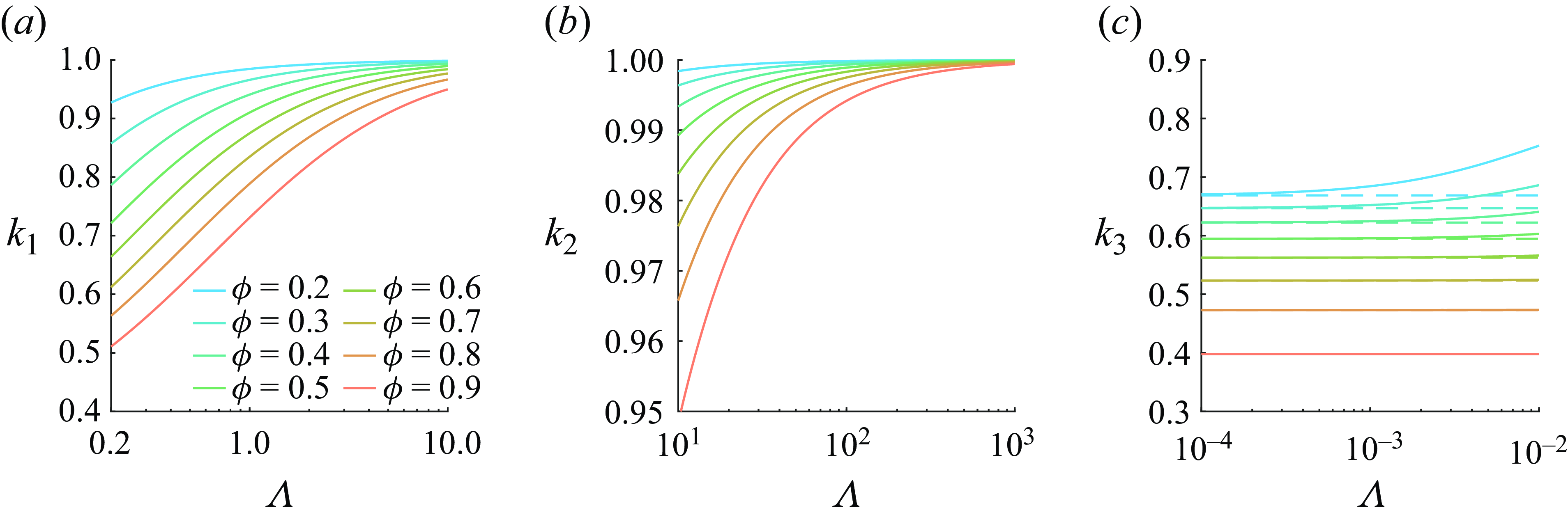
Figure 10. Variations of coefficients (a) $k_1$
, (b)
$k_1$
, (b) $k_2$
and (c)
$k_2$
and (c) $k_3$
versus aspect ratio
$k_3$
versus aspect ratio $\Lambda$
.
$\Lambda$
.
which is exactly equivalent to (3.19a
) and (3.19b
) for the no-slip condition. To satisfy the condition $\Lambda \gtrsim 10$
, it follows that
$\Lambda \gtrsim 10$
, it follows that
 \begin{equation} l \lesssim 0.1, \end{equation}
due to the necessary condition $h(\tau =0)/l \gtrsim 10$
.
$h(\tau =0)/l \gtrsim 10$
.
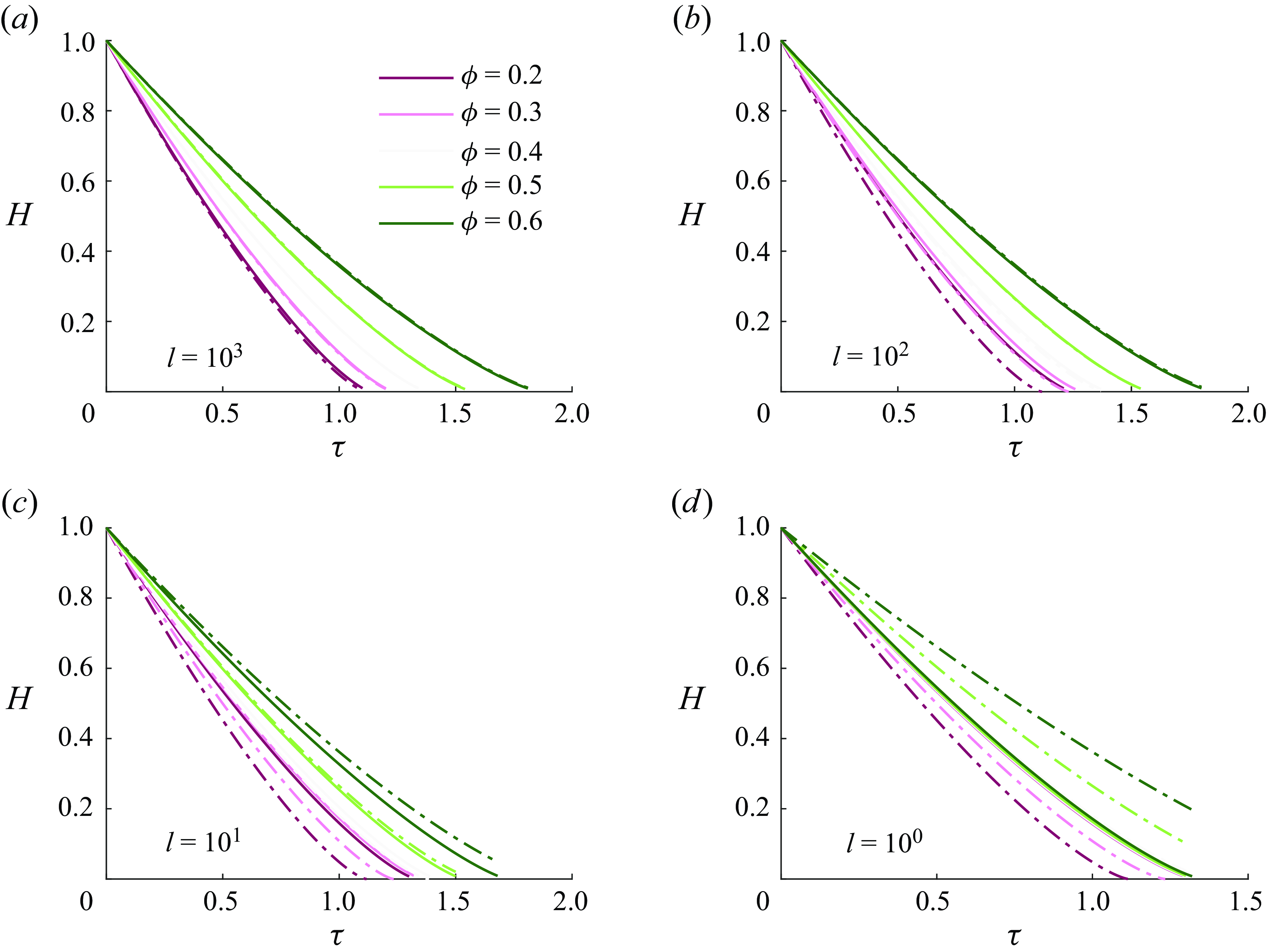
Figure 11. Non-dimensional height $ H(\tau )$
of solid PCM, comparing numerical results with asymptotic solutions (3.21), i.e. (H11), at
$ H(\tau )$
of solid PCM, comparing numerical results with asymptotic solutions (3.21), i.e. (H11), at $ l =$
(a)
$ l =$
(a) $ 10^3$
, (b)
$ 10^3$
, (b) $ 10^2$
, (c)
$ 10^2$
, (c) $ 10^1$
and (d)
$ 10^1$
and (d) $ 10^0$
for
$ 10^0$
for $\phi$
values ranging from 0.2 to 0.6. Solid lines represent numerical results, while dot–dash lines indicate asymptotic solutions.
$\phi$
values ranging from 0.2 to 0.6. Solid lines represent numerical results, while dot–dash lines indicate asymptotic solutions.
As for the range of $\Lambda \lesssim 0.01$
, we can substitute (3.11) into (G1a
), yielding
$\Lambda \lesssim 0.01$
, we can substitute (3.11) into (G1a
), yielding
 \begin{equation} h = \Bigg [1+\frac {1}{\dfrac {1}{3}+\dfrac {4}{3}\dfrac {\phi }{1-\phi }+\dfrac {8\sin \theta }{9\Lambda }\dfrac {\phi ^2}{(1-\phi )^2}}\Bigg ]^{\frac {1}{4}} \left (\frac {1-\phi }{4}\right )^{\frac {1}{4}}H^{-\frac {1}{4}} \equiv k_{3}H^{-\frac {1}{4}}, \quad \Lambda \lesssim 0.01. \end{equation}
By plotting $k_{3}$
along with
$k_{3}$
along with $\Lambda$
in figure 10(c), it demonstrates that
$\Lambda$
in figure 10(c), it demonstrates that $k_{3}$
remains constant for
$k_{3}$
remains constant for $\phi = 0.5 - 0.9$
while deviates greater for smaller
$\phi = 0.5 - 0.9$
while deviates greater for smaller $\phi \leqslant 0.4$
. We can easily obtain the asymptotic profile for
$\phi \leqslant 0.4$
. We can easily obtain the asymptotic profile for $\phi = 0.5\!-\!0.9$
is
$\phi = 0.5\!-\!0.9$
is $(1-\phi )^{0.25}/4^{0.25}$
as plotted as a dashed line in figure 7(d). Therefore, the maximum film thickness at the end
$(1-\phi )^{0.25}/4^{0.25}$
as plotted as a dashed line in figure 7(d). Therefore, the maximum film thickness at the end $h_{end}$
is
$h_{end}$
is
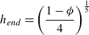 \begin{equation} h_{end} = \left ( \frac {1-\phi }{4}\right )^{\frac {1}{5}} \end{equation}
by letting $H = h_{end}$
. Then one limit condition for
$H = h_{end}$
. Then one limit condition for $h_{end}/l \lesssim 0.01$
is
$h_{end}/l \lesssim 0.01$
is
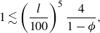 \begin{equation} 1 \lesssim \left ( \frac {l}{100}\right )^5 \frac {4}{1-\phi }, \end{equation}
which is plotted as black dot–dash lines in figure 7(a). Another limit condition lies in
 \begin{equation} \frac {1}{3}+\frac {4}{3}\frac {\phi }{1-\phi }+\frac {8\sin \theta }{9\Lambda }\frac {\phi ^2}{(1-\phi )^2} \gg 1, \end{equation}
which can be derived to give
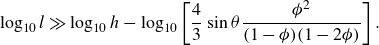 \begin{equation} \log _{10}{l} \gg \log _{10}{h} -\log _{10}\left [{\frac {4}{3}\sin \theta \frac {\phi ^2}{(1-\phi )(1-2\phi )}}\right ]. \end{equation}
By adopting $h=h_{max}=10$
from the no-slip condition, this condition is plotted as white dot–dashed lines in figure 7(a). Therefore, the upper right-hand region enclosed by the two dash–dotted lines represents the parameter range where the following asymptotic solution is valid:
$h=h_{max}=10$
from the no-slip condition, this condition is plotted as white dot–dashed lines in figure 7(a). Therefore, the upper right-hand region enclosed by the two dash–dotted lines represents the parameter range where the following asymptotic solution is valid:
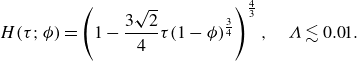 \begin{equation} H(\tau ;\phi )= \left (1-\frac {3\sqrt {2}}{4}\tau (1-\phi )^{\frac {3}{4}} \right )^{\frac {4}{3}}, \quad \Lambda \lesssim 0.01. \end{equation}


 Open access