


1. Introduction
The aortic regurgitation, or insufficiency, is the reverse flow of blood from the aorta into the left ventricle (LV) in large amounts during the cardiac diastole due to an inadequate closure of the native aortic valve, primarily resulting from the malcoaptation of the valve’s leaflets (Bekeredjian & Grayburn Reference Bekeredjian and Grayburn2005; Perez & Dager Reference Perez and Dager2023). Since the aortic regurgitation/insufficiency is directly related to the closure kinematics of aortic valves, an investigation of the latter has historically been a topic of peculiar research interest. In 1513, Leonardo da Vinci realised the presence of the dilatation of the aorta at three locations (later termed as the sinuses) behind each cusp of the native aortic valve. He predicted the formation of vortices in the aortic sinuses and that they might influence the closure kinematics of the aortic valve (Bellhouse & Talbot Reference Bellhouse and Talbot1969; Ming & Zhen-huang Reference Ming and Zhen-huang1986). However, according to Bellhouse & Talbot (Reference Bellhouse and Talbot1969), da Vinci might have mistakenly attributed blood circulation and other flow features as vortices in the sinuses.
Modern investigations on the closure dynamics of natural heart valves started with the ‘vortex theory’ of Bellhouse & Talbot (Reference Bellhouse and Talbot1969), who experimentally investigated the dynamics of a trapped vortex in the sinuses under steady and pulsatile aortic flow conditions. The opening mechanism of the aortic valve was not modelled, primarily due to the assumption of inviscid flow, which might only be valid for the valve closure phase (Lee & Talbot Reference Lee and Talbot1979). They observed that a sinus vortex is generated primarily by the convective effects due to a combined ‘inflow–outflow’ process through each sinus. By analytically modelling the sinus vortex as one-half of a Hill spherical vortex, Bellhouse & Talbot (Reference Bellhouse and Talbot1969) reported that it complements the axial adverse pressure gradient in pushing the cusps to their fully closed position during the flow deceleration. Van Steenhoven & Van Dongen (Reference Van Steenhoven and Van Dongen1979) conducted experiments in a two-dimensional (2-D) analogue to investigate the closure of aortic valves. They reported that the adverse pressure gradient developed during the flow deceleration phase of the cardiac cycle is itself sufficient to close the cusps, without requiring assistance from any trapped vortex in the sinus. The flow deceleration in their experiments started from a steady state, which might not adequately represent the aortic flow conditions. Lee & Talbot (Reference Lee and Talbot1979) reported that a pressure difference across the valves’ cusps is only developed due to the flow deceleration, and the sinus vortex may not complement it in closing the cusps. Later studies by Wippermann (Reference Wippermann1985) and Ming & Zhen-huang (Reference Ming and Zhen-huang1986) also suggested that the major closure phase during the flow deceleration is solely caused by the axial adverse pressure gradient, which disturbs the balance on the two surfaces of the cusps (central flow- and the sinus-side). In the studies discussed so far, the experiments were complemented by simplified one-dimensional (1-D)/2-D analytical models for native aortic valves (without consideration to their elastic deformations) and a spatial three-dimensional (3-D) distribution of the pressure on the two sides of the leaflets/cusps of the aortic valves was not presented to support the claim that a difference of pressure forces causes the valves’ closure.
The native aortic valve malfunctioning with aortic regurgitation in specific, or any other valvular disease in general, might require a replacement through surgical intervention. In accordance with the American College of Cardiology/American Heart Association (ACC/AHA) valvular heart diseases guidelines (Coisne et al. Reference Coisne2023), the surgical aortic valve replacement is typically recommended in patients with symptomatic severe aortic regurgitation, and in asymptomatic patients demonstrating severe aortic regurgitation alongside the LV’s dysfunction with a progressive decline in the ejection fraction and/or enlargement (Malahfji et al. Reference Malahfji, Saeed and Zoghbi2023). The available prosthetic replacements for a diseased aortic valve may be classified into two types: mechanical heart valves (MHVs) and bioprosthetic heart valves (BHVs). The current designs of MHVs could be further classified as trileaflet MHVs (TMHVs) and bileaflet MHVs (BMHVs). The TMHVs have three leaflets which close by rotating towards the centre, i.e. the tip of the leaflet moves towards the centre (figure 1), similar to the native aortic valves/BHVs, whereas the BMHV leaflets move towards the sinuses for closure (figure 1). It is well known that the healthy natural valves/BHVs fully close by the end of systole (i.e. zero flow), thereby inhibiting any regurgitation volume (Yoganathan et al. Reference Yoganathan, He and Casey Jones2004; Mohammadi & Mequanint Reference Mohammadi and Mequanint2011; Borazjani Reference Borazjani2013; Sotiropoulos et al. Reference Sotiropoulos, Le and Gilmanov2016), whereas the BMHV leaflets begin their closure at the onset of the regurgitation during early diastole. The BMHVs therefore allow a regurgitant volume of around 2–7 ml per beat (Bottio et al. Reference Bottio, Caprili, Casarotto and Gerosa2004; Dumont et al. Reference Dumont, Vierendeels, Kaminsky, van Nooten, Verdonck and Bluestein2007; Li et al. Reference Li, Chen, Lo and Lu2011) which is relatively higher than that in the native valves/BHVs (Yoganathan et al. Reference Yoganathan, Chandran and Sotiropoulos2005; Borazjani & Sotiropoulos Reference Borazjani and Sotiropoulos2010; Abbas et al. Reference Abbas, Nasif, Al-Waked and Said2020a ).

Figure 1. Closure directions (orange arrows) and jets of typical TMHV, natural aortic valves/BHV and BMHV.
The hemodynamics of the TMHVs, BMHVs and BHVs have been investigated previously, but the reasons behind the delayed closure of the BMHV and whether it could be improved has yet to be clarified. Lu et al. (Reference Lu, Liu, Huang, Lo, Lai and Hwang2004) employed digital particle image velocimetry to compare the closure behaviour of several designs of MHVs, being a TMHV, a BMHV and a monoleaflet MHV. They reported that the MHVs generate vortices in the aortic sinuses during the cardiac flow acceleration, which promote the closure of a TMHV during the flow deceleration while impeding the closure of the BMHV and the monoleaflet MHV. Their experimental results were not supported by analytical modelling to fully resolve the vorticity dynamics of the MHVs, and a 3-D imaging of the movement of the leaflets could not be obtained. In addition, the augmentation of the adverse pressure gradient by the sinus vortices to efficiently close the TMHV was not explained. Li et al. (Reference Li, Chen, Lo and Lu2011) used digital particle image velocimetry to compare the leaflet kinematics and hemodynamics of a TMHV with a BMHV. The presence of vortices in the aortic sinus was claimed to cause the closure initiation of the TMHV, whereas the reverse flow initiated the closure kinematics of the BMHV. However, the details of the local pressure field and the fluid moments acting on the two valves, and their interaction with the vortices, were not reported to explain the closing behaviours. Vennemann et al. (Reference Vennemann, Rösgen, Heinisch and Obrist2018) experimentally observed a similar closing behaviour between a BHV and a TMHV, being smooth and early during the cardiac cycle compared with a BMHV. While the authors mentioned that the difference of the flow fields may generate different pressure fields to enable an early closure of the TMHV and BHV in comparison with the BMHV, they did not explicitly measure/report the variations in the pressure on the valves’ leaflets. The BMHV closed abruptly; however, the reason behind this behaviour was not explored.
In a numerical study, Li & Lu (Reference Li and Lu2012) maintained that the leaflets of the TMHV started to fully close during the systolic deceleration and demonstrated a slower closing velocity compared with the leaflets of the BMHV, that were pushed to closure by regurgitation. While the study identified the vortices in the aortic sinuses as the reason for the early TMHV closure compared with the BMHV based on the vortex theory of Bellhouse & Talbot (Reference Bellhouse and Talbot1969), the interaction between the vorticity dynamics and the adverse pressure gradient for the TMHV was neither mathematically modelled nor discussed. Borazjani et al. (Reference Borazjani, Ge and Sotiropoulos2010a ) hypothesised that the difference of the pressure field on the two sides of the leaflets in artificial heart valves might explain the differences in their closure dynamics (without consideration to the sinus vortices); however, they neither made distinct comparisons between different valves nor reported a distribution of pressure across their leaflets. In fact, as noted in Chen & Luo (Reference Chen and Luo2020), generally the published numerical and experimental analysis of artificial heart valves has lacked the investigation of the spatial pressure distribution on the valves’ leaflets.
Recapitulating, a review of the studies discussed above reveals that the fluid dynamical reasons behind the early closure of the TMHVs and BHVs, and a delayed closure of the BMHVs are still not fully understood. Whether an adverse pressure gradient during the cardiac deceleration is sufficient to induce the closure of an aortic artificial heart valve, without requiring assistance from the sinus vortices, is still an open question. We strive to obtain a conclusive view by conducting 3-D fluid–structure interaction (FSI) simulations of a TMHV, a BMHV and a BHV under similar conditions to identify the underlying mechanism behind the closure of these valves and address this question. Following the discussion of the local pressure field and related hemodynamics, our simulations suggest design principles specifically aimed at achieving early closure and reducing the regurgitant volume of artificial heart valves (see § 5).
This paper is organised ahead as follows: § 2 provides the details of the valves’ models and the numerical methodology; § 3 presents the results for the leaflet kinematics and hemodynamics of the three valves; § 4 discusses the results and lists the limitations of the study; whereas § 5 provides a recapitulation of all the reported findings and concludes with general design guidelines for early closure of the valve.
2. Materials and methodology
2.1. Geometric modelling
For the TMHV in this study, the design of the TRIFLO Valve (Novostia, Switzerland) has been selected. It is composed of three leaflets, made up of polyether ether ketone with a density of 1300 kg m− $^3$
, housed at a symmetry of
$^3$
, housed at a symmetry of $120^\circ$
without the conventional recessed hinges in a housing containing inflow and outflow stops. The leaflets could therefore be considered hingeless or ‘floating’ with no fixed point. The TMHV, as visualised from the aorta in its fully closed and fully opened states, has been illustrated by figures 2(ai) and 2(aii), respectively. Figure 2(aiii) details one of the three leaflets of the TMHV, which are all slightly curved and wedge-shaped, with a height (h) of 15.865 mm, length (l) of 11.88 mm and a leading-edge thickness of 0.516 mm, varying over the length of each leaflet. The BHV model employed in the current simulations also has three leaflets, modelled as nonlinear, membrane-like, thin shell structures composed of anisotropic material undergoing deformations to replicate the experimentally observed stress–strain behaviour of a heart valve tissue (Borazjani Reference Borazjani2013; Asadi & Borazjani Reference Asadi and Borazjani2023). Figures 2(bi) and 2(bii), respectively, illustrate the fully closed and fully opened states of the BHV, whereas figure 2(biii) shows one of its three leaflets in its elastically deformed, opened position. The leaflets of the BHV have a uniform thickness of 0.386 mm, with elastically varying lengths and heights in a three-fold symmetry, housed in a cylinder. For the BMHV, the design of the On-X Valve (Artivion, formerly CryoLife Inc., USA) is selected for this study. The hinge recess in the housing and the hinges for the BMHV leaflets were not modelled as these regions require extraordinarily fine meshing to obtain fully resolved flow features, which could be computationally cumbersome. The two leaflets of the BMHV are made up of pyrolytic carbon, with a density of 2200 kg m−
$120^\circ$
without the conventional recessed hinges in a housing containing inflow and outflow stops. The leaflets could therefore be considered hingeless or ‘floating’ with no fixed point. The TMHV, as visualised from the aorta in its fully closed and fully opened states, has been illustrated by figures 2(ai) and 2(aii), respectively. Figure 2(aiii) details one of the three leaflets of the TMHV, which are all slightly curved and wedge-shaped, with a height (h) of 15.865 mm, length (l) of 11.88 mm and a leading-edge thickness of 0.516 mm, varying over the length of each leaflet. The BHV model employed in the current simulations also has three leaflets, modelled as nonlinear, membrane-like, thin shell structures composed of anisotropic material undergoing deformations to replicate the experimentally observed stress–strain behaviour of a heart valve tissue (Borazjani Reference Borazjani2013; Asadi & Borazjani Reference Asadi and Borazjani2023). Figures 2(bi) and 2(bii), respectively, illustrate the fully closed and fully opened states of the BHV, whereas figure 2(biii) shows one of its three leaflets in its elastically deformed, opened position. The leaflets of the BHV have a uniform thickness of 0.386 mm, with elastically varying lengths and heights in a three-fold symmetry, housed in a cylinder. For the BMHV, the design of the On-X Valve (Artivion, formerly CryoLife Inc., USA) is selected for this study. The hinge recess in the housing and the hinges for the BMHV leaflets were not modelled as these regions require extraordinarily fine meshing to obtain fully resolved flow features, which could be computationally cumbersome. The two leaflets of the BMHV are made up of pyrolytic carbon, with a density of 2200 kg m− $^3$
, and have a height (h) of 16.3 mm, length (l) of 11.62 mm and a uniform thickness of 0.710 mm. Figures 2(ci) and 2(cii), illustrate the fully closed and fully opened states of the BMHV, whereas figure 2(ciii) shows one of its two leaflets.
$^3$
, and have a height (h) of 16.3 mm, length (l) of 11.62 mm and a uniform thickness of 0.710 mm. Figures 2(ci) and 2(cii), illustrate the fully closed and fully opened states of the BMHV, whereas figure 2(ciii) shows one of its two leaflets.
The three valves have an external diameter of 21 mm and an internal diameter of 19.6 mm, and the two MHVs can undergo a maximum rotation of $50^\circ$
in response to the cardiac flow (
$50^\circ$
in response to the cardiac flow ( $\theta _{minimum}=0^\circ$
and
$\theta _{minimum}=0^\circ$
and $\theta _{maximum}=50^\circ$
). There are no stops for the excursion of the BHVs. The aortic root is configured as a rigid and straight aorta without any curvature, however, with varying cross-sectional diameters along its length, as illustrated in figure 2(d). It is characterised by three bulged, axisymmetric sinuses, and has an inlet diameter of D = 25.82 mm. The three valves are located at the initial tract of the aorta, at a streamwise/axial distance of
$\theta _{maximum}=50^\circ$
). There are no stops for the excursion of the BHVs. The aortic root is configured as a rigid and straight aorta without any curvature, however, with varying cross-sectional diameters along its length, as illustrated in figure 2(d). It is characterised by three bulged, axisymmetric sinuses, and has an inlet diameter of D = 25.82 mm. The three valves are located at the initial tract of the aorta, at a streamwise/axial distance of $\approx$
2.8D from the inlet.
$\approx$
2.8D from the inlet.

Figure 2. The geometric models of (a) the TMHV, (b) the BHV, (c) the BMHV and (d) the aortic root.
2.2. Numerical method
The incompressible Navier–Stokes equations alongside the continuity equation constitute the set of governing partial differential equations for the blood flow inside human aorta. To solve these equations under a stretched grid configuration, the curvilinear immersed boundary (CurvIB) method as presented by Ge & Sotiropoulos (Reference Ge and Sotiropoulos2007), has been used as a flow solver in this study. When employing CurvIB, the governing equations are first transformed from the cartesian coordinates to the curvilinear coordinates and are written as
 \begin{align}&\qquad\qquad\qquad\qquad J\displaystyle \frac {\partial V^r}{\partial \zeta ^r}=0 ,\end{align}
 \begin{align} \displaystyle \frac {\partial V^r}{\partial t}&=-\displaystyle \frac {\zeta _{q}^r}{J}\left [J\frac {\partial (V^pu_q)}{\partial \zeta ^p}-\frac {1}{Re}J\frac {\partial \left(\frac {g^{pm}}{J}\frac {\partial u_q}{\partial \zeta ^m} \right)}{\partial \zeta ^p}\right ]-\zeta _{q}^r\displaystyle \frac {\partial \left(\zeta _{q}^p\frac {P}{J} \right)}{\partial \zeta ^p},\end{align}
where, $V^r$
is the surface volume flux, such that
$V^r$
is the surface volume flux, such that $V^r=U^r/J$
,
$V^r=U^r/J$
, $U^r$
is the contravariant velocity components,
$U^r$
is the contravariant velocity components, $J$
is the Jacobian of the geometric transformation such that
$J$
is the Jacobian of the geometric transformation such that $J=\displaystyle {\partial (\zeta ^1,\zeta ^2,\zeta ^3)}/{\partial (x^1,y^2,z^3)}$
,
$J=\displaystyle {\partial (\zeta ^1,\zeta ^2,\zeta ^3)}/{\partial (x^1,y^2,z^3)}$
, $P$
is the non-dimensional pressure,
$P$
is the non-dimensional pressure, $u_q$
is the cartesian velocity while
$u_q$
is the cartesian velocity while $g^{pm}$
is the contravariant metric tensor, such that
$g^{pm}$
is the contravariant metric tensor, such that $g^{pm}=\zeta _{xq}^p\zeta _{xq}^m$
.
$g^{pm}=\zeta _{xq}^p\zeta _{xq}^m$
.
The convective terms in (2.2) are discretised in space by employing quadratic upstream interpolation for convective kinematics scheme, whereas the viscous terms are discretised by using the central difference scheme. The equations are advanced in time by using a fractional step method (Ge & Sotiropoulos Reference Ge and Sotiropoulos2007; Borazjani et al. Reference Borazjani, Ge and Sotiropoulos2008). The momentum equations are solved implicitly (Asgharzadeh & Borazjani Reference Asgharzadeh and Borazjani2017), followed by the pressure-Poisson equation which is solved by the generalised minimal residual method with multigrid preconditioning. The velocity and pressure are corrected by the obtained pressure correction from the pressure-Poisson equation. No turbulence model is used in this work because previous simulations with our code (Borazjani et al. Reference Borazjani, Ge and Sotiropoulos2008) have been shown to accurately capture the transitional flow features when compared with parallel experiments (Dasi et al. Reference Dasi, Ge, Simon, Sotiropoulos and Yoganathan2007).
The incompressible flow equations are to be solved in a domain enclosed by the aortic lumen and having the dynamic leaflets’ boundaries immersed inside it. Such simulations therefore require intricate FSI modelling to establish the interaction between blood (fluid) and valves’ leaflets (structure). In this study, the CurvIB method is strongly coupled with a robust FSI algorithm to calculate the leaflet kinematics of the TMHV, the BHV and the BMHV. For the TMHV and the BMHV, the FSI algorithm constitutes of the equations for rigid body motion with a single degree of freedom, being rotation only, as detailed by Borazjani et al. (Reference Borazjani, Ge and Sotiropoulos2008). For the BHV simulations, a novel contact model is employed in a rotation-free, large deformation, thin shell finite element framework (Asadi & Borazjani Reference Asadi and Borazjani2023), which is based on Loop’s subdivision surfaces (Cirak et al. Reference Cirak, Ortiz and Schröder2000; Cirak & Ortiz Reference Cirak and Ortiz2001). The robust contact modelling algorithm continuously interpolates the displacement field on the triangular grid and has been validated against several benchmark problems (Asadi & Borazjani Reference Asadi and Borazjani2023). The nonlinear and anisotropic material model developed by Kim et al. (Reference Kim, Lu, Sacks and Chandran2008) for a typical bovine pericardial BHV with asymmetric fiber direction of $45^{\circ}$
forms the leaflets’ constitutive equations for their bending and membrane response. For all valves, generally, four to six (04–06) subiterations were required for the strongly coupled FSI model to achieve convergence within each time step during the opening and closing phases of the valves, whereas a single subiteration sufficed for fully opened valves.
$45^{\circ}$
forms the leaflets’ constitutive equations for their bending and membrane response. For all valves, generally, four to six (04–06) subiterations were required for the strongly coupled FSI model to achieve convergence within each time step during the opening and closing phases of the valves, whereas a single subiteration sufficed for fully opened valves.
The in-house CurvIB code is parallelised with MPI and PETSc to efficiently utilise the supercomputing facilities at our disposal. The CurvIB solver has been extensively validated in the past (Borazjani et al. Reference Borazjani, Ge and Sotiropoulos2008; Borazjani & Sotiropoulos Reference Borazjani and Sotiropoulos2009; Borazjani et al. Reference Borazjani, Ge, Le and Sotiropoulos2013; Asgharzadeh & Borazjani Reference Asgharzadeh and Borazjani2017; Hedayat et al. Reference Hedayat, Akbarzadeh and Borazjani2022; Asadi & Borazjani Reference Asadi and Borazjani2023) and successfully applied to various cardiovascular flows (Borazjani et al. Reference Borazjani, Ge and Sotiropoulos2010a ; Hedayat et al. Reference Hedayat, Asgharzadeh and Borazjani2017; Asgharzadeh & Borazjani Reference Asgharzadeh and Borazjani2019; Asgharzadeh et al. Reference Asgharzadeh, Asadi, Meng and Borazjani2019; Hedayat & Borazjani Reference Hedayat and Borazjani2019; Asadi et al. Reference Asadi, Hedayat and Borazjani2022), and other applications (Borazjani et al. Reference Borazjani, Sotiropoulos, Malkiel and Katz2010b ; Simmons et al. Reference Simmons, Daghooghi and Borazjani2023).
2.3. Computational set-up
The simulations start from a zero-flow initial condition with the valves’ leaflets in their fully closed position and have been carried out for multiple cardiac cycles. The results from the second cycle are used per our analysis of the cycle-to-cycle variations, which is reported in Appendix A. A no-slip boundary condition was imposed on the surfaces of the housing and the leaflets of the three valves. A cardiac flow pulse with a plug (uniform) profile has been prescribed at the inlet of the computational domain, as shown in figure 3(a), whereas a convective boundary condition (Neumann condition with a correction for mass balance) is applied at the outflow (Borazjani et al. Reference Borazjani, Ge and Sotiropoulos2008; Borazjani et al. Reference Borazjani, Ge and Sotiropoulos2010a
; Asadi et al. Reference Asadi, Hedayat and Borazjani2022). The inlet and outlet locations are far enough from the valve such that the location of the boundary does not influence the solution (Borazjani et al. Reference Borazjani, Ge and Sotiropoulos2008). The flow pulse (figure 3
a) was provided by the parallel experiments conducted at ARTORG Center for Biomedical Engineering Research, University of Bern, Switzerland, with a maximum inflow rate of $Q_{max}=3.424\times 10^{-4}$ $\rm m^3$
s−1. While different prosthetic valves have different retrograde flow profiles, to facilitate the comparison between valves under similar conditions, the same flow curve was employed for the three valves in this study similar to previous comparative studies (Li & Lu Reference Li and Lu2012; Nitti et al. Reference Nitti, De Cillis and de Tullio2022). A maximum retrograde flow of
$\rm m^3$
s−1. While different prosthetic valves have different retrograde flow profiles, to facilitate the comparison between valves under similar conditions, the same flow curve was employed for the three valves in this study similar to previous comparative studies (Li & Lu Reference Li and Lu2012; Nitti et al. Reference Nitti, De Cillis and de Tullio2022). A maximum retrograde flow of $Q=-0.24\times Q_{max}$
, followed by a constant 2 % adverse flow was prescribed to simulate the diastolic conditions, which are in a similar range as previous studies (Lee et al. Reference Lee, Rygg, Kolahdouz, Rossi, Retta, Duraiswamy, Scotten, Craven and Griffith2020; Asadi et al. Reference Asadi, Hedayat and Borazjani2022; Nitti et al. Reference Nitti, De Cillis and de Tullio2022). The sensitivity of the conclusions regarding the start of closure to the maximum retrograde flow is investigated in Appendix E.
$Q=-0.24\times Q_{max}$
, followed by a constant 2 % adverse flow was prescribed to simulate the diastolic conditions, which are in a similar range as previous studies (Lee et al. Reference Lee, Rygg, Kolahdouz, Rossi, Retta, Duraiswamy, Scotten, Craven and Griffith2020; Asadi et al. Reference Asadi, Hedayat and Borazjani2022; Nitti et al. Reference Nitti, De Cillis and de Tullio2022). The sensitivity of the conclusions regarding the start of closure to the maximum retrograde flow is investigated in Appendix E.
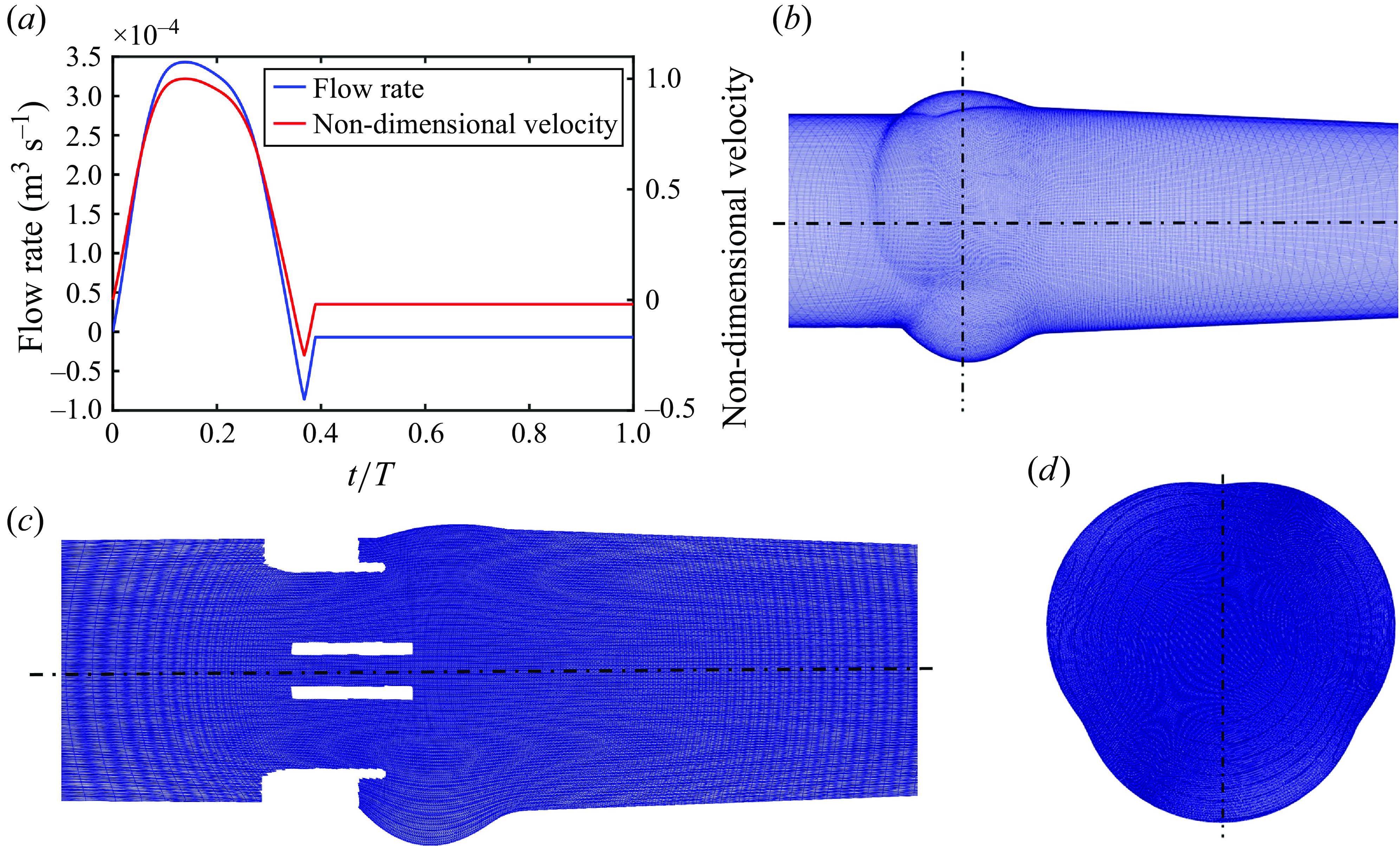
Figure 3. (a) The prescribed flow rate and the non-dimensional inlet velocity, (b) the curvilinear grid for the fluid domain, (c) the stretch of the grid shown for the BMHV domain (same for all valves) and (d) a cross-section of the grid in the sinuses.
The governing equations have been non-dimensionalised by the inlet aortic diameter of D = $25.82\times 10^{-3}$
m and the peak systolic velocity of U = 0.6548 m s−1, corresponding to a peak systolic Reynolds number of Re = 3620. The blood was modelled as a Newtonian fluid, having a density of 1200 kg
$25.82\times 10^{-3}$
m and the peak systolic velocity of U = 0.6548 m s−1, corresponding to a peak systolic Reynolds number of Re = 3620. The blood was modelled as a Newtonian fluid, having a density of 1200 kg $\rm m^{-3}$
and a viscosity of
$\rm m^{-3}$
and a viscosity of $5.6\times 10^{-3}$
N s
$5.6\times 10^{-3}$
N s $\rm m^{-2}$
. The cardiac cycle comprises of time T = 0.85714 s with a heart rate of 70 beats per minute. The temporal discretisation of the cardiac cycle was performed with 4350 time steps, which resulted from a time step independence study as discussed in Appendix B. The flow curve in figure 3(a) has been non-dimensionalised with U.
$\rm m^{-2}$
. The cardiac cycle comprises of time T = 0.85714 s with a heart rate of 70 beats per minute. The temporal discretisation of the cardiac cycle was performed with 4350 time steps, which resulted from a time step independence study as discussed in Appendix B. The flow curve in figure 3(a) has been non-dimensionalised with U.
Figure 3(b) illustrates the curvilinear grid on a section of the computational domain. The spatial discretisation of the computational domain was performed with $201\times 201\times 241 \approx 10\times 10^6$
grid points, by employing a stretched grid configuration (figure 3
c). A cross-section of the grid that encapsulates the aortic sinuses is also shown in figure 3(d). The grid is uniform in the vicinity of the valves and their immediate wake (in the region
$201\times 201\times 241 \approx 10\times 10^6$
grid points, by employing a stretched grid configuration (figure 3
c). A cross-section of the grid that encapsulates the aortic sinuses is also shown in figure 3(d). The grid is uniform in the vicinity of the valves and their immediate wake (in the region $2.75D \lt z/D \lt 3.75D$
from the inlet) with a non-dimensional grid size of 0.005, which is approximately twice of the Kolmogorov scale (
$2.75D \lt z/D \lt 3.75D$
from the inlet) with a non-dimensional grid size of 0.005, which is approximately twice of the Kolmogorov scale ( $\eta / D=Re^{-3/4}=0.0021$
), and then stretches to the inlet and outlet boundaries by using a hyperbolic tangent function. Previous direct numerical simulations of MHV flows, where the focus was on obtaining the turbulent statistics, were performed with a spatial resolution of 0.0035 (Yun et al. Reference Yun, Dasi, Aidun and Yoganathan2014a
) and 0.00356 (Nitti et al. Reference Nitti, De Cillis and de Tullio2022), which were considered reasonable to resolve the lower-order moments of turbulent MHV flows (Nitti et al. Reference Nitti, De Cillis and de Tullio2022). Our resolution is finer than the finest grid size investigated for mesh refinement in a study investigating the flow through aortic BHVs (Chen & Luo Reference Chen and Luo2020). Since (i) the focus of this work is not on the turbulent statistics, and (ii) the grid resolution adopted in the current study is similar to Borazjani et al. (Reference Borazjani, Ge and Sotiropoulos2008), which was found to be fine enough to capture all the flow features observed in the parallel experiments of Dasi et al. (Reference Dasi, Ge, Simon, Sotiropoulos and Yoganathan2007), the adopted resolution is deemed high enough for the current simulations.
$\eta / D=Re^{-3/4}=0.0021$
), and then stretches to the inlet and outlet boundaries by using a hyperbolic tangent function. Previous direct numerical simulations of MHV flows, where the focus was on obtaining the turbulent statistics, were performed with a spatial resolution of 0.0035 (Yun et al. Reference Yun, Dasi, Aidun and Yoganathan2014a
) and 0.00356 (Nitti et al. Reference Nitti, De Cillis and de Tullio2022), which were considered reasonable to resolve the lower-order moments of turbulent MHV flows (Nitti et al. Reference Nitti, De Cillis and de Tullio2022). Our resolution is finer than the finest grid size investigated for mesh refinement in a study investigating the flow through aortic BHVs (Chen & Luo Reference Chen and Luo2020). Since (i) the focus of this work is not on the turbulent statistics, and (ii) the grid resolution adopted in the current study is similar to Borazjani et al. (Reference Borazjani, Ge and Sotiropoulos2008), which was found to be fine enough to capture all the flow features observed in the parallel experiments of Dasi et al. (Reference Dasi, Ge, Simon, Sotiropoulos and Yoganathan2007), the adopted resolution is deemed high enough for the current simulations.
We assert that while both velocity (Dumont et al. Reference Dumont, Vierendeels, Kaminsky, van Nooten, Verdonck and Bluestein2007; Borazjani & Sotiropoulos Reference Borazjani and Sotiropoulos2010; Abbas et al. Reference Abbas, Nasif, Al-Waked and Said2020b ; Nitti et al. Reference Nitti, De Cillis and de Tullio2022) and pressure (Nicosia et al. Reference Nicosia, Cochran, Einstein, Rutland and Kunzelman2003; Marom et al. Reference Marom, Kim, Rosenfeld, Raanani and Haj-Ali2013) inlet boundary conditions have been used in the previous numerical studies of artificial heart valves, the employment of a staggered grid configuration for incompressible flows, as utilised by the CurvIB solver, only requires Dirichlet velocity boundary conditions for the problem to be well-posed (Gresho & Sani Reference Gresho and Sani1987). While a Dirichlet boundary condition for pressure and a Neumann boundary condition for velocity could also be applied, such a set-up drastically reduces the convergence rate of the pressure-correction methods for solving the governing incompressible Navier–Stokes equations (Guermond et al. Reference Guermond, Minev and Shen2006), as employed in the current study. It is not possible to apply both velocity and pressure conditions on the same boundary for incompressible flows or for flows with low compressibility (Marom Reference Marom2015). The adopted method for solving the pressure-Poisson equation and conservative nature of CurvIB with velocity boundary condition ensures that the pressure field is obtained such that the conservation of mass is satisfied to machine zero at each grid cell (Ge & Sotiropoulos Reference Ge and Sotiropoulos2007; Borazjani et al. Reference Borazjani, Ge and Sotiropoulos2008). This feature is important for pulsatile flow problems (like aortic conditions) in which the inflow changes should propagate instantly throughout the domain to enforce incompressibility.
3. Results
In this section, the numerical results from the computational FSI simulations of the TMHV, the BHV and the BMHV have been presented, compared and discussed. All the results are independent of the grid, time step size and the cardiac cycle-to-cycle variations. As previously mentioned, the grid independence and validation against parallel experiments of the BMHV (Dasi et al. Reference Dasi, Ge, Simon, Sotiropoulos and Yoganathan2007) was established in a previous work (Borazjani et al. Reference Borazjani, Ge and Sotiropoulos2008). Refer to Appendix A and Appendix B for further details of the analysis of the cardiac cycle-to-cycle variations and the time step independence study, respectively.
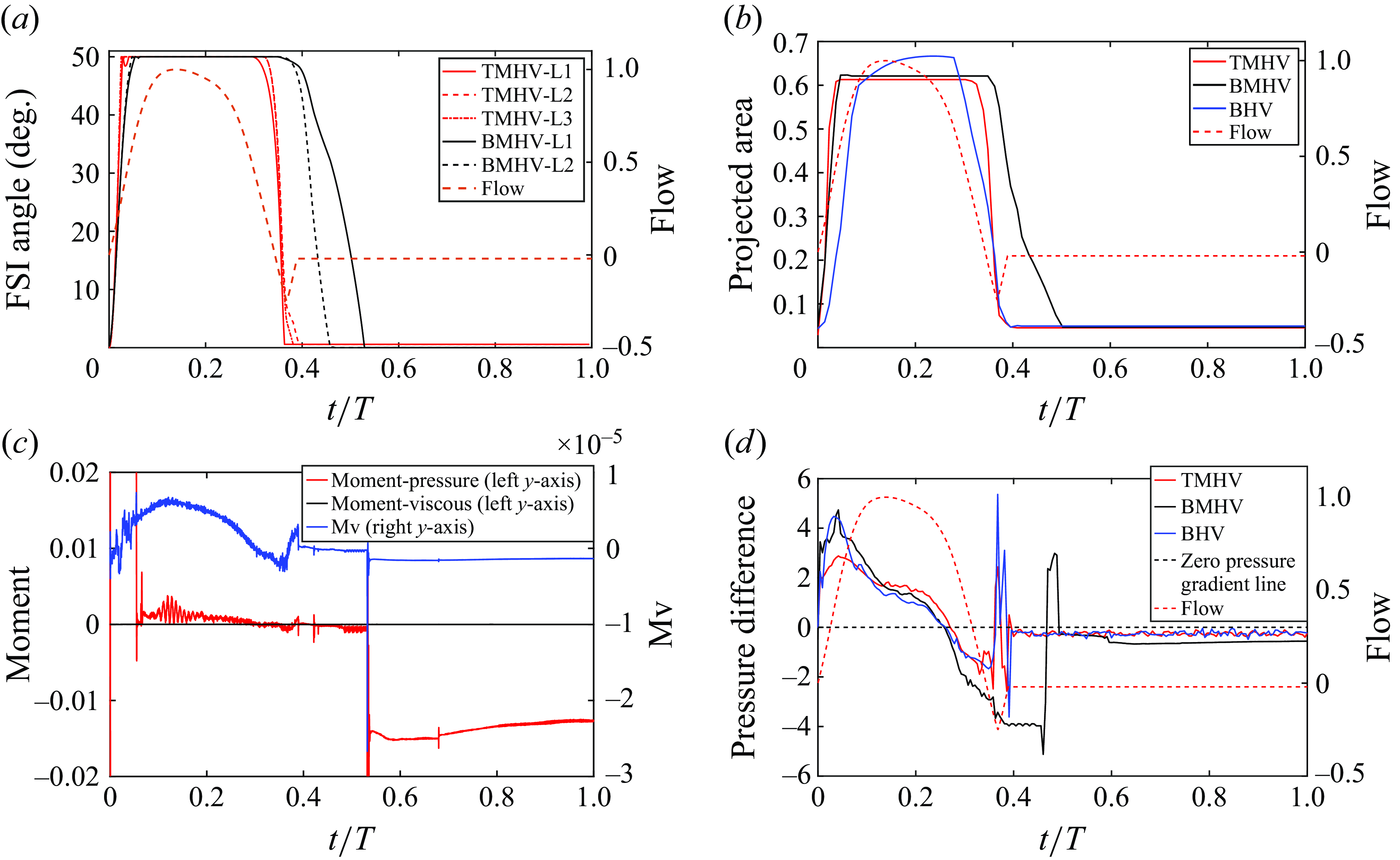
Figure 4. (a) Leaflet kinematics of the TMHV and BMHV (L1 corresponds to Leaflet 1, L2 to Leaflet 2 and L3 to Leaflet 3), (b) the non-dimensional projected area for the three valves (see Supplementary movie 1), (c) a comparison of pressure versus viscous moments and (d) the non-dimensional pressure difference.
3.1. Comparison of the leaflet kinematics of the three valves
The leaflet kinematics of the TMHV and the BMHV have been graphically compared in figure 4(a). Owing to the elastic excursions of the BHV leaflets, it is not possible to plot their FSI angles against time in a graphical form. However, the reader is referred to Appendix C for a discourse on the transient deformation and displacement of the BHV leaflets. For the TMHV, the three leaflets open in a slightly asynchronous pattern in response to the cardiac flow and reach their fully opened position after initially rebounding very little, with Leaflet 1 undergoing the maximum rebound in comparison with the other two leaflets. The leaflets of the BMHV take a relatively longer time to reach their fully opened position in comparison with the TMHV, with the BMHV getting fully opened around 16 ms after the full opening of the TMHV. While fully opened, the leaflets of the TMHV and BMHV do not exhibit any noticeable fluttering motion during the systolic phase. The TMHV starts to close during the systolic deceleration phase of the cardiac cycle and the three leaflets complete most of their closure excursion by the early regurgitation phase. Contrary to that, the BMHV starts undergoing its closure phase at the onset of regurgitation and fully closes late into the diastolic phase of the cardiac cycle. It could also be observed that the three leaflets close slightly asynchronously for the TMHV, with Leaflet 1 closing the earliest whereas Leaflet 2 closing the latest. The degree of the asynchronous motion of the two leaflets in the BMHV is, however, clearly higher compared with the TMHV leaflets during the valve closure.
To facilitate the comparison of the leaflet kinematics of the two MHVs with the BHV, the projected area on the plane perpendicular to the streamwise direction (the z-plane) for each valve, has been calculated by employing (3.1) and plotted against time in figure 4(b),
 \begin{equation} PA_v=\frac {\textit{IOA}_v-\sum _{i=1}^nPAL_i}{\textit{IOA}_{\textit{BHV}}} ,\end{equation}
where, $PA_v$
is the projected area of the valve on the z-plane,
$PA_v$
is the projected area of the valve on the z-plane, $IOA_v$
is the inner orifice area of the valve,
$IOA_v$
is the inner orifice area of the valve, $PAL_i$
is the projected area of the ‘ith’ leaflet, n is the number of leaflets in the valve, being three for the TMHV and the BHV, whereas two for the BMHV, while
$PAL_i$
is the projected area of the ‘ith’ leaflet, n is the number of leaflets in the valve, being three for the TMHV and the BHV, whereas two for the BMHV, while $IOA_{BHV}$
is the inner orifice area of the BHV, being the largest among all valves and therefore used for normalisation of the projected area.
$IOA_{BHV}$
is the inner orifice area of the BHV, being the largest among all valves and therefore used for normalisation of the projected area.
Figure 4(b) shows that the BHV has the largest projected area during the systolic phase of the cardiac cycle in comparison with the TMHV and the BMHV. The BMHV has a slightly larger projected area during the systole in comparison with the TMHV, owing to its non-circular housing geometry. During the forward deceleration phase of the cardiac cycle, the projected area decreases for the TMHV and the BHV due to the start to closure of their leaflets, while the BMHV leaflets are still fully opened. The projected area of the TMHV and the BHV reduces to near minimum by the early regurgitation phase of the cardiac cycle, demonstrating their almost complete closure, whereas the BMHV has still a relatively higher projected area during early regurgitation and reduces to its minimum during the mid-diastolic phase of the cardiac cycle, the instant when the BMHV leaflets fully close, as earlier illustrated in figure 4(a). Thus, both TMHV and BHV are observed to start their closing excursion during the forward flow in the systolic deceleration phase of the cardiac cycle, before the onset of regurgitation, and complete the major fraction of their closing excursion by early regurgitation with relatively similar asynchronistic motion in comparison with the BMHV, for which the two leaflets start undergoing the closure after flow reversal.
It is worth mentioning here that the leaflet kinematics of all valves are primarily driven by the moment due to pressure compared with that due to viscous shear stresses. A proof of this statement could be extracted from figure 4(c), which compares the contributions of the pressure and viscous shear stresses to the non-dimensional moment, respectively, for a BMHV’s ‘late-to-close’ leaflet. On the left-hand vertical axis in figure 4(c), we plot the moment coefficients due to pressure ( $M_p$
) and viscous shear stresses (
$M_p$
) and viscous shear stresses ( $M_v$
) on the same scale to make a distinct comparison between the two, whereas on the right-hand vertical axis in figure 4(c), we only plot the moment coefficient due to viscous shear stresses (
$M_v$
) on the same scale to make a distinct comparison between the two, whereas on the right-hand vertical axis in figure 4(c), we only plot the moment coefficient due to viscous shear stresses ( $M_v$
) to observe its pattern. Throughout the cardiac cycle, including the valve closure phase, the
$M_v$
) to observe its pattern. Throughout the cardiac cycle, including the valve closure phase, the $M_p$
is several folds higher than the
$M_p$
is several folds higher than the $M_v$
. The viscous shear stresses, therefore, do not significantly contribute to the closure dynamics of the artificial heart valves. Indeed, it could be anticipated from the governing equations for the conservation of momentum that the moments due to viscous shear stresses of
$M_v$
. The viscous shear stresses, therefore, do not significantly contribute to the closure dynamics of the artificial heart valves. Indeed, it could be anticipated from the governing equations for the conservation of momentum that the moments due to viscous shear stresses of ${O}(1/Re)$
must be approximately several orders of magnitude smaller than those due to the pressure of
${O}(1/Re)$
must be approximately several orders of magnitude smaller than those due to the pressure of ${O}(1)$
for
${O}(1)$
for $Re \gg 1$
. This observation is also in good agreement with the study by De Vita et al. (Reference De Vita, De Tullio and Verzicco2016), where it was found that the leaflet kinematics of a BMHV remain unaffected of the blood’s modelled viscosity (i.e. Newtonian versus non-Newtonian constitutive modelling), thereby denying any significant contribution of the viscous shear stresses towards the total moment about the leaflets’ axis of rotation.
$Re \gg 1$
. This observation is also in good agreement with the study by De Vita et al. (Reference De Vita, De Tullio and Verzicco2016), where it was found that the leaflet kinematics of a BMHV remain unaffected of the blood’s modelled viscosity (i.e. Newtonian versus non-Newtonian constitutive modelling), thereby denying any significant contribution of the viscous shear stresses towards the total moment about the leaflets’ axis of rotation.
3.2. Comparison of the pressure field of the three valves
The early start to closure of the TMHV and the BHV during the systolic deceleration phase of the cardiac cycle and their complete closure by early regurgitation, whereas the delayed closure of the BMHV beginning with the onset of regurgitation, bears critical importance and might have a significant effect on the overall hemodynamic performance of the valve. To understand and explain the leaflet kinematics, we plot the pressure difference/gradient (termed as the transvalvular pressure difference in the text ahead) for the three valves against time in figure 4(d), calculated as follows:
 \begin{equation} \frac {\Delta P}{\rho U^2}=P_u-P_d, \end{equation}
where $\Delta P$
is the net pressure,
$\Delta P$
is the net pressure, $P_u$
is the pressure on the upstream ventricular side of each valve (averaged over a plane located at an axial distance of
$P_u$
is the pressure on the upstream ventricular side of each valve (averaged over a plane located at an axial distance of $\approx$
2.5D from the inlet), while
$\approx$
2.5D from the inlet), while $P_d$
is that on their respective downstream aortic side (averaged over a plane located at an axial distance of
$P_d$
is that on their respective downstream aortic side (averaged over a plane located at an axial distance of $\approx$
4D from the inlet). The TMHV demonstrates the lowest transvalvular pressure difference during the systolic acceleration (
$\approx$
4D from the inlet). The TMHV demonstrates the lowest transvalvular pressure difference during the systolic acceleration ( $t/T \lt 0.1$
), being, respectively, around 1.607 and 1.714 times smaller than that in the BHV and the BMHV at its maximum. This observation could be explained by evaluating the resistance offered to the flow by each valve, directly evident from their respective projected areas (earlier illustrated in figure 4
b). During the systolic acceleration (
$t/T \lt 0.1$
), being, respectively, around 1.607 and 1.714 times smaller than that in the BHV and the BMHV at its maximum. This observation could be explained by evaluating the resistance offered to the flow by each valve, directly evident from their respective projected areas (earlier illustrated in figure 4
b). During the systolic acceleration ( $t/T \lt 0.1$
), the transvalvular pressure difference follows the rate of change (slope) of the incoming flow’s acceleration, at which time, the TMHV provides the least resistance in comparison with the BHV (smaller projected area, i.e. a smaller orificial opening) and the BMHV (similar projected area, but three smaller orificial openings relative to a central orifice in the TMHV). During the systolic deceleration (
$t/T \lt 0.1$
), the transvalvular pressure difference follows the rate of change (slope) of the incoming flow’s acceleration, at which time, the TMHV provides the least resistance in comparison with the BHV (smaller projected area, i.e. a smaller orificial opening) and the BMHV (similar projected area, but three smaller orificial openings relative to a central orifice in the TMHV). During the systolic deceleration ( $t/T \gt 0.26$
), we observe that the transvalvular pressure difference becomes negative, corresponding to a higher pressure in the aorta compared with that in the ventricle for the three valves, with reference to (3.2). High oscillations occur in the transvalvular pressure difference at the instant when the ‘first-to-close’ leaflet of each valve reaches its fully closed position. This observation was earlier reported both experimentally (Dasi et al. Reference Dasi, Ge, Simon, Sotiropoulos and Yoganathan2007) and numerically (Borazjani et al. Reference Borazjani, Ge and Sotiropoulos2010a
) and could be ascribed to the water hammer effect, developed due to the sudden stoppage of the valve’s leaflet at closure. The moving blood (with a definite inertia) slams against the abruptly closed leaflet, and comes to an instantaneous stop, thereby creating a pressure surge.
$t/T \gt 0.26$
), we observe that the transvalvular pressure difference becomes negative, corresponding to a higher pressure in the aorta compared with that in the ventricle for the three valves, with reference to (3.2). High oscillations occur in the transvalvular pressure difference at the instant when the ‘first-to-close’ leaflet of each valve reaches its fully closed position. This observation was earlier reported both experimentally (Dasi et al. Reference Dasi, Ge, Simon, Sotiropoulos and Yoganathan2007) and numerically (Borazjani et al. Reference Borazjani, Ge and Sotiropoulos2010a
) and could be ascribed to the water hammer effect, developed due to the sudden stoppage of the valve’s leaflet at closure. The moving blood (with a definite inertia) slams against the abruptly closed leaflet, and comes to an instantaneous stop, thereby creating a pressure surge.
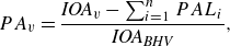
We plot the local, non-dimensional pressure profiles ( $p=P / \rho U^2$
) in the vicinity of the three valves (region enclosed by two boundaries laying at a streamwise distance of 2.5D and 4D from the inlet) at various cardiac instants during the deceleration, and project the fluid pressure on the surfaces of the valves’ leaflets (figure 5 for the TMHV, figure 6 for the BHV and figure 7 for the BMHV). For all the valves under consideration, we observe that with the decreasing inlet velocity during the systolic deceleration, the pressure in the central orificial region decreases with time (
$p=P / \rho U^2$
) in the vicinity of the three valves (region enclosed by two boundaries laying at a streamwise distance of 2.5D and 4D from the inlet) at various cardiac instants during the deceleration, and project the fluid pressure on the surfaces of the valves’ leaflets (figure 5 for the TMHV, figure 6 for the BHV and figure 7 for the BMHV). For all the valves under consideration, we observe that with the decreasing inlet velocity during the systolic deceleration, the pressure in the central orificial region decreases with time ( $0.28 \lt t/T \lt 0.35$
), however, it does not decrease in the sinuses at the same rate. For both TMHV (shown in figure 5) and the BHV (shown in figure 6), this difference in the local hemodynamics leads to the development of a higher pressure on the sinus-sides (referred as Ps) of their leaflets in comparison with their central flow-sides (referred as Pc) as the flow continues to decelerate. Augmented with the earlier discussed negative transvalvular pressure difference during the systolic deceleration phase of the cardiac cycle (figure 4
d), the difference of the pressure across the two sides of the leaflets creates a pressure force acting in the closing direction of each leaflet of the TMHV (figure 5) and BHV (figure 6), submitting to which, their leaflets start to close while there still exists forward flow in the domain. Additionally, it is important to note that the leaflets of the TMHV and the BHV close towards the centre (see figure 1), that is, in the direction of lowering pressure during the systolic deceleration, a feature which supports an early closure.
$0.28 \lt t/T \lt 0.35$
), however, it does not decrease in the sinuses at the same rate. For both TMHV (shown in figure 5) and the BHV (shown in figure 6), this difference in the local hemodynamics leads to the development of a higher pressure on the sinus-sides (referred as Ps) of their leaflets in comparison with their central flow-sides (referred as Pc) as the flow continues to decelerate. Augmented with the earlier discussed negative transvalvular pressure difference during the systolic deceleration phase of the cardiac cycle (figure 4
d), the difference of the pressure across the two sides of the leaflets creates a pressure force acting in the closing direction of each leaflet of the TMHV (figure 5) and BHV (figure 6), submitting to which, their leaflets start to close while there still exists forward flow in the domain. Additionally, it is important to note that the leaflets of the TMHV and the BHV close towards the centre (see figure 1), that is, in the direction of lowering pressure during the systolic deceleration, a feature which supports an early closure.
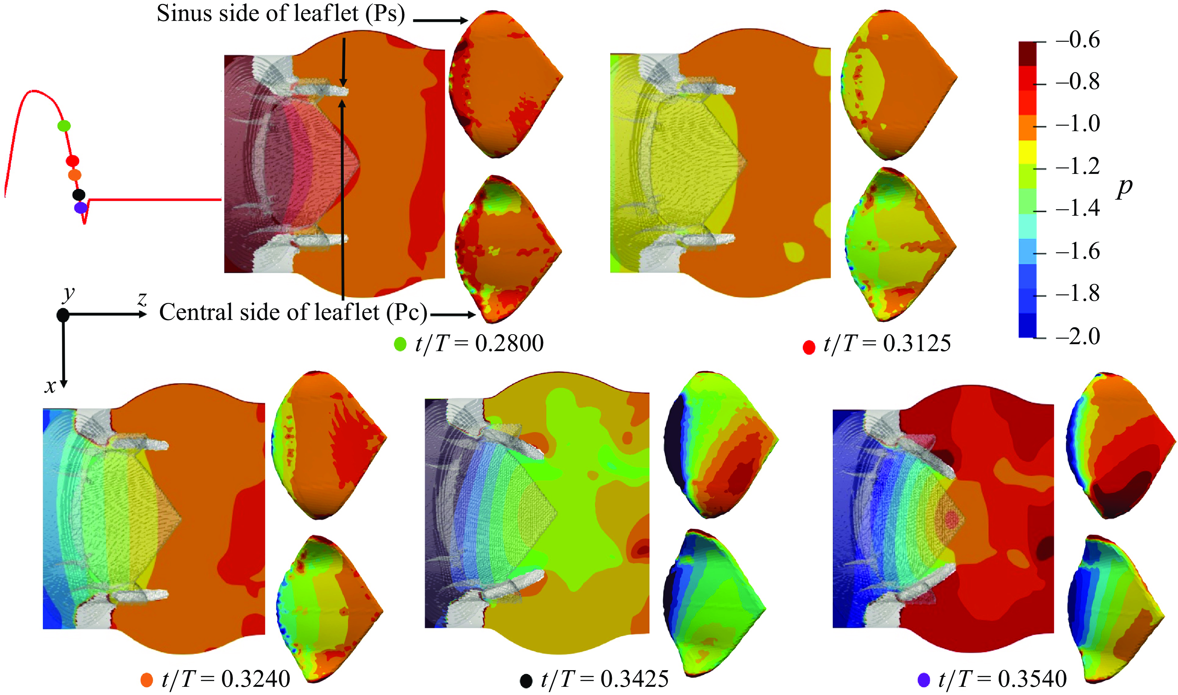
Figure 5. Local non-dimensional pressure variations in the vicinity of the TMHV.
In contrast to the TMHV and the BHV, the leaflets of the BMHV are located in the central orificial region itself, and thus the flow fields on their two sides are similar. Consequently, the pressure could be observed to be nearly the same on the sinus-sides (Ps) and central flow-sides (Pc) of the BMHV leaflets throughout the various instants of the systolic deceleration phase, as shown in figure 7. For this reason, the BMHV leaflets are unable to start their closing excursion until the onset of the reverse flow at the end of systole, which succeeds in creating a pressure force pointed in the direction of their fully closed position. It must be noted that even if the BMHV leaflets were oriented in a way that their sinus-sides could develop a higher pressure compared with their central flow-sides owing to the higher pressure in the sinus than the central orificial region during the systolic deceleration (figure 7), the fact that they close towards the sinuses, in the direction of the high pressure, would have certainly deterred an early BMHV closure.
As will be shown in what follows, the flow in the central orificial regions of the three valves undergoes a deceleration with the decreasing inlet velocity, consequently causing a pressure reduction in that region. The flow in the sinuses, however, does not undergo the same amount of deceleration owing to its characteristic, strong recirculation zones and as a result, demonstrates a higher pressure in comparison with the central orificial region.
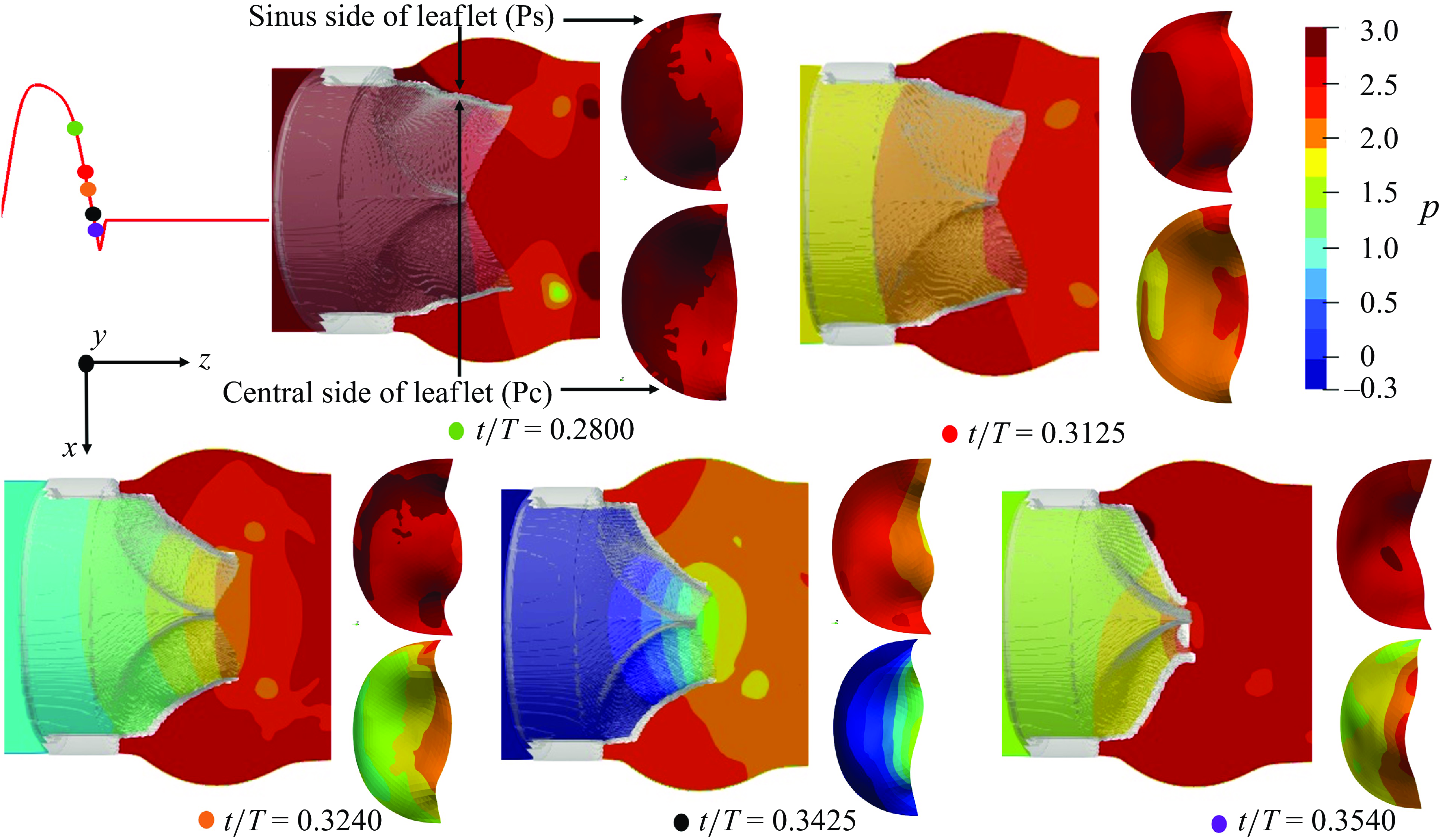
Figure 6. Local non-dimensional pressure variations in the vicinity of the BHV.
Figure 7. Local non-dimensional pressure variations in the vicinity of the BMHV.
3.3. Comparison of the velocity field and vorticity dynamics of the three valves
To further understand the closure behaviour of the valves’ leaflets in response to the cardiac flow, we obtain insights into their velocity field and the vorticity dynamics. Figure 8 presents a comparison of the x-planar velocity contours at various instants of the cardiac cycle for the three valves. By the early systolic phase (figure 8 a), the leaflets for the three valves could be observed to have completed their opening excursion, and the flow field starts to develop. At the peak systole, the flow field of the TMHV and the BHV could be observed to be mainly characterised by a strong, dominant central jet with a high velocity blood stream extending deep down the aortic region as shown by figure 8(b). The native aortic valve is also known to generate a flow profile dominated by a single central jet (Yoganathan et al. Reference Yoganathan, He and Casey Jones2004). The TMHV additionally demonstrates three narrow, lateral jets through the gaps between the fully opened leaflets and the valve’s housing, which are absent in the native valves or the BHV. For the BMHV, we observe three orificial jets with the two lateral jets being strong and wide in comparison with the narrow central jet, as previously observed by several studies (Dasi et al. Reference Dasi, Ge, Simon, Sotiropoulos and Yoganathan2007; Borazjani et al. Reference Borazjani, Ge and Sotiropoulos2010a ; Abbas et al. Reference Abbas, Nasif, Al-Waked and Said2020b ). A subtle observation from the hemodynamics of the two MHVs is that while the lateral jets in the TMHV are as strong as the BMHV, they are relatively much narrower compared with its central jet, and do not influence the pressure field, other than inducing a previously discussed small rebound of the TMHV leaflets during the valve’s opening phase. The direct evidence of this statement is illustrated by figure 5 for the cardiac deceleration, where the pressure in the regions covered by the lateral jets of the TMHV remain largely the same as the sinuses relative to the central orificial region. This indicates that the regions covered by the lateral jets and the recirculation zones in the sinus undergo a nearly similar amount of deceleration during late systole for the TMHV, being smaller than that in the central orificial region.
The wake region immediately downstream the BMHV is compounded with high and low velocity regions, in comparison with the TMHV and BHV, where the strong central jet washes away the valves’ downstream region with high velocity. As the cardiac cycle advances in time, the orificial jets for the three valves weaken and the flow decelerates during the late systolic phase (figure 8 c). By the start of the regurgitation flow, the velocity field is completely characterised by low velocity regions for the three valves as shown in figure 8(d).
It could be observed that the velocity profiles of the TMHV and the BHV look qualitatively similar in contrast to that of the BMHV during the early regurgitation, mainly because the leaflets of the later have covered little closure excursion at the onset of regurgitation. During the mid-diastolic phase (figure 8 e), small leakage flow could be observed to squeeze through the small openings in the apparently ‘fully closed’ valves, into the ventricle.
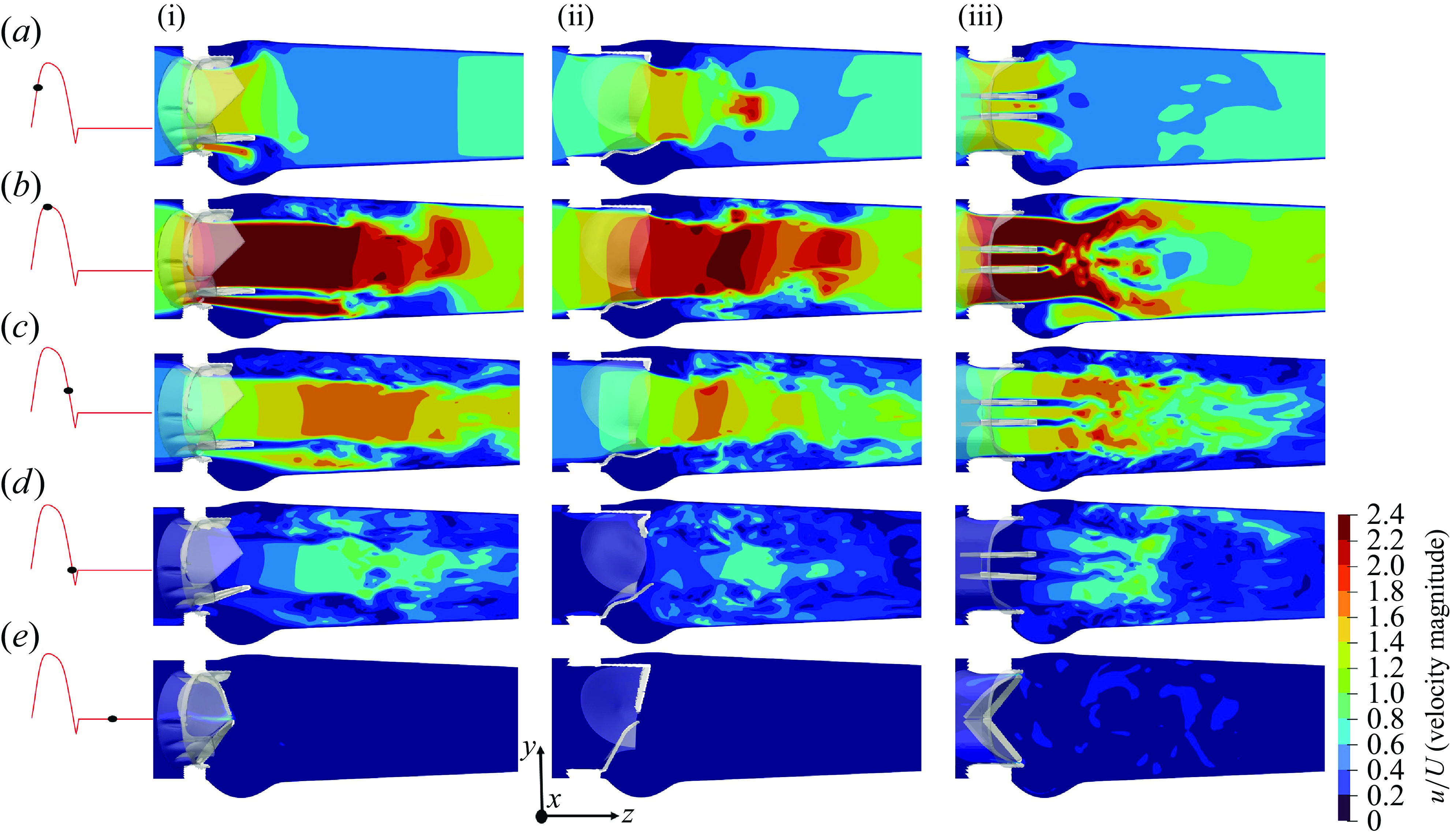
Figure 8. The x-planar view of the non-dimensional velocity field for TMHV (i), BHV (ii) and BMHV (iii); see Supplementary movie 2.
In the figure 9(a), the y-planar velocity profile at the peak systolic phase of the cardiac cycle for the three valves has been illustrated. The central jet for the TMHV extends to a streamwise distance (z/D) of 2.2 units, whereas that in the BHV extends to a z/D of 2.1 units, downstream of the aorta. On the other hand, the central jet in the BMHV is weak and extends to the extents of sinuses only before diffusing, to a z/D of 0.9 units. In figures 9(b) and 9(c), the velocity profiles for the three valves at the peak systole have been plotted over a line passing through the tip of their fully opened leaflets, along the arclengths x/D and y/D, respectively. The two ends of each arclength extend to the sinuses, and therefore capture the central jet, the lateral jets and the recirculation in the sinuses. Along the arclength x/D as observed in figure 9(b), the BMHV demonstrates the maximum velocity magnitude (u/U) of 2.610 in the central jet, being the highest in comparison with that of 2.525 in the TMHV and 2.200 in the BHV. The BMHV field also develops the highest u/U in the sinuses region along the arclength x/D, being a maximum of 0.739, in comparison with that of 0.666 in the TMHV and 0.115 in the BHV. Along the arclength y/D as observed in figure 9(c), the central jet of the BMHV demonstrates the maximum u/U of 2.622, being the highest in comparison with that of 2.520 in the TMHV and 2.210 in the BHV. The BMHV’s flow field has the highest u/U in the lateral jets, being a maximum of 2.600, in comparison with that of 2.520 in the TMHV and 0.0 in the BHV (no lateral jet) along the arclength y/D. It must be noted again, that the TMHV and the BHV generate a flow field which is dominantly characterised by a central jet along both arclengths, x/D and y/D, whereas the BMHV generates a qualitatively non-physiological field with a narrow central jet and two wide lateral jets.

Figure 9. (a) The y-planar view of the non-dimensional velocity field for the TMHV, the BHV and the BMHV at peak systole. (b) Non-dimensional velocity profile along the arclength x/D passing through the tip of the leaflets. (c) Non-dimensional velocity profile along the arclength y/D passing through the tip of the leaflets.

Figure 10. Cross-sectional velocity field (non-dimensional) at peak systole for the TMHV, the BHV and the BMHV.
The cross-sectional profile of the central jet for both, the TMHV and BHV at three different cross-sections (illustrated in figure 10 a as AA’, BB’ and CC’) is observed to be triangular (or star-like) in shape with three lobes for the peak systolic phase of the cardiac cycle as shown in figure 10(b). In contrast, the BMHV generates a weak central jet with a nearly rectangular cross-section, alongside two strong crescent-shaped lateral jets. The velocity profile on the cross-section BB’, which encompasses the aortic sinuses, demonstrates the highest velocity magnitudes in the sinuses under the BMHV flow. From the cross-section CC’, it could be qualitatively visualised that the central jet generated by the BMHV diffuses faster in comparison with those from the TMHV and the BHV, with the central jet almost diminishing in the BMHV by reaching the cross-section CC’. In figure 11, the contours of the streamwise velocities at the cross-section BB’ for the TMHV, the BHV and the BMHV have been plotted to visualise the flow recirculation in the sinuses, alongside the profiles of streamwise velocities plotted over three different lines across cross-section BB’, marked as line A, line B and line C, at peak systole. From the contours in figure 11, it could be observed that the BMHV field has the strongest localised flow recirculation zones in the sinuses. The line plots for arclength (y/D) along lines A, B and C show the highest adverse velocities in the sinuses for the BMHV among the three valves with a maximum adverse streamwise velocity (w/U) of −0.762, −1.133 and −0.680, respectively. For the TMHV, the maximum adverse w/U in the sinuses are −0.211, −0.076 and −0.243, along the lines A, B and C, respectively, whereas for the BHV, those are as low as -0.004, -0.012 and -0.016, respectively. The TMHV and the BHV shield the aortic sinuses due to the orientation of their fully opened leaflets in their respective housings during the peak systolic phase of the cardiac cycle, while the BMHV generates strong secondary flow with high adverse velocities in these regions, consequently resulting in the development of strong flow recirculation zones.
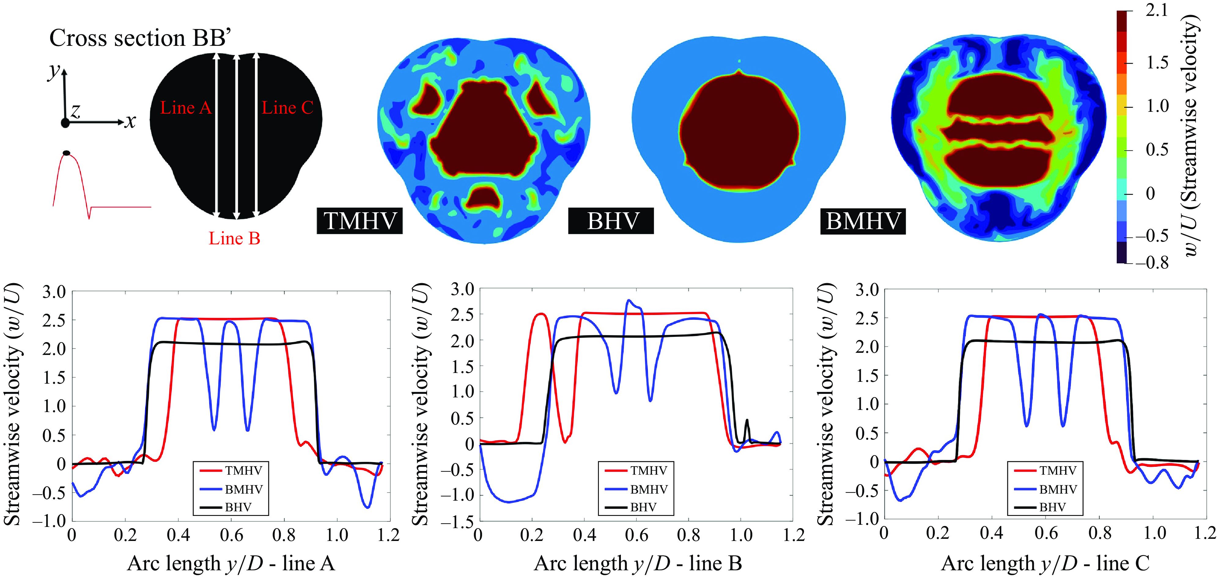
Figure 11. Cross-sectional streamwise velocity field at peak systole for the TMHV, the BHV and the BMHV alongside the line plots.
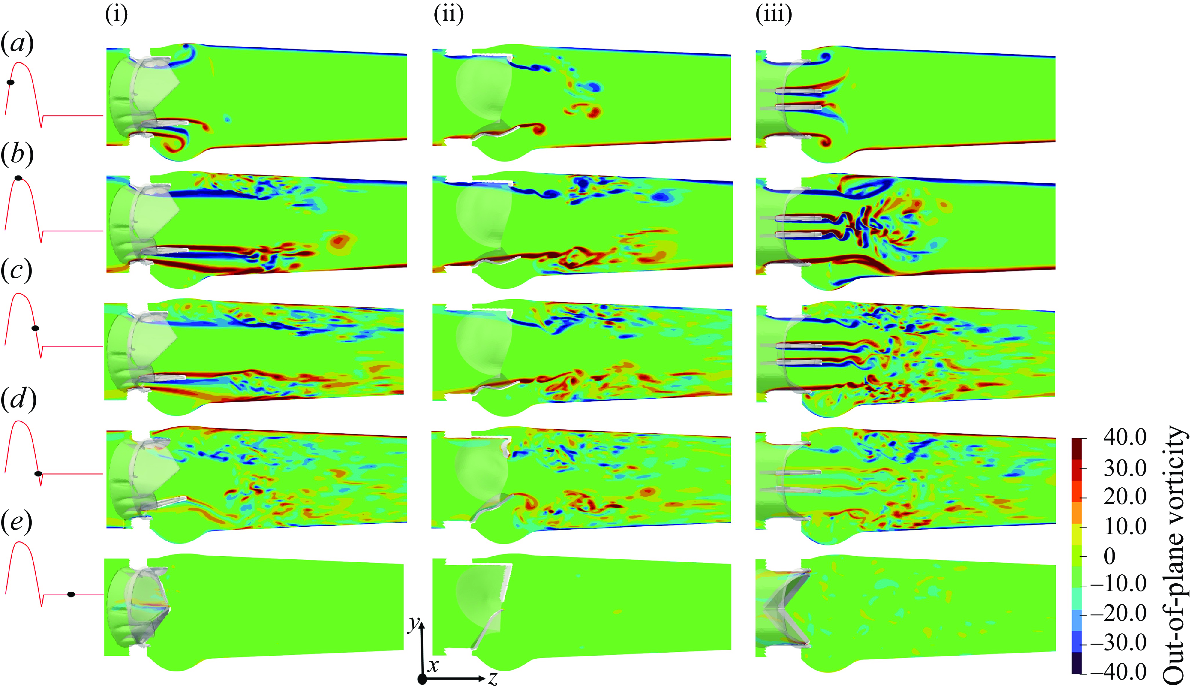
Figure 12. The x-planar view of the vorticity field for the TMHV (i), the BHV (ii) and the BMHV (iii).
The out-of-plane vorticity field for the three valves is illustrated in figure 12 on the x-plane for various instants of the cardiac cycle. The emanating shear layers could be broadly classified as those (i) corresponding to the lateral jets between the leaflets and valve’s housing in the TMHV and BMHV, which roll up into a ring-like structure expanding towards the sinuses and (ii) from the leaflets of the three valves, with each leaflet of the TMHV and BMHV producing two shear layers, being the outer layer (due to flow separation from the sinus-side) and the inner layer (due to flow separation from the central-side), whereas each leaflet of the BHV generates a single shear layer only due to the flow separation from the central-side as shown in figure 12(a) for the early systole. The vortex rings from the shear layers corresponding to the lateral jets of the TMHV and the BMHV move downstream the aorta as the inlet flow rate increases during the acceleration phase of the cardiac cycle, with the sinus vortex ring in the BMHV extracting a secondary layer of the sinus wall vorticity of opposite sign (figure 12 a,b). The shear layers from the leaflets of the TMHV and the BHV are found to be stable and coherent in the immediate wake of the valves by peak systole (figure 12 b), however, farther downstream of the aorta, a vortex ring separates from these shear layers, causing shedding that eventually destabilises the vorticity field. On the other hand, by peak systole, the two shear layers emanating from the leaflets of the BMHV get unstable and break down into small and chaotic von Kármán-like vortices. As the cardiac cycle advances in time (figure 12 c), the large-scale vortical structures weaken with the reduction in the incoming flow and gradually disappear, and a small-scale vorticity field dominates the wake of the three valves until late into the regurgitation phase (figure 12 d,e). Please refer to Appendix D for the description of the out-of-plane vorticity dynamics on the y-plane for the three valves.
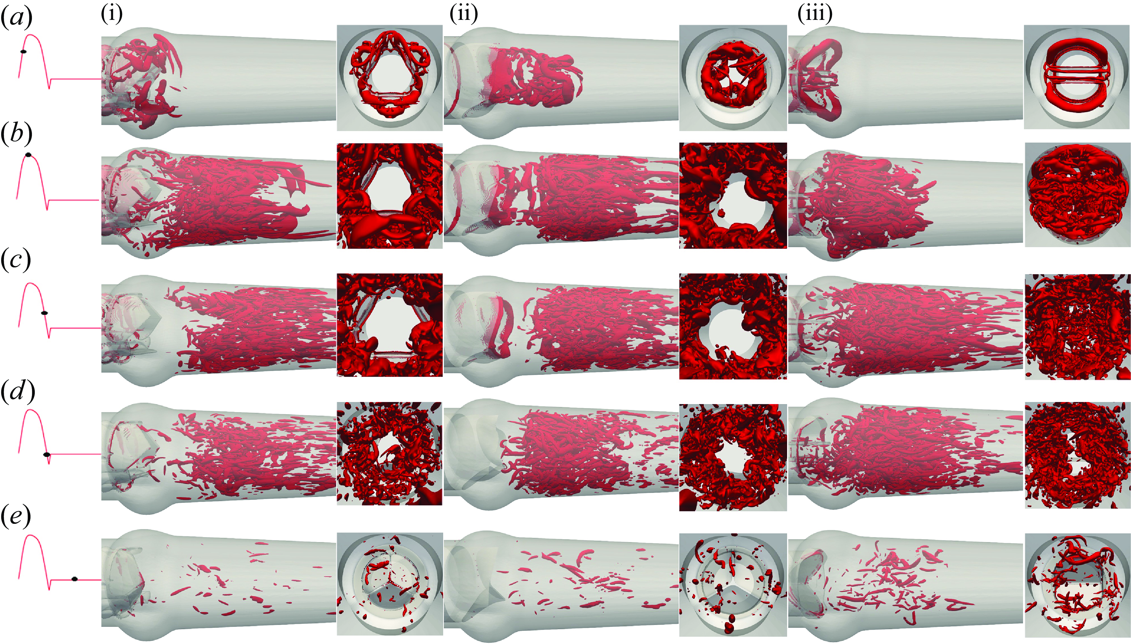
Figure 13. The 3-D vortical structures visualised by the isosurface of Q-criterion for the TMHV (i), the BHV (ii) and the BMHV (iii). See Supplementary movie 3.
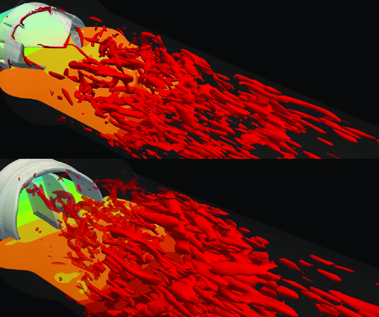
To further understand the vorticity dynamics of the three valves, we visualise the 3-D vortical structures by using the isosurfaces of the Q-criterion (Q = 90) in figure 13 at various cardiac instants. For each valve, the visualisations illustrate the isosurfaces of Q-criterion from two views (i) along the streamwise direction and (ii) perpendicular to the streamwise direction, captured from the downstream aorta. Figure 13(a) predominantly shows the development of the vortex ring from the shear layers corresponding to the lateral jets in the TMHV and the BMHV, whereas the free edges of the BHV emanate a complex vortical structure that moves downstream the aorta. At peak systole (figure 13 b), the central flow region of the TMHV and BHV is clearly void of vortices, whereas the shear layers from their leaflets shed vortices in the region near the wall of the downstream aorta past the sinuses. Although not observed from the 2-D (x-planar) out-of-plane vorticity field, we now observe vortices in the sinuses of the TMHV at peak systole (figure 13 b) from the shear layers corresponding to the lateral jets, which rapidly get washed away and the immediate wake regions of the TMHV and the BHV resemble each other, being void of vortices like the central flow region, during the systolic deceleration (figure 13 c) through early regurgitation (figure 13 d). In contrast, the inner and outer shear layers from the leaflets of the BMHV break down into chaotic vortices by peak systole (figure 13 b), thereby filling the aortic sinuses with vortices, and the immediate wake and the downstream aorta with a vortex street, which continue to dominate the BMHV’s flow field through the onset of regurgitation (figure 13 c,d). By mid-diastole, there exists myriads of randomly distributed and disorganised, weak vortices that lack a definite structure for all valves (figure 13 e).
From both, the out-of-plane vorticity field (figure 12) and the 3-D vortical structures (Q-criterion, figure 13), we observe that while the aortic sinuses are filled with vortices during the systole, these vortices are weak compared with those observed downstream the valves. During the systolic deceleration, the vortices in the sinuses further weaken in concord to those in the immediate wake of the valves and downstream the aorta, thereby not significantly influencing the flow field, specifically the pressure in the sinuses.
4. Discussion
In this research, 3-D numerical FSI simulations have been carried out to compute and compare the leaflet kinematics and the associated hemodynamics of a TMHV and a BMHV, with a BHV under similar conditions to identify the main reasons behind their closure dynamics. In what follows, we compare our observations with the previous work in the literature. Afterwards, we discuss the main reasons behind the early closure of BHV and TMHV relative to the BMHV, and state the assumptions/limitations of this work.
We employ the flow/velocity boundary conditions at the inlet of the domain, with the prescription of a transient cardiac pulse, instead of pressure inlet boundary conditions. Our results show that the leaflets of the TMHV and the BHV start to close during the late systolic deceleration phase of the cardiac cycle and complete most of their closing excursion by the early regurgitation, whereas the BMHV leaflets start to close with the onset of the regurgitation. These observations are consistent with the past experimental studies (Lu et al. Reference Lu, Liu, Huang, Lo, Lai and Hwang2004; Li et al. Reference Li, Chen, Lo and Lu2011; Vennemann et al. Reference Vennemann, Rösgen, Heinisch and Obrist2018). However, these studies observed that the BMHV leaflets close abruptly and much faster than the TMHV and the BHV. Indeed, several previous studies including some from our own research group reported that the BMHV leaflets close in less than 100 ms (Borazjani & Sotiropoulos Reference Borazjani and Sotiropoulos2010; Borazjani et al. Reference Borazjani, Ge and Sotiropoulos2010a ; Yun et al. Reference Yun, McElhinney, Arjunon, Mirabella, Aidun and Yoganathan2014b ; Abbas et al. Reference Abbas, Nasif, Al-Waked and Said2020b ). This disparity could be attributed to the prescription of a similar flow curve for the three valves despite the fact that the BMHVs are known to have higher retrograde flow relative to other artificial heart valves (Yoganathan et al. Reference Yoganathan, He and Casey Jones2004; Borazjani et al. Reference Borazjani, Ge and Sotiropoulos2010a ). The reduced retrograde velocity at the inlet boundary for the BMHV deterred its rapid closure in this study, indicating a trade-off between the simulations under similar conditions and previously observed closure kinematics of the BMHV. The reader is referred to Appendix E for a monologue on the dependence of the leaflet kinematics of the BMHV on the regurgitation volume, which demonstrates that the start to closure of the BMHV leaflets is independent of the regurgitation volume. Additionally, we assert that the conclusions drawn about the start of closure are not affected by the use of flow/velocity inlet instead of a pressure inlet approach since, during the systole, as illustrated by figure 4(d), the velocity and the pressure curves are highly correlated. The transvalvular pressure difference follows the acceleration and deceleration of the velocity curve. The differences associated with the use of these boundary conditions might prominently manifest themselves during the diastolic phase of the cardiac cycle when the same pressure boundary condition may create different retrograde flow.
Our simulated velocity fields and the vorticity dynamics of the TMHV, BMHV and BHV bear close resemblance with the past numerical and experimental studies and provide great help in understanding their respective pressure fields and closure behaviours. The flow in the TMHV and BHV is dominantly characterised by a strong central jet, being void of eddies, washing away the downstream wake region of the valves during the cardiac systole. The central jet from the two valves has been observed to have a triangular (or star-like) cross-sectional profile with three lobes, congruous with the findings of the past experimental studies with bioprosthetic (Hasler et al. Reference Hasler, Landolt and Obrist2016) and transcatheter trileaflet aortic valves (Pietrasanta et al. Reference Pietrasanta, Zheng, De Marinis, Hasler and Obrist2022). The shear layers bounding the central jets from the TMHV remain largely well-defined and coherent in the valve’s immediate wake as observed by Nitti et al. (Reference Nitti, De Cillis and de Tullio2022), similar to those from the BHV. On the other hand, the BMHV generates triorificial jets and the shear layers emanating from its leaflets break down into small and chaotic von-Kármán-like vortices by the peak systole as observed experimentally by Dasi et al. (Reference Dasi, Ge, Simon, Sotiropoulos and Yoganathan2007) and numerically by Borazjani et al. (Reference Borazjani, Ge and Sotiropoulos2008, Reference Borazjani, Ge and Sotiropoulos2010a ). Several features of the BMHV’s vorticity dynamics, such as the roll up of the shear layers from its housing into the sinus, extraction of the vorticity of opposite sign from the sinus wall, and a fast downstream travel of the leaflet shear layers than the one in the sinuses are in good agreement with experimental findings (Dasi et al. Reference Dasi, Ge, Simon, Sotiropoulos and Yoganathan2007).
While the main factor influencing the early closure of the TMHV and BHV, and the delayed closure of the BMHV could be hypothesised as the varying pressure field on the two sides of their leaflets (Borazjani et al. Reference Borazjani, Ge and Sotiropoulos2010a ), it has yet to be proven as the sole controller behind the closing behaviours of these valves. We observe that the leaflets of the artificial heart valves divide the flow domain into two parts: (i) the fast, forward flow central orificial region and (ii) the recirculation region in the sinuses, as observed in figure 11. With the flow deceleration, the pressure drops in the central orificial region, as it is primarily driven by the acceleration/deceleration of the incoming flow, directly evident from the Navier–Stokes equations if the viscous effects are ignored,
 \begin{equation} \frac {Du_i}{Dt}=-\displaystyle \frac {\partial\def\negativespace{} P}{\partial x_i}. \end{equation}
Conversely, the flow in the recirculation zones does not undergo the same amount of deceleration, causing a relatively higher pressure in the sinuses compared with the central orificial region. The flow deceleration in the discussed two regions can be qualitatively observed by the flow variations in these regions at different cardiac instants in figure 8. The compliance of the aorta typically increases the pressure in the sinuses relative to the central orifice region as demonstrated by a simplified, 1-D model for pressure variation in Appendix F. The utility of 1-D pressure modelling in aorta is not to be undermined, as such a model has been shown to efficiently capture the spatial pressure distribution on BHV leaflets with little deviation from a 3-D flow simulation, alongside an added advantage of huge computational efficacy (Chen & Luo Reference Chen and Luo2020).
Following the change in the local hemodynamics due to deceleration, a higher pressure is observed to develop on the sinus-sides of the leaflets of the TMHV and BHV than their central flow-sides during the deceleration phase, which preludes the closure kinematics of the two valves. The fact that the leaflets of the TMHV and BHV close towards the centre complements the resultant pressure force pointing towards the centre, in their closing direction, to enable a complete valve closure by early regurgitation. This finding remains intact even if the aortic compliance is taken into the account, as suggested by the pressure contours on the aortic and left-ventricular sides of an aortic valve modelled in a deforming aorta (Marom et al. Reference Marom, Haj-Ali, Raanani, Schäfers and Rosenfeld2012). The BMHV leaflets are, however, oriented in the central orificial region, and therefore the pressure on their sinus-sides and the central flow-sides has been observed to be practically the same during the systolic deceleration. In addition, the BMHV leaflets close towards the sinus, and thus even if they had a higher pressure on their sinus-sides, the resultant pressure force would act in the opposite direction of their closure, thereby inhibiting any excursion. For this reason, the BMHV leaflets wait for the reversal of the flow direction to start closure. The trend of the delayed BMHV closure is found to be independent of the cardiac cycle-to-cycle variations (refer to Appendix A). To the best of authors’ knowledge, this study for the first time manifests the spatial pressure distribution on the two sides of the leaflets of 3-D artificial heart valves, developed due to the decelerating flow, as the sole reason behind the valves’ closing behaviour, thereby proving the hypothesis put forth by Borazjani et al. (Reference Borazjani, Ge and Sotiropoulos2010a ). Granted the weakening of the vortices in the aortic sinuses by late systole, the authors find it unlikely that they might complement the adverse pressure gradient in the valve closure phase, by generating high pressure or viscous shear stresses in the aortic sinuses.
The preceding discussion implicitly views LV as a positive displacement pump driving a given volume (equal to the stroke volume) through the cardiovascular system (Le & Sotiropoulos Reference Le and Sotiropoulos2013; Song & Borazjani Reference Song and Borazjani2015; Verzicco Reference Verzicco2022). In this perspective, the pressure is a consequence of the resistance offered to the flow by the valves, the aorta and the rest of the system. The valves open and close due to the pressure created by the valve’s interaction with the flow. In another perspective, the LV could be considered as a battery that generates the potential difference (i.e. the pressure), causing the current (i.e. the flow of blood) to pass through a network of resistors and capacitors (i.e. the aortic valve, friction and elasticity) of the aorta (Liang & Liu Reference Liang and Liu2005; Westerhof et al. Reference Westerhof, Lankhaar and Westerhof2009; Barrett et al. Reference Barrett, Brown, Smith, Woodward, Vavalle, Kheradvar, Griffith and Fogelson2023). In this perspective, the valves open and close directly in response to the pressure difference between the LV and the aorta. Nevertheless, this perspective (pressure difference generates the flow) alone cannot explain the early closure of BHV and TMHV compared with the BMHV because the pressure difference is the same across all these valves. In fact, based on our results (figure 4
d), the transvalvular pressure difference across the valve decreases at a faster rate (i.e. is more negative) for the BMHV than TMHV and BHV during the systolic deceleration. Our use of velocity/flow boundary conditions suggest the employment of the first perspective in our work. Nevertheless, we argue that our explanation remains valid even with the second perspective (pressure boundary conditions). This is best explained by the simple model in Appendix F, in which the pressure in the sinus and central region are related to the pressure downstream in the aorta ( $P_L$
in Appendix F). It shows that given a pressure downstream of the valve (pressure boundary condition as in the first perspective), the pressure in the sinus will be higher than that in the central jet region due to the lower deceleration in the sinus.
$P_L$
in Appendix F). It shows that given a pressure downstream of the valve (pressure boundary condition as in the first perspective), the pressure in the sinus will be higher than that in the central jet region due to the lower deceleration in the sinus.
The main assumptions/limitations of this work include thefollowing. (i) Employment of a simplified aorta without modelling its anatomic curvature, as previously done by several studies, both in vitro (Dasi et al. Reference Dasi, Ge, Simon, Sotiropoulos and Yoganathan2007; Jahren et al. Reference Jahren, Winkler, Heinisch, Wirz, Carrel and Obrist2017; Ferrari & Obrist Reference Ferrari and Obrist2024) and in silico (Hedayat et al. Reference Hedayat, Asgharzadeh and Borazjani2017; Abbas et al. Reference Abbas, Nasif, Al-Waked and Said2020b ; Chen & Luo Reference Chen and Luo2020). In a previous study by our research group (Borazjani et al. Reference Borazjani, Ge and Sotiropoulos2010a ), while it was observed that the curvature of the anatomic aorta affects the leaflet kinematics and the overall hemodynamics of a BMHV relative to a straight aorta without curvature, the initiation of the BMHV closure remained unchanged between a straight and anatomic aorta, i.e. the leaflets started to close after the onset of regurgitation. (ii) Use of a simplified inlet geometry instead of the LV–aorta configuration, similar to several studies investigating the leaflet kinematics and hemodynamics of artificial heart valves, both in vitro (Haya & Tavoularis Reference Haya and Tavoularis2017; Bellofiore et al. Reference Bellofiore, Donohue and Quinlan2011) and in silico (Borazjani & Sotiropoulos Reference Borazjani and Sotiropoulos2010; Abbas et al. Reference Abbas, Nasif, Al-Waked and Said2020a ; Zolfaghari et al. Reference Zolfaghari, Kerswell, Obrist and Schmid2022; Asadi & Borazjani Reference Asadi and Borazjani2023; Bornemann & Obrist Reference Bornemann and Obrist2024). Le & Sotiropoulos (Reference Le and Sotiropoulos2013) developed a realistic model of the contraction/relaxation of the LV and carried out numerical simulations of a BMHV implanted in an anatomic aorta. Other than observing the differences in the vorticity dynamics of the BMHV, they also reported highly asymmetric leaflet kinematics during the valve’s closure phase in their simulations relative to the pulsatile flow-driven simulations. Asadi et al. (Reference Asadi, Hedayat and Borazjani2022) reported that when the LV motion is modelled instead of prescribing an inflow, the high asymmetry in the closure dynamics of a BMHV renders it difficult to suggest a preferred valve orientation in terms of symmetric closing and minimum rebound of BMHV leaflets after an initial closure. Annerel et al. (Reference Annerel, Degroote, Claessens, Segers, Verdonck and Vierendeels2012) reported that orientation of the LV with respect to the valve, being symmetric or asymmetric, can also influence the opening kinematics of a BMHV leaflet. We maintain that modelling a LV–aorta configuration might cause striking differences in the leaflet kinematics when compared with modelling with a prescribed pulsatile inflow, however, a review of past studies establishes that the BMHV leaflets start to close due to flow reversal, withstanding the modelling strategy. (iii) Use of a rigid aorta, which as discussed in Appendix F does not affect the conclusions of this work, contingent on the fact that the uncertainty in material properties of the aorta will add additional questions to the problem. Furthermore, the compliance of the arteries does not significantly affect the pressure waveform but mainly affects the phase difference between the flow and the pressure waveforms. (iv) Application of the same inlet flow curve for different valves (as discussed above in detail), despite the established fact that all valves have a different closure volume associated with them. Perhaps the application of a Dirichlet pressure boundary condition for the diastolic phase of the cardiac cycle might aid in a better estimation of the regurgitant volume for each valve. However, the current simulations employ the pressure-correction projection method with an assumption of modelling the blood as incompressible fluid, for which as discussed earlier in § 2, the prescription of Dirichlet pressure boundary conditions may result in reduced convergence rates and could be numerically cumbersome. Instead, adding a forcing term, representing the driving pressure gradient, to the right-hand side of momentum equations might be an alternative to drive the flow without applying flow boundary conditions. (v) Incorporation of a small gap between the leaflets when they are realistically fully closed, which is necessary to maintain a simply connected upstream and downstream domain of the valves, thereby enabling the convergence of the pressure-Poisson solver. The limitations (iv) and (v) together cause the generation of a lower transvalvular pressure difference compared with the physiologic pressure difference during diastole (figure 4 d). The low pressure difference during diastole, notwithstanding, does not affect the conclusions related to start of valve closure during late systole for the TMHV and BHV, while at the brink of regurgitation for the BMHV. The independence of the drawn conclusions is further elaborated in the appendices, as earlier cited in the manuscript.
5. Conclusion
In this research, we investigated the closure dynamics of heart valves by comparing the leaflet kinematics and hemodynamics of the trileaflet and bileaflet designs of MHVs against a BHV. It was observed that in response to the cardiac flow, the leaflets of the TMHV open synchronously, do not flutter when fully opened, start to close during mid-deceleration and completely close in a slightly asynchronous fashion by the early regurgitation, similar to the BHV. When fully opened, the hemodynamics of the TMHV were also observed to be similar to that of the BHV, dominated by a strong central jet with a ‘star-like’ cross-section, in contrast to the BMHV which generates non-physiological triorificial blood flow, with the two lateral jets being stronger and wider than the narrow central jet.
The closure of the TMHV and the BHV is shown to be initiated by a pressure force pointing towards the closing direction of their leaflets, developed due to a higher pressure on the sinus-sides of the their leaflets in comparison with their central flow-sides (refer to figure 5 for the TMHV, and figure 6 for the BHV). The lower pressure in their central lumen is shown by a simple model (Appendix F that relates pressure to the acceleration through (F2)) to be due to the forward flow deceleration of their central jets, which undergo a higher amount of deceleration relative to the flow in the sinuses, congruous to as observed in figure 5 for the TMHV and figure 6 for the BHV. For the BMHV, the triple orificial jets also undergo a higher amount of deceleration relative to the flow in the sinuses as observed in figure 7. However, the pressure on the sinus-side and the central flow-side of the BMHV leaflets is found to be nearly the same (figure 7) as also predicted by the simple model (Appendix F) to be due to the similar deceleration of the jets on either side of the leaflets. In addition, note that the higher pressure on the sinus-side of the leaflets will prohibit the closure of the BMHV because of its designed closure mechanism (i.e. a closure towards the sinus, as shown in figure 1). The BMHV leaflets, therefore, have to wait for the onset of regurgitation to start their closure kinematics. The vortices in the aortic sinuses, first postulated by Bellhouse & Talbot (Reference Bellhouse and Talbot1969) as an important contributor to the valve closure mechanism, are unlikely to interact with the adverse pressure gradient and promote the valves’ closure as they are observed to have lost their strength by the systolic deceleration phase.
Based on the above discussion of the TMHV and the BMHV, the design principles to ensure an early closure of the MHVs could be (i) generation of a strong central jet relative to the lateral jets, as it will cause the development of a lower pressure in the central orificial region compared with the sinuses during systolic deceleration, (ii) a valve closure direction towards the centre rather the sinuses, which will augment the pressure force pointed towards the low pressure region to drive the leaflets towards the centre, which is, a complete closure before the left ventricular expansion.
Supplementary movies
Supplementary movies are availabe at https://doi.org/10.1017/jfm.2025.354.
Acknowledgements
The authors gratefully acknowledge the financial support and provision of the TMHV’s geometric model from Novostia, Switzerland, and computational resources from the High-Performance Research Computing (HPRC) Center at Texas A&M University, College Station, Texas, USA. The authors are thankful to Dr D. Obrist (ARTORG Center, University of Bern) for the provision of the cardiac flow rate. In addition, the authors thank Mr C. Nemoz, Verification and Validation Manager at Novostia, Switzerland for his valuable suggestions on the research results and the manuscript.
Funding
This work was partly supported by Novostia, Switzerland.
Declaration of interests
I.B. has received grants from the company, Novostia, Switzerland.
Appendix A. Cycle to cycle variations analysis
Past experimental studies investigating the blood flow through artificial heart valves have reported a strong dependence of the obtained results on the cardiac cycle-to-cycle variations (Dasi et al. Reference Dasi, Ge, Simon, Sotiropoulos and Yoganathan2007; Li et al. Reference Li, Chen, Lo and Lu2011). The initial conditions for each cardiac cycle may vary, which can eventually influence the numerical results. To investigate the cardiac cycle-to-cycle variations, we simulated four cardiac cycles for the BMHV, and compared their results in terms of leaflet kinematics and velocity profiles at various instants.
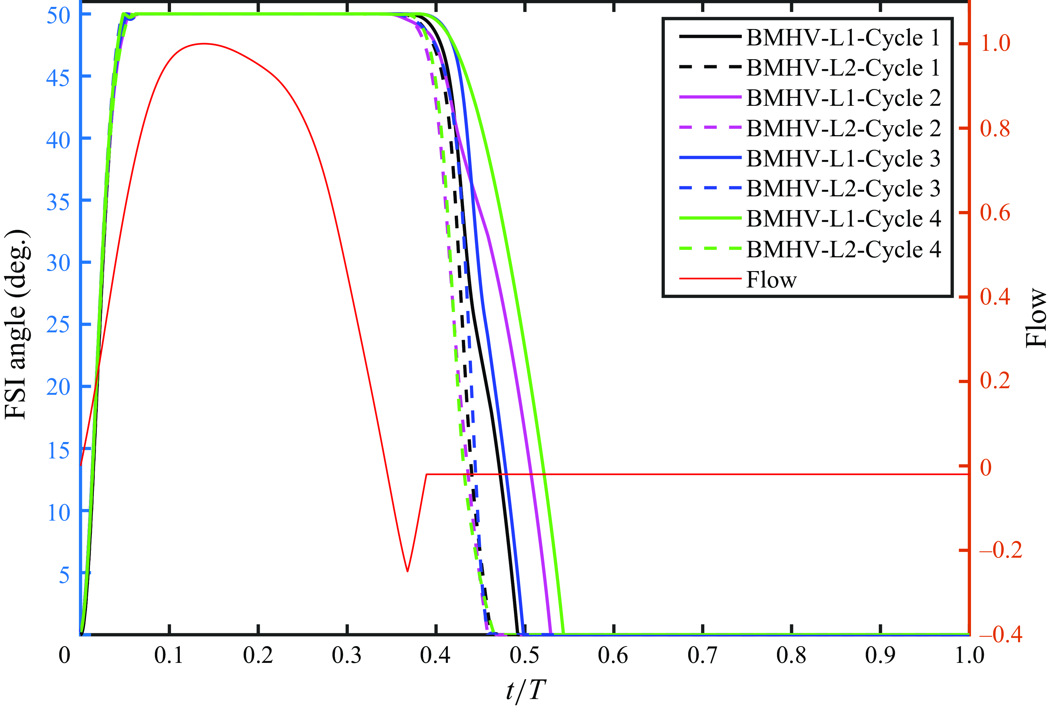
Figure 14. Leaflets kinematics for various cardiac cycles with a BMHV.
As shown by figure 14, while the opening kinematics of the BMHV leaflets for all cardiac cycles are in good agreement, the closing phase shows strong cycle-to-cycle variations as observed in past experimental studies. These cycle-to-cycle variations, notwithstanding, will not affect the conclusions because the leaflets of the BMHV start to close after the onset of regurgitation for all cycles. Furthermore, Leaflet 2 closes earlier in time compared with Leaflet 1 in all cycles. In summary, same trends are observed in all cycles and the start of closure is not affected by the cycle-to-cycle variations.
The velocity profiles might manifest themselves as a relatively more robust parameter to perform a cardiac cycle-to-cycle variations analysis, compared with the leaflet kinematics. As figures 15 and 16 show, the velocity contours and profiles plotted at a line located on a streamwise distance of 0.05D from the tip of the fully opened BMHV leaflets at several cardiac instants demonstrate similar patterns and magnitudes for the second, third and the fourth cardiac cycle, in comparison with that from the first cardiac cycle.
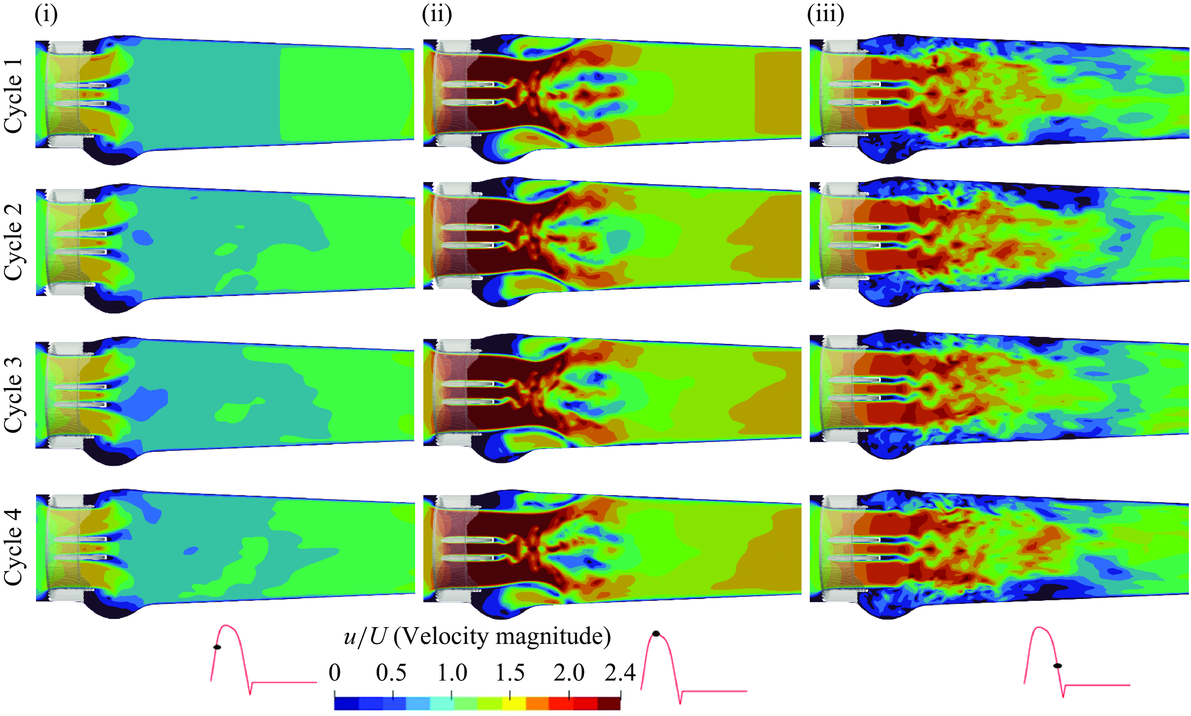
Figure 15. Velocity contours at several instants during multiple cardiac cycles for a BMHV: early systole (i), peak systole (ii) and late systole (iii).
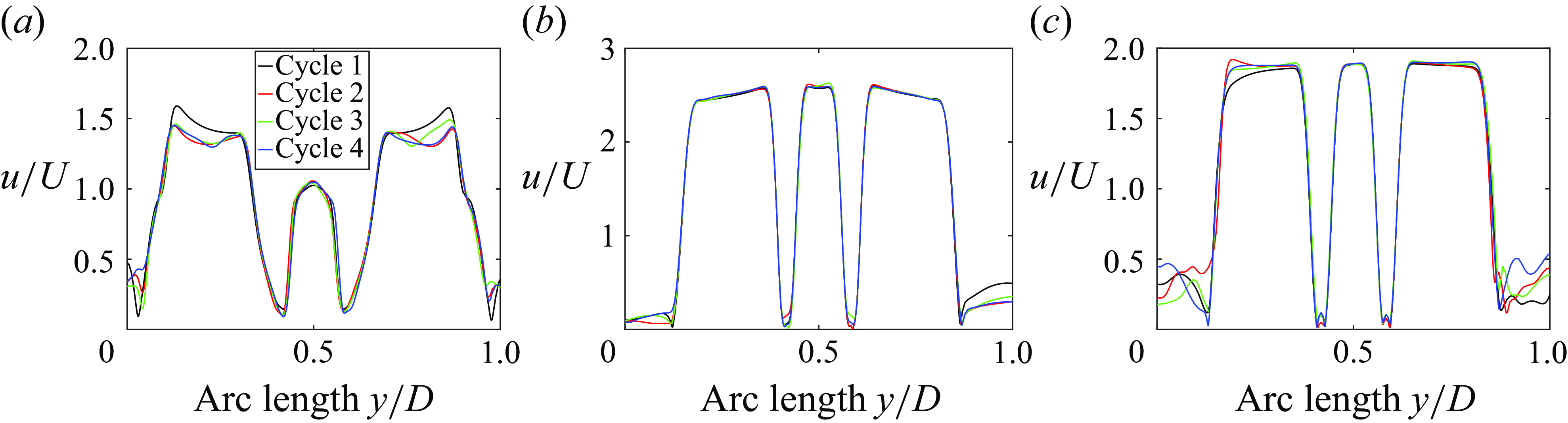
Figure 16. Plots of the BMHV velocity profiles along an arclength for various instants of the cardiac cycles (a) early systole, (b) peak systole and (c) late systole.
It is important to note that while the numerical simulations are highly resolved, they are computationally expensive. One cardiac cycle requires around a week of simulation time when being executed on eight distributed memory nodes with 48 cores on each of them, i.e. on 384 cores. Considering that the opening of the valve and the general flow features are consistent after the second cycle, we have presented the results from the second cardiac cycle for each valve in this manuscript.
Appendix B. Time step independence
A time step independence study was carried out by comparing the velocity contours and profiles of the TMHV (plotted at a line located on a streamwise distance of 0.05D from the tip of the fully opened leaflets) for two non-dimensional time step sizes of 0.005 and 0.0025.
It is worth mentioning that the cardiac cycle comprises of 0.85714 s (with a heart rate of 70 beats per minute), or in the non-dimensional form as demonstrated by
 \begin{equation} T^*=T/(D/U)=0.85714/(0.02582/0.6548)=21.73722, \end{equation}
where $T^*$
is the non-dimensional time.
$T^*$
is the non-dimensional time.
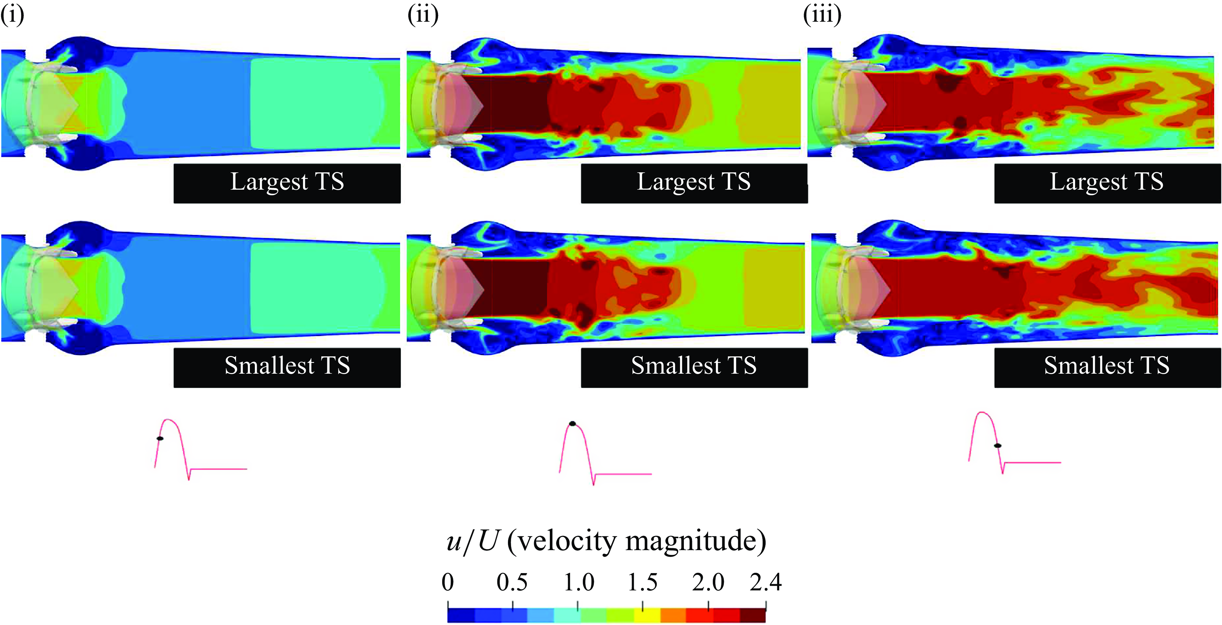
Figure 17. Velocity contours at several cardiac instants for a TMHV, obtained from two time steps of different sizes: early systole (i), peak systole (ii) and late systole (iii).
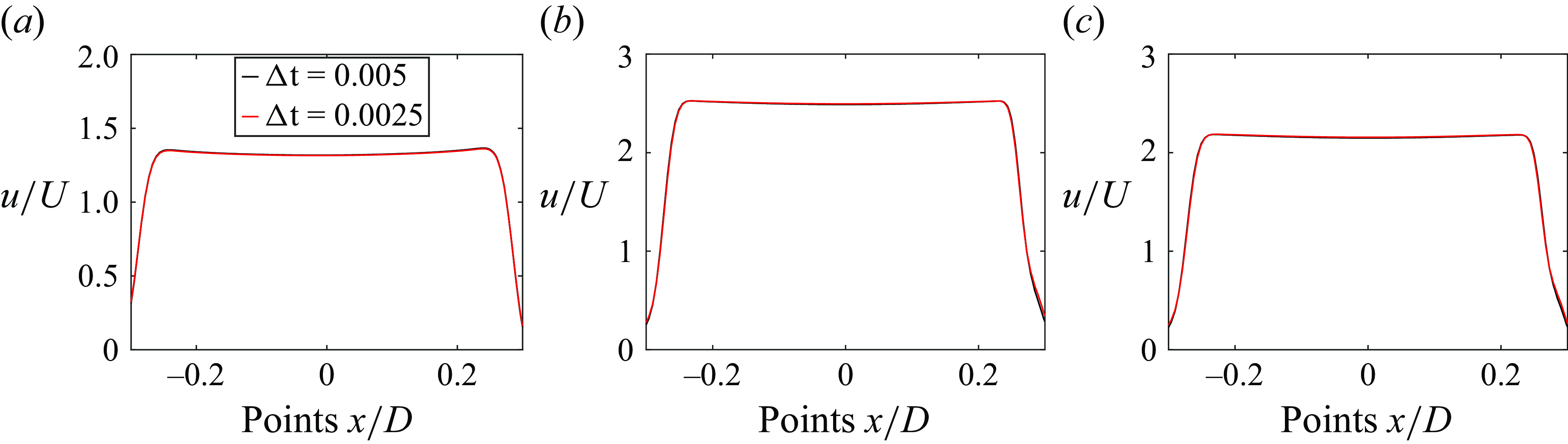
Figure 18. Plots of the velocity profiles at several cardiac instants for a TMHV, obtained from two time steps of different sizes: (a) early systole, (b) peak systole and (c) late systole.
Thus, the time step size of 0.005 corresponds to a total number of 4350 time steps needed for the discretisation of the complete cardiac cycle, while that of 0.0025 corresponds to a total number of 8700 time steps. We have referred to the time step size of 0.005 as the ‘largest TS’ and time step size of 0.0025 as the ‘smallest TS’ in figure 17.
As shown by the figures 17 and 18 for the early systole, the peak systole and the late systolic instants of the cardiac cycle, the velocity profiles demonstrate a good agreement for the two time steps, and fractionally differ by less than 1 %.
It could therefore be established that the obtained numerical results are independent of the size of the time step. We thus carried out the further simulations and presented the results (in the manuscript) with the time step of the larger size (0.005) for all the valves.
Appendix C. Structural deformations of the BHV
In § 3, we could present the leaflet kinematics of the two MHVs as a graphical plot (figure 4 a) since they are rigid immersed bodies. However, such a plot could not be obtained for a BHV since its leaflets continuously deform during their elastic excursion, and therefore as mentioned before, we opted to compare the leaflet kinematics of the three valves by comparing their projected areas. The Supplementary movie 1 presents the 3-D transient leaflet kinematics of the three valves as visualised from the second cardiac cycle. In this appendix, we investigate the deformation of the BHV leaflets in response to the cardiac plug flow by colouring them with their non-dimensional displacement as illustrated by figure 19. It is worth reiterating that this study employs the recently developed and validated contact model of Asadi & Borazjani (Reference Asadi and Borazjani2023) for the BHV simulations.
During the opening phase of the BHV, when the cardiac flow is accelerating, we observe that the belly region of the leaflets, which is free to move in contrast to the fixed edges, exhibit high displacement relatively (figure 19
a). By peak systole (figure 19
b), the complete belly regions of the three leaflets show high displacement, which slightly continues to increase as the leaflets’ free edges undergo opening and fluttering motion after the peak systole (refer to Supplementary movie 4). The leaflets stay fully opened during the early deceleration phase of the cardiac cycle as could be observed from figure 19(c). During the late systolic deceleration (figure 19
d), the leaflets could be observed to have started their closure dynamics (as previously also demonstrated by the transiently reducing projected area in figure 4
b), and we observe high displacement regions getting concentrated near the free edges of the BHV leaflets compared with other parts of the leaflets through early regurgitation (figure 19
e). The leaflets fully close before t/T $\approx$
0.4, and hence we do not observe any displacement during diastole (figure 19
f) with the constant regurgitation prescribed at the inlet of the computational domain.
$\approx$
0.4, and hence we do not observe any displacement during diastole (figure 19
f) with the constant regurgitation prescribed at the inlet of the computational domain.
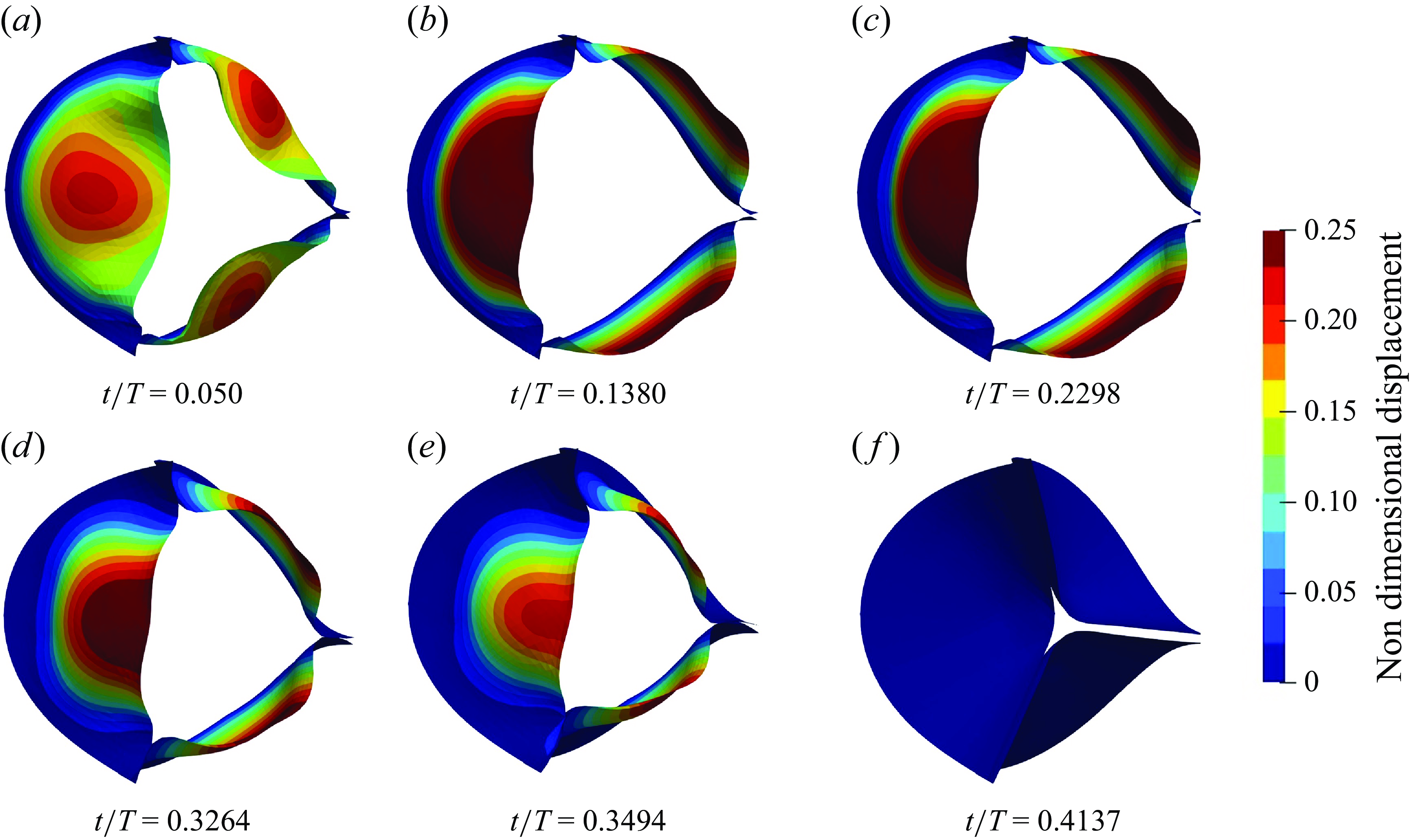
Figure 19. Transient deformation of the BHV, coloured by displacement at various instants of the cardiac cycle. See Supplementary movie 4.
Appendix D. Out-of-plane vorticity dynamics on the y-plane
In this appendix, we present the out-of-plane vorticity on the y-plane for the TMHV, the BHV and the BMHV. While most of the vorticity features are similar to those earlier observed in the x-planar view (figure 12), figure 20 clearly illustrates that the sinuses of the TMHV and the BMHV develop vortices during systolic acceleration (figure 20 b). The sinus vortices are negligibly weak in the BHV relative to those in its downstream wake. With the advancement in the cardiac cycle (figure 20 c,d), the vortices in the sinuses further weaken and eventually diminish in response to the decelerating flow. Consequently, the vortices in the sinuses do not significantly influence the pressure field. As a result, the adverse pressure gradient due to systolic deceleration is able to develop a higher pressure in the aortic sinuses compared with the central orificial regions of the three valves.
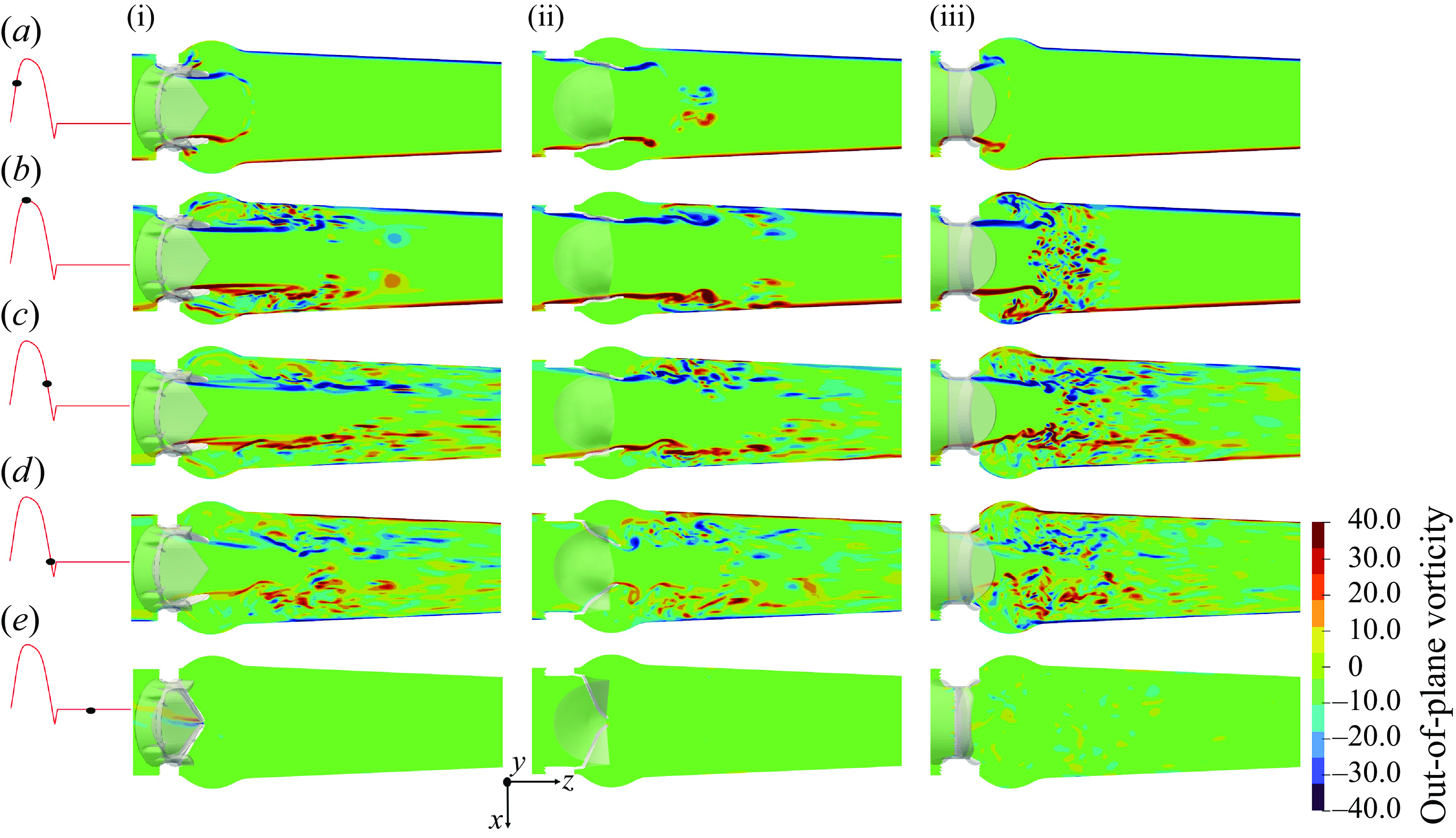
Figure 20. The y-planar view of the vorticity field for the TMHV (i), the BHV (ii) and the BMHV (iii).
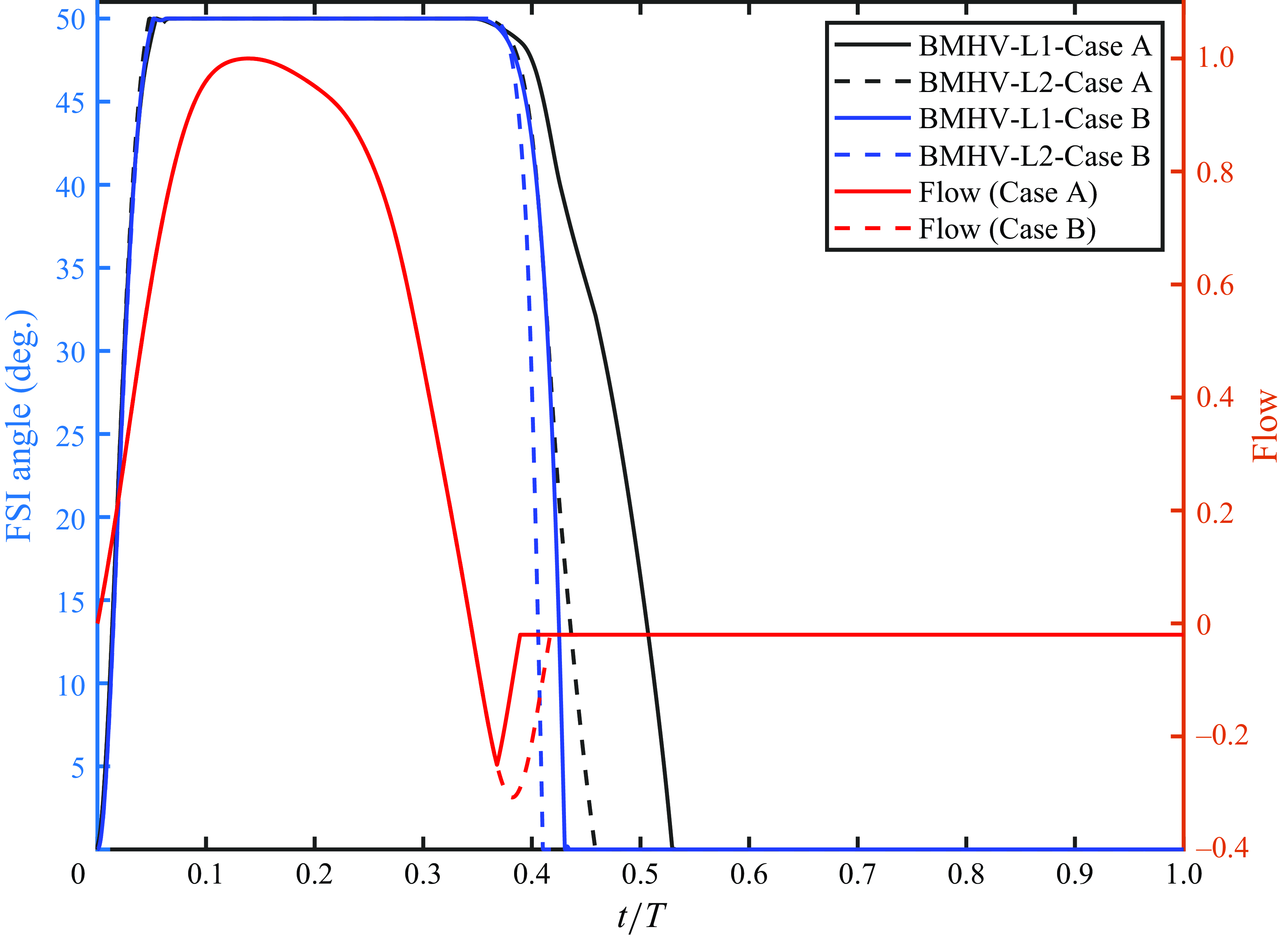
Figure 21. Variation in the leaflet kinematics of the BMHV with the regurgitation flow. Here L1 and L2 refers to Leaflet 1 and Leaflet 2 of the BMHV, respectively.
Appendix E. Dependence of the kinematics of BMHV leaflets on regurgitation
It is known that BMHVs have higher regurgitant volume than TMHV and BHV (Li et al. Reference Li, Chen, Lo and Lu2011; Vennemann et al. Reference Vennemann, Rösgen, Heinisch and Obrist2018) as discussed in the Introduction (§ 1) of the manuscript, however, a similar flow curve was chosen in this work for all the valves to ensure a comparison under similar flow conditions. To investigate the validity of this assumption, in this appendix, the variation in the closure kinematics of the BMHV leaflets with respect to the regurgitation flow is investigated. Figure 21 shows the leaflet kinematics for two cases with different flow curves, where Case A refers to the employment of the flow rate used as an inlet boundary condition in this study while Case B refers to that with a relatively higher regurgitation volume. A rapid and smooth closing of the BMHV leaflets is observed for Case B, with both leaflets taking less than 100 ms to fully close from a fully opened position. Nevertheless, the start of closure for Case A is identical to the Case B. This finding supports the previously drawn conclusions for the ’start to closure’ of the BMHV leaflets and demonstrates that they are not sensitive to the regurgitant volume, i.e. the two leaflets start their closure excursion at the onset of flow regurgitation.
Appendix F. One-dimensional model for pressure variation in compliant aorta
In this appendix, we employ a simplified 1-D analytical model to investigate the variations of pressure in the sinus and the central jet during closure for both rigid and compliant aorta. With reference to figure 22, the pressure $P_{L}$
at an arbitrary point located downstream the aorta is estimated by using the Windkessel model based on the flow rate
$P_{L}$
at an arbitrary point located downstream the aorta is estimated by using the Windkessel model based on the flow rate $Q(t)$
, compliance
$Q(t)$
, compliance $C$
and resistance
$C$
and resistance $R$
of the aorta, and initial systolic pressure at the moment when the valve opens
$R$
of the aorta, and initial systolic pressure at the moment when the valve opens $p_0$
(Fung Reference Fung2013):
$p_0$
(Fung Reference Fung2013):
 \begin{equation} P_L(t)=e^{-t/(RC)} \int _0^t \frac {1}{C} Q(t) e^{\tau /(RC)} {\rm d}\tau + p_0 e^{-t/(RC)}. \end{equation}
Note that for a rigid aorta, the relation between pressure at flow rate reduces to $P_L(t)=R Q(t)$
.
$P_L(t)=R Q(t)$
.
We tend to estimate the pressure in the sinus ( $P_s$
) and the central region (
$P_s$
) and the central region ( $P_c$
) by using the 1-D conservation of mass and momentum. From the conservation of momentum, we have
$P_c$
) by using the 1-D conservation of mass and momentum. From the conservation of momentum, we have
 \begin{equation} \displaystyle \frac {\partial u}{\partial t}+u\displaystyle \frac {\partial u}{\partial x}+\displaystyle \frac {1}{\rho }\displaystyle \frac {\partial P}{\partial x}=0 ,\end{equation}
whereas the continuity equation could be written as
 \begin{equation} \displaystyle \frac {\partial A}{\partial t}+\displaystyle \frac {\partial uA}{\partial x}=0 \Rightarrow \displaystyle \frac {\partial u}{\partial x}=\displaystyle \frac {1}{A} \left [-\displaystyle \frac {\partial A}{\partial t}-u\displaystyle \frac {\partial A}{\partial x} \right ] ,\end{equation}
where A is the area of any plane $k$
perpendicular to the streamwise direction and
$k$
perpendicular to the streamwise direction and $u$
is the streamwise velocity.
$u$
is the streamwise velocity.
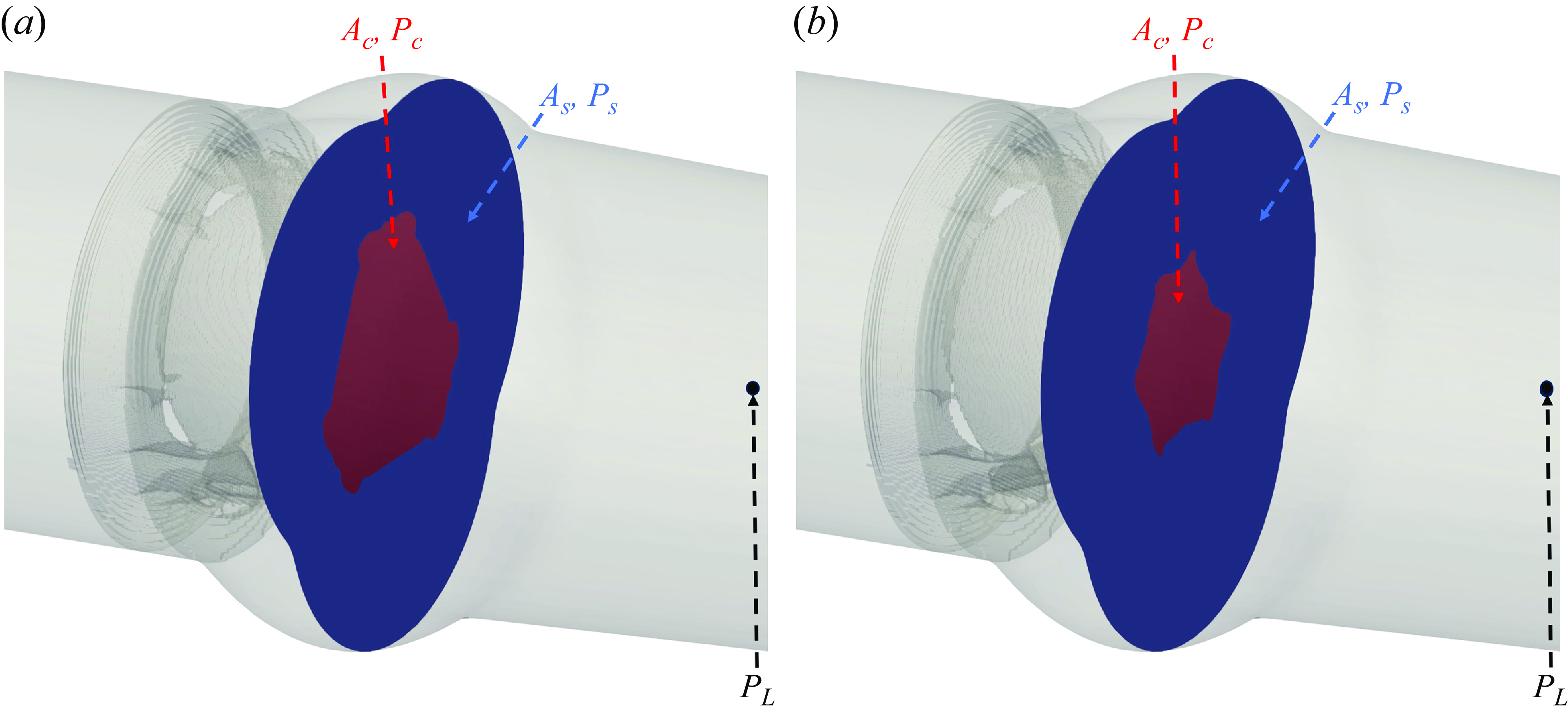
Figure 22. (a) Demonstration of the central orificial and the sinus areas when the leaflets of artificial heart valves are fully open. (b) Reduction in the central orificial area as the leaflets move towards their fully closed positions.
In the above equation, assuming that leaflets are almost parallel to the flow at the initiation of the closure, the variation of $A$
in space, i.e.
$A$
in space, i.e. $\partial A / \partial x$
is ignored relative to its variation in time. Replacing (F3) in (F2) and rearranging, while ignoring
$\partial A / \partial x$
is ignored relative to its variation in time. Replacing (F3) in (F2) and rearranging, while ignoring $\partial A / \partial x$
, we obtain
$\partial A / \partial x$
, we obtain
 \begin{equation} \frac {\partial u}{\partial t}-\frac {u}{A} \frac {\partial A}{\partial t} =-\frac {1}{\rho }\displaystyle \frac {\partial P}{\partial x} .\end{equation}
For the determination of the sinus and central pressures $P_{s}$
and
$P_{s}$
and $P_c$
, (F4) is integrated in
$P_c$
, (F4) is integrated in $x$
from point
$x$
from point $s$
or
$s$
or $c$
to point
$c$
to point $L$
:
$L$
:
 \begin{equation} P_{s}=P_{L}+\rho \int _s^L \displaystyle \frac {\partial u_{s}}{\partial t}{\rm d}x - \rho \int _s^L\displaystyle \frac {u_{s}}{A_s} \displaystyle \frac {\partial A_{s}}{\partial t} {\rm d}x, \end{equation}
 \begin{equation} P_{c}=P_{L}+\rho \int _c^L \displaystyle \frac {\partial u_{c}}{\partial t}{\rm d}x - \rho \int _c^L\displaystyle \frac {u_{c}}{A_c} \displaystyle \frac {\partial A_{c}}{\partial t} {\rm d}x. \end{equation}
We first discuss the pressure variations in the TMHV and the BHV, where the central jet is much wider than the side/sinus jets. The sinus area $A_s$
can change due to the contraction/expansion of the compliant aortic wall and/or due to the valve closure, i.e.
$A_s$
can change due to the contraction/expansion of the compliant aortic wall and/or due to the valve closure, i.e. $\partial A_s / \partial t = \partial A / \partial t - \partial A_c / \partial t$
where
$\partial A_s / \partial t = \partial A / \partial t - \partial A_c / \partial t$
where $A$
is the sum of sinus and central areas (being equal to the total cross-sectional area discussed above). During the time when the leaflets move to their fully closed position,
$A$
is the sum of sinus and central areas (being equal to the total cross-sectional area discussed above). During the time when the leaflets move to their fully closed position, $\partial A_c / \partial t \lt$
0. Here
$\partial A_c / \partial t \lt$
0. Here $\partial A / \partial t$
, however, could be either positive or negative depending on the motion of the aortic wall, as a ‘shudder’ has been reported by modelling the deformation of the aortic root (Gnyaneshwar et al. Reference Gnyaneshwar, Kumar and Balakrishnan2002) during the valve closure phase. The medical imaging of the aorta (Müller-Eschner et al. Reference Müller-Eschner, Müller, Biesdorf, Wörz, Rengier, Böckler, Kauczor, Rohr and von Tengg-Kobligk2014) and the numerical simulations of an aortic valve modelled in a compliant aorta (refer to figures 4 and 5 in the study by Gnyaneshwar et al. (Reference Gnyaneshwar, Kumar and Balakrishnan2002)) suggest very small deformation of the aorta, and thus negligible variations in the area
$\partial A / \partial t$
, however, could be either positive or negative depending on the motion of the aortic wall, as a ‘shudder’ has been reported by modelling the deformation of the aortic root (Gnyaneshwar et al. Reference Gnyaneshwar, Kumar and Balakrishnan2002) during the valve closure phase. The medical imaging of the aorta (Müller-Eschner et al. Reference Müller-Eschner, Müller, Biesdorf, Wörz, Rengier, Böckler, Kauczor, Rohr and von Tengg-Kobligk2014) and the numerical simulations of an aortic valve modelled in a compliant aorta (refer to figures 4 and 5 in the study by Gnyaneshwar et al. (Reference Gnyaneshwar, Kumar and Balakrishnan2002)) suggest very small deformation of the aorta, and thus negligible variations in the area $A$
when compared with the central orificial area
$A$
when compared with the central orificial area $A_c$
. Nevertheless, the last term in (F5) is small due to a low area-weighted averaged
$A_c$
. Nevertheless, the last term in (F5) is small due to a low area-weighted averaged $u_s$
in the sinus region for both TMHV (narrow lateral jet) and the BHV (no lateral jet) and thus could be ignored for further simplification. Based on these assumptions and discussions, the sinus pressure for the TMHV and the BHV can be approximated as
$u_s$
in the sinus region for both TMHV (narrow lateral jet) and the BHV (no lateral jet) and thus could be ignored for further simplification. Based on these assumptions and discussions, the sinus pressure for the TMHV and the BHV can be approximated as
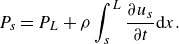 \begin{equation} P_{s}=P_{L}+\rho \int _s^L \displaystyle \frac {\partial u_{s}}{\partial t}{\rm d}x. \end{equation}
For the central region, since the majority of the flow in the TMHV and BHV passes through this region, we can write $Q=A_c u_c$
. Thus,
$Q=A_c u_c$
. Thus, $\partial Q / \partial t= u_c \partial A_c / \partial t + A_c \partial u_c / \partial t$
. At the start of closure, typically
$\partial Q / \partial t= u_c \partial A_c / \partial t + A_c \partial u_c / \partial t$
. At the start of closure, typically $\partial A_c / \partial t$
is low and can be ignored relative to
$\partial A_c / \partial t$
is low and can be ignored relative to $\partial u_c / \partial t$
. Consequently, the last term of (F6) can be ignored and the acceleration term can be written as
$\partial u_c / \partial t$
. Consequently, the last term of (F6) can be ignored and the acceleration term can be written as $ \partial u_c / \partial t = (1/A_c)(\partial Q / \partial t)$
. The central pressure for the TMHV and the BHV could therefore be written as
$ \partial u_c / \partial t = (1/A_c)(\partial Q / \partial t)$
. The central pressure for the TMHV and the BHV could therefore be written as
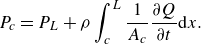 \begin{equation} P_{c}=P_{L}+\rho \int _c^L \displaystyle \frac {1}{A_c} \frac {\partial Q}{\partial t}{\rm d}x. \end{equation}
Since both, $\partial u_s / \partial t \lt 0$
and
$\partial u_s / \partial t \lt 0$
and $\partial Q / \partial t \lt 0$
during the cardiac deceleration and the flow decelerate at a higher rate in the central jet compared with the sinuses as found by our results,
$\partial Q / \partial t \lt 0$
during the cardiac deceleration and the flow decelerate at a higher rate in the central jet compared with the sinuses as found by our results, $|\partial u_s / \partial t| \lt | \partial Q / \partial t |$
, and the above equations could be compared to yield
$|\partial u_s / \partial t| \lt | \partial Q / \partial t |$
, and the above equations could be compared to yield
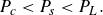 \begin{equation} P_c\lt P_s\lt P_L .\end{equation}
Note that the compliance of the aorta did not affect the above conclusion as long as the assumption $u_s \ll 1$
remains valid.
$u_s \ll 1$
remains valid.
For the BMHV, where the area-weighted averaged side jet velocity ( $u_s$
) is close to the central velocity (
$u_s$
) is close to the central velocity ( $u_c$
) and assuming the flow rate is distributed proportional to the area along with other discussed assumptions about the spatial derivative and the slow start of closure, we have
$u_c$
) and assuming the flow rate is distributed proportional to the area along with other discussed assumptions about the spatial derivative and the slow start of closure, we have $ \partial u_c / \partial t = A_s/(A_t A_c) \partial Q / \partial t$
and
$ \partial u_c / \partial t = A_s/(A_t A_c) \partial Q / \partial t$
and $ \partial u_s / \partial t = A_c/(A_t A_s) \partial Q / \partial t$
, resulting in
$ \partial u_s / \partial t = A_c/(A_t A_s) \partial Q / \partial t$
, resulting in
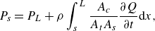 \begin{equation} P_{s}=P_{L}+\rho \int _s^L \displaystyle \frac {A_c}{A_t A_s} \frac {\partial Q}{\partial t}{\rm d}x, \end{equation}
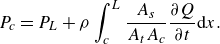 \begin{equation} P_{c}=P_{L}+\rho \int _c^L \displaystyle \frac {A_s}{A_t A_c} \frac {\partial Q}{\partial t}{\rm d}x .\end{equation}
Typically the side and central areas for a BMHV are similar ( $A_s \approx A_c$
) during the deceleration, which results in
$A_s \approx A_c$
) during the deceleration, which results in
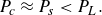 \begin{equation} P_c \approx P_s\lt P_L. \end{equation}
The analysis of the simplified 1-D model mainly suggests that the rigid aorta assumption may not affect the conclusions of this work.


 Open access