


1. Introduction
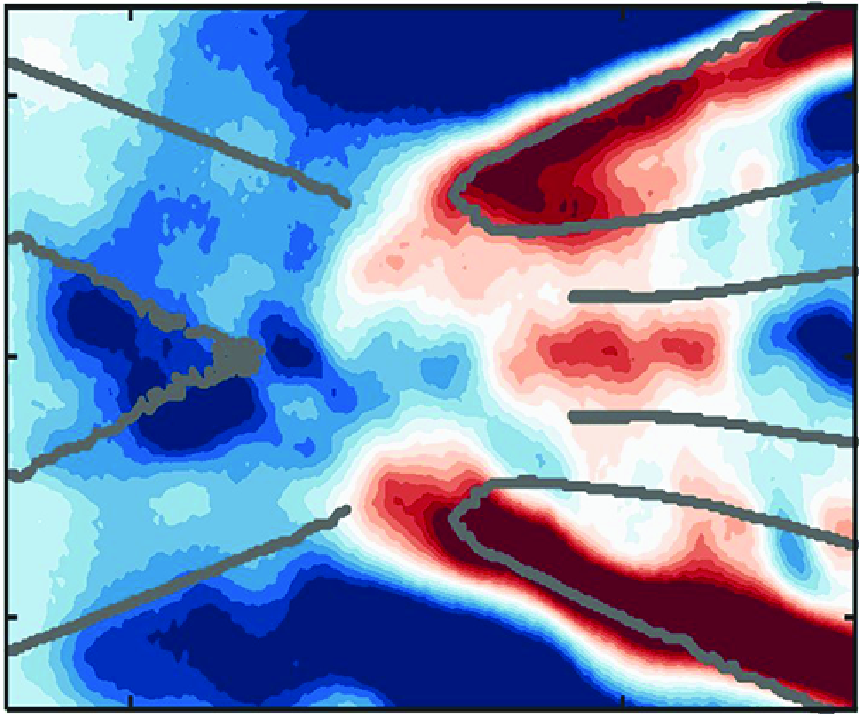
The dynamics of the wake behind a circular cylinder placed in supersonic flow is complex and not well understood. Recently, the authors utilised a high-speed focussing schlieren system to reveal several aspects of the supersonic cylinder wake dynamics (Awasthi et al. Reference Awasthi, McCreton, Moreau and Doolan2022). Figure 1 shows some of the salient wake features revealed in this study through modal analysis of their schlieren dataset. Consistent with some recent studies (Schmidt & Shepherd Reference Schmidt and Shepherd2015; Xu & Ni Reference Xu and Ni2018; Thasu & Duvvuri Reference Thasu and Duvvuri2022), they showed that the frequency of cylinder vortex shedding in supersonic flows was significantly higher than that in the incompressible case. They also showed that the shedding develops downstream of the recompression region in the wake and is not present (or is too weak) in the free shear layers and the recirculation region. Interestingly, they also showed that the periodicity associated with the canonical incompressible case, although weaker, is also present in the early wake, but it dissipates rapidly as the wake develops. The wake instabilities (shown in figure 1) were also found to be symmetric in nature likely due to the streamwise pulsating motion of the reattachment region which has been reported in previous studies on supersonic planar wakes (Scarano & Oudheusden Reference Scarano and Oudheusden2003; Humble, Scarano & van Oudheusden Reference Humble, Scarano and van Oudheusden2007). Through a wavenumber analysis of the proper orthogonal decomposition (POD) modes of bandpass-filtered schlieren images, they found evidence which suggests that the vortex shedding in the supersonic case may be a result of aeroacoustic resonance brought on by an interaction between upstream travelling acoustic waves and downstream propagating disturbances. Lastly, the cylinder wake was also shown to exhibit low-frequency unsteadiness due to oscillations of the recompression shocks similar to that observed in flows over a compression ramp (Poggie & Smits Reference Poggie and Smits2001) and axisymmetric wakes (Simon et al. Reference Simon, Deck, Guillen, Sagaut and Merlen2007). The purpose of this paper is to further describe the behaviour of the coherent oscillations observed in the previous study, establish the mechanism behind the aeroacoustic resonance responsible for vortex shedding and clarify the nature of both the aeroacoustic and hydrodynamic instabilities that exist in the cylinder wake. For a detailed background on supersonic planar wake flows (the category to which the present flow belongs), see Awasthi et al. (Reference Awasthi, McCreton, Moreau and Doolan2022).

Figure 1. Leading POD mode of the focussing schlieren light intensity fluctuations in the wake of a 12 mm circular cylinder bandpass filtered around the shedding frequency ( $St_d$
= 0.42, where
$St_d$
= 0.42, where $St_d$
is the Strouhal number based on the cylinder diameter). Some salient features of the wake have been highlighted. Figure adapted from Awasthi et al. (Reference Awasthi, McCreton, Moreau and Doolan2022).
$St_d$
is the Strouhal number based on the cylinder diameter). Some salient features of the wake have been highlighted. Figure adapted from Awasthi et al. (Reference Awasthi, McCreton, Moreau and Doolan2022).
Modal analysis of high-speed flows can provide useful information about the space–time characteristics of coherent structures provided that the data are spatially and temporally resolved. This task in supersonic flows is often cumbersome if conventional techniques such as a pair of hot-wire probes or a high-speed particle image velocimetry system is utilised. An alternative approach that is relatively simpler, and is becoming popular, is to use a high-speed camera with schlieren imaging to obtain flow information that is well suited for modal analysis methods such as POD, spectral POD (SPOD) and dynamic mode decomposition. The schlieren images provide a light intensity value in each pixel of the image that is proportional to the density gradient in the flow field with the gradient direction determined by the orientation of the knife edge (see Settles (Reference Settles2001) for a detailed description of schlieren imaging). These intensity values can then be decomposed using any of the above mentioned methods to analyse the behaviour of coherent flow structures. Some recent examples of problems that have been studied through modal decomposition techniques applied to high-speed schlieren datasets include high-speed jets (Berry, Magstadt & Glauser Reference Berry, Magstadt and Glauser2017; Price, Gragston & Kreth Reference Price, Gragston and Kreth2020; Padilla-Montero et al. Reference Padilla-Montero, Rodríguez, Jaunet and Jordan2024), shock waves and boundary layers (Cottier & Combs Reference Cottier and Combs2020; Butler & Laurence Reference Butler and Laurence2021), supersonic cavity flow (Desikan et al. Reference Desikan, Pandian, Simha and Sahoo2022), base flow (Lawless, Nicotra & Jewell Reference Lawless, Nicotra and Jewell2024) and even supersonic flow (Mach 4) over a circular cylinder (Thasu & Duvvuri Reference Thasu and Duvvuri2022).
The purpose of the present work is to understand the spatio-temporal behaviour of the wake generated by a circular cylinder placed in a Mach 3 flow through an analysis of the high-speed focussing schlieren images. High-speed schlieren imaging performed using both a horizontal knife edge (flow-parallel orientation) and a vertical knife edge (flow-perpendicular orientation) is utilised in this work to better understand both the convective and acoustic disturbances that exist in the wake. The Reynolds number based on the cylinder diameter and approaching free-stream velocity was $6 \times 10^5$
and focussing schlieren images were acquired at several different framing rates between 100 and 500 kHz to understand the effect of aliasing on the modal decomposition results. The flow conditions and the imaging set-up are the same as Awasthi et al. (Reference Awasthi, McCreton, Moreau and Doolan2022) which the reader can refer to for more details. The organisation of the manuscript is as follows. The focussing schlieren set-up, high-speed imaging parameters and the post-processing of the schlieren images are discussed in § 2. Modal analysis of the schlieren light intensity fluctuations in the cylinder wake using the SPOD is presented in § 3.1. This is followed by a discussion of wavenumber–frequency diagrams extracted from SPOD modes in § 3.2, where it is shown that these diagrams can aid better interpretation of the modes by isolating aliased structures from the true flow structures in SPOD modes. Next, these diagrams and the SPOD modes are utilised to explain the nature of coherent structures in the cylinder wake in § 3.3. The behaviour of the acoustic waves and their interactions in the wake are revealed next in § 3.4. A straightforward aeroacoustic feedback model that can be used to predict the shedding frequency in the wake is also proposed in this section. Finally, a low-order representation of the wake flow field using inversion of the SPOD modes is used to clarify the nature of the bimodal vortex shedding behaviour observed in the wake in § 3.5, before concluding the paper in § 4.
$6 \times 10^5$
and focussing schlieren images were acquired at several different framing rates between 100 and 500 kHz to understand the effect of aliasing on the modal decomposition results. The flow conditions and the imaging set-up are the same as Awasthi et al. (Reference Awasthi, McCreton, Moreau and Doolan2022) which the reader can refer to for more details. The organisation of the manuscript is as follows. The focussing schlieren set-up, high-speed imaging parameters and the post-processing of the schlieren images are discussed in § 2. Modal analysis of the schlieren light intensity fluctuations in the cylinder wake using the SPOD is presented in § 3.1. This is followed by a discussion of wavenumber–frequency diagrams extracted from SPOD modes in § 3.2, where it is shown that these diagrams can aid better interpretation of the modes by isolating aliased structures from the true flow structures in SPOD modes. Next, these diagrams and the SPOD modes are utilised to explain the nature of coherent structures in the cylinder wake in § 3.3. The behaviour of the acoustic waves and their interactions in the wake are revealed next in § 3.4. A straightforward aeroacoustic feedback model that can be used to predict the shedding frequency in the wake is also proposed in this section. Finally, a low-order representation of the wake flow field using inversion of the SPOD modes is used to clarify the nature of the bimodal vortex shedding behaviour observed in the wake in § 3.5, before concluding the paper in § 4.
2. Experimental set-up
2.1. The UNSW Mach 3 supersonic wind tunnel and wake generator
The measurements were performed in the Mach 3 Supersonic Wind Tunnel at the University of New South Wales. The facility is a blow-down to atmosphere wind tunnel with a 142.6 mm $\times$
101.6 mm cross-section that can provide a Mach 3 (
$\times$
101.6 mm cross-section that can provide a Mach 3 ( $\pm$
0.013) flow up to approximately 16 s. A full-span, 12 mm diameter circular cylinder was installed 292 mm downstream of the wind tunnel nozzle throat at the mid-height of the test section. Two 119 mm diameter optical windows were installed downstream of the cylinder to enable schlieren imaging. The Reynolds number based on cylinder diameter and free-stream velocity in the measurements was
$\pm$
0.013) flow up to approximately 16 s. A full-span, 12 mm diameter circular cylinder was installed 292 mm downstream of the wind tunnel nozzle throat at the mid-height of the test section. Two 119 mm diameter optical windows were installed downstream of the cylinder to enable schlieren imaging. The Reynolds number based on cylinder diameter and free-stream velocity in the measurements was $6.0 \times 10^5$
. Further details of this facility and the circular cylinder set-up can be found in Awasthi et al. (Reference Awasthi, McCreton, Moreau and Doolan2022). The coordinate system we will follow in this work is centred at the cylinder centre with
$6.0 \times 10^5$
. Further details of this facility and the circular cylinder set-up can be found in Awasthi et al. (Reference Awasthi, McCreton, Moreau and Doolan2022). The coordinate system we will follow in this work is centred at the cylinder centre with $x$
and
$x$
and $y$
as the streamwise and transverse coordinates, respectively.
$y$
as the streamwise and transverse coordinates, respectively.
2.2. Focussing schlieren system and post-processing of schlieren images
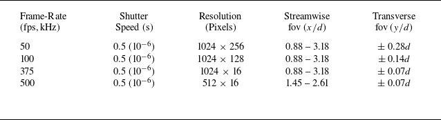
The optical set-up and characteristics of the focussing schlieren system used to visualise the cylinder wake can be found in Awasthi et al. (Reference Awasthi, McCreton, Moreau and Doolan2022). The system has been shown to effectively suppress the schlieren light deflections due to the density gradients within the sidewall boundary layers, thereby minimising the effects of the three-dimensional flow near the cylinder/wall junction on the images. The schlieren imaging was performed with the knife edge positioned both parallel (horizontal orientation) and perpendicular (vertical orientation) to the free-stream flow direction. The light intensity values yielded by the flow-parallel and flow-perpendicular knife-edge configurations are proportional to the transverse and streamwise gradient of the density, respectively. It has been shown in Awasthi et al. (Reference Awasthi, McCreton, Moreau and Doolan2022) that, for the present flow configuration, a flow-parallel orientation of the knife edge is more suited to the visualisation of turbulent structures, whereas a flow-perpendicular knife-edge orientation is more sensitive to wave-like features in the flow. The schlieren images were recorded using a Photron NOVA S12 monochromatic camera at several different frame rates between 50 and 500 kHz to determine the effect of aliasing on the modal decomposition. Table 1 shows the details of the schlieren imaging for four different frame rates that will be considered in the present study. The table also shows the field-of-view (fov) in the streamwise ( $x$
) and transverse (
$x$
) and transverse ( $y$
) directions for each case (note that the origin of the coordinate system is at the cylinder centre). Note that, due to the data throughput limitation, the size of the fov decreases as the frame rate increases. For sampling rates up to 375 kHz, the fov shrinks only in the transverse direction, but for the 500 kHz dataset, it is affected in both directions.
$y$
) directions for each case (note that the origin of the coordinate system is at the cylinder centre). Note that, due to the data throughput limitation, the size of the fov decreases as the frame rate increases. For sampling rates up to 375 kHz, the fov shrinks only in the transverse direction, but for the 500 kHz dataset, it is affected in both directions.
Table 1. Focussing schlieren imaging parameters.
The schlieren images contain grey scale light intensity values in each pixel that are proportional to the density gradient in the flow field. Thus, each pixel in the schlieren images can be treated as an optical sensor and the resulting spatially and temporally resolved data matrix of grey scale intensities can be analysed further through several spatio-temporal processing methods. Here, we choose the SPOD algorithm (Schmidt et al. Reference Schmidt, Towne, Rigas, Colonius and Brès2018; Towne, Schmidt & Colonius Reference Towne, Schmidt and Colonius2018; Schmidt & Colonius Reference Schmidt and Colonius2020) to decompose the schlieren light intensity fluctuations into orthogonal spatial modes at each frequency, which effectively reveals wake oscillations that are coherent in both space and time. The SPOD was calculated using the algorithm developed by Towne et al. (Reference Towne, Schmidt and Colonius2018). The cross-spectral matrix required for SPOD was calculated using Welch’s periodogram with a varying record length (to yield the same 390.6 Hz resolution at different sampling rates), a Hanning window and an overlap of 50 % between adjacent records. In the present work, we also use SPOD to perform a low-order reconstruction of the flow field to better understand the nature of wake instabilities. The reconstruction, discussed further in § 3.5, was carried out using the frequency-domain approach described in Nekkanti & Schmidt (Reference Nekkanti and Schmidt2021). Several reconstructed schlieren movies that reveal salient aspects of the wake flow field have been included with this paper as supplementary material.
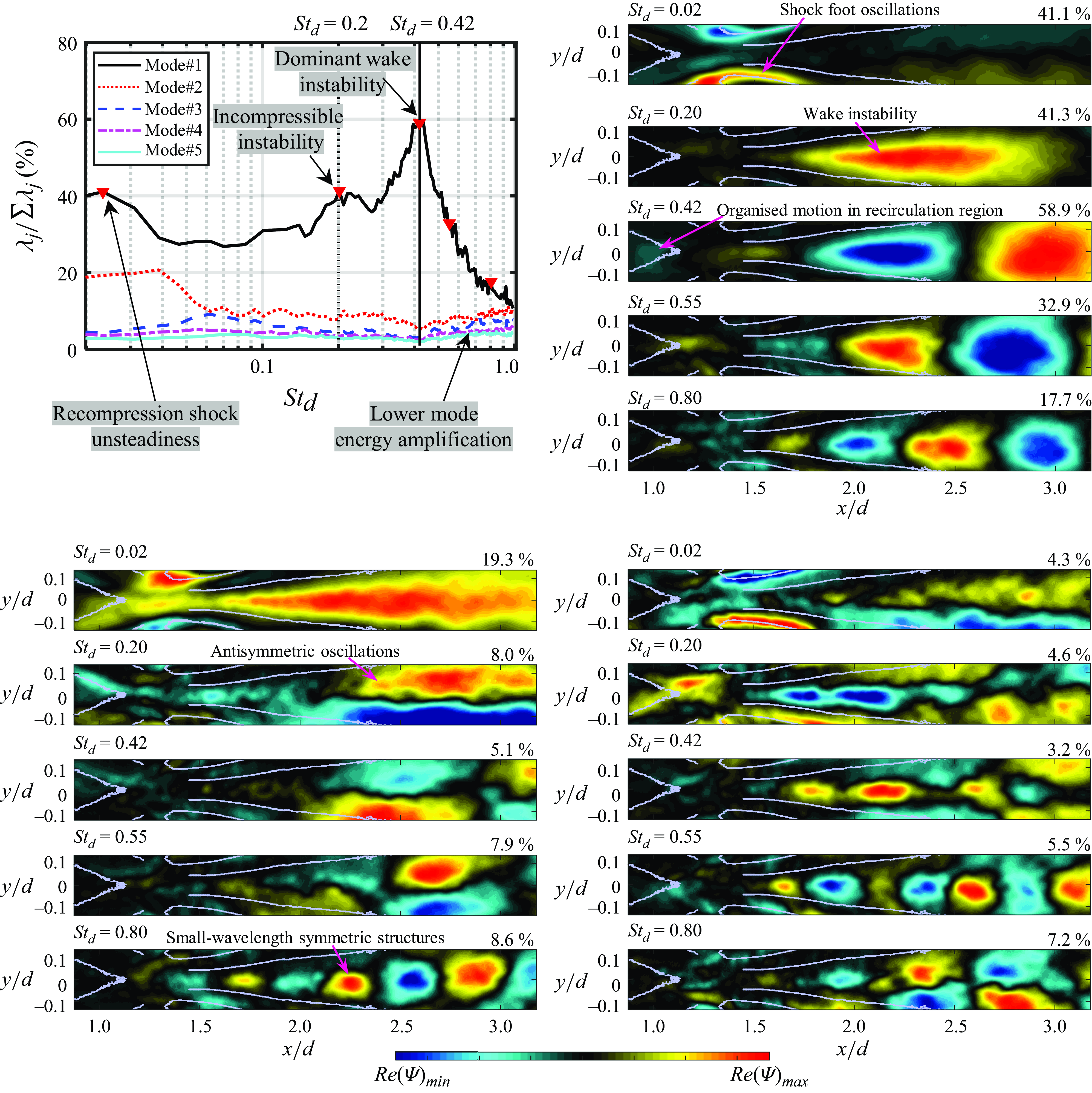
Figure 2. Spectral proper orthogonal decomposition of focussing schlieren light intensity fluctuations in the wake of the 12 mm cylinder. The SPOD eigenspectra for the leading five modes is shown in (a) along with markers ( $\blacktriangledown$
) corresponding to the frequencies for which the first, second and third SPOD modes (real part) are shown in (b), (c) and (d), respectively. In (b), (c) and (d),the frequencies and the fractional energy contribution of each mode are shown at the top-left and top-right of each, respectively. The colour scale (shown at the bottom) for each mode stretches between the minimum and maximum SPOD eigenvector magnitude (modal amplitude) within each mode, with 51 colour levels shown such that shades of blue represent negative values, black represents a value of zero and shades of yellow and red represent positive values. Subsequent presentation of SPOD modes in this paper follows the same colour scheme.
$\blacktriangledown$
) corresponding to the frequencies for which the first, second and third SPOD modes (real part) are shown in (b), (c) and (d), respectively. In (b), (c) and (d),the frequencies and the fractional energy contribution of each mode are shown at the top-left and top-right of each, respectively. The colour scale (shown at the bottom) for each mode stretches between the minimum and maximum SPOD eigenvector magnitude (modal amplitude) within each mode, with 51 colour levels shown such that shades of blue represent negative values, black represents a value of zero and shades of yellow and red represent positive values. Subsequent presentation of SPOD modes in this paper follows the same colour scheme.
3. Results and discussion
3.1. Modal description of the cylinder wake
Figure 2(a) shows the SPOD eigenvalue ( $\lambda$
) spectra for the five leading modes in the cylinder wake from the 100 kHz flow-parallel knife-edge dataset. At each frequency, the eigenvalue for each mode has been normalised on the sum of eigenvalues across all the modes such that they represent the fractional contribution of each mode (as a percentage) to the overall energy in the dataset. The first mode remains dominant through a broad frequency range and shows a prominent peak around
$\lambda$
) spectra for the five leading modes in the cylinder wake from the 100 kHz flow-parallel knife-edge dataset. At each frequency, the eigenvalue for each mode has been normalised on the sum of eigenvalues across all the modes such that they represent the fractional contribution of each mode (as a percentage) to the overall energy in the dataset. The first mode remains dominant through a broad frequency range and shows a prominent peak around $St_d$
= 0.42 which, as noted by Awasthi et al. (Reference Awasthi, McCreton, Moreau and Doolan2022), is the dominant wake instability. A smaller, less prominent maximum in the spectra can also be observed around
$St_d$
= 0.42 which, as noted by Awasthi et al. (Reference Awasthi, McCreton, Moreau and Doolan2022), is the dominant wake instability. A smaller, less prominent maximum in the spectra can also be observed around $St_d$
= 0.2, which is the canonical Kelvin–Helmholtz-type instability of the incompressible case. Later, we show that these two instabilities are fundamentally different and unrelated to each other. The bimodal shedding behaviour of the cylinder wake was previously also discussed in Awasthi et al. (Reference Awasthi, McCreton, Moreau and Doolan2022) through Fourier analysis of the schlieren light intensity fluctuations. Coming back to figure 2(a), we note that the lower-order modes contribute less than 10 % to the overall energy in the dataset, with the exception of the contribution from the second mode at low frequencies (
$St_d$
= 0.2, which is the canonical Kelvin–Helmholtz-type instability of the incompressible case. Later, we show that these two instabilities are fundamentally different and unrelated to each other. The bimodal shedding behaviour of the cylinder wake was previously also discussed in Awasthi et al. (Reference Awasthi, McCreton, Moreau and Doolan2022) through Fourier analysis of the schlieren light intensity fluctuations. Coming back to figure 2(a), we note that the lower-order modes contribute less than 10 % to the overall energy in the dataset, with the exception of the contribution from the second mode at low frequencies ( $St_d\lt$
0.04) which is approximately 20 %. As shown momentarily, this is because the energy in the leading mode at these frequencies is dominated by the low-frequency oscillation of recompression shocks which results in the convective wake instability appearing in the second mode, thereby increasing its contribution. Interestingly, each of the lower-order modes also shows a slight increase in energy levels at frequencies greater than
$St_d\lt$
0.04) which is approximately 20 %. As shown momentarily, this is because the energy in the leading mode at these frequencies is dominated by the low-frequency oscillation of recompression shocks which results in the convective wake instability appearing in the second mode, thereby increasing its contribution. Interestingly, each of the lower-order modes also shows a slight increase in energy levels at frequencies greater than $St_d$
= 0.42, with the second mode showing levels comparable to that of the first mode towards the highest frequencies. It is shown in § 3.3 that this energy increase of lower-order modes towards the higher frequencies may be attributed to aliasing in the schlieren datasets.
$St_d$
= 0.42, with the second mode showing levels comparable to that of the first mode towards the highest frequencies. It is shown in § 3.3 that this energy increase of lower-order modes towards the higher frequencies may be attributed to aliasing in the schlieren datasets.
Now consider the mode shapes (real part of the SPOD eigenvector) for the three leading SPOD modes at five different frequencies, as shown in figure 2(b–d). The frequency of each mode and its fractional contribution to the overall energy in the dataset are listed to the top-left and top-right, respectively. To aid better interpretation of these modes, the edges of salient flow features in the flow field determined using a custom edge-detection algorithm described in Awasthi et al. (Reference Awasthi, McCreton, Moreau and Doolan2022) have been superimposed upon each mode for spatial reference (see figure 1 above for the features represented by these edges). The mode shape is a function of frequency and four different features in these modes can be identified: low-frequency shock oscillations, symmetric (varicose) and anti-symmetric (sinuous) wake instabilities and a small-wavelength symmetric instability. The leading mode (figure 2
b) is dominated by the coherent structures in the wake for each frequency, except the lowest frequency ( $St_d$
= 0.02) where the oscillation of the recompression shock feet is the most prominent feature. The convective wake instability at this low frequency appears in the second mode instead (top row, figure 2
c) and it is accompanied by shock feet oscillations, suggesting that the interaction between the oncoming free shear layer and the recompression shock is an important feature of the cylinder wake dynamics at low frequencies. The coherent structures in the wake have the same appearance as the bandpass-filtered POD modes of Awasthi et al. (Reference Awasthi, McCreton, Moreau and Doolan2022), and as explained there, their symmetric nature implies a varicose-type instability, as opposed to a flapping-type motion commonly observed in low Mach number wakes. This behaviour is consistent with past measurements of a Mach 2 planar wake (Scarano & Oudheusden Reference Scarano and Oudheusden2003) where the streamwise pulsation of the unsteady reattachment region was found to be the origin of this varicose-type instability. The leading mode at the shedding frequency (
$St_d$
= 0.02) where the oscillation of the recompression shock feet is the most prominent feature. The convective wake instability at this low frequency appears in the second mode instead (top row, figure 2
c) and it is accompanied by shock feet oscillations, suggesting that the interaction between the oncoming free shear layer and the recompression shock is an important feature of the cylinder wake dynamics at low frequencies. The coherent structures in the wake have the same appearance as the bandpass-filtered POD modes of Awasthi et al. (Reference Awasthi, McCreton, Moreau and Doolan2022), and as explained there, their symmetric nature implies a varicose-type instability, as opposed to a flapping-type motion commonly observed in low Mach number wakes. This behaviour is consistent with past measurements of a Mach 2 planar wake (Scarano & Oudheusden Reference Scarano and Oudheusden2003) where the streamwise pulsation of the unsteady reattachment region was found to be the origin of this varicose-type instability. The leading mode at the shedding frequency ( $St_d$
= 0.42, third row in figure 2
b) is similar to that at other frequencies, except that a faint, but organised, disturbance can be observed within the recirculation region around
$St_d$
= 0.42, third row in figure 2
b) is similar to that at other frequencies, except that a faint, but organised, disturbance can be observed within the recirculation region around $x/d$
= 1.0, suggesting that the shedding may have its origin within the recirculation region behind the cylinder (we later show that this is indeed the case). Note that the presence of the convective wake instability in the second SPOD mode at
$x/d$
= 1.0, suggesting that the shedding may have its origin within the recirculation region behind the cylinder (we later show that this is indeed the case). Note that the presence of the convective wake instability in the second SPOD mode at $St_d$
= 0.02, instead of the first mode, is the reason for the low-frequency peak in the eigenspectrum for this mode.
$St_d$
= 0.02, instead of the first mode, is the reason for the low-frequency peak in the eigenspectrum for this mode.
Besides the shock oscillations and the symmetric wake instabilities, the third notable feature of the wake that is revealed in the second SPOD mode for $St_d$
= 0.2, 0.42 and 0.55 (figure 2
c) is an anti-symmetric oscillation, which suggests that a flapping-type motion, although weaker than the varicose mode, may also exist in the wake. A low-order reconstruction of the temporal evolution of the flow field based on the SPOD modes, which is discussed later in § 3.5, was used to confirm that the symmetric and anti-symmetric SPOD modes here indeed correspond to a streamwise pulsating and flapping-type motions, respectively (see Movie 1 and Movie 2 in the supplementary material). Note that, for
$St_d$
= 0.2, 0.42 and 0.55 (figure 2
c) is an anti-symmetric oscillation, which suggests that a flapping-type motion, although weaker than the varicose mode, may also exist in the wake. A low-order reconstruction of the temporal evolution of the flow field based on the SPOD modes, which is discussed later in § 3.5, was used to confirm that the symmetric and anti-symmetric SPOD modes here indeed correspond to a streamwise pulsating and flapping-type motions, respectively (see Movie 1 and Movie 2 in the supplementary material). Note that, for $St_d$
= 0.02 and 0.80, the flapping motion appears in the third mode (figure 2
d), where for
$St_d$
= 0.02 and 0.80, the flapping motion appears in the third mode (figure 2
d), where for $St_d$
= 0.02 it is accompanied by strong shock feet oscillation of opposite sign. This mode switching for
$St_d$
= 0.02 it is accompanied by strong shock feet oscillation of opposite sign. This mode switching for $St_d$
= 0.02 occurs because the leading mode is dominated by the low-frequency shock oscillations, which shifts the two types of wake instabilities down a mode number. On the other hand, at
$St_d$
= 0.02 occurs because the leading mode is dominated by the low-frequency shock oscillations, which shifts the two types of wake instabilities down a mode number. On the other hand, at $St_d$
= 0.80 it is the appearance of symmetric wake instabilities in the second mode (bottom row, figure 2
c) that is responsible for mode switching. These symmetric structures have a similar appearance to the leading mode instability at this frequency, but the size and wavelength of the structures are smaller. It will be shown momentarily that these structures are an aliased version of the convective instability itself, rather than a feature of the flow.
$St_d$
= 0.80 it is the appearance of symmetric wake instabilities in the second mode (bottom row, figure 2
c) that is responsible for mode switching. These symmetric structures have a similar appearance to the leading mode instability at this frequency, but the size and wavelength of the structures are smaller. It will be shown momentarily that these structures are an aliased version of the convective instability itself, rather than a feature of the flow.
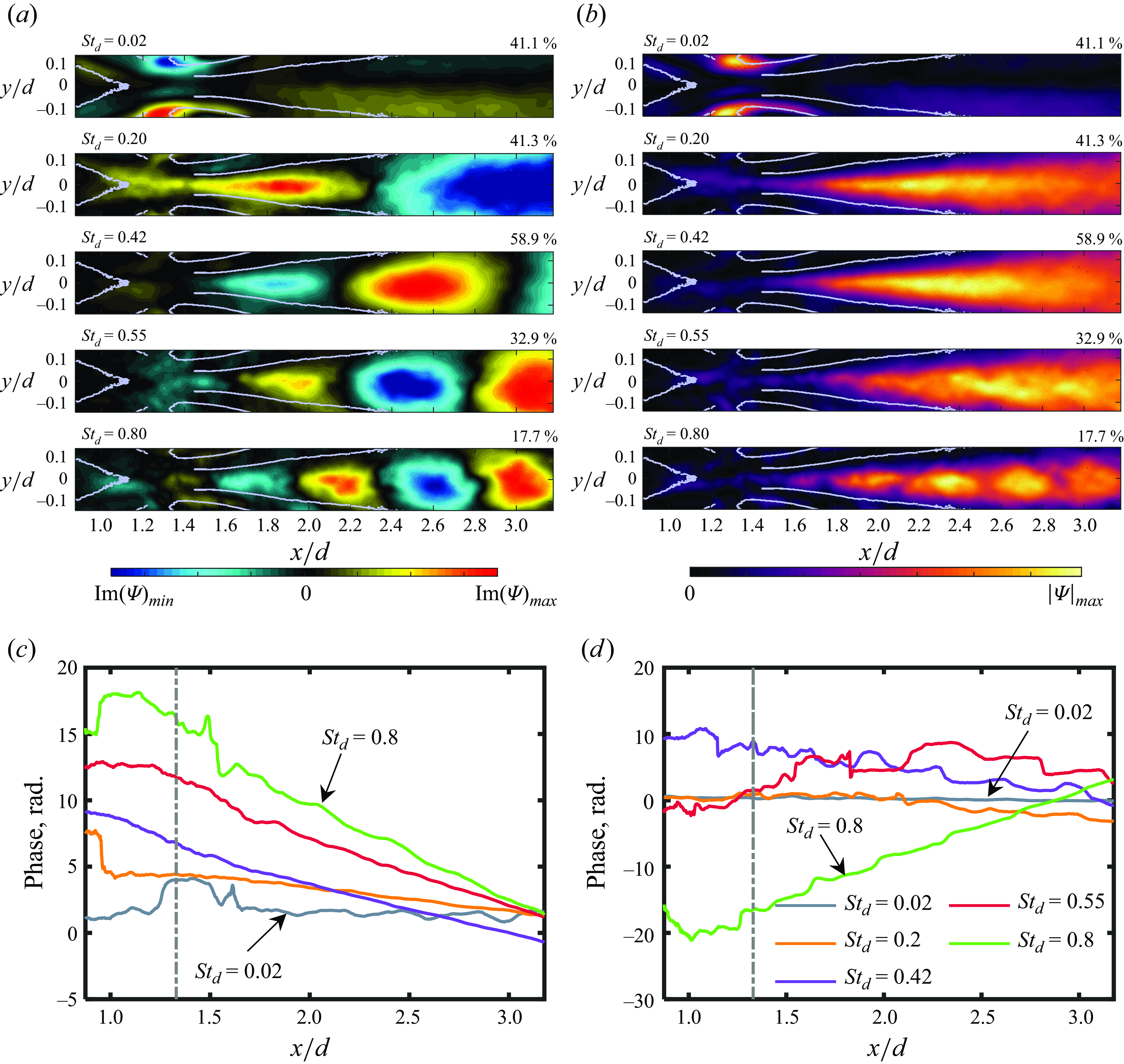
Figure 3. The SPOD eigenvector analysis at five different frequencies considered in figure 2. The imaginary part of the SPOD eigenvector and the amplitude for the most energetic mode are shown in (a) and (b), respectively. The format of these plots is the same as figure 2. The phase of the SPOD eigenvector along the wake centreline for the five frequencies is shown in (c) and (d) for the first and the second SPOD mode, respectively. The legend for (c) and (d) is shown in (d), and the vertical broken line in each plot represents the mean reattachment location in the streamwise direction extracted from Awasthi et al. (Reference Awasthi, McCreton, Moreau and Doolan2022).
Figure 3(a) shows the imaginary part of the leading SPOD mode at the five frequencies for which the real part was shown in figure 2(b). The imaginary part shows the same flow structures as the real part, just shifted in space. Although not shown, this is also true for lower-order SPOD modes and in the next section we will utilise this property of SPOD to generate bi-directional modal wavenumber–frequency spectra which are useful for interpreting the SPOD mode shapes. Figure 3(b) shows the amplitude of the leading SPOD eigenvectors (the absolute value) for the same five frequencies as in (a). Because the amplitude of the SPOD mode is a combination of both the real and imaginary parts which are phase shifted, these images essentially show a large fraction of the total variance in the dataset at each frequency. As expected, besides the mode at the lowest frequency, which is dominated by the oscillations of the shock foot, the remaining modes show that the leading mode is dominated by the wake instabilities.
Since the SPOD eigenvectors are complex, they can also be utilised to extract the phase spectrum associated with a SPOD mode. Figure 3(c) shows the phase of the most energetic SPOD eigenvector along the wake centreline ( $y$
= 0) as a function of the streamwise distance at the same five frequencies for which the SPOD mode shapes have been previously discussed. The vertical broken line in the plot represents the mean reattachment location taken from Awasthi et al. (Reference Awasthi, McCreton, Moreau and Doolan2022). Besides
$y$
= 0) as a function of the streamwise distance at the same five frequencies for which the SPOD mode shapes have been previously discussed. The vertical broken line in the plot represents the mean reattachment location taken from Awasthi et al. (Reference Awasthi, McCreton, Moreau and Doolan2022). Besides $St_d$
= 0.02, the phase beyond the reattachment point generally shows a linear relationship with distance which is typical of convective shear flows. There is some nonlinearity closer to the reattachment location, but that is to be expected since coherency in this region is weaker than in the wake. At the lowest frequency, the phase is nonlinear since, as shown by the SPOD mode shapes earlier, the leading mode at this frequency is dominated by the shock foot oscillations and the wake instabilities appear in the second mode (figure 2
c). The linear phase relationship with distance can be exploited to extract phase convection velocities at each frequency. The phase convection velocity can be calculated as
$St_d$
= 0.02, the phase beyond the reattachment point generally shows a linear relationship with distance which is typical of convective shear flows. There is some nonlinearity closer to the reattachment location, but that is to be expected since coherency in this region is weaker than in the wake. At the lowest frequency, the phase is nonlinear since, as shown by the SPOD mode shapes earlier, the leading mode at this frequency is dominated by the shock foot oscillations and the wake instabilities appear in the second mode (figure 2
c). The linear phase relationship with distance can be exploited to extract phase convection velocities at each frequency. The phase convection velocity can be calculated as
 \begin{equation} {U_{c_p} = \frac {2\pi f}{{\rm d}\phi /{\rm d}x}}, \end{equation}
where $U_{c_p}$
is the phase convection velocity in (in
$U_{c_p}$
is the phase convection velocity in (in $\rm m\, s^{-1}$
),
$\rm m\, s^{-1}$
), $f$
is the frequency (in
$f$
is the frequency (in $Hz$
) and
$Hz$
) and ${\rm d}\phi /{\rm d}x$
is the slope of the phase curve. For each frequency, the phase convection velocity was found to be approximately 70 % of the free-stream velocity
${\rm d}\phi /{\rm d}x$
is the slope of the phase curve. For each frequency, the phase convection velocity was found to be approximately 70 % of the free-stream velocity $(U_\infty)$
which, as shown in the next section, is consistent with the phase velocities extracted from the modal wavenumber–frequency spectra. The phase of the second most energetic eigenvector at the same five frequencies is shown in figure 3(d). Here, the phase for
$(U_\infty)$
which, as shown in the next section, is consistent with the phase velocities extracted from the modal wavenumber–frequency spectra. The phase of the second most energetic eigenvector at the same five frequencies is shown in figure 3(d). Here, the phase for $St_d$
= 0.02 shows a linear relationship with distance (although this is difficult to see because of its shallow slope) since at this frequency the convective wake instabilities appear in the second mode. The phase curves at
$St_d$
= 0.02 shows a linear relationship with distance (although this is difficult to see because of its shallow slope) since at this frequency the convective wake instabilities appear in the second mode. The phase curves at $St_d$
= 0.2, 0.42 and 0.55 have a similar appearance and show a nonlinear behaviour. This is likely because, as shown in figure 2 (as well as in the supplemental material), the second mode at these frequencies is not associated with the symmetric wake instabilities that are squeezed out of the reattachment region and convect downstream, but rather with the flapping-type motion of the shear layer. Finally, it is interesting to note that the phase for
$St_d$
= 0.2, 0.42 and 0.55 have a similar appearance and show a nonlinear behaviour. This is likely because, as shown in figure 2 (as well as in the supplemental material), the second mode at these frequencies is not associated with the symmetric wake instabilities that are squeezed out of the reattachment region and convect downstream, but rather with the flapping-type motion of the shear layer. Finally, it is interesting to note that the phase for $St_d$
= 0.8 is similar to that in the leading mode, but its slope has an opposite sign (positive slope) which indicates a negative phase convection velocity. This is because, as pointed out earlier and shown in the next section, the second SPOD mode at this frequency contains an aliased version of the convective instabilities with negative phase velocities.
$St_d$
= 0.8 is similar to that in the leading mode, but its slope has an opposite sign (positive slope) which indicates a negative phase convection velocity. This is because, as pointed out earlier and shown in the next section, the second SPOD mode at this frequency contains an aliased version of the convective instabilities with negative phase velocities.
3.2. Wavenumber–frequency diagrams of SPOD eigenvectors
Although the SPOD modes and eigenspectra themselves are useful in developing an understanding of the spatio-temporal periodicities hidden in the schlieren images, here, we show that a wavenumber decomposition of these modes can aid a clearer and more informed interpretation of the SPOD results. The SPOD eigenvectors at each frequency can be Fourier transformed in the streamwise direction to obtain a streamwise wavenumber–frequency spectrum (referred to as $\kappa _x-f$
spectrum from hereon) associated with each mode. Since SPOD eigenvectors for each mode are complex with real and imaginary parts representing the same flow feature with a spatial phase shift, Fourier transforming them in space yields a bi-directional spectrum with both positive and negative wavenumber information. This information may be utilised to identify downstream and upstream propagating waves since they will appear as disturbances with positive and negative wavenumbers, respectively. Note that this approach is similar to that employed in Awasthi et al. (Reference Awasthi, McCreton, Moreau and Doolan2022), except there POD modes of temporally bandpass-filtered schlieren images that were in quadrature were used to form a complex eigenvector. The advantage of the current approach is that a full
$\kappa _x-f$
spectrum from hereon) associated with each mode. Since SPOD eigenvectors for each mode are complex with real and imaginary parts representing the same flow feature with a spatial phase shift, Fourier transforming them in space yields a bi-directional spectrum with both positive and negative wavenumber information. This information may be utilised to identify downstream and upstream propagating waves since they will appear as disturbances with positive and negative wavenumbers, respectively. Note that this approach is similar to that employed in Awasthi et al. (Reference Awasthi, McCreton, Moreau and Doolan2022), except there POD modes of temporally bandpass-filtered schlieren images that were in quadrature were used to form a complex eigenvector. The advantage of the current approach is that a full $\kappa _x-f$
spectrum associated with each mode can be obtained without resorting to bandpass filtering the data across several frequency bands and then searching for modes that are in quadrature.
$\kappa _x-f$
spectrum associated with each mode can be obtained without resorting to bandpass filtering the data across several frequency bands and then searching for modes that are in quadrature.
The $\kappa _x-f$
spectra were obtained by calculating the spatial Fourier transform of the SPOD eigenvector along the wake centreline for each mode. To assess the effect of aliasing on the SPOD eigenvectors, the calculation was carried out for the schlieren datasets with the three highest sampling rates (see table 1). For consistency, the SPOD for each dataset was performed on a truncated image with resolution and fov matching that of the highest sampling rate dataset (500 kHz; see table 1). The SPOD eigenvector at each frequency was zero padded before Fourier transforming to yield a wavenumber resolution of
$\kappa _x-f$
spectra were obtained by calculating the spatial Fourier transform of the SPOD eigenvector along the wake centreline for each mode. To assess the effect of aliasing on the SPOD eigenvectors, the calculation was carried out for the schlieren datasets with the three highest sampling rates (see table 1). For consistency, the SPOD for each dataset was performed on a truncated image with resolution and fov matching that of the highest sampling rate dataset (500 kHz; see table 1). The SPOD eigenvector at each frequency was zero padded before Fourier transforming to yield a wavenumber resolution of $\kappa _xd$
= 2.7 (where
$\kappa _xd$
= 2.7 (where $\kappa _x$
is in rad m–1). First consider figure 4(a), (b) and (c) which show the
$\kappa _x$
is in rad m–1). First consider figure 4(a), (b) and (c) which show the $\kappa _x-f$
spectrum associated with the first, second and third SPOD eigenvector, respectively, along the wake centreline (
$\kappa _x-f$
spectrum associated with the first, second and third SPOD eigenvector, respectively, along the wake centreline ( $y$
= 0) for the 100 kHz dataset. These plots show the absolute value of the Fourier transform (
$y$
= 0) for the 100 kHz dataset. These plots show the absolute value of the Fourier transform ( $W(\kappa _x,f)$
) normalised on its maximum value on a logarithmic scale with the colour scale (shown at the bottom) limited to two orders of magnitude. The main feature of the spectra for the leading mode is a convective band passing through the origin which has a constant slope of approximately 0.72
$W(\kappa _x,f)$
) normalised on its maximum value on a logarithmic scale with the colour scale (shown at the bottom) limited to two orders of magnitude. The main feature of the spectra for the leading mode is a convective band passing through the origin which has a constant slope of approximately 0.72 $U_\infty$
, implying that the average convective speed of the wake instabilities (
$U_\infty$
, implying that the average convective speed of the wake instabilities ( $U_c$
) is approximately 72 % of the free-stream velocity upstream of the cylinder. This convection velocity value is consistent with what was obtained using the SPOD phase plots in the previous section (figures 3
c and 3
d). For lower modes, this convective band is still present, but its strength and appearance are functions of the mode number and sampling rate which, as explained below, is due to a change in the nature of coherent oscillations being represented by these modes and the presence of aliasing in the schlieren datasets.
$U_c$
) is approximately 72 % of the free-stream velocity upstream of the cylinder. This convection velocity value is consistent with what was obtained using the SPOD phase plots in the previous section (figures 3
c and 3
d). For lower modes, this convective band is still present, but its strength and appearance are functions of the mode number and sampling rate which, as explained below, is due to a change in the nature of coherent oscillations being represented by these modes and the presence of aliasing in the schlieren datasets.
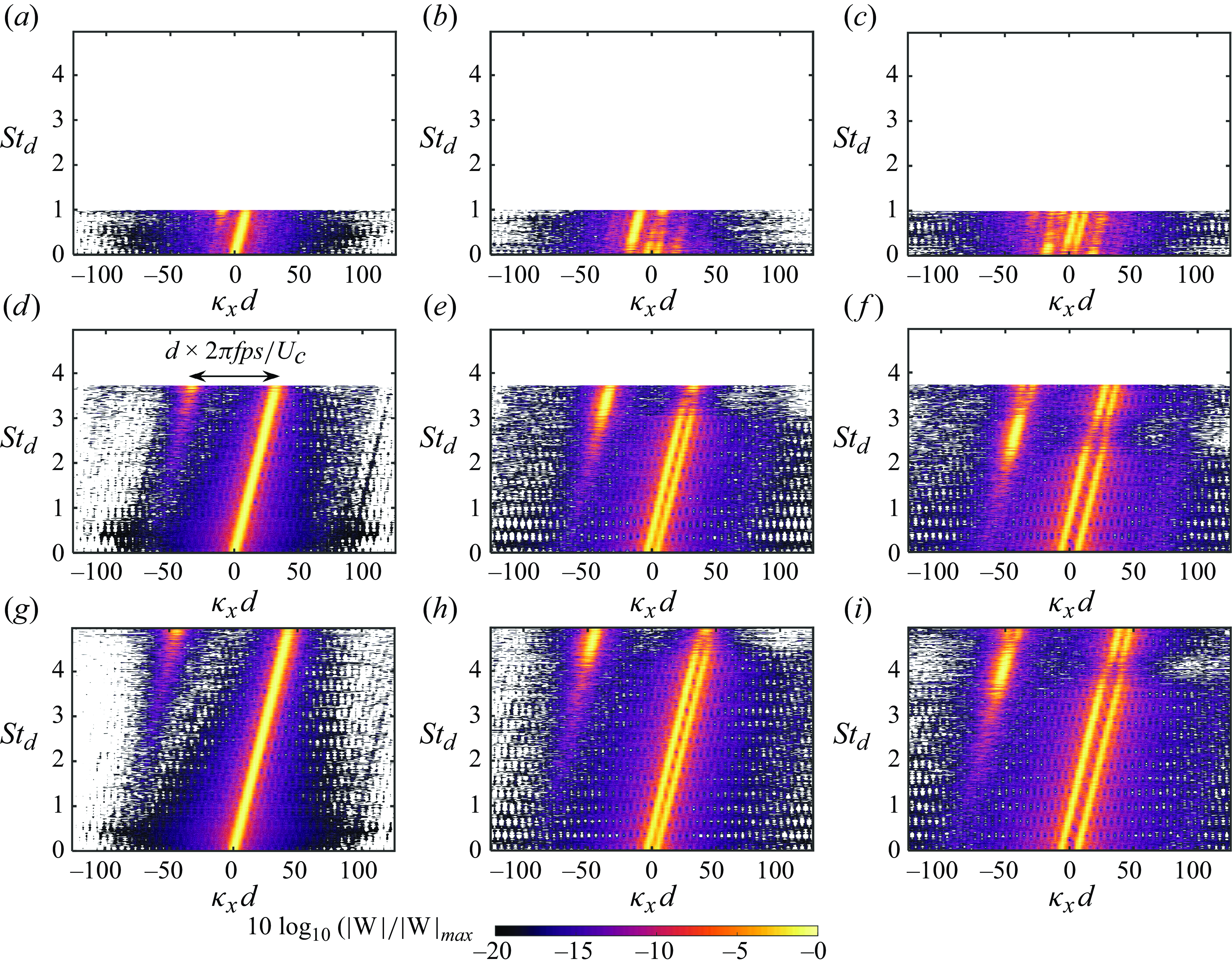
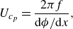
Figure 4. Bi-directional modal wavenumber–frequency spectra for the three leading modes obtained by Fourier transforming the complex SPOD eigenvector along the wake centreline. The spectra are shown for three different sampling rates of 100 kHz (a, b, c); 375 kHz (d, e, f); 500 kHz (g, h, i). The first, second and third columns show the spectra for the first, second and third SPOD modes, respectively.
Besides the convective band passing through the origin, a notable feature of each spectra for the 100 kHz dataset in figure 4(a–c) is the presence of several parallel streaks with the same slope as the convective band. In the first mode, this streak is limited to the highest frequencies for negative wavenumbers, but for lower modes they are present in both the left and right halves of the spectra, and depending on the mode number, at lowest frequencies as well. These streaks are the first sign that the schlieren dataset at 100 kHz contains aliased energy. The aliasing is particularly prominent in the spectra for the second mode (figure 4
b), where its energy exceeds that of the main lobe throughout the frequency range. Along the wavenumber axis, the separation between the main lobe and the side lobes due to aliasing is approximately $\kappa _xd$
= 18, which corresponds to a wavelength of 0.35
$\kappa _xd$
= 18, which corresponds to a wavelength of 0.35 $d$
– the same wavelength reported in Awasthi et al. (Reference Awasthi, McCreton, Moreau and Doolan2022) as the characteristic length scale of a standing wave-type pattern that was revealed through spatial distribution of the frequency-domain coherence function (see figures 11 and 12 in Awasthi et al. (Reference Awasthi, McCreton, Moreau and Doolan2022)). In their results, Awasthi et al. (Reference Awasthi, McCreton, Moreau and Doolan2022) also showed that the standing wave pattern in the wake could be reproduced by isolating the negative and positive wavenumber peaks in the wavenumber transform of POD modes in quadrature. The results here show that the negative wavenumber component, which was previously believed to be an upstream propagating acoustic wave in the wake, is actually a side lobe of the convective instability itself that appears as a wave with negative phase velocity. The negative phase velocity associated with the aliased energy and its prominence in the second SPOD mode is also consistent with the discussion on the SPOD phase in the previous section where it was shown that at
$d$
– the same wavelength reported in Awasthi et al. (Reference Awasthi, McCreton, Moreau and Doolan2022) as the characteristic length scale of a standing wave-type pattern that was revealed through spatial distribution of the frequency-domain coherence function (see figures 11 and 12 in Awasthi et al. (Reference Awasthi, McCreton, Moreau and Doolan2022)). In their results, Awasthi et al. (Reference Awasthi, McCreton, Moreau and Doolan2022) also showed that the standing wave pattern in the wake could be reproduced by isolating the negative and positive wavenumber peaks in the wavenumber transform of POD modes in quadrature. The results here show that the negative wavenumber component, which was previously believed to be an upstream propagating acoustic wave in the wake, is actually a side lobe of the convective instability itself that appears as a wave with negative phase velocity. The negative phase velocity associated with the aliased energy and its prominence in the second SPOD mode is also consistent with the discussion on the SPOD phase in the previous section where it was shown that at $St_d$
= 0.8 the slopes of the phase curves in the first and second modes have an opposite sign, suggesting disturbances moving in opposite directions. Note that, unlike flow visualisation schemes where the flow is externally seeded, the signal-to-noise ratio in the schlieren imaging is proportional to the strength of coherent disturbances in the flow. This is the reason why the standing wave pattern in the work of Awasthi et al. (Reference Awasthi, McCreton, Moreau and Doolan2022) was not detected outside the wake or within the recirculation region where coherency is weak.
$St_d$
= 0.8 the slopes of the phase curves in the first and second modes have an opposite sign, suggesting disturbances moving in opposite directions. Note that, unlike flow visualisation schemes where the flow is externally seeded, the signal-to-noise ratio in the schlieren imaging is proportional to the strength of coherent disturbances in the flow. This is the reason why the standing wave pattern in the work of Awasthi et al. (Reference Awasthi, McCreton, Moreau and Doolan2022) was not detected outside the wake or within the recirculation region where coherency is weak.
The fact that the negative wavenumber peaks in the $\kappa _x-f$
spectra are side lobes of the convective peak becomes even more obvious when the spectra at higher sampling rates as shown in figure 4(d–i) are considered. These spectra show that, as the sampling rate of the schlieren imaging increases, the negative wavenumber peaks shift to higher wavenumbers and higher frequencies with the wavenumber spacing between the main and the side lobe given by
$\kappa _x-f$
spectra are side lobes of the convective peak becomes even more obvious when the spectra at higher sampling rates as shown in figure 4(d–i) are considered. These spectra show that, as the sampling rate of the schlieren imaging increases, the negative wavenumber peaks shift to higher wavenumbers and higher frequencies with the wavenumber spacing between the main and the side lobe given by $\kappa _x = 2\pi fps/U_c$
. As with the lower sampling rate, the aliasing in the lower energy modes is stronger and covers a broader frequency range than the leading mode. Generally, it appears that the aliased energy in the dataset is distributed over several SPOD modes with the peak shifting to lower frequencies as the energy of the mode decreases. Further analysis of the temporal aliasing in schlieren datasets that conclusively shows that the peaks in the spectra seen here for
$\kappa _x = 2\pi fps/U_c$
. As with the lower sampling rate, the aliasing in the lower energy modes is stronger and covers a broader frequency range than the leading mode. Generally, it appears that the aliased energy in the dataset is distributed over several SPOD modes with the peak shifting to lower frequencies as the energy of the mode decreases. Further analysis of the temporal aliasing in schlieren datasets that conclusively shows that the peaks in the spectra seen here for $\kappa _x\lt 0$
are an aliasing artefact can be found in the appendix to this paper.
$\kappa _x\lt 0$
are an aliasing artefact can be found in the appendix to this paper.
Besides the aliased peaks, another notable feature of the $\kappa _x-f$
spectra for the lower-order modes in each dataset is the presence of a double-peaked convective lobe, instead of a single convective ridge present in the spectra for the leading mode. Each of these wavenumber peaks have the same group velocity as the leading convective instability (since they have the same slope), but different phase velocities, as indicated by the fact that they intercept the frequency axis at non-zero wavenumbers. These double-peaked
$\kappa _x-f$
spectra for the lower-order modes in each dataset is the presence of a double-peaked convective lobe, instead of a single convective ridge present in the spectra for the leading mode. Each of these wavenumber peaks have the same group velocity as the leading convective instability (since they have the same slope), but different phase velocities, as indicated by the fact that they intercept the frequency axis at non-zero wavenumbers. These double-peaked $\kappa _x-f$
spectra are not an artefact of temporal aliasing since they exist throughout the frequency range and the separation between them along the wavenumber axis does not change with the sampling rate. However, through further analysis of these lower-order SPOD modes it is shown in the appendix to this paper that these double-peaked
$\kappa _x-f$
spectra are not an artefact of temporal aliasing since they exist throughout the frequency range and the separation between them along the wavenumber axis does not change with the sampling rate. However, through further analysis of these lower-order SPOD modes it is shown in the appendix to this paper that these double-peaked $\kappa _x-f$
spectra which manifest as coherent wavepackets in the mode shapes are likely an imaging artefact and not a flow-related phenomenon. Together with the discussion presented in the appendix, we can conclude that both the upstream propagating disturbance detected in Awasthi et al. (Reference Awasthi, McCreton, Moreau and Doolan2022) and the wavepackets that are revealed in the lower-order SPOD modes here are an imaging artefact and not associated with the wake flow physics. Additionally, these results also show that an analysis of the wavenumber–frequency spectra of SPOD modes can be valuable in interpreting the SPOD mode shapes. In the next section we present an analysis of the SPOD modes in light of the insight provided by these spectra.
$\kappa _x-f$
spectra which manifest as coherent wavepackets in the mode shapes are likely an imaging artefact and not a flow-related phenomenon. Together with the discussion presented in the appendix, we can conclude that both the upstream propagating disturbance detected in Awasthi et al. (Reference Awasthi, McCreton, Moreau and Doolan2022) and the wavepackets that are revealed in the lower-order SPOD modes here are an imaging artefact and not associated with the wake flow physics. Additionally, these results also show that an analysis of the wavenumber–frequency spectra of SPOD modes can be valuable in interpreting the SPOD mode shapes. In the next section we present an analysis of the SPOD modes in light of the insight provided by these spectra.
3.3. Coherent wake structures and interpretation of the SPOD mode shapes
In this section, we provide a description of the true nature of the coherent structures in the wake in light of the aliasing revealed by the wavenumber–frequency diagrams in the previous section; see appendix for more details on the aliasing effects. In what follows we will first look at the effect of aliasing on the SPOD results through an analysis of the SPOD eigenspectrum. Next, we will revisit the SPOD modes previously presented in figures 2 and 3 in § 3.1 to identify the true coherent wake structures.
Figure 5(a–c) shows the eigenspectra of the five leading SPOD modes for the 100, 375 and 500 kHz schlieren datasets, respectively. The leading mode spectra for each dataset appear similar and show a peak around the shedding frequency ( $St_d$
= 0.42). Regardless of the sampling rate, the second mode spectra show an abrupt increase in energy for frequencies higher than the shedding frequency. At 100 kHz, the spectra show a consistent rise in energy levels beyond
$St_d$
= 0.42). Regardless of the sampling rate, the second mode spectra show an abrupt increase in energy for frequencies higher than the shedding frequency. At 100 kHz, the spectra show a consistent rise in energy levels beyond $St_d$
= 0.42, whereas for higher sampling rates the spectra plateau around
$St_d$
= 0.42, whereas for higher sampling rates the spectra plateau around $St_d$
= 0.6 before exhibiting another energy increase around
$St_d$
= 0.6 before exhibiting another energy increase around $St_d$
= 3.0 and 4.0 for the 375 and 500 kHz datasets, respectively. These latter frequencies, corresponding to the rise in the second mode energy levels for higher sampling rates, are approximately the same where the negative wavenumber, aliased streaks in the
$St_d$
= 3.0 and 4.0 for the 375 and 500 kHz datasets, respectively. These latter frequencies, corresponding to the rise in the second mode energy levels for higher sampling rates, are approximately the same where the negative wavenumber, aliased streaks in the $\kappa _x-f$
spectra also show a sudden increase in energy levels (see figures 4
e and h). The remaining lower-order modes also show this high-frequency energy rise that closely corresponds to the aliased peaks in the
$\kappa _x-f$
spectra also show a sudden increase in energy levels (see figures 4
e and h). The remaining lower-order modes also show this high-frequency energy rise that closely corresponds to the aliased peaks in the $\kappa _x-f$
spectra. These results suggest that, while the increase in the second SPOD mode energy around
$\kappa _x-f$
spectra. These results suggest that, while the increase in the second SPOD mode energy around $St_d$
= 0.42 may be flow related (since it is independent of the imaging frame rate), the energy increase towards the highest frequencies in each dataset is probably an aliasing effect.
$St_d$
= 0.42 may be flow related (since it is independent of the imaging frame rate), the energy increase towards the highest frequencies in each dataset is probably an aliasing effect.
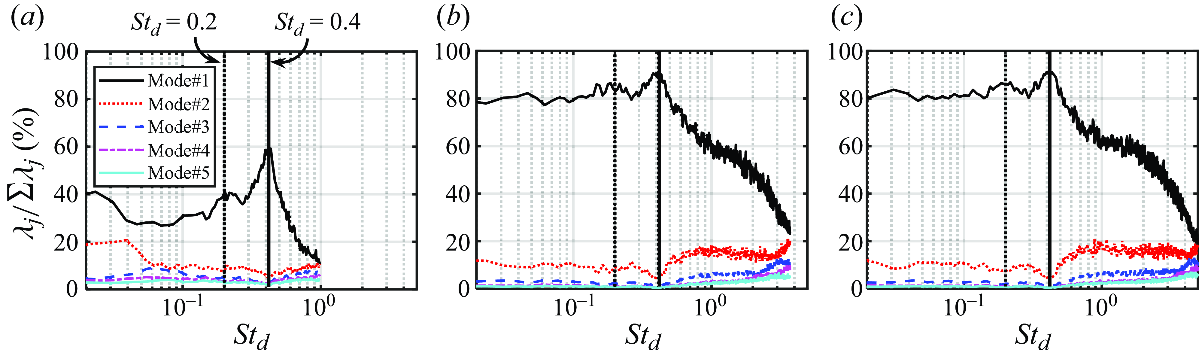
Figure 5. Effect of sampling rate on SPOD eigenspectra for the five leading modes. The eigenspectra for the 100, 375 and 500 kHz datasets are shown in (a), (b) and (c), respectively. The dotted and solid vertical lines represent $St_d$
= 0.2 and 0.42, respectively. Legend for each plot is the same and shown in (a).
$St_d$
= 0.2 and 0.42, respectively. Legend for each plot is the same and shown in (a).
Now consider the SPOD modes previously shown in figure 2. For the leading mode, the aliased energy along the wake centreline is negligible below approximately $St_d$
= 0.9 and therefore the symmetric wake instabilities revealed by the leading SPOD mode (figure 2
b) are indeed a feature of the flow. Despite the
$St_d$
= 0.9 and therefore the symmetric wake instabilities revealed by the leading SPOD mode (figure 2
b) are indeed a feature of the flow. Despite the $\kappa _x-f$
spectra for the second mode along the wake centreline (figure 4
b) being dominated by the aliased peak, the anti-symmetric instabilities revealed in the second SPOD mode (figure 2
c) are also real. This is because the anti-symmetry concentrates the largest SPOD eigenvector values away from the centreline and the
$\kappa _x-f$
spectra for the second mode along the wake centreline (figure 4
b) being dominated by the aliased peak, the anti-symmetric instabilities revealed in the second SPOD mode (figure 2
c) are also real. This is because the anti-symmetry concentrates the largest SPOD eigenvector values away from the centreline and the $\kappa _x-f$
spectra for SPOD eigenvectors along a horizontal trajectory cutting through the flow structures (not shown) show little influence of aliasing. However, the small-wavelength (large wavenumber) symmetrical structures in the wake at
$\kappa _x-f$
spectra for SPOD eigenvectors along a horizontal trajectory cutting through the flow structures (not shown) show little influence of aliasing. However, the small-wavelength (large wavenumber) symmetrical structures in the wake at $St_d$
= 0.80 (bottom row; figure 2
c) that resemble the primary instability of the wake are not real, but an artefact of aliasing in the schlieren imaging. These structures have a negative phase velocity since they are associated with peaks in the left half of the
$St_d$
= 0.80 (bottom row; figure 2
c) that resemble the primary instability of the wake are not real, but an artefact of aliasing in the schlieren imaging. These structures have a negative phase velocity since they are associated with peaks in the left half of the $\kappa _x-f$
spectra and these are the same structures that were misinterpreted as upstream propagating disturbances in our previous study (Awasthi et al. Reference Awasthi, McCreton, Moreau and Doolan2022). Lastly, we note that a wavenumber decomposition of the SPOD eigenvector along the wake centreline for the dataset used in figure 2 did not clearly show the double-peak
$\kappa _x-f$
spectra and these are the same structures that were misinterpreted as upstream propagating disturbances in our previous study (Awasthi et al. Reference Awasthi, McCreton, Moreau and Doolan2022). Lastly, we note that a wavenumber decomposition of the SPOD eigenvector along the wake centreline for the dataset used in figure 2 did not clearly show the double-peak $\kappa _x-f$
spectra discussed in the previous section. This is because the SPOD calculation used in figure 2 utilises the full fov of the 100 kHz dataset, whereas the spectra discussed in the previous section were calculated from the SPOD of light intensity fluctuations along the wake centreline.
$\kappa _x-f$
spectra discussed in the previous section. This is because the SPOD calculation used in figure 2 utilises the full fov of the 100 kHz dataset, whereas the spectra discussed in the previous section were calculated from the SPOD of light intensity fluctuations along the wake centreline.
3.4. Acoustic waves and their interactions in the wake
In this section we will show that, although the upstream travelling acoustic waves hypothesised by Awasthi et al. (Reference Awasthi, McCreton, Moreau and Doolan2022) are a measurement artefact, there are strong acoustic waves present in the cylinder wake that influence the wake dynamics and lead to an aeroacoustic resonance that manifests as vortex shedding in the wake. Unless otherwise stated, here, we will utilise the schlieren dataset for the 12 mm cylinder obtained with a flow-perpendicular knife-edge orientation which is more sensitive to wave-like features in this particular flow configuration (Awasthi et al. Reference Awasthi, McCreton, Moreau and Doolan2022). Figures 6(a) and 6(b) show the pixel variance in the schlieren images from the flow-parallel and flow-perpendicular knife-edge configurations, respectively. While these two images represent the same flow, they are markedly different from each other because they emphasise different features in the flow field. The flow-parallel knife-edge schlieren configuration (figure 6 a) is sensitive to the transverse gradient of density in the wake and emphasises smaller-scale, turbulent flow features. While the flow-perpendicular knife-edge schlieren configuration (figure 6 b) is sensitive to the streamwise density gradient and emphasises wave-like features in the flow. Momentarily, we will show that this is the reason why the variance image in figure 6 b shows significant unsteadiness in the outer regions of the wake and the free shear layers where acoustic-driven processes dominate the wake dynamics.

Figure 6. (a) Flow-parallel and (b) flow-perpendicular knife-edge schlieren variance images. The superimposed lines delineate the different wake flow features as described in Awasthi et al. (Reference Awasthi, McCreton, Moreau and Doolan2022). The variance along the wake centreline ( $y/d$
= 0) from the two imaging systems is shown in (c), while (d) shows the pixel light intensity fluctuation spectra along the wake centreline (
$y/d$
= 0) from the two imaging systems is shown in (c), while (d) shows the pixel light intensity fluctuation spectra along the wake centreline ( $y/d$
= 0) at
$y/d$
= 0) at $x/d$
= 2.36 (first peak), 2.52 (off-peak) and 2.58 (second peak).
$x/d$
= 2.36 (first peak), 2.52 (off-peak) and 2.58 (second peak).
Before we reveal the nature of the acoustic waves in the wake, an interesting observation from the variance images is shown in figure 6(c), which shows the variance along the wake centreline (normalised such that the maximum value is 1) from the two imaging systems. The flow-parallel knife-edge variance in the wake increases linearly with $x/d$
until the reattachment region where a plateau forms. Downstream of the reattachment the variance again increases as the wake develops and another plateau approximately between
$x/d$
until the reattachment region where a plateau forms. Downstream of the reattachment the variance again increases as the wake develops and another plateau approximately between $x/d$
= 2.1 and 2.35 is observed before a gradual decay. The flow-perpendicular knife-edge variance has a behaviour similar to that of the flow-parallel knife-edge curve until around
$x/d$
= 2.1 and 2.35 is observed before a gradual decay. The flow-perpendicular knife-edge variance has a behaviour similar to that of the flow-parallel knife-edge curve until around $x/d$
= 1.8, past which there are noticeable differences. The variance does not show a plateau in the early wake and small-amplitude peaks in the variance beginning around
$x/d$
= 1.8, past which there are noticeable differences. The variance does not show a plateau in the early wake and small-amplitude peaks in the variance beginning around $x/d$
= 2.35 are observed. Interestingly, the genesis of these peaks coincides with the beginning of the gradual decay in variance observed in the flow-parallel knife-edge variance. It is possible that these two phenomena together signal the beginning of the supersonic flow in the wake. To further investigate the reason behind the modulation of the variance in the flow-perpendicular knife-edge dataset, figure 6(d) plots the spectral density of the flow-perpendicular knife-edge schlieren pixel intensity fluctuations at the first two peak locations (
$x/d$
= 2.35 are observed. Interestingly, the genesis of these peaks coincides with the beginning of the gradual decay in variance observed in the flow-parallel knife-edge variance. It is possible that these two phenomena together signal the beginning of the supersonic flow in the wake. To further investigate the reason behind the modulation of the variance in the flow-perpendicular knife-edge dataset, figure 6(d) plots the spectral density of the flow-perpendicular knife-edge schlieren pixel intensity fluctuations at the first two peak locations ( $x/d$
= 2.36 and 2.58) and at the local minimum located between these two peaks. Based on these spectra, the increase in the variance at the peak locations is not a narrowband phenomenon. At the first peak location, the frequency spectrum shows a peak around
$x/d$
= 2.36 and 2.58) and at the local minimum located between these two peaks. Based on these spectra, the increase in the variance at the peak locations is not a narrowband phenomenon. At the first peak location, the frequency spectrum shows a peak around $St_d$
= 0.04, while at the second peak location an increase in fluctuating energy around
$St_d$
= 0.04, while at the second peak location an increase in fluctuating energy around $St_d$
= 0.39 can be observed. We will now show that the modulation of the centreline variance values in the flow-perpendicular knife-edge dataset is associated with disturbances that exist between the wake and the recompression shocks that form as a result of an interaction between acoustic waves, recompression shock and the voriticity in the wake.
$St_d$
= 0.39 can be observed. We will now show that the modulation of the centreline variance values in the flow-perpendicular knife-edge dataset is associated with disturbances that exist between the wake and the recompression shocks that form as a result of an interaction between acoustic waves, recompression shock and the voriticity in the wake.
Figure 7. Fourier modes of the upper half of the wake at $St_d$
= (a) 0.04 and (b) 0.39 extracted from the flow-perpendicular knife-edge schlieren images. The levels shown are spectral density values in each pixel in dB.
$St_d$
= (a) 0.04 and (b) 0.39 extracted from the flow-perpendicular knife-edge schlieren images. The levels shown are spectral density values in each pixel in dB.
Figures 7(a) and 7(b) plots the spectral density values in each pixel of the schlieren frame at $St_d$
= 0.04 and 0.39, respectively, from a flow-perpendicular knife-edge dataset taken at 50 kHz that captures only the upper half of the wake (referred to as the half-plane dataset from hereon). Given the limited fov of the schlieren set-up, this particular dataset shows more details of the flow around the recompression shock and momentarily we will utilise it to reveal the nature of the acoustic waves in the wake. These Fourier modes show that the largest fluctuating energy in the flow-perpendicular knife-edge schlieren dataset is concentrated around the recompression shock, outer regions of the wake and in the free stream between the wake and the recompression shock. The magnitude of the light intensity fluctuations in the wake is generally larger at
$St_d$
= 0.04 and 0.39, respectively, from a flow-perpendicular knife-edge dataset taken at 50 kHz that captures only the upper half of the wake (referred to as the half-plane dataset from hereon). Given the limited fov of the schlieren set-up, this particular dataset shows more details of the flow around the recompression shock and momentarily we will utilise it to reveal the nature of the acoustic waves in the wake. These Fourier modes show that the largest fluctuating energy in the flow-perpendicular knife-edge schlieren dataset is concentrated around the recompression shock, outer regions of the wake and in the free stream between the wake and the recompression shock. The magnitude of the light intensity fluctuations in the wake is generally larger at $St_d$
= 0.39, although the free shear layers at
$St_d$
= 0.39, although the free shear layers at $St_d$
= 0.04 show larger energy levels perhaps due to a coherent oscillation of the shear-layer/recompression shock system that was visible in the flow-parallel knife-edge schlieren SPOD modes (figure 2). The free-stream disturbances between the wake and the recompression shocks revealed in the Fourier modes here could either be a result of disturbances released from the recompression waves, or they could be associated with disturbances originating from the wake instabilities and terminating near the recompression waves. Regardless, we will now show that the free-stream region of the wake where these disturbances occur is dominated by an acoustic–vorticity interaction where the acoustic energy input is provided by Mach waves that originate in the free shear layer upstream of the reattachment location and then intensify as they interact with the recompression shocks.
$St_d$
= 0.04 show larger energy levels perhaps due to a coherent oscillation of the shear-layer/recompression shock system that was visible in the flow-parallel knife-edge schlieren SPOD modes (figure 2). The free-stream disturbances between the wake and the recompression shocks revealed in the Fourier modes here could either be a result of disturbances released from the recompression waves, or they could be associated with disturbances originating from the wake instabilities and terminating near the recompression waves. Regardless, we will now show that the free-stream region of the wake where these disturbances occur is dominated by an acoustic–vorticity interaction where the acoustic energy input is provided by Mach waves that originate in the free shear layer upstream of the reattachment location and then intensify as they interact with the recompression shocks.

Figure 8. Four consecutive instantaneous flow-perpendicular knife-edge schlieren images of the top half of the cylinder wake. The time between images is 0.02 ms and the dashed ellipse highlights the trajectory of the acoustic wave and the disturbance its interaction with the recompression shock generates. The approaching acoustic wave shown in (a) is distorted as it interacts with the recompression shock in (b) resulting in production of strong fluctuations downstream of the shock shown in (c) that are convected downstream as seen in (d). The dashed ovals in panels (a)–(d) track the same disturbance as it convects through the schlieren images. Panel (a) also shows the angle of the approaching Mach wave with respect to the local free-stream direction.
We now show that the cylinder wake consists of a strong acoustic waves that interact with the recompression shock wave to introduce new and significant disturbances into the wake. To do this, we will utilise the instantaneous flow-perpendicular knife-edge schlieren images from the half-plane dataset that was used to obtain the Fourier modes shown in figure 7. Figure 8 shows four consecutive, mean-subtracted instantaneous schlieren snapshots of the upper wake. For clarity, these images only show the positive values of mean-subtracted intensities and the images have been enhanced using an edge-aware local Laplacian filter and contrast enhancement. The dashed oval in each image tracks the same disturbance as it convects downstream.
Now consider the instantaneous schlieren snapshots in figure 8. In the first image in (a), a compression wave attached to disturbances in the shear layer and protruding into the free stream can be clearly seen upstream of the recompression shock. As this wave approaches the recompression shock in (b), it turns with the flow, is distorted and interacts with the recompression shock, releasing strong disturbances into the wake region, as seen in (c). The disturbances generated as a result of this interaction are then convected along with the wake, as seen in (d). A new compression wave approaching the shock and interacting with it can also be observed in (c) and (d), respectively. A visual inspection of several other instantaneous images revealed similar acoustic process occurring in the wake. These results show that in the cylinder wake the approaching free shear layers consist of strong acoustic waves that are amplified as they pass the recompression shock (an acoustic/shock interaction) and then interact with the wake vorticity (an acoustic/vorticity interaction). This latter interaction is likely responsible for the small-amplitude peaks observed in the flow-perpendicular knife-edge schlieren variance previously shown in figure 6(c). Lastly, we note that an examination of several instantaneous images such as those shown here also reveal that the instabilities in the wake consist of prominent $\Lambda$
-shaped structures that are highlighted in figures 8(b) and 8(c). The node of these structures is attached to the recompression shock and an analysis of the schlieren movies shows that the disturbances originating as a result of the acoustic-shock interaction is responsible for the formation of these structures.
$\Lambda$
-shaped structures that are highlighted in figures 8(b) and 8(c). The node of these structures is attached to the recompression shock and an analysis of the schlieren movies shows that the disturbances originating as a result of the acoustic-shock interaction is responsible for the formation of these structures.
The compression waves overriding the free shear layer, their interaction with the recompression shock and introduction of new disturbances towards the wake can also be clearly observed in the SPOD modes of the half-plane flow-perpendicular knife-edge schlieren datasets, as shown in figure 9. This figure shows the SPOD eigenspectra and the two leading modes at three different frequencies. The eigenspectra (figure 9
a) have a different appearance than their flow-parallel knife-edge schlieren counterpart (figure 2
a) in that they show nearly a white spectrum for $St_d\lt$
0.25 and only a single prominent peak around
$St_d\lt$
0.25 and only a single prominent peak around $St_d$
= 0.42 for the two most energetic modes. Given that the flow-perpendicular knife-edge schlieren is more sensitive to wave-like features in this particular flow configuration, the absence of the peak around
$St_d$
= 0.42 for the two most energetic modes. Given that the flow-perpendicular knife-edge schlieren is more sensitive to wave-like features in this particular flow configuration, the absence of the peak around $St_d$
= 0.2 and a prominent peak around
$St_d$
= 0.2 and a prominent peak around $St_d$
= 0.42 suggest that the former instability may be hydrodynamic in nature, while the latter is aeroacoustic in nature. Momentarily in § 3.5 we present low-order reconstruction of the wake based on inversion of SPOD modes that conclusively shows that this is indeed the case.
$St_d$
= 0.42 suggest that the former instability may be hydrodynamic in nature, while the latter is aeroacoustic in nature. Momentarily in § 3.5 we present low-order reconstruction of the wake based on inversion of SPOD modes that conclusively shows that this is indeed the case.
Considering now the two most energetic SPOD modes shown in figure 9(b–g) at three frequencies, we note that each mode here also shows oblique coherent structures that are associated with the compression waves and their interaction with the recompression shock and the wake vorticity as explained previously through the analysis of instantaneous schlieren images. These modes clearly show that the separated free shear layer consists of compression waves that intensify as they pass through the recompression shock. The leading mode at $St_d$
= 0.03 (figure 9
b) also shows a coherent oscillation of the shear layer and the recompression shock which is likely responsible for the low-frequency unsteadiness of the recompression shock, as discussed above in the discussion of flow-parallel knife-edge schlieren and also in the previous work (Awasthi et al. Reference Awasthi, McCreton, Moreau and Doolan2022). The compression waves at
$St_d$
= 0.03 (figure 9
b) also shows a coherent oscillation of the shear layer and the recompression shock which is likely responsible for the low-frequency unsteadiness of the recompression shock, as discussed above in the discussion of flow-parallel knife-edge schlieren and also in the previous work (Awasthi et al. Reference Awasthi, McCreton, Moreau and Doolan2022). The compression waves at $St_d$
= 0.03 and 0.2 (first two rows) are clearly attached to the shear-layer instabilities and have nearly the same inclination as the waves observed in the instantaneous images in figure 8. The waves at the shedding frequency (figures 9
f and 9
g) have a more defined structure and stronger spatial coherence, a strong indicator of the presence of aeroacoustic resonance. Interestingly, these waves have a shallower angle (approximately 50
$St_d$
= 0.03 and 0.2 (first two rows) are clearly attached to the shear-layer instabilities and have nearly the same inclination as the waves observed in the instantaneous images in figure 8. The waves at the shedding frequency (figures 9
f and 9
g) have a more defined structure and stronger spatial coherence, a strong indicator of the presence of aeroacoustic resonance. Interestingly, these waves have a shallower angle (approximately 50 $^\circ$
with respect to the free shear layer) compared with the compression waves at lower frequencies and those observed in the instantaneous images. This difference in the wave angle suggests that the waves at the shedding frequency have a different convection velocity than those at other frequencies. We will now undertake further analysis of these waves which suggests that the steeper waves observed at off-peak frequencies could be eddy Mach waves attached to the convective structures in the shear layer, whereas the shallower waves observed at the shedding frequency are acoustic waves that originate within the subsonic recirculation region behind the cylinder.
$^\circ$
with respect to the free shear layer) compared with the compression waves at lower frequencies and those observed in the instantaneous images. This difference in the wave angle suggests that the waves at the shedding frequency have a different convection velocity than those at other frequencies. We will now undertake further analysis of these waves which suggests that the steeper waves observed at off-peak frequencies could be eddy Mach waves attached to the convective structures in the shear layer, whereas the shallower waves observed at the shedding frequency are acoustic waves that originate within the subsonic recirculation region behind the cylinder.
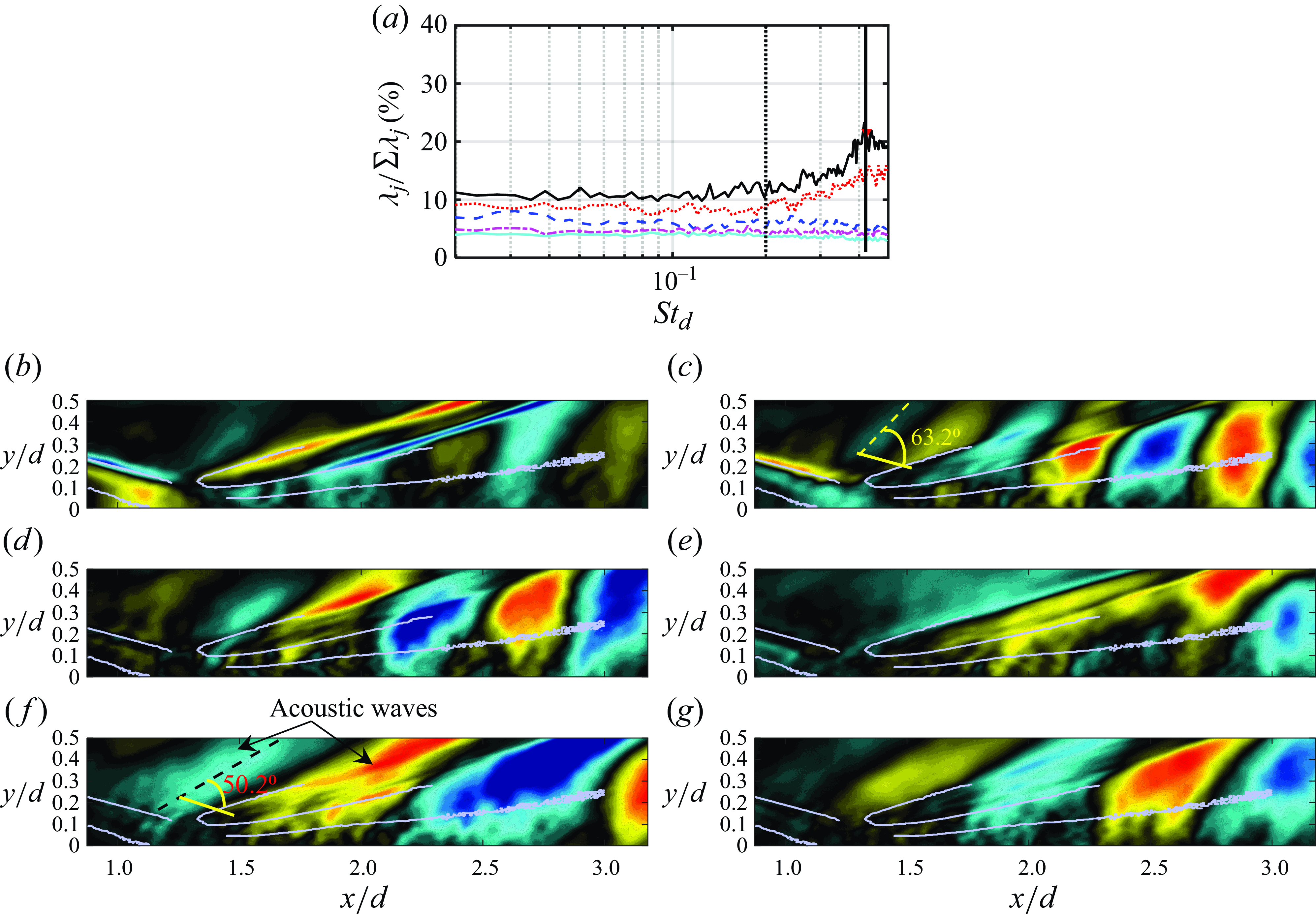
Figure 9. The SPOD of the half-plane focusing schlieren dataset using a flow-perpendicular knife-edge orientation. The SPOD eigenspectra for the five most energetic modes are shown in (a). The leading SPOD mode is shown in (b, d, f), while the second most energetic mode is shown in (c, e, g) for $St_d$
= 0.03 (b, c);
$St_d$
= 0.03 (b, c); $St_d$
= 0.2 (d, e);
$St_d$
= 0.2 (d, e); $St_d$
= 0.42 (f, g). The colour scale for each mode is the same as that shown in figure 2.
$St_d$
= 0.42 (f, g). The colour scale for each mode is the same as that shown in figure 2.
The compression waves attached to the approaching free shear layer observed in the raw schlieren images are reminiscent of the eddy Mach waves that have been documented in jet noise problems (Tam Reference Tam2009), compressible mixing layers (Rossmann, Mungal & Hanson Reference Rossmann, Mungal and Hanson2002) as well as supersonic boundary layers (Duan, Choudhari & Wu Reference Duan, Choudhari and Wu2014). Mach radiation in supersonic flows occurs when the velocity difference between the instabilities and the surrounding flow exceeds the local speed of sound and the near-field pressure field associated with the instabilities behaves like a wavy wall in supersonic flows (Tam Reference Tam2009). In what follows, we will derive some quantities associated with the Mach radiation in the free shear layers behind the cylinder and show that this radiation is particularly strong around $St_d$
= 0.42, further bolstering the argument that the vortex shedding in supersonic cylinder flows is driven by aeroacoustic processes.
$St_d$
= 0.42, further bolstering the argument that the vortex shedding in supersonic cylinder flows is driven by aeroacoustic processes.
The characteristic Mach number associated with Mach radiation is the convective Mach number which is defined as (Papamoschou & Roshko Reference Papamoschou and Roshko2006)
 \begin{equation} M_c = \frac {U_\infty -U_c}{a_\infty }, \end{equation}
where $U_c$
is the convection velocity of the eddies, and
$U_c$
is the convection velocity of the eddies, and $U_\infty$
and
$U_\infty$
and $a_\infty$
are the free-stream and acoustic wave velocities, respectively. The convective Mach number can be estimated by calculating the Mach angle of the acoustic waves. Going back to the instantaneous image of the compression wave radiating from the shear layer in figure 8(a), we note that the wave is steeper closer to the shear layer, likely due to a slightly higher temperature in this region which increases the local sound speed, resulting in a larger Mach angle. Further away from the shear layer, the wave angle with respect to the free stream (assumed to be parallel to the shear layer) is approximately 63
$a_\infty$
are the free-stream and acoustic wave velocities, respectively. The convective Mach number can be estimated by calculating the Mach angle of the acoustic waves. Going back to the instantaneous image of the compression wave radiating from the shear layer in figure 8(a), we note that the wave is steeper closer to the shear layer, likely due to a slightly higher temperature in this region which increases the local sound speed, resulting in a larger Mach angle. Further away from the shear layer, the wave angle with respect to the free stream (assumed to be parallel to the shear layer) is approximately 63 $^\circ$
, which corresponds to
$^\circ$
, which corresponds to $M_c$
= 1.12. Then, using the convective Mach number definition above and the free-stream conditions (
$M_c$
= 1.12. Then, using the convective Mach number definition above and the free-stream conditions ( $U_\infty$
= 604 m s–1 and
$U_\infty$
= 604 m s–1 and $a_\infty$
= 201 m s–1) yields a shear-layer convection velocity of approximately
$a_\infty$
= 201 m s–1) yields a shear-layer convection velocity of approximately $U_c$
= 379 m s–1, or
$U_c$
= 379 m s–1, or $U_c$
= 0.63
$U_c$
= 0.63 $U_\infty$
. This velocity is slightly lower than that of a free jet (
$U_\infty$
. This velocity is slightly lower than that of a free jet ( $U_c$
= 0.7
$U_c$
= 0.7 $U_\infty$
), but it is reasonable considering that the flow prior to reattachment undergoes an adverse pressure gradient. Applying this same analysis to the shallower waves with an angle of approximately 50
$U_\infty$
), but it is reasonable considering that the flow prior to reattachment undergoes an adverse pressure gradient. Applying this same analysis to the shallower waves with an angle of approximately 50 $^\circ$
at the shedding frequency observed in the SPOD modes (figure 9
f) yields
$^\circ$
at the shedding frequency observed in the SPOD modes (figure 9
f) yields $M_c$
= 1.3 and
$M_c$
= 1.3 and $U_c$
= 343 m s–1 (0.57
$U_c$
= 343 m s–1 (0.57 $U_\infty$
). This phase velocity is close to the speed of sound associated with the stagnation temperature values (
$U_\infty$
). This phase velocity is close to the speed of sound associated with the stagnation temperature values ( $T_0$
= 292 K) in the present work and suggests that these shallow waves at
$T_0$
= 292 K) in the present work and suggests that these shallow waves at $St_d$
= 0.42 could be acoustic waves that originate within the recirculation region behind the cylinder where the temperature ratio can approach 1.0.
$St_d$
= 0.42 could be acoustic waves that originate within the recirculation region behind the cylinder where the temperature ratio can approach 1.0.
To show that the shallow waves at $St_d$
= 0.42 discussed above are indeed acoustic waves originating from the recirculation region, we utilise the SPOD modes of a resized version of the flow-parallel knife-edge schlieren dataset at 100 kHz for which the results were presented earlier (see figure 2 and table 1). This particular dataset has a smaller fov in the streamwise direction, but a larger fov in the vertical direction. The resolution of this dataset is 380
$St_d$
= 0.42 discussed above are indeed acoustic waves originating from the recirculation region, we utilise the SPOD modes of a resized version of the flow-parallel knife-edge schlieren dataset at 100 kHz for which the results were presented earlier (see figure 2 and table 1). This particular dataset has a smaller fov in the streamwise direction, but a larger fov in the vertical direction. The resolution of this dataset is 380 $\times$
240 pixels. Figure 10 shows the most energetic SPOD modes from this dataset at four different frequencies. At the lowest frequency (figure 10
a), the shear-layer instabilities and the characteristic low-frequency unsteadiness of the recompression shock can be clearly observed. The mode at
$\times$
240 pixels. Figure 10 shows the most energetic SPOD modes from this dataset at four different frequencies. At the lowest frequency (figure 10
a), the shear-layer instabilities and the characteristic low-frequency unsteadiness of the recompression shock can be clearly observed. The mode at $St_d$
= 0.2 (figure 10
b) shows coherent structures being pushed out of the reattachment region without the presence of any noticeable acoustic disturbances, which again suggests that this instability is hydrodynamic in nature. A similar behaviour is observed at the highest frequency (figure 10
d) shown here. However, the mode at
$St_d$
= 0.2 (figure 10
b) shows coherent structures being pushed out of the reattachment region without the presence of any noticeable acoustic disturbances, which again suggests that this instability is hydrodynamic in nature. A similar behaviour is observed at the highest frequency (figure 10
d) shown here. However, the mode at $St_d$
= 0.42 (figure 10
c) shows a different behaviour to the modes at other frequencies with wave-like disturbances radiating outwards from the recirculation region, confirming that the shallow waves observed earlier in the flow-perpendicular knife-edge schlieren SPOD modes indeed originate from the recirculation region. These waves radiate outwards into the free stream where they have a larger energy and a very shallow angle (due to the larger Mach number in the free stream). Momentarily, through a low-order reconstruction of the wake obtained by inverting the SPOD modes, we will show how these acoustic waves evolve and interact with the wake vorticity (see § 3.5). Before we do that, we will now utilise the convection velocities of the convective and the acoustic modes calculated above to hypothesise a straightforward aeroacoustic resonance model that could possibly explain the shedding mechanism in supersonic cylinder wakes.
$St_d$
= 0.42 (figure 10
c) shows a different behaviour to the modes at other frequencies with wave-like disturbances radiating outwards from the recirculation region, confirming that the shallow waves observed earlier in the flow-perpendicular knife-edge schlieren SPOD modes indeed originate from the recirculation region. These waves radiate outwards into the free stream where they have a larger energy and a very shallow angle (due to the larger Mach number in the free stream). Momentarily, through a low-order reconstruction of the wake obtained by inverting the SPOD modes, we will show how these acoustic waves evolve and interact with the wake vorticity (see § 3.5). Before we do that, we will now utilise the convection velocities of the convective and the acoustic modes calculated above to hypothesise a straightforward aeroacoustic resonance model that could possibly explain the shedding mechanism in supersonic cylinder wakes.
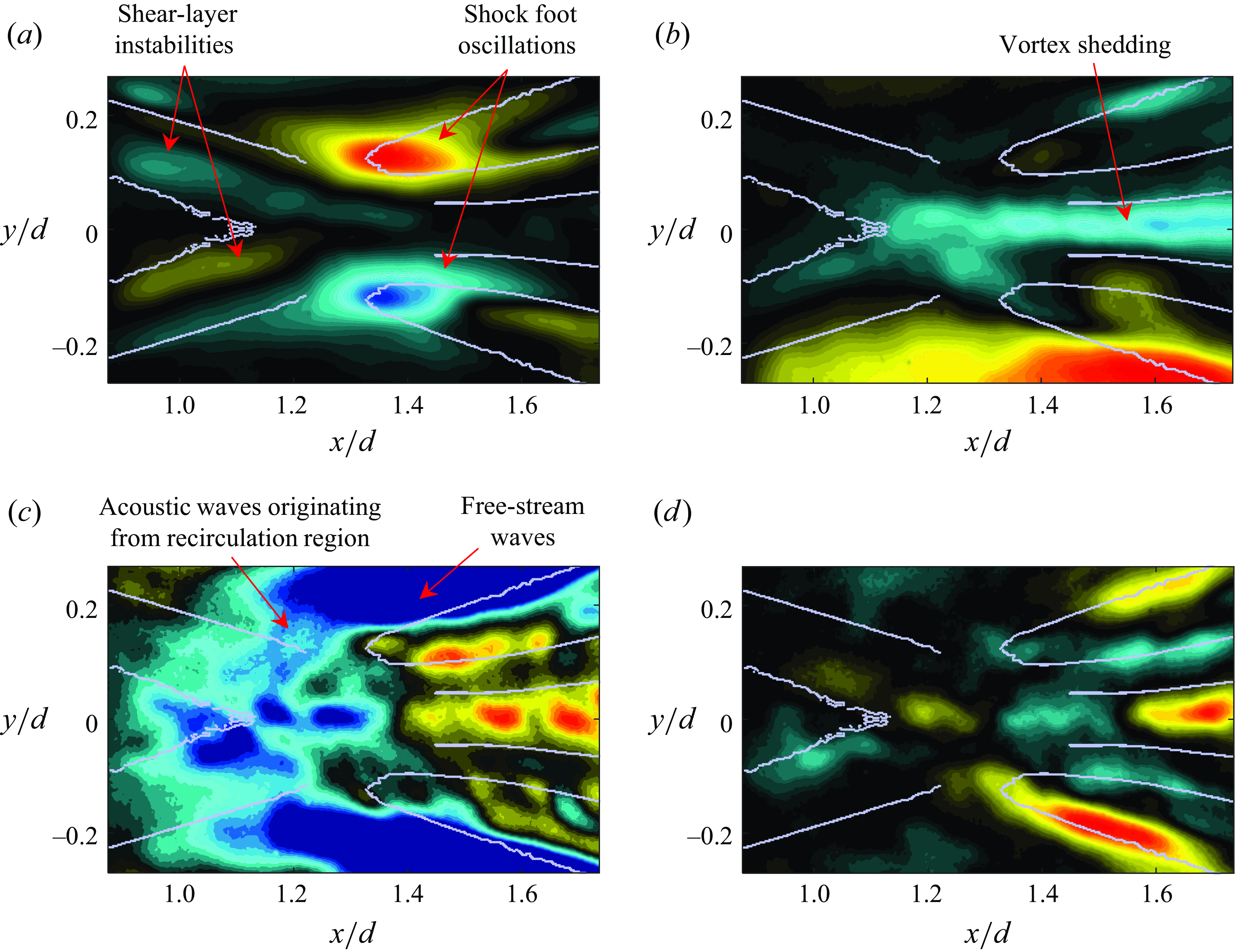
Figure 10. Leading SPOD modes from a resized flow-parallel knife-edge schlieren dataset at 100 kHz showing details of the flow in the shear layer and the recirculation region. The modes for four different frequencies are shown, $St_d$
= (a) 0.03, (b) 0.2, (c) 0.42 and (d) 0.80. The colour scale for each mode is the same as that shown in figure 2.
$St_d$
= (a) 0.03, (b) 0.2, (c) 0.42 and (d) 0.80. The colour scale for each mode is the same as that shown in figure 2.
It is apparent from the discussion thus far that the Mach radiation from the shear layer is an important feature of the cylinder wake. Since the flow in the recirculation region is subsonic, acoustic waves in this region will propagate upstream and can interact with the shear layer separating from the cylinder surface, thus creating an aeroacoustic feedback loop. The presence of an aeroacoustic feedback mechanism as the driver behind the vortex shedding in supersonic cylinder wakes has previously been hypothesised by Schmidt & Shepherd (Reference Schmidt and Shepherd2015), who have shown that the vortex shedding frequency scales on the length of sliplines in the free shear layers, suggesting that the separated flow region behind the cylinder may act as an acoustic resonator. Thus, one possible mechanism behind the vortex shedding in the wake is shown in figure 11(a). This image shows the edges of the salient flow features in the 12 mm cylinder wake as obtained through the edge-detection algorithm described in Awasthi et al. (Reference Awasthi, McCreton, Moreau and Doolan2022). After flow separation from the cylinder surface, the hydrodynamic instability propagates downstream with convection velocity, $U_c$
, generating acoustic waves on either side of the shear layers. The acoustic waves in the supersonic free stream can only travel in the downstream direction, but those trapped inside the separation bubble can propagate upstream (with phase velocity
$U_c$
, generating acoustic waves on either side of the shear layers. The acoustic waves in the supersonic free stream can only travel in the downstream direction, but those trapped inside the separation bubble can propagate upstream (with phase velocity $a_0$
) and disturb the shear layer at the separation point, closing the feedback loop.
$a_0$
) and disturb the shear layer at the separation point, closing the feedback loop.
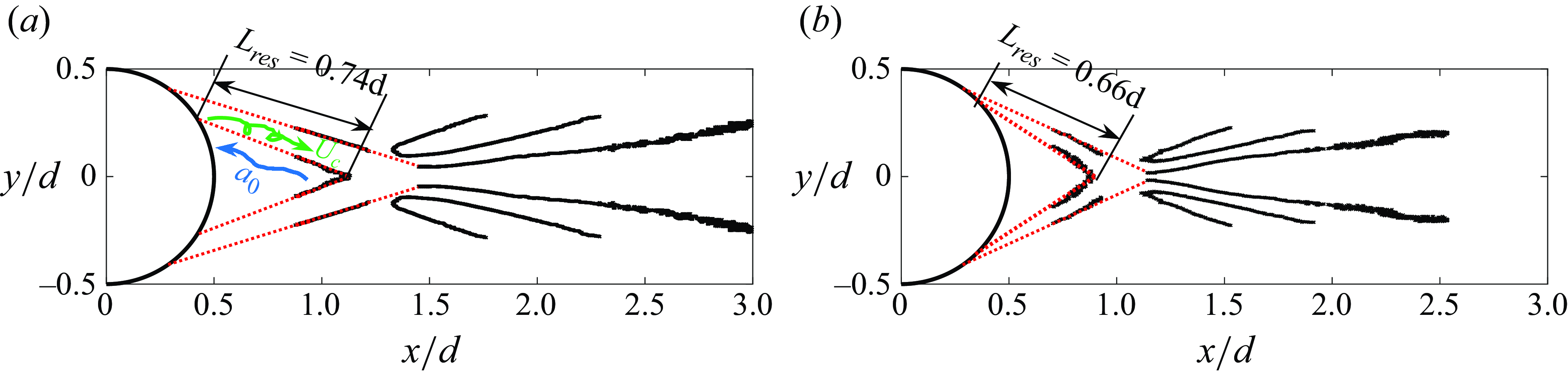
Figure 11. Aeroacoustic feedback mechanism and resonant length scale in the cylinder wake. The images in (a) and (b) show the edges of the salient features of the 12 and 15 mm cylinder wakes, respectively. The edges shown here were obtained by applying a custom edge-detection algorithm to the flow-parallel knife-edge schlieren variance images, see Awasthi et al. (Reference Awasthi, McCreton, Moreau and Doolan2022) for details.
The characteristic frequency associated with the feedback loop just described can be estimated if the propagation velocities of the two waves ( $U_c$
and
$U_c$
and $a_0$
) and the length of the loop (
$a_0$
) and the length of the loop ( $L_{res}$
) are known. The total period of the feedback loop (
$L_{res}$
) are known. The total period of the feedback loop ( $T_c$
) is given by
$T_c$
) is given by
 \begin{equation} T_c = T_d + T_u ,\end{equation}
where $T_d$
is the period of the downstream propagating KelvinHelmholtz instability and
$T_d$
is the period of the downstream propagating KelvinHelmholtz instability and $T_u$
is the period associated with the upstream propagating acoustic wave inside the recirculation region. From the loop period equation and noting that
$T_u$
is the period associated with the upstream propagating acoustic wave inside the recirculation region. From the loop period equation and noting that $T_d$
=
$T_d$
= $L_{res}/U_c$
and
$L_{res}/U_c$
and $T_u$
=
$T_u$
= $L_{res}/a_0$
, the loop characteristic frequency (
$L_{res}/a_0$
, the loop characteristic frequency ( $f_c$
) can be written in terms of the characteristic velocity of the upstream and downstream waves as
$f_c$
) can be written in terms of the characteristic velocity of the upstream and downstream waves as
 \begin{equation} f_c = \frac {U_c}{L_{res}(1+U_c/a_0)} .\end{equation}
This equation provides a way to estimate the shedding frequency in the wake under the assumption that it is a result of an interaction between the downstream propagating hydrodynamic instability and the upstream propagating acoustic waves trapped in the recirculation region. We will now use this equation to estimate the shedding frequency in the wake of the 12 mm cylinder, as well as the 15 mm cylinder which, although not considered here, exhibits shedding at $St_d$
= 0.44 (Awasthi et al. Reference Awasthi, McCreton, Moreau and Doolan2022). The shear-layer convection velocities for the two cylinders can be estimated using the Mach angle as explained earlier. The length scale,
$St_d$
= 0.44 (Awasthi et al. Reference Awasthi, McCreton, Moreau and Doolan2022). The shear-layer convection velocities for the two cylinders can be estimated using the Mach angle as explained earlier. The length scale, $L_{res}$
is taken to be the mean length of the shear layer that bounds the recirculation region, as depicted in figures 11(a) and 11(b) for the 12 and 15 mm diameter cylinders, respectively. Then, the only remaining unknown is the acoustic phase velocity in the recirculation region which, although not measured, can be approximated by assuming that the static temperature in this region approaches the stagnation temperature of the oncoming flow. Past measurements of the mean temperature field immediately behind a flat plate placed in a Mach 3 flow also support this assumption (Lachney & Clemens Reference Lachney and Clemens1998). Table 2 lists the time and length scales associated with the feedback loop for the two cylinders along with the estimated (
$L_{res}$
is taken to be the mean length of the shear layer that bounds the recirculation region, as depicted in figures 11(a) and 11(b) for the 12 and 15 mm diameter cylinders, respectively. Then, the only remaining unknown is the acoustic phase velocity in the recirculation region which, although not measured, can be approximated by assuming that the static temperature in this region approaches the stagnation temperature of the oncoming flow. Past measurements of the mean temperature field immediately behind a flat plate placed in a Mach 3 flow also support this assumption (Lachney & Clemens Reference Lachney and Clemens1998). Table 2 lists the time and length scales associated with the feedback loop for the two cylinders along with the estimated ( $f_c$
) and measured (
$f_c$
) and measured ( $f_{c_m}$
) shedding frequencies, where it can be seen that the estimated shedding frequency for both the cylinders shows a good agreement with the measurements. This further bolsters the original hypothesis of Schmidt & Shepherd (Reference Schmidt and Shepherd2015), derived using scaling argument, that vortex shedding in a supersonic cylinder wake could be a result of an aeroacoustic resonance that is driven by acoustic waves trapped within the subsonic recirculation region. Lastly, it is also worth noting that, although the feedback model described above yields reasonable estimates of the shedding frequencies in the wake, the present work does not provide direct evidence of the presence of this model due to the lack of flow visualisation closer to the cylinder surface. It is, of course, possible that similar to its low-speed counterpart the vortex shedding is a result of hydrodynamic instability. However, in the next section we do show that the vortex shedding around
$f_{c_m}$
) shedding frequencies, where it can be seen that the estimated shedding frequency for both the cylinders shows a good agreement with the measurements. This further bolsters the original hypothesis of Schmidt & Shepherd (Reference Schmidt and Shepherd2015), derived using scaling argument, that vortex shedding in a supersonic cylinder wake could be a result of an aeroacoustic resonance that is driven by acoustic waves trapped within the subsonic recirculation region. Lastly, it is also worth noting that, although the feedback model described above yields reasonable estimates of the shedding frequencies in the wake, the present work does not provide direct evidence of the presence of this model due to the lack of flow visualisation closer to the cylinder surface. It is, of course, possible that similar to its low-speed counterpart the vortex shedding is a result of hydrodynamic instability. However, in the next section we do show that the vortex shedding around $St_d$
= 0.42 is accompanied by strong acoustic waves, whereas the shedding around
$St_d$
= 0.42 is accompanied by strong acoustic waves, whereas the shedding around $St_d$
= 0.2 lacks these waves, suggesting the possibility that these two modes have different origins with the latter instability being hydrodynamic in nature (similar to the low-speed case).
$St_d$
= 0.2 lacks these waves, suggesting the possibility that these two modes have different origins with the latter instability being hydrodynamic in nature (similar to the low-speed case).
Table 2. Aeroacoustic feedback loop scales and estimated shedding frequency in the 12 and 15 mm cylinder wakes.
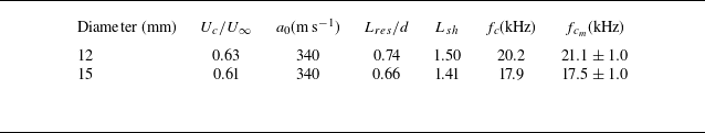
Although the aeroacoustic feedback model proposed here yields reasonable estimates of the shedding frequencies behind the cylinder, it is worth pointing out that there is some uncertainty associated with whether the loop length estimate ( $L_{res}$
) used here is the appropriate length scale. This is because the sonic lines within the shear layer along which the upstream propagation of acoustic waves occurs are not revealed by the schlieren images. In the analysis above it is implicitly assumed that the length
$L_{res}$
) used here is the appropriate length scale. This is because the sonic lines within the shear layer along which the upstream propagation of acoustic waves occurs are not revealed by the schlieren images. In the analysis above it is implicitly assumed that the length $L_{res}$
is the length of the sonic lines embedded within the shear layers, an assumption that may not be correct. It is, however, interesting to note that the convective wavelengths associated with the shear layer at the shedding frequency, estimated using the convection velocity (
$L_{res}$
is the length of the sonic lines embedded within the shear layers, an assumption that may not be correct. It is, however, interesting to note that the convective wavelengths associated with the shear layer at the shedding frequency, estimated using the convection velocity ( $U_c$
) and shown in table 2 as
$U_c$
) and shown in table 2 as $L_{sh}$
, are approximately 2
$L_{sh}$
, are approximately 2 $L_{res}$
and 2.1
$L_{res}$
and 2.1 $L_{res}$
for the 12 and 15 mm cylinders, respectively. This suggests that the resonant wavelength of the feedback loop is approximately twice the feedback path length. This situation resembles that of the formation of a standing wave in an open-ended duct where the anti-nodes (the points of maximum disturbance amplitude) are located at the extremities of the feedback path length. Thus, it is possible that the recirculation region bounded by the shear layers behind the cylinder which supports upstream propagating acoustic waves acts like an open duct which allows formation of standing waves responsible for the vortex shedding observed in the wake.
$L_{res}$
for the 12 and 15 mm cylinders, respectively. This suggests that the resonant wavelength of the feedback loop is approximately twice the feedback path length. This situation resembles that of the formation of a standing wave in an open-ended duct where the anti-nodes (the points of maximum disturbance amplitude) are located at the extremities of the feedback path length. Thus, it is possible that the recirculation region bounded by the shear layers behind the cylinder which supports upstream propagating acoustic waves acts like an open duct which allows formation of standing waves responsible for the vortex shedding observed in the wake.
In the work of Schmidt & Shepherd (Reference Schmidt and Shepherd2015), a universal Strouhal number of approximately 0.48 was obtained for the cylinder vortex shedding by using the sliplines that lie just outside the sonic lines as the length scales and the approaching free-stream velocity as the time scale. Considering their schlieren images, the sliplines appear to nearly coincide with the outer shear-layer boundary defined here, whereas we are taking the inner shear-layer boundary revealed by the schlieren image variance as the resonant length scale. This difference between the present work and that of Schmidt & Shepherd (Reference Schmidt and Shepherd2015) is reflected in the fact that the universal Strouhal number in the present work, obtained by manipulating equation (3.4) and using the approaching free-stream velocity as the time scale above is approximately 0.3, whereas in the previous work it is higher. It is, of course, possible that their results can be rescaled on a smaller, proportional length to yield the same universal Strouhal number as the present work. Thus, it remains unclear whether the choice of the feedback loop length in the present work is appropriate and further measurements, particularly closer to the cylinder surface, are required to fully characterise the resonant behaviour in the cylinder wake. Nonetheless, through a low-order modelling of the cylinder wake, we will now show that at the shedding frequency there are noticeable coherent structures that straddle the inner shear-layer boundary, which suggests that the length of this boundary could determine the vortex shedding frequency in the cylinder wake.
3.5. Low-order reconstruction of the cylinder wake
In this section, we briefly discuss the cylinder wake dynamics around the shedding frequency through a low-order reconstruction of the SPOD modes. The SPOD mode reconstruction was developed using the frequency-domain formulation discussed in Nekkanti & Schmidt (Reference Nekkanti and Schmidt2021) and it involves projecting an expansion coefficient matrix on the SPOD eigenvectors to obtain the original Fourier realisations which are then inverse Fourier transformed to reconstruct the flow snapshots. The reconstruction of the flow snapshots based on a specific mode (or a combination of modes that are orthogonal to each other) can be obtained by zeroing the rows of the expansion coefficient matrix (matrix A in Nekkanti & Schmidt (Reference Nekkanti and Schmidt2021)) that correspond to the modes to be rejected in the reconstruction. Since the SPOD modes are also orthogonal in time, the reconstruction can be carried out at a specific frequency (or frequencies) by retaining the expansion coefficients along the columns of the coefficient matrix that correspond to the frequency or frequencies of interest.
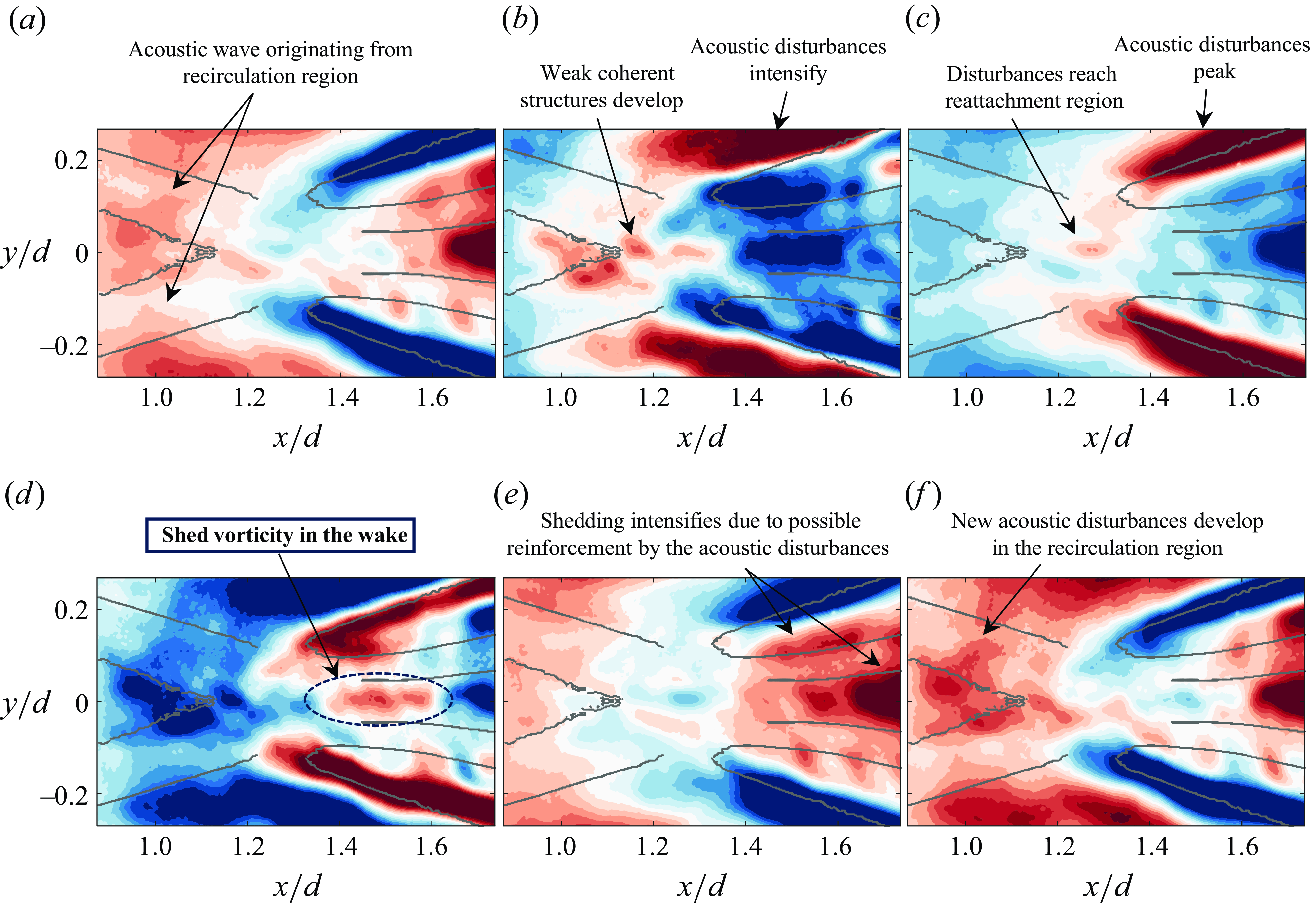
Figure 12. Low-order reconstruction of the flow-parallel knife-edge schlieren snapshots using the leading SPOD mode at $St_d$
= 0.42. Six consecutive instantaneous snapshots with
$St_d$
= 0.42. Six consecutive instantaneous snapshots with $\Delta t$
= 0.01 ms are shown. The negative, zero and positive values are represented by blue, white and red colours, respectively. For each reconstructed snapshot, 31 colour levels are shown between 50 % of the minimum and maximum of the value found within that snapshot.
$\Delta t$
= 0.01 ms are shown. The negative, zero and positive values are represented by blue, white and red colours, respectively. For each reconstructed snapshot, 31 colour levels are shown between 50 % of the minimum and maximum of the value found within that snapshot.
Figure 12 shows six consecutive instantaneous snapshots of the 12 mm cylinder wake reconstructed using the leading mode at the shedding frequency ( $St_d$
= 0.42). Here, we have utilised the same resized flow-parallel knife-edge schlieren dataset taken at 100 kHz for which SPOD modes were presented in figure 10. In order to enhance the image contrast and show the weaker structures clearly, 31 colour levels are shown between 50 % of the minimum and maximum of the reconstructed value found within each individual snapshot. Some noteworthy flow features have been highlighted above each snapshot. The six snapshots presented here show the complete cycle of the vortex shedding in the wake. Starting with the most upstream disturbances visible in (a), we can clearly see that there are disturbances radiating outwards from the recirculation region. These are the same shallow waves seen in the leading SPOD mode of the flow-perpendicular knife-edge schlieren dataset (see figure 9
f). These waves gain strength as they are accelerated in the free stream and approach the recompression shock, as shown in figure 12(b). At the same instant, weak coherent structures are released into the reattachment region, just downstream of the recirculation region. These coherent structures travel further downstream and appear to be weakly linked to the free-stream acoustic disturbances that peak in intensity as they interact with the recompression shock (figure 12
c). Finally, a clear discrete vortex is shed from the reattachment region into the wake, as shown in figure 12(d). At the same time instance, acoustic disturbances of opposite sign (associated with the trough of the wave) radiating from the recirculation region can also be observed.
$St_d$
= 0.42). Here, we have utilised the same resized flow-parallel knife-edge schlieren dataset taken at 100 kHz for which SPOD modes were presented in figure 10. In order to enhance the image contrast and show the weaker structures clearly, 31 colour levels are shown between 50 % of the minimum and maximum of the reconstructed value found within each individual snapshot. Some noteworthy flow features have been highlighted above each snapshot. The six snapshots presented here show the complete cycle of the vortex shedding in the wake. Starting with the most upstream disturbances visible in (a), we can clearly see that there are disturbances radiating outwards from the recirculation region. These are the same shallow waves seen in the leading SPOD mode of the flow-perpendicular knife-edge schlieren dataset (see figure 9
f). These waves gain strength as they are accelerated in the free stream and approach the recompression shock, as shown in figure 12(b). At the same instant, weak coherent structures are released into the reattachment region, just downstream of the recirculation region. These coherent structures travel further downstream and appear to be weakly linked to the free-stream acoustic disturbances that peak in intensity as they interact with the recompression shock (figure 12
c). Finally, a clear discrete vortex is shed from the reattachment region into the wake, as shown in figure 12(d). At the same time instance, acoustic disturbances of opposite sign (associated with the trough of the wave) radiating from the recirculation region can also be observed.
As the shed vortex propagates further into the wake (figure 12
e), it gains strength and it appears that it is being reinforced by the free-stream acoustic waves post interaction with the recompression shock. In our previous work (Awasthi et al. Reference Awasthi, McCreton, Moreau and Doolan2022), it was observed that the vortex shedding around $St_d$
= 0.42 did not become evident in the Fourier analysis of schlieren light intensity fluctuations until around
$St_d$
= 0.42 did not become evident in the Fourier analysis of schlieren light intensity fluctuations until around $x/d$
= 1.7. The snapshot in figure 12(e) here shows that a reinforcement of the shed vortices by the disturbances generated as a result of an interaction between the free-stream acoustic waves and the recompression shock may be responsible for this behaviour. This also suggests that, while the origin of the shedding in supersonic cylinder wakes may indeed be the aeroacoustic feedback loop within the recirculation region as proposed earlier, it is an interaction between the acoustic waves that are generated as a result of this feedback loop and the recompression shock that indirectly supports the prominence and persistence of the shedding behaviour observed in the wake. Finally, as the wake vortex exits the fov in figure 12(f), a new shedding cycle starting with waves radiating from the recirculation region can be observed. Note that the reconstructed flow field here did not show any clear evidence of upstream propagating acoustic waves within the recirculation region that could confirm the aeroacoustic feedback loop hypothesis presented in the previous section. This is likely due to both a limited schlieren fov that does not capture a large portion of the recirculation region and the weak nature of the acoustic disturbances.
$x/d$
= 1.7. The snapshot in figure 12(e) here shows that a reinforcement of the shed vortices by the disturbances generated as a result of an interaction between the free-stream acoustic waves and the recompression shock may be responsible for this behaviour. This also suggests that, while the origin of the shedding in supersonic cylinder wakes may indeed be the aeroacoustic feedback loop within the recirculation region as proposed earlier, it is an interaction between the acoustic waves that are generated as a result of this feedback loop and the recompression shock that indirectly supports the prominence and persistence of the shedding behaviour observed in the wake. Finally, as the wake vortex exits the fov in figure 12(f), a new shedding cycle starting with waves radiating from the recirculation region can be observed. Note that the reconstructed flow field here did not show any clear evidence of upstream propagating acoustic waves within the recirculation region that could confirm the aeroacoustic feedback loop hypothesis presented in the previous section. This is likely due to both a limited schlieren fov that does not capture a large portion of the recirculation region and the weak nature of the acoustic disturbances.
Finally, in this section we present the reconstruction of the flow field based on the leading SPOD at $St_d$
= 0.2 and show that this instability is hydrodynamic in nature and lacks the aeroacoustic forcing observed for
$St_d$
= 0.2 and show that this instability is hydrodynamic in nature and lacks the aeroacoustic forcing observed for $St_d$
= 0.42, the latter being the reason why the shedding at this frequency was found to rapidly decay as the wake develops in Awasthi et al. (Reference Awasthi, McCreton, Moreau and Doolan2022). Figure 13 shows six consecutive snapshots of the reconstructed flow field using the leading mode at
$St_d$
= 0.42, the latter being the reason why the shedding at this frequency was found to rapidly decay as the wake develops in Awasthi et al. (Reference Awasthi, McCreton, Moreau and Doolan2022). Figure 13 shows six consecutive snapshots of the reconstructed flow field using the leading mode at $St_d$
= 0.2. In the first panel (figure 13a), shear-layer instabilities approaching the reattachment region can be clearly observed. This is followed by the formation of coherent oscillations in the reattachment region and in the very early wake (figure 13
b–e). Weak compression waves radiating from these coherent structures can also be observed, along with shock ripples that were also discussed in Awasthi et al. (Reference Awasthi, McCreton, Moreau and Doolan2022). Finally, a new shedding cycle beginning with the shear-layer instabilities approaching the reattachment region can be seen in figure 13(f). Comparing the reconstructed flow field here with that at
$St_d$
= 0.2. In the first panel (figure 13a), shear-layer instabilities approaching the reattachment region can be clearly observed. This is followed by the formation of coherent oscillations in the reattachment region and in the very early wake (figure 13
b–e). Weak compression waves radiating from these coherent structures can also be observed, along with shock ripples that were also discussed in Awasthi et al. (Reference Awasthi, McCreton, Moreau and Doolan2022). Finally, a new shedding cycle beginning with the shear-layer instabilities approaching the reattachment region can be seen in figure 13(f). Comparing the reconstructed flow field here with that at $St_d$
= 0.42 in figure 12, we note the clear absence of any acoustic waves radiating from the recirculation region, as well as the intense free-stream acoustic disturbances and their interaction with the recompression shock. Although, a noticeably strong free-stream disturbance can be observed near the bottom of each image. This disturbance, however, is nearly parallel to the free stream and is not linked to the coherent structures within the recirculation region, shear layers or the wake. The origin of this disturbance is not clear, but it is possible that they are related to the oscillations of the separation shock that is generated as a result of flow separation on the cylinder surface, or these disturbances could be free-stream disturbances generated elsewhere in the facility.
$St_d$
= 0.42 in figure 12, we note the clear absence of any acoustic waves radiating from the recirculation region, as well as the intense free-stream acoustic disturbances and their interaction with the recompression shock. Although, a noticeably strong free-stream disturbance can be observed near the bottom of each image. This disturbance, however, is nearly parallel to the free stream and is not linked to the coherent structures within the recirculation region, shear layers or the wake. The origin of this disturbance is not clear, but it is possible that they are related to the oscillations of the separation shock that is generated as a result of flow separation on the cylinder surface, or these disturbances could be free-stream disturbances generated elsewhere in the facility.
The low-order representation of the cylinder wake in this section shows that the shedding mechanisms at $St_d$
= 0.2 and 0.42 are fundamentally different. The instability at
$St_d$
= 0.2 and 0.42 are fundamentally different. The instability at $St_d$
= 0.2 is the typical Kelvin–Helmholtz instability that is also observed in incompressible flow over a cylinder, while the instability at
$St_d$
= 0.2 is the typical Kelvin–Helmholtz instability that is also observed in incompressible flow over a cylinder, while the instability at $St_d$
= 0.42 is due to aeroacoustic resonance that develops within the recirculation region. The latter instability also emerges as the more dominant of the two, likely due to indirect acoustic input that is provided by an interaction between the recompression shock and the acoustic waves that form in the recirculation region as a result of the aeroacoustic resonance. On the other hand, the shedding at
$St_d$
= 0.42 is due to aeroacoustic resonance that develops within the recirculation region. The latter instability also emerges as the more dominant of the two, likely due to indirect acoustic input that is provided by an interaction between the recompression shock and the acoustic waves that form in the recirculation region as a result of the aeroacoustic resonance. On the other hand, the shedding at $St_d$
= 0.2 is weaker and decays rapidly in the wake due to a lack of an aeroacoustic feedback and presumably under the stabilising action of compressibility in the wake. A playback of the low-order reconstruction of the wake based on the leading SPOD mode at both
$St_d$
= 0.2 is weaker and decays rapidly in the wake due to a lack of an aeroacoustic feedback and presumably under the stabilising action of compressibility in the wake. A playback of the low-order reconstruction of the wake based on the leading SPOD mode at both $St_d$
= 0.2 and 0.42 that shows how the shedding evolves at these frequencies can be found in the supplementary material to this paper (see Movie 3 and Movie 4).
$St_d$
= 0.2 and 0.42 that shows how the shedding evolves at these frequencies can be found in the supplementary material to this paper (see Movie 3 and Movie 4).
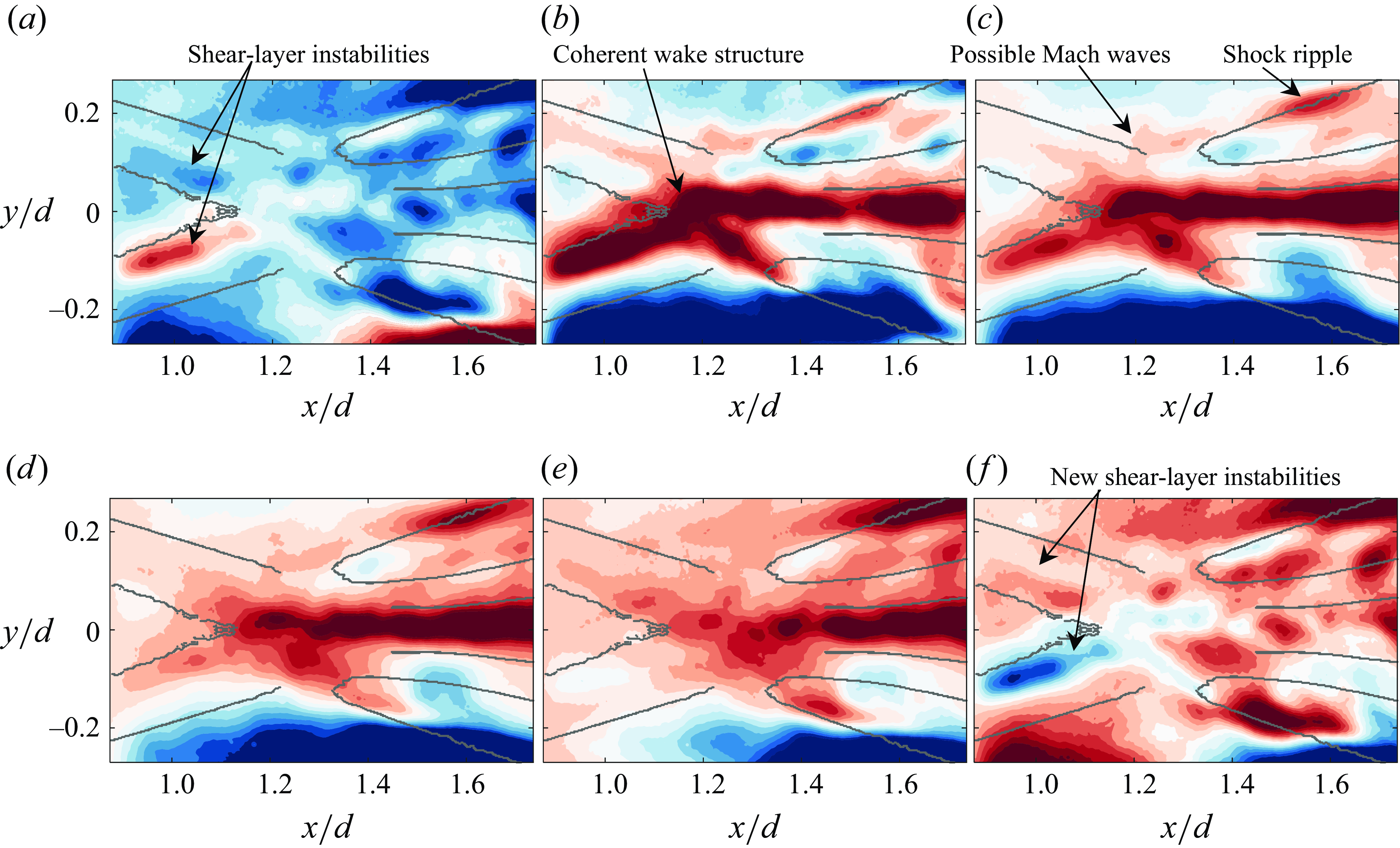
Figure 13. Low-order reconstruction of the flow-parallel knife-edge schlieren light intensity fluctuations using the leading SPOD mode at $St_d$
= 0.2. Six consecutive instantaneous snapshots with
$St_d$
= 0.2. Six consecutive instantaneous snapshots with $\Delta t$
= 0.01 ms are shown. Format of the figure is the same as figure 12.
$\Delta t$
= 0.01 ms are shown. Format of the figure is the same as figure 12.
4. Conclusion
Coherent structures in the wake of a 12 mm diameter circular cylinder placed in supersonic flow ( $M$
= 3.0) were studied through SPOD of high-speed focussing schlieren light intensity fluctuations. The Reynolds number based on the cylinder diameter was
$M$
= 3.0) were studied through SPOD of high-speed focussing schlieren light intensity fluctuations. The Reynolds number based on the cylinder diameter was $6.0 \times 10^5$
and schlieren images were acquired at different sampling rates up to 500 kHz. In this study, both horizontal and vertical knife-edge schlieren images, which correspond to the vertical and streamwise density gradients, respectively, were used to reveal several aspects of the flow field and aeroacoustic processes in the cylinder wake. Besides providing a detailed description of the cylinder wake summarised below, another major contribution of this work is that it provides a methodology based on wavenumber decomposition of SPOD eigenvectors that allows a clearer interpretation of the SPOD results, compared with an analysis of the SPOD mode shapes alone. The wavenumber analysis of the SPOD modes shows that what was previously believed to be an upstream propagating disturbance in the wake (Awasthi et al. Reference Awasthi, McCreton, Moreau and Doolan2022) is, in fact, an alias of the convective wake instability itself. Furthermore, the wavenumber analysis also shows that the wavepacket-like features in the wake that appear in lower-order SPOD modes could also be a subtle imaging artefact. It is shown that these wavepackets are a result of the modulation of the convective waveform by a wave whose wavelength is comparable to the streamwise field-of-view of the imaging system.
$6.0 \times 10^5$
and schlieren images were acquired at different sampling rates up to 500 kHz. In this study, both horizontal and vertical knife-edge schlieren images, which correspond to the vertical and streamwise density gradients, respectively, were used to reveal several aspects of the flow field and aeroacoustic processes in the cylinder wake. Besides providing a detailed description of the cylinder wake summarised below, another major contribution of this work is that it provides a methodology based on wavenumber decomposition of SPOD eigenvectors that allows a clearer interpretation of the SPOD results, compared with an analysis of the SPOD mode shapes alone. The wavenumber analysis of the SPOD modes shows that what was previously believed to be an upstream propagating disturbance in the wake (Awasthi et al. Reference Awasthi, McCreton, Moreau and Doolan2022) is, in fact, an alias of the convective wake instability itself. Furthermore, the wavenumber analysis also shows that the wavepacket-like features in the wake that appear in lower-order SPOD modes could also be a subtle imaging artefact. It is shown that these wavepackets are a result of the modulation of the convective waveform by a wave whose wavelength is comparable to the streamwise field-of-view of the imaging system.
The cylinder wake consists of both symmetric (varicose) and antisymmetric (sinuous) instability modes, with the former being dominant. The instabilities in the free shear layers that form after the flow separates from the cylinder surface radiate strong acoustic waves (eddy Mach waves) into the free stream that go on to interact with the recompression shocks, releasing significant disturbances that are then scattered by the wake vorticity. The low-frequency dynamics of the wake was found to be dominated by the recompression shock oscillations. The wake also shows a bimodal vortex shedding behaviour with noticeably larger energy around Strouhal numbers ( $St_d$
) of approximately 0.2 and 0.42. Through a low-order reconstruction of the flow field based on SPOD modes, it is shown that the shedding around
$St_d$
) of approximately 0.2 and 0.42. Through a low-order reconstruction of the flow field based on SPOD modes, it is shown that the shedding around $St_d$
= 0.2, similar to the low-speed case, is hydrodynamic in nature and decays rapidly as the wake is accelerated downstream of the reattachment point. On the other hand, the shedding around
$St_d$
= 0.2, similar to the low-speed case, is hydrodynamic in nature and decays rapidly as the wake is accelerated downstream of the reattachment point. On the other hand, the shedding around $St_d$
= 0.42, which is more prominent and persists farther into the wake, is aeroacoustic in nature. An aeroacoustic feedback loop model based on downstream propagating shear-layer instabilities and upstream propagating acoustic waves within the recirculation region is shown to accurately predict the vortex shedding frequency of this instability for two different diameter cylinders. Based on this model, the vortex shedding in supersonic cylinder wake occurs at a universal Strouhal number (based on the shear-layer length and approach free-stream velocity) of approximately 0.3. Although upstream propagating acoustic waves in the recirculation region that are responsible for closing the aeroacoustic feedback loop were not observed directly due to limited field-of-view and weak light intensity fluctuations, strong acoustic waves originating within the recirculation region and radiating into the free stream were clearly visible in the SPOD modes. These free-stream acoustic waves were found to be responsible for an indirect energy input into the early wake, which explains the persistence of the
$St_d$
= 0.42, which is more prominent and persists farther into the wake, is aeroacoustic in nature. An aeroacoustic feedback loop model based on downstream propagating shear-layer instabilities and upstream propagating acoustic waves within the recirculation region is shown to accurately predict the vortex shedding frequency of this instability for two different diameter cylinders. Based on this model, the vortex shedding in supersonic cylinder wake occurs at a universal Strouhal number (based on the shear-layer length and approach free-stream velocity) of approximately 0.3. Although upstream propagating acoustic waves in the recirculation region that are responsible for closing the aeroacoustic feedback loop were not observed directly due to limited field-of-view and weak light intensity fluctuations, strong acoustic waves originating within the recirculation region and radiating into the free stream were clearly visible in the SPOD modes. These free-stream acoustic waves were found to be responsible for an indirect energy input into the early wake, which explains the persistence of the $St_d$
= 0.42 shedding mode over the
$St_d$
= 0.42 shedding mode over the $St_d$
= 0.2 mode where no such waves exist (or are too weak).
$St_d$
= 0.2 mode where no such waves exist (or are too weak).
Supplementary movies
Supplementary movies are available at https://doi.org/10.1017/jfm.2025.10190.
Funding
This research was supported by the Australian Research Council under the Discovery Projects scheme (Grant ID: DP170101105).
Declaration of interests
The authors report no conflict of interest.
Appendix A. Spatio-temporal aliasing of schlieren images
In this section, we further explore and validate the temporal and spatial aliasing effects observed during the analysis of the modal wavenumber–frequency spectra discussed in § 3.2. Recall that these spectra showed a peak in the left half of the spectrum that was a function of the schlieren image acquisition frame rate, suggesting that this peak could be aliased energy corresponding to the frequencies greater than the Nyquist frequency. Here, we will further explore this negative wavenumber peak and show that it occurs because of insufficient image sampling rate. The SPOD wavenumber–frequency spectra also showed the presence of two parallel convective lobes in the second and third modes, with the spacing between these lobes being independent of the image acquisition rate, but the spectra for the third mode showed a larger spacing than that for the second mode. In this section, we will show that these double-peaked spectra are a function of the streamwise length of the schlieren fov (essentially the spatial sampling rate), and hence are an artefact of spatial aliasing in the schlieren images.
The temporal aliasing in the schlieren dataset follows directly from the Nyquist criterion and it is straightforward to show that the additional energy seen for the negative wavenumbers in § 3.2 is because of the folding of the spectra about the Nyquist frequency. For any time-resolved signal sampled at a frequency $\omega _s$
, the aliased frequency (
$\omega _s$
, the aliased frequency ( $\omega _a$
) is given by
$\omega _a$
) is given by
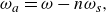 \begin{equation} \omega _a = \omega - n\omega _s ,\end{equation}
where $\omega$
is a frequency greater than the Nyquist frequency and
$\omega$
is a frequency greater than the Nyquist frequency and $n=0,1,2,3\ldots .$
is an integer multiple. Writing this equation in terms of the wavenumbers, we get
$n=0,1,2,3\ldots .$
is an integer multiple. Writing this equation in terms of the wavenumbers, we get
 \begin{equation} \kappa _a = \kappa U_c - n\omega _s ,\end{equation}
where $\kappa$
=
$\kappa$
= $2\pi f/U_c$
with
$2\pi f/U_c$
with $U_c$
being the characteristic velocity which in this case is the convection velocity of the turbulent structures in the wake (
$U_c$
being the characteristic velocity which in this case is the convection velocity of the turbulent structures in the wake ( $U_c$
= 0.72
$U_c$
= 0.72 $U_\infty$
). Then, rearranging we can write the difference between the convective wavenumber and the aliased wavenumber as
$U_\infty$
). Then, rearranging we can write the difference between the convective wavenumber and the aliased wavenumber as
 \begin{equation} \kappa -\kappa _a = n2\pi f_s/U_c ,\end{equation}
where $f_s$
is now the sampling rate in Hz. This equation yields the expected difference between the wavenumbers corresponding to the convective disturbances and the aliased energy and can be used to confirm that the negative wavenumber peaks observed in § 3.2 are, in fact, because of aliasing. To do this, the 500 kHz schlieren dataset was downsampled to create two additional datasets with a sampling frequency of 125 and 250 kHz. These datasets were then decomposed using SPOD and the modal wavenumber–frequency spectra corresponding to the most energetic SPOD eigenvector along the wake centreline were calculated for each dataset. Figure 14 shows these wavenumber spectra at four different frequencies. Note that, because of the sampling rate limitations, the spectra corresponding to the downsampled 125 kHz dataset is only shown at 55 kHz (figure 14
a) and at 245 kHz (figure 14
d) only the spectra from the original 500 kHz dataset is shown. Considering these plots we note that, even when the same dataset is downsampled, peaks at negative wavenumbers appear for lower sampling rate, confirming that the energy seen in the left half of the wavenumber–frequency spectrum is indeed due to temporal aliasing. The spectrum at 55 kHz only shows the aliased peak for the lowest sampling rate, while at 110 and 120 kHz, the 250 kHz dataset also shows these peaks. Finally, at sufficiently high frequency (245 kHz), the original 500 kHz also shows the aliased peak. To further confirm that the peaks for
$f_s$
is now the sampling rate in Hz. This equation yields the expected difference between the wavenumbers corresponding to the convective disturbances and the aliased energy and can be used to confirm that the negative wavenumber peaks observed in § 3.2 are, in fact, because of aliasing. To do this, the 500 kHz schlieren dataset was downsampled to create two additional datasets with a sampling frequency of 125 and 250 kHz. These datasets were then decomposed using SPOD and the modal wavenumber–frequency spectra corresponding to the most energetic SPOD eigenvector along the wake centreline were calculated for each dataset. Figure 14 shows these wavenumber spectra at four different frequencies. Note that, because of the sampling rate limitations, the spectra corresponding to the downsampled 125 kHz dataset is only shown at 55 kHz (figure 14
a) and at 245 kHz (figure 14
d) only the spectra from the original 500 kHz dataset is shown. Considering these plots we note that, even when the same dataset is downsampled, peaks at negative wavenumbers appear for lower sampling rate, confirming that the energy seen in the left half of the wavenumber–frequency spectrum is indeed due to temporal aliasing. The spectrum at 55 kHz only shows the aliased peak for the lowest sampling rate, while at 110 and 120 kHz, the 250 kHz dataset also shows these peaks. Finally, at sufficiently high frequency (245 kHz), the original 500 kHz also shows the aliased peak. To further confirm that the peaks for $\kappa _x\lt 0$
seen here for lower sampling rates are indeed due to aliasing, each plot also shows the wavenumber difference between the convective peak for
$\kappa _x\lt 0$
seen here for lower sampling rates are indeed due to aliasing, each plot also shows the wavenumber difference between the convective peak for $\kappa _x\gt 0$
and the aliased peak for
$\kappa _x\gt 0$
and the aliased peak for $\kappa _x\lt 0$
. The theoretical wavenumber difference obtained using equation (4.3) for the most energetic aliased peak (
$\kappa _x\lt 0$
. The theoretical wavenumber difference obtained using equation (4.3) for the most energetic aliased peak ( $n=1$
) are 1806 rad m−1, 3612 rad m−1 and 7224 rad m−1 for 125, 250 and 500 kHz datasets, respectively. These values are approximately the same as those observed in the wavenumber spectra in figure 14 for different sampling rates confirming the presence of aliased energy in the schlieren datasets.
$n=1$
) are 1806 rad m−1, 3612 rad m−1 and 7224 rad m−1 for 125, 250 and 500 kHz datasets, respectively. These values are approximately the same as those observed in the wavenumber spectra in figure 14 for different sampling rates confirming the presence of aliased energy in the schlieren datasets.

Figure 14. Leading SPOD mode wavenumber spectra along the wake centreline for three different sampling rates obtained by downsampling the same dataset (500 kHz dataset). The wavenumber spectra are shown for four different frequencies listed above each plot. The wavenumber difference between the convective and aliased peak is shown on each plot and the legend is shown at the bottom of the figure. The theoretical wavenumber difference for the 125, 250 and 500 kHz datasets are 1806, 3612 and 7224 rad m−1, respectively .
Finally, in this section we reveal the source of the double-peaked $\kappa _x - f$
spectra corresponding to the lower order SPOD modes presented in § 3.2. We will show that these spectra represent wavepacket-type features in the SPOD mode shapes whose wavelength is a function of the streamwise fov of the camera, and therefore are an imaging artefact and not actual flow features. In the analysis that follows, we will utilise the 375 kHz horizontal knife-edge schlieren dataset (see Table 1 for the specifications of this dataset). First consider figure 15 which shows the wavenumber spectra corresponding to the second and third SPOD modes along the wake centreline (which show the double-peak behaviour) at a constant frequency of 50 kHz. Here, the top row compares the wavenumber spectra along the wake centreline for the full dataset (1024 pixels in the streamwise direction) with those obtained by halving the spatial resolution of the same dataset (i.e. by reducing the spatial sampling frequency by half). The spectra for both sampling rates are identical, showing that the double-peak behaviour is not due to spatial aliasing. However, the wavelength of the two peaks in the spectra and the wavenumber spacing between them is a function of the streamwise fov of the schlieren images as shown in figure 15(c) and (d). These plots compare the spectra from the full dataset to those obtained by trimming the fov by half (512 pixels in the streamwise direction). Note that this trimmed dataset was obtained by a symmetric truncation of the full fov, i.e. by removing 256 pixels from either side of the images. Reducing the fov increases and decreases the wavenumbers corresponding to the right and left peaks, respectively, essentially spreading them apart and increasing the wavenumber separation between them. This shows that, although the double-peak behaviour is not a result of spatial aliasing in a conventional sense, it is indeed an imaging artefact related to the fov of the schlieren images. The remaining discussion in this appendix is dedicated to further understanding the origin of the double-peaked wavenumber spectra.
$\kappa _x - f$
spectra corresponding to the lower order SPOD modes presented in § 3.2. We will show that these spectra represent wavepacket-type features in the SPOD mode shapes whose wavelength is a function of the streamwise fov of the camera, and therefore are an imaging artefact and not actual flow features. In the analysis that follows, we will utilise the 375 kHz horizontal knife-edge schlieren dataset (see Table 1 for the specifications of this dataset). First consider figure 15 which shows the wavenumber spectra corresponding to the second and third SPOD modes along the wake centreline (which show the double-peak behaviour) at a constant frequency of 50 kHz. Here, the top row compares the wavenumber spectra along the wake centreline for the full dataset (1024 pixels in the streamwise direction) with those obtained by halving the spatial resolution of the same dataset (i.e. by reducing the spatial sampling frequency by half). The spectra for both sampling rates are identical, showing that the double-peak behaviour is not due to spatial aliasing. However, the wavelength of the two peaks in the spectra and the wavenumber spacing between them is a function of the streamwise fov of the schlieren images as shown in figure 15(c) and (d). These plots compare the spectra from the full dataset to those obtained by trimming the fov by half (512 pixels in the streamwise direction). Note that this trimmed dataset was obtained by a symmetric truncation of the full fov, i.e. by removing 256 pixels from either side of the images. Reducing the fov increases and decreases the wavenumbers corresponding to the right and left peaks, respectively, essentially spreading them apart and increasing the wavenumber separation between them. This shows that, although the double-peak behaviour is not a result of spatial aliasing in a conventional sense, it is indeed an imaging artefact related to the fov of the schlieren images. The remaining discussion in this appendix is dedicated to further understanding the origin of the double-peaked wavenumber spectra.
Figure 15. Wavenumber spectra along the wake centreline corresponding to the second (left) and third (right) SPOD modes at 50 kHz extracted from the 375 kHz dataset by varying the spatial resolution (top row) and the size of the fov in the streamwise direction (bottom row).
To understand why changing the fov in the streamwise direction affects the behaviour of the lower-order SPOD modes, we first need to determine what these double-peaked spectra represent. Figure 16(a) and (b) show the second and third SPOD modes, respectively, at $St_d$
= 2.0 for the 375 kHz dataset. Both these modes show multiple coherent structures that resemble the convective wake instabilities, but they are interspersed by regions of low energy, giving the modes the appearance of wavepackets (this is more obvious in the third SPOD mode in Figure 16(b), where the separation between the packets is large). Note that the temporal aliasing magnitude at this frequency is significantly lower than the main-lobe strength (
$St_d$
= 2.0 for the 375 kHz dataset. Both these modes show multiple coherent structures that resemble the convective wake instabilities, but they are interspersed by regions of low energy, giving the modes the appearance of wavepackets (this is more obvious in the third SPOD mode in Figure 16(b), where the separation between the packets is large). Note that the temporal aliasing magnitude at this frequency is significantly lower than the main-lobe strength ( $\lt$
10 dB) which ensures minimal influence of schlieren frame rate on the results. The presence of the wavepackets in these modes, along with the fact that the two parallel lobes in the
$\lt$
10 dB) which ensures minimal influence of schlieren frame rate on the results. The presence of the wavepackets in these modes, along with the fact that the two parallel lobes in the $\kappa _x-f$
spectra for these modes have the same group velocity (same slope) as the wake instabilities in the leading SPOD mode (see figure 4), suggests that these lower-order modes represent a modulated version of the convective waveform. Upon a closer inspection of the
$\kappa _x-f$
spectra for these modes have the same group velocity (same slope) as the wake instabilities in the leading SPOD mode (see figure 4), suggests that these lower-order modes represent a modulated version of the convective waveform. Upon a closer inspection of the $\kappa _x-f$
spectra previously shown in figure 4, we also note that the two wavenumber peaks in the lower modes are offset from the convective lobe that is present in the spectra for the leading SPOD mode by nearly a constant wavenumber in the left and right directions. Mathematically, these modulated waveforms can then be represented using the following wave equation:
$\kappa _x-f$
spectra previously shown in figure 4, we also note that the two wavenumber peaks in the lower modes are offset from the convective lobe that is present in the spectra for the leading SPOD mode by nearly a constant wavenumber in the left and right directions. Mathematically, these modulated waveforms can then be represented using the following wave equation:
 \begin{equation} W_I(\omega ,\kappa _x,x) = exp[i(\kappa _c+\kappa _0)x]+exp[i(\kappa _c-\kappa _0)x], \end{equation}
here, $\kappa _c = \omega /U_c$
is the convective wavenumber and
$\kappa _c = \omega /U_c$
is the convective wavenumber and $\kappa _0$
is the wavenumber of a wave which modulates the convective waveform. This equation is essentially a superposition of two waveforms each of which is a spatially modulated version of the convective wave propagating downstream with velocity
$\kappa _0$
is the wavenumber of a wave which modulates the convective waveform. This equation is essentially a superposition of two waveforms each of which is a spatially modulated version of the convective wave propagating downstream with velocity $U_c$
. Note that, in this equation, only the convective wavenumber depends on the frequency, while the wavelength of the modulating waveform is constant, suggesting that the modulating wave is not flow related. To conclusively show that this wave equation represents the wavepackets seen in the second and third SPOD modes, Figure 16(c) and (d) shows the SPOD eigenvector waveform along the wake centreline for the second and third modes, respectively, along with the waveform obtained using equation (4.4) scaled on the maximum value of the corresponding SPOD eigenvector for the sake of comparison. The reasons behind the choice of the wavenumbers for the modulating waveform (
$U_c$
. Note that, in this equation, only the convective wavenumber depends on the frequency, while the wavelength of the modulating waveform is constant, suggesting that the modulating wave is not flow related. To conclusively show that this wave equation represents the wavepackets seen in the second and third SPOD modes, Figure 16(c) and (d) shows the SPOD eigenvector waveform along the wake centreline for the second and third modes, respectively, along with the waveform obtained using equation (4.4) scaled on the maximum value of the corresponding SPOD eigenvector for the sake of comparison. The reasons behind the choice of the wavenumbers for the modulating waveform ( $\kappa _0$
) used here for the simulations is discussed below, but for now we note that the simulated waveforms accurately describe the mode shapes, showing that the wavepackets are a result of superposition of two waves with each wave being a modulated version of the convective waveform.
$\kappa _0$
) used here for the simulations is discussed below, but for now we note that the simulated waveforms accurately describe the mode shapes, showing that the wavepackets are a result of superposition of two waves with each wave being a modulated version of the convective waveform.
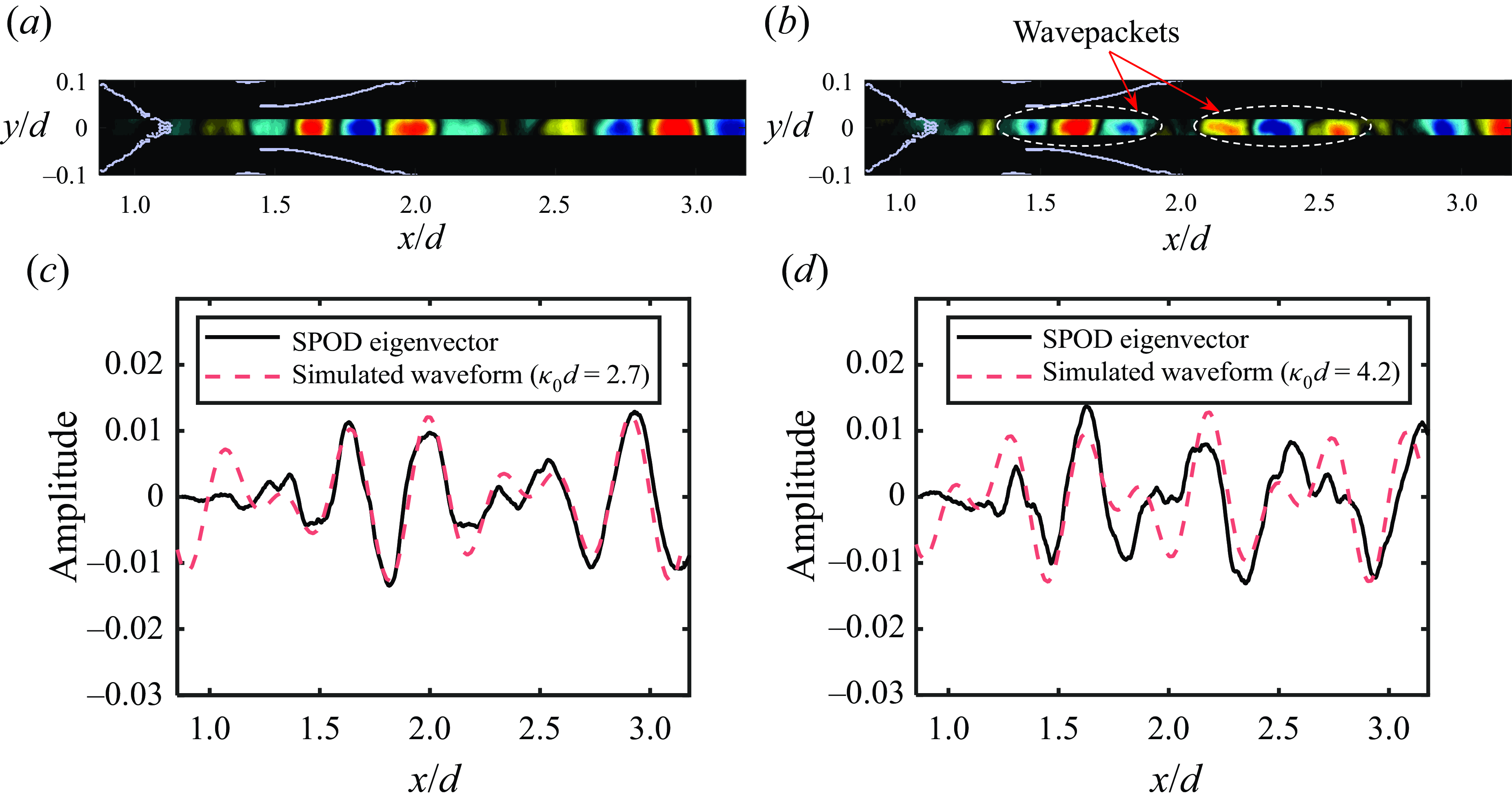
Figure 16. Wavepackets in lower-order SPOD modes at $St_d$
= 2.0 from the 375 kHz schlieren dataset. The second and third SPOD mode at
$St_d$
= 2.0 from the 375 kHz schlieren dataset. The second and third SPOD mode at $St_d$
= 2.0 are shown in (a) and (b), respectively. A comparison between the SPOD eigenvectors along the wake centreline and the simulated waveforms of equation (4.4) for the second and third modes are shown in (c) and (d), respectively. The magnitude of the simulated waveform has been scaled on the maximum value of SPOD eigenvector to enable comparison.
$St_d$
= 2.0 are shown in (a) and (b), respectively. A comparison between the SPOD eigenvectors along the wake centreline and the simulated waveforms of equation (4.4) for the second and third modes are shown in (c) and (d), respectively. The magnitude of the simulated waveform has been scaled on the maximum value of SPOD eigenvector to enable comparison.
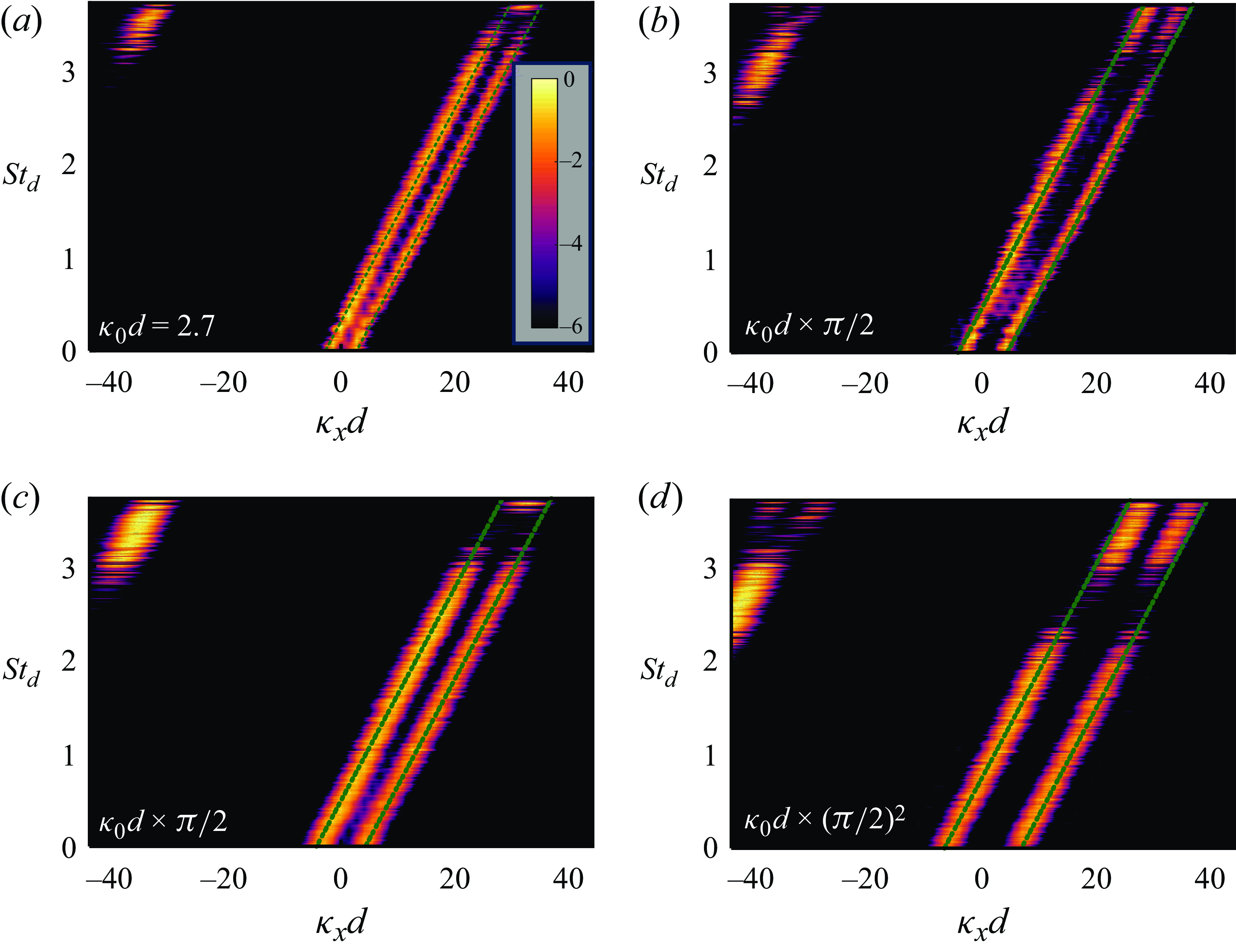
Figure 17. Wavenumberfrequency spectra of the second (left column) and third (right column) SPOD modes along the wake centreline from the 375 kHz dataset. The two parallel broken lines in each plot show the Fourier transform of equation (4.4) with the wavelength of the modulating waveform ( $\kappa _0$
) shown at the bottom-left in each plot. The spectra for the full fov (1024 pixels in the streamwise direction) are shown in (a) and (b), while those of the fov reduced by a factor of 2 (512 pixels) are shown in (c) and (d). The colour scale for each plot is the same and shown in (a).
$\kappa _0$
) shown at the bottom-left in each plot. The spectra for the full fov (1024 pixels in the streamwise direction) are shown in (a) and (b), while those of the fov reduced by a factor of 2 (512 pixels) are shown in (c) and (d). The colour scale for each plot is the same and shown in (a).
Now that we have established that the double-peaked $\kappa _x-f$
spectra represent wavepackets which themselves are a result of the convective instabilities being modulated by a wave with a constant wavelength, we can further investigate the origin of these structures by considering the wavelength of the modulating wave (
$\kappa _x-f$
spectra represent wavepackets which themselves are a result of the convective instabilities being modulated by a wave with a constant wavelength, we can further investigate the origin of these structures by considering the wavelength of the modulating wave ( $\kappa _0$
in equation (4.4)) that describes these wavepackets. Recall that we had already shown in figure 15(c) and (d) that the double-peaked wavenumber spectra are a function of the size of the streamwise fov of the schlieren images. The wavenumber corresponding to the streamwise fov size is
$\kappa _0$
in equation (4.4)) that describes these wavepackets. Recall that we had already shown in figure 15(c) and (d) that the double-peaked wavenumber spectra are a function of the size of the streamwise fov of the schlieren images. The wavenumber corresponding to the streamwise fov size is $\kappa _0d$
= 2.7 which, as shown in figure 16(c), describes the second mode SPOD eigenvector accurately. Interestingly, the modulating wavenumber corresponding to the wavepackets in third mode (
$\kappa _0d$
= 2.7 which, as shown in figure 16(c), describes the second mode SPOD eigenvector accurately. Interestingly, the modulating wavenumber corresponding to the wavepackets in third mode ( $\kappa _0d$
= 4.2) is approximately
$\kappa _0d$
= 4.2) is approximately $\pi /2$
times the wavenumber associated with the fov size, implying that the wavepackets in the third mode are not a harmonic of those in the second mode. This situation is further illustrated in figure 17(a) and (b), which shows the
$\pi /2$
times the wavenumber associated with the fov size, implying that the wavepackets in the third mode are not a harmonic of those in the second mode. This situation is further illustrated in figure 17(a) and (b), which shows the $\kappa _x-f$
spectra for the second and third SPOD modes, respectively, from the full fov 375 kHz dataset. The parallel broken lines overlaid on each plot represent the Fourier transform of equation (4.4) with the wavenumber of the modulating wave (
$\kappa _x-f$
spectra for the second and third SPOD modes, respectively, from the full fov 375 kHz dataset. The parallel broken lines overlaid on each plot represent the Fourier transform of equation (4.4) with the wavenumber of the modulating wave ( $\kappa _0$
) shown in the bottom-left corner. These plots confirm our previous observation that the wavepackets in the lower-order modes are due to modulation of convective instabilities, with the wavelength of the modulating waveform in the second mode being equal to the fov size in the streamwise direction, while the modulation wavelength in the third mode is
$\kappa _0$
) shown in the bottom-left corner. These plots confirm our previous observation that the wavepackets in the lower-order modes are due to modulation of convective instabilities, with the wavelength of the modulating waveform in the second mode being equal to the fov size in the streamwise direction, while the modulation wavelength in the third mode is $\pi /2$
times that.
$\pi /2$
times that.
Finally, we note that while the modulation wavelength corresponding to the second SPOD mode may be governed by the fov size in the streamwise direction, a reduction in the fov of the same dataset does not scale the modulation wavelength proportionally. This is shown in figure 17(c) and (d) which shows the $\kappa _x-f$
spectra for the second and third SPOD modes, respectively from the dataset obtained by reducing the fov of the original dataset by half. Note that this is the same dataset for wavenumber spectra at a single frequency were previously shown in figure 15(c) and (d). Further note that to obtain these spectra for the reduced fov, the SPOD eigenvectors were zero padded prior to Fourier transform to yield the same wavenumber resolution as the original dataset (
$\kappa _x-f$
spectra for the second and third SPOD modes, respectively from the dataset obtained by reducing the fov of the original dataset by half. Note that this is the same dataset for wavenumber spectra at a single frequency were previously shown in figure 15(c) and (d). Further note that to obtain these spectra for the reduced fov, the SPOD eigenvectors were zero padded prior to Fourier transform to yield the same wavenumber resolution as the original dataset ( $\varDelta (\kappa _xd) = 1.36$
). It can be seen that reducing the streamwise fov by half does not result in doubling of the modulating wavenumber, instead the wavenumbers are again scaled by a factor of
$\varDelta (\kappa _xd) = 1.36$
). It can be seen that reducing the streamwise fov by half does not result in doubling of the modulating wavenumber, instead the wavenumbers are again scaled by a factor of $\pi /2$
. This non-proportional scaling of the modulation wavelength and the fact that this wavelength is independent of the frequency suggests that the wavepackets seen in the lower order SPOD modes could be a subtle artefact of both the optical set-up and the SPOD algorithm. Further analysis of this phenomenon is beyond the scope of this paper and remains under investigation.
$\pi /2$
. This non-proportional scaling of the modulation wavelength and the fact that this wavelength is independent of the frequency suggests that the wavepackets seen in the lower order SPOD modes could be a subtle artefact of both the optical set-up and the SPOD algorithm. Further analysis of this phenomenon is beyond the scope of this paper and remains under investigation.


 Open access