Delay of swept-wing transition using a surface hump

Abstract

This work explores the use of a shallow surface hump for passive control and stabilisation of stationary crossflow (CF) instabilities. Wind tunnel experiments are conducted on a spanwise-invariant swept-wing model. The influence of the hump on the boundary layer stability and laminar–turbulent transition is assessed through infrared thermography and particle image velocimetry measurements. The results reveal a strong dependence of the stabilisation effect on the amplitude of the incoming CF disturbances, which is conditioned via discrete roughness elements at the wing leading edge. At a high forcing amplitude, weakly nonlinear stationary CF vortices interact with the hump and result in an abrupt anticipation of transition, essentially tripping the flow. In contrast, at a lower forcing amplitude, CF vortices interact with the hump during linear growth. Notable stabilisation of the primary CF disturbance and considerable transition delay with respect to the reference case (i.e. without hump) is then observed. The spatial region just downstream of the hump apex is shown to be key to the stabilisation mechanism. In this region, the primary CF disturbances rapidly change spanwise orientation and shape, possibly driven by the pressure gradient change-over caused by the hump and the development of CF reversal. The amplitude and shape deformation of the primary CF instabilities are found to contribute to a long-lasting suboptimal growth downstream of the hump, eventually leading to transition delay.

1. Introduction

Active and passive laminar flow control (LFC) of boundary layers dominated by crossflow (CF) instabilities (CFI) has been a dynamic area of investigation (e.g. Messing & Kloker 2010; Serpieri et al. 2017; Saric et al. 2019). However, a common limitation in applying LFC techniques is the stringent manufacturing tolerances required to achieve a surface quality that sustains extended laminar flow regions. Henceforth, recent investigations have focused on the interaction of CFI with surface irregularities in the form of steps that can originate at skin-panel joints (e.g. Eppink 2020, 2022; Rius-Vidales & Kotsonis 2022; Casacuberta et al. 2022). The consensus in the published literature is that adding either a forward- or backward-facing step would decrease the extent of laminar flow. Nevertheless, recent experiments by Ivanov & Mischenko (2019) and Rius-Vidales & Kotsonis (2021) have challenged this paradigm by demonstrating that, when specific conditions are met, spanwise-invariant irregularities can have the opposite effect, thus increasing the extent of laminar flow.

In particular, Rius-Vidales & Kotsonis (2021) experimentally showed that a shallow forward facing step (FFS) can delay transition when compared with the reference case (i.e. without FFS). Upon interaction with the step, the incoming CF vortices were found to experience an abrupt spanwise shift in their trajectory, and subsequent stabilisation downstream of the FFS. Subsequently, direct numerical simulations by Casacuberta et al. (2022) on a swept flat plate at similar conditions report also a local stabilisation effect of CFI by an FFS. The simulations identified the generation of localised near-wall streaks matching the spanwise wavelength of incoming CFI. A Reynolds–Orr type energy budget analysis by Casacuberta et al. (2024) revealed that the CFI stabilisation by the FFS occurs at two different regions. Specifically, a first stabilisation event was identified locally at the FFS edge, related to the transfer of kinetic energy of the primary CFI to the background flow (i.e. the steady unperturbed base flow). This was described through a so-called ‘reverse lift-up effect’ in juxtaposition to the classic lift-up effect (Landahl 1980). The second stabilisation event occurs in a region downstream of the FFS edge. In this region, the energy budget points to the shape deformation of the CFI resulting from the interaction with the FFS as the key mechanism driving stabilisation. The deformed shape leads to a less optimal growth downstream of the FFS, when compared with the classical CFI mode developing in the reference (i.e. no step) case.

Motivated by the aforementioned studies, Westerbeek et al. (2023) numerically investigated the use of more generalised surface modifications in the form of shallow smooth humps, as a means to passively delay transition in swept wings. The investigated hump geometry for this case entailed a local concave–convex–concave surface curvature modification. Similar to the FFS in the experiments of Rius-Vidales & Kotsonis (2021), the numerical predictions of Westerbeek et al. (2023) revealed stabilisation of the primary CFI and its higher harmonics for specific conditions. In comparison with a FFS, the large relative size ( $h/\delta _{h}^* \approx$ 2) of the hump geometries, such as the ones studied by Westerbeek et al. (2023), offer an opportunity to overcome the practical limitations of using geometrical surface modifications for passive LFC in swept wings. The objective of the present work is to experimentally demonstrate, for the first time to the authors’ knowledge, the use of a surface hump as a passive LFC device to delay transition on a swept wing.

2. Methodology

2.1. Experimental set-up

A series of experiments on the M3J wing model are conducted in the Low Turbulence Tunnel at Delft University of Technology. The wind tunnel features a free stream turbulence intensity level of $Tu \leqslant 0.03\,\%$ , based on single hot wire anemometry measurements filtered between 2 and 5000 Hz, see Serpieri (2018; pp. 29). The M3J wing model features a $45^\circ$ sweep angle ( $\Lambda$ ), a modified NACA 66 018 airfoil shape normal to the leading edge and a surface roughness of $Rq = 0.20\,\unicode{x03BC} \text{m}$ measured using a Mitutoyo SJ-310 profilometer (see Serpieri (2018); pp. 28–29). Figure 1(a) shows a cross-sectional diagram of the wind tunnel test section. The velocity components in the swept-wing coordinate system $x,y,z$ are given as $u,v,w$ , respectively. The static pressure on the outboard and inboard side of the wing is measured by taps (solid blue lines in figure 1 a) connected to a multichannel pressure scanner. The tests reported in this work were performed at a fixed angle of attack of $\alpha = 3^\circ$ , at which the wing experiences a predominantly favourable pressure gradient (FPG) (i.e. pressure minimum is located at $X/c_X \approx 0.65$ ). Note the model’s axis of rotation is aligned with the vertical $Z$ -coordinate and crosses the wing’s midspan at $x/c_x = 0.5$ . Finally, in all cases the $Re_{c_X}$ is based on the chord of $c_X = 1.27$ m (i.e. wind tunnel floor parallel) and the corresponding reference free stream velocity ( $U_\infty$ ) calculated from a calibrated pressure drop across the wind tunnel’s contraction. Velocity measurements ( $U_p$ ) using a pitot-static tube just upstream of the model show a slight increase ( $U_{p}/U_\infty \approx 1.035$ ) due to solid blockage. The wing chord along the $x$ -coordinate (i.e. normal to the leading edge) is $c_x = 0.9$ m.

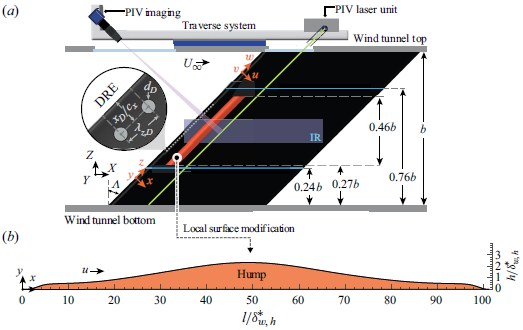
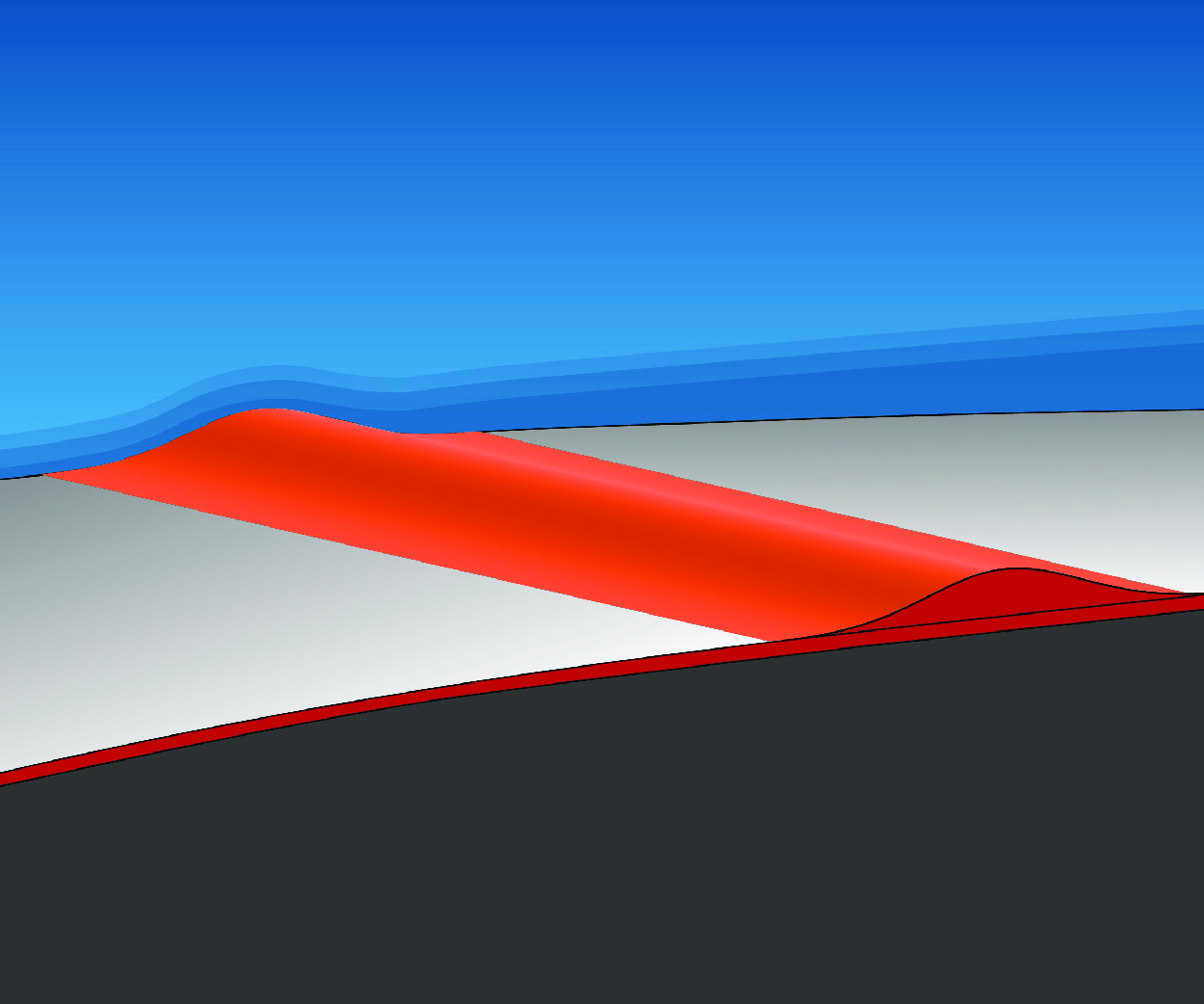
Figure 1. Experimental set-up: (a) Wing and measurement arrangement (flow direction from left to right). Surface hump (orange), the planar PIV set-up, infrared (IR) analysis region (blue shaded region, not to scale) and DRE details. (b) Measured cross-section geometry of the hump (vertical axis enlarged for visualisation, $\delta ^*_{w,h} = 485\, \unicode{x03BC} \text{m}$ ). Note the wing features a modified NACA 66 018 airfoil shape normal to the leading edge, for details see Serpieri (2018, pp. 28–29).

A common practice in the experimental study of CFI is the use of cylindrical discrete roughness elements (DRE) (see inset in figure 1 a) to confine the band of stationary CFI modes developing in the boundary layer (e.g. Downs & White 2013; Barth et al. 2018; Eppink 2020). Using linear parabolised stability equations (Haynes & Reed 2000) a spanwise wavelength of $\lambda _{z,D} \approx 7.5\,$ mm was identified as a part of the critical CFI modes (i.e. dangerous for transition), which feature a late-growth behaviour (Rius-Vidales & Kotsonis 2020) with respect to the hump location and reaches high amplification prior to natural transition at the conditions of this work. To trigger this critical mode, DRE with a nominal spanwise wavelength of $\lambda _{z,D} = 7.5\,$ mm, diameter of $d_D = 2\,$ mm and a height of $k_{D} = 25\,\unicode{x03BC} \text{m}$ were applied on the wing. It must be noted here, that while this forced critical mode represents a worst-case scenario for the reference case, the incoming CFI wavelength influence on the hump’s mechanisms is currently unknown, and can merit from dedicated future investigations.

The hump is manufactured as a surface add-on to the existing M3J model using negative CNC-fabricated moulds in which flexible epoxy resin compounds are cast. After curing, the resulting shape is verified using a Micro Epsilon LLT300025BL laser profilometer. Figure 1(b) shows the hump cross-sectional shape (i.e. orthogonal to the leading edge) obtained from laser measurement profiles averaged in the spanwise direction. The hump add-on is adhered to the surface of the wing parallel to the leading edge, with its apex centred at $x/c_x \approx 0.15$ as in figure 1(a). The hump geometry and M3J airfoil coordinates are available upon request to the authors. Note that the changes in geometry at the edges of the hump are necessary for the installation on the wing. The displacement thickness $\delta ^*_{w,h} = \int _0^{\delta _{99}}(1- ({\bar {w}_z}/{\bar {w}_e})) \textrm {d}y = 485\,\unicode{x03BC} \text{m}$ , based on the spanwise-averaged spanwise velocity profile ( $\bar {w}_z$ ), is measured at $x/c_x = 0.15$ for the reference (i.e. no hump) case and used for non-dimensionalisation of the hump geometry in figure 1(b).

The present work examines four test cases, namely A-C, A-H, B-C and B-H. Considering the same DRE arrangement (i.e. $k_D$ , $d_D$ and $\lambda _{z,D}$ , inset in figure 1 a), the resulting amplitude of CFI is effectively conditioned by the proximity of the DRE $(x_D/c_x)$ to the neutral point of the forced mode ( $x_{n}/c_x \approx$ 0.031). As such, the prefix A ( $x_{D}/c_x \approx$ 0.02) or B ( $x_{D}/c_x \approx$ 0.05) in the case ID specify the chordwise placement position of the DRE, and by consequence a high or low forced CFI amplitude, respectively. In addition, suffix C refers to the reference cases without hump while H refers to cases with a hump. Finally, it is important to note that in the presented results pertaining to cases A-H and B-H, the wall-normal coordinate $y$ is offset by the local height of the hump $h(x)$ . In addition, the displacement thickness $\delta ^*_{w,R} = 454\,\unicode{x03BC} \text{m}$ measured in the A-C case at $x/c_x = 0.13$ is used for non-dimensionalisation of the $y$ -coordinate.

2.2. Measurement techniques and data analysis

To identify the location of the laminar–turbulent transition, the surface temperature on the pressure side of the model is measured by an Optris PI640 IR camera (cropped sensor to $606$ pixel $\times$ $114$ pixel, spatial resolution of 0.6 pixels per mm and NETID 75 mK). The model’s surface is actively heated using halogen lamps placed on the exterior of the wind tunnel test section. Following Lemarechal et al. (2019) the temperature ratio between the model ( $T_m$ ) and the fluid ( $T_f$ ) was $T_m/T_f \leqslant 1.04$ (temperatures in degrees kelvin) to avoid thermal influence on transition. Thermal maps for each configuration described in § 2.1 are processed using an in-house MATLAB code to extract the transition location using a differential IR procedure described in Rius-Vidales & Kotsonis (2020). In this methodology a linear-fit on the identified transition front is performed along the span and extracted at mid-domain height (markers $\circ$ and $\diamond$ in figure 2 ai, aii,bi,bii). The confidence bands of this fit provide an indication of the uncertainty of the transition location across the span.

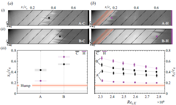
Figure 2. (ai,aii,bi,bii) Thermal maps (flow from left to right). Transition location ( $x_t$ ) (aiii) at $Re_{cX} = 2.3 \times 10^6$ and $\alpha = 3^\circ$ and (biii) for varying $Re_{cX}$ . Solid orange line and orange region indicate hump apex and width. Prefix A (high) and B (low) indicate the DRE forcing amplitude and solid grey lines their streamwise location. Suffix C indicates the reference case and H the hump case.

Planar two-dimensional, two-component particle image velocimetry (PIV) is used to characterise the CF vortices in the region of interaction with the hump. Measurements are conducted on $z$ – $y$ planes (i.e. parallel to the leading edge and quasinormal to the surface) at different chordwise positions between $0.1 \leqslant x/c_x \leqslant 0.4$ (figure 1 a). Images of the laser-illuminated and seeded flow are recorded using a LaVision Imager sCMOS camera ( $2560 \times 2160$ pixels, $6.5\,\unicode{x03BC} \text{m}$ pixel pitch, $f = 200\,\text{mm}$ , 2 $\times$ teleconverter). In total 1500 image pairs are acquired at sampling rate of 10 Hz per measurement plane. Final interrogation window of 12 $\times$ 12 pixel $^2$ and overlap of $75\,\%$ is reached. The uncertainty in the velocity mean value is estimated following the methodology presented by Sciacchitano & Wieneke (2016). For the measurements in this work the estimated maximum value of uncertainty is $U_{\bar {w}} = 0.36\, \% w_e$ and $U_{\bar {v}} = 0.27\, \% w_e$ . Following the methodology presented in Rius-Vidales & Kotsonis (2021), a spatial Fourier decomposition and reconstruction of the time-averaged results is applied to extract the primary CFI mode ( $m(0,1)$ ), its first higher harmonic ( $m(0,2)$ ) and a total perturbation field reconstructed as a truncated sum of the leading Fourier modes between the fundamental and the fourth higher harmonic (e.g. $\sum _n^5m(0,n)$ ) to reduce measurement noise (i.e. small spanwise wavelengths). Quantities extracted from these reconstructed flow fields are denoted with subscript $R$ .

Finally, as proposed by Downs & White (2013) the steady disturbance profile $\langle \hat {w}_R(y)\rangle _z$ at each PIV measurement plane ( $z$ - $y$ ) is calculated as $\langle \hat {w}_R(y)\rangle _z = \{({1}/{n})\sum _{j=1}^{n}[\bar {w}_R(y,z_j) - \bar {w}_{Rz}(y)]^2\}^{0.5}$ , where $j$ denotes a spanwise station index. Following the recommendations by Casacuberta et al. (2021, 2022) in cases of geometrical surface modifications, the maximum of the disturbance profile corresponding to the primary CFI is identified along the $y$ -coordinate at each chordwise position and its amplitude ( $A_T$ ) is retrieved to monitor chordwise changes of the CF vortices when interacting with the hump.

3. Results

3.1. Transition behaviour

Figure 2(ai,aii,bi,bii) shows the processed thermal maps corresponding to the four cases investigated in this work. A linear fit of the identified transition front along the wing’s span is applied and its projection to the mid-domain is indicated using the markers $\circ$ and  $\diamond$ . Note that the transition front is not exactly parallel to the leading edge due to the non-uniform wind tunnel blockage in the $Z$ -direction, which leads to a slightly stronger FPG on the wing’s outboard side. When comparing (figure 2 ai,aii, cases A-C to B-C), the dependence of the laminar–turbulent transition on the DRE forcing amplitude is observed. As expected, high-amplitude DRE forcing (condition A), results in the most upstream transition location. Note the sawtooth or jagged transition front, which previous studies have identified as a distinct feature of stationary CFI transition (e.g. Bippes 1999; Saric et al. 2003).

When the hump is present in each of the forcing cases A-H and B-H, a disparate transition behaviour occurs. At forcing condition A, the presence of the hump leads to a considerable reduction in the extent of laminar flow. In this case, the laminar–turbulent transition location is shifted upstream towards the hump location, as shown in figure 2(bi,aiii). In contrast, the presence of the hump at forcing condition B leads to a significant increase in the extent of laminar flow (figure 2 bii,aiii).

Figure 2(aiii) shows a transition delay (i.e. $\delta _t = x_{t,H}/c_x - x_{t,C }/c_x$ ) of approximately $14\,\%$ of the wing’s chord achieved in case B, maintaining laminar flow up to $x/c_x \approx 0.7$ . Pressure measurements for the reference case show that close to this location (i.e. $x/c_x \approx 0.65$ ), the wing undergoes a pressure changeover (i.e. favourable to adverse gradient) as the wing’s maximum thickness is reached. The rapid change to an adverse pressure gradient(APG) was previously observed to lead to the formation of a laminar separation bubble on this wing geometry (see Serpieri (2018); pp. 48–50). In addition, Wassermann & Kloker (2005) showed that the amplification of TS waves can occur in such pressure changeover regions. Therefore, it appears reasonable to assume that the transition delay effect of the hump in these experiments is artificially limited to approximately $\delta _t \approx 14\,\%$ of chord by forced transition not driven by CFI. This is further evidenced by the spanwise uniform and spatially smoothed transition front in case B-H, in contrast to the jagged and spatially sharp front in case B-C.

Given the transition delay behaviour that case B-H displays with respect to B-C, it becomes important to confirm the consistency of the effect at different conditions. Although not exhaustive, additional experiments with a variation in free stream Reynolds number ( $2.3 \times 10^6 \leqslant Re_{cX} \leqslant 2.8 \times 10^6$ ) are performed for both forcing conditions A and B. The results presented in figure 2(biii) show that the transition delay effect of the hump is robust to local changes in Reynolds number.

3.2. Boundary layer topology and development of primary CFI

This section investigates the novel transition delay by the surface hump by analysing the chordwise evolution of CF vortices, their spatial topology and the overall stability of the boundary layer for cases B-C and B-H (see § 2.1 for description of cases). For the remainder of this work, all results are presented for fixed conditions of $Re_{cX} = 2.3\times 10^6$ and $\alpha = 3^\circ$ . Figure 3(a–d) presents selected boundary layer profiles calculated as the spanwise velocity ( $\bar {w}_z$ ) averaged along the span (i.e. $z$ -coordinate) as extracted from each ( $z$ – $y$ ) PIV measurement plane (for orientation see figure 1 a). Note that these velocity profiles are representative of the spanwise-averaged mean flow and hence do not strictly correspond to the unperturbed base flow (e.g. laminar boundary layer solution in the absence of instabilities). In addition, due to the spanwise invariance of the swept-wing model, no significant pressure gradients occur along the $z$ -direction within the PIV domain. Therefore, due to momentum coupling in the conservation equations, any observed change in the spanwise velocity ( $w$ ) results from a direct change in the chordwise velocity ( $u$ , not measured in this work) by the hump.

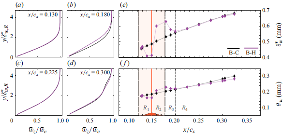
Figure 3. (a–d) Normalised mean and spanwise-averaged spanwise velocity ( $\bar {w}_z/\bar {w}_e$ ) profiles; (e) displacement thickness ( $\delta ^*_w$ ) and (f) momentum thickness ( $\theta _w$ ) for cases B-C (black) and B-H (magenta). Solid orange line indicates the hump apex location and shaded region its width.

For facilitating the discussion, the interaction of the hump with the incoming boundary layer flow is analysed considering four distinct spatial regions $R_{1}$ – $R_4$ as shown at the bottom of figure 3(f). The first region $R_1$ extends from the hump leading edge ( $x/c_x \approx$ 0.12) to its apex (i.e. hump’s crest) located at $x/c_x \approx 0.15$ . The time-averaged spanwise velocity profiles in figure 3(a) show that at $x/c_x \approx 0.13$ , the effect of the hump on the boundary layer flow is minimal. This is also reflected in the integral boundary layer quantities, namely displacement ( $\delta ^*_w$ ) and momentum thickness ( $\theta _w$ ) as shown in figure 3(e–f). Instead, by the downstream end of region $R_1$ , the influence of the hump on the boundary layer is noticeable and leads to a local flow acceleration and a reduction in $\delta ^*_w$ and $\theta _w$ . Through the direct coupling of the chordwise and spanwise momentum, a corresponding acceleration can be assumed for the $u$ velocity component, further suggesting the increase of the local pressure gradient (i.e. strengthening of the FPG) as shown in figure 3(e).

Downstream of the hump’s apex and until the downstream end of region $R_2$ at the trailing edge of the hump ( $x/c_x \approx$ 0.18), the curvature changes from convex to concave leads to a prolonged region of weakening of the local pressure gradient. This manifests as a deceleration of the boundary layer (figure 3 b) and an increase in $\delta ^*_w$ and $\theta _w$ as shown in figure 3(e–f). In contrast, in region $R_3$ , the nominal FPG of the wing leads to a local acceleration of the boundary layer and a recovery of $\delta ^*_w$ and $\theta _w$ towards reference case values starting from the hump’s trailing edge. Finally, considerably downstream of the hump apex (i.e. $x/c_x \approx 0.225$ , see figure 3 c) and within a fourth region $R_4$ , the boundary layer flow fully relaxes towards the reference case B-C. Even though minor differences exist in the integral boundary layer properties between cases B-C and B-H in region $R_4$ (see figure 3 e–f), the boundary layer profile for the B-C case without hump at $x/c_x \approx 0.3$ shows a stronger spanwise distortion of the boundary layer flow than the case B-H with the hump (see figure 3 d).

Figure 4 presents the time-averaged spanwise boundary layer velocity ( $\bar w_R$ ) measured in the $z$ – $y$ plane at the chordwise stations matching the selected profiles in figure 3(a–d). Note the $z^*$ -coordinate is shifted with respect to the $z$ -coordinate origin such that the CF vortices align between presented chordwise stations. For case B-C (figure 4 ai –di), the imprint of the corotating CF vortices on the boundary layer flow is evident. Analysing the most downstream station ( $x/c_x = 0.300$ in figure 4 di) reveals two regions of interest in the structure of the stationary CF vortices, namely, the upwelling ( $\ominus$ in figure 4 di) region where low momentum flow is transferred away from the wall and the downwelling region ( $\oplus$ in figure 4 di) where high momentum flow is transferred towards the wall.

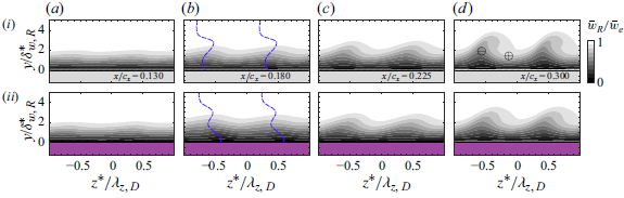
Figure 4. Contours of normalised mean spanwise velocity ( $\bar {w}_R/\bar {w}_e$ ) for cases (i) B-C and (ii) B-H. Dashed blue constant phase isolines for $m(0,1)$ . All fields are spatially filtered (i.e. $\sum _n^5m(0,n)$ ).

The modifications of the topology of the boundary layer flow in figure 4 reveal essential features for the discussion that follows: (i) upstream of the hump apex in region $R_1$ (figure 4 ai,aii), there is no discernible change in the topology between cases; (ii) downstream of the hump’s apex in region $R_2$ (figure 4 bi, bii), the distortion on the mean flow differs between cases. As shown by lines of constant phase (see blue dashed lines in figure 4 bi,bii), the reference case B-C (figure 4 bi) shows a tilting of the perturbation system in the direction of the $z^*$ positive axis, i.e. matching the expected nominal clockwise rotation of the CF vortices in the FPG region. Instead, in the case B-H with hump (figure 4 bii), tilting of the perturbation occurs in the opposite direction (i.e. towards the negative $z^*$ axis) and resembles the flow topology presented by Wassermann & Kloker (2005; figure 8a) when studying the effect of a pressure change-over (i.e. favourable to adverse gradient) on CFI; (iii) although in regions $R_3$ and $R_4$ downstream of the hump (figure 4 ci,cii) the orientation and topology of the CF vortices recover to the one of the reference case B-C, the stability of the CF vortices in case B-H has been fundamentally altered by the interaction with the hump, since the mean flow spanwise modulation is noticeably weaker than the reference case B-C by the end of the measurement domain (compare figure 4 di,dii).

To evaluate the effect of the hump on the stability of the incoming CF vortices, figure 5(a–d) presents selected disturbance profiles $\langle \hat {w}_R\rangle _z$ calculated following the methodology described in § 2.2. At the most upstream location in region $R_1$ ( $x/c_x \approx 0.13$ , figure 5 a), the shape of this profile (i.e. only one lobe) indicates a weak spanwise distortion typical of the linear CFI amplification regime. Downstream of the hump apex in region $R_2$ ( $x/c_x \approx 0.18$ , figure 5 b), a second lobe appears near the wall ( $y/\delta ^*_{w,R} \approx 1$ ). Although the experimental set-up does not allow for the direct measurement of pressure distribution in the hump case, one can infer from the changes in $\delta ^*_w$ and $\theta _w$ (figure 3 e–f) that an APG region develops downstream of the hump apex ( $0.16 \lesssim x/c_x \lesssim 0.18$ ) followed by the recovery to the nominal FPG of the wing. These changes in pressure gradient correlate with the respective local decrease in region $R_2$ and increase in region $R_3$ of the amplitude $A_T$ in figure 5(e) calculated from reconstructed flow fields using the Fourier modes between the primary and the fourth higher harmonic (i.e. total perturbation $\sum _n^5 m(0,n)$ , solid line), the primary mode $m(0,1)$ (dashed line) and its first higher-order harmonic $m(0,2)$ (dash–dotted line) as described in § 2.2. More importantly, farther downstream in region $R_4$ , a significant local stabilisation effect on the primary CFI mode $m(0,1)$ and its first higher-order harmonic $m(0,2)$ occurs.

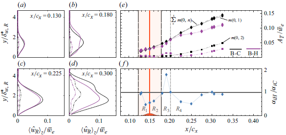
Figure 5. (a–d) Steady disturbance $\langle \hat {w}_R\rangle _z$ profile shape $m(0,1)$ (solid line) and $m(0,2)$ (dash–dotted line) for B-C (black) and B-H (magenta); (e) chordwise evolution of amplitude $A_T$ and (f) ratio of growth rates $\alpha _{iH}/\alpha _{iC}$ for cases B-C and B-H. Solid orange line indicates the hump apex location and shaded region its width.

The stabilisation of the fundamental and first higher-order harmonic CFI modes well within $R_4$ ( $x\geqslant 0.25$ ) is a rather unexpected observation, inasmuch as figure 3(e) shows a full recovery of the boundary layer flow to the reference case by $x/c_x \approx 0.2$ . Nonetheless, the interaction of the incoming flow with the hump alters significantly the stability of the primary CFI mode $m(0,1)$ as evidenced by the relative change in its growth rate shown in figure 5(f). Note, the relative change is calculated as the ratio ( $\alpha _{iH}/\alpha _{iC}$ ) where $\alpha _{iH,iC} = -({1}/{A_T})({\partial {A_T}}/{\partial {x}})|_{H,C}$ .

3.3. Primary CFI stabilisation mechanism by the hump

This section investigates the chordwise evolution of the primary CFI perturbation near the hump. The spanwise perturbation velocity $\hat w$ is evaluated as $\hat w = \bar w - \bar w_z$ . Figure 6 shows contours of the spanwise perturbation velocity field for the primary CFI mode $\hat w_{R(0,1)}$ and its first higher harmonic $\hat w_{R(0,2)}$ . In the reference case, the primary mode manifests as regions of negative and positive spanwise velocity. As expected, due to the wing’s nominal FPG, the CF vortices rotate clockwise when viewed from downstream (i.e. looking towards the $-x$ direction) and tilt the perturbation field towards the $z^*$ -coordinate positive direction. Figure 6(v) demonstrates lines of constant perturbation phase obtained by tracking the local minimum of perturbation velocity of the primary CFI $m(0,1)$ . For the reference case B-C in figure 6(v), only a slight change in the orientation of the perturbation is observed in the measurement region. Instead, the hump case B-H shows that in region $R_3$ ( $x/c_x = 0.180$ ), the orientation (i.e. spanwise phase) of the primary mode disturbance $\hat w_{R(0,1)}$ (figure 6 aii) is significantly altered compared with the one dictated by the reference case B-C (figure 6 ai). Only considerably downstream of the hump at region $R_4$ (i.e. $x/c_x \gt 0.2$ ) the perturbation shape of case B-H realigns with the one of B-C. Analysing figure 6(iii–iv) reveal that the first higher harmonic $m(0,2)$ also follows similar topological changes and stabilisation by the end of the measurement region as shown in figure 5(e).

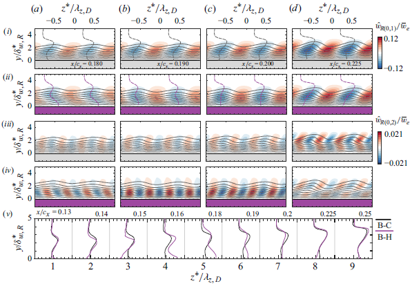
Figure 6. Contours of steady spanwise perturbation for (i,ii) primary CFI mode $m(0,1)$ and its first (iii,iv) higher harmonic $m(0,2)$ for case (i,iii) B-C and (ii,iv) B-H. Grey solid lines correspond to $\bar w_R$ contour levels in figure 4, dashed lines corresponds to constant phase isolines for $m(0,1)$ . (v) Constant phase isolines of the primary CFI mode $m(0,1)$ . For visualisation purpose the constant phase isolines spanwise coordinate ( $z^*/\lambda _{z,D}$ ) is shifted by 1 between presented chordwise locations in (v).

Although the exact cause of this orientation change in the perturbation topology cannot be adequately identified with the available measurements, the good qualitative comparison with the topology presented by Wassermann & Kloker (2005; figure 8b) suggests a connection to a possible weakening or reversal of the CF velocity component near the wall over region $R_2$ . The combination of observations stemming from the reported measurements provides a first handle towards elucidating the stabilisation mechanism activated by the presence of the hump. This can be summarised as follows: the hump surface modification leads to a local pressure gradient modification which manifests in successive acceleration and deceleration events in the chordwise ( $u$ ) and spanwise ( $w$ ) velocity components as the flow convects over the hump (see figure 3 e–f). These local changes in the boundary layer potentially lead to a region of CF velocity weakening or even reversal downstream of the hump apex which distorts the organisation of the primary CFI mode. This distortion is exemplified through a notable spatial tilting of the perturbation structures in the opposite direction of their nominal orientation (see figure 6 v). The stability characteristics of the distorted primary instability can be expected to be significantly altered due to this distortion, as the perturbation shape function no longer corresponds to a classic ‘modal’ CFI. This is also evident in the measured growth rate, which is found to decrease with respect to the reference case, leading to a less optimal growth downstream of the hump, even though the boundary layer has fully recovered to the baseline conditions (see figure 5 e–f). Expectedly, the reduced growth in the perturbation system leads to a delay of laminar–turbulent transition.

Overall, the observed CFI stabilisation behaviour by the hump merits detailed numerical investigations to characterise the reversal of the CF velocity component. In addition, an assessment of flow non-parallelism and possible non-modal growth/decay effects is important in light of the ‘reverse lift-up effect’ recently proposed by Casacuberta et al. (2024) as a possible stabilisation mechanism of CFI by forward-facing steps.

3.4. Development of secondary CFI and laminar breakdown

Past investigations of CFI in nominally smooth geometries have shown that the breakdown of the stationary CF vortices occurs through the rapid development of secondary unsteady CFI modes. These modes are known as type I, II and III (see Malik et al. 1996; Wassermann & Kloker 2002, 2003), depending on their spatial topology as well as their frequency content. As such, a holistic study of the development of secondary instabilities and the following laminar breakdown of the stationary CF vortices requires a frequency analysis and spectral filtering of unsteady velocity measurements. Such analysis is beyond this work’s scope due to the PIV measurements’ low repetition rate of 10 Hz. Nonetheless, valuable information on the development of secondary CFI modes and their role on the hump-derived transition delay can be inferred from the spatial distribution and streamwise evolution of time-averaged spanwise velocity gradients ( $\partial \bar {w}_R /\partial z$ and $\partial \bar {w}_R /\partial y$ ) presented in figure 7 and the standard deviation of temporal velocity fluctuations ( $\sigma _{w_R}$ ) presented in figure 8.

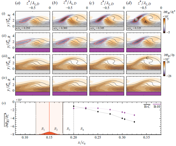
Figure 7. Contours of spanwise (i,ii) and wall-normal (iii,iv) gradients of spanwise velocity for cases (i,iii) B-C and (ii,iv) B-H. Grey solid lines correspond to the $\bar {w}_R$ contour levels in figure 4. (v) Streamwise evolution of average spanwise gradients inside the regions delimited by orange dashed lines in contours. All fields are spatially filtered (i.e. $\sum _n^5m(0,n)$ ).

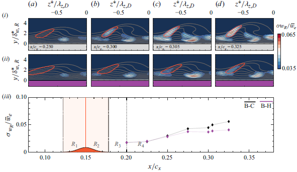
Figure 8. Contours of standard deviation of temporal spanwise velocity fluctuations ( $\sigma _{w_R}/\bar {w_R}$ ) for cases (i) B-C and (ii) B-H. Grey solid lines correspond to the $\bar {w}_R$ contour levels in figure 4. (iii) Streamwise evolution of the maximum standard deviation of temporal velocity fluctuations inside the regions delimited by orange dashed lines. All fields are spatially filtered (i.e. $\sum _n^5m(0,n)$ ).

The type III mode is related to the interaction between travelling and stationary CFI modes, and can be in fact classified as a nonlinear interaction of primary instabilities. These manifest as low-frequency velocity fluctuations on the inner side of the upwelling region (regions of $\partial \bar {w}_R /\partial z \gt 0$ , A in figure 7 di). In contrast, type I and II modes have been associated with Kelvin–Helmholtz type shear layer instabilities and manifest as high-frequency velocity fluctuations on the outer side (regions of $\partial \bar {w}_R /\partial z \lt 0$ , B in figure 7 di) and the top of the stationary CF vortices (regions of $\partial \bar {w}_R /\partial y \gt 0$ , C in figure 7 diii). Depending on the relative dominance of external factors, such as surface roughness and free stream turbulence, laminar breakdown in swept-wing geometries is eventually driven by one or more of the aforementioned types of secondary CFI (Bippes 1999). Specifically at conditions of low free stream turbulence, pertinent to the present work, transition is found to ensue through the explosive amplification of type I modes (Serpieri & Kotsonis 2016).

Figure 7(ai–di,aiii–diii) examines the time-averaged spanwise and wall-normal shears in selected $y$ – $z$ planes. Such examination is motivated by the well-established role of stationary shear on the development and growth of secondary CFI modes (Malik et al. 1996). In the reference case B-C, measurements reveal a gradual streamwise increase in the spanwise and wall-normal shears on the inner ( $\partial \bar {w}_R /\partial z \gt 0$ ), outer ( $\partial \bar {w}_R /\partial z \lt 0$ ) and top side of the upwelling region. When comparing with the hump case B-H in figure 7(bii–dii,biv–div), an overall and notable reduction of intensity of spanwise gradients ( $\partial \bar {w}_R /\partial z$ ) on the outer and inner side of the CF vortices is observed. Wall-normal gradients ( $\partial \bar {w}_R /\partial y$ ) show a relatively more moderate change compared with their spanwise counterparts, albeit still reduced due to the hump.

The following analysis primarily focuses on the negative spanwise shears (region B in figure 7 di) as, in the present conditions and facility, laminar breakdown was found to mainly ensue through the type I secondary mode, directly linked to the spanwise flow shears (Serpieri & Kotsonis 2016). To further quantify the pertinent changes of spanwise flow shear due to the hump, a statistical average is extracted within areas of elevated shears. The boundaries of the extraction regions are therefore determined at each measurement plane as isolines of 60 % of the minimum $\partial \bar {w}_R /\partial z$ and delimited in figure 7(ai–di,aii–dii) by the orange dashed lines. The spatially averaged spanwise shears within these extraction regions are shown in figure 7(v). The results further highlight an overall reduction of the spanwise flow gradients due to the hump. This is a direct consequence of the weakening of the primary CFI amplitude due to the hump, as described in § 3.3.

Following the relation of type I secondary CFI and spanwise shears, an examination of the unsteady velocity fluctuations within the topology of the stationary CFI can provide insight into the development of secondary CFI modes and their response to the hump effect. Figure 8(ai–di,aii–dii) presents the spatial distribution of the standard deviation of temporal velocity fluctuations at selected $y$ – $z$ planes, for the reference and hump cases. Distinct areas of elevated velocity fluctuations are evident, closely following the well-established spatial distribution of fluctuating content of secondary CFI development as identified in past experimental and numerical works (e.g. Malik et al. 1996; White & Saric 2005). As noted, frequency-based segregation of these structures is presently unattainable due to the limited temporal resolution of the current PIV measurements. However, the spatial arrangement of elevated fluctuations can be used as proxy to their spatiotemporal nature. Specifically, an area of notable fluctuations is found to directly overlap with earlier identified regions of elevated negative spanwise shears, delimited by orange dashed lines in figures 7(ai–di,aii–dii) and 8(ai–di,aii–dii). To further quantify the relative intensity of velocity fluctuations between reference and hump case, figure 8(iii) presents the maximum value of temporal spanwise velocity fluctuations ( $\sigma _{w_R}$ ) found inside the regions delimited by the orange dashed lines, for the reference case B-C (figure 8 ai–di) and hump case B-H (figure 8 aii– dii). A notable reduction of the intensity of the temporal velocity fluctuations ( $\sigma _{w_R}$ ) is found when the hump is present, in the region overlapping with $\partial \bar {w}_R /\partial z \lt 0$ where type I secondary CFI modes typically develop (e.g. White & Saric 2005; Serpieri & Kotsonis 2016).

Serpieri & Kotsonis (2016) show that under similar reference conditions (i.e. model and wind tunnel) type I secondary CFI modes are the driving mechanism for laminar–turbulent transition. Eventually, the combination of observations presented in §§ 3.3 and 3.4 provide a closure to the overall transition delay mechanism enabled by the hump. Specifically, the ensuing stabilisation and amplitude suppression of the primary CFI as described in § 3.3 leads to a corresponding weakening of pertinent spanwise shears in the flow (figure 7). These shears are known to support the development of unsteady type I secondary CFI modes and thus by association, these are also found weakened due to the hump. The weakening of type I secondary CFI can be directly linked to the downstream postponement of laminar breakdown, as established through IR imaging in § 3.1.

4. Concluding remarks

The demonstrated potential of spanwise-invariant surface features (i.e. Ivanov & Mischenko 2019; Rius-Vidales & Kotsonis 2021) to delay swept-wing transition motivated the authors to propose and assess experimentally a shallow smooth surface modification in the form of a hump, as a passive LFC device. The analysis of the transition behaviour using thermal surface maps reveals that the amplitude with which the primary CFI reaches the hump plays a significant role in determining their interaction dynamics. For a high primary CFI amplitude, the addition of the hump leads to a transition advancement. In contrast, at a lower primary CFI amplitude, the hump leads to a novel and considerable transition delay which appears to be robust to moderate changes in chord Reynolds number.

Detailed measurement of the development and interaction of the lower-amplitude primary CFI with the hump reveals four regions of interest. In the first region, which extends from the hump leading edge to its apex (i.e. the hump’s crest), the hump geometry imposes a local FPG on the boundary layer. This decrease in pressure leads to a momentum gain and a slight amplification of the primary CFI. Downstream of the hump apex and into the second and third region, the APG imposed by the hump geometry leads to a prolonged loss of momentum in the boundary layer, a slight decrease in the amplitude of the primary CFI, and a considerable change in their wall-normal orientation (i.e. tilting). Although the exact origin of the primary CFI spatial orientation change is still elusive, the good qualitative comparison with the topology presented by Wassermann & Kloker (2005; figure 8b) points to a possible connection with CF reversal. Finally, in the fourth region, a considerable stabilisation of the primary CFI occurs, indicating that the interaction with the hump in the previous regions has fundamentally altered its stability characteristics.

As a consequence of the stabilisation of the primary CFI by the hump, an overall reduction in spanwise velocity gradients and a decrease in the intensity of the temporal velocity fluctuations on the outer side of the upwelling region is observed. The spatial location and topology of the temporal velocity fluctuations points to the postponement of the onset of unsteady secondary CFI modes of type I to a more downstream position, offering in this way an explanation to the observed transition delay by the hump.

Overall, this work provides the first experimental evidence that under certain conditions a smooth surface hump stabilises the primary CFI instability resulting in a considerable transition delay. The effective manipulation of transition by the hump makes it a viable candidate device for passive flow control in future laminar flow wings.