Drawing of weakly viscoelastic fluid tubes

Abstract

We explore the drawing of an axisymmetric viscoelastic tube subject to inertial and surface tension effects. We adopt the Giesekus constitutive model and derive asymptotic long-wave equations for weakly viscoelastic effects. Intuitively, one might imagine that the elastic stresses should act to prevent hole closure during the drawing process. Surprisingly, our results show that the hole closure at the take-up point is enhanced by elastic effects for most parameter values. However, the opposite is true if the tube has a sufficiently large hole size at the inlet nozzle of the device or if the axial stretching is sufficiently weak. We explain the physical mechanism underlying this phenomenon by examining how the second normal stress difference induced by elastic effects modifies the hole evolution process. We also determine how viscoelasticity affects the stability of the drawing process and show that elastic effects are always destabilising for negligible inertia. On the other hand, our results show that if the inertia is non-zero, elastic effects can be either stabilising or destabilising depending on the parameters.

1. Introduction

Optical fibres form a critical component of the modern interconnected world in which information must be transmitted over extremely long distances and at high speeds in a secure and reliable way. In recent years the use of microstructured optical fibres (MOFs) has become significant in a number of applications (Pal 2010; Chen et al. 2016; Liu et al. 2017). Such MOFs are fibres that contain an array of air holes that run parallel to the axis of the fibre. The air holes modify the optical transmission properties and allow for fibres with highly customisable optical properties that are extremely valuable in a number of important applications. These include micro-electrode fabrication (Puil et al. 2003; Huang et al. 2007), microscopy fabrication (Gallacchi et al. 2001) and high-accuracy sensing (Xue et al. 2023). The optical properties are highly sensitive to small deviations in the hole geometry, and it is therefore extremely important to have a very carefully controlled fabrication process.

The most common method for fabricating fibres is by taking a relatively large preform with a hole structure and stretching it so as to reduce the cross-sectional area by factors of up to 10 000 times. For Newtonian materials, in the absence of surface tension, theoretical results have shown that the stretching process will precisely reduce the relative size of the thread whilst maintaining the geometry (Dewynne, Howell & Wilmott 1994). However, in real-world applications surface tension effects are non-negligible and this can cause significant deviations in the shapes and positions of the hole structures. This is particularly critical in the production of MOFs, as the optical properties are highly sensitive to the hole geometry. In some cases, some of the holes may even close. Pressurising air channels can be used to prevent this but also causes geometry changes and may cause holes to burst (Chen et al. 2016). Therefore, one needs to take into account the effects of surface tension and pressure to ensure that the desired hole structure is achieved in the extended fibre. Another important issue in the fabrication process is that the drawing of threads is subject to an oscillatory instability, known as draw resonance, which causes non-uniformities in the axial thread profiles (Denn 1980). If severe, this will render an optical fibre not fit for purpose. Suppressing instabilities of this type is therefore a critical aspect of fibre fabrication.

In the case of MOFs, Chen et al. (2015, 2016) showed that surface tension can dramatically affect the sizes and shapes of the holes and their experiments demonstrated that the hole dynamics can be extremely difficult to control. Their experiments were performed using glass materials that are well approximated as being Newtonian. In fact, most MOFs are made from glass materials, but there has been growing interest in using polymer materials for fibre production. Early experiments using polymeric materials were conducted by Demay & Agassant (1985) who investigated the draw resonance phenomenon for fibres without holes under nearly isothermal conditions using four different polyesters. The experimental findings are in accordance with non-isothermal and viscoelastic computations and demonstrated that an increase in viscoelastic properties leads to enhanced stability. More recently there have been numerous experimental studies that examined various characteristics of drawing using polymeric materials (Van Eijkelenborg et al. 2001; Large et al. 2008; Argyros 2013; Gierej et al. 2022). Polymer fibres offer advantages such as lower processing temperatures and ease of preform creation, and a wide range of polymers have been found suitable for the fabrication process. Unlike glass materials, polymer materials can exhibit significant viscoelasticity. This leads to the question of whether viscoelastic polymeric materials can be utilised to better achieve the manufacturing goals of preserving internal hole structures and controlling instabilities. Hence, a motivation of this work is to determine how elastic effects can be leveraged to improve the fabrication process for the drawing of ‘holey’ fibres and other related applications.

The drawing of threads has an extensive history dating back to Matovich & Pearson (1969) who considered the drawing of a Newtonian solid thread (with no holes) and determined the criteria for instability. Shah & Pearson (1972) proposed a generalised theoretical model by considering the effects of inertia, gravity and surface tension, along with thermal effects. It turns out that the interaction between the various physical effects gives rise to complicated and very rich dynamics that has been studied by a number of authors (Geyling 1976; Geyling & Homsy 1980; Cummings & Howell 1999; Forest & Zhou 2001; Wylie, Huang & Miura 2007; Suman & Kumar 2009; Taroni et al. 2013; Bechert & Scheid 2017; Philippi et al. 2022). All of these works considered Newtonian solid threads with no internal holes.

The dynamics of drawing solid threads composed of viscoelastic fluids has also been widely investigated. Denn, Petrie & Avenas (1975) neglected surface tension and inertia, proposed approximate equations and obtained the steady-state solutions for a thread composed of a generalised Maxwell material. Fisher & Denn (1976) extended the study by including the deformation-rate dependency of polymeric materials (White–Metzner model) and performed a linear stability analysis. Jung & Hyun (1999) developed a simple approximate method for determining the stability threshold for a viscoelastic solid thread, and the mechanism for draw resonance was discussed by Hyun et al. (1999). Park (1990) considered the steady drawing process of a two-phase compound fibre, in which the core is a Newtonian fluid surrounded by a sheath layer that is modelled as a weakly upper-convected Maxwell fluid. Lee & Park (1995) studied the stability of this type of flow. Gupta & Chokshi (2017) considered the linear stability of a compound fibre whose core is described using the extended pom-pom (XPP) model and whose sheath layer is described using the upper-convected Maxwell model. Under non-isothermal drawing, Zhou & Kumar (2010) investigated the steady state and linear stability of the non-isothermal drawing of viscoelastic fibres whose viscosity varies with temperature. Zhou et al. (2011) examined the melt-blowing process of viscoelastic materials modelled under varying temperature conditions, performing linear stability and sensitivity analyses. Gupta & Chokshi (2018) considered the stability of the drawing of a polymeric fluid described by the XPP model in the presence of thermal effects. Nevertheless, they argued that, for small-air-gap flows the role of thermal effects in stability is negligible (Demay & Agassant 1985; Gupta & Chokshi 2015). In fact, there are many works considering various aspects of the drawing of viscoelastic threads: Van der Walt et al. (2012) considered generalised boundary conditions and Gupta & Chokshi (2015) performed a weakly nonlinear analysis. All of these studies involved fluid flows with no internal holes.

Early work on the drawing of Newtonian threads with holes was performed by Pearson & Petrie (1970a , b ). Subsequently, Fitt et al. (2001, 2002) derived an asymptotic mathematical model for the drawing of axisymmetric threads with an internal hole. They showed that there are negligible leading-order pressure gradients in the radial direction and so similar mathematical techniques to those used in the case of a solid thread could be used. Griffiths & Howell (2007, 2008) and Stokes et al. (2014) developed a general mathematical framework for analysing non-axisymmetric threads. This was generalised to include internal pressurisation of holes (Chen et al. 2015) and thermal effects (Stokes, Wylie & Chen 2019). To our best knowledge, there are very few studies that consider the draw resonance instability of threads with internal hole structure. Only very recently, Wylie et al. (2023) studied the draw resonance instability of MOFs with internal holes. All of these works are for Newtonian fluids.

Despite the extensive work on the drawing of Newtonian threads with holes, there has been no systematic derivation or examination of viscoelastic threads with holes. At first sight, this seems to be perplexing until one realises that in the case of viscoelastic threads there are capillary forces acting on the inside of the holes that induce pressure gradients in the radial direction that are not present in the Newtonian case. These radial pressure gradients introduce complicated feedback mechanisms between the axial and perpendicular flows that fundamentally modify the rate at which holes close and the stability characteristics of the flow. In fact, we will show that these radial pressure gradients are crucial to understanding the role that viscoelasticity plays. From a technical viewpoint the radial pressure gradients prevent one from applying the techniques used by previous authors such as Fitt et al. (2001) and Stokes et al. (2019). Nevertheless, we adopt the Giesekus constitutive model (Giesekus 1982) and derive asymptotic long-wave equations that allow us to determine how weakly viscoelastic effects modify the Newtonian flow. Elastic effects are known to hinder the surface-tension-driven pinching that occurs in threads without holes (Entov & Hinch 1997; Li & Fontelos 2003). Therefore, it seems reasonable that elastic stresses should oppose any inward radial flow generated by surface tension and hence act to reduce hole closure during the drawing process. However, surprisingly, we show that elasticity typically tends to induce more rapid hole closure. On the other hand, the opposite is true if the tube has a sufficiently thin wall at the inlet nozzle of the device or if the axial stretching is sufficiently weak. By carefully examining the expressions for the hole size at the take-up point we explain how the second normal stress difference induced by elastic effects modifies the hole evolution process. Furthermore, we consider the draw resonance instability and determine whether elastic effects stabilise or destabilise the drawing process. We show that if inertia is negligible then elastic effects always act to destabilise the flow. However, for non-zero inertia, elastic effects can be either stabilising or destabilising depending on the surface tension, inlet hole size and parameters that describe the constitutive behaviour.

The paper is structured as follows. Section 2 presents the model formulation and derives the governing equations using the assumption of a slender tube. Section 3 explores the weakly elastic limit and derives the long-wave nonlinear system that describes the drawing of an axisymmetric tube made of a viscoelastic fluid. Section 4 discusses the steady-state profiles and explains how elasticity influences hole evolution. Section 5 conducts a linear stability analysis to assess the impact of elasticity on the stability of the drawing process. Finally, § 6 provides a discussion of the results.

2. Model formulation

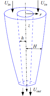
Figure 1. Schematic of the drawing process for a viscoelastic tube.

We consider a slender axisymmetric tube composed of a viscoelastic incompressible fluid. This fluid is fed through a nozzle of a drawing device with a constant velocity $U_{in}$ . At the nozzle the outer radius is denoted by $H_{in}$ , and the inner one by $h_{in}$ . We define $\phi =h_{in}/H_{in}$ to be the ratio of the inner to the outer radius at the input nozzle with $0\lt \phi \lt 1$ . At a distance $L$ from the nozzle, the tube is pulled by a take-up roller such that the tube has a speed $U_{out}$ . Our focus in the present work is the flow from the inlet nozzle ( $z=0$ ) to the take-up point ( $z=L$ ). For simplicity we do not consider pressurisation of the air channel, although it is straightforward to generalise. In what follows, $z$ is the distance measured along the axis of the tube, $r$ is the distance measured radially outward from the axis of the tube, $\theta$ is the azimuthal coordinate and $t$ is the time. The inner and outer radii of the tube are denoted by $h(z, t)$ and $H(z,t)$ , respectively, as shown in figure 1. The fluid has a velocity field $\textbf{u}=(v, 0, u)$ in cylindrical coordinates, where $v,\ 0$ and $u$ are the velocity components in the $r,\ \theta$ and $z$ directions, respectively.

The equations for the fluid tube are given by conservation of mass and momentum:

(2.1) \begin{align} &\boldsymbol{\nabla }\cdot \textbf{u}=0, \end{align}

(2.2) \begin{align} &\rho (\textbf{u}_{,t}+\textbf{u}\cdot \boldsymbol{\nabla }\textbf{u})=\boldsymbol{\nabla }\cdot \boldsymbol{\sigma }, \end{align}

where a comma is used to represent partial derivative with respect to the letter following the comma, $\boldsymbol{\nabla }$ is the differential operator given by $\boldsymbol{\nabla }=(\partial _r, \partial _\theta /r, \partial _z)$ in cylindrical coordinates, $\rho$ is the density and $\boldsymbol{\sigma }$ is the total stress tensor. We assume that the viscoelasticity in the fluid arises from polymers that are dissolved in a Newtonian solvent and adopt the Giesekus model (Giesekus 1982). Therefore, the stress tensor $\boldsymbol{\sigma }$ satisfies the following constitutive relation:

(2.3) \begin{align} &\boldsymbol{\sigma }=-p\textbf{I}+2\eta _s\textbf{D}+\boldsymbol{\tau }, \end{align}

(2.4) \begin{align} &\boldsymbol{\tau }+\lambda \overset {\triangledown }{\boldsymbol{\tau }}+\frac {\alpha \lambda }{\eta _p}(\boldsymbol{\tau })^2=2\eta _p\textbf{D}, \end{align}

(2.5) \begin{align} &\overset {\triangledown }{\boldsymbol{\tau }}=\boldsymbol{\tau }_{,t}+\textbf{u}\cdot \boldsymbol{\nabla }\boldsymbol{\tau }-(\boldsymbol{\nabla }\textbf{u})^\intercal \cdot \boldsymbol{\tau }-\boldsymbol{\tau }\cdot (\boldsymbol{\nabla }\textbf{u}), \end{align}

where $p$ is the pressure, $\textbf{I}$ is the identity matrix, $\textbf{D}=(\boldsymbol{\nabla }\textbf{u}+(\boldsymbol{\nabla }\textbf{u})^\intercal)/2$ is the strain-rate tensor, $\eta _s$ is the viscosity of the solvent, $\eta _p$ is the viscosity of the polymer, $\boldsymbol{\tau }$ is the polymer stress tensor and $\lambda$ is the relaxation time for the polymer. The parameter $\alpha$ is the mobility factor which is dimensionless and represents the importance of the quadratic term in the constitutive law (2.4). In the case of $\alpha =0$ , the Giesekus model reduces to the Oldroyd-B model (Oldroyd 1950). For $\alpha =0$ and $\eta _s=0$ , the Giesekus model reduces to the upper-convected Maxwell model. One well-known drawback of the Oldroyd-B and upper-convected Maxwell models is that they can give rise to infinite stresses at finite elongational rates (Bird, Armstrong & Hassager 1987; Renardy 2000; Tanner 2000; Evans, Palhares Junior & Oishi 2017). The Giesekus model removes this unphysical feature by adding a term that is quadratic in the stress tensor into the constitutive relation. We note that $\alpha$ should be smaller than $0.5$ to avoid a non-monotonic dependence of the shear stress on the shear rate in simple shear flows (Morozov & Spagnolie 2015). In the weakly viscoelastic regime, where the relaxation time is much shorter than the characteristic time of the flow, the Giesekus model simplifies to a type of second-order fluid model. This is achieved by expanding the polymer stress tensor in a series based on the relaxation time. In addition, for simple steady shear flow, the shear viscosity in the Giesekus model remains bounded for finite shear rates. For the simple steady extensional flow, the extensional viscosity and normal stress differences of the Giesekus model are also bounded for any finite extension rate. For further details, we refer the reader to Giesekus (1982), Barrow et al. (2004) and Minh (2023).

On the inner and outer surfaces of the tube, the dynamic boundary conditions are

(2.6) \begin{align} &\textbf{n}_1\cdot \boldsymbol{\sigma }\cdot \textbf{n}_1=-\gamma \kappa _1,\quad \textbf{t}_1\cdot \boldsymbol{\sigma }\cdot \textbf{n}_1=0\quad \text{at}\quad r=h(z,t), \end{align}

(2.7) \begin{align} &\textbf{n}_2\cdot \boldsymbol{\sigma }\cdot \textbf{n}_2=-\gamma \kappa _2,\quad \textbf{t}_2\cdot \boldsymbol{\sigma }\cdot \textbf{n}_2=0\quad \text{at}\quad r=H(z,t). \end{align}

Here, $\gamma$ is the surface tension and $\kappa _1{\kern-1pt}$ and $\kappa _2$ are the mean curvatures of inner and outer surfaces, respectively, given by

(2.8) \begin{align} \kappa _1=\left [\frac {h_{,zz}}{(1+h_{,z}^2)^{3/2}}-\frac {1}{h(1+h_{,z}^2)^{1/2}}\right],\quad \kappa _2=-\left [\frac {H_{,zz}}{(1+H_{,z}^2)^{3/2}}-\frac {1}{H(1+H_{,z}^2)^{1/2}}\right]. \end{align}

The vectors $\textbf{n}_i$ and $\textbf{t}_{i}$ $(i=1,\ 2)$ are the unit vectors on the inner and outer surfaces in the normal and tangential directions, which are given by

(2.9) \begin{align} &\textbf{n}_1=\frac {1}{\sqrt {1+h_{,z}^2}}(-1,\ 0,\ h_{,z}),\quad \textbf{n}_2=\frac {-1}{\sqrt {1+H_{,z}^2}}(-1,\ 0,\ H_{,z}), \end{align}

(2.10) \begin{align} &\textbf{t}_1=\frac {1}{\sqrt {1+h_{,z}^2}}(h_{,z},\ 0,\ 1),\quad \textbf{t}_2=\frac {-1}{\sqrt {1+H_{,z}^2}}(H_{,z},\ 0,\ 1). \end{align}

The kinematic boundary conditions are

(2.11) \begin{align} h_{,t}+uh_{,z}=v\quad \text{at}\quad r=h(z,t),\quad H_{,t}+uH_{,z}=v\quad \text{at}\quad r=H(z,t). \end{align}

At the inlet nozzle $z=0$ , the boundary conditions are

(2.12) \begin{align} u=U_{in},\quad h=h_{in},\quad H=H_{in}. \end{align}

At the take-up point $z=L$ , the boundary condition is

(2.13) \begin{align} u=U_{out}. \end{align}

2.1. Scaling analysis and non-dimensionalisation

In this work, we consider a slender axisymmetric tube in which the typical radius is far less than the length, that is, $H_{in}\ll L$ , so that the dimensionless parameter $\epsilon =H_{in}\sqrt {1-\phi ^2}/L$ is small. We then introduce the following scalings:

(2.14) \begin{align} &z=Lz^\prime,\quad r=\epsilon L r^\prime,\quad t=\frac {L}{U_{in}}t^\prime,\quad p=\frac {\eta _0 U_{in}}{L}p^\prime,\quad u=U_{in} u^\prime,\quad v=\epsilon U_{in} v^\prime,\nonumber \\ &\tau _{rr}=\frac {\eta _0 U_{in}}{L}\tau ^\prime _{rr},\quad \tau _{\theta \theta }=\frac {\eta _0 U_{in}}{L}\tau ^\prime _{\theta \theta },\quad \tau _{zz}=\frac {\eta _0 U_{in}}{L}\tau ^\prime _{zz},\quad \tau _{rz}=\frac {\eta _0 U_{in}}{\epsilon L}\tau ^\prime _{rz}, \end{align}

where $\eta _0=\eta _s+\eta _p$ is the bulk viscosity and $\tau _{rr},\ \tau _{\theta \theta },\ \tau _{zz}$ and $\tau _{rz}$ are the non-zero components of the polymer stress tensor $\boldsymbol{\tau }$ . Substituting the scalings (2.14) into (2.1)–(2.7) and omitting the primes for convenience, we obtain the non-dimensional governing equations and boundary conditions, which are given in Appendix A. The non-dimensional parameters involved in the non-dimensional system are

(2.15) \begin{align} \beta =\frac {\eta _s}{\eta _0},\quad De=\frac {\lambda U_{in}}{L},\quad Re=\frac {\rho U_{in} L}{\eta _0},\quad Ca=\frac {\eta _0 U_{in} \epsilon }{\gamma },\quad D=\frac {U_{out}}{U_{in}}. \end{align}

The parameter $\beta$ is the solvent to bulk viscosity ratio, with a range of $0\leqslant \beta \lt 1$ . For $\beta =0$ the fluid is composed entirely of polymers and there is no solvent. As $\beta$ approaches $1$ , the viscosity is dominated by the solvent viscosity and so the flow behaves like a purely Newtonian fluid. The Deborah number $De$ is the ratio of the relaxation time to the characteristic time for fluid to flow through the device. The Reynolds number $Re$ quantifies the relative importance of inertial and viscous effects. In the present work, we concentrate on the weakly viscoelastic scenario in which $De\ll 1$ . We note that if $De=0$ , (A1)–(A3) reduce to those for the Newtonian flow, with viscosity $\eta _0=\eta _s+\eta _p$ . In addition, $Ca$ denotes the capillary number and quantifies the relative importance of viscous and surface tension forces. The draw ratio $D$ represents the speed at the take-up point divided by the speed at the nozzle.

Fibre drawing is a process that is performed using devices of very different sizes and using materials with dramatically different viscosities. This means that one typically has to consider a wide range of values for many of the parameters. The values of parameters within such flows can vary significantly based on the specific nature of the industrial process. Typically, the value of $\epsilon$ is relatively small, usually not exceeding $\mathcal{O}(10^{-1})$ but often much smaller. In scenarios involving drawing, the parameter $D$ can reach values on the scale of $\mathcal{O}(10^3)$ or higher, whereas extrusion flows have values of $D$ that are typically $\mathcal{O}(1)$ (Tronnolone, Stokes & Ebendorff-Heidepriem 2017). Furthermore, both small and large Reynolds and capillary numbers are important (Bechert & Scheid 2017). Considering these factors, we explore a wide range of potential parameter values in this paper. Since we are interested in considering the use of polymeric fluid both with and without solvent, we consider values of $\beta$ in the whole range $0\leqslant \beta \lt 1$ . In addition, there is a class of MOFs that have very large air holes and a very small amount of their cross-sectional area occupied by the fluid (Argyros & Pla 2007). It is important to mention that hole closure happens if $\phi$ is sufficiently small and this is typically undesirable in the manufacture of MOFs. Consequently, in this paper, we focus on the range of $\phi$ as $0.5\leqslant \phi \lt 1$ .

Due to the fact that $\epsilon$ only appears in the governing equations and boundary conditions as $\epsilon ^2$ , we proceed by proposing the following asymptotic expansions and assuming that $Re,\ {Ca},\ \alpha$ and $\beta$ are $\mathcal{O}(1)$ quantities:

(2.16) \begin{align} &\textbf{u}=\textbf{u}_{\textbf{0}}+\epsilon ^2 \textbf{u}_{\textbf{2}}+\mathcal{O}(\epsilon ^4), \end{align}

(2.17) \begin{align} &\boldsymbol{\tau }=\boldsymbol{\tau _{0}}+\epsilon ^2\boldsymbol{\tau _{2}}+\mathcal{O}(\epsilon ^4), \end{align}

(2.18) \begin{align} &p=p_{0}+\epsilon ^2 p_2+\mathcal{O}(\epsilon ^4). \end{align}

Substituting (2.16)–(2.18) into (A1)–(A11) and equating the powers of $\epsilon$ , we obtain a set of partial differential equations and boundary conditions for each power of $\epsilon$ . We are interested in the leading-order asymptotic behaviour. From (A2) and (A10)–(A11), we obtain

(2.19) \begin{align} u_{0,r}=0,\quad \tau _{rz0}=0. \end{align}

Hence, $u_0$ is independent of $r$ , and after integrating the leading-order version of the continuity equation (A1), we obtain

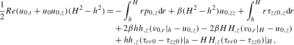
(2.20) \begin{align} v_0=-\frac {r}{2}u_{0,z}+\frac {C(z,t)}{r}, \end{align}

where $C(z,t)$ is an integration function that is determined later using the boundary conditions. The leading-order momentum equations are given by

(2.21) \begin{align} &Re(u_{0,t}+u_0u_{0,z})=-p_{0,z}+\frac {\beta }{r}(ru_{2,r})_{,r}+\frac {\beta }{r}(rv_{0,z})_{,r}+2\beta u_{0,zz}+\frac {1}{r}(r\tau _{rz2})_{,r}+\tau _{zz0,z}, \end{align}

(2.22) \begin{align} &\tau _{rr0,r}+\frac {\tau _{rr0}-\tau _{\theta \theta 0}}{r}-p_{0,r}=0. \end{align}

The leading-order constitutive equations are

(2.23) \begin{align} &\tau _{rr0}+De\big (\mathscr{L}(\tau _{rr0})-2\tau _{rr0}v_{0,r}\big)+\frac {\alpha De}{1-\beta }\tau _{rr0}^2=2(1-\beta)v_{0,r}, \end{align}

(2.24) \begin{align} &\tau _{\theta \theta 0}+De\left (\mathscr{L}(\tau _{\theta \theta 0})-2\tau _{\theta \theta 0}\frac {v_0}{r}\right)+\frac {\alpha De}{1-\beta }\tau _{\theta \theta 0}^2=2(1-\beta)\frac {v_0}{r}, \end{align}

(2.25) \begin{align} &\tau _{zz0}+De\big (\mathscr{L}(\tau _{zz0})-2\tau _{zz0}u_{0,z}\big)+\frac {\alpha De}{1-\beta }\tau _{zz0}^2=2(1-\beta)u_{0,z}, \end{align}

where $\mathscr{L}(\cdot)=(\cdot)_{,t}+v_0(\cdot)_{,r}+u_0(\cdot)_{,z}$ . The leading-order normal components of the dynamic boundary conditions are

(2.26) \begin{align} p_0-2\beta v_{0,r}-\tau _{rr0}=-\frac {1}{{Ca}\, h}\quad \text{at}\quad r=h(z,t), \end{align}

(2.27) \begin{align} p_0-2\beta v_{0,r}-\tau _{rr0}=\frac {1}{{Ca}\, H}\quad \text{at}\quad r=H(z,t). \end{align}

Considering $\mathcal{O}(\epsilon ^2)$ terms of the tangential components of the dynamic boundary conditions (A10)–(A11) gives

(2.28) \begin{align} &2\beta h_{,z}(v_{0,r}-u_{0,z})+\beta u_{2,r}+\beta v_{0,z} +h_{,z}(\tau _{rr0}-\tau _{zz0})+\tau _{rz2}=0\quad \text{at}\quad r=h(z,t), \end{align}

(2.29) \begin{align} &2\beta H_{,z}(v_{0,r}-u_{0,z})+\beta u_{2,r}+\beta v_{0,z} +H_{,z}(\tau _{rr0}-\tau _{zz0})+\tau _{rz2}=0\quad \text{at}\quad r=H(z,t). \end{align}

To obtain a long-wave equation, we multiply (2.21) by $r$ , integrate with respect to $r$ and use (2.28)–(2.29) to obtain

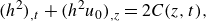
(2.30) \begin{align} \frac {1}{2}Re(u_{0,t}+u_0 u_{0,z})(H^2-h^2)=&-\int _{h}^{H}r p_{0,z}\text{d}r+\beta (H^2-h^2)u_{0,zz}+\int _{h}^{H}r\tau _{zz0,z}\text{d}r\nonumber \\ &+2\beta h h_{,z}(v_{0,r}|_{h}-u_{0,z})-2\beta H H_{,z}(v_{0,r}|_{H}-u_{0,z})\nonumber \\ &+hh_{,z}(\tau _{rr0}-\tau _{zz0})|_{h}-HH_{,z}(\tau _{rr0}-\tau _{zz0})|_{H}, \end{align}

where ‘ $|_{h}$ ’ and ‘ $|_{H}$ ’ denote evaluation at the $r=h$ and $r=H$ boundaries, respectively. Moreover, by substituting (2.20) into the kinematic boundary conditions (2.11), we obtain the equations for $h$ and $H$ :

(2.31) \begin{align} &(h^2)_{,t}+(h^2u_0)_{,z}=2C(z,t), \end{align}

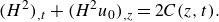(2.32) \begin{align} &(H^2)_{,t}+(H^2 u_0)_{,z}=2C(z,t). \end{align}

Consequently, by using (2.20) to eliminate $v_0$ we obtain a closed system, (2.22)–(2.27) and (2.30)–(2.32), for $u_0,\ h,\ H,\ p_0,\ C,\ \tau _{rr0},\ \tau _{zz0}$ and $\tau _{\theta \theta 0}$ . In the case of a Newtonian fluid, it can be shown that the leading-order pressure $p_0$ is independent of $r$ (Fitt et al. 2002). This allows for a straightforward evaluation of the integrals in (2.30), resulting in a set of three equations for $u_0$ , $h$ and $H$ that are independent of $r$ . However, in the current problem the pressure is not independent of $r$ and it turns out that the integrals in (2.30) cannot be expressed in terms of elementary functions, so one cannot directly derive long-wave equations that are tractable. In the case of solid viscoelastic threads without internal holes, many authors have proceeded by expanding the various dynamic variables as Taylor series in powers of $\epsilon r$ (Bechtel et al. 1988; Forest & Wang 1990; Clasen et al. 2006; Eggers & Villermaux 2008; Li & He 2021). This approach is suitable because the point $r=0$ is included in the domain, so the regularity conditions at $r=0$ preclude terms that are singular. However, in the current problem, $r=0$ is not part of the domain, which means that terms arising from the $C/r$ term in (2.20) cannot be accurately described using a Taylor series expansion. In fact, if one attempts to expand in powers of $\epsilon r$ , one immediately sees that such an expansion cannot be compatible with the normal boundary conditions (2.26)–(2.27). Therefore, an alternative method is needed to derive the long-wave equations.

3. Low-Deborah-number asymptotics

In this section, we simplify our system of equations and boundary conditions, (2.22)–(2.27) and (2.30)–(2.32), using the small-Deborah-number assumption. On examination of (2.20), (2.22), (2.23) and (2.25), we observe that the elastic stresses depend on $r$ and are strongly coupled with the pressure $p_0$ and velocity $u_0$ . This makes it challenging to deal with the integrals in (2.30). In order to overcome this challenge and obtain long-wave equations, we consider the weakly viscoelastic limit, ${De}\ll 1$ . Actually, many works consider the weakly viscoelastic limit for various problems and a broad range of important results have been found using such techniques (De Corato, Greco & Maffettone 2015; Zhou et al. 2016; Datt & Elfring 2019; Binagia et al. 2020; Boyko & Stone 2022; Boyko & Christov 2023). Following their methodology, we pose an expansion of the form

(3.1) \begin{align} \psi =\psi ^{(0)}+De\psi ^{(1)}+\mathcal{O}(De^2), \end{align}

where $\psi$ represents the quantities $\boldsymbol{\tau }_0,\ p_0,\ \boldsymbol{u}_0,\ h,\ H$ and $C$ .

The derivation of the leading-order long-wave equations in $De$ is presented in Appendix B. These equations (B8)–(B12) are equivalent to setting $De=0$ and are therefore the same as the equations for a Newtonian fluid tube with viscosity $\eta _0$ . The system is therefore essentially equivalent to that derived in Fitt et al. (2002). To include elastic effects in our model we must consider the next-order terms in $De$ .

3.1. First-order long-wave equations in $De$

Taking the first-order terms in $De$ of (2.20), we obtain

(3.2) \begin{align} v^{(1)}_0=-\frac {r}{2}u^{(1)}_{0,z}+\frac {C^{(1)}(z,t)}{r}. \end{align}

The constitutive relations (2.23)–(2.25) yield

(3.3) \begin{align} &\tau ^{(1)}_{rr0}=2(1-\beta)v^{(1)}_{0,r}-\left (\mathscr{L}^{(0)}(\tau ^{(0)}_{rr0})-2\tau ^{(0)}_{rr0}v^{(0)}_{0,r}\right)-\frac {\alpha }{1-\beta }\tau ^{(0)2}_{rr0}, \end{align}

(3.4) \begin{align} &\tau ^{(1)}_{\theta \theta 0}=2(1-\beta)\frac {v^{(1)}_0}{r}-\left (\mathscr{L}^{(0)}(\tau ^{(0)}_{\theta \theta 0})-2\tau ^{(0)}_{\theta \theta 0}\frac {v^{(0)}_{0}}{r}\right)-\frac {\alpha }{1-\beta }\tau ^{(0)2}_{\theta \theta 0}, \end{align}

(3.5) \begin{align} &\tau ^{(1)}_{zz0}=2(1-\beta)u^{(1)}_{0,z}-\left (\mathscr{L}^{(0)}(\tau ^{(0)}_{zz0})-2\tau ^{(0)}_{zz0}u^{(0)}_{0,z}\right)-\frac {\alpha }{1-\beta }\tau ^{(0)2}_{zz0}, \end{align}

where $\mathscr{L}^{(0)}(\cdot)=(\cdot)_{,t}+v^{(0)}_0(\cdot)_{,r}+u^{(0)}_0(\cdot)_{,z}$ . Using (2.22), we obtain

(3.6) \begin{align} p^{(1)}_{0,r}=\frac {1}{r}\left (r \tau ^{(1)}_{rr0}\right)_{,r}-\frac {1}{r}\tau ^{(1)}_{\theta \theta 0}. \end{align}

Integrating (3.6) with respect to $r$ yields

(3.7) \begin{align} p^{(1)}_0=\int \frac {1}{r}\left (r \tau ^{(1)}_{rr0}\right)_{,r} \text{d}r- \int \frac {1}{r}\tau ^{(1)}_{\theta \theta 0} \text{d}r +A^{(1)}(z,t), \end{align}

where $A^{(1)}(z,t)$ is an integration function that is determined later using the first-order normal boundary conditions that are given by

(3.8) \begin{align} &p^{(1)}_0-2\beta v^{(0)}_{0,rr}h^{(1)}-2\beta v^{(1)}_{0,r}-\tau ^{(0)}_{rr0,r}h^{(1)}-\tau ^{(1)}_{rr0}=\frac {h^{(1)}}{{Ca}\, h^{(0)2}}\quad \text{at}\quad r=h^{(0)}, \end{align}

(3.9) \begin{align} &p^{(1)}_0-2\beta v^{(0)}_{0,rr}H^{(1)}-2\beta v^{(1)}_{0,r}-\tau ^{(0)}_{rr0,r}H^{(1)}-\tau ^{(1)}_{rr0}=-\frac {H^{(1)}}{{Ca}\, H^{(0)2}}\quad \text{at}\quad r=H^{(0)}. \end{align}

We note that (3.8) and (3.9) form an algebraic system for $A^{(1)}(z,t)$ and $C^{(1)}(z,t)$ , which can be solved to give

(3.10) \begin{align} A^{(1)}(z,t)=&-u^{(1)}_{0,z}+\frac {h^{(1)}-H^{(1)}}{{Ca}(H^{(0)}-h^{(0)})^2}+\frac {2(1-\beta)C^{(0)2}}{h^{(0)2}H^{(0)2}} \nonumber \\ & +(1-\beta)\left [(1-\alpha)u^{(0)2}_{0,z}+u^{(0)}_{0,zt} + u^{(0)}_0u^{(0)}_{0,zz}\right], \end{align}

(3.11) \begin{align} C^{(1)}(z,t)=&\frac {h^{(0)2}H^{(1)}-H^{(0)2}h^{(1)}}{2{Ca}(H^{(0)}-h^{(0)})^2} \nonumber \\ &\quad +(\beta -1)\left [\frac {(h^{(0)2}+H^{(0)2})C^{(0)2}}{h^{(0)2}H^{(0)2}}-(C^{(0)}_{,t}+u^{(0)}_0C^{(0)}_{,z}) +(2\alpha -3)C^{(0)}u^{(0)}_{0,z}\right]. \end{align}

Hence, we can use (3.2)–(3.5) and (3.10)–(3.11) to express $v^{(1)}_0,\ \tau ^{(1)}_{rr0},\ \tau ^{(1)}_{\theta \theta 0},\ \tau ^{(1)}_{zz0},\ A^{(1)}$ and $C^{(1)}$ in terms of the leading-order quantities $u^{(0)}_0,\ h^{(0)},\ H^{(0)}$ and $C^{(0)}$ . Although the physical meaning of most variables is clear, the physical interpretation of $C(z,t)=C^{(0)}(z,t)+{De}\, C^{(1)}(z,t)$ warrants some discussion. It is readily shown from (B7) and (3.11) that $C$ , which first appeared in (2.20), will be identically zero in the case of zero surface tension ( ${Ca}=\infty$ ). In fact, the radial velocity $v_0$ in (2.20) is composed of two parts: $-r u_{0,z}/2$ , which arises from axial stretching and mass conservation, and $C/r$ , which arises from surface tension acting on the inner and outer boundaries. Thus, the quantity $C$ represents the strength of the radial flow induced by surface tension.

Considering the terms of $\mathcal{O}(De)$ in the axial momentum equation (2.30), we get integrals that are straightforward to evaluate and obtain

(3.12) \begin{align} &\frac {1}{2}Re(u^{(1)}_{0,t}{+}u^{(1)}_0 u^{(0)}_{0,z}{+}u^{(0)}_0 u^{(1)}_{0,z})(H^{(0)2}{-}h^{(0)2}) =-Re (u^{(0)}_{0,t}{+} u^{(0)}_0u^{(0)}_{0,z})(H^{(0)}H^{(1)}{-}h^{(0)}h^{(1)})\nonumber \\ &-A^{(0)}_{,z}(H^{(0)}H^{(1)}-h^{(0)}h^{(1)})+2(2\alpha -1)(\beta -1)C^{(0)}C^{(0)}_{,z}\left (\frac {1}{H^{(0)2}}-\frac {1}{h^{(0)2}}\right)\nonumber \\ &+\left (\beta u^{(1)}_{0,zz}+\frac {1}{2}\tau ^{(1)}_{zz0,z}-\frac {1}{2}A^{(1)}_{,z}\right)(H^{(0)2}-h^{(0)2})\nonumber \\ & +\left (2\beta u^{(0)}_{0,zz}+\tau ^{(0)}_{zz0,z}\right)(H^{(0)}H^{(1)}-h^{(0)}h^{(1)})\nonumber \\ &+\left [2\beta (v^{(0)}_{0,r}-u^{(0)}_{0,z})+(\tau ^{(0)}_{rr0}-\tau ^{(0)}_{zz0})\right]\left |_{h^{(0)}}(h^{(1)}h^{(0)}_{,z}+h^{(0)}h^{(1)}_{,z})\right.\nonumber \\ &+\left.\left [2\beta (v^{(1)}_{0,r}-u^{(1)}_{0,z})+(\tau ^{(1)}_{rr0}-\tau ^{(1)}_{zz0})\right]\right |_{h^{(0)}}h^{(0)}h^{(0)}_{,z}\nonumber \\ &-\left.\left [2\beta (v^{(1)}_{0,r}-u^{(1)}_{0,z})+(\tau ^{(1)}_{rr0}-\tau ^{(1)}_{zz0})\right]\right |_{H^{(0)}}H^{(0)}H^{(0)}_{,z}\nonumber \\ &-\left.\left [2\beta (v^{(0)}_{0,r}-u^{(0)}_{0,z})+(\tau ^{(0)}_{rr0}-\tau ^{(0)}_{zz0})\right]\right |_{H^{(0)}}(H^{(1)}H^{(0)}_{,z}+H^{(0)}H^{(1)}_{,z}). \end{align}

Considering the terms of $\mathcal{O}(De)$ in (2.31)–(2.32), we obtain

(3.13) \begin{align} &2(h^{(0)} h^{(1)})_{,t}+2(h^{(0)} h^{(1)} u^{(0)}_0)_{,z}+(h^{(0)2} u^{(1)}_0)_{,z}=2C^{(1)}, \end{align}

(3.14) \begin{align} &2(H^{(0)} H^{(1)})_{,t}+2(H^{(0)} H^{(1)} u^{(0)}_0)_{,z}+(H^{(0)2} u^{(1)}_0)_{,z}=2C^{(1)}. \end{align}

Substituting (3.1) into (A12)–(A13), we obtain boundary conditions for $u^{(1)}_0$ , $h^{(1)}$ and $H^{(1)}$ , namely

(3.15) \begin{align} u^{(1)}_0&=0,\quad h^{(1)}=0,\quad H^{(1)}=0\quad \text{at}\quad z=0, \end{align}

(3.16) \begin{align} u^{(1)}_0&=0\quad \text{at}\quad z=1. \end{align}

As mentioned above, (B7)–(B12) represent the long-wave equations for a Newtonian fluid. We must first solve these equations to obtain $u^{(0)}_0,\ h^{(0)}$ and $H^{(0)}$ , after which we substitute these solutions into (3.2), (3.3), (3.5) and (3.10)–(3.16), which represent equations for $u^{(1)}_0,\ h^{(1)}$ and $H^{(1)}$ . The quantities $u^{(1)}_0,\ h^{(1)}$ and $H^{(1)}$ capture the leading-order effects of elastic stresses and describe the variation from the zero-Deborah-number flow. We note that in the limit $\beta \to 1$ , the quantities $u^{(1)}_0,\ h^{(1)}$ and $H^{(1)}$ tend to zero. This is because the limit $\beta \to 1$ corresponds to the case $\eta _p\to 0$ that represents no polymeric effect on the flow, which is therefore purely Newtonian.

4. Numerical method for steady-state equations

In this section, we consider the steady state by setting $\partial _{t}\equiv 0$ in (B7)–(B12) and (3.12)–(3.16). In order to numerically obtain the steady-state solutions, we note that (B8) is a second-order ordinary differential equation (ODE) for the quantity $u^{(0)}_0$ , and (B9)–(B10) are two first-order ODEs for $h^{(0)}$ and $H^{(0)}$ . We also have three boundary conditions at $z = 0$ and one boundary condition at $z = 1$ . Therefore, this system can be readily solved using a shooting method in which one starts with a guessed value of $u^{(0)}_{0,z}$ at $z = 0$ , then solves (B8)–(B10) numerically using a standard ODE solver (e.g. MATLAB function ‘ode45’) subject to the ‘initial’ conditions (B11), and employs a root-finding technique (e.g. MATLAB function ‘fzero’) to find $u^{(0)}_{0,z}$ at $z = 0$ such that the condition (B12) is satisfied. Similarly, (3.12)–(3.14) are solved by guessing the value of $u^{(1)}_{0,z}$ and employing a root-finding technique to achieve (3.16). Consequently, we can readily solve $u_0,h$ and $H$ numerically up to $\mathcal{O}(De)$ .

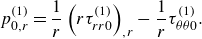
4.1. Results of steady state

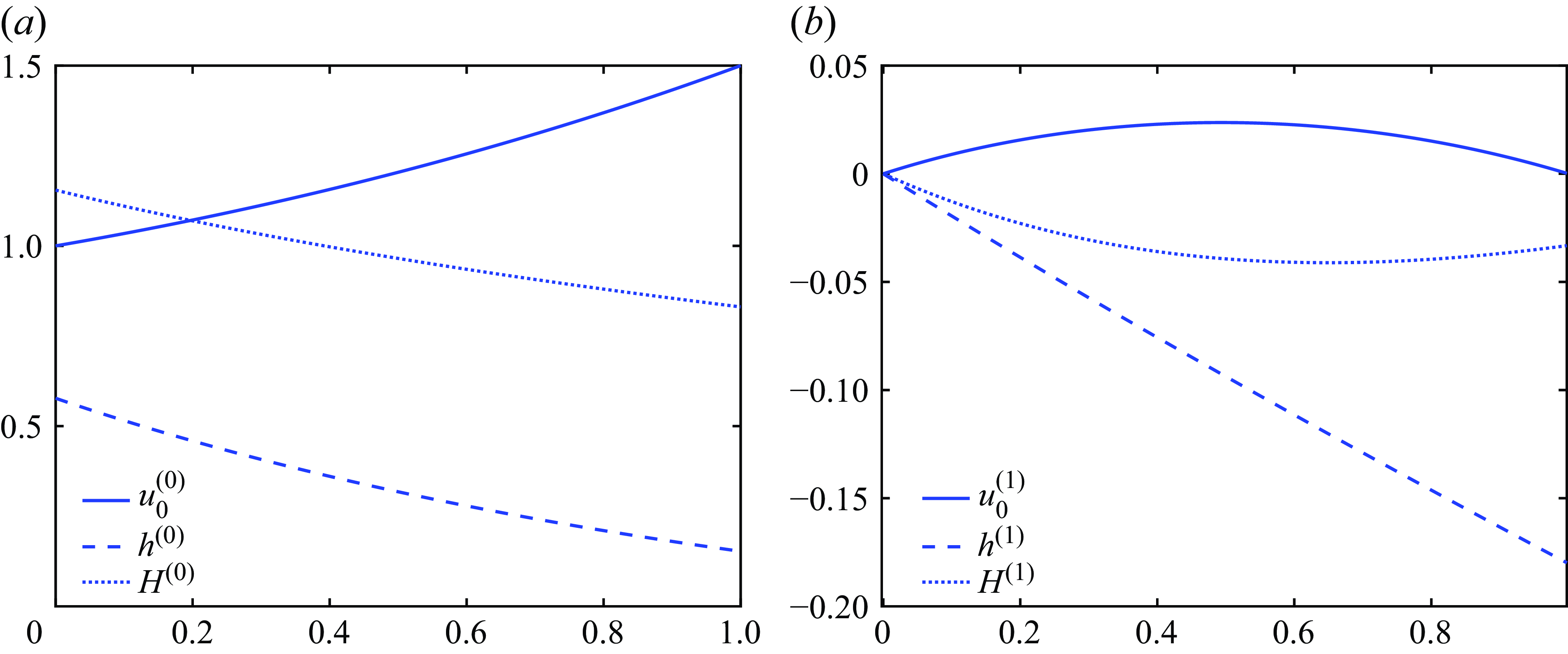
Figure 2. (a) The velocity $u^{(0)}_0$ , the hole radius $h^{(0)}$ and the outer radius $H^{(0)}$ for a Newtonian fluid versus the axial distance $z$ . (b) The corrections $u^{(1)}_0$ , $h^{(1)}$ and $H^{(1)}$ to the Newtonian flow due to elastic effects. The parameters are $D=1.5,\ Ca=1.8,\ Re=0,\ \phi =0.5,\ \alpha =0$ and $\beta =0.1$ .

The profiles for $u^{(0)}_0,\ h^{(0)},\ H^{(0)}$ and $u^{(1)}_0,\ h^{(1)},\ H^{(1)}$ are plotted in figure 2 for a typical set of parameter values. Other parameters give broadly similar behaviour. Figure 2(a) is the leading-order velocity, hole size and outer radius, which are the same as those for a Newtonian fluid. As a result, $u^{(0)},\ h^{(0)}$ and $H^{(0)}$ are independent of the parameters $\alpha$ and $\beta$ , which characterise elasticity in the constitutive relation. Figure 2(b) represents the $\mathcal{O}(De)$ corrections to the Newtonian flow. The velocities at both inlet nozzle and take-up point are fixed, resulting in $u^{(1)}_0$ being zero at both the inlet nozzle and take-up point, but $u^{(1)}_0$ is positive in the bulk meaning that elastic effects act to increase the velocity. Figure 2 shows that the elasticity acts to reduce the hole size since $h^{(1)}$ is negative. The elasticity also contributes to a reduction of the outer radius, but this is significantly weaker than the effect on the hole size. It is worth noting that the hole size at the take-up point is one of the most important factors in the production of holey fibres, since the geometry at the take-up point represents the output of the drawing device. As we described in the introduction, the optical properties of fibres can depend very sensitively on the output geometry. Therefore, the most important quantities from a manufacturing perspective are $h$ and $H$ at the take-up point $z=1$ . Furthermore, we note from (A12) and (2.31)–(2.32) that

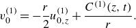
(4.1) \begin{align} (H^2-h^2)u_0=1, \end{align}

for the steady state. Expanding (4.1) with respect to $De$ and equating the terms of first order in $De$ , we obtain

(4.2) \begin{align} 2(H^{(0)}H^{(1)}-h^{(0)}h^{(1)})u^{(0)}_0+(H^{(0)2}-h^{(0)2})u^{(1)}_0=0. \end{align}

Evaluating (4.2) at $z=1$ , we obtain

(4.3) \begin{align} \frac {H^{(1)}}{h^{(1)}}=\frac {h^{(0)}}{H^{(0)}}\quad \text{at}\quad z=1. \end{align}

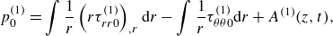
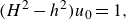
Figure 3. The effect of elasticity on the hole size at the take-up point, $h^{(1)}(z=1)$ , versus the ratio of inner to outer radius at the inlet nozzle, $\phi$ , for different values of the draw ratio $D$ . Other parameters are $Ca=1.8,\ Re=0,\ \alpha =0$ and $\beta =0.1$ .

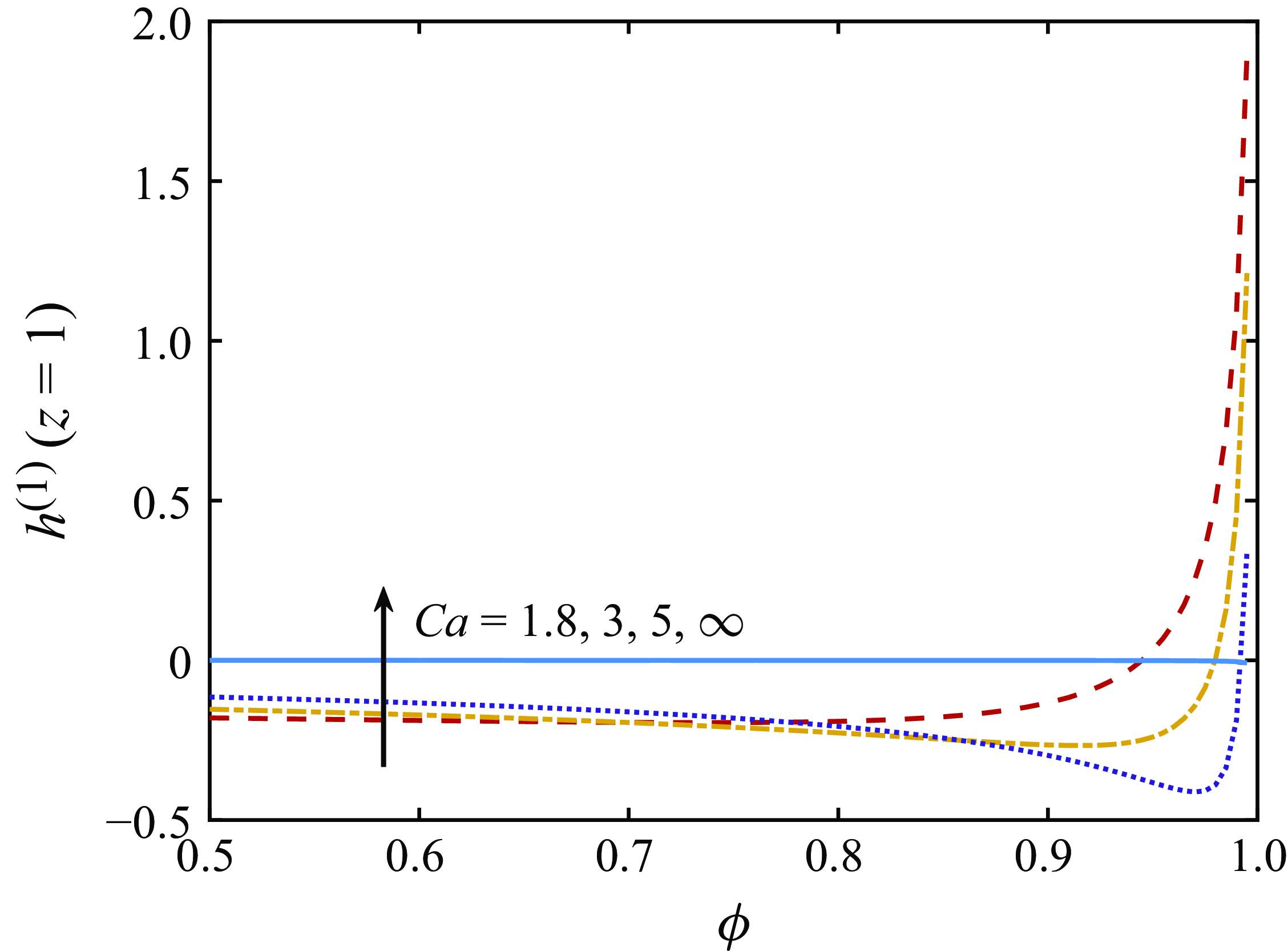
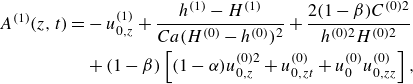
Figure 4. The effect of elasticity on the hole size at the take-up point, $h^{(1)}(z=1)$ , versus the ratio of inner to outer radius at the inlet nozzle, $\phi$ , for different values of the capillary number $Ca$ . Other parameters are $D=1.5,\ Re=0,\ \alpha =0$ and $\beta =0.1$ .

Thus, we can determine $H^{(1)}$ at the take-up point once $h^{(1)}$ is known. Therefore, we focus on $h^{(1)}(z=1)$ that represents the effect that elasticity has on the hole size at the take-up point in the subsequent analysis. In figures 3 and 4 we explore how the hole size at the take-up point $h^{(1)}(z=1)$ depends on the inlet hole size by plotting $h^{(1)}(z=1)$ as a function of $\phi$ , recalling that $\phi$ represents the ratio of inner radius to outer radius at the inlet nozzle. Note that these figures are for sufficiently large $\phi$ ( $\geqslant 0.5$ ) such that hole closure ( $h^{(0)}=0$ ) does not occur. Hole closure can occur for small $\phi$ , but in fibre drawing this is, perhaps with a very few exceptions, always undesirable, since if a solid thread is desired it can be more easily obtained by using a solid thread at the inlet nozzle. Therefore, in this study, we do not consider hole closure and only focus on the dynamics for sufficiently large $\phi$ such that hole closure does not occur. We plot the curves for different $D$ and $Ca$ in figures 3 and 4. Figure 3 shows that an increase in $D$ enhances the hole closure at the take-up point due to elasticity. For very weak drawing corresponding to $D=1.1$ , $h^{(1)}(z=1)$ is always positive and becomes more positive as $\phi$ increases, indicating that the elasticity always plays a role in increasing the hole size. However, for moderate drawing, with $D=1.5,\ 3$ and $5$ , we observe that $h^{(1)}(z=1)$ is initially negative and decreases with $\phi$ , indicating that the effect of elasticity in decreasing the hole size at the take-up point becomes stronger as $\phi$ increases. However, for sufficiently large $\phi$ , we see the opposite. This phenomenon can be also observed in the red curve in figure 4 for $Ca=1.8$ and $D=1.5$ . Therefore, roughly speaking, there are two different types of behaviour that can be observed in the plots: one where $\phi$ is close to $1$ , which we refer to as the ‘large hole size’ case, and another where $\phi$ is not close to $1$ , which we refer to as the ‘moderate hole size’ case. The subsequent sections concentrate on examining these two cases. Furthermore, figure 4 shows that for sufficiently small values of $\phi$ an increase in $Ca$ will decrease the hole closure at the take-up point due to elasticity. However, the opposite trend is observed for sufficiently large values of $\phi$ . In addition, as $Ca\to \infty$ , (B7) and (3.11) imply that $C^{(0)}$ and $C^{(1)}$ will tend to zero, and one can integrate the steady version of (3.13) from $z=0$ to $z=1$ to see that $h^{(1)}(z=1)=0$ . Hence, the hole size at the take-up point for viscoelastic fluids will tend to that for a Newtonian fluid and hence $h^{(1)}(z=1)$ will tend to zero as $Ca\to \infty$ , as shown in figure 4.

4.1.1. Moderate and large hole sizes

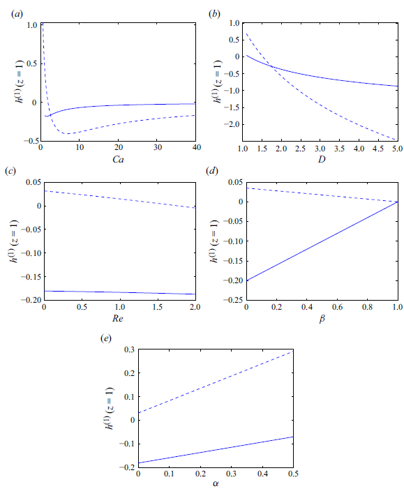
Figure 5. The effect of elasticity on the hole size at the take-up point versus (a) capillary number $Ca$ , (b) draw ratio $D$ , (c) Reynolds number $Re$ , (d) solvent to bulk viscosity $\beta$ and (e) mobility factor $\alpha$ . The solid curve is for $\phi =0.5$ , the dashed curve is for $\phi =0.95$ . In (a), other parameters are $D=1.5,$ $Re=0$ , $\alpha =0$ and $\beta =0.1$ . In (b), other parameters are $Re=0$ , $Ca=1.8$ , $\alpha =0$ and $\beta =0.1$ . In (c), other parameters are $D=1.5,$ $Ca=1.8$ , $\alpha =0$ and $\beta =0.1$ . In (d), other parameters are $D=1.5$ , $Ca=1.8,$ $Re=0$ and $\alpha =0$ . In (e), other parameters are $D=1.5$ , $Ca=1.8$ , $Re=0$ and $\beta =0.1$ .

In figure 5, we compare the hole closure at the take-up point due to elasticity for moderate ( $\phi =0.5$ ) and large ( $\phi =0.95$ ) inlet hole sizes. In particular, we examine how the various parameters $Ca,\ D,\ Re,\ \beta $ and $\alpha$ affect $h^{(1)}(z=1)$ . In figure 5(a), we examine the effect of capillary number (Ca). Here, we start with $Ca\approx 1.1$ for the case of a moderate hole size and $Ca\approx 0.6$ for the case of a large hole size, as the hole will close for smaller capillary numbers corresponding to very strong surface tension. For the moderate value of $\phi$ (solid curve), $h^{(1)}(z=1)$ is always negative indicating that the hole size at the take-up point is consistently smaller than for a pure Newtonian fluid. For large $\phi$ (dashed curve) and sufficiently small Ca, $h^{(1)}(z=1)$ is positive indicating that the hole size at the take-up point is larger than the Newtonian one. Furthermore, we note that $h^{(1)}(z=1)$ is not a monotonic function of Ca. For sufficiently small Ca, $h^{(1)}(z=1)$ reduces as Ca increases. However, this trend reverses beyond a critical value of Ca. This non-monotonic behaviour can also be observed in figure 4. As shown in figure 4, $h^{(1)}(z=1)\to 0$ when $Ca\to \infty$ (negligible surface tension) for all $\phi$ .

Figure 5(b) shows the effect of draw ratio D and that there is a critical value of D above which elastic effects decrease and below which elastic effects increase the hole size at the take-up point. For the moderate value of $\phi$ (solid curve) elastic effects only act to very weakly increase the hole size for values of D quite close to $1$ . Whereas, for the large value of $\phi$ (dashed curve) the effect is much stronger and acts over a larger range of D values. An increase in the draw ratio uniformly enhances the hole closure at the take-up point due to elasticity. This phenomenon can also be observed in figure 3.

The effect of inertia is shown in figure 5(c). For $\phi =0.5$ (solid curve), we observe that $h^{(1)}(z=1)$ is always negative indicating that elastic effects enhance hole closure at the take-up point. On the other hand, for $\phi =0.95$ (dashed curve) we observe that $h^{(1)}(z=1)$ is positive for $Re\lesssim 1.8$ , indicating that elastic effects suppress hole closure. However, for $Re\gtrsim 1.8$ we see that the opposite is true. Nevertheless, as Re varies the effect on $h^{(1)}(z=1)$ is relatively weak.

Figure 5(d) shows how $\beta$ (solvent to bulk viscosity ratio) affects $h^{(1)}(z=1)$ . We note that the maximum value that $\beta$ can approach is $1$ , and this corresponds to a purely Newtonian fluid (only solvent). Therefore, as $\beta$ tends to unity, the elastic effects will tend to zero and we will get $h^{(1)}(z=1)\to 0$ . For $\phi =0.5$ , $h^{(1)}(z=1)$ is negative, indicating that the elasticity acts to enhance hole closure. As $\beta$ increases, the effect of elasticity becomes weaker. While for $\phi =0.95$ , $h^{(1)}(z=1)$ is positive, indicating that the elasticity suppresses hole closure. As $\beta$ increases towards unity the effects of elasticity on the hole closure monotonically decrease to zero.

In figure 5(e) we show how $\alpha$ (mobility factor) affects $h^{(1)}(z=1)$ . We note that in the Giesekus model, physical constraints demand that $\alpha \lt 0.5$ (Morozov & Spagnolie 2015). For $\phi =0.5$ elastic effects enhance hole closure, but this becomes weaker as $\alpha$ increases. On the other hand, elastic effects suppress hole closure for $\phi =0.95$ and this suppression becomes stronger as $\alpha$ increases. We return to this phenomenon in the next subsection.

4.2. Assessing the effects of different contributions to the hole size at the take-up point

It is well known that elastic effects suppress the surface-tension-driven pinching that occurs for threads without holes (Entov & Hinch 1997; Li & Fontelos 2003). Therefore, one might guess that elastic effects will suppress the surface-tension-driven hole closure that occurs for threads with holes. However, from figures 3 and 4, we surprisingly found that elastic effects enhance hole closure, provided $\phi$ is not too large and D is not close to unity. On the other hand, for threads with large initial hole size or draw ratio D close to unity, the elasticity has the opposite effect. To provide further insight into this behaviour, we elucidate the relative importance of different contributions to $h^{(1)}(z=1)$ . We remind the reader that the radial flow is of the form $v_0=-r u_{0,z}/2+C/r$ , where $C$ represents the strength of the radial flow induced by surface tension forces, which we expanded as an asymptotic series in terms of the Deborah number, $C=C^{(0)}+{De}\,C^{(1)}$ . Here, $C^{(0)}$ represents the strength of the radial flow induced by surface tension for zero Deborah number and $C^{(1)}$ represents the correction to this radial flow that arises from elastic effects. The inner surface must necessarily have larger curvature than the outer surface, and this will generate an inward flow meaning that $C^{(0)}\lt 0$ .

At leading order, the inward surface tension forces generate a flow that is opposed by viscous stresses. By considering the leading-order $r-$ momentum equation (2.22) and normal dynamic boundary conditions (2.26)–(2.27) we obtain

(4.4) \begin{align} \int _{h^{(0)}}^{H^{(0)}}\frac {N^{(0)}_2}{r}\text{d}r=\frac {1}{Ca}\left(\frac {1}{h^{(0)}}+\frac {1}{H^{(0)}}\right), \end{align}

where $N^{(0)}_2=\sigma ^{(0)}_{rr0}-\sigma ^{(0)}_{\theta \theta 0}$ is the second normal stress difference to leading order in $De$ , with $\sigma ^{(0)}_{rr0}=-p+2\beta v^{(0)}_{0,r}+\tau ^{(0)}_{rr0}$ and $\sigma ^{(0)}_{\theta \theta 0}=-p+2\beta v^{(0)}_0/r+\tau ^{(0)}_{\theta \theta 0}$ . Equation (4.4) shows that, at leading order, the surface tension force is balanced purely by the second normal stress difference.

By setting $\partial _t\equiv 0$ and integrating (3.13) with respect to $z$ , we obtain

(4.5) \begin{align} h^{(1)}(z=1)=\frac {1}{h^{(0)}(z=1)D} \int _{0}^{1} C^{(1)}\text{d}z. \end{align}

This shows that $h^{(1)}(z=1)$ is directly determined by the elastic correction to the surface-tension-driven radial flow. In some sense (4.5) simply reflects the fact that an increased inward radial flow due to elastic effects will combine with the kinematic condition (2.11) to enhance hole closure.

In order to understand the physical mechanism that is associated with $C^{(1)}$ , we subtract the two first-order normal boundary conditions (3.8) and (3.9). Then using (3.2) and (3.7), and integrating by parts, we obtain

(4.6) \begin{align} C^{(1)}=\frac {h^{(0)2} H^{(0)2}}{2\beta (H^{(0)2}-h^{(0)2})}\int _{h^{(0)}}^{H^{(0)}}\frac {T^{(1)}_2}{r}\text{d}r+\frac {h^{(0)2} H^{(1)}-H^{(0)2}h^{(1)}}{2 \beta {Ca}(H^{(0)}-h^{(0)})^2}, \end{align}

where we define $T_2=\tau _{rr0}-\tau _{\theta \theta 0}$ to be the elastic component of the second normal stress difference and expand $T_2$ in the form $T_2=T_2^{(0)}+{De}\, T_2^{(1)}$ . This equation shows that the elastic correction to $C^{(1)}$ and hence the hole size at the take-up point only depend on the stress via $T^{(1)}_2$ . Second normal stress differences are often ignored in viscoelastic flows, because first normal stress differences are generally more important. Nevertheless, Maklad & Poole (2021) give a very complete description of their importance and the specific physical role they can play. As we can see in (4.6) the effect of elasticity on hole evolution is directly related to the second normal stress difference and is independent of the first normal stress difference.

We note that (4.6) contains two terms on the right-hand side. The first term involves the elastic component of the second normal stress difference, while the second term comes from the linearised surface tension terms in (3.8) and (3.9) that arise from expanding $h$ and $H$ as a series in $De$ . This second term does not directly involve the elastic stresses and is therefore simply a response to the elastic forces rather than a driving mechanism for the evolution of the hole.

Equations (3.3)–(3.4) show how the first-order corrections to the elastic component of the second normal stress difference, given by $T^{(1)}_2$ , arise as an elastic response to the stresses generated by $\tau ^{(0)}_{rr0}$ and $\tau ^{(0)}_{\theta \theta 0}$ for the zero-Deborah-number flow. We can then use (B2)–(B3) and (3.3)–(3.4) to rewrite $C^{(1)}$ in the form

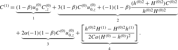(4.7) \begin{align} C^{(1)}&=\underbrace {(1-\beta)u^{(0)}_0 C^{(0)}_{,z}}_{\unicode {x2460}}+\underbrace {3(1-\beta)C^{(0)}u^{(0)}_{0,z}+(-1)(1-\beta)\frac {(h^{(0)2}+H^{(0)2})C^{(0)2}}{h^{(0)2}H^{(0)2}}}_{\unicode {x2461}}\nonumber \\ &\quad +\underbrace {2\alpha (-1)(1-\beta)C^{(0)}u^{(0)}_{0,z}}_{\unicode {x2462}}+\underbrace {\left [\frac {h^{(0)2}H^{(1)}-H^{(0)2}h^{(1)}}{2{Ca}(H^{(0)}-h^{(0)})^2}\right]}_{\unicode {x2463}}. \end{align}

Equation (4.7) shows that $C^{(1)}$ arises from complicated interactions between the upper-convected derivative and the full stress tensor. We have labelled different terms in (4.7) to help us understand the mechanism that drives hole evolution. Terms ${\unicode {x2460}},\ {\unicode {x2461}}$ and $\unicode {x2462}$ all contain $C^{(0)}$ which represents the strength of the radial flow induced by surface tension in the zero-Deborah-number-flow limit. As explained above, $C^{(0)}$ will always be negative and represents an inward flow. In this physical description, we only focus on how the radial flow associated with $C^{(0)}$ induces leading-order elastic stresses, and how this affects $C^{(1)}$ . The radial velocity associated with axial stretching (the $-r u^{(0)}_{0,z}/2$ term in (B1)) can be dealt with in a similar way.

In order to understand how elastic effects play a role in the evolution of the hole size we consider the constitutive relations (3.3)–(3.4) that represent the $\mathcal{O}(De)$ corrections to the stresses. These equations show that the leading-order stresses are advected by the zero-Deborah-number flow in both axial and radial directions and this advection causes changes to the stress. The constitutive relations indicate that these changes will be opposed by $\mathcal{O}(De)$ elastic stresses $\tau ^{(1)}_{rr0}$ , $\tau ^{(1)}_{\theta \theta 0}$ . To understand the physical origin of the terms in (4.7) we need to examine the radial and axial advection terms that give rise to $\mathcal{O}(De)$ elastic stresses. We begin by considering the radial advection. In the zero-Deborah-number approximation, surface tension induces a radial velocity of the form $C^{(0)}/r$ (see (B1)), with $C^{(0)}\lt 0$ . Using (B1)–(B3) we see that the leading-order second normal stress difference $N_2^{(0)}$ that opposes this radial flow is in the positive $r$ direction and decreases as $r$ increases. Hence, the radially inward advective flow will move fluid particles from low positive stress to high positive stress and thus increases the stress. At $\mathcal{O}(De)$ , the elastic response $T^{(1)}_2$ will oppose this stress increase and thus will be negative. Therefore, this effect means that elastic effects associated with radial advection make the hole smaller. This along with the other terms in the upper-convected derivative represents the physical origin of term $\unicode {x2461}$ in (4.7).

We next consider axial advection which advects in the positive $z$ direction since $u^{(0)}_0\gt 0$ . Using (B1)–(B3) we see that the leading-order second normal stress difference is positive and proportional to $C^{(0)}$ . If $C^{(0)}_{,z}\gt 0$ , then axial advection terms will move fluid particles from regions of large positive stress to regions of low positive stress, and thus reduce the stress. At $\mathcal{O}(De)$ , elastic stresses will oppose this change in stress and so the elastic response $T^{(1)}_2$ will be positive. This means that elastic effects associated with axial advection act to make the hole larger if $C^{(0)}_{,z}\gt 0$ . This is the physical origin of term $\unicode {x2460}$ in (4.7).

Term $\unicode {x2462}$ arises from the quadratic nonlinear terms in the Giesekus model. Term $\unicode {x2463}$ is similar to the second term in (4.6), does not directly involve elastic stresses and can be thought of as a response to the elastic mechanism. In order to determine which of the terms dominates we plot the sizes of each of the four terms in figures 6 and 7 for moderate hole size and large hole size, respectively.

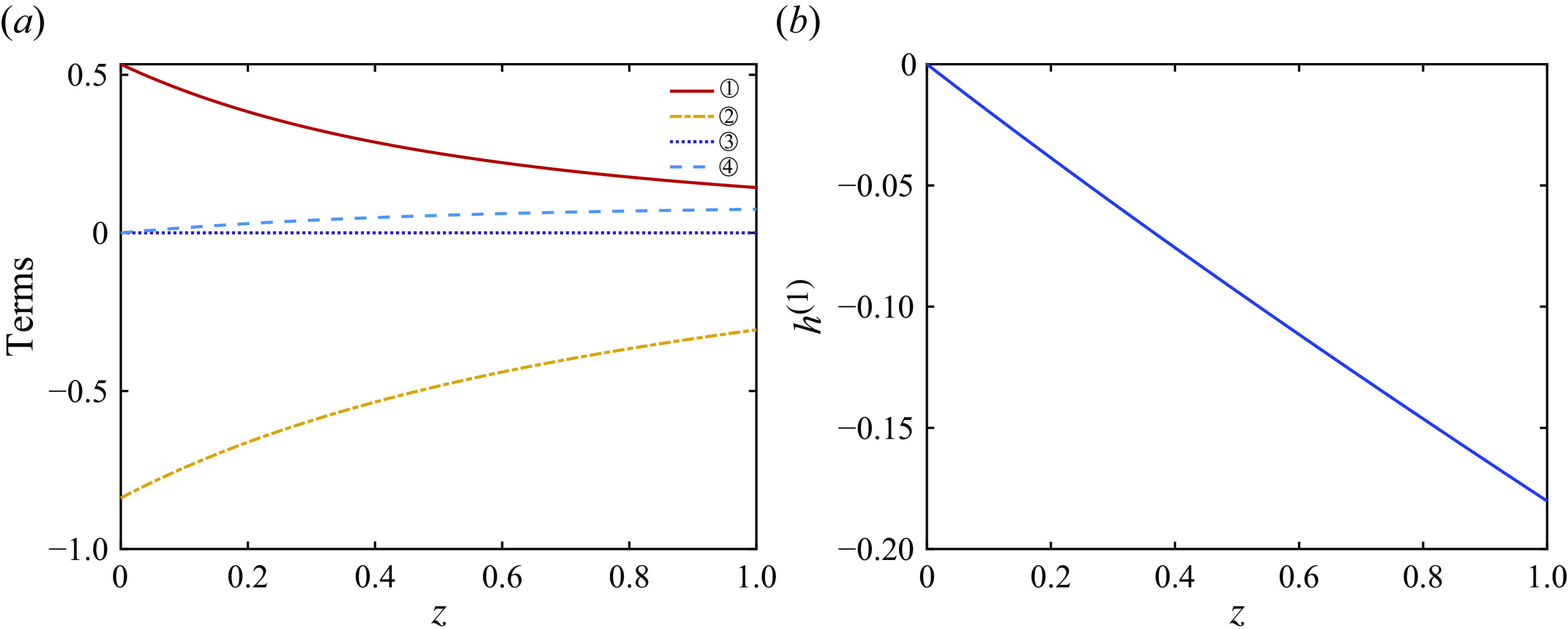
Figure 6. (a) The terms $\unicode {x2460}{-}\unicode {x2463}$ in (4.7) and (b) $h^{(1)}$ versus $z$ for $D=1.5,\ Ca=1.8,\ \phi =0.5,\ Re=0,$ $\alpha =0,\ \beta =0.1$ .

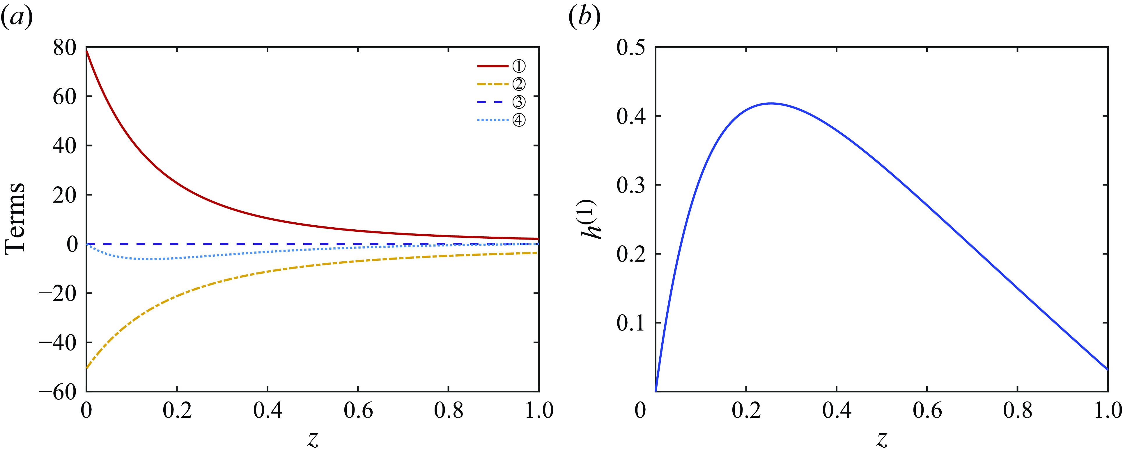
Figure 7. (a) The terms $\unicode {x2460}{-}\unicode {x2463}$ and (b) $h^{(1)}$ versus $z$ for $D=1.5,\ Ca=1.8,\ \phi =0.95,\ Re=0,\ \alpha =0$ , $\beta =0.1$ .

In the case of moderate hole size, figure 6(a) shows that $\unicode {x2461}$ plays the dominant role in causing the integrand $C^{(1)}$ in (4.5) to be negative. Then the first-order second normal stress difference $T^{(1)}_2$ is negative and drives a radially inward flow. This, in turn, leads to $h^{(1)}(z=1)\lt 0$ , as shown in figure 6(b). In summary, for moderate hole size, hole closure is enhanced by elastic effects due to radial advection of stresses arising from the surface-tension-driven flow.

In the case of large hole size, we observe opposite effects of elasticity on the hole size at the take-up point, as illustrated in figures 3 and 4, where $h^{(1)}(z=1)$ is positive. We also analyse the individual terms in (4.7) to explain this phenomenon, which is depicted in figure 7. In contrast to figure 6, we see that $h^{(1)}(z=1)\gt 0$ . Using (4.5), we see that this must be the result of the integral of $C^{(1)}$ being positive. From figure 7(a) we see that $\unicode {x2460}$ is the dominant term in the region $z\lesssim 0.15$ . We note that $\unicode {x2460}$ is extremely large near $z=0$ and becomes smaller as $z$ increases to $1$ . This can be explained by $C^{(0)}_{,z}$ , which appears in $\unicode {x2460}$ and using (B7) is given by

(4.8) \begin{align} C^{(0)}_{,z}=\frac {h^{(0)2} H^{(0)}_{,z}-H^{(0)2} h^{(0)}_{,z}}{2 {Ca} \left (H^{(0)}-h^{(0)}\right)^2}. \end{align}

Since the hole size is very large at the inlet nozzle, $H^{(0)}$ and $h^{(0)}$ are very close to each other near $z=0$ . Using (4.8) this means that $C^{(0)}_{,z}$ is extremely large near $z=0$ . As $z$ approaches 1, the difference between $H^{(0)}$ and $h^{(0)}$ increases, which results in $\unicode {x2460}$ becoming less positive. Therefore, $C^{(1)}$ is positive for $z\lesssim 0.15$ and becomes slightly negative for $z\gtrsim 0.15$ . This, in turn, leads to $h^{(1)}(z=1)\gt 0$ , as shown in figure 7(b). We note that $\unicode {x2460}\propto u^{(0)}_0 C^{(0)}_{,z}\gt 0$ , and so the first-order second normal stress difference $T^{(1)}_2$ is positive. This drives a radially outward flow that suppresses hole closure. In summary, for large hole size, hole closure is suppressed by elastic effects due to axial advection of stresses arising from the surface-tension-driven flow. We note that these axial advection terms are only dominated near the inlet nozzle, and this effect can nevertheless be strong enough to dominate the overall hole closure.

5. Linear stability analysis

In this section, we carry out a linear stability analysis to determine the onset of draw resonance and obtain the critical draw ratio for different values of the parameters. To investigate the linear stability with a truncation error of $\mathcal{O}({De}^2)$ , we denote the steady-state profiles in § 4 by $\hat {\psi }=\hat {\psi }^{(0)}+De\, \hat {\psi }^{(1)}$ , where $\hat {\psi }^{(0)}$ and $\hat {\psi }^{(1)}$ represent the leading-order and first-order steady-state solutions for the quantities $\boldsymbol{\tau }_0,\ p_0,\ \textbf{u}_0,\ h,\ H$ and $C$ , which are given in § 4. We add small perturbations of the form $\tilde {\psi } \text{e}^{\omega t}=(\tilde {\psi }^{(0)}+De\, \tilde {\psi }^{(1)})\text{e}^{\omega t}$ , where $\tilde {\psi }^{(0)}$ and $\tilde {\psi }^{(1)}$ represent the leading-order and first-order perturbation amplitudes for the various quantities and $\omega$ is the growth rate of the perturbations. Hence, we take

(5.1) \begin{align} \psi =\hat {\psi }+\tilde {\psi }\text{e}^{\omega t}\quad \text{with}\quad \omega =\omega _0+{De}\, \omega _1, \end{align}

where we have also expanded $\omega$ as a series in $De$ . The real part of $\omega _0$ , denoted as $Real(\omega _0)$ , represents the growth rate for Newtonian flow, while the real part of $\omega _1$ , $Real(\omega _1)$ , is the effect of elasticity on the growth rate. The imaginary parts, $Imag(\omega _0)$ and $Imag(\omega _1)$ , correspond to the oscillation frequency of perturbations in Newtonian fluids and the effect of elasticity on this oscillation frequency, respectively.

Substituting (5.1) into (2.23)–(2.25), linearising for small perturbations and equating terms of the same order in $De$ , one can represent $(\tilde {\tau }^{(0)}_{rr0},\ \tilde {\tau }^{(0)}_{\theta \theta 0},\ \tilde {\tau }^{(0)}_{zz0})$ and $(\tilde {\tau }^{(1)}_{rr0},\ \tilde {\tau }^{(1)}_{\theta \theta 0},\ \tilde {\tau }^{(1)}_{zz0})$ in terms of $\tilde {u}^{(0)}_0$ and $\tilde {u}^{(1)}_0$ . Similarly, one can express $(\tilde {p}^{(0)}_0,\ \tilde {C}^{(0)})$ and $(\tilde {p}^{(1)}_0,\ \tilde {C}^{(1)})$ in terms of $(\tilde {u}^{(0)}_0,\ \tilde {h}^{(0)},\ \tilde {H}^{(0)})$ and $(\tilde {u}^{(1)}_0,\ \tilde {h}^{(1)},\ \tilde {H}^{(1)})$ . By substituting the perturbed quantities (5.1) into (2.30)–(2.32) and linearising for small perturbations, we obtain a general eigenvalue problem for the perturbations $\tilde {u}_0,\ \tilde {h}$ and $\tilde {H}$ . The detailed expressions of these equations are omitted here for the sake of brevity. Actually, this eigenvalue problem can easily be derived using a symbolic manipulation platform such as Mathematica. The boundary conditions for the general perturbed eigenvalue problem are

(5.2) \begin{align} &\tilde {u}^{(0)}=0,\quad \tilde {u}^{(1)}=0\quad \text{at}\quad z=0\quad \text{and}\quad z=1, \end{align}

(5.3) \begin{align} &\tilde {h}^{(0)}=0,\quad \tilde {h}^{(1)}=0,\quad \tilde {H}^{(0)}=0,\quad \tilde {H}^{(1)}=0\quad \text{at}\quad z=0. \end{align}

At leading order in $De$ , the eigenvalue problem can be written in the form $(\tilde {\boldsymbol{L}}-\omega _0) \tilde {\boldsymbol{x}}^{(0)}=0$ , where $\tilde {\boldsymbol{x}}^{(0)}=(\tilde {u}^{(0)}_0,\ \tilde {h}^{(0)},\ \tilde {H}^{(0)})^\intercal$ , and $\tilde {\boldsymbol{L}}$ is a linear differential operator whose coefficients depend on the steady-state profiles. This eigenvalue problem recovers the stability results for a Newtonian fluid. Furthermore, at first order in $De$ , we obtain an equation of the form $(\tilde {\boldsymbol{L}}-\omega _0) \tilde {\boldsymbol{x}}^{(1)}=\boldsymbol{G}(\omega _1, \tilde {\boldsymbol{x}}^{(0)})$ , where $\boldsymbol{G}(\omega _1, \tilde {\boldsymbol{x}}^{(0)})$ is a function of $\omega _1$ and $\tilde {\boldsymbol{x}}^{(0)}$ , and $\tilde {\boldsymbol{x}}^{(1)}=(\tilde {u}^{(1)}_0,\ \tilde {h}^{(1)},\ \tilde {H}^{(1)})^\intercal$ . The determination of $\omega _1$ involves utilising the Fredholm alternative.

Defining the inner product as the integral over the domain and using the boundary conditions (5.2)–(5.3), we introduce the adjoint problem of the leading-order eigenvalue problem, which we denote as

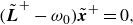(5.4) \begin{align} (\tilde {\boldsymbol{L}}^+-\omega _0) \tilde {\boldsymbol{x}}^{+}=0, \end{align}

where $\tilde {\boldsymbol{L}}^+$ is the adjoint operator of $\tilde {\boldsymbol{L}}$ . By taking the inner product of the first-order equation with $\tilde {\boldsymbol{x}}^{+}$ , we obtain

(5.5) \begin{align} \langle \tilde {\boldsymbol{x}}^{+}, \; (\tilde {\boldsymbol{L}}-\omega _0) \tilde {\boldsymbol{x}}^{(1)}\rangle =\langle \tilde {\boldsymbol{x}}^{+}, \; \boldsymbol{G}(\omega _1, \tilde {\boldsymbol{x}}^{(0)}) \rangle. \end{align}

We then use integration by parts along with (5.4) to obtain

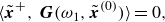(5.6) \begin{align} \langle \tilde {\boldsymbol{x}}^{+}, \; \boldsymbol{G}(\omega _1, \tilde {\boldsymbol{x}}^{(0)}) \rangle =0, \end{align}

which represents the solvability condition for $\omega _1$ .

The leading-order eigenvalue problem can be discretised using a spectral collocation method, resulting in a matrix eigenvalue problem. By employing a sufficiently large number of grid points, we can obtain a reliable estimate of the eigenvalue spectrum for the operator. Since we are mostly concerned to know if the solution is stable or not, our focus lies on identifying the eigenvalue with the largest real part and its corresponding eigenfunction.

Having obtained the numerical solution to the leading-order problem, (5.6) can also be readily solved using a similar spectral collocation method. The quantity $\omega _1$ represents the difference in growth rates between the viscoelastic and Newtonian fluids. However, our main concern is to determine if the real part of $\omega =\omega _0+{De}\, \omega _1$ is positive or negative. Given our assumption that ${De}\ll 1$ , $\omega _1$ can only make a significant difference in determining if the solution is stable or not for the values of the parameters for which the real part of $\omega _0$ is close to zero. Hence, if the real part of $\omega _1$ is positive, then elastic effects act to make the flow more unstable or less stable than the Newtonian flow. We denote the critical draw ratio derived from the leading-order eigenvalue problem as $D_{0c}$ , which signifies the onset of instability in the case of a Newtonian fluid. By analysing the magnitude of $\omega _1$ at $D_{0c}$ , we can determine whether elasticity stabilises or destabilises the drawing process.

Figure 8. (a) $Real(\omega _0)$ versus draw ratio $D$ for various values of the Reynolds number $Re$ . (b) The elastic contribution to the growth rate $Real(\omega _1)$ versus $D$ for various $Re$ . Other parameters are ${Ca}=2,\ \phi =0.5,\ \alpha =0,\ \beta =0$ . For each curve, there is a value of $D$ marked by a black circle at which $Real(\omega _0)=0$ , below which (solid curve) the Newtonian flow is stable ( $Real(\omega _0)\lt 0$ ), above which (dashed curve) it is unstable ( $Real(\omega _0)\gt 0$ ). If $Real(\omega _0+{De}\, \omega _1)=Real(\omega _0)+{De}\, Real(\omega _1)\gt 0$ , the draw process is unstable.

In figure 8(a), curves of the growth rates $Real(\omega _0)$ for Newtonian fluids are shown for different values of Reynolds number $Re$ . For each Reynolds number, the critical draw ratio $D_{0c}$ is at the point of intersection of the curve with the line $Real(\omega _0)=0$ (black circle), the curve is solid for $Real(\omega _0)\lt 0$ (stable) and dashed for $Real(\omega _0)\gt 0$ (unstable). Similarly, in figure 8(b) we plot $Real(\omega _1)$ , which measures how elasticity affects the growth rate, versus the draw ratio D. Since $De\ll 1$ , the most important value of $Real(\omega _1)$ corresponds to the draw ratio $D_{0c}$ at which $Real(\omega _0)=0$ . This is marked as a solid black circle in figure 8(b). In figure 8(b) the solid curve corresponds to values of D for which the zero- $De$ flow is stable ( $Real(\omega _0)\lt 0$ ) and the dashed curve corresponds to values of D for which the zero- $De$ flow is unstable ( $Real(\omega _0)\gt 0$ ). At the critical draw ratio $D_{0c}$ for the zero- $De$ flow (corresponding to the black circles in figure 8 a,b), we see that $Real(\omega _1)$ is positive in the cases of $Re=0$ and $Re=0.01$ , indicating that elastic effects destabilise the drawing process. Conversely, when $Re=0.02,\ 0.05$ and 0.1, elastic effects stabilise the process, since $Real(\omega _1)\lt 0$ .

Figure 9. Plots of $Real(\omega _0)$ versus draw ratio D for various values of the capillary number $Ca$ for (a)  $Re=0$ and (c) $Re=0.01$ . The elastic contribution to growth rate $Real(\omega _1)$ versus D for various $Ca$ for (b) $Re=0$ and (d) $Re=0.01$ . Other parameters are $\phi =0.5,\ \alpha =0,\ \beta =0$ . For each curve, there is a value of D marked by a black circle at which $Real(\omega _0)=0$ , below which (solid curve) the Newtonian flow is stable ( $Real(\omega _0)\lt 0$ ), above which (dashed curve) it is unstable ( $Real(\omega _0)\gt 0$ ). If $Real(\omega _0+{De}\, \omega _1)=Real(\omega _0)+{De}\, Real(\omega _1)\gt 0$ , the draw process is unstable.

Similar plots are shown in figure 9 for fixed $Re$ and different values of the capillary number $Ca$ . Figures 9(a) and 9(b) correspond to $Re=0$ , while figures 9(c) and 9(d) correspond to $Re=0.01$ . Figure 9(b) reveals that elastic effects consistently destabilise the process at $Re=0$ for all $Ca$ considered. On the other hand, figure 9(d) shows that elastic effects destabilise the process if $Ca=2$ , which is consistent with the findings in figure 8. However, for $Ca\geqslant 5$ elastic effects stabilise the drawing process.

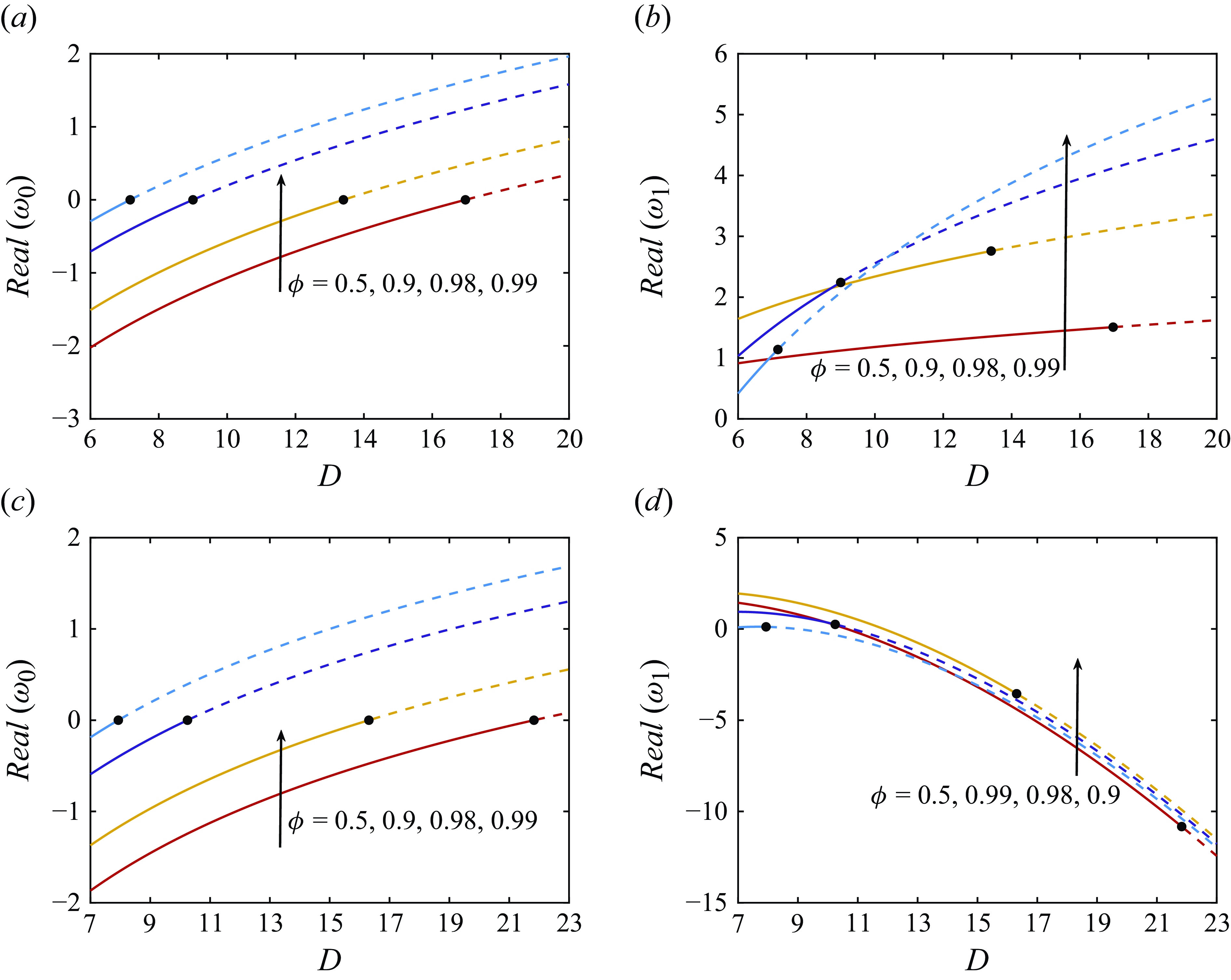
Figure 10. Plots of $Real(\omega _0)$ versus draw ratio D for various values of $\phi$ for (a) $Re=0$ and (c) $Re=0.1$ . The elastic contribution to growth rate $Real(\omega _1)$ versus D for various $\phi$ with (b) $Re=0$ and (d) $Re=0.1$ . Other parameters are $Ca=2,\ \alpha =0,\ \beta =0$ . For each curve, there is a value of D marked by a black circle at which $Real(\omega _0)=0$ , below which (solid curve) the Newtonian flow is stable ( $Real(\omega _0)\lt 0$ ), above which (dashed curve) it is unstable ( $Real(\omega _0)\gt 0$ ). If $Real(\omega _0+{De}\, \omega _1)=Real(\omega _0)+{De}\, Real(\omega _1)\gt 0$ , the draw process is unstable.

In figures 10(a) and 10(c), the growth rates $Real(\omega _0)$ for Newtonian fluids are shown with different inlet hole sizes, for $Re=0$ and $Re=0.1$ , respectively. Again, the critical draw ratios for Newtonian fluids, corresponding to different $\phi$ , are observed at the intersections of the curves with the line $Real(\omega _0)=0$ (black circles), with the solid and dashed portions of the curves denoting stability/instability of the zero- $De$ flow. Furthermore, the influence of inlet hole size on $Real(\omega _1)$ is shown in figures 10(b) and 10(d), for varying values of $\phi$ . We find that $Real(\omega _1)$ is always positive if $Re=0$ , indicating that elasticity destabilises the drawing process. However, when $Re=0.1$ , elastic effects stabilise the process except for large values of $\phi$ sufficiently close to unity, in which case it becomes destabilising.

Figure 11. Plots of $Real(\omega _1)$ versus draw ratio D for various values of the mobility factor $\alpha$ for (a) $Re=0$ and (b) $Re=0.1$ . Other parameters are $\phi =0.5,\ {Ca}=2,\ \beta =0.$ Besides, with these parameters, $Real(\omega _0)$ are plotted against D in figure 8(a).

In figures 11(a) and 11(b), we examine the impact of the mobility factor $\alpha$ on the stability of the drawing process for viscoelastic fluids at $Re=0$ and $Re=0.1$ , respectively. We note that at leading order in $De$ the results for linear stability do not depend on $\alpha$ since this case represents a Newtonian fluid. Therefore, we do not plot $Real(\omega _0)$ versus D, but just note from figure 8(a) that $D_{0c}\approx 17$ for $Re=0$ and $D_{0c}\approx 21.8$ for $Re=0.1$ . With $\alpha =0$ , figure 11 reveals that elastic effects consistently destabilise the process if $Re=0$ , while they stabilise the process if $Re=0.1$ , which is consistent with the findings in previous figures. Additionally, we observe that the process becomes increasingly less stable as $\alpha$ increases, for both $Re=0$ and $Re=0.1$ . When $Re=0.1$ , the elasticity plays a role to stabilise the process for $\alpha \leqslant 0.2$ ; however, it destabilises the process for larger $\alpha$ .

The effect of the polymer concentration, $\beta$ , on $Real(\omega _1)$ is not presented. This is because the role it plays is rather straightforward. As $\beta$ approaches $1$ , the polymer concentration becomes zero, causing the flow to behave like a Newtonian fluid. Consequently, $Real(\omega _1)$ tends to zero when $\beta \to 1$ . In fact as $\beta$ increases, $Real(\omega _1)$ monotonically tends to zero and the effect of elasticity is, hence, reduced.

6. Conclusions

In this paper, we have determined the steady-state behaviour and analysed the stability of the drawing process for an axisymmetric tube composed of a Giesekus fluid. Our analysis takes into account surface tension and inertial effects. We have used asymptotic techniques to obtain a set of one-dimensional equations that describe the flow in the case of weak elastic effects. We have obtained the steady-state profiles and found that, in almost all of the parameter space, elastic effects make the hole close more rapidly than in the zero-Deborah-number case, equivalent to Newtonian fibre drawing. This is counterintuitive in the sense that one would probably naively imagine that the elastic stresses would oppose the inward radial flow induced by the surface tension and hence cause the hole to close more slowly. From our analysis, the stresses are advected by the zero-Deborah-number flow in both axial and radial directions. The advection causes changes in the stresses that will be opposed by elastic effects and hence induces corrections to the second normal stress difference. These second normal stress differences are the key mechanism by which the elasticity affects hole evolution. For almost the whole parameter space, the correction to the second normal stress difference is negative, which induces an additional radially inward flow that causes the hole to close more rapidly than in the Newtonian case. We also showed that there is a small region of the parameter space for which the hole radius at the inlet nozzle is sufficiently close to the outer radius. In this case, the axial advection of stress by the Newtonian flow causes the correction to the second normal stress difference to be large and positive near the inlet nozzle of the device, which induces a strong outward flow. This outward flow near the inlet nozzle dominates the hole closure that occurs over the rest of the device, so that the hole at the take-up point is larger than in the Newtonian case.

In fibre drawing, a reduction of the hole closure due to surface tension effects is, typically, desired. Our results indicate that elastic effects will be detrimental to achieving this goal for tubes that have a moderate hole size at the inlet nozzle of the device. However, for tubes that have a sufficiently large hole size at the inlet nozzle of the device and sufficiently small draw ratio we do indeed obtain the desired effect. Moreover, there is a class of MOFs that have very large air holes and a very small amount of their cross-sectional area occupied by the fluid (Argyros & Pla 2007). These types of MOFs are very heavily affected by surface tension and it therefore seems that elastic effects may be very useful in the fabrication of such fibres.

We also examined the linear stability of the drawing process for weakly viscoelastic materials to determine whether elastic effects act to stabilise or destabilise the drawing process relative to the Newtonian case. We have shown that if inertia is negligible, elastic effects are always destabilising. On the other hand, for non-zero inertia, elastic effects can be stabilising if the capillary number is sufficiently large, or if the initial hole size is sufficiently small. The main goal in manufacturing is to suppress hole closure and our steady-state results showed that this only occurs for large input hole sizes. Unfortunately, for large input hole sizes elastic effects act to destabilise the flow. However, there is a trade-off between Reynolds number and hole size in determining stability, and inertia acts to stabilise. Elastic effects also act to stabilise the flow for small values of $\alpha$ indicating that Oldroyd-B fluids are more stable than Giesekus fluids. This will be of interest when selecting materials for drawing. The instability mechanism for Newtonian fluids has been thoroughly examined by Bechert & Scheid (2017) in the context of solid threads and by Wylie et al. (2023) for threads with internal holes. They proposed that this instability arises from a process where a slight increase in the cross-sectional area near the exit results in heightened tension in the thread. This increased tension is transmitted upstream, leading to a more rapid thinning of the thread near the entrance. Consequently, this thinned section of the thread is advected towards the exit, resulting in a reduction of the cross-sectional area at that location. This represents a half-cycle of the instability. The instability mechanism is outlined in a schematic presented by Bechert & Scheid (2017). For Newtonian fluids they showed that inertia reduces the transmission of the tension upstream and hence weakens the instability mechanism. In this study, for a viscoelastic fluid, the force transmission is affected by inertia, surface tension and elastic effects and it is challenging to fully understand the mechanism by which these forces determine the stability.

When drawing optical fibres, the draw ratio D is typically chosen to be as large as possible. In this case elastic effects enhance hole closure, which is not typically desirable in manufacturing settings. But for extrusion flows which typically have moderate D, elastic effects can suppress hole closure for tubes with large air holes. Extrusion flows typically have very low $Re$ , so elastic effects will act to destabilise. But in extrusion flows draw ratios typically used in manufacturing settings are sufficiently small that the zero- $De$ flow will be strongly stable and so the destabilising issues associated with elastic effects will not be a concern. Therefore, generally speaking, elastic effects will be detrimental to the manufacturing goals for fibre drawing, but may be beneficial to the manufacturing goals for extrusion flows with large air holes.

In practical applications, thermal effects can play a significant role, as rheological properties often change considerably with temperature. Several models that account for these thermal effects have been proposed in the literature. For instance, Gupta & Chokshi (2018) and Xu & Jiang (2022) directly treat the solvent viscosity, polymer viscosity and relaxation time as functions of temperature. Joo et al. (2002) adopted a non-isothermal version of the Giesekus model, derived using the pseudo-time method applied to the isothermal model. In fact, it is relatively straightforward to apply the techniques we have developed in this paper to investigate such models. However, doing so falls outside the scope of this current work.