Microstructure and deformation in suspensions of soft microswimmers

Abstract

In recent years, various unique properties of microswimmer suspensions have been revealed. Some microswimmers are deformable; however, the influence of the swimmer’s deformability has been overlooked. The present study examined the impact of soft microswimmers’ membrane deformations in a mono-dispersed dense suspension on microstructure formation. Due to the small size of the microswimmers, the flow field is described by the Stokes equation. The soft microswimmer was modelled as a capsule with a two-dimensional hyperelastic membrane enclosing a Newtonian fluid that is driven by propulsion torques distributed slightly above the membrane surface. Changes to the torque distribution caused the soft swimmer to exhibit different swimming modes as a pusher or puller. Similar to rigid squirmers, soft swimmers displayed self-organised local clusters in the suspension. Membrane deformation changed the mutual interference among swimmers in the cluster, bringing the interactions closer together than those of rigid squirmers. Especially among soft pushers, rotational diffusion due to hydrodynamic interference was reduced and the swimming trajectory became relatively straight. As a result, polar order was less likely to form, especially in regions of high $Ca$. On the other hand, pullers showed strong interactions due to retraction flow and an increase in mean membrane tension. For pushers (pullers), the rear (side) interaction produced the greatest change in tension. These findings are expected to be useful for effort to understand the propulsion mechanisms of medical and industrial soft microrobots, as well as the biological responses of microorganisms induced by mechanical stimuli.

1. Introduction

Suspensions consisting of particles dispersed in a liquid are evident throughout nature and daily life; they are critical for industrial purposes in various fields and environments. Theoretical and experimental studies have been conducted in attempts to better understand and predict the rheological properties, microstructures and transport phenomena in such multiphase flows. In early theoretical studies, the analysis was limited to a dilute regime with a low Reynolds number. Where single- or two-particle interactions are dominant, the macroscopic suspension properties are commonly determined by the expansion of the volume fraction. For example, Einstein (1906) derived the effective viscosity of a dilute suspension of non-Brownian spheres, resulting in the first-order term of the viscosity as 2.5 $\phi$ , where $\phi$ is the volume fraction. Batchelor (1970) derived a stress system of force-free particle suspensions by introducing the particle stress tensor, and Batchelor & Green (1972) calculated the bulk stress in the second-order term of the volume fraction from the two-body particle interactions. Particle deformability leads to deviation from the streamline during two-body interactions (Lac, Morel & Barthes-Biesel 2007). The shear-induced self-diffusion of droplets and red blood cells in the semi-dilute regime has been quantified from two-body hydrodynamic interactions (Loewenberg & Hinch 1997; Omori et al. 2013). The theory of dilute suspensions is well organised, and there are several relevant review articles (Brenner 1974; Jeffery & Acrivos 1976; Russel 1980; Davis & Acrivos 1985).

For suspensions with higher volume fractions, many-body interactions play a role. With respect to concentrated suspensions of rigid particles, it is necessary to accurately determine the lubrication forces acting between particles in near contact. Moreover, particle interactions at an infinite distance may be considered due to the long-range nature of Stokes flow. Stokesian dynamics that accurately compute both the short-range lubrication forces and long-range particle interactions has been developed and reviewed by Brady & Bossis (1988). For example, the shear-induced diffusion of Brownian particles in concentrated suspensions (Bossis & Brady 1987) and the rheological properties of concentrated suspensions of spheres (Brady & Bossis 1985) have been analysed using Stokesian dynamics. In a highly concentrated state, jamming phenomena can be observed at a critical volume fraction ( ${\approx}0.64$ for non-Brownian particles, Mari et al. (2014)), with the viscosity rapidly increasing when the volume fraction exceeds the critical threshold. Krieger & Dougherty (1959) derived an empirical equation of the viscosity from the dilute to the jamming regime. Blanc et al. (2013) reported the shear-induced anisotropic microstructure of non-Brownian particles in dense suspensions. Reviews about the rheology and microstructures of dense suspensions of rigid particles are presented in works by Ness, Seto & Mari (2022) and Guazzelli & Pouliquen (2018).

The suspension dynamics of microswimmers has received considerable interest in recent years, particularly in the fields of active fluids and active matter (Zöttl & Stark 2016; Saintillan 2018). The squirmer model, developed by Lighthill (1952) and Blake (1971), is widely used to describe the fluid dynamics of microswimmers (Ishikawa 2024). By varying the surface velocity distribution of the squirmer, it is possible to represent a range of velocity fields around the particle. This leads to various hydrodynamic interactions between the self-propelled particles, as reported in a number of interesting phenomena. Ishikawa, Simmonds & Pedley (2006) successfully introduced the squirmer model in analyses of the two-body interference problem. The model was extended to a Stokesian dynamics framework for concentrated monolayer suspensions (Ishikawa and Pedley 2008); they demonstrated that clustering and collective swimming of non-bottom-heavy strong pullers occurs, whereas for the weak puller and weak pusher, a global coherent polar order was formed. Similar results have been demonstrated in the fully three-dimensional suspension (Ishikawa et al. 2008), where the global coherent structure of weak pullers was the result of short-range interactions between squirmers. The aggregation of pusher-type swimmers generates strong elongational flows, which may lead to instabilities in the particle structure (Ishikawa, Dang & Lauga 2022). Hydrodynamic interactions of ellipsoid squirmers were analysed using a boundary element method (Kyoya et al. 2015), and it was concluded that the nearest-neighbour two-body interference leads to collective swimming of the squirmers. The importance of the near-field interaction has also been reported by Yoshinaga & Liverpool (2008). After application of a lubrication force, a phase change is observed, whereby the gel-like cell aggregation transforms into a polar order with an aligned swimming direction. This is achieved by alteration of the swimming mode. The formation of a neutral-type coordinated swimming pattern is not observed in the absence of short-range interactions.

Some microswimmers are deformable, as evidenced by the behaviour of a ciliate in close proximity to a wall (Ishikawa & Kikuchi 2018). For example, the ciliate Paramecium exhibits a physiological response, termed the avoiding reaction, when its cell membrane is mechanically stimulated (Jennings 1904). The cell initially exhibits backward swimming motion, followed by rotational movement about its posterior end, before resuming normal forward locomotion. Membrane deformation and tension are important for understanding this microbial behaviour. Swimmer deformability may also influence short-range interactions. Menzel & Ohta (2012) developed a model of a soft self-propelled particle capable of deformation due to local pairwise interactions; they demonstrated that deformation could facilitate alignment effects between colliding particles, resulting in a rapid transition to a global ordered state with increasing deformability. A ring polymer model (Wen et al. 2022) and migrating cell model on a substrate (Coburn et al. 2013; Löber et al. 2015) have been proposed. These models showed that a swimmer’s elastic behaviour alters migration and interparticle collisions, leading to changes in mean cluster diameter and degree of orientational order; notably, these models do not consider hydrodynamic interactions. Matsui, Omori & Ishikawa (2020a ) analysed the impact of elastohydrodynamic interactions of capsule-type microswimmers using a boundary element--finite-element coupling method. The ciliary flow near the cell membrane was modelled as an external torque, in accordance with Ishikawa et al. (2016), utilising a two-dimensional hyperelastic constitutive law. Particle deformation reduces orbital displacement during two-body interference, suggesting that the self-diffusion of self-propelled particles could be suppressed by their deformability. Under shear flow, orientation in the vorticity direction has been observed (Matsui, Omori & Ishikawa 2020b ), which was not observed for the rigid squirmer. Although these findings demonstrate the importance of particle deformation under hydrodynamic interaction, they are limited to the dilute regime. Thus, the impact of deformation in the dense regime includingthe effect of three or more body interferences remains unclear.

The objective of this study was to investigate the hydrodynamic interactions of soft microswimmers in a dense suspension. A hyperelastic capsule with a thrust torque was utilised as a soft swimmer (Matsui et al. 2020a , b ). In this paper the basic equations and numerical method are presented in § 2. The effects of the membrane deformability and the swimming mode on the microstructure formation are investigated in § 3. The membrane tension induced by cell--cell interactions is discussed in § 4, and a summary of our findings and concluding remarks are presented in § 5.

2. Basic equations and numerical methods

This section outlines the fundamental equations and the numerical model used in the present study. A torque-induced soft microswimmer developed by Ishikawa et al. (2016) was utilised. The methodology is briefly outlined here. For further details, please refer to Ishikawa et al. (2016) and Matsui et al. (2020a , b ).

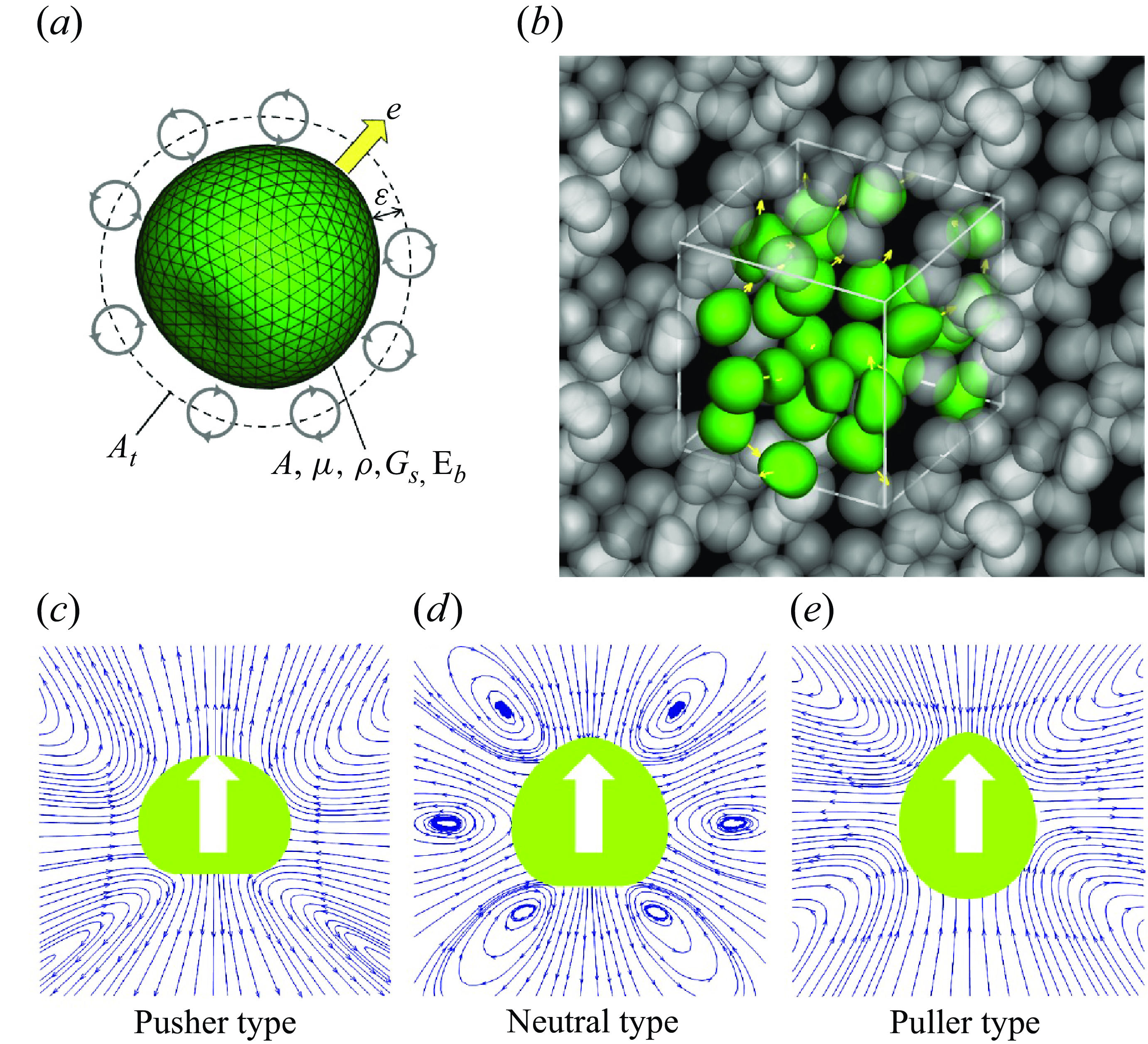
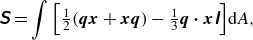
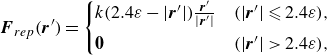
Figure 1. Problem settings and the soft microswimmer model. (a) Soft swimmer is modelled by a capsule with a hyperelastic thin membrane with the shear elastic modulus $G_s$ and the bending modulus $E_b$ . Propulsion torque is generated on the torque surface $A_t$ (slightly above the membrane surface $A$ ). (b–d) Flow fields created by the soft swimmer. In this study, $\beta$ is set to −0.9 for pushers, 0 for neutral swimmers and 0.9 for pullers. The white arrow indicates the swimming direction and blue arrow is the streamline. (e) Here 27 swimmers (depicted by green in the figure) are freely suspended in the computational unit and the triply periodic boundary condition is applied to the domain.

2.1. Soft microswimmer and problem settings

Consider microswimmers with a radius of $a$ swimming freely in an incompressible Newtonian liquid with a viscosity of $\mu$ and a density of $\rho$ . Due to the small size of the microswimmers, the particle Reynolds number is much smaller than unity, as such the inertial effect of the fluid flow can be neglected. The flow field is then governed by the Stokes equation. The microswimmer consists of a two-dimensional hyperelastic thin membrane enclosing a Newtonian liquid with the same viscosity and density as the external liquid. A torque swimmer model (Ishikawa et al. 2016) was originally developed to represent a ciliate. The model expresses the thrust force at the tip of a cilium and the reaction force at the root of the cilium as a torque on the surface $A_t$ at a distance of $\varepsilon$ from the membrane (cf. figure 1 a). The magnitude of the propulsive torque density per unit area in the reference state $L_r$ is given by

(2.1) \begin{align} L_r = L_0 + \kappa \left ( \theta - \frac {\pi }{2} \right ), \end{align}

where $\kappa$ determines the torque strength of the asymmetry and $\theta$ is the polar angle with respect to the orientation vector $\boldsymbol {e}$ .

The torque density $L_0$ is defined as the value at which the swimming speed of the rigid body is equal to $U_0$ . The swimmer in the reference state satisfies the torque-free condition on the overall torque surface due to the axisymmetric torque distribution. The instantaneous torque density per unit area in the deformed state $L$ is given by

(2.2) \begin{align} L = L_r\frac { \mathrm{d} \it A_{t,r}}{ \mathrm{d} \it A_t} , \end{align}

where $ \mathrm{d}\it A_{t,r}$ and $ \mathrm{d} \it A_t$ are the local torque surface area in the reference and deformed states, respectively. This correction means that the number of cilia does not change with deformation. The propulsive torque in vector form is given by $\boldsymbol {L} = L\boldsymbol {n} \times \boldsymbol {t}$ , where $\boldsymbol {n}$ is the unit outward normal vector and $\boldsymbol {t}$ is the unit tangential vector inthe $\theta$ direction on the membrane surface. The soft swimmer is deformed from its reference shape by the propulsive torque distribution, resulting in a swimming-induced stresslet $\unicode{x1D64E}$ (Matsui et al. 2020b ):

(2.3) \begin{align} \unicode{x1D64E} = \int { \left [ \tfrac {1}{2}(\boldsymbol {q}\boldsymbol {x} + \boldsymbol {x}\boldsymbol {q}) - \tfrac {1}{3}\boldsymbol {q} \boldsymbol{\cdot} \boldsymbol {x}\unicode{x1D644} \right ]} \mathrm{d}\kern1pt \textit{A}, \end{align}

where $\boldsymbol {q}$ is the traction at the point $\boldsymbol {x}$ on the membrane $A$ and $\unicode{x1D644}$ is the identity matrix. By changing $\kappa$ in (2.1), various swimming modes can be expressed as puller, neutral and pusher types (figure 1 b–d), respectively. In the rigid squirmer (Blake 1971), the swimming mode is often expressed by positive and negative values of the second mode $\beta$ :

(2.4) \begin{align} v_{\theta } = U_0 \left ( \tfrac {3}{2}\sin \theta + \tfrac {3}{2}\beta \sin \theta \cos \theta \right ). \end{align}

Here $v_{\theta }$ is the squirming velocity on the squirmer surface. In this study the swimming mode is also defined using $\beta$ obtained from $\unicode{x1D64E}$ with reference to the rigid squirmer model, i.e.

(2.5) \begin{align} {S}_{ee}=4\pi \mu a^2\beta , \end{align}

where ${S}_{ee}$ is the stresslet component in the swimming direction.Here $\kappa$ is adjusted to ensure that, under the same $\beta$ , the stresslet produced by the rigid squirmer and the soft swimmer are the same. The correspondences between $\kappa$ and $\beta$ are almost linear as shown in figure 2. In this study, $\beta$ is set to −0.9 for pushers, 0 for neutral swimmers and 0.9 for pullers.

Figure 2. The relationship between the asymmetry of torque strength $\kappa$ , the stresslet component in the swimming direction ${S}_{ee}$ and the swimming mode $\beta$ of the soft swimmer with each $Ca$ . Here $Ca$ is the ratio between the viscous force due to swimming and the elastic force of the membrane defined by (2.22).

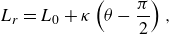
Assuming an infinite suspension, triply periodic boundary conditions were applied, as shown in figure 1(e). Twenty-seven soft swimmers with random orientations were placed in random initial positions in the computational unit domain. The volume fraction $\phi$ was varied from 0.03 to 0.2 by changing the domain size. According to the scaling by Batchelor & Green (1972), the frequency of $n$ -body interference is proportional to $\phi ^n$ . Thus, for $\phi = 0.2$ , the influence of three-body interference is expected to be 20 % of two-body interference.

2.2. Membrane mechanics

The coupling of thin-shell theory of capsules with fluid mech anics has been developed by the work of Barthès-Biesel, Pozrikidis and their co-workers. Therefore, we briefly explain the outline of thin-shell theory in the main text. For further details, please refer to Barthès-Biesel et al. (2002), Lac et al. (2004), Walter et al. (2010) and Pozrikidis (2010). The swimmer’s membrane is modelled as a hyperelastic thin material. A material point of the membrane in the reference state is represented by $\boldsymbol {X}$ ; $\boldsymbol {x}(\boldsymbol {X},t)$ expresses the deformed state. Using a surface deformation gradient tensor $\unicode{x1D641}_s$ , reference and deformed states have the following relationship (Pozrikidis 2010):

(2.6) \begin{align} \boldsymbol {dx} = \unicode{x1D641}_s \boldsymbol{\cdot} \boldsymbol {d \it X}, \end{align}

where $\unicode{x1D641}_s = \partial \boldsymbol{x}/\partial \boldsymbol{X}$ . The Green--Lagrange strain tensor $\unicode{x1D640}$ describing local deformation of the membrane is as follows:

(2.7) \begin{align} \unicode{x1D640} = \tfrac {1}{2} \big( \unicode{x1D641}_s^T \unicode{x1D641}_s - \unicode{x1D644} \big). \end{align}

The first and second invariants of the strain tensor are given by the principal extension ratios $\lambda _1$ and $\lambda _2$ as

(2.8) \begin{align} I_1= \lambda _1^2 + \lambda _2^2 -2 \end{align}

and

(2.9) \begin{align} I_2 = \lambda _1^2 \lambda _2^2 -1 = J^2_s - 1 , \end{align}

where $J_s$ = det( $\unicode{x1D641}_s)=\lambda _1 \lambda _2$ is the Jacobian expressing the area dilatation. Because the membrane is modelled as a two-dimensional hyperelastic material, the Cauchy tension $\unicode{x1D64F}_{\boldsymbol{s}}$ and the strain energy function $w_s(I_1, I_2)$ have the following relationship:

(2.10) \begin{align} \unicode{x1D64F}_{\boldsymbol {s}} &= \frac {1}{J_s} \unicode{x1D641}_s \boldsymbol{\cdot} \frac {\partial w_s}{\partial \unicode{x1D640}} \boldsymbol{\cdot} \unicode{x1D641}^T_s . \end{align}

In order to express strain hardening behaviour and the incompressible areal dilatation of a biological membrane, we utilise the constitutive law proposed by Skalak et al. (1973). The strain energy function of the Skalak model is given by

(2.11) \begin{align} w_s = \frac {G_s}{4} \big( I^2_1 + 2I_1 - 2I_2 + CI^2_2 \big) , \end{align}

where $G_s$ is the surface shear elastic modulus and $C$ is the non-dimensional areal dilatation constant. The Poisson ratio of the Skalak law is $\nu _s = C/(1+C)$ . The value of $C$ is set to 10 with reference to the erythrocyte model (Omori et al. 2013).

The bending energy of the biological membrane, derived by Helfrich (1973), is

(2.12) \begin{align} w_b = \frac {E_b}{2}\int \left ( 2H-c_0 \right ) \mathrm{d}\kern1pt \textit{A}, \end{align}

where $H$ is the mean curvature of the membrane, $c_0$ is the spontaneous curvature and $E_b$ is the bending modulus. By assuming a symmetric membrane property (i.e. $c_0 = 0$ ), the energy can be converted to the force density $\boldsymbol {q}_b$ as (Matsui et al. 2020a )

(2.13) \begin{align} \boldsymbol {q}_b = -2E_b\big[\Delta _sH + 2H(H^2 - K)\big]\boldsymbol {n}, \end{align}

where $\Delta _s$ is the Laplace--Beltrami operator and $K$ is the Gaussian curvature on the membrane surface.

2.3. Fluid mechanics

Due to the small size of the swimmer, the inertial effect of fluid flow is negligible. Therefore, the flow field is governed by the Stokes equation, and the fluid velocity $\boldsymbol {v}$ at an arbitrary point $\boldsymbol {y}$ is given by the boundary integral equation (Pozrikidis 1992) as

(2.14) \begin{align} \boldsymbol {v}(\boldsymbol {y}) = - \frac {1}{8\pi \mu }\sum _i^N \left [ \int _{A} \unicode{x1D645}(\boldsymbol {x},\boldsymbol {y}) \boldsymbol{\cdot} \boldsymbol {q}(\boldsymbol {x}) \mathrm{d}\kern1pt \textit{A}^i + \int _{A_{t}} \unicode{x1D64D}(\boldsymbol {x},\boldsymbol {y}) \boldsymbol{\cdot} \boldsymbol {L}(\boldsymbol {x}) \mathrm{d} \kern1pt A^i_t \right ] , \end{align}

where $N$ is the number of microswimmers in the fluid domain. Here, $\unicode{x1D645}$ and $\unicode{x1D64D}$ are the Green’s function of the Stokeslet and torque in the triply periodic boundaries, respectively (Beenakker 1986):

(2.15) \begin{align} \unicode{x1D645} = \unicode{x1D645}^{1} + \unicode{x1D645}^{\kern1pt 2}, \end{align}

(2.16) \begin{align} \unicode{x1D64D} = \unicode{x1D64D}^{1} + \unicode{x1D64D}^{\kern1pt 2}, \end{align}

(2.17) \begin{align} \begin{bmatrix} {J}^{1}_{i j} \\[4pt] {J}^{\kern1pt 2}_{i j} \end{bmatrix} = (\delta _{i j} \nabla ^{2}-\nabla _{i} \nabla _{j}) \begin{bmatrix} r\:\mathrm {erfc}(\xi r) \\[4pt] r\:\mathrm {erf}(\xi r) \end{bmatrix}, \end{align}

(2.18) \begin{align} \begin{bmatrix} {R}^{1}_{i j} \\[4pt] {R}^{\kern1pt 2}_{i j} \end{bmatrix} = \tfrac {1}{4} \varepsilon _{l k j}(\nabla _{k} - \nabla _{l}) \begin{bmatrix} {J}^{1}_{i l} \\[4pt] {J}^{\kern1pt 2}_{i k} \end{bmatrix}, \end{align}

where $\boldsymbol {\delta }$ is the Kronecker delta, $\boldsymbol {\varepsilon }$ is the Levi-Civita epsilon and $\xi$ is an arbitrary positive constant with dimensions of inverse length for controlling the convergence rate of the error function and complementary error function. For a simple cubic lattice, the optimal value of the convergence rate that minimises the computational cost for the periodic expansion is given by $\sqrt {\pi }/V^{1/3}$ (Pozrikidis 1992), where $V$ is the volume of the computational domain. The traction $\boldsymbol {q}$ is given by the stress jump across the thin membrane as

(2.19) \begin{align} \boldsymbol {q}(\boldsymbol {x}) = \left [ \boldsymbol {\sigma }_{out}(\boldsymbol {x}) - \boldsymbol {\sigma }_{in}(\boldsymbol {x}) \right ] \boldsymbol{\cdot} \boldsymbol {n}(\boldsymbol {x}) , \end{align}

where $\boldsymbol {\sigma }_{in}$ and $\boldsymbol {\sigma }_{out}$ represent viscous stress on the surface from inside and outside of the membrane, respectively.

2.4. Numerical methods

In this section we briefly explain the numerical method. The swimmer’s membrane and torque surface are respectively discretised by 1280 triangular elements, with 642 vertices, as shown in figure 1(a). Each material point is tracked in terms of its associated Lagrangian, and the strain at any time $t$ is determined. The tension is calculated based on Skalak’s constitutive law, and the load $\boldsymbol {q}$ acting on the membrane is obtained from the weak-form equilibrium equation, given as

(2.20) \begin{align} \int _A \hat {\boldsymbol {u}} \boldsymbol{\cdot} \boldsymbol {q}_s \mathrm{d}\kern1pt \textit{A} = \int _A \boldsymbol{\hat{\varepsilon }} : \unicode{x1D64F}_s \, \mathrm{d}\kern1pt \textit{A}, \end{align}

where $\hat {\boldsymbol {u}}$ is the virtual displacement and ${\boldsymbol{\hat{\varepsilon}}} = \ ({1}/{2})(\nabla _s \hat {\boldsymbol {u}} + \nabla _s \hat {\boldsymbol {u}}^T)$ is the virtual strain. The above equation is solved using a finite-element method (Walter et al. 2010) with respect to unknown $\boldsymbol {q}_s$ . Assuming a linear sum of the loads due to in-plane deformation and the loads due to bending deformation, the load on the membrane surface is determined by $\boldsymbol {q} = \boldsymbol {q}_s + \boldsymbol {q}_b$ . When $\boldsymbol {q}$ is obtained, it is substituted into the boundary integral equation; the velocity $\boldsymbol {v}$ is computed using a Gaussian quadrature method with six numerical integration points in each element. A material point on the torque surface $\boldsymbol {x}_t$ is given by $\boldsymbol {x}_t = \boldsymbol {x}+\varepsilon \boldsymbol {n}(\boldsymbol {x})$ , and the flow due to the torque $\boldsymbol {L}$ is calculated in the same manner. In order to coincide with the half-length of the cilia, $\varepsilon$ is set to $0.05a$ , where $a$ is the radius of the swimmer. Assuming a no-slip boundary at the membrane, $\mathrm{d}\kern1pt \boldsymbol{x}/ \mathrm{d}\it t = \boldsymbol {v}$ , the material point $\boldsymbol {x}$ is updated by a second-order Runge–Kutta method. The above cycles are iteratively calculated to simulate hydrodynamic interactions in the suspension.

A multipole expansion technique is introduced to accelerate the computation (Pozrikidis 1992). Depending on the distance between swimmers’ centres, three regions corresponding to (i) short-range, (ii) middle-range and (iii) long-range interactions are considered in the calculation. For the short-range interaction ( $r \leqslant r_{sm}$ ), the boundary integral equations are numerically integrated using all 1280 elements. In the middle-range interaction ( $r_{sm} \lt r \leqslant r_{ml}$ ), a coarse-grained 20 triangle mesh is used for the calculation; the point stresslet and torque defined at each mass centre are utilised for long-range interactions ( $r \gt r_{ml}$ ). Threshold values $r_{sm} = 4a$ and $r_{ml} =V^{1/3}$ were set to preserve computational accuracy.

The overlap between meshes becomes problematic when the swimmers are very close together (i.e. of the order of the mesh size). Assuming repulsion between cilia, the repulsive force at very short distances is defined as

(2.21) \begin{align} \boldsymbol {F}_{rep}(\boldsymbol {r}^{\prime}) = \begin{cases} k (2.4\varepsilon - |\boldsymbol {r}^{\prime}|) \frac {\boldsymbol {r}^{\prime}}{|\boldsymbol {r}^{\prime}|} & (|\boldsymbol {r}^{\prime}| \leqslant 2.4\varepsilon ), \\[4pt] \boldsymbol {0} &(|\boldsymbol {r}^{\prime}|\gt 2.4\varepsilon ) , \end{cases} \end{align}

where $\boldsymbol {r}^{\prime}$ is the distance between node points on the torque surface of each swimmer and $k$ represents the magnitude of the repulsion. In this study, $k/\mu U_0 = 500$ was set to be consistent with the ciliary elasticity estimated from the bending stiffness of the cilia (Katoh et al. 2023).

Membrane deformability is normalised by the capillary number $Ca$ :

(2.22) \begin{align} \textit {Ca} = \frac {\mu U_0}{G_s} . \end{align}

This dimensionless number represents the ratio between the viscous force due to swimming and the elastic force of the membrane. All computations were normalised by using the radius $a$ , swimming speed $U_0$ and surface shear elastic modulus $G_s$ . Here $\phi$ was changed by varying the length, whereas the number of swimmers remained fixed at 27.

3. Microstructure

We first show hydrodynamic interactions of puller-type swimmers in figure 3. Swimmers were initially assigned random positions and orientations. Here $\phi$ was set to 0.1 and the capillary number was $Ca = 0.1$ . In the suspension the pullers repeatedly interacted with large deformations, forming small clusters. The trajectories slightly changed during the interaction, as shown in figure 3(b). When the pullers passed each other, they swam in relatively straight lines.

Figure 3. Puller swimmers with $Ca = 0.1$ and $\phi = 0.1$ . (a) Instantaneous snapshot of 27 pullers. Red and blue markers indicate the head and tail points, respectively. (b) Trajectories of 27 swimmers. Red markers indicate each final position of the mass centres.

3.1. Orientational correlations

For a more quantitative analysis, we define self-correlation of the swimming direction from the initial direction as

(3.1) \begin{align} I_{e_0} (t) = \left \langle \boldsymbol {e}_i(t) \boldsymbol{\cdot} \boldsymbol {e}_i(0) \right \rangle _{N} , \end{align}

where the bracket $\left \langle \right \rangle _N$ represents an ensemble average over the number of swimmers $N$ , $\boldsymbol {e}_i$ is the orientation vector of the $i$ th swimmer defined from the posterior and anterior node points. The result is shown in figure 4(c), in which the correlation gradually decreases over time. The relaxation time, corresponding to the time when $I_{e_0} = 1/e$ ( $e$ is Napier’s constant), was approximately estimated in the range of $100 \leqslant tU_0/a \leqslant 200$ for $Ca = 0.03$ , $0.1$ and $0.2$ , whereas that of the rigid puller (Ishikawa & Pedley 2007) was approximately $tU_0/a \simeq 50$ . With respect to soft swimmers, the scattering angles after face-to-face interaction are reduced according to deformability (Matsui et al. 2020a ). Thus, the self-correlation to the initial swimming direction persists for a longer duration as $Ca$ increases, and the swimmers retain their initial orientations longer compared with rigid swimmers. We also investigated the self-correlation of pusher and neutral swimmers (cf. figures 4 a and 4 b). Pusher and neutral soft swimmers tend to have longer relaxation times relative to rigid squirmers, as do pullers.

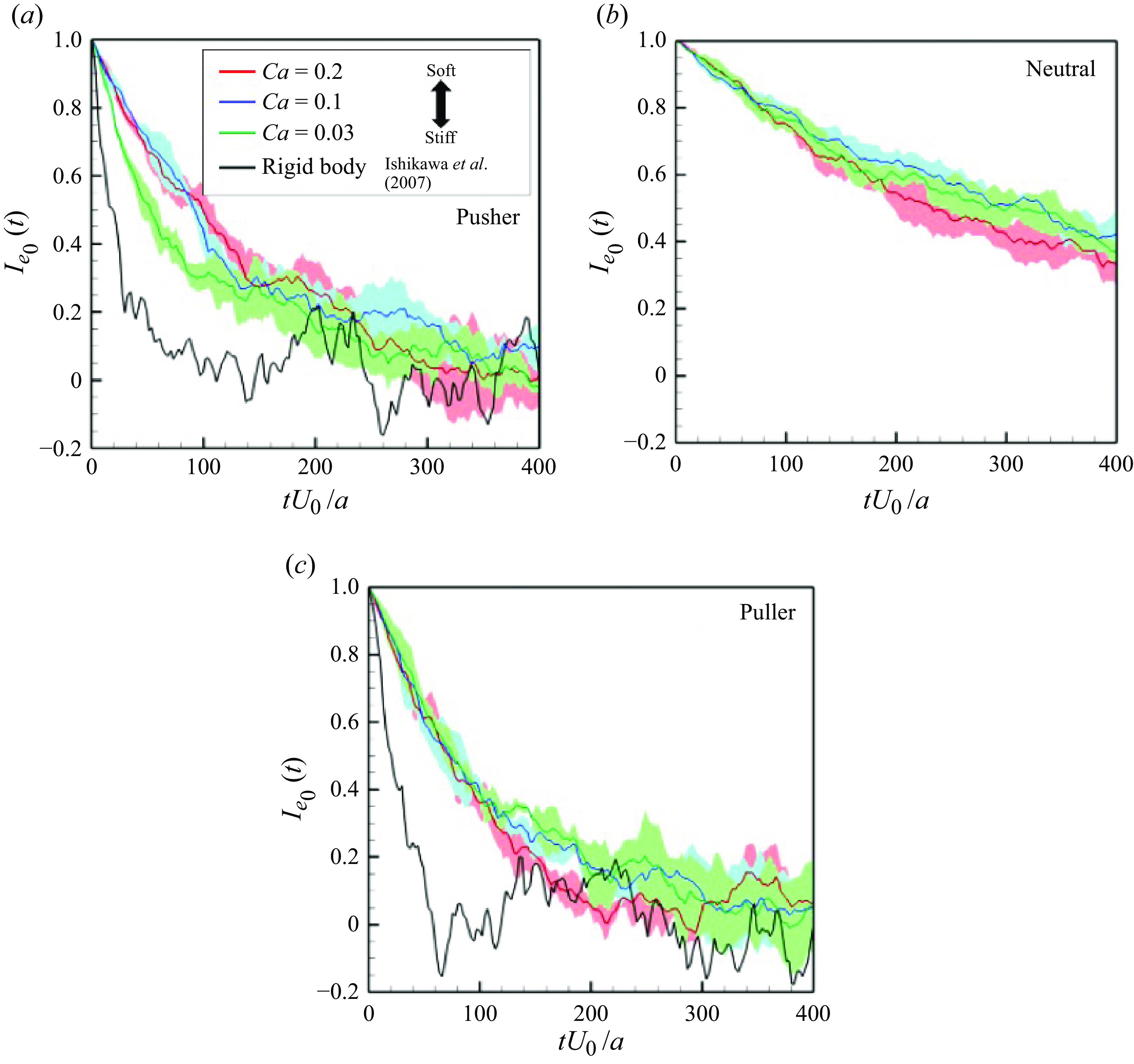
Figure 4. Self-correlations of swimmers’ orientations $I_{e_0}(t) (=\langle \boldsymbol {e}_i(t) \boldsymbol{\cdot} \boldsymbol {e}_i(0) \rangle )$ in the suspension with $\phi = 0.1$ . Here $\boldsymbol {e}_i$ is the swimming direction of the $i$ th swimmer. The coloured lines and area shows the averaged values and standard deviations for the three independent cases throughout the paper. The black lines show the result of rigid squirmmers reported by Ishikawa & Pedley (2007).

In order to investigate the time scale for microstructure development in the suspension, the global order correlation is defined as

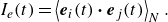(3.2) \begin{align} I_e(t)=\left \langle \boldsymbol {e}_i(t) \boldsymbol{\cdot} \boldsymbol {e}_j(t) \right \rangle _N. \end{align}

To ensure that they would not affect the final structure, two initial conditions were set: (i) an initial polar order and (ii) an initial random configuration. The global correlation of the swimming directions reached a developed state when $tU_0/a \gt 100$ for pushers (cf. figure 5 a) and $tU_0/a \gt 200$ for pullers (cf. figure 5 b). These times were close to the relaxation times of the self-correlation; the converged values of $I_e$ were almost 0 for pushers and 0.2 for pullers. These results suggest that pullers achieve collective swimming, in which the swimmers are more aligned with each other’s swimming direction relative to pushers, similar to the behaviour of rigid squirmers (Ishikawa & Pedley 2007).

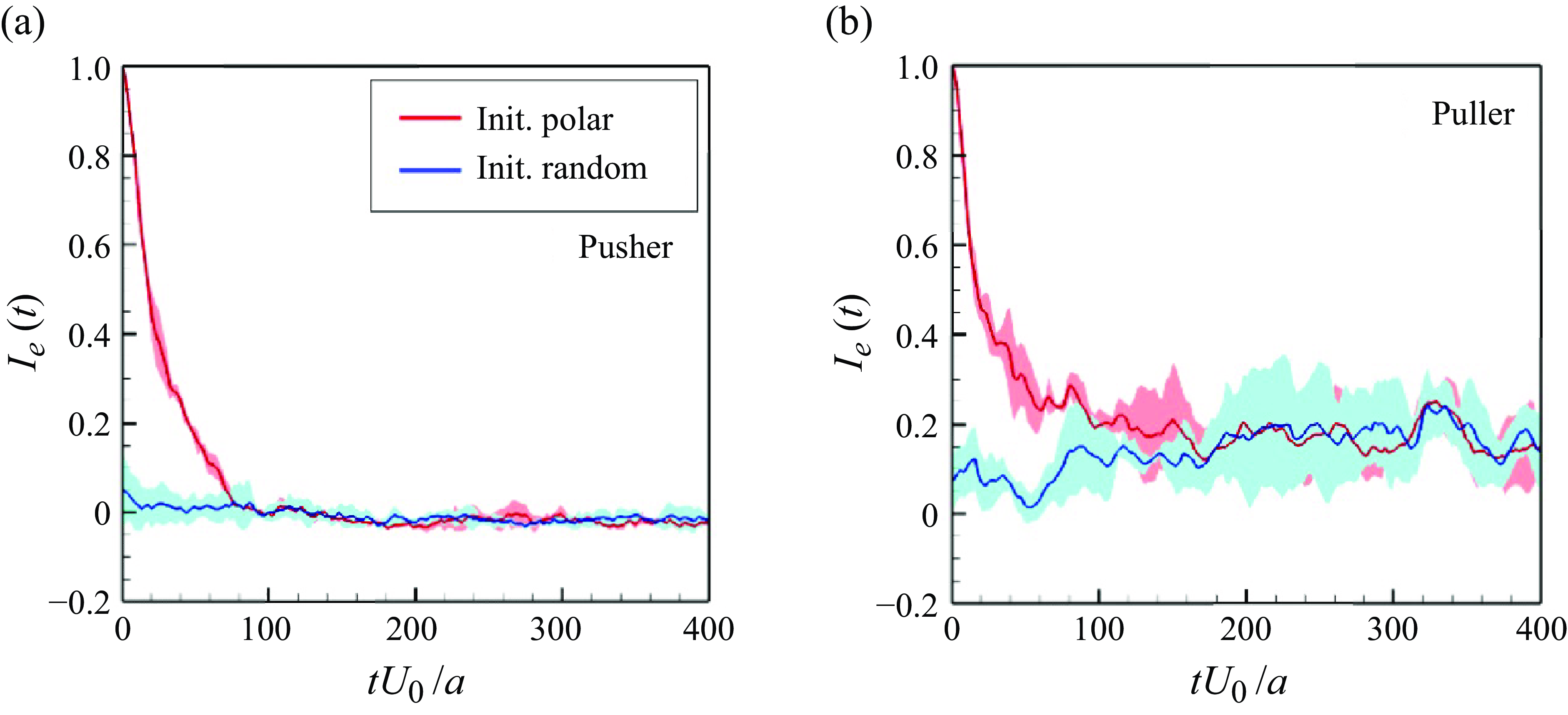
Figure 5. Time change of the global correlation of swimmers’ orientations $Ie(t)(=\langle \boldsymbol {e}_i(t) \boldsymbol{\cdot} \boldsymbol {e}_j(t) \rangle )$ with $\phi = 0.1$ and $Ca = 0.1$ .

Figure 6. Correlations of swimmers’ orientations as a function of relative distance $I_e(t)(=\langle \boldsymbol {e}_i(r_i) \boldsymbol{\cdot} \boldsymbol {e}_j(r_j \rangle )$ with the $\phi = 0.1$ in the developed state. The black lines show the result of rigid squirmers.

We then investigated the spatial correlations of the swimmers in the developed state. Based on the results in figure 5, the criterion for determining a sufficiently developed microstructure was set to $tU_0/a = 200$ , and the spatial correlation considered the time average between $tU_0/a = 200$ and $400$ . For neutral swimmers, structural development was very slow and convergence values could not be obtained beyond $tU_0/a=1000$ . Thus, in the following sections we focus on the comparison between pushers and pullers; the results for neutral swimmers can be found in the Appendix. The spatial correlation function of the swimmers’ orientations within the radial interval $r_g -\Delta r$ to $r_g$ is defined as

(3.3) \begin{align} I_e(r_g) = \langle \boldsymbol {e}_i(\boldsymbol {r}_i) \boldsymbol{\cdot} \boldsymbol {e}_j(\boldsymbol {r}_j) \rangle _{N,t} , \end{align}

where $r_g$ is the relative centre--centre distance of the swimmers, $\boldsymbol {r}_i$ is the mass centre of the $i$ th swimmer and the mass centre of the $j$ th swimmer within the interval is given by $\boldsymbol {r}_j \in (r_g - \Delta r) \leqslant |\boldsymbol {r}_j-\boldsymbol {r}_i| \leqslant r_g$ . In this study, $\Delta r$ is defined as a constant that divides the domain length into 60 sampling points. The results are shown in figure 6. For the comparison, the results of rigid squirmers (Ishikawa et al. 2008) are also presented. Ishikawa et al. (2008) simulated three-dimensional suspensions with 64 rigid squirmers applied with periodic boundary conditions and then reported that hydrodynamic interactions form long-ranged orientational correlations of the domain size level ( $r_g/a \approx 7$ ). Negatively correlated interactions were not observed among rigid swimmers, whereas high $Ca$ swimmers showed negative correlations. Negative areas extended to the long range, especially among pushers. The correlations of soft swimmers maintain up to the domain size level, similar to the rigid swimmers. Since it is difficult to increase the domain size further due to computational constraints, innovations in computers and computational methods are needed to discuss larger scales. These results suggest that deformability enables swimmers to easily pass each other (e.g. during face-to-face interactions). The effects of membrane deformation are therefore expected to weaken the swimming-induced microstructure formation.

3.2. Swimmer aggregation

In order to quantify swimmer aggregation, the radial distribution function $g(r_g)$ is introduced as

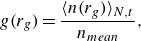(3.4) \begin{align} g(r_g) = \frac {\langle n(r_g)\rangle _{N,t}}{n_{mean}} , \end{align}

where $n_{mean} = N/V$ is the global mean of the number density. The local number density $n(r_g)$ is defined by the number of swimmers within the spherical shell domain of radius $r_g - \Delta r$ to $r_g$ .

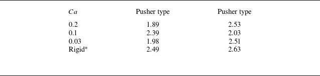
The aggregation ratio $g$ of pushers and pullers is shown in figure 7. Both pushers and pullers tended to aggregate within $r_g \approx 3a$ in all cases, a tendency similar to the rigid squirmers (Ishikawa et al. 2008). However, due to the membrane deformability, soft swimmers aggregated closer than $r_g=2a$ , which is equivalent to the contact distance of rigid swimmers. Higher capillary numbers allowed swimmers to aggregate more closely, but the peak value of $g$ was considerably reduced. Concerning rigid swimmers, the values were high very close to swimmers with $r_g\simeq 2a$ and converged to an average value of 1 at a distance of $r_g \geqslant 3a$ . The number of swimmers forming a cluster is estimated by integrating $\left \langle n(r_g)\right \rangle$ in the region where the swimmer density is grater than the mean. The results are summarised in table 1; in all cases, the clusters were formed by approximately two to three swimmers.

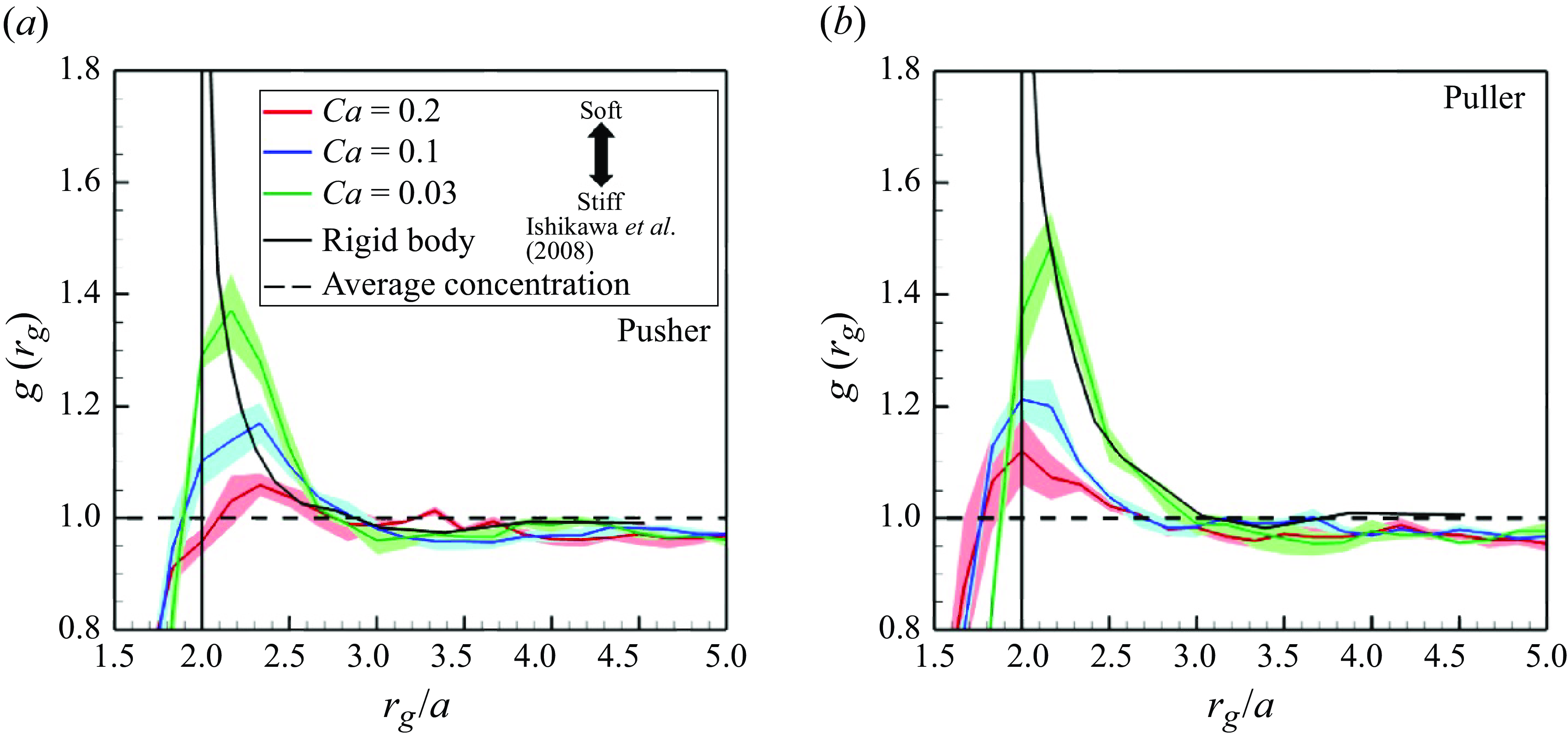
Figure 7. Swimmers’ aggregations in the suspension with $\phi = 0.1$ . The black broken line indicates $g = 1.0$ , where the local number density is equivalent to the global number density. The black sold lines show the result of rigid squirmers (Ishikawa et al. 2008).

Table 1. Average number of swimmers in a unit cluster. The marker ‘*’ shows reference to the previous results of rigid squirmer models provided by Ishikawa et al. (2008).

3.3. Swimming speed

The ensemble average of the swimming speed $\left \langle |\boldsymbol {U}_i|\right \rangle _N(t)$ was computed from $200 \leqslant tU_0/a \leqslant 400$ . The time-averaged value is represented by $\bar {\langle U\rangle }$ . Figure 8 shows $\bar {\langle U\rangle }$ as a function of $\phi$ , with $Ca = 0.03, 0.1$ and $0.2$ . For both pushers and pullers, $\bar {\langle U\rangle }$ monotonically decreased according to $\phi$ . For the same number density and $Ca$ , the average swimming speed of pushers exceeded that of pullers. This is because pushers can more easily pass each other. Among pusher swimmers, a higher $Ca$ value leads to faster swimming under the same number density conditions.

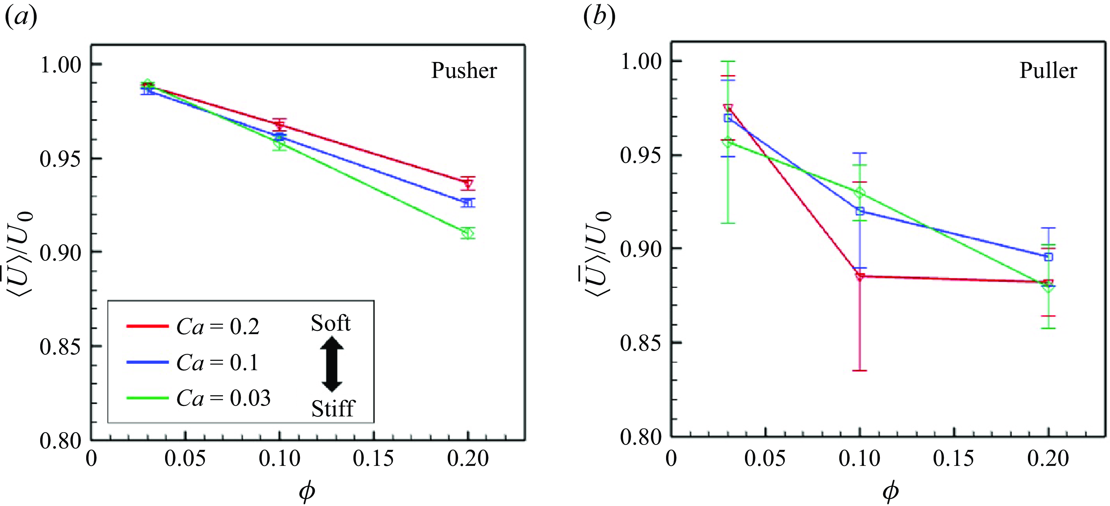
Figure 8. Time-averaged swimming speeds of the swimmers with various $Ca$ . The error bar indicates the standard deviations computed from independent three initial conditions.

Translational dispersion is a measure of microswimmer spreading. The mean square displacement $R^2$ was used to determine the swimmer’s self-dispersion, as given by

(3.5) \begin{align} R^2(\Delta t) = \big\langle | \boldsymbol {r}_i(t + \Delta t) - \boldsymbol {r}_i(t)|^2 \big\rangle _N, \end{align}

where $\boldsymbol {r}$ is the swimmer’s displacement, $\Delta t$ is the time interval and $R^2$ is a function of $\Delta t$ with $\phi = 0.20$ , as shown in figure 9. We observed the different effects of $Ca$ between pushers and pullers. Among pushers, the value was higher for larger $Ca$ in the high $\Delta t$ regime, whereas it was almost invariant for $Ca$ among pullers. In the double logarithmic axes (cf. inset graph in figure9), both pushers and pullers had a slope of 2. Thus, the swimmers’ movement was ballistic, rather than diffusive, in the range of $\Delta t U_0/a \leqslant 100$ . A longer $\Delta t$ analysis may ultimately lead to a transition to diffusion; however, the computational time interval $\Delta tU_0/a \leqslant 100$ is not sufficient to confirm this transition. Since the time scale of the relaxation time for orientational self-correlation is estimated as $O(10^2)$ , a time scale of $O(10^3)$ may be required to observe a diffusion phenomenon, which is difficult to achieve due to the long computational time. The converged values could not be confirmed in this study.

Figure 9. Mean square displacements $R^2$ in the suspension with $\phi = 0.2$ during the time interval $\Delta t$ . The inserted graph is drawn to a double logarithmic scale.

3.4. Rotational diffusivity

Rotational diffusivity $\unicode{x1D63F}_R$ is defined as follows to describe scattering in the swimming direction:

(3.6) \begin{align} \unicode{x1D63F}_R(\Delta t) = \lim _{\Delta t\rightarrow \infty } \frac {\left \langle ( \boldsymbol {\omega }(t + \Delta t) - \boldsymbol {\omega }(t))\otimes ( \boldsymbol {\omega }(t + \Delta t) - \boldsymbol {\omega }(t))\right \rangle _N}{2\Delta t},\\[-24pt]\nonumber \end{align}

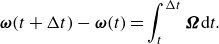(3.7) \begin{align} \boldsymbol {\omega }(t + \Delta t) - \boldsymbol {\omega }(t) = \int ^{\Delta t}_{t} \boldsymbol {\Omega } \mathrm{d}\it t. \end{align}

Here $\boldsymbol {\Omega }$ is the swimmer’s rotational velocity and $\boldsymbol {\omega }$ is the rotational displacement. The average of the diagonal components of $\unicode{x1D63F}_R$ represents the isotropic contribution:

(3.8) \begin{align} \unicode{x1D63F}_R = ({D}_{R,xx} + {D}_{R,yy} + {D}_{R,zz})/3. \end{align}

The time change of $\unicode{x1D63F}_R$ with $\phi = 0.10$ and $0.20$ is shown in figure 10. Here $\unicode{x1D63F}_R$ linearly increases in the small $\Delta t$ regime ( $\Delta t U_0/a \lt 1$ ) and then gradually converges to a specific value at $\Delta t U_0/a \geqslant 10$ . This tendency is similar to that of rigid swimmers (Ishikawa & Pedley 2007). Regarding soft pushers, the converged value was slightly smaller with increasing $Ca$ , which suggests that softer pushers can maintain their swimming direction during the interaction, (i.e. the softer pusher has highly direct swimmability). Among pullers, $\unicode{x1D63F}_R$ was slightly higher with $Ca$ . In addition, we observed long and stable two-body clusters during face-to-face collisions, and $\unicode{x1D63F}_R$ convergence became worse (cf. figure 10 b).

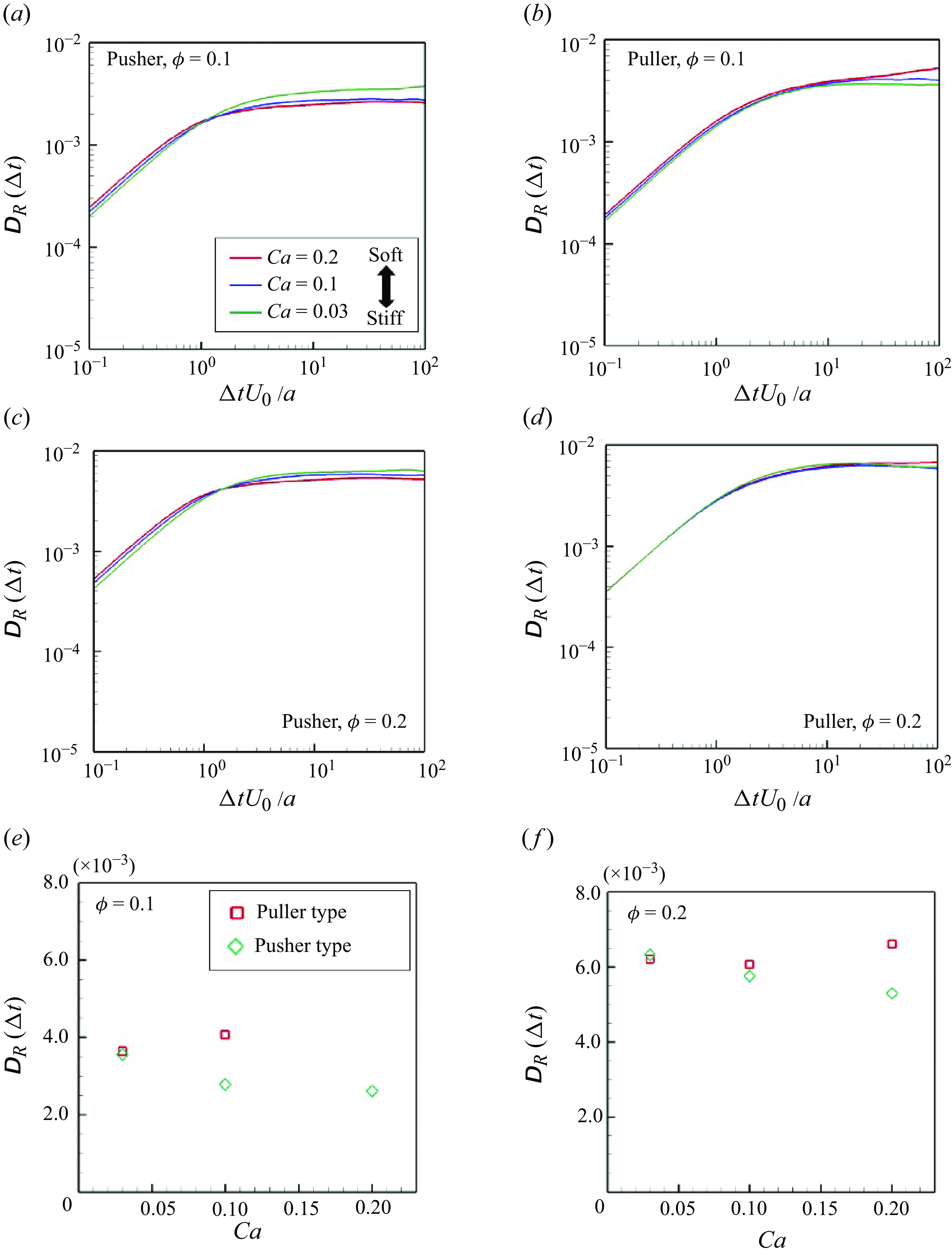
Figure 10. (a–d) Time change of swimmers’ rotational diffusivities during the time interval $\Delta t$ ; (a,b) $\phi = 0.1$ and (c,d) $\phi = 0.2$ . Converged values of $D_R$ in the suspension with (e) $\phi = 0.1$ and (f) $\phi = 0.2$ . (Note that the result of the puller type with $Ca = 0.2$ is excluded because the convergent value has not been obtained during the time scale that has been simulated.)

To further analyse the short-range interactions, the effects of swimming mode on the nearby swimmer distribution were examined. Because most clusters were formed by two or three swimmers (cf. table 1), we focused on the closest two-body interaction. The distributions of the closest swimmers during the short-range interaction were quantified, and the probability density $P$ was derived as a function of $\alpha$ . Here $\alpha$ is the relative angle between the closest swimmers $i$ and $j$ , (i.e. the angle in which the closest swimmer $j$ is from the direction of $\boldsymbol {e}_i$ ):

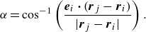(3.9) \begin{align} \alpha = \cos ^{-1} \left ( \frac {\boldsymbol {e}_i \boldsymbol{\cdot} (\boldsymbol {r}_j - \boldsymbol {r}_i)}{|\boldsymbol {r}_j - \boldsymbol {r}_i|} \right ). \end{align}

As shown in figure 11, pushers with low $Ca$ exhibited asymmetric distributions of $P(\alpha )$ , and the peak appeared in the range of $\pi /3 \lt \alpha \lt \pi /2$ . As $Ca$ increases, the peak shifted to $\pi /2$ and the distribution became almost symmetric. With respect to pullers with high $Ca$ , a large peak was observed at $\alpha \lt \pi /12$ , indicating that a soft puller is likely to collide with the head. Among pullers, structures with heads coalesced due to the retracted flow have also been reported for the ellipsoidal squirmers (Kyoya et al. 2015); the results of the present study are consistent with this finding.

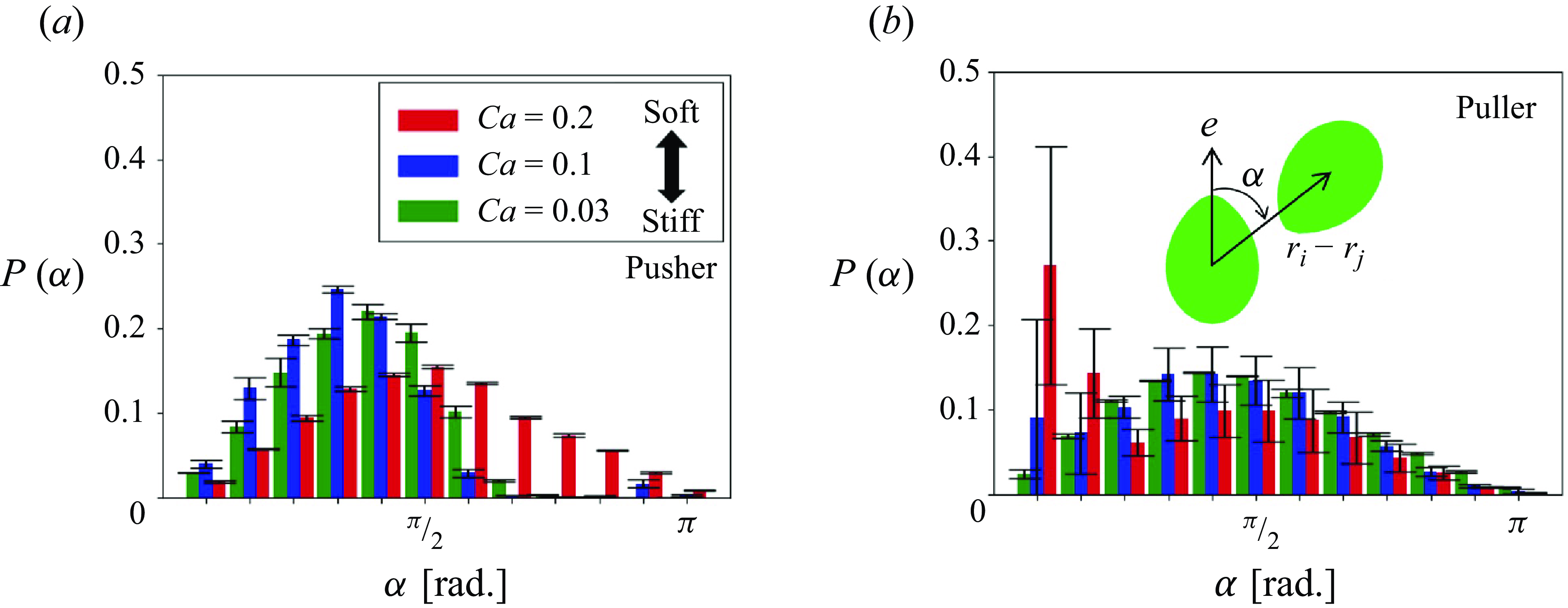
Figure 11. Probability density of the nearest neighbours as a function of relative angle $\alpha$ from the swimming direction ( $\phi = 0.1$ ).

4. Deformation and tension

Membrane tension is important for the analysis of capsule dynamics in a suspension (Walter et al. 2011; Omori et al. 2012). For example, Walter et al. (2011) reported that membrane wrinkling and buckling occurs due to local compression in the low $Ca$ regime, whereas the capsule is extremely elongated at the tip in the high $Ca$ regime. Membrane tension is also associated with mechanosensing mechanisms in swimming microorganisms (Matsui et al. 2020a ). How does the cellular microstructure presented in the previous section relate to the membrane tension of the microswimmer? In this section we investigate the deformation and membrane tension of the microswimmer during many-body hydrodynamic interactions.

4.1. Strain

In order to quantify membrane deformation, we utilised the second invariant of the strain tensor $I_2$ within the short-range interaction ( $r \lt 3a$ ). The second invariant represents the area dilatation of the membrane, which controls the mechanosensitive channel of prokaryotes during severe osmotic challenges (Sukharev et al. 1997; Perozo et al. 2002). The time- and ensemble-averaged strain increment $\Delta I_{2}$ relative to the solitary swimming is presented in figure 12. As indicated in figure 12(a), $\Delta I_{2}$ was nearly proportional to $Ca$ for both pushers and pullers. This phenomenon represents a direct consequence of an increase in $Ca$ , resulting in reduced membrane rigidity. Here $\Delta I_{2}$ was greater for pullers than for pushers, due to the pulling effect in the swimming direction. We also investigated the effect of the volume fraction $\phi$ on deformation (cf. figure 12 b). A linear trend was observed for the volume fraction. A greater volume fraction led to more frequent microswimmer collisions, resulting in larger deformation.

Figure 12. Difference of the second strain invariant from the solitary swimming: (a) effect of $Ca$ ( $\phi = 0.1$ ) and (b) effect of $\phi$ ( $Ca = 0.1$ ).

4.2. Tension

We evaluated the principal tension during the interaction. The principal tension $\tau _1$ of the Skalak law is given by

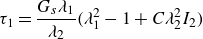(4.1) \begin{align} \tau _{1} = \frac {G_s \lambda _1}{\lambda _2}(\lambda ^2_1 - 1 + C\lambda ^2_2 I_2) \end{align}

and $\tau _{2}$ is obtained by switching $\lambda _1$ and $\lambda _2$ . Because the in-plane isotropic tension $T$ , defined as $T = (\tau _1 + \tau _2)/2$ , could be relevant for activation of the mechanosensing ion channel (Matsui et al. 2020a ), we focused on the in-plane isotropic tension $T$ .

In this study the reference shape of the elastic membrane was assumed to be a sphere. Membrane tension was then generated, even in dilute suspensions without interparticle interactions. The mean value of $T$ in the solitary swimming, $T_{mean}^{sol} = {\int (T { \mathrm{d}}A)}/{A}$ , is shown in figure 13(a), where $A$ is the membrane surface area of the swimmer. Here $T_{mean}^{sol}/\mu U_0$ increased according to $Ca$ . The tension of pushers was always higher than that of pullers because pusher swimmers displayed a dented shape in the back (cf. figure 1), and tended to have a higher $T_{mean}^{sol}$ compared with other swimmer types.

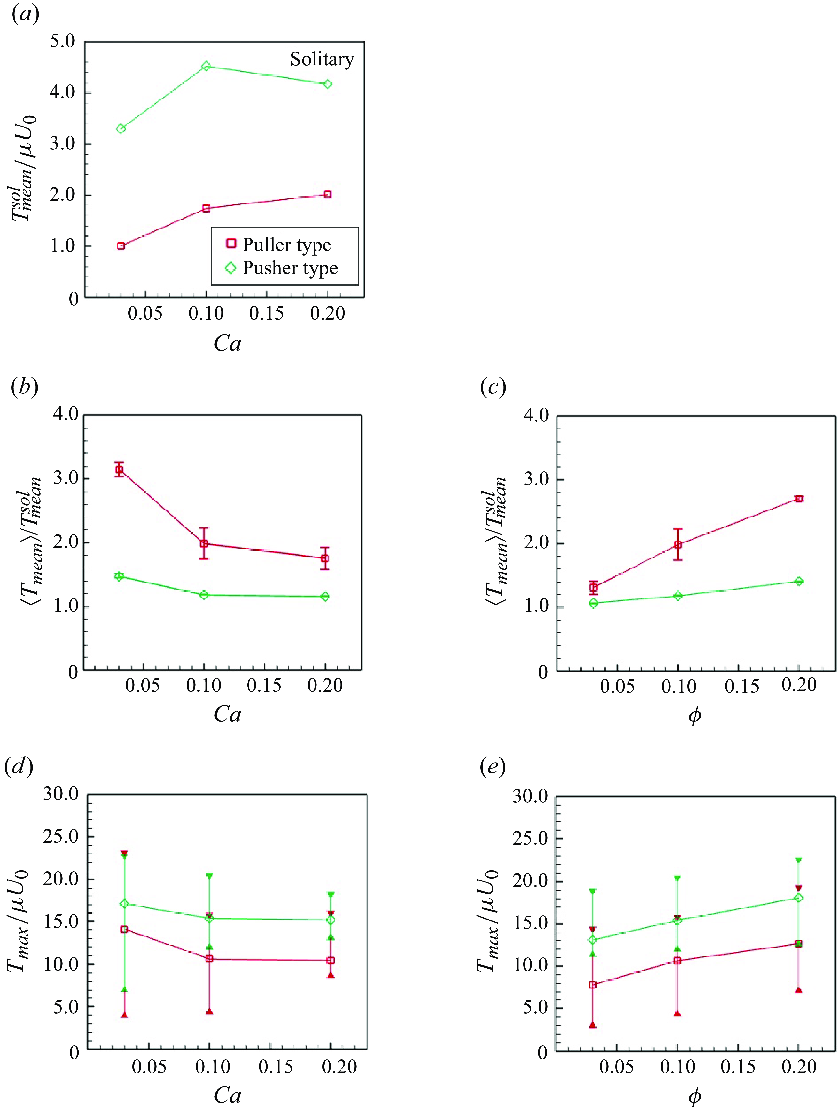
Figure 13. In-plane isotropic tension of swimmers $T (= (\tau _1 + \tau _2)/2)$ . Tensions are derived in each triangular element and then averaged over swimmers and times. (a) Mean tension of the solitary swimming. (b,c) Mean tension normalised by the solitary swimming. (d,e) Time-averaged maximum tension in the suspension. The bar indicates instantaneous maximum and minimum values of the maximum tension in the suspension.

Considering variation in the tension due to the hydrodynamic interactions within the suspension, the averaged incremental tension from the solitary swimming $\langle T_{mean} \rangle _{N,t}/T_{mean}^{sol}$ was lower for pushers (cf. figure 13 b) because they are more likely to pass each other. As shown in figure 13(c), the slip-through effect of pushers was effective even at higher number densities; among the pullers, tension increased according to number density. Regarding pullers, tensions were strongly influenced by $Ca$ . When $Ca = 0.03$ , $\langle T_{mean} \rangle _{N,t}/T_{mean}^{sol}$ was approximately 3.2, and the value monotonically decreased according to $Ca$ .

The instantaneous maximum tension in the suspension was determined; the time averages are shown in figure 13. Both swimmers showed similar trends in $Ca$ and $\phi$ . As $Ca$ increased with fixed $\phi$ , the maximum tension slightly decreased. Softer swimmers were able to avoid hard collisions, potentially explaining why the maximum tension was reduced by $Ca$ , whereas the maximum tension linearly increased according to $\phi$ . The frequency of many-body interferences increased according to number density. Accordingly, the capsular membrane experienced greater tension.

The tension distribution changed with pushing and pulling hydrodynamic interactions. The incremental tension during the short-range interaction was evaluated as a function of the azimuth angle $\theta$ relative to the orientation vector, as defined by $\Delta T(\theta )$ in the following:

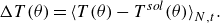(4.2) \begin{align} \Delta T(\theta ) = \big\langle T(\theta ) - T^{sol}(\theta )\big\rangle _{N,t}. \end{align}

Here $T(\theta )$ is the circumferentially averaged isotropic tension at $\theta$ in the suspension and $T^{sol}(\theta )$ is that of solitary swimming. The result is shown in figure 14. In all cases, incremental tension $\Delta T(\theta )$ decreases according to $Ca$ (cf. figures 14 a and 14 b). Pushers showed a relatively flat distribution of $\Delta T(\theta )$ , except at the $\theta = \pi$ pole, whereas pullers tended to have a decreasing $\Delta T(\theta )$ in the $\theta \leqslant \pi /2$ region.

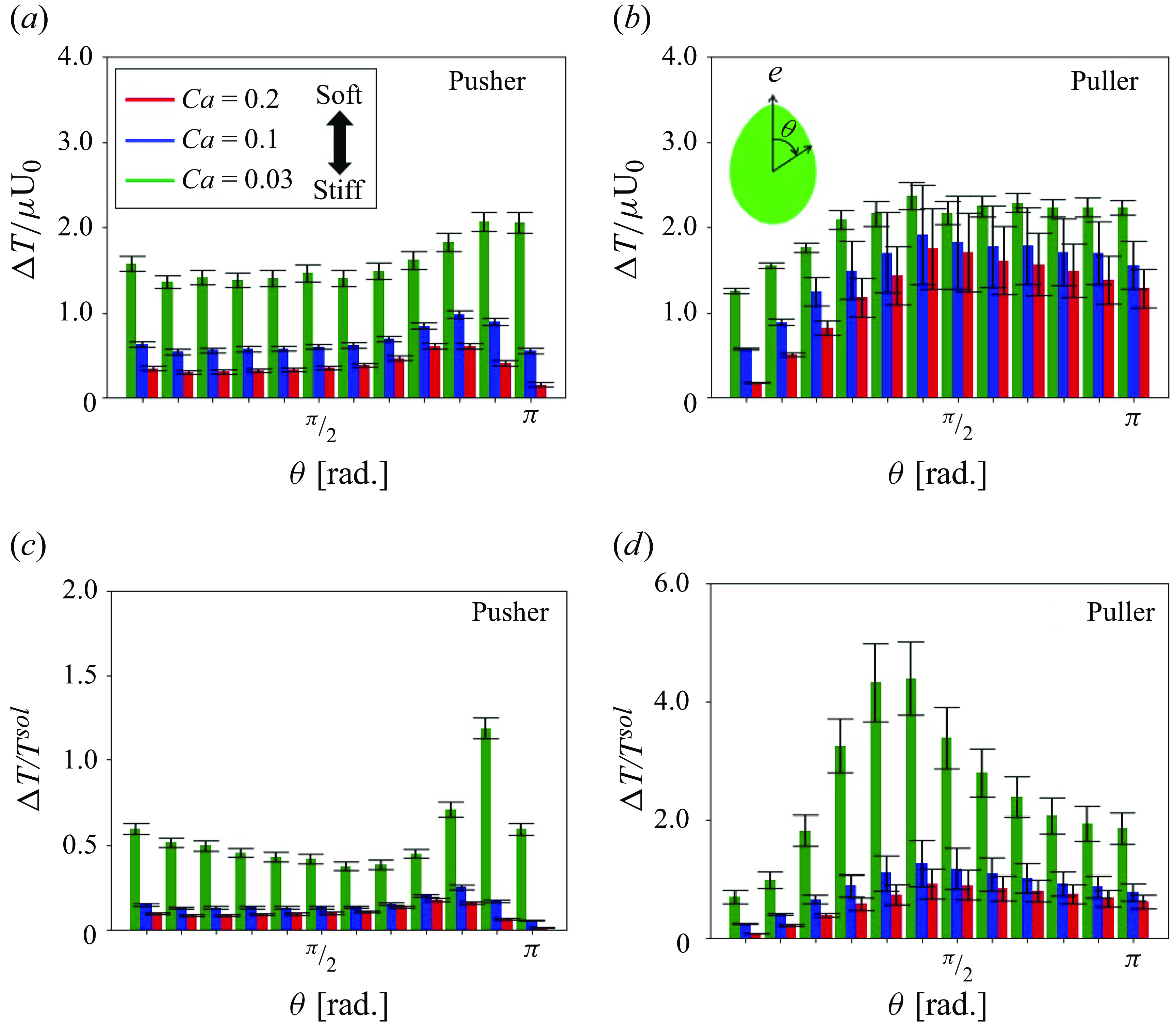
Figure 14. Incremental tension $\Delta T$ as a function of the polar angle on a swimmer surface $\theta$ ( $\phi = 0.1$ ). (a,b) Distributions of local incremental tension $\Delta T$ from the solitary swimming. (c,d) Distributions of the ratio $\Delta T/T_{sol}$ .

Upon further examination of directional distributions that caused the largest tension fluctuations, the incremental tension was normalised according to the value used for solitary swimming. The results are shown in figures 14(c) and 14(d). Among pushers, the ratio of increase was high for $3\pi /4\lt \theta \lt \pi$ ; among pullers, the ratio of increase was high around $\theta = \pi /2$ . These tendencies were more pronounced at low capillary numbers. These results indicate that for pushers (pullers), the greatest change in tension occurs in the posterior (side) during the interaction.

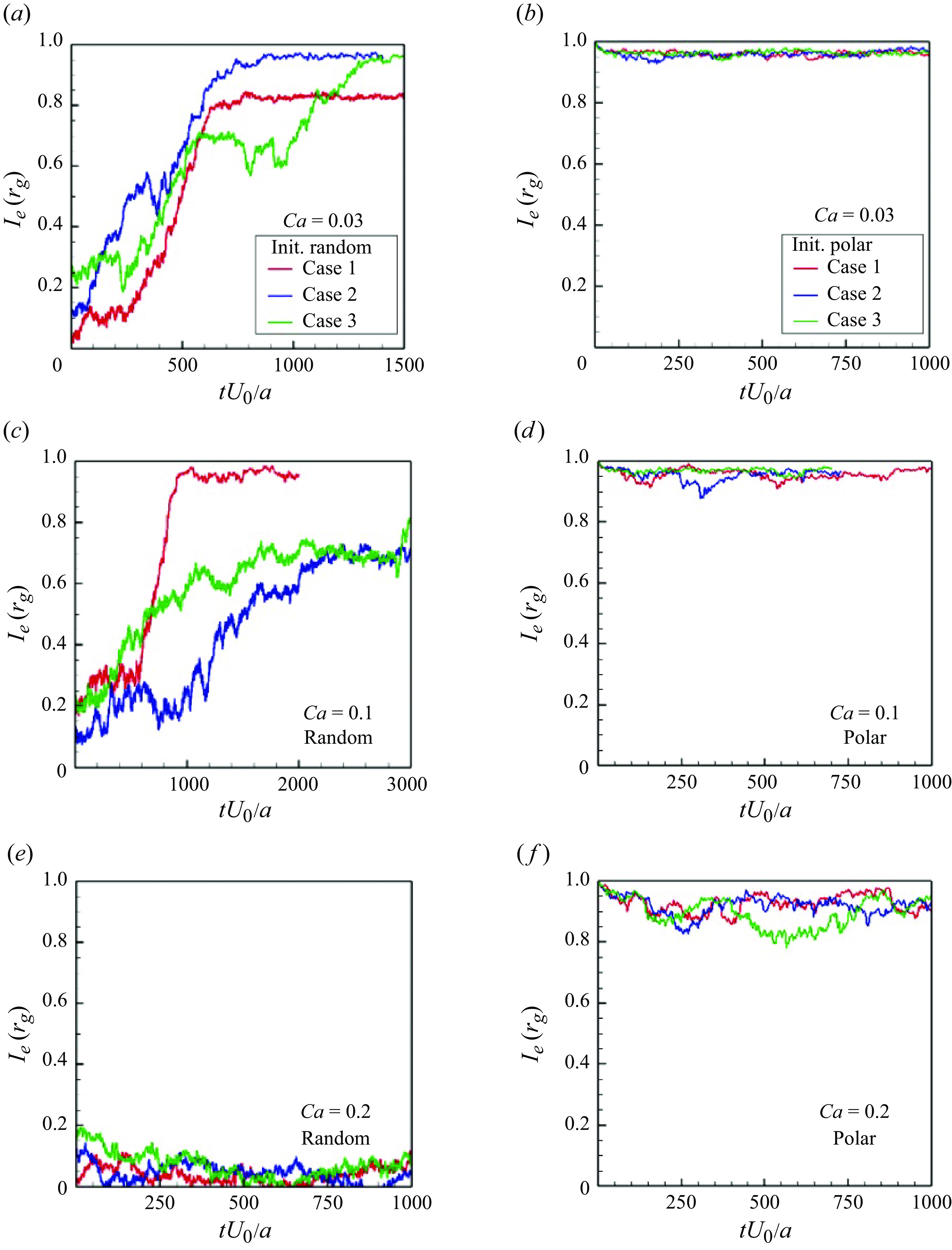
Figure 15. Orientational correlation of the neutral swimmers with $\phi = 0.1$ . Each line indicates three different initial conditions with (a,c,e) showing initially random configurations and (b,d,f) initially polar order configurations.

5. Conclusion

In this study we investigated the elastohydrodynamic interactions of deformable soft microswimmers. Membrane deformation altered the mutual interference between swimmers in the cluster, causing closer interactions compared with rigid squirmers. This deformation enables swimmers to more easily slip through each other, weakening the formation of orientation order through short-range interactions. Especially among soft pushers, rotational diffusion due to hydrodynamic interference was reduced, and swimming in the suspension was relatively straight. This ability, induced by membrane deformability, is useful for the propulsion of cells, such as medical microrobots, and it may play an important role in the transport phenomena for high-concentration cell suspensions. On the other hand, pullers showed more proximity interactions with head collisions due to their retraction flow, and an increase in mean membrane tension. However, high deformability led to loosened contacts and smaller increases in tension. These proximity interaction differences resulted in the positional dependence of the tension in each swimmer mode. For pushers (pullers), the rear (side) interaction produced the greatest change in tension. These findings based on membrane dynamics is expected to contribute to a better understanding of microbial physiological reactions via their mechanotransduction, and to the control of membrane deformation and rupture in medical microrobots for drug delivery. In conclusion, membrane deformability can significantly alter the short-range interactions of the swimmers, such that pushers gain straightness in their trajectories and pullers generate high membrane tension.