


1. Introduction
Fluid flows often contain a range of spatial and temporal features, and since the early work of Reynolds (Reference Reynolds1895), decomposing a flow into modes has been a well-established technique for identifying and distinguishing between distinct features and for reducing the dimensionality of flows (Taira et al. Reference Taira, Brunton, Dawson, Rowley, Colonius, McKeon, Schmidt, Gordeyev, Theofilis and Ukeiley2017). Reynolds (Reference Reynolds1895) proposed one of the first modal decompositions in fluid dynamics, that of a turbulent flow into a time mean and a fluctuation about the mean, a decomposition that was later referred to as the ‘Reynolds decomposition’ and formed the basis of the Reynolds-averaged Navier Stokes approach to turbulence modelling. Approximately 50 years ago, Hussain & Reynolds (Reference Hussain and Reynolds1970a ) introduced the ‘triple decomposition’ of a flow field, which decomposes the unsteady component of a flow into ‘coherent’ and ‘incoherent’ components, and this technique has been used extensively, particularly for flows that contain a dominant low-frequency time scale (Kotapati, Mittal & Cattafesta Reference Kotapati, Mittal and Cattafesta2007; Baj, Bruce & Buxton Reference Baj, Bruce and Buxton2015).
The proper orthogonal decomposition (POD) method was first introduced in fluid dynamics by Lumley (Reference Lumley1967), and it allowed for the decomposition of a flow into an infinite set of orthogonal eigenfunctions or modes. The objective of POD is to identify the dominant modes in the flow and to reduce the dimensionality of the flow, and this method also become extensively employed in the analysis of fluid flows (Rochuon, Trébinjac & Billonnet Reference Rochuon, Trébinjac and Billonnet2006; Zhao et al. Reference Zhao, Zhao, Liu and Du2019). The Fourier transform may be considered to be yet another fundamental modal decomposition that has been applied extensively to fluid flows and has even formed the basis of a class of discretisation methods (Canuto et al. Reference Canuto, Hussaini, Quarteroni and Zang2006).
The rise of data-enabled techniques and machine-learning in the last two decades has led to an explosion of interest and activity in modal decomposition techniques in fluid dynamics (Taira et al. Reference Taira, Brunton, Dawson, Rowley, Colonius, McKeon, Schmidt, Gordeyev, Theofilis and Ukeiley2017), and several new modal decomposition techniques such as dynamic mode decomposition (DMD), spectral POD (SPOD) and resolvents (Schmid Reference Schmid2010; Nekkanti & Schmidt Reference Nekkanti and Schmidt2021; Herrmann et al. Reference Herrmann, Baddoo, Semaan, Brunton and McKeon2021) have appeared on the scene. Almost all modal decomposition techniques are applied to the velocity field, and the modal decomposition can be expressed as
 \begin{equation} \boldsymbol{u}(\boldsymbol{x},t)=\boldsymbol{u}_0(\boldsymbol{x})+\boldsymbol{u}_1(\boldsymbol{x},t)+\cdots +\boldsymbol{u}_i(\boldsymbol{x},t)+\cdots +\boldsymbol{u}_N(\boldsymbol{x},t), \end{equation}
where the terms on the right represent the modes. In most decomposition techniques, the first term on the right-hand side is the time mean flow, and
 $N$
can range from
$N$
can range from
 $N=1$
(as for Reynolds decomposition) to an arbitrarily large number (as for Fourier or POD modal decompositions).
$N=1$
(as for Reynolds decomposition) to an arbitrarily large number (as for Fourier or POD modal decompositions).
As an example, we present the POD of the flow past a circular cylinder, which is a quintessential vortex-dominated flow. Figure 1(a) shows the vortices for flow past a circular cylinder at Reynolds number
 $Re=300$
, and figure 1(c) shows the time variation of the total lift and drag force coefficients, as well as the pressure components of these two coefficients. Figure 2 shows the mean and the first three POD modes obtained from a modal decomposition of the velocity field. These four modes together constitute 94.2 % of the total variance in this flow, and each mode has a distinct topology. For instance, Mode-1 is symmetric about the wake centreline, whereas Mode-2 and Mode-3 are not. Figure 2(e) shows the time-variation of the velocity at one selected point in the wake for each of these three modes, and it is clear that the time variation of these modes is also quite distinct. Thus the POD modes provide important information about the dominant space–time characteristics of the flow.
$Re=300$
, and figure 1(c) shows the time variation of the total lift and drag force coefficients, as well as the pressure components of these two coefficients. Figure 2 shows the mean and the first three POD modes obtained from a modal decomposition of the velocity field. These four modes together constitute 94.2 % of the total variance in this flow, and each mode has a distinct topology. For instance, Mode-1 is symmetric about the wake centreline, whereas Mode-2 and Mode-3 are not. Figure 2(e) shows the time-variation of the velocity at one selected point in the wake for each of these three modes, and it is clear that the time variation of these modes is also quite distinct. Thus the POD modes provide important information about the dominant space–time characteristics of the flow.
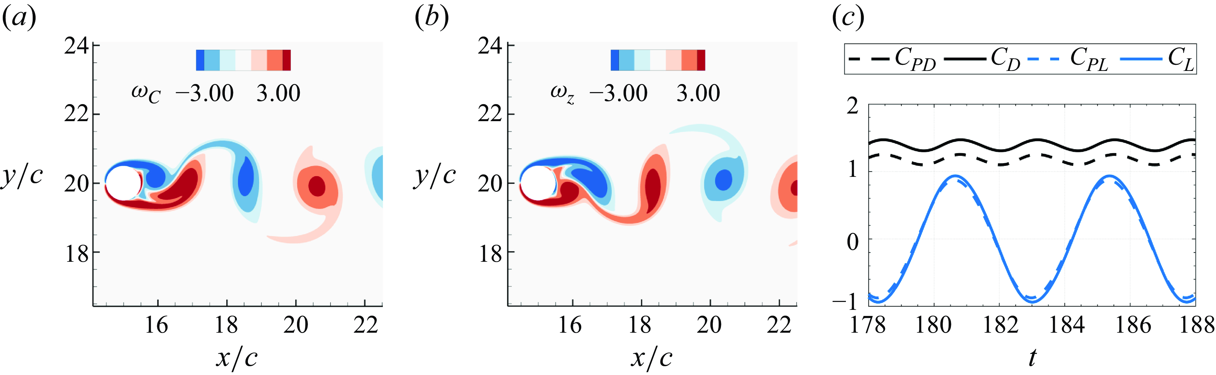
Figure 1. (a,b) Spanwise vorticity corresponding to flow past a circular cylinder at Reynolds number 300, showing the shedding of the vortices in the wake at two instances. (c) Time variation of coefficients of drag and lift (pressure-induced and total) for the circular cylinder.
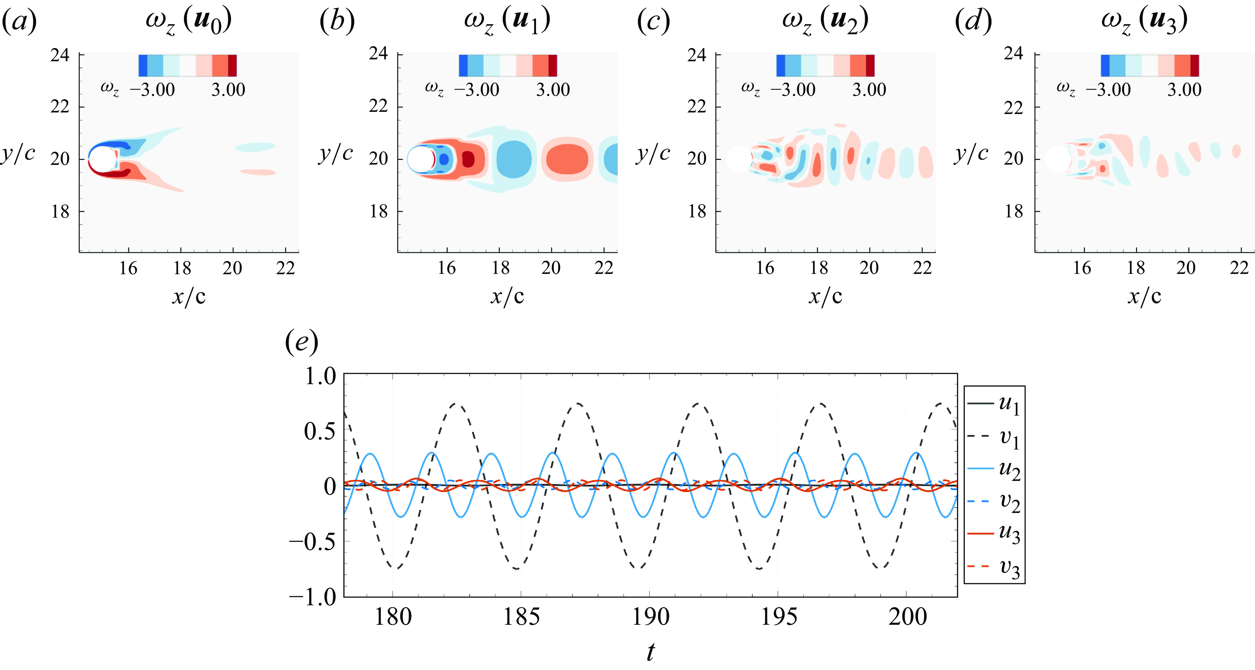
Figure 2. The POD applied to the cylinder flow. Spanwise vorticity for (a) the mean mode (Mode-0), (b) Mode-1, (c) Mode-2, and (d) Mode-3. (e) Time variation of the streamwise and lateral velocity at downstream distance
 $d$
from the centre of the cylinder on the wake centreline.
$d$
from the centre of the cylinder on the wake centreline.
The modes that are generated from POD (as well as from other decomposition methods) are, however, purely kinematic in their description, i.e. they are designed for an examination of the topological characteristics of the flow field, but they do not directly provide any information on the dynamics of the flow. In particular, we do not have the ability to determine the contributions that these modes make to the fluid dynamic forces on the submerged body. Such a capability would be extremely useful in several applications, including the following.
-
(i) Determining the contribution of these modes to fluid dynamic loads (lift, drag, moments, etc.). Aerodynamic loads are key in a majority of scientific investigations and engineering applications that involve fluid flow, and being able to quantify the aerodynamic loads associated with these modes could provide important insights into the flow physics associated with the generation of these forces. For instance, the symmetry properties of Mode-1 indicate that it contributes to drag but not to the lift force on the cylinder, Mode-2 and Mode-3 will contribute to the lift and the drag on the cylinder. However, we have no means of quantifying these contributions.
-
(ii) Understanding the contribution of decomposed modes to flow-induced vibration and flutter (FIVF). The FIVF is determined by the phasing between the fluid dynamic loads and the movement of the structure, and since each mode typically has a distinct temporal profile, the ability to estimate the time variation of the loads associated with each mode would provide a unique ability to analyse FIVF.
-
(iii) Analysis of the sources of flow noise. Unsteady pressure loading of immersed surfaces serves as a source of flow noise (Howe Reference Howe2002) in applications ranging from aeronautics (Brentner & Farassat Reference Brentner and Farassat1994) and marine engineering (Ianniello, Muscari & Di Mascio Reference Ianniello, Muscari and Di Mascio2013) to bio-medicine (Bailoor et al. Reference Bailoor, Seo, Schena and Mittal2021) and zoology (Nedunchezian, kwon Kang & Aono Reference Nedunchezian, Kang and Aono2019). Thus correlating the sources of flow noise to distinct flow modes could be very insightful.
-
(iv) Developing physics-driven strategies for flow control. Effective flow control for applications such as drag reduction, lift/thrust enhancement, reduction/enhancement of FIVF, or reduction in flow noise, could be empowered by understanding the contribution of modes to the relevant fluid dynamic loads induced by these modes. Control strategies could then be designed to systematically target those modes that make dominant contributions to these loads.
There have been some previous attempts to determine the fluid dynamic loads associated with the modal decomposition of flows. For instance, Mittal & Balachandar (Reference Mittal and Balachandar1995) decomposed the velocity field past a circular cylinder obtained from a three-dimensional (3-D) spanwise homogeneous simulation into a spanwise-averaged component and the remnant 3-D mode as
 $\boldsymbol{u}(x,y,z,t) = \bar {\boldsymbol{u}}^{2\text{-}D}(x,y,t) + \boldsymbol{u}^{3\text{-}D}(x,y,z,t)$
, then solved the pressure Poisson equation for each mode to partition the contributions of these two modes to the pressure drag over the cylinder. This allowed them to determine the contributions that 3-D flow features make to the total drag and lift forces on the cylinder, and pinpoint the cause for the over-prediction of drag in two-dimensional (2-D) simulations of these flows.
$\boldsymbol{u}(x,y,z,t) = \bar {\boldsymbol{u}}^{2\text{-}D}(x,y,t) + \boldsymbol{u}^{3\text{-}D}(x,y,z,t)$
, then solved the pressure Poisson equation for each mode to partition the contributions of these two modes to the pressure drag over the cylinder. This allowed them to determine the contributions that 3-D flow features make to the total drag and lift forces on the cylinder, and pinpoint the cause for the over-prediction of drag in two-dimensional (2-D) simulations of these flows.
Aghaei-Jouybari et al. (Reference Aghaei-Jouybari, Seo, Yuan, Mittal and Meneveau2022) deployed the force partitioning method (FPM) (Zhang, Hedrick & Mittal Reference Zhang, Hedrick and Mittal2015; Menon & Mittal Reference Menon and Mittal2021
Reference Menon and Mittal
a
,Reference Menon and Mittal
c
) to decompose and analyse the pressure-induced drag for turbulent flow over rough walls. More details of the FPM, which is based on the earlier work of Wu (Reference Wu1981), Quartapelle & Napolitano (Reference Quartapelle and Napolitano1983), Chang (Reference Chang1992), Howe (Reference Howe1995) and Zhang et al. (Reference Zhang, Hedrick and Mittal2015), will be provided in § 2.2 since it is central to the current paper, but it suffices for now to point out that the FPM enables the partitioning of the pressure drag over the roughness elements into a component due to flow vorticity (the so-called ‘vortex-induced’ component) and a component due to the viscous diffusion of momentum. The analysis was performed on data from direct numerical simulations of turbulent channel flows, at frictional Reynolds number
 $Re_\tau=500$
, with cubic and sand-grain roughened bottom walls. The results from these simulations showed that the vortex-induced pressure drag is the largest contributor (more than 50 %) to the total drag (which is the sum of pressure and shear drag) on the rough walls. A Reynolds decomposition of the flow into mean and fluctuation components was also performed, and the contributions of these two modes on the mean drag were estimated using the FPM and found to be nearly equal.
$Re_\tau=500$
, with cubic and sand-grain roughened bottom walls. The results from these simulations showed that the vortex-induced pressure drag is the largest contributor (more than 50 %) to the total drag (which is the sum of pressure and shear drag) on the rough walls. A Reynolds decomposition of the flow into mean and fluctuation components was also performed, and the contributions of these two modes on the mean drag were estimated using the FPM and found to be nearly equal.
Zhu et al. (Reference Zhu, Lee, Kumar, Menon, Mittal and Breuer2023) applied the force and moment partitioning method (FMPM) of Menon & Mittal (Reference Menon and Mittal2021a ) to experimental data for a NACA 0012 wing undergoing sinusoidal pitching in quiescent water. The velocity field was obtained from 2-D particle image velocimetry measurements at the central spanwise plane of the foil. The data were phase-averaged, and the FMPM was applied to this phase-averaged component. The FMPM analysis enabled the separation of the pitching-moment contributions from the leading-edge and trailing-edge vortices, and their ratio was found to match empirical correlations.
Chiu et al. (Reference Chiu, Tseng, Chang and Chou2023) explored the influence of coherent structures on aerodynamic forces by using SPOD and ‘force representation theory’. This force representation theory is based on Chang (Reference Chang1992), which is also based on the ideas of Quartapelle & Napolitano (Reference Quartapelle and Napolitano1983). Chiu et al. (Reference Chiu, Tseng, Chang and Chou2023) found, for instance, that the large vortex structure in the zeroth frequency mode of the first SPOD mode significantly impacted the lift and drag by inducing strong suction-side flow. This work will be discussed further in the paper since it has connections to the current work.
Finally, Seo et al. (Reference Seo, Zhang, Mittal and Cattafesta2023) introduced a data-driven method for predicting vortex-induced sound from time-resolved velocimetry data and applied it to flow through the slat of a multi-element high-lift aerofoil. Time-resolved particle image velocimetry provided velocity fields in the slat-cove region of the aerofoil, and these were reconstructed using rank-one modes from SPOD. The pressure force and resulting dipole sound were calculated using force (Zhang et al. Reference Zhang, Hedrick and Mittal2015; Menon & Mittal Reference Menon and Mittal2021 Reference Menon and Mittal a ,Reference Menon and Mittal c ) and acoustic partitioning (Seo, Menon & Mittal Reference Seo, Menon and Mittal2022) methods (FAPMs), involving volume integrals of the velocity gradient tensor’s second invariant and geometry-dependent influence fields. Comparisons with measured sound data indicated that while shear layer modes contribute to tonal noise, their interaction with other wing components also generates significant flow noise.
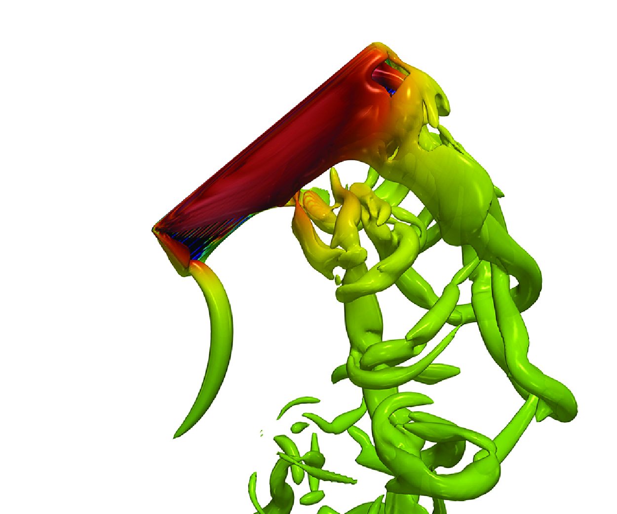
Our current work has been motivated by the problem of aeroacoustic noise from small drones that operate at low tip Mach numbers. As drones are transforming several industries such as transportation, healthcare, vaccine delivery (Lamptey & Serwaa Reference Lamptey and Serwaa2020), rescue operations (Laksham Reference Laksham2019) and food delivery, the noise that they produce during flight is one of the major factors limiting their wide-scale use in several of these applications (Candeloro, Ragni & Pagliaroli Reference Candeloro, Ragni and Pagliaroli2022). This makes reducing noise from drone rotors an important goal. However, the aeroacoustic noise from drones operating at low Mach numbers consists primarily of thickness noise and loading noise. The quadruple noise source that can contribute to broadband noise is negligible at these low Mach numbers. Thickness noise is relatively easy to estimate, but the latter is connected with the pressure loading of the blade, and these depend on the intrinsic unsteadiness in the blade loading vector due to rotation, flow separation and blade vortex interaction (Glegg & Devenport Reference Glegg and Devenport2017). Studies on drone rotor blades indicate complex vortical topologies and dynamics (Misiorowski, Gandhi & Oberai Reference Misiorowski, Gandhi and Oberai2019; Mittal, Seo & Raghav Reference Mittal, Seo and Raghav2021), and all these flow structures present in the flow potentially affect the surface pressure on the blade. This makes the problem of understanding the causality of noise sources quite difficult. The ability to identify key flow features (or modes) that contribute most to the blade loading noise could enable us to pinpoint aspects in the shape and operation of these blades that could reduce the noise.
In the present study, we demonstrate the application of the modal FPM (mFPM) to estimate the pressure loading generated by the modes in the flow that result from various modal decompositions. We apply this methodology to three widely used modal decomposition techniques: the Reynolds decomposition, where any flow quantity can be split into a mean part and a fluctuating component; the triple decomposition (Hussain & Reynolds Reference Hussain and Reynolds1970b ), which further splits the fluctuating part into coherent and non-coherent components; and finally the POD (Berkooz, Holmes & Lumley Reference Berkooz, Holmes and Lumley1993; Chatterjee Reference Chatterjee2000), which segments the flow into modes that are orthogonal and arranged by their decreasing energy content. This mFPM is applied first to a canonical case of flow past a 2-D circular cylinder and the case of 2-D flow past an NACA 0015 aerofoil to understand the fundamental mechanism for unsteady force and sound generation. We use these cases to propose a flow observable that provides a clearer identification of modes that make dominant contributions to the unsteady pressure loading on the immersed bodies. The method is then applied to the flow over a rotating blade to investigate the dominant flow structures associated with generation of loading noise.
2. Methodology
2.1. Flow solver
The flow simulations are done by using a sharp-interface immersed boundary method based incompressible Navier–Stokes solver called ViCar3D (Mittal et al. Reference Mittal, Dong, Bozkurttas, Najjar, Vargas and von Loebbecke2008; Seo & Mittal Reference Seo and Mittal2011). In this solver, the body is represented using unstructured triangular elements that are immersed in a non-uniform Cartesian grid with a discrete-forcing scheme coupled with ghost cells inside the body that can apply boundary conditions precisely on the body surface. The fractional step method of Van Kan (Reference Van Kan1986) is used to split the momentum equation into an advection–diffusion equation and a pressure Poisson equation. The advection–diffusion equation is discretised using a second-order Adams–Bashforth scheme for the convective term, and an implicit Crank–Nicolson method for viscous terms, while the pressure Poisson equation is solved using the gradient descent method. This solver has been validated for complex 2-D and 3-D cases that can be found in Mittal et al. (Reference Mittal, Dong, Bozkurttas, Najjar, Vargas and von Loebbecke2008, Reference Mittal, Seo, Turner, Kumar, Prakhar and Zhou2025) and Mittal & Seo (Reference Mittal and Seo2023).
2.2. FPM
In aerodynamics, the forces due to vortices play an important role, but it is difficult to compute them because the pressure field is an elliptic variable that is calculated by solving a Laplace equation, hence total pressure force is continuously being influenced by all the flow features. The FPM (Menon & Mittal Reference Menon and Mittal2021a ,Reference Menon and Mittal b ,Reference Menon and Mittal c ) helps to overcome this problem and allows us to decompose the pressure forces into four components. These components are the forces generated due to vortices (vortex-induced force), movement/acceleration of the body (we have called this the ‘kinematic force’), acceleration of body or fluid (added mass force), and force due to viscous effects (viscous force). This is done by taking the velocity field calculated before and projecting it onto the Laplace equation
 \begin{equation} \boldsymbol{\nabla} ^2\phi ^{(i)}=0 \end{equation}
with boundary conditions
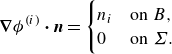 \begin{equation} \boldsymbol{\nabla} \phi ^{(i)} \boldsymbol{\cdot} \boldsymbol{n}= \begin{cases} n_i & \text{on $B$},\\ 0 & \text{on $\Sigma $}. \end{cases} \end{equation}
Here,
 $\phi$
is the ‘influence field’,
$\phi$
is the ‘influence field’,
 $i=1,2,3$
corresponds to the
$i=1,2,3$
corresponds to the
 $x,y,z$
directions,
$x,y,z$
directions,
 $n_i$
represents a normal direction vector,
$n_i$
represents a normal direction vector,
 $B$
is the boundary of the immersed surface, and
$B$
is the boundary of the immersed surface, and
 $\Sigma$
is the domain boundary.
$\Sigma$
is the domain boundary.
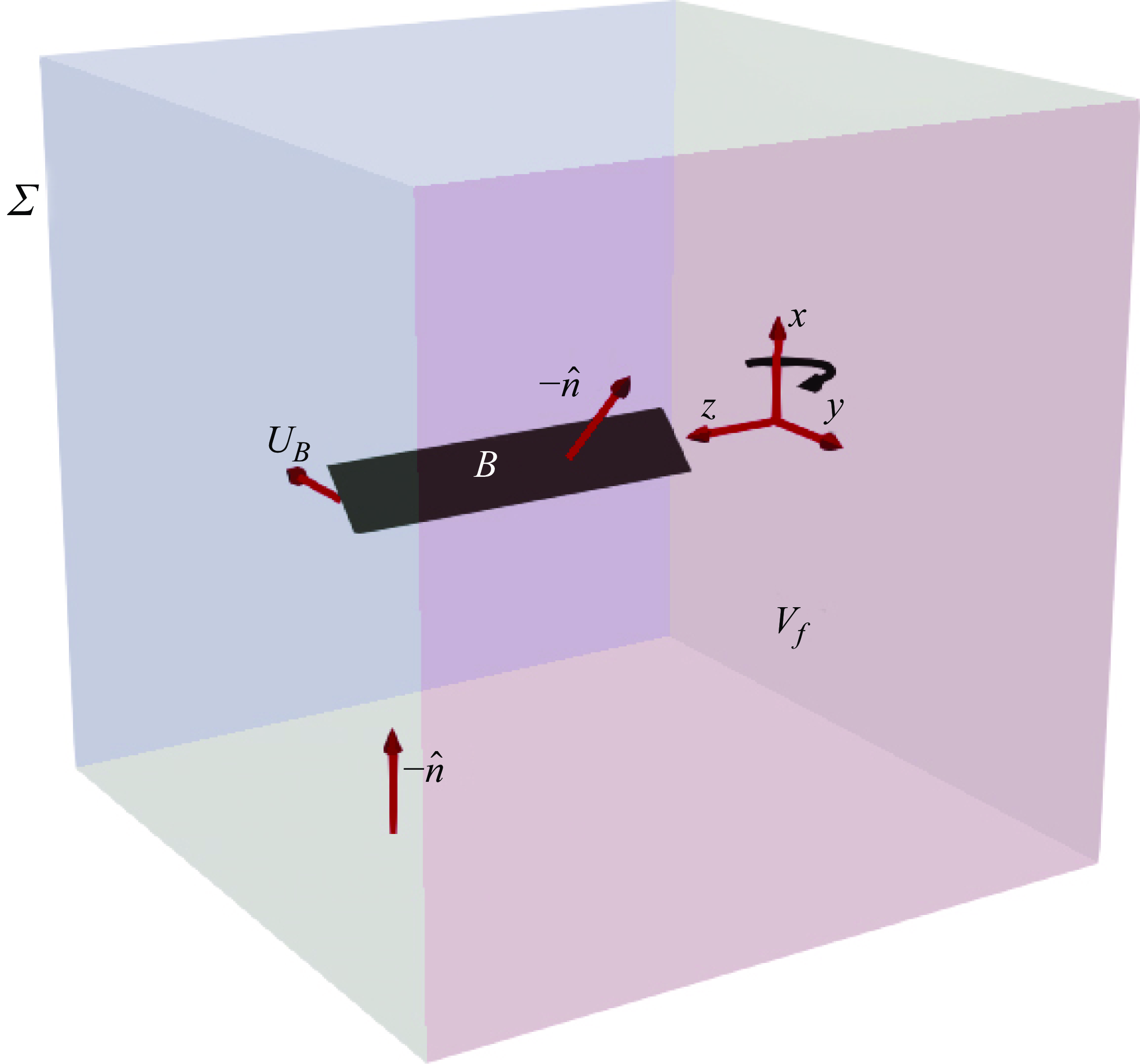
Figure 3. An FPM schematic (not to scale) for the revolving wing, with the origin shown at the centre of revolution.
Then the Navier–Stokes equation
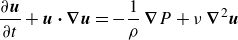 \begin{equation} \frac {\partial \boldsymbol{u}}{\partial t} + \boldsymbol{u}\boldsymbol{\cdot} \boldsymbol{\nabla} \boldsymbol{u} = -\frac {1}{\rho }\,\boldsymbol{\nabla} P +\nu\, \boldsymbol{\nabla} ^2 \boldsymbol{u} \end{equation}
is projected onto the gradient of field of influence potential
 $\phi$
. Rearranging and integrating over the fluid domain gives
$\phi$
. Rearranging and integrating over the fluid domain gives
 \begin{equation} -\int _{V_f}{\boldsymbol{\nabla}} P \boldsymbol{\cdot} {\boldsymbol{\nabla}} \phi ^{(i)}\, {\rm d}V= \int _{V_f} \rho \left [\frac {\partial \boldsymbol{u}}{\partial t} + \boldsymbol{u} \boldsymbol{\cdot} \boldsymbol{\nabla} \boldsymbol{u} - \nu\, \boldsymbol{\nabla} ^2 \boldsymbol{u} \right ]\boldsymbol{\cdot} \boldsymbol{\nabla} \phi ^{(i)}\, {\rm d}V . \end{equation}
This equation can be simplified as (refer to Appendix A)
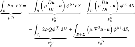 \begin{align} \underbrace {\int _B P n_i\, {\rm d}S}_{F^{(i)}} ={}& \underbrace {-\int _B\left ( \rho \frac {D\boldsymbol{u}}{Dt} \boldsymbol{\cdot} \boldsymbol{n} \right ) \phi ^{(i)}\, {\rm d}S}_{F^{(i)}_B} - \underbrace {\int _\Sigma \left ( \rho \frac {D\boldsymbol{u}}{Dt} \boldsymbol{\cdot} \boldsymbol{n} \right ) \phi ^{(i)}\, {\rm d}S}_{F^{(i)}_O}\nonumber \\ &{}- \underbrace {\int _{V_f} 2 \rho Q \phi ^{(i)}\, {\rm d}V}_{F^{(i)}_Q} +\underbrace {\int _{B+\Sigma } \left ( \mu\, \boldsymbol{\nabla} ^2 \boldsymbol{ u \cdot n} \right ) \phi ^{(i)}\, {\rm d}S}_{F^{(i)}_\mu }, \end{align}
where the term on the left-hand side corresponds to the pressure loading on the body, and terms on the right-hand side correspond respectively to force due to:
 $F_{B}$
, the acceleration reaction due to the motion of the body;
$F_{B}$
, the acceleration reaction due to the motion of the body;
 $F_{O}$
, the added mass force due to material acceleration of the flow on the outer boundary;
$F_{O}$
, the added mass force due to material acceleration of the flow on the outer boundary;
 $F_Q$
, the vortex-induced force; and
$F_Q$
, the vortex-induced force; and
 $F_\mu$
, the force due to viscous diffusion of momentum. Here,
$F_\mu$
, the force due to viscous diffusion of momentum. Here,
 $Q$
is from the so-called
$Q$
is from the so-called
 $Q$
-criterion (Hunt, Wary & Moin Reference Hunt, Wary and Moin1988), defined as
$Q$
-criterion (Hunt, Wary & Moin Reference Hunt, Wary and Moin1988), defined as
 \begin{equation} Q=\tfrac {1}{2} (\| \boldsymbol{\Omega }\|^2- \| \boldsymbol{S}\|^2) \equiv -\tfrac {1}{2}{\boldsymbol{\nabla}} \boldsymbol{\cdot} (\boldsymbol{u}\boldsymbol{\cdot} {\boldsymbol{\nabla}} \boldsymbol{u}) , \end{equation}
where
 $\boldsymbol{S}$
and
$\boldsymbol{S}$
and
 $\boldsymbol{\Omega }$
are symmetric and anti-symmetric components of the velocity gradient tensor, respectively. The derivation and application of the FPM to several flows can be found in Menon & Mittal (Reference Menon and Mittal2021
Reference Menon and Mittal
a
,Reference Menon and Mittal
b
,Reference Menon and Mittal
c
). It should be noted that the above partitioning is exact, and in principle, all of the terms in the partitioning can be estimated from the simulation data (see Zhang et al. Reference Zhang, Hedrick and Mittal2015; Menon & Mittal Reference Menon and Mittal2021c
). For the moderate to high Reynolds number flows that are the subject of the current paper, the pressure force due to viscous momentum diffusion effects are generally small. For instance, for the aerofoil case in § 3.2, the viscous diffusion term contributes less than 4 % to the total pressure lift. Furthermore,
$\boldsymbol{\Omega }$
are symmetric and anti-symmetric components of the velocity gradient tensor, respectively. The derivation and application of the FPM to several flows can be found in Menon & Mittal (Reference Menon and Mittal2021
Reference Menon and Mittal
a
,Reference Menon and Mittal
b
,Reference Menon and Mittal
c
). It should be noted that the above partitioning is exact, and in principle, all of the terms in the partitioning can be estimated from the simulation data (see Zhang et al. Reference Zhang, Hedrick and Mittal2015; Menon & Mittal Reference Menon and Mittal2021c
). For the moderate to high Reynolds number flows that are the subject of the current paper, the pressure force due to viscous momentum diffusion effects are generally small. For instance, for the aerofoil case in § 3.2, the viscous diffusion term contributes less than 4 % to the total pressure lift. Furthermore,
 $F_{B}$
is identically zero for stationary bodies, and for the rotor rotating at constant angular velocity, the magnitude of this term is quite negligible. Finally, since the outer domain is placed far from the body, and the incoming flow is steady in all the cases studied here,
$F_{B}$
is identically zero for stationary bodies, and for the rotor rotating at constant angular velocity, the magnitude of this term is quite negligible. Finally, since the outer domain is placed far from the body, and the incoming flow is steady in all the cases studied here,
 $F_{O}$
is also negligible. Thus, assuming the application of this method for such flows, we proceed with the following approximation for the current study:
$F_{O}$
is also negligible. Thus, assuming the application of this method for such flows, we proceed with the following approximation for the current study:
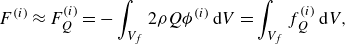 \begin{equation} \begin{aligned} F^{(i)} \approx F^{(i)}_Q = - \int _{V_f} 2 \rho Q \phi ^{(i)}\, {\rm d}V = \int _{V_f} {f^{(i)}_Q}\, {\rm d}V, \end{aligned} \end{equation}
where
 ${f^{(i)}_Q}= - 2 \rho Q \phi ^{(i)}$
is the vortex-force density for the pressure force in the
${f^{(i)}_Q}= - 2 \rho Q \phi ^{(i)}$
is the vortex-force density for the pressure force in the
 $i$
th direction. Note that the force due to individual vortices can be calculated by taking appropriate regions for the above integral (see Menon & Mittal Reference Menon and Mittal2021c
), such as over individual vortices.
$i$
th direction. Note that the force due to individual vortices can be calculated by taking appropriate regions for the above integral (see Menon & Mittal Reference Menon and Mittal2021c
), such as over individual vortices.
2.3. mFPM
For Reynolds decomposition and
 $N=1$
,
$N=1$
,
 $\boldsymbol{u}_0$
is the mean mode calculated as
$\boldsymbol{u}_0$
is the mean mode calculated as
 \begin{equation} \boldsymbol{u}_0(\boldsymbol{x})=\frac {1}{T} \int _{t_0}^{t_0+T} \boldsymbol{u}(\boldsymbol{x},t)\, {\rm d}t , \end{equation}
and
 $\boldsymbol{u}_1(\boldsymbol{x},t)$
is the fluctuation about the mean calculated using
$\boldsymbol{u}_1(\boldsymbol{x},t)$
is the fluctuation about the mean calculated using
 \begin{equation} \boldsymbol{u}_1(\boldsymbol{x},t)= \boldsymbol{u}(\boldsymbol{x},t)- \boldsymbol{u}_0(\boldsymbol{x}) . \end{equation}
For triple decomposition,
 $N=2$
with the mean velocity calculated using (2.8). Here,
$N=2$
with the mean velocity calculated using (2.8). Here,
 $\boldsymbol{u}_1(\boldsymbol{x},t)$
and
$\boldsymbol{u}_1(\boldsymbol{x},t)$
and
 $\boldsymbol{u}_2(\boldsymbol{x},t)$
are the ‘coherent’ and ‘incoherent’ models of the flow. For
$\boldsymbol{u}_2(\boldsymbol{x},t)$
are the ‘coherent’ and ‘incoherent’ models of the flow. For
 $M$
periods of data with an intrinsic time period
$M$
periods of data with an intrinsic time period
 $\tau$
, these are calculated using (Mittal, Simmons & Najjar Reference Mittal, Simmons and Najjar2003)
$\tau$
, these are calculated using (Mittal, Simmons & Najjar Reference Mittal, Simmons and Najjar2003)
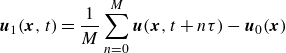 \begin{equation} \boldsymbol{u}_1(\boldsymbol{x},t)= \frac {1}{M} \sum _{n=0}^{M} \boldsymbol{u}(\boldsymbol{x},t+n\tau )- \boldsymbol{u}_0(\boldsymbol{x}) \end{equation}
and
 \begin{equation} \boldsymbol{u}_2(\boldsymbol{x},t)= \boldsymbol{u}(\boldsymbol{x},t)- \boldsymbol{u}_0(\boldsymbol{x}) - \boldsymbol{u}_1(\boldsymbol{x},t) . \end{equation}
For POD,
 $i=1,N$
correspond to the
$i=1,N$
correspond to the
 $N$
POD modes of the flow. We first subtract the mean flow, and as before, this is designated as
$N$
POD modes of the flow. We first subtract the mean flow, and as before, this is designated as
 $\boldsymbol{u}_0(\boldsymbol{x})$
. In the snapshot POD (Sirovich Reference Sirovich1987) approach employed here, the fluctuating velocity (
$\boldsymbol{u}_0(\boldsymbol{x})$
. In the snapshot POD (Sirovich Reference Sirovich1987) approach employed here, the fluctuating velocity (
 $\boldsymbol{u}(\boldsymbol{x},t)- \boldsymbol{u}_0(\boldsymbol{x})$
) at
$\boldsymbol{u}(\boldsymbol{x},t)- \boldsymbol{u}_0(\boldsymbol{x})$
) at
 $m$
selected grid points at a given time step is arranged in a column vector, and these vectors for
$m$
selected grid points at a given time step is arranged in a column vector, and these vectors for
 $N$
sequential time steps are stacked to form
$N$
sequential time steps are stacked to form
 $W$
, an
$W$
, an
 $m \times N$
matrix (Weiss Reference Weiss2019; Wang, McBee & Iliescu Reference Wang, McBee and Iliescu2016). Here,
$m \times N$
matrix (Weiss Reference Weiss2019; Wang, McBee & Iliescu Reference Wang, McBee and Iliescu2016). Here,
 $m$
may be the entire grid or a subset of the grid points. The POD is obtained via the singular value decomposition (SVD) algorithm where
$m$
may be the entire grid or a subset of the grid points. The POD is obtained via the singular value decomposition (SVD) algorithm where
 $W$
is decomposed as
$W$
is decomposed as
 \begin{equation} W=U \Sigma V^{\rm T}, \end{equation}
where
 $U$
is spatial eigenvector
$U$
is spatial eigenvector
 $m \times N$
matrix,
$m \times N$
matrix,
 $\Sigma$
is a diagonal eigenvalue matrix of the POD, and
$\Sigma$
is a diagonal eigenvalue matrix of the POD, and
 $V$
is temporal eigenvector
$V$
is temporal eigenvector
 $N \times N$
matrix. Following standard techniques for efficiently computing this SVD via an eigenvalue problem for the temporal modes, the POD of the velocity field can be expressed as
$N \times N$
matrix. Following standard techniques for efficiently computing this SVD via an eigenvalue problem for the temporal modes, the POD of the velocity field can be expressed as
 \begin{equation} \boldsymbol{u}(\boldsymbol{x},t)= \boldsymbol{u}_0(\boldsymbol{x}) + \sum _{m=1}^N \boldsymbol{u}_m (\boldsymbol{x},t), \end{equation}
where
 \begin{equation} \boldsymbol{u}_m(\boldsymbol{x},t) =\Sigma ^{-1}_m \sum _{n=1}^{N} V(n,m)\, W(:,n). \end{equation}
Once obtained, any given modal decomposition can be substituted into the expression for
 $Q$
in (2.6) to obtain
$Q$
in (2.6) to obtain
 \begin{equation} Q ( \boldsymbol{x},t)= -\frac {1}{2} \sum _{m=0}^N \sum _{n=0}^N {\boldsymbol{\nabla}} \boldsymbol{\cdot} \left ( \boldsymbol{u}_m \boldsymbol{\cdot} \boldsymbol{\nabla} \boldsymbol{u}_n \right ) = \sum _{m=0}^N \sum _{n=0}^N \hat {Q}_{mn} , \end{equation}
where
 \begin{equation} \hat {Q}_{mn}= -\tfrac {1}{2} {\boldsymbol{\nabla}} \boldsymbol{\cdot} \left ( \boldsymbol{u}_m \boldsymbol{\cdot} { \boldsymbol{\nabla} \boldsymbol{u}_n } \right ). \end{equation}
The vortex-induced pressure force can then be computed from the modal decomposition of the velocity field using
 \begin{equation} F^{(i)} \approx F^{(i)}_Q= \sum _{m=0}^N \sum _{n=0}^N {F}^{(i)}_{\hat {Q}_{mn}}, \end{equation}
where
 \begin{equation} {F}^{(i)}_{\hat {Q}_{mn}} = -2\rho \int \hat {Q}_{mn} \phi ^{(i)}\, {\rm d}V. \end{equation}
Thus the total pressure-induced force is the sum of intra-modal (
 $m=n$
) and inter-modal (
$m=n$
) and inter-modal (
 $m \neq n$
) interactions between the modes of the flow, and these interactions can be estimated directly from the modal decomposition of the velocity field. It should be noted that
$m \neq n$
) interactions between the modes of the flow, and these interactions can be estimated directly from the modal decomposition of the velocity field. It should be noted that
 $\hat {Q}_{nm}$
is symmetric in that
$\hat {Q}_{nm}$
is symmetric in that
 $\hat {Q}^{(i)}_{mn} \equiv \hat {Q}^{(i)}_{nm}$
, therefore
$\hat {Q}^{(i)}_{mn} \equiv \hat {Q}^{(i)}_{nm}$
, therefore
 ${F}^{(i)}_{\hat {Q}_{mn}}={F}^{(i)}_{\hat {Q}_{nm}}$
. Thus for these inter-modal (
${F}^{(i)}_{\hat {Q}_{mn}}={F}^{(i)}_{\hat {Q}_{nm}}$
. Thus for these inter-modal (
 $m \neq n$
) effects, we always plot (or quantify)
$m \neq n$
) effects, we always plot (or quantify)
 $2 \times \hat {Q}_{nm}$
and
$2 \times \hat {Q}_{nm}$
and
 $2 \times {F}_{\hat {Q}_{mn}}$
to account for both contributions simultaneously.
$2 \times {F}_{\hat {Q}_{mn}}$
to account for both contributions simultaneously.
2.4. FAPM
An extension of the FPM is the FAPM (Seo et al. Reference Seo, Menon and Mittal2022, Reference Seo, Zhang, Mittal and Cattafesta2023). In this method we use the Ffowcs Williams–Hawkings equation (Ffowcs Williams, Hawkings & Lighthill Reference Ffowcs Williams, Hawkings and Lighthill1969; Zorumski & Weir Reference Zorumski and Weir1986; Brentner & Farassat Reference Brentner and Farassat1998) written for low surface Mach number, far-field noise and a compact source as (see Seo et al. (Reference Seo, Menon and Mittal2022) for details and 2-D formulation of the acoustic analogy)
 \begin{equation} p^{\prime }=\frac {1}{4\unicode{x03C0} }\left ( \frac {\dot {\boldsymbol{F}} \boldsymbol{\cdot} \boldsymbol{r}}{cr^2} +\frac {\boldsymbol{ F\cdot r}}{r^3} \right )_{t- {r}/{c}}. \end{equation}
Here,
 $p^{\prime }$
is total loading noise,
$p^{\prime }$
is total loading noise,
 $\boldsymbol{F}$
is force, and
$\boldsymbol{F}$
is force, and
 $\boldsymbol{r}$
is a vector from the point source to the point where the loading noise is computed. Plugging the force components from (2.5) into (2.19) gives the noise components
$\boldsymbol{r}$
is a vector from the point source to the point where the loading noise is computed. Plugging the force components from (2.5) into (2.19) gives the noise components
 \begin{equation} p^{\prime }=p_{B}^{\prime }+p_{O}^{\prime }+p_{\mu }^{\prime }+p_{Q}^{\prime } , \end{equation}
corresponding to noise due to blade acceleration, noise due to freestream unsteadiness, viscous diffusion induced loading noise and vortex-induced loading noise. For the results presented here, loading noise due to vortices will be the most dominant component as per the reasoning provided in the previous subsection, and this is given by
 \begin{equation} p_{Q}^{\prime }=\frac {1}{4\unicode{x03C0} }\left ( \frac {\dot {\boldsymbol{F}}_Q }{cr^2} +\frac {\boldsymbol{F}_{\boldsymbol{Q}}}{r^3} \right )_{t-{r}/{c}} \boldsymbol{\cdot} \boldsymbol{r} . \end{equation}
We now substitute the expression for the modal contribution of the vortex-induced force from (2.17) into the above equation, and obtain the corresponding aeroacoustic noise associated with each of those intra-modal and inter-modal interactions as
 \begin{equation} p'_{\hat {Q}_{mn}}=\frac {1}{4\unicode{x03C0} r^2}\left [\left (\frac {1}{c} \frac {\partial }{\partial t}+\frac {1}{r}\right ) \boldsymbol{F}_{\hat {Q}_{mn}} \right ]_{t-{r}/{c}} \boldsymbol{\cdot} \boldsymbol{r} . \end{equation}
3. Results
In this section, we describe the results for three distinct cases with sequentially increasing complexity: 2-D flow past a circular cylinder at Reynolds number 300; 2-D flow past a NACA 0015 aerofoil at Reynolds number 2500; and finally, 3-D flow past an aspect ratio 5 revolving rectangular rotor blade at tip-based Reynolds number 3300. The grid convergence study for all these cases is given in Appendix B.
3.1. Flow past a circular cylinder at
 $Re=300$

3.1.1. Reynolds decomposition
The vortex shedding corresponding to a circular cylinder with Reynolds number 300 based on the cylinder diameter (
 $d$
) and the incoming flow velocity (
$d$
) and the incoming flow velocity (
 $U_\infty$
) is shown in figure 1. The segment of the flow field that we select for modal decomposition contains five cycles of the lift force, with each cycle consisting of 48 snapshots. We begin by using the Reynolds decomposition to partition the total flow into mean and fluctuating components. Figures 4(a–c) show the
$U_\infty$
) is shown in figure 1. The segment of the flow field that we select for modal decomposition contains five cycles of the lift force, with each cycle consisting of 48 snapshots. We begin by using the Reynolds decomposition to partition the total flow into mean and fluctuating components. Figures 4(a–c) show the
 $Q$
fields corresponding to the mean mode
$Q$
fields corresponding to the mean mode
 $\hat {Q}_{00}$
, the fluctuation mode
$\hat {Q}_{00}$
, the fluctuation mode
 $\hat {Q}_{11}$
and the interaction mode
$\hat {Q}_{11}$
and the interaction mode
 $\hat {Q}_{01}$
, and we see that the mean mode
$\hat {Q}_{01}$
, and we see that the mean mode
 $\boldsymbol{u}_0$
is symmetric about the wake centreline, and it captures vorticity near the cylinder surface, whereas the fluctuation mode
$\boldsymbol{u}_0$
is symmetric about the wake centreline, and it captures vorticity near the cylinder surface, whereas the fluctuation mode
 $\boldsymbol{u}_1$
captures the shedding of the vortices in the wake. Since all modes other than the mean modes are functions of time, we always show these modes at an arbitrarily chosen time instance.
$\boldsymbol{u}_1$
captures the shedding of the vortices in the wake. Since all modes other than the mean modes are functions of time, we always show these modes at an arbitrarily chosen time instance.
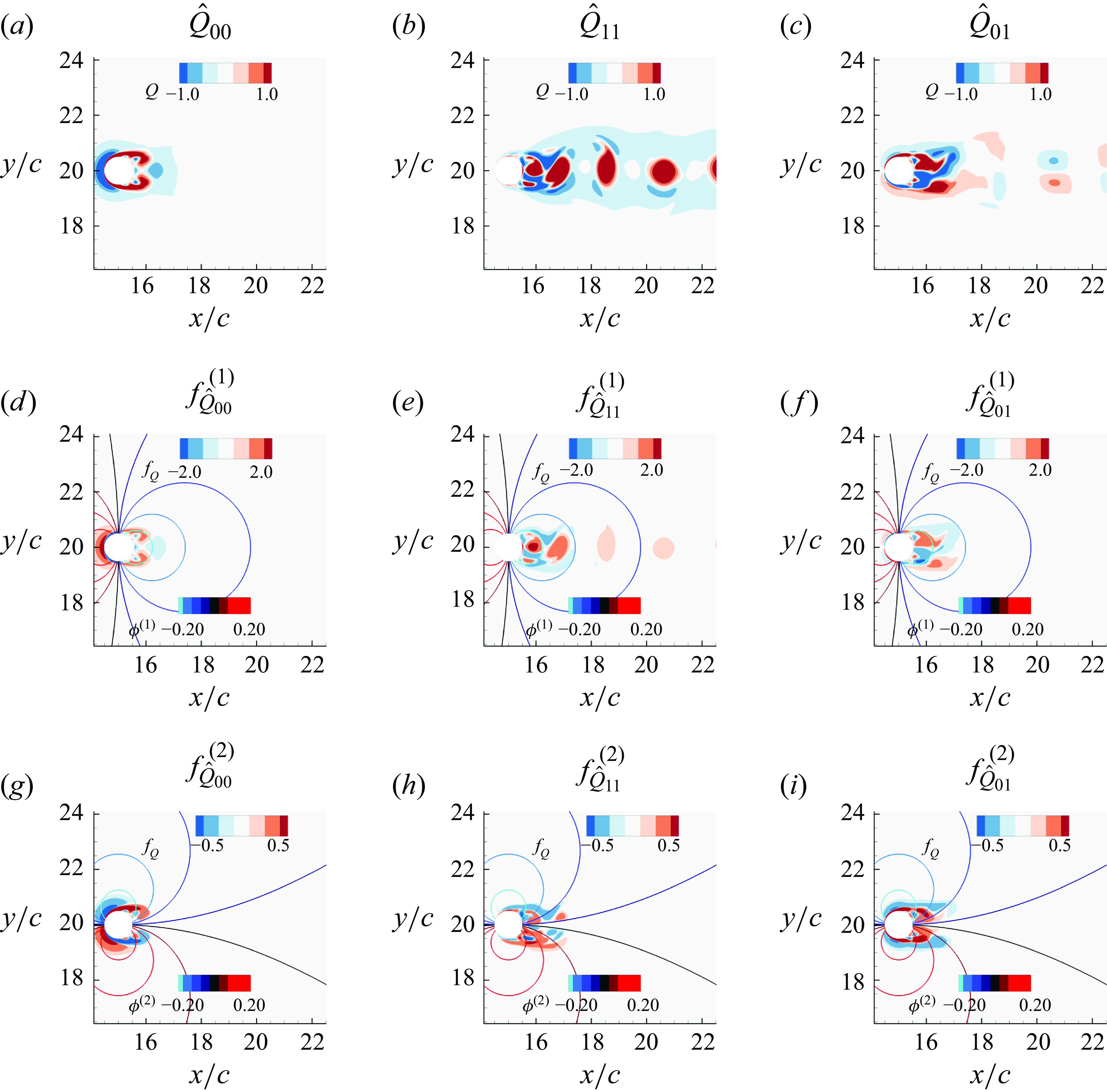
Figure 4. Force partitioning based on Reynolds decomposition of the velocity field for the cylinder flow. Contours of
 $Q$
for (a) the mean flow, (b) the fluctuating component, and (c) the interaction of the mean flow with the fluctuating component. Contours of the vortex-induced drag force density
$Q$
for (a) the mean flow, (b) the fluctuating component, and (c) the interaction of the mean flow with the fluctuating component. Contours of the vortex-induced drag force density
 $f^{(1)}_Q$
and
$f^{(1)}_Q$
and
 $\phi ^{(1)}$
corresponding to (d) the mean flow, (e) the fluctuating component, and (f) the interaction of the mean flow with the fluctuating component. Contours of the vortex-induced lift force density
$\phi ^{(1)}$
corresponding to (d) the mean flow, (e) the fluctuating component, and (f) the interaction of the mean flow with the fluctuating component. Contours of the vortex-induced lift force density
 $f^{(2)}_Q$
and
$f^{(2)}_Q$
and
 $\phi ^{(2)}$
corresponding to (g) the mean flow, (h) the fluctuating component, and (i) the interaction of the mean flow with the fluctuating component.
$\phi ^{(2)}$
corresponding to (g) the mean flow, (h) the fluctuating component, and (i) the interaction of the mean flow with the fluctuating component.
Figures 4(d–f) show the contours of vortex-induced drag force density
 $f_{\hat {Q}_{mn}}^{(1)}$
for these modes, along with the line contours of
$f_{\hat {Q}_{mn}}^{(1)}$
for these modes, along with the line contours of
 $\phi ^{(1)}$
, and figures 4(g–i) show the corresponding plots for lift. We note that
$\phi ^{(1)}$
, and figures 4(g–i) show the corresponding plots for lift. We note that
 $\phi ^{(1)}$
is symmetric about the wake centreline, and has high values in the front and rear of the cylinder. Also
$\phi ^{(1)}$
is symmetric about the wake centreline, and has high values in the front and rear of the cylinder. Also
 $\hat {Q}_{00}$
is symmetric about the wake centreline, therefore
$\hat {Q}_{00}$
is symmetric about the wake centreline, therefore
 $f_{\hat {Q}_{00}}^{(1)}$
, which is the product of these two symmetric functions, is also symmetric, and the integral of this function will result in mean drag. Conversely, since
$f_{\hat {Q}_{00}}^{(1)}$
, which is the product of these two symmetric functions, is also symmetric, and the integral of this function will result in mean drag. Conversely, since
 $\phi ^{(2)}$
is anti-symmetric about the wake centreline,
$\phi ^{(2)}$
is anti-symmetric about the wake centreline,
 $f_{\hat {Q}_{00}}^{(2)}$
will be asymmetric about the centreline and will make no net contribution to the mean lift.
$f_{\hat {Q}_{00}}^{(2)}$
will be asymmetric about the centreline and will make no net contribution to the mean lift.
The integrated drag and lift forces generated due to each of these modes are computed according to the mFPM, and the time variation of these components is shown in figure 5. As indicated above, the
 $(0,0)$
mode is found to contribute to the mean drag force. Both the
$(0,0)$
mode is found to contribute to the mean drag force. Both the
 $(1,1)$
and
$(1,1)$
and
 $(0,1)$
modes contribute to the fluctuation in the drag. The total of these three modes is slightly less than the total pressure drag calculated directly from the integration of the pressure on the surface, and this is because beyond
$(0,1)$
modes contribute to the fluctuation in the drag. The total of these three modes is slightly less than the total pressure drag calculated directly from the integration of the pressure on the surface, and this is because beyond
 $F_Q$
, the
$F_Q$
, the
 $F_\mu$
component (see (2.5)) also makes a small but non-negligible contribution to the mean drag for this low Reynolds number flow.
$F_\mu$
component (see (2.5)) also makes a small but non-negligible contribution to the mean drag for this low Reynolds number flow.
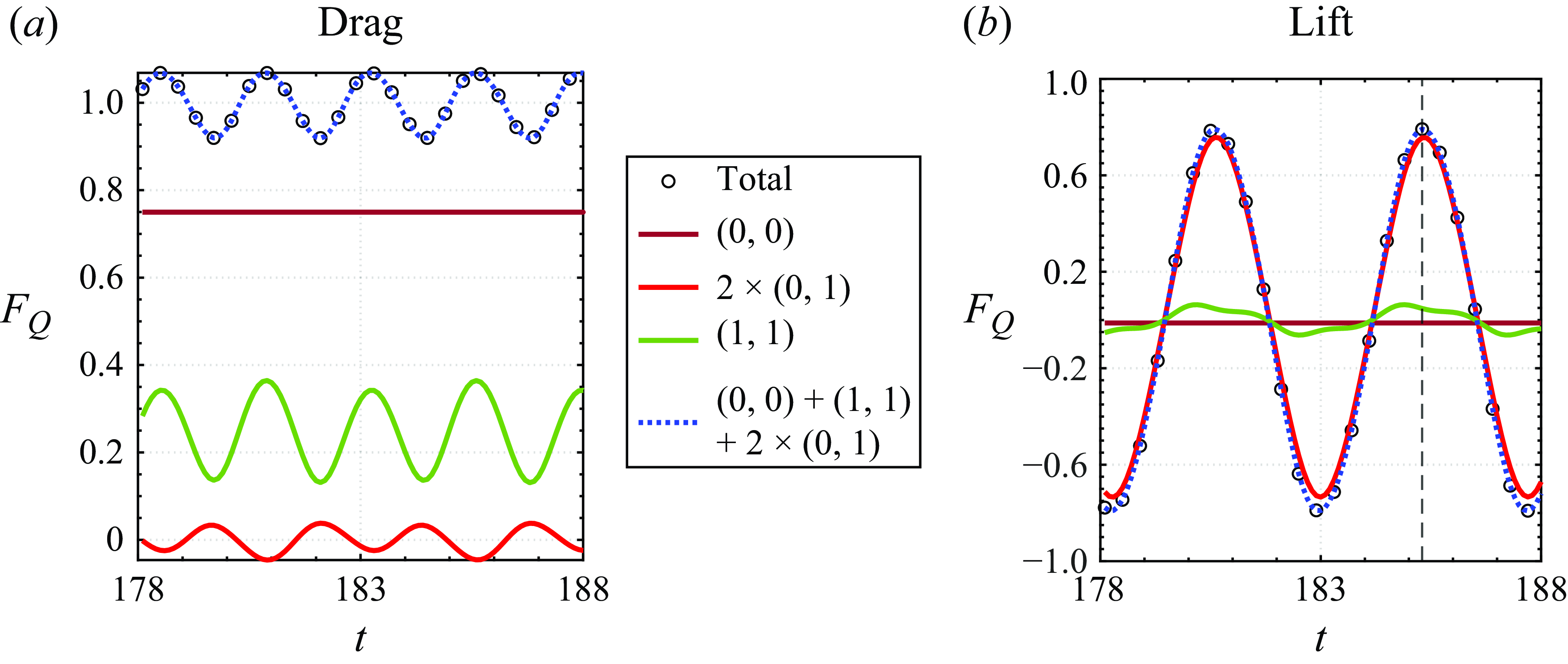
Figure 5. Temporal variation of the non-dimensional vortex-induced (a) drag force (
 $F_Q^{(1)}$
) and (b) lift force (
$F_Q^{(1)}$
) and (b) lift force (
 $F_Q^{(2)}$
) obtained from the Reynolds decomposition of the velocity field of the circular cylinder. The force for all the circular cylinder cases is normalised using the force coefficient (
$F_Q^{(2)}$
) obtained from the Reynolds decomposition of the velocity field of the circular cylinder. The force for all the circular cylinder cases is normalised using the force coefficient (
 $0.5\rho U_\infty ^2 d$
), and the time is normalised using the flow time scale (
$0.5\rho U_\infty ^2 d$
), and the time is normalised using the flow time scale (
 $d/U_\infty$
). The dashed vertical line in (b) shows the time instance where all contour plots for the circular cylinder are shown.
$d/U_\infty$
). The dashed vertical line in (b) shows the time instance where all contour plots for the circular cylinder are shown.
The lift is of particular importance here since it experiences large fluctuations that serve as the dominant source of aeroacoustic noise. As expected, the symmetric mean mode
 $(0,0)$
does not generate any lift. Interestingly, however, we observe that while the fluctuation mode
$(0,0)$
does not generate any lift. Interestingly, however, we observe that while the fluctuation mode
 $\boldsymbol{u}_1$
represents all of the velocity and vorticity fluctuations in the flow, this mode by itself contributes very little to the fluctuation in the lift force. Indeed, the variance of the
$\boldsymbol{u}_1$
represents all of the velocity and vorticity fluctuations in the flow, this mode by itself contributes very little to the fluctuation in the lift force. Indeed, the variance of the
 ${F}^{(2)}_{\hat {Q}_{11}}$
force component is only approximately 0.53 % of the variance in the total lift. The only remaining modal contribution is the inter-modal component
${F}^{(2)}_{\hat {Q}_{11}}$
force component is only approximately 0.53 % of the variance in the total lift. The only remaining modal contribution is the inter-modal component
 $2{F}^{(2)}_{\hat {Q}_{01}}$
, which is the interaction of the fluctuation mode with the mean mode. As shown in figure 5, this component actually provides the overwhelming majority (86.44 %) of the variance in the lift force. Thus the velocity mode that corresponds to the largest variation in the velocity field, i.e.
$2{F}^{(2)}_{\hat {Q}_{01}}$
, which is the interaction of the fluctuation mode with the mean mode. As shown in figure 5, this component actually provides the overwhelming majority (86.44 %) of the variance in the lift force. Thus the velocity mode that corresponds to the largest variation in the velocity field, i.e.
 $\boldsymbol{u}_1$
, generates very little effect on the forces by itself. However, combined with the mean mode, it generates almost all the variation in the lift force. Thus with regard to the lift force induced on the body, the mean mode acts as an ‘amplifier’ for the higher
$\boldsymbol{u}_1$
, generates very little effect on the forces by itself. However, combined with the mean mode, it generates almost all the variation in the lift force. Thus with regard to the lift force induced on the body, the mean mode acts as an ‘amplifier’ for the higher
 $\boldsymbol{u}_1$
mode. This general observation will carry through for other modal decompositions as well. Finally, we note that the sum of all these modal components very slightly under-predicts the total pressure-induced lift force obtained directly from the integration of the pressure on the body. This difference is attributable to the viscous diffusion-induced pressure force
$\boldsymbol{u}_1$
mode. This general observation will carry through for other modal decompositions as well. Finally, we note that the sum of all these modal components very slightly under-predicts the total pressure-induced lift force obtained directly from the integration of the pressure on the body. This difference is attributable to the viscous diffusion-induced pressure force
 $F_\mu$
, and highlights the fact that even at these relatively low Reynolds numbers,
$F_\mu$
, and highlights the fact that even at these relatively low Reynolds numbers,
 $F_\mu$
is very small, therefore the vortex-induced force (
$F_\mu$
is very small, therefore the vortex-induced force (
 $F_\mu$
) provides an accurate estimate of the total pressure-induced force.
$F_\mu$
) provides an accurate estimate of the total pressure-induced force.
Figure 6 shows the directivity field of the sound associated with these modes. As expected from the modal contributions to drag and lift, we find that mode
 $(1,1)$
, which is the dominant mode in the velocity variation, makes only a small contribution to the sound field. On the other hand, the dominant contribution to the sound field comes from the mode
$(1,1)$
, which is the dominant mode in the velocity variation, makes only a small contribution to the sound field. On the other hand, the dominant contribution to the sound field comes from the mode
 $(0,1)$
. Thus the results from even a simple Reynolds decomposition of a relatively low Reynolds number flow are counterintuitive in that the mode most responsible for the variation in the flow field by itself does not account for the dominant variation in the surface pressure and the generation of the noise. This is because the quantity
$(0,1)$
. Thus the results from even a simple Reynolds decomposition of a relatively low Reynolds number flow are counterintuitive in that the mode most responsible for the variation in the flow field by itself does not account for the dominant variation in the surface pressure and the generation of the noise. This is because the quantity
 $Q$
on which the surface force is directly dependent is a nonlinear ‘observable’ and therefore encodes nonlinear interactions in the modes. We explore this next via a POD of this flow.
$Q$
on which the surface force is directly dependent is a nonlinear ‘observable’ and therefore encodes nonlinear interactions in the modes. We explore this next via a POD of this flow.
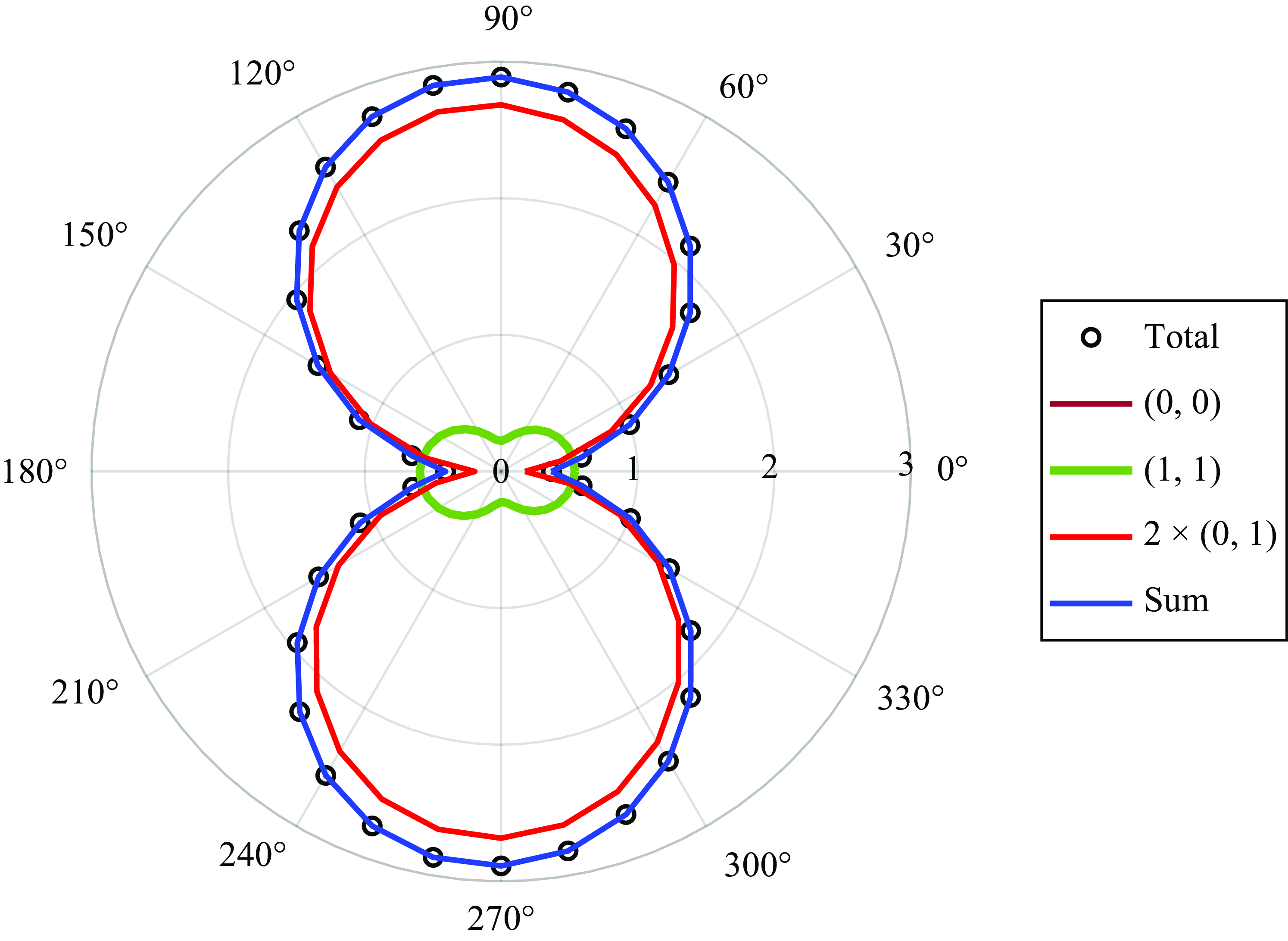
Figure 6. Sound directivity plot based on modal force partitioning applied to the Reynolds decomposition of the velocity field for the circular cylinder flow, showing directivity. The directivity shows
 $p'_{rms}\times 10^{-5}$
, corresponding to surface Mach number 0.1, and is computed at distance
$p'_{rms}\times 10^{-5}$
, corresponding to surface Mach number 0.1, and is computed at distance
 $50d$
.
$50d$
.
3.1.2. Proper orthogonal decomposition
We now apply POD to the flow field of the circular cylinder, and while the mean mode remains the same as that for Reynolds decomposition, the POD procedure partitions the fluctuation component into multiple POD modes (in this case, there are 120 total POD modes). We further note that seven modes (in addition to the mean mode) are required to reconstruct 98 % of the flow field.
To investigate the spatial structures of the modal flow fields, we examined here the spatial eigenvector
 $U\Sigma$
for each POD mode. The vorticities associated with the first four POD modes, which together constitute 99.9 % of the total variation in the flow, are plotted in figures 7(a–d). The symmetry properties of the flow about the wake centreline have important implications for the generation of forces on the body. A velocity field that is reflectionally symmetric about the wake centreline will generate drag but no lift, and a reflectionally anti-symmetric velocity field generates lift but no drag. These properties extend to the POD modes as well. In this regard, we note that Mode-1 is strictly symmetric across the wake centreline, with alternating vortex structures aligned along the wake centreline. Mode-2 and Mode-3, on the other hand, have a strong anti-symmetric topology in the near wake, but transition to a more symmetric configuration in the downstream region. Mode-4 is different from the other modes in that it has a bifurcating topology in the wake and is anti-symmetric in the near wake as well as downstream wake regions. However, force partitioning connects the pressure forces to the
$U\Sigma$
for each POD mode. The vorticities associated with the first four POD modes, which together constitute 99.9 % of the total variation in the flow, are plotted in figures 7(a–d). The symmetry properties of the flow about the wake centreline have important implications for the generation of forces on the body. A velocity field that is reflectionally symmetric about the wake centreline will generate drag but no lift, and a reflectionally anti-symmetric velocity field generates lift but no drag. These properties extend to the POD modes as well. In this regard, we note that Mode-1 is strictly symmetric across the wake centreline, with alternating vortex structures aligned along the wake centreline. Mode-2 and Mode-3, on the other hand, have a strong anti-symmetric topology in the near wake, but transition to a more symmetric configuration in the downstream region. Mode-4 is different from the other modes in that it has a bifurcating topology in the wake and is anti-symmetric in the near wake as well as downstream wake regions. However, force partitioning connects the pressure forces to the
 $Q$
-field, and it is therefore the symmetry properties of the
$Q$
-field, and it is therefore the symmetry properties of the
 $Q$
-field that matter ultimately. Figures 7(e–h) show the
$Q$
-field that matter ultimately. Figures 7(e–h) show the
 $Q$
-fields corresponding to these modes, and we note that
$Q$
-fields corresponding to these modes, and we note that
 $Q_{11}$
is extremely symmetric and other modes (
$Q_{11}$
is extremely symmetric and other modes (
 $Q_{22}$
,
$Q_{22}$
,
 $Q_{33}$
and
$Q_{33}$
and
 $Q_{44}$
) are also mostly symmetric in the near wake. Thus we expect that none of these modes will make any significant contributions to the lift, but could make contributions to the drag force. Inter-modal interactions are also important, and we show
$Q_{44}$
) are also mostly symmetric in the near wake. Thus we expect that none of these modes will make any significant contributions to the lift, but could make contributions to the drag force. Inter-modal interactions are also important, and we show
 $Q$
-fields for two such modes,
$Q$
-fields for two such modes,
 $(0,1)$
and
$(0,1)$
and
 $(0,3)$
. We note that
$(0,3)$
. We note that
 $\hat {Q}_{01}$
is precisely anti-symmetric. Inter-modal interactions between symmetric modes will also generate symmetric
$\hat {Q}_{01}$
is precisely anti-symmetric. Inter-modal interactions between symmetric modes will also generate symmetric
 $Q$
-fields, but beyond this, it is not readily apparent how to predict the symmetry properties of the
$Q$
-fields, but beyond this, it is not readily apparent how to predict the symmetry properties of the
 $Q$
-field corresponding to other complex inter-modal interactions such as for
$Q$
-field corresponding to other complex inter-modal interactions such as for
 $(0,3)$
.
$(0,3)$
.
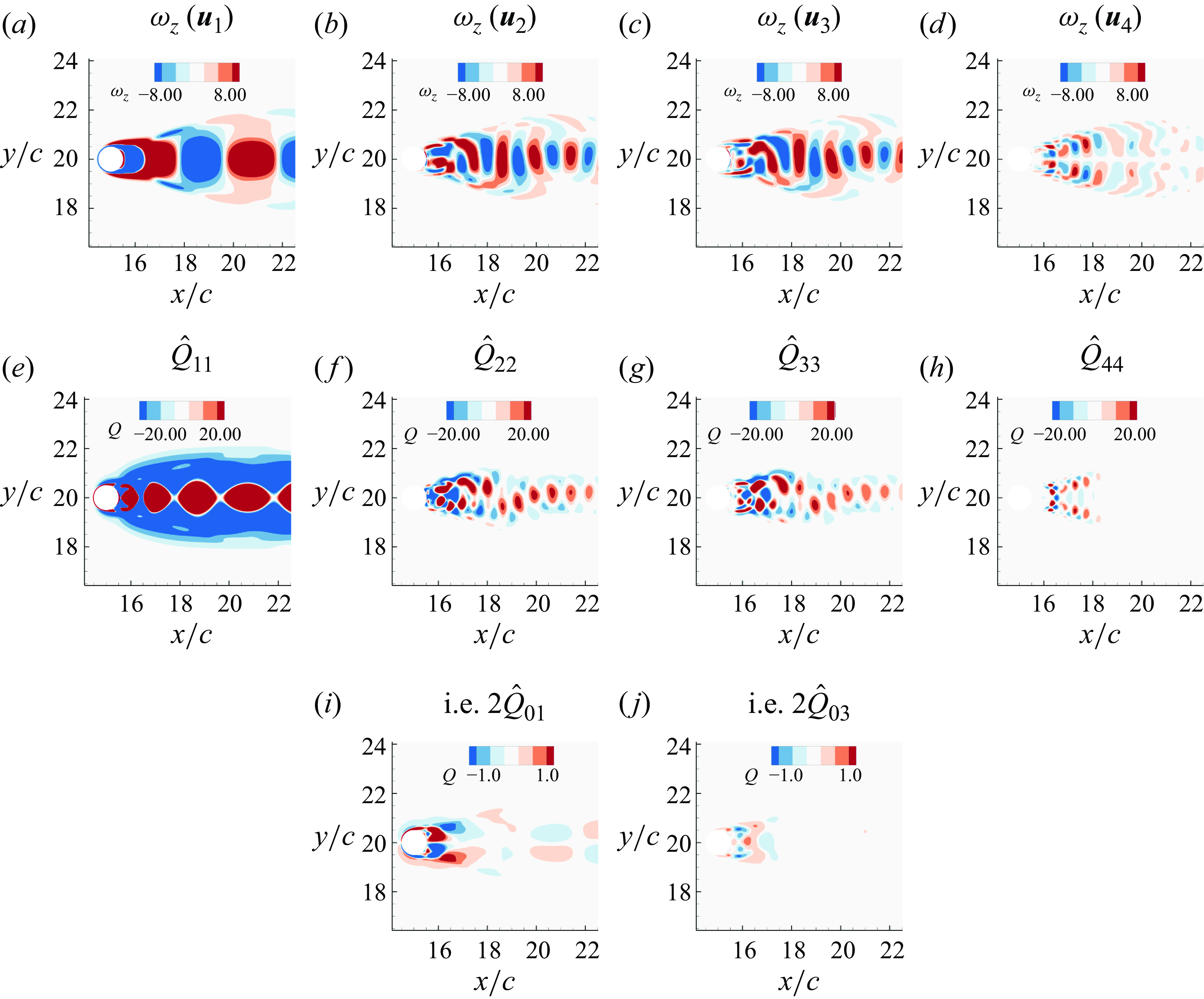
Figure 7. The POD applied to the velocity for circular cylinder flow. Spanwise vorticity shown for the spatial eigenvector (
 $U\Sigma$
) corresponding to (a) Mode-1, (b) Mode-2, (c) Mode-3 and (d) Mode-4. The
$U\Sigma$
) corresponding to (a) Mode-1, (b) Mode-2, (c) Mode-3 and (d) Mode-4. The
 $Q$
-fields are shown for the spatial eigenvectors (
$Q$
-fields are shown for the spatial eigenvectors (
 $U\Sigma$
) corresponding to (e) Mode-1, (f) Mode-2, (g) Mode-3 and (h) Mode-4.The
$U\Sigma$
) corresponding to (e) Mode-1, (f) Mode-2, (g) Mode-3 and (h) Mode-4.The
 $Q$
-fields corresponding to the interaction between the mean mode and POD modes are shown for (i) Mode-0 and (j) Mode-3.
$Q$
-fields corresponding to the interaction between the mean mode and POD modes are shown for (i) Mode-0 and (j) Mode-3.
Figure 8 shows the contribution of the various POD modes, including the contributions of the inter-modal interactions to the pressure drag and lift. We show only those components that make a noticeable contribution to the force in question. The mean drag is connected with the (0,0) mode as expected. The time variation in the drag force is dominated by the symmetric (1,1) mode, but the inter-modal interactions (0,2) and (0,3) also make a small but noticeable contribution to the drag variation. For the lift, the symmetric modes, including (0,0), (1,1), (2,2), (3,3) and (4,4), do not make any contribution to the lift. However, mode (0,1), which as shown earlier, is purely anti-symmetric in
 $Q$
, makes a dominant contribution to the lift force variation. The mode (1,2) makes a very small (barely noticeable) contribution to the lift variation, and other than that, all other contributions are negligible.
$Q$
, makes a dominant contribution to the lift force variation. The mode (1,2) makes a very small (barely noticeable) contribution to the lift variation, and other than that, all other contributions are negligible.
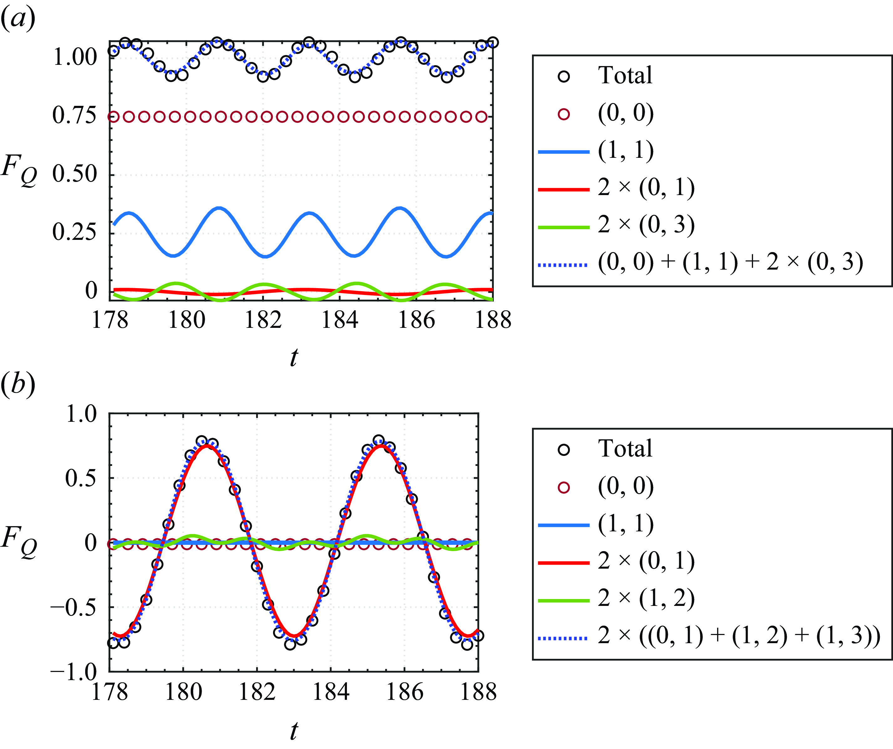
Figure 8. Non-dimensional vortex-induced forces obtained for modes resulting from POD applied to the velocity field (a) drag force (
 $F_Q^{(1)}$
) and (b) lift force (
$F_Q^{(1)}$
) and (b) lift force (
 $F_Q^{(2)}$
). The plot shows intra-modal and inter-modal interactions.
$F_Q^{(2)}$
). The plot shows intra-modal and inter-modal interactions.
The aerodynamic sound generated by these fluctuating forces is computed by the method described in § 2.4. The flow Mach number is assumed to be
 $M=0.1$
, and the root mean square (RMS) sound pressure shown in figure 9(a) is computed at a distance of 50 diameters below the cylinder. The bars show the integrated sound pressure resulting from the intra-modal ((1,1), (2,2), …) and inter-modal ((0,1), (1,2), …) interactions. The largest component of the pressure force fluctuation is that generated in the lift by the interaction of Mode-0 (mean) and Mode-1, and we see that this interaction captures most of the aeroacoustic noise in the form of a dipole oriented in the vertical direction. Mode-1, which generates the vast majority of the drag oscillations, also generates a small contribution as a dipole oriented in the horizontal direction. Very small contributions to noise are also generated by the interaction of Mode-1 with Mode-2 and Mode-3.
$M=0.1$
, and the root mean square (RMS) sound pressure shown in figure 9(a) is computed at a distance of 50 diameters below the cylinder. The bars show the integrated sound pressure resulting from the intra-modal ((1,1), (2,2), …) and inter-modal ((0,1), (1,2), …) interactions. The largest component of the pressure force fluctuation is that generated in the lift by the interaction of Mode-0 (mean) and Mode-1, and we see that this interaction captures most of the aeroacoustic noise in the form of a dipole oriented in the vertical direction. Mode-1, which generates the vast majority of the drag oscillations, also generates a small contribution as a dipole oriented in the horizontal direction. Very small contributions to noise are also generated by the interaction of Mode-1 with Mode-2 and Mode-3.
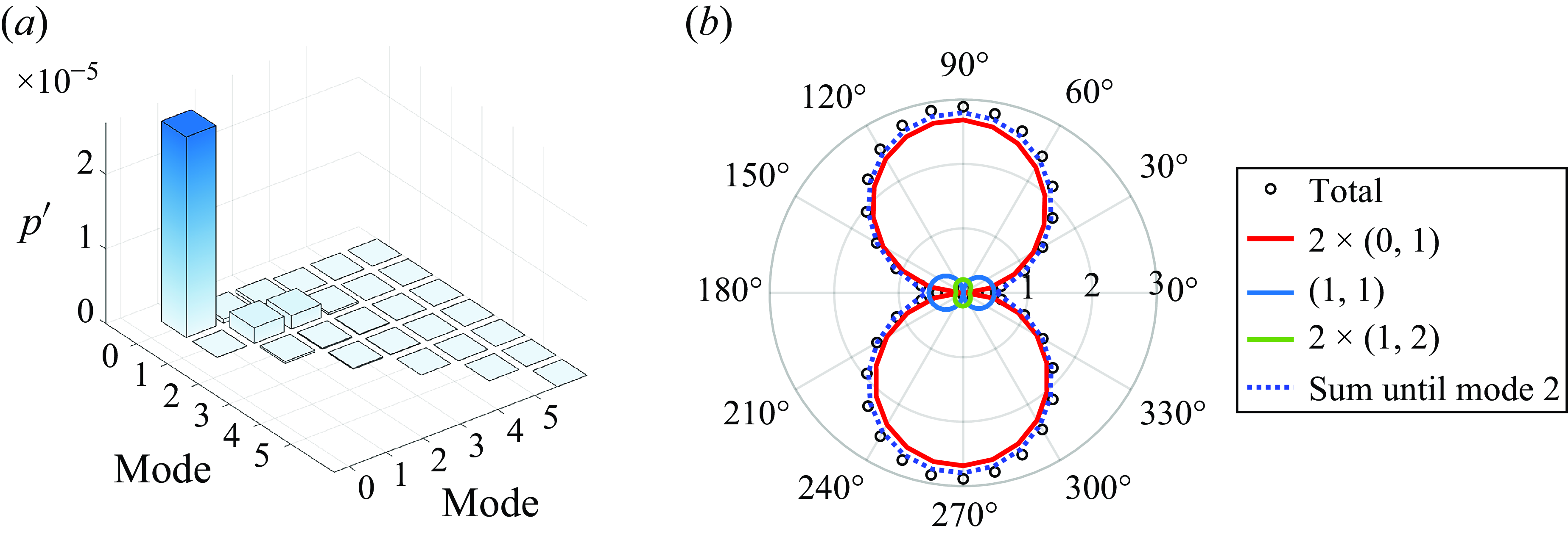
Figure 9. The aeroacoustic noise, calculated at a distance
 $50d$
relative to the centre of the cylinder, and corresponding to Mach number 0.1 for the POD of the velocity field of the circular cylinder flow, shows (a) the RMS of sound pressure level at location
$50d$
relative to the centre of the cylinder, and corresponding to Mach number 0.1 for the POD of the velocity field of the circular cylinder flow, shows (a) the RMS of sound pressure level at location
 $(x=0,y=-50d)$
for the first six modal interactions, and (b) the directivity (
$(x=0,y=-50d)$
for the first six modal interactions, and (b) the directivity (
 $p'_{rms}\times 10^{-5}$
) shown for the dominant modes and their interactions.
$p'_{rms}\times 10^{-5}$
) shown for the dominant modes and their interactions.
We make two observations from these plots. First, Mode-1, the POD mode that captures most of the fluctuation in the velocity associated with the Karman vortex shedding, does not generate by itself the dominant component of the aeroacoustic noise. Rather, it is the inter-modal interaction between Mode-0 and Mode-1 that is responsible for most of the noise. Second, as shown from the bar chart of the sound pressure contribution, the appearance of (0,1) and other inter-modal interactions makes it difficult to pinpoint individual modes that are particularly important for noise generation. As will be shown later in the paper, this complexity increases very rapidly with increasing Reynolds number, since these flows have a wide range of modes with substantial energy.
3.1.3. Modal decomposition of
$Q$

Motivated by the above complication, we propose to examine modal decompositions of the
 $Q$
-field as a way to directly access the features/modes in the flow that are responsible for the generation of pressure forces on the body. It is expected that this will circumvent the need to consider inter-modal interactions and result in a modal decomposition approach that more directly targets pressure forces.
$Q$
-field as a way to directly access the features/modes in the flow that are responsible for the generation of pressure forces on the body. It is expected that this will circumvent the need to consider inter-modal interactions and result in a modal decomposition approach that more directly targets pressure forces.
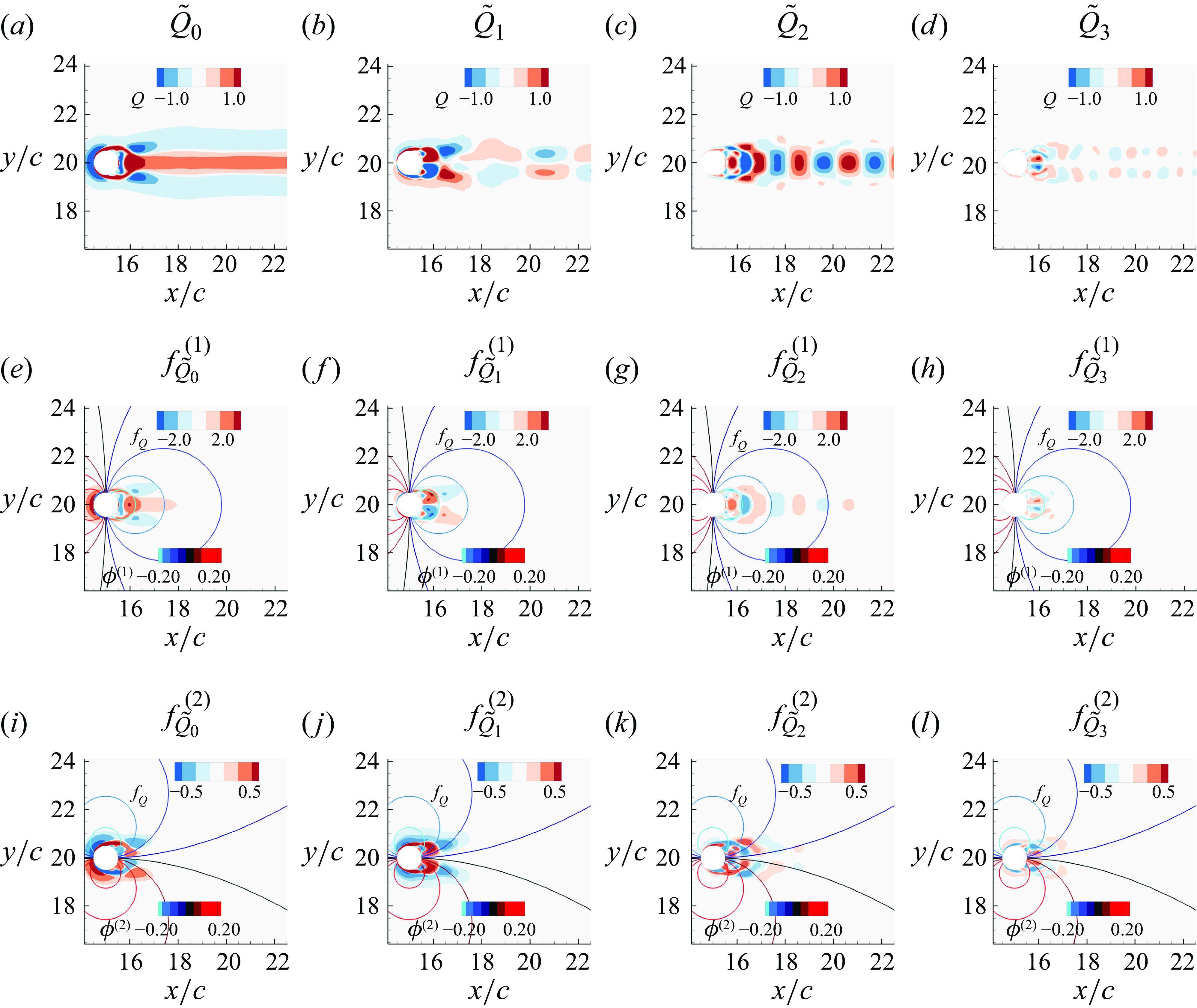
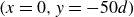
Figure 10. Modal force partitioning based on POD of
 $Q$
-fields. Contours of
$Q$
-fields. Contours of
 $Q$
for (a) the mean mode (i.e.
$Q$
for (a) the mean mode (i.e.
 $\tilde {Q}_{0}$
), (b) Mode-1 (i.e.
$\tilde {Q}_{0}$
), (b) Mode-1 (i.e.
 $\tilde {Q}_{1}$
), (c) Mode-2 (i.e.
$\tilde {Q}_{1}$
), (c) Mode-2 (i.e.
 $\tilde {Q}_{2}$
), and (d) Mode-3 (i.e.
$\tilde {Q}_{2}$
), and (d) Mode-3 (i.e.
 $\tilde {Q}_{3}$
). Contours of vortex-induced drag force density
$\tilde {Q}_{3}$
). Contours of vortex-induced drag force density
 $f^{(1)}_Q$
and
$f^{(1)}_Q$
and
 $\phi ^{(1)}$
corresponding to (e) the mean mode, (f) Mode-1, (g) Mode-2 and (h) Mode-3. Contours of vortex-induced lift force density
$\phi ^{(1)}$
corresponding to (e) the mean mode, (f) Mode-1, (g) Mode-2 and (h) Mode-3. Contours of vortex-induced lift force density
 $f^{(2)}_Q$
and
$f^{(2)}_Q$
and
 $\phi ^{(2)}$
corresponding to (i) the mean mode, (j) Mode-1, (k) Mode-2 and (l) Mode-3.
$\phi ^{(2)}$
corresponding to (i) the mean mode, (j) Mode-1, (k) Mode-2 and (l) Mode-3.
In this approach,
 $Q$
-fields are computed as functions of space and time from the total velocity, and then subject to modal analysis. Then
$Q$
-fields are computed as functions of space and time from the total velocity, and then subject to modal analysis. Then
 $Q$
would be represented as a sum of
$Q$
would be represented as a sum of
 $N$
modes as
$N$
modes as
 \begin{equation} Q(\boldsymbol{x},t) = \tilde {Q}_0 (\boldsymbol{x}) + \tilde {Q}_1(\boldsymbol{x},t) +\tilde {Q}_2(\boldsymbol{x},t) +\cdots + \tilde {Q}_N(\boldsymbol{x},t), \end{equation}
where
 $\tilde {Q}_m$
is the
$\tilde {Q}_m$
is the
 $m$
th mode of the
$m$
th mode of the
 $Q$
-field. The force induced by this mode is given by
$Q$
-field. The force induced by this mode is given by
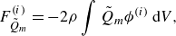 \begin{equation} F_{\tilde {Q}_m}^{(i)}=-2\rho \int \tilde {Q}_{m}\phi ^{(i)}\, {\rm d}V , \end{equation}
and the corresponding vortex-induced noise is given by
 \begin{equation} p'_{\tilde {Q}_m}=\frac {\boldsymbol{r}}{4\unicode{x03C0} r^2}\left [\left (\frac {1}{c} \frac {\partial }{\partial t}+\frac {1}{r}\right )\boldsymbol{\cdot} \boldsymbol{F}_{\tilde {Q}_m} \right ]_{t-{r}/{c}} . \end{equation}
We apply POD to the
 $Q$
-field, and the first three POD modes are shown in figure 10. Mode-1, shown in figure 10(a), is anti-symmetric about the wake centreline, and the topology of the modes is indicative of the alternative vortex shedding in the near wake and the large oscillation of the lateral velocity in the wake. Mode-2 and Mode-3 are symmetric and anti-symmetric, respectively. Mode-2, in particular, is comparable in magnitude to Mode-1 and it is indicative of the symmetric fluctuations in streamwise velocity generated by the vortices shed in the wake. Due to these symmetry properties, we expect that while Mode-1 and Mode-3 will contribute to lift only, Mode-2 will contribute only to drag. The corresponding contour plots of
$Q$
-field, and the first three POD modes are shown in figure 10. Mode-1, shown in figure 10(a), is anti-symmetric about the wake centreline, and the topology of the modes is indicative of the alternative vortex shedding in the near wake and the large oscillation of the lateral velocity in the wake. Mode-2 and Mode-3 are symmetric and anti-symmetric, respectively. Mode-2, in particular, is comparable in magnitude to Mode-1 and it is indicative of the symmetric fluctuations in streamwise velocity generated by the vortices shed in the wake. Due to these symmetry properties, we expect that while Mode-1 and Mode-3 will contribute to lift only, Mode-2 will contribute only to drag. The corresponding contour plots of
 $f_Q$
for drag and lift are shown below these plots. The multiplication of
$f_Q$
for drag and lift are shown below these plots. The multiplication of
 $Q$
with these influence fields tends to diminish the influence of distant features. Furthermore, while
$Q$
with these influence fields tends to diminish the influence of distant features. Furthermore, while
 $\phi ^{(1)}$
, due to its symmetric nature, tends to emphasise the vortex structures in the stagnation and wake regions, anti-symmetric
$\phi ^{(1)}$
, due to its symmetric nature, tends to emphasise the vortex structures in the stagnation and wake regions, anti-symmetric
 $\phi ^{(2)}$
diminishes the influence of the structures in these regions, and emphasises the features above the cylinder.
$\phi ^{(2)}$
diminishes the influence of the structures in these regions, and emphasises the features above the cylinder.
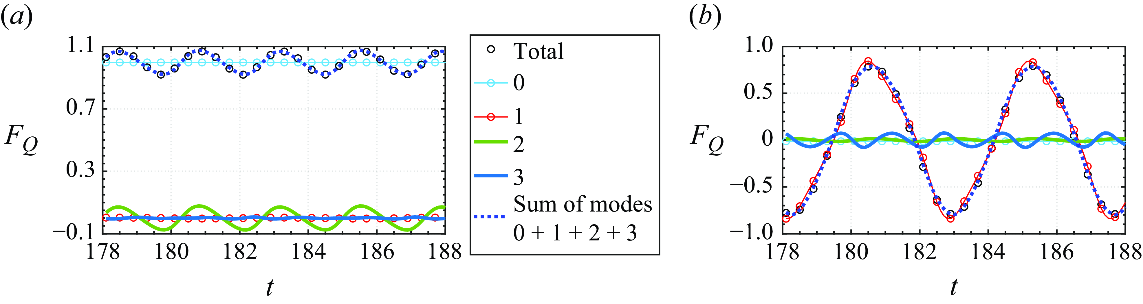
Figure 11. Temporal variation of the non-dimensional vortex-induced (a) drag force (
 $F_Q^{(1)}$
) and (b) lift force (
$F_Q^{(1)}$
) and (b) lift force (
 $F_Q^{(2)}$
) for the dominant POD modes obtained from application of POD applied to the
$F_Q^{(2)}$
) for the dominant POD modes obtained from application of POD applied to the
 $Q$
-field of the circular cylinder flow.
$Q$
-field of the circular cylinder flow.
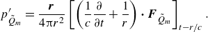
Figures 11(a) and 11(b) show plots of vortex-induced drag and lift force versus time for these modes, respectively. With respect to drag, we note that Mode-0 provides the mean drag, and Mode-2 provides most of the time variation in this quantity. Mode-1 and Mode-3, which are anti-symmetric modes, do not provide any contribution to drag. With regard to lift, Mode-1 and Mode-3 provide almost all of the time variation in this quantity, with Mode-1 having a high amplitude, and Mode-3 having a much lower amplitude and higher frequency (by a factor of 3) compared to Mode-1. The other modes do not provide any significant contribution to drag.
Figure 12(a) shows the normalised values of the eigenvalues for the POD modes of
 $Q$
. The vortex-induced force is calculated for each of the POD modes of the
$Q$
. The vortex-induced force is calculated for each of the POD modes of the
 $Q$
-field, and the corresponding values normalised by the vortex-induced lift force value of the first mode are shown using the solid black line. We see from the peaks that the important modes related to the lift force are Mode-1 and Mode-3.
$Q$
-field, and the corresponding values normalised by the vortex-induced lift force value of the first mode are shown using the solid black line. We see from the peaks that the important modes related to the lift force are Mode-1 and Mode-3.
Figure 12. Application of POD applied to the
 $Q$
-field for the circular cylinder showing (a) normalised eigenvalues (with 12 modes required to reconstruct 98 % of the
$Q$
-field for the circular cylinder showing (a) normalised eigenvalues (with 12 modes required to reconstruct 98 % of the
 $Q$
-field) and vortex-induced total force (
$Q$
-field) and vortex-induced total force (
 $\sqrt {(F_Q^{(1)})^2+(F_Q^{(2)})^2}$
), and (b) the sound directivity (
$\sqrt {(F_Q^{(1)})^2+(F_Q^{(2)})^2}$
), and (b) the sound directivity (
 $p'_{rms}\times 10^{-5}$
). The values were calculated at a distance
$p'_{rms}\times 10^{-5}$
). The values were calculated at a distance
 $50d$
away, and correspond to surface Mach number 0.1.
$50d$
away, and correspond to surface Mach number 0.1.
Figure 12(b) shows the directivity plots of the aeroacoustic sound associated with these modes. We find that Mode-1 generates the vast majority of the sound, and this in the form of a vertically oriented dipole. Mode-2 and Mode-3 provide much lower but similar levels of overall sound intensities, but while Mode-2 sound is a dipole directed in the horizontal direction, Mode-3 sound is a dipole in the vertical direction.
The above discussion shows that a direct decomposition of
 $Q$
generates a simpler description of the influence of the decomposed modes on the pressure forces and the induced sounds. This is due primarily to the elimination of complex inter-modal interactions that are generated in the
$Q$
generates a simpler description of the influence of the decomposed modes on the pressure forces and the induced sounds. This is due primarily to the elimination of complex inter-modal interactions that are generated in the
 $Q$
-field when the modal decomposition is based on the velocity field. We also note that for this simple circular cylinder case, the modes obtained from the decomposition of
$Q$
-field when the modal decomposition is based on the velocity field. We also note that for this simple circular cylinder case, the modes obtained from the decomposition of
 $Q$
exhibit useful symmetries (as in figure 10) that are connected with their influence on the vector pressure forces induced on the body. Based on this, it is clear that the application of modal force partitioning is particularly useful when paired with a direct decomposition of
$Q$
exhibit useful symmetries (as in figure 10) that are connected with their influence on the vector pressure forces induced on the body. Based on this, it is clear that the application of modal force partitioning is particularly useful when paired with a direct decomposition of
 $Q$
, and we focus primarily on this approach for the remaining cases in this paper.
$Q$
, and we focus primarily on this approach for the remaining cases in this paper.
We also simulated and decomposed the
 $Q$
-field of the circular cylinder at
$Q$
-field of the circular cylinder at
 $Re=150$
, keeping other parameters consistent with the
$Re=150$
, keeping other parameters consistent with the
 $Re=300$
case. We observed that the modes of the resulting decomposition at this lower Reynolds number exhibit a noise directivity pattern similar to the
$Re=300$
case. We observed that the modes of the resulting decomposition at this lower Reynolds number exhibit a noise directivity pattern similar to the
 $Re=300$
case shown in figure 12(b). Specifically, Mode-1 and Mode-3 are vertically oriented dipoles, while Mode-2 represents a horizontally oriented dipole. Thus the behaviour is similar despite a factor of two difference in the Reynolds number.
$Re=300$
case shown in figure 12(b). Specifically, Mode-1 and Mode-3 are vertically oriented dipoles, while Mode-2 represents a horizontally oriented dipole. Thus the behaviour is similar despite a factor of two difference in the Reynolds number.
3.2. Flow past an aerofoil at
$Re=2500$

Next, an NACA 0015 aerofoil at a high angle of attack (20
 $^\circ$
) and higher Reynolds number (
$^\circ$
) and higher Reynolds number (
 $Re_c=2500$
, based on the chord (
$Re_c=2500$
, based on the chord (
 $c$
) and the incoming flow velocity (
$c$
) and the incoming flow velocity (
 $U_\infty$
)) is considered, and this provides a greater level of complexity than the low Reynolds number circular cylinder flow. The instantaneous vorticity field for this case is plotted in figure 13(a), which shows shedding of vortices from the leading as well as trailing edges. As will be shown shortly, this flow not only has a dominant cyclic component, but also exhibits significant cycle-to-cycle variations. Thus this flow is a good candidate to demonstrate the application of modal force partitioning to a triple decomposition of a flow.
$U_\infty$
)) is considered, and this provides a greater level of complexity than the low Reynolds number circular cylinder flow. The instantaneous vorticity field for this case is plotted in figure 13(a), which shows shedding of vortices from the leading as well as trailing edges. As will be shown shortly, this flow not only has a dominant cyclic component, but also exhibits significant cycle-to-cycle variations. Thus this flow is a good candidate to demonstrate the application of modal force partitioning to a triple decomposition of a flow.
3.2.1. Triple decomposition of the velocity field
Triple decomposition (Hussain & Reynolds Reference Hussain and Reynolds1970a
) is used to partition the fluctuating component into coherent (
 $\boldsymbol{u}_1$
) and incoherent (
$\boldsymbol{u}_1$
) and incoherent (
 $\boldsymbol{u}_2$
) components, with the flow field interval chosen such that it contains 9 cycles of the coherent wave, with 32 snapshots in each cycle. The flow structures generated by these components via the decomposition of the velocity field are shown in figure 13, and we observe that the coherent component captures the separation of the leading-edge vortex (LEV) and the Karman-like vortex shedding in the wake. The incoherent component captures variations along the periphery of the primary vortices (the LEV and the wake vortices), since these regions are more significantly affected by the chaotic nature of the flow than the cores of the vortices. The vortices seen in the coherent mode are also arranged sequentially in series of anticlockwise vorticity originating from the trailing edge and clockwise vorticity originating from the leading edge, while the vortices shed in incoherent mode appear in thin sheets and in vortex pairs.
$\boldsymbol{u}_2$
) components, with the flow field interval chosen such that it contains 9 cycles of the coherent wave, with 32 snapshots in each cycle. The flow structures generated by these components via the decomposition of the velocity field are shown in figure 13, and we observe that the coherent component captures the separation of the leading-edge vortex (LEV) and the Karman-like vortex shedding in the wake. The incoherent component captures variations along the periphery of the primary vortices (the LEV and the wake vortices), since these regions are more significantly affected by the chaotic nature of the flow than the cores of the vortices. The vortices seen in the coherent mode are also arranged sequentially in series of anticlockwise vorticity originating from the trailing edge and clockwise vorticity originating from the leading edge, while the vortices shed in incoherent mode appear in thin sheets and in vortex pairs.
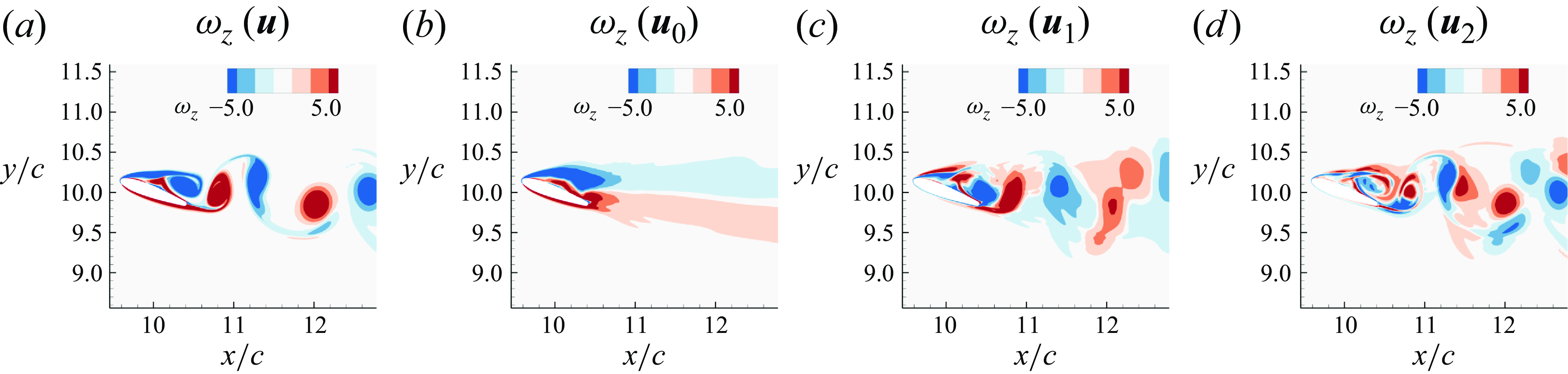
Figure 13. Spanwise vorticity associated with the modes associated with the triple decomposition of the velocity field for the aerofoil flow showing (a) a snapshot of the flow field before decomposition, (b) the mean mode (
 $\boldsymbol{u}_0$
), (c) the coherent mode (
$\boldsymbol{u}_0$
), (c) the coherent mode (
 $\boldsymbol{u}_1$
), and (d) the incoherent mode (
$\boldsymbol{u}_1$
), and (d) the incoherent mode (
 $\boldsymbol{u}_2$
).
$\boldsymbol{u}_2$
).
The contributions of the decomposed flow modes to the aerodynamic sound are obtained by applying the FAPM as described above. The flow Mach number is set to
 $M=0.1$
, and the sound pressure is evaluated at a distance
$M=0.1$
, and the sound pressure is evaluated at a distance
 $57c$
from the aerofoil. The RMS value of sound pressure at a location directly above the aerofoil at distance
$57c$
from the aerofoil. The RMS value of sound pressure at a location directly above the aerofoil at distance
 $57c$
is shown in figure 14(a). As we have seen for the circular cylinder case, the aerodynamic sound is characterised by the intra-modal as well as inter-modal interactions. We find that the interaction between the mean and coherent modes (0,1) generates the strongest dipole sound, but other inter-modal interactions also contribute substantially to the radiated sound. The directivity patterns for the sound generated by modal interactions at distance
$57c$
is shown in figure 14(a). As we have seen for the circular cylinder case, the aerodynamic sound is characterised by the intra-modal as well as inter-modal interactions. We find that the interaction between the mean and coherent modes (0,1) generates the strongest dipole sound, but other inter-modal interactions also contribute substantially to the radiated sound. The directivity patterns for the sound generated by modal interactions at distance
 $57c$
are plotted in figure 14(b), and these also show that the directivities of the inter-modal interactions can be quite distinct.
$57c$
are plotted in figure 14(b), and these also show that the directivities of the inter-modal interactions can be quite distinct.
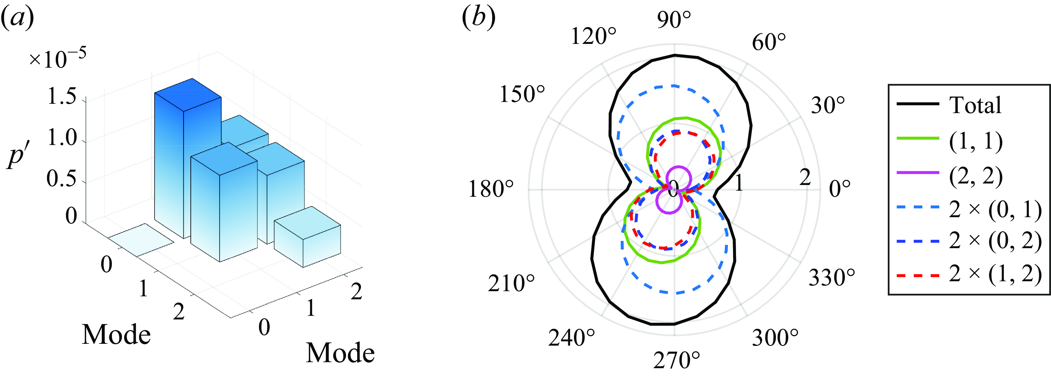
Figure 14. (a) The RMS value of sound pressure calculated at 270
 $^\circ$
and associated with the intra-modal and inter-modal interactions. (b) The corresponding directivity (
$^\circ$
and associated with the intra-modal and inter-modal interactions. (b) The corresponding directivity (
 $p'_{rms}\times 10^{-5}$
) pattern.
$p'_{rms}\times 10^{-5}$
) pattern.
This result reaffirms the observation made for the POD of the cylinder case that if the modal decomposition is applied to the velocity field, then it is not easy to identify the dominant noise modes and the associated flow structures, since they are entangled by inter-modal interactions. This is even more apparent for this aerofoil flow at a higher Reynolds number, since this flow generates substantial energy in the higher mode, resulting in more substantial inter-modal interactions.
3.2.2. Triple decomposition of the
$Q$
-field

As shown in the previous subsubsection, based on the FPM and FAPM formulations, if we decompose the
 $Q$
-field directly, then the issues associated with inter-modal interactions can be avoided. Thus the triple decomposition is now applied directly to the
$Q$
-field directly, then the issues associated with inter-modal interactions can be avoided. Thus the triple decomposition is now applied directly to the
 $Q$
-field. The temporally and spatially varying
$Q$
-field. The temporally and spatially varying
 $Q$
-field is directly decomposed into a mean component (figure 15
b), a coherent part (figure 15
c), and the remaining incoherent part (figure 15
d). The mean flow depicts the vortical structure due to the flow separation over the aerofoil, and the coherent part captures the shedding of LEVs and trailing-edge vortices. The incoherent part shows thin sheets of positive and negative
$Q$
-field is directly decomposed into a mean component (figure 15
b), a coherent part (figure 15
c), and the remaining incoherent part (figure 15
d). The mean flow depicts the vortical structure due to the flow separation over the aerofoil, and the coherent part captures the shedding of LEVs and trailing-edge vortices. The incoherent part shows thin sheets of positive and negative
 $Q$
around the shed vortices, which represent the effect of cycle-to-cycle variations that occur mostly along the periphery of the large vortices as they interact with the other vortices in the flow. Thus modes obtained from the direct decomposition of the
$Q$
around the shed vortices, which represent the effect of cycle-to-cycle variations that occur mostly along the periphery of the large vortices as they interact with the other vortices in the flow. Thus modes obtained from the direct decomposition of the
 $Q$
-field are also amenable to interpretation, which is quite often the key in gaining some insight into these phenomena.
$Q$
-field are also amenable to interpretation, which is quite often the key in gaining some insight into these phenomena.
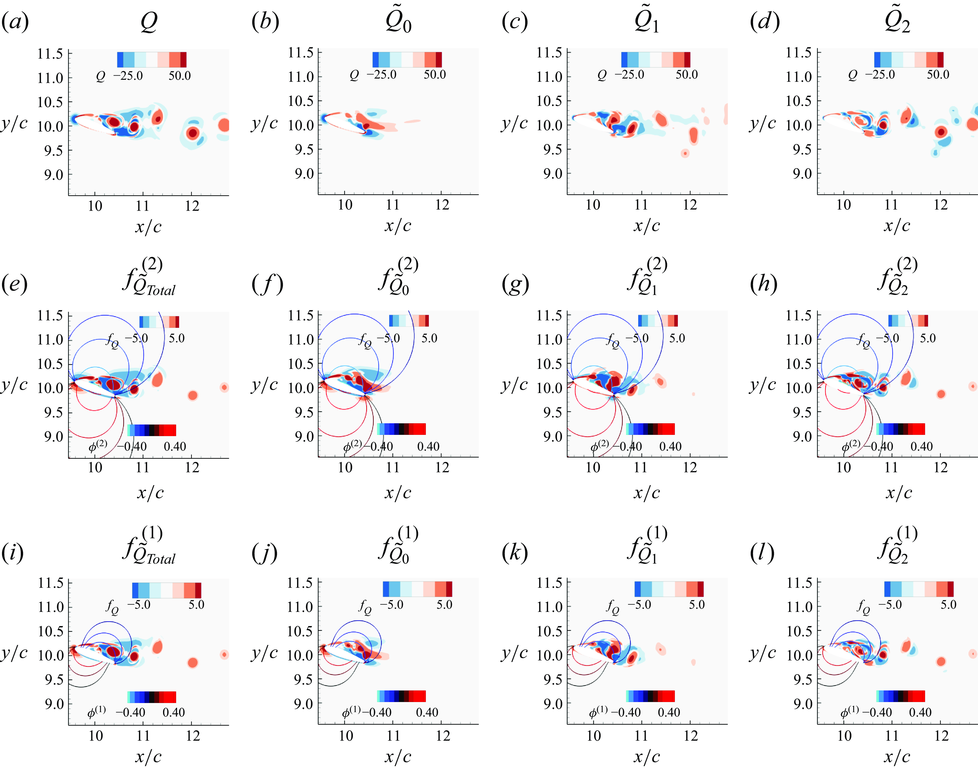
Figure 15. Triple decomposition applied directly to the
 $Q$
-field of the aerofoil showing contours of
$Q$
-field of the aerofoil showing contours of
 $Q$
for (a) a snapshot of the flow, (b) the mean flow, (c) the coherent part of the flow, and (d) the non-coherent part of the flow. (e–h) The corresponding contour plots of vortex-induced lift force density (
$Q$
for (a) a snapshot of the flow, (b) the mean flow, (c) the coherent part of the flow, and (d) the non-coherent part of the flow. (e–h) The corresponding contour plots of vortex-induced lift force density (
 $f_Q^{(2)}$
) and
$f_Q^{(2)}$
) and
 $\phi ^{(2)}$
. (i–l) The corresponding contour plots of vortex-induced drag force density (
$\phi ^{(2)}$
. (i–l) The corresponding contour plots of vortex-induced drag force density (
 $f_Q^{(1)}$
) and
$f_Q^{(1)}$
) and
 $\phi ^{(1)}$
.
$\phi ^{(1)}$
.
The influence fields in the vertical direction (
 $\phi ^{(2)}$
) along with the vortex-induced lift force density are plotted for each mode in figures 15(e–h), and the influence fields in the horizontal direction (
$\phi ^{(2)}$
) along with the vortex-induced lift force density are plotted for each mode in figures 15(e–h), and the influence fields in the horizontal direction (
 $\phi ^{(1)}$
) along with the vortex-induced drag force density are plotted in figures 15(i–l). As noted earlier, the vortical structures near the aerofoil contribute more significantly to the pressure force on the body. For the coherent part, the shedding of the LEV is key to the generation of periodic force fluctuations. The cycle-to-cycle variation of the size and strength of this vortex-induced force is captured by the incoherent mode.
$\phi ^{(1)}$
) along with the vortex-induced drag force density are plotted in figures 15(i–l). As noted earlier, the vortical structures near the aerofoil contribute more significantly to the pressure force on the body. For the coherent part, the shedding of the LEV is key to the generation of periodic force fluctuations. The cycle-to-cycle variation of the size and strength of this vortex-induced force is captured by the incoherent mode.
The time variations of the vortex-induced drag (
 $F_Q^{(1)}$
) and lift (
$F_Q^{(1)}$
) and lift (
 $F_Q^{(2)}$
) forces obtained by applying the FPM with the triple-decomposed
$F_Q^{(2)}$
) forces obtained by applying the FPM with the triple-decomposed
 $Q$
-fields are shown in figure 16, and we see that the total vortex-induced force has a dominant cyclical component; it deviates from a strictly periodic variation, and provides the motivation for the use of a triple decomposition for this case. As expected, the mean mode alone produces the mean vortex-induced drag and lift forces, but it lacks temporal variance and hence is incapable of generating any aeroacoustic sound. The coherent part of the flow (Mode-1) consists of a periodic variation and produces a major portion of the force fluctuations, while the incoherent part (Mode-2) is responsible for a smaller and non-periodic portion of the fluctuation. Note that by directly decomposing the
$Q$
-fields are shown in figure 16, and we see that the total vortex-induced force has a dominant cyclical component; it deviates from a strictly periodic variation, and provides the motivation for the use of a triple decomposition for this case. As expected, the mean mode alone produces the mean vortex-induced drag and lift forces, but it lacks temporal variance and hence is incapable of generating any aeroacoustic sound. The coherent part of the flow (Mode-1) consists of a periodic variation and produces a major portion of the force fluctuations, while the incoherent part (Mode-2) is responsible for a smaller and non-periodic portion of the fluctuation. Note that by directly decomposing the
 $Q$
-field, the periodic and non-periodic components of the force are represented by individual modes, and no inter-modal interactions exist to complicate the interpretation of the modal contributions. This decomposition also provides some useful insights into distinctive contributions of the two modes: for Mode-1, the ratio of RMS lift fluctuation to RMS drag fluctuation is approximately 2, thus Mode-1 is clearly lift-fluctuation-dominant. For Mode-2, however, this ratio is reduced to 1.5. This is because the dominant feature for Mode-1 is the LEV shedding on top of the aerofoil, and this preferentially affects the lift force fluctuation. On the other hand, Mode-2 related structures are stronger in the aft portion of the aerofoil (i.e. near the trailing edge) since cycle-to-cycle variations grow as the vortices convect downstream. The aerofoil surface near the trailing edge has a more significant orientation in the drag direction, and this results in a relatively larger drag fluctuation contribution from Mode-2.
$Q$
-field, the periodic and non-periodic components of the force are represented by individual modes, and no inter-modal interactions exist to complicate the interpretation of the modal contributions. This decomposition also provides some useful insights into distinctive contributions of the two modes: for Mode-1, the ratio of RMS lift fluctuation to RMS drag fluctuation is approximately 2, thus Mode-1 is clearly lift-fluctuation-dominant. For Mode-2, however, this ratio is reduced to 1.5. This is because the dominant feature for Mode-1 is the LEV shedding on top of the aerofoil, and this preferentially affects the lift force fluctuation. On the other hand, Mode-2 related structures are stronger in the aft portion of the aerofoil (i.e. near the trailing edge) since cycle-to-cycle variations grow as the vortices convect downstream. The aerofoil surface near the trailing edge has a more significant orientation in the drag direction, and this results in a relatively larger drag fluctuation contribution from Mode-2.
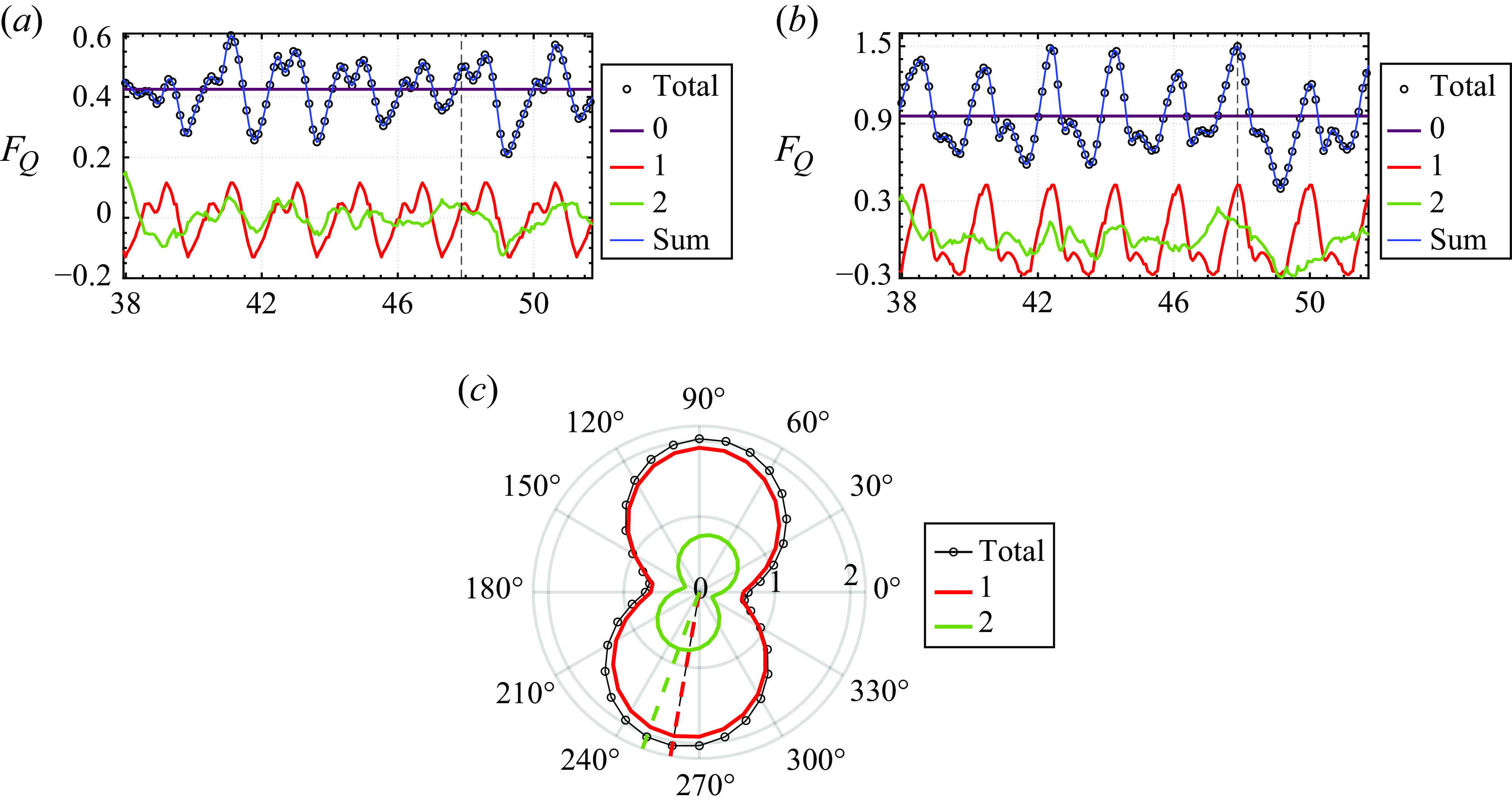
Figure 16. Results from triple decomposition applied directly to the
 $Q$
-field of the aerofoil. Temporal variation of the vortex-induced (a) drag force (
$Q$
-field of the aerofoil. Temporal variation of the vortex-induced (a) drag force (
 $F_Q^{(1)}$
) and (b) lift force (
$F_Q^{(1)}$
) and (b) lift force (
 $F_Q^{(2)}$
) corresponding to the modes of the triple decomposition. The vortex-induced lift force is normalised using the force coefficient (
$F_Q^{(2)}$
) corresponding to the modes of the triple decomposition. The vortex-induced lift force is normalised using the force coefficient (
 $0.5\rho U_\infty ^2 c$
), and the time is normalised using the flow time scale (
$0.5\rho U_\infty ^2 c$
), and the time is normalised using the flow time scale (
 $c/U_\infty$
). (c) The directivity (
$c/U_\infty$
). (c) The directivity (
 $p'_{rms}\times 10^{-5}$
) calculated at distance
$p'_{rms}\times 10^{-5}$
) calculated at distance
 $57c$
, corresponding to Mach number 0.1, with the dashed line showing the directivity of the highest sound intensity.
$57c$
, corresponding to Mach number 0.1, with the dashed line showing the directivity of the highest sound intensity.
The aerodynamic sound is again computed by applying the FAPM to the triple-decomposed
 $Q$
-fields. The directivity patterns for the dipole sounds generated by the fluctuating aerodynamic forces are shown in figure 16(c). The aerodynamic sound is evaluated at distance
$Q$
-fields. The directivity patterns for the dipole sounds generated by the fluctuating aerodynamic forces are shown in figure 16(c). The aerodynamic sound is evaluated at distance
 $57c$
away from the aerofoil, with flow Mach number 0.1. As one can expect, most of the noise produced by the aerofoil comes from the high-amplitude coherent mode (Mode-1), while the noise from the incoherent mode is noticeably weaker. It is interesting to note that the directivity peaks for the two modes are slightly different, as marked in figure 16(c). Indeed, the directivity of the incoherent mode is tilted further away (by approximately
$57c$
away from the aerofoil, with flow Mach number 0.1. As one can expect, most of the noise produced by the aerofoil comes from the high-amplitude coherent mode (Mode-1), while the noise from the incoherent mode is noticeably weaker. It is interesting to note that the directivity peaks for the two modes are slightly different, as marked in figure 16(c). Indeed, the directivity of the incoherent mode is tilted further away (by approximately
 $10^\circ$
) from the vertical axis compared to the coherent mode, and this is directly connected with the decreased lift-to-drag fluctuation ratio of the incoherent mode compared to the coherent mode, as discussed above. Thus modal force partitioning when applied to the
$10^\circ$
) from the vertical axis compared to the coherent mode, and this is directly connected with the decreased lift-to-drag fluctuation ratio of the incoherent mode compared to the coherent mode, as discussed above. Thus modal force partitioning when applied to the
 $Q$
-field results in interpretable insights that are difficult to obtain using other approaches. Furthermore, modal force partitioning provides a novel and useful method to connect the coherent and incoherent modes to distinct characteristics of the aerodynamic force as well as the amplitude and directivity characteristics of the aeroacoustic sound.
$Q$
-field results in interpretable insights that are difficult to obtain using other approaches. Furthermore, modal force partitioning provides a novel and useful method to connect the coherent and incoherent modes to distinct characteristics of the aerodynamic force as well as the amplitude and directivity characteristics of the aeroacoustic sound.
3.3. Revolving wing
In this subsection, we model a single rotor blade with the geometry based on the experimental study of Gururaj et al. (Reference Gururaj, Moaven, Tan, Thurow and Raghav2021). The rotor blade is a rectangular flat plate with aspect ratio 5, and the angle of attack is set to 45
 $^\circ$
. The blade revolves with angular velocity
$^\circ$
. The blade revolves with angular velocity
 $0.25 v_t/R_c$
, where
$0.25 v_t/R_c$
, where
 $v_t$
is the tip velocity, and
$v_t$
is the tip velocity, and
 $R_c$
is the distance from the centre of revolution to the tip of the blade. The blade is modelled as a zero thickness plate, and the simulation is performed in a non-inertial rotating reference frame with Reynolds number 3300 based on the tip velocity (
$R_c$
is the distance from the centre of revolution to the tip of the blade. The blade is modelled as a zero thickness plate, and the simulation is performed in a non-inertial rotating reference frame with Reynolds number 3300 based on the tip velocity (
 $v_t$
) and the radius measured from centre of revolution (
$v_t$
) and the radius measured from centre of revolution (
 $R_c$
). The Reynolds number based on the tip velocity and the chord length is 500. The domain size used for this simulation is
$R_c$
). The Reynolds number based on the tip velocity and the chord length is 500. The domain size used for this simulation is
 $8R_c \times 10R_c \times 10R_c$
. The mesh and the location of the rotor (in red) are shown in figure 17(a), and we point out that a very fine mesh is employed over the region
$8R_c \times 10R_c \times 10R_c$
. The mesh and the location of the rotor (in red) are shown in figure 17(a), and we point out that a very fine mesh is employed over the region
 $5c \times 2.4R_c \times 2.4R_c$
to resolve the vortices generated over the blade and in its wake.
$5c \times 2.4R_c \times 2.4R_c$
to resolve the vortices generated over the blade and in its wake.
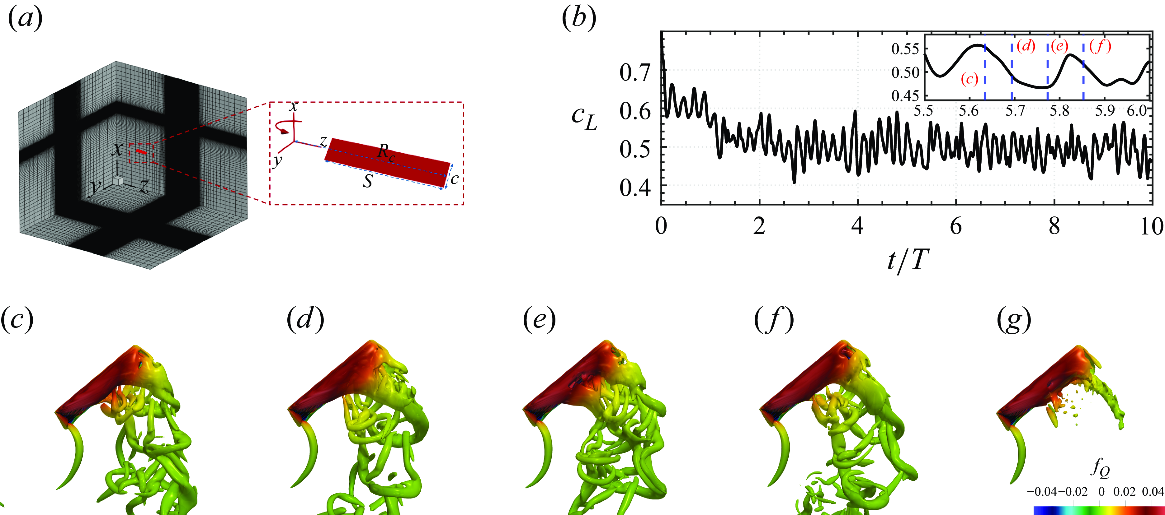
Figure 17. (a) The computational domain and mesh for the rotor simulation, with a zoomed image of the rotor with axis shown at the centre of the revolution. (b) The lift coefficient (normalised using tip velocity and the rotor area) for the rotor, with vertical lines showing the time instances where the flow vortex structures are shown. (c–f) Instantaneous flow fields showing the shedding of the vortices, and (g) the mean flow. The vortices are shown using the
 $Q$
-field and coloured by the vortex-induced lift force.
$Q$
-field and coloured by the vortex-induced lift force.
3.3.1. Flow characteristics and aerodynamic loads
The flow simulation is carried out for 10 revolution cycles, and the time history of the lift coefficient is plotted in figure 17(b). The instantaneous flow fields are visualised by
 $Q$
-fields in figures 17(c–f) at four time instances marked by the vertical dashed blue lines on the lift coefficient profile. In addition, the mean flow obtained from averaging over revolution cycles 5–10 is also shown in figure 17(g). We see a smooth root vortex and LEV that sheds in two locations along the span: one at approximately the 50 % chord (visible in figure 17
d), and one closer to the blade tip (visible in figures 17
c,f) where it merges with the blade-tip vortex. Indeed, figure 17(e) shows both these phenomena occurring at the same time. Careful examination of the plots also indicates the formation and shedding of secondary LEVs. Vortices are also shed from the trailing edge of the blade, and all of these vortices interact in a complex way in the wake region of the blade.
$Q$
-fields in figures 17(c–f) at four time instances marked by the vertical dashed blue lines on the lift coefficient profile. In addition, the mean flow obtained from averaging over revolution cycles 5–10 is also shown in figure 17(g). We see a smooth root vortex and LEV that sheds in two locations along the span: one at approximately the 50 % chord (visible in figure 17
d), and one closer to the blade tip (visible in figures 17
c,f) where it merges with the blade-tip vortex. Indeed, figure 17(e) shows both these phenomena occurring at the same time. Careful examination of the plots also indicates the formation and shedding of secondary LEVs. Vortices are also shed from the trailing edge of the blade, and all of these vortices interact in a complex way in the wake region of the blade.
The
 $Q$
-field associated with the mean flow shown in figure 17(g) shows only vortices near the root and the blade tip as well as the leading edge, but the vortex dynamics and associated aerodynamic loads and aeroacoustic sound are associated with a very complex behaviour, evident in the instantaneous snapshots. Thus the task of determining the flow modes with dominant contributions to the aerodynamic loads and aeroacoustic sound is significantly more complex. Based on our discussion in the previous subsections, we choose to directly decompose the
$Q$
-field associated with the mean flow shown in figure 17(g) shows only vortices near the root and the blade tip as well as the leading edge, but the vortex dynamics and associated aerodynamic loads and aeroacoustic sound are associated with a very complex behaviour, evident in the instantaneous snapshots. Thus the task of determining the flow modes with dominant contributions to the aerodynamic loads and aeroacoustic sound is significantly more complex. Based on our discussion in the previous subsections, we choose to directly decompose the
 $Q$
-field to eliminate the inter-modal interactions.
$Q$
-field to eliminate the inter-modal interactions.
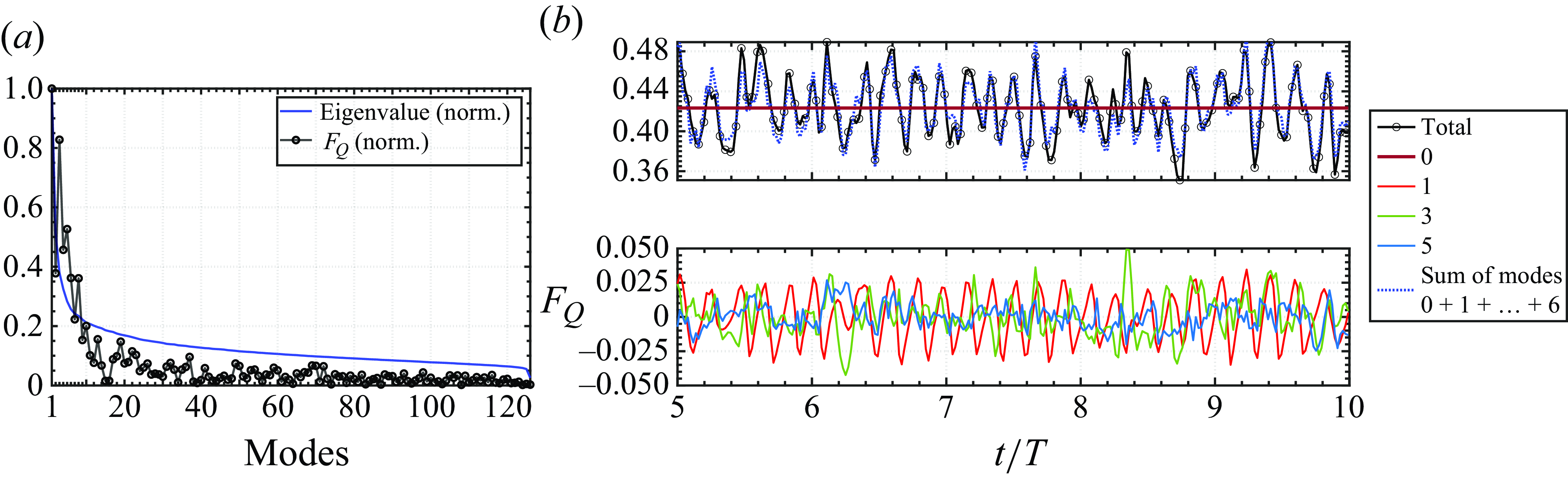
Figure 18. (a) Eigenvalues corresponding to POD modes along with the vortex-induced lift force (
 $F_Q^{(2)}$
) corresponding to each mode. (b) Vortex-induced lift force versus time corresponding to the POD applied on
$F_Q^{(2)}$
) corresponding to each mode. (b) Vortex-induced lift force versus time corresponding to the POD applied on
 $Q$
, showing the dominant modes. The vortex-induced lift force is normalised using tip velocity and the rotor area, while the time is normalised using the time period of each revolution (
$Q$
, showing the dominant modes. The vortex-induced lift force is normalised using tip velocity and the rotor area, while the time is normalised using the time period of each revolution (
 $T$
).
$T$
).
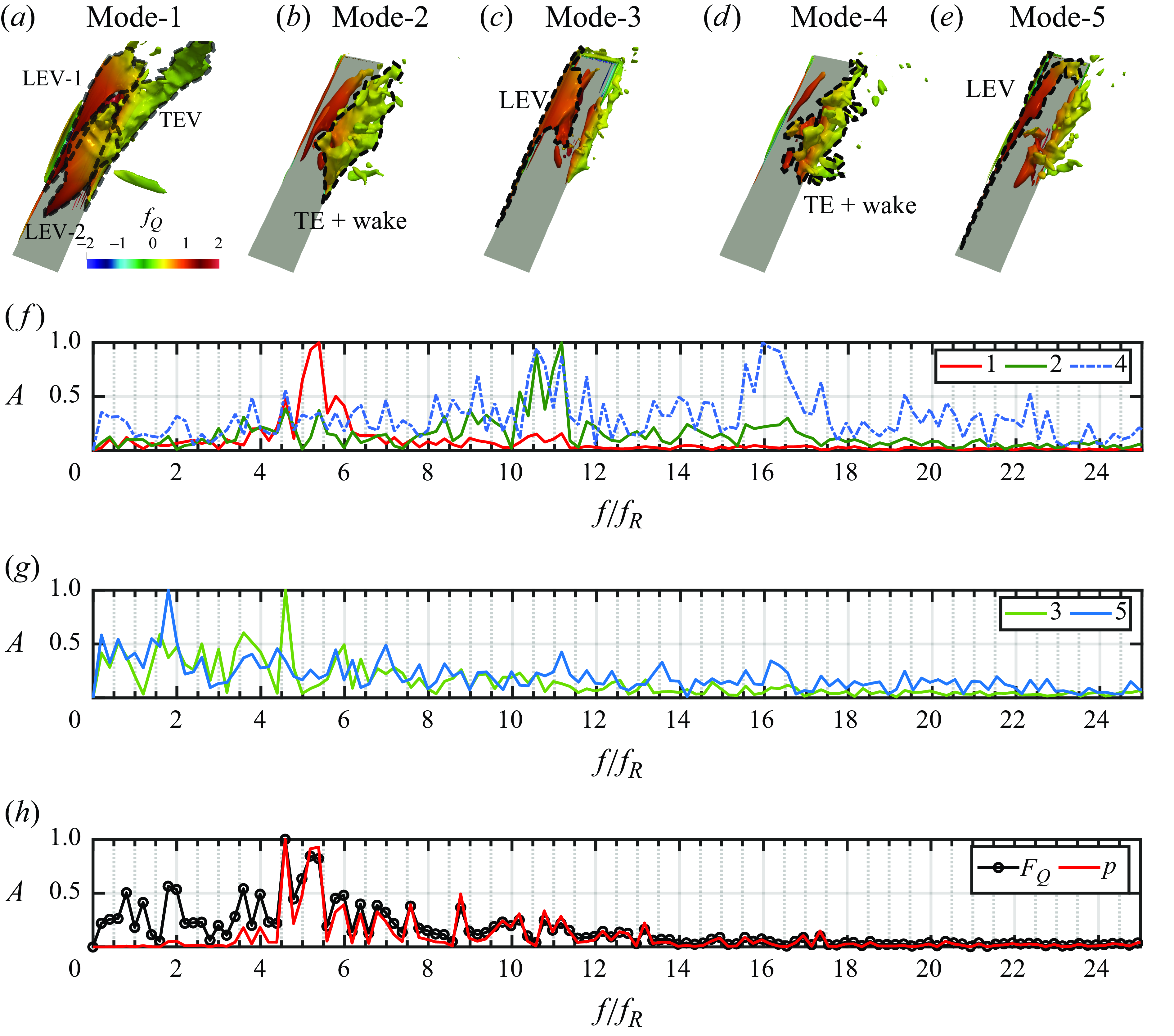
Figure 19. Results for modal force partitioning applied to POD of the
 $Q$
-field. Plots of the scaled spatial eigenvectors (
$Q$
-field. Plots of the scaled spatial eigenvectors (
 $U \Sigma$
) of the rotor showing isosurfaces of the
$U \Sigma$
) of the rotor showing isosurfaces of the
 $Q$
-field coloured by the vortex-induced lift force (
$Q$
-field coloured by the vortex-induced lift force (
 $f_Q^{(2)})$
corresponding to (a) Mode-1, (b) Mode-2, (c) Mode-3, (d) Mode-4 and (e) Mode-5. The frequency spectrum of the temporal eigenvector (
$f_Q^{(2)})$
corresponding to (a) Mode-1, (b) Mode-2, (c) Mode-3, (d) Mode-4 and (e) Mode-5. The frequency spectrum of the temporal eigenvector (
 $V^T$
) of the POD for (f) Mode-1, Mode-2, Mode-4, and (g) Mode-3, Mode-5. (h) The frequency spectrum for the total vortex-induced lift force (
$V^T$
) of the POD for (f) Mode-1, Mode-2, Mode-4, and (g) Mode-3, Mode-5. (h) The frequency spectrum for the total vortex-induced lift force (
 $F_Q^{(2)}$
) and the sound pressure (
$F_Q^{(2)}$
) and the sound pressure (
 $p'$
) at
$p'$
) at
 $200R_c$
, 90
$200R_c$
, 90
 $^\circ$
. The amplitude for each mode is normalised by its respective maximum value to highlight the spectral content of each mode, and the frequency is normalised by the revolution frequency (
$^\circ$
. The amplitude for each mode is normalised by its respective maximum value to highlight the spectral content of each mode, and the frequency is normalised by the revolution frequency (
 $f_R$
).
$f_R$
).
3.3.2. The mFPM applied to POD of the
$Q$
-field

The POD is applied to the
 $Q$
-field of the flow over revolution cycles
$Q$
-field of the flow over revolution cycles
 $t/T=5{-}10$
, with 50 snapshots in each cycle, and the eigenvalues for the modes are shown in figure 18(a); 121 modes are required in this case to reconstruct 98 % of the original
$t/T=5{-}10$
, with 50 snapshots in each cycle, and the eigenvalues for the modes are shown in figure 18(a); 121 modes are required in this case to reconstruct 98 % of the original
 $Q$
-field. The contribution of each mode to the vortex-induced lift force (
$Q$
-field. The contribution of each mode to the vortex-induced lift force (
 $F_Q$
) is also plotted in the figure. Note that since the angle of attack of the blade is
$F_Q$
) is also plotted in the figure. Note that since the angle of attack of the blade is
 $45^\circ$
, the pressure lift is identically equal to the pressure drag for this case. The normalised value of
$45^\circ$
, the pressure lift is identically equal to the pressure drag for this case. The normalised value of
 $F_Q$
shows that the three dominant modes for the aerodynamic lift force are modes 1, 3 and 5. This also suggests that these three modes could possibly be the dominant sources of the aerodynamic loading noise as well, since the dipole loading noise for a rotor is generated by the pressure force fluctuation on the rotor blades. While we expect the POD mode of
$F_Q$
shows that the three dominant modes for the aerodynamic lift force are modes 1, 3 and 5. This also suggests that these three modes could possibly be the dominant sources of the aerodynamic loading noise as well, since the dipole loading noise for a rotor is generated by the pressure force fluctuation on the rotor blades. While we expect the POD mode of
 $Q$
to be arranged with decreasing ‘energy’ content, the net force depends on the product of
$Q$
to be arranged with decreasing ‘energy’ content, the net force depends on the product of
 $Q$
and the influence field (
$Q$
and the influence field (
 $\phi$
). With
$\phi$
). With
 $\phi$
decreasing rapidly away from the surface of the rotor, the modes containing larger vortical structures near the rotor will contribute more towards the aerodynamic force, hence we do not see a monotonic reduction in the net force generated by these modes.
$\phi$
decreasing rapidly away from the surface of the rotor, the modes containing larger vortical structures near the rotor will contribute more towards the aerodynamic force, hence we do not see a monotonic reduction in the net force generated by these modes.
We find that the cumulative value of the vortex-induced lift force converges very rapidly to the value of the total vortex-induced lift force. Furthermore, the first six modes capture 91.3 % of the total variance in the lift. The corresponding time histories of the vortex-induced lift forces are shown in figure 18(b), and we see most of the large-amplitude fluctuations being captured by the dominant modes (1, 3 and 5). We note that while Mode-1 captures the most periodic component of the force fluctuation, the intermittent, lower-frequency force fluctuations are represented by Mode-3. Mode-5, on the other hand, generates smaller-scale but highly stochastic variations in the force. The sum of the first six modes (1–6) and the mean is a good approximation of the total force, as shown in figure 18(b), although we see in figure 18(a) that several higher modes contribute to the total vortex-induced lift force. Thus even though a large number of modes generate contributions to the
 $Q$
-field and the vortex-induced lift force, just a few of the first few modes of the
$Q$
-field and the vortex-induced lift force, just a few of the first few modes of the
 $Q$
-field recover most of the aerodynamic force. Thus this modal force partitioning approach provides a highly compact representation of the force-generating modes.
$Q$
-field recover most of the aerodynamic force. Thus this modal force partitioning approach provides a highly compact representation of the force-generating modes.
We now examine the spatial and temporal topology of the dominant force-generating modes by separating the spatial structure and temporal variation of these modes. The spatial structure of these dominant POD modes (1–5) is visualised via the spatial eigenvector times the corresponding eigenvalues (
 $U\Sigma$
) in figures 19(a–e). While these modes have complex topologies, some useful observations can be made. First, Mode-1 is dominated by at least three distinct structures: an LEV that separates near the mid-span (denoted as ‘LEV-1’ in the figure), an LEV that extends from the mid-span to the blade-tip (‘LEV-2’), and a trailing-edge vortex (‘TEV’) that also extends from the mid-span to the blade-tip. Mode-3 and Mode-5 also clearly show leading-edge vortices (‘LEV’ in the figure), whereas Mode-2 and Mode-4 show structures associated with the trailing edge and near-wake vortices (‘TE + wake’ in the figure). These topologies provide some sense of the vortical phenomenon that is represented by these modes, and also provide a phenomenological connection to the force generation. For instance, since the LEV is a major contributor to the aerodynamic lift, it is not surprising that Mode-1, Mode-3 and Mode-5 provide most of the vortex-induced lift force (figure 18
a).
$U\Sigma$
) in figures 19(a–e). While these modes have complex topologies, some useful observations can be made. First, Mode-1 is dominated by at least three distinct structures: an LEV that separates near the mid-span (denoted as ‘LEV-1’ in the figure), an LEV that extends from the mid-span to the blade-tip (‘LEV-2’), and a trailing-edge vortex (‘TEV’) that also extends from the mid-span to the blade-tip. Mode-3 and Mode-5 also clearly show leading-edge vortices (‘LEV’ in the figure), whereas Mode-2 and Mode-4 show structures associated with the trailing edge and near-wake vortices (‘TE + wake’ in the figure). These topologies provide some sense of the vortical phenomenon that is represented by these modes, and also provide a phenomenological connection to the force generation. For instance, since the LEV is a major contributor to the aerodynamic lift, it is not surprising that Mode-1, Mode-3 and Mode-5 provide most of the vortex-induced lift force (figure 18
a).
Beyond the spatial structure, the temporal content of these modes is an important differentiator of these modes as well, and in figures 19(f) and 19(g), we show the frequency spectrum of the temporal eigenvectors contained within
 $V$
corresponding to these first five modes, and several observations can be made from these plots. First, Mode-1 is dominated by a fairly narrow band of frequencies, centred around 5.2 (designated here by
$V$
corresponding to these first five modes, and several observations can be made from these plots. First, Mode-1 is dominated by a fairly narrow band of frequencies, centred around 5.2 (designated here by
 $f_0$
). Mode-2 primarily contains
$f_0$
). Mode-2 primarily contains
 $2f_0$
, while Mode-4 is characterised by both
$2f_0$
, while Mode-4 is characterised by both
 $2f_0$
and
$2f_0$
and
 $3f_0$
. Thus these three modes are likely connected with the periodic shedding of multiple vortices from the leading edge and trailing edge of the blade. Mode-3 has a clearly dominant frequency at 4.58, and this combined with the spatial structure suggests that this is the shedding of yet another LEV from near the 75 % span of the blade. Finally, Mode-5 corresponds to a low frequency (1.79) mode, which could be a subharmonic mode of one of the other dominant modes. Figure 19(h) shows the spectrum of the total lift force as well as that of the sound pressure at
$3f_0$
. Thus these three modes are likely connected with the periodic shedding of multiple vortices from the leading edge and trailing edge of the blade. Mode-3 has a clearly dominant frequency at 4.58, and this combined with the spatial structure suggests that this is the shedding of yet another LEV from near the 75 % span of the blade. Finally, Mode-5 corresponds to a low frequency (1.79) mode, which could be a subharmonic mode of one of the other dominant modes. Figure 19(h) shows the spectrum of the total lift force as well as that of the sound pressure at
 $200R_c$
, 90
$200R_c$
, 90
 $^\circ$
, and we note that the dominant peaks in both these quantities are in the vicinity of frequency 5.0 and clearly connected with Mode-1 and Mode-3. The lift force and sound pressure are in very good agreement for the higher frequencies. For the lower frequencies, the sound pressure is of very small amplitude, and this mismatch to the lift is due to the fact that the far-field sound originates from the time derivative of the force, thus the amplitude in the low-frequency range is reduced by its multiplication with the frequency.
$^\circ$
, and we note that the dominant peaks in both these quantities are in the vicinity of frequency 5.0 and clearly connected with Mode-1 and Mode-3. The lift force and sound pressure are in very good agreement for the higher frequencies. For the lower frequencies, the sound pressure is of very small amplitude, and this mismatch to the lift is due to the fact that the far-field sound originates from the time derivative of the force, thus the amplitude in the low-frequency range is reduced by its multiplication with the frequency.
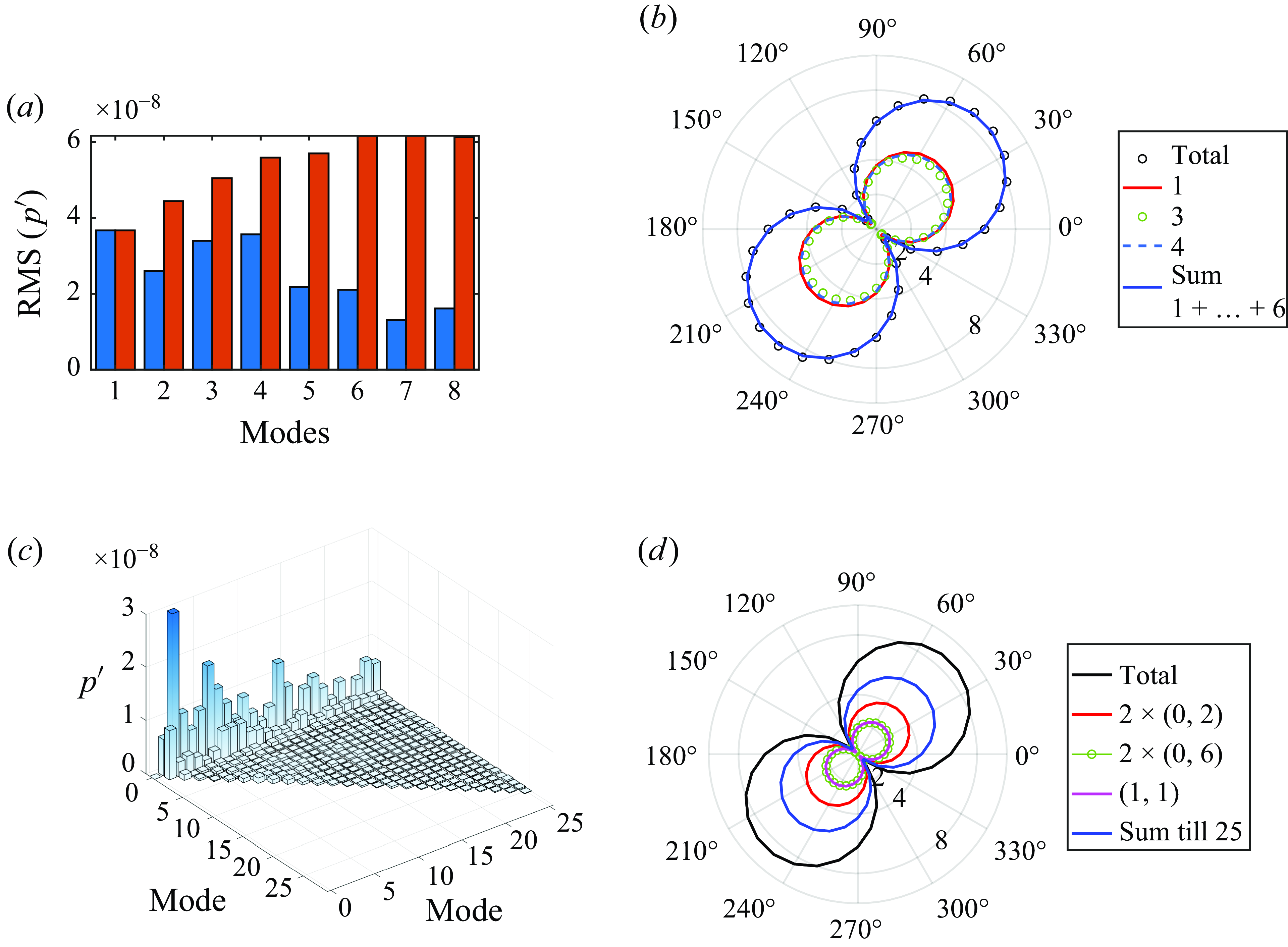
Figure 20. Results from modal force and acoustic partitioning applied to the POD of the
 $Q$
-field for the rotor blade: (a) the RMS value of the sound pressure for the first eight modes in blue, and their cumulative values in red; (b) the directivity (
$Q$
-field for the rotor blade: (a) the RMS value of the sound pressure for the first eight modes in blue, and their cumulative values in red; (b) the directivity (
 $p'_{rms}\times 10^{-8}$
) for some dominant modes. Results from modal force and acoustic partitioning applied to the POD of the velocity field for the rotor blade: (c) the RMS of sound pressure level for first 25 modal interactions; (d) the directivity (
$p'_{rms}\times 10^{-8}$
) for some dominant modes. Results from modal force and acoustic partitioning applied to the POD of the velocity field for the rotor blade: (c) the RMS of sound pressure level for first 25 modal interactions; (d) the directivity (
 $p'_{rms}\times 10^{-8}$
) corresponding to some dominant modes and modal interactions. The sound in all of these plots is measured at adistance
$p'_{rms}\times 10^{-8}$
) corresponding to some dominant modes and modal interactions. The sound in all of these plots is measured at adistance
 $200R_c$
away, and corresponds to the tip-velocity-based Mach number 0.25. The RMS values of the sound pressure level are recorded at a 90
$200R_c$
away, and corresponds to the tip-velocity-based Mach number 0.25. The RMS values of the sound pressure level are recorded at a 90
 $^\circ$
angular orientation relative to the centre of the rotor.
$^\circ$
angular orientation relative to the centre of the rotor.
Finally, the aeroacoustic sound generated by the revolving wing is calculated at a distance
 $200R_c$
away from the revolution centre, and tip-velocity-based Mach number 0.25. The RMS value of the sound pressure for each mode, recorded at angular location 90
$200R_c$
away from the revolution centre, and tip-velocity-based Mach number 0.25. The RMS value of the sound pressure for each mode, recorded at angular location 90
 $^\circ$
(this corresponds to a point vertically above the revolution centre), is shown in figure 20(a). We note that similar to the vortex-induced lift force results, the sound pressure generated by these modes could easily be captured by a few dominant modes. Specifically, Mode-1, Mode-3 and Mode-4 are found to be the top three dominant modes for the aeroacoustic noise. Figure 20(b) shows that by solely considering the first six modes, we almost fully match the sound directivity pattern for the rotor blade.
$^\circ$
(this corresponds to a point vertically above the revolution centre), is shown in figure 20(a). We note that similar to the vortex-induced lift force results, the sound pressure generated by these modes could easily be captured by a few dominant modes. Specifically, Mode-1, Mode-3 and Mode-4 are found to be the top three dominant modes for the aeroacoustic noise. Figure 20(b) shows that by solely considering the first six modes, we almost fully match the sound directivity pattern for the rotor blade.
For comparison, figures 20(c) and 20(d) show results from modal force and acoustic partitioning applied to the POD of the velocity field for the rotor blade. The contributions of intra-modal and inter-modal interactions to the sound pressure are shown in figure 20(c), and we note that inter-modal interactions of Mode-0, Mode-1 and Mode-2 with all the other modes (we show only up to Mode-25) make significant contributions to the sound field. Indeed, the two largest contributions are from the (0,2) and (0,6) modes. We also note from figure 20(d) that even the addition of all the intra-modal and inter-modal contributions from Mode-1 to Mode-25 does not provide a good estimate of the total sound directivity. Chiu et al. (Reference Chiu, Tseng, Chang and Chou2023) employed the ‘force representation theory’ wherein, instead of
 $Q$
, the force density is based on the Lamb vector as
$Q$
, the force density is based on the Lamb vector as
 $ ( \boldsymbol{u}\times \boldsymbol{\omega } ) \boldsymbol{\cdot} \boldsymbol{\nabla} \phi$
. They applied their method to an SPOD of the velocity flow field, and due to the nonlinearity of the Lamb vector, they also encountered inter-modal interaction between the SPOD modes, which complicated the interpretability of their results. Based on our experience, a direct SPOD of the Lamb vector would alleviate this issue for their method as well.
$ ( \boldsymbol{u}\times \boldsymbol{\omega } ) \boldsymbol{\cdot} \boldsymbol{\nabla} \phi$
. They applied their method to an SPOD of the velocity flow field, and due to the nonlinearity of the Lamb vector, they also encountered inter-modal interaction between the SPOD modes, which complicated the interpretability of their results. Based on our experience, a direct SPOD of the Lamb vector would alleviate this issue for their method as well.
4. Conclusions
In order to identify the flow structures (or modes) that contribute significantly to aerodynamic force and aeroacoustic sound generation in complex flows, we propose a modal force and acoustic decomposition method by combining the previously developed force and acoustic partitioning method (FAPM) (Zhang et al. Reference Zhang, Hedrick and Mittal2015; Menon & Mittal Reference Menon and Mittal2021a
; Seo et al. Reference Seo, Menon and Mittal2022) with the modal decomposition of flows. The modal FAPM is applied first to a canonical case of flow past a 2-D circular cylinder at
 $Re=300$
and flow past an NACA 0015 aerofoil at higher Reynolds number 2500 to examine the implications of applying FAPM to modes obtained from various decomposition techniques, such as Reynolds decomposition, triple decomposition and POD. Because the aerodynamic force is determined by the
$Re=300$
and flow past an NACA 0015 aerofoil at higher Reynolds number 2500 to examine the implications of applying FAPM to modes obtained from various decomposition techniques, such as Reynolds decomposition, triple decomposition and POD. Because the aerodynamic force is determined by the
 $Q$
-field, which is a nonlinear observable of the flow, modal decomposition of the velocity field leads to a situation where nonlinear interactions between the decomposed modes become important in the determination of the aerodynamic loads and aeroacoustic sound. These inter-modal interactions make it difficult to interpret the contributions of individual modes to aerodynamic loading and aeroacoustic sound.
$Q$
-field, which is a nonlinear observable of the flow, modal decomposition of the velocity field leads to a situation where nonlinear interactions between the decomposed modes become important in the determination of the aerodynamic loads and aeroacoustic sound. These inter-modal interactions make it difficult to interpret the contributions of individual modes to aerodynamic loading and aeroacoustic sound.
Based on this observation, we propose the direct modal decomposition of the
 $Q$
-field. This approach eliminates inter-modal interactions from modal aerodynamic loads and aeroacoustic sound associated with the modes. The application of this approach to the circular cylinder flow shows that the modes and forces obtained from this decomposition exhibit certain symmetries that make it easier to interpret the significance of different modes. When triple decomposition is applied directly to the
$Q$
-field. This approach eliminates inter-modal interactions from modal aerodynamic loads and aeroacoustic sound associated with the modes. The application of this approach to the circular cylinder flow shows that the modes and forces obtained from this decomposition exhibit certain symmetries that make it easier to interpret the significance of different modes. When triple decomposition is applied directly to the
 $Q$
-field for the aerofoil, we find, for instance, that the sound induced by the incoherent component has a larger contribution from the induced drag than for the coherent contribution. This has interpretable implications for the directivity of sound for these two modes. We also use modal acoustic partitioning to compute the distinct sound spectra for the coherent and incoherent modes. To our knowledge, this type of partitioning of sound sources has not been demonstrated before.
$Q$
-field for the aerofoil, we find, for instance, that the sound induced by the incoherent component has a larger contribution from the induced drag than for the coherent contribution. This has interpretable implications for the directivity of sound for these two modes. We also use modal acoustic partitioning to compute the distinct sound spectra for the coherent and incoherent modes. To our knowledge, this type of partitioning of sound sources has not been demonstrated before.
The final application of the modal force and acoustic partitioning is to a relatively complex case of a revolving rectangular wing at tip Reynolds number 3300. This configuration generates a complex 3-D flow that requires 119 POD velocity modes to reconstruct 98 % of the velocity field. Modal force and acoustic partitioning applied to the POD modes obtained from the velocity field exhibit very significant contributions from inter-modal interactions. In contrast, POD of the
 $Q$
-field eliminates the inter-modal interactions, and indicates that three dominant modes modes (Mode-1, Mode-3 and Mode-4) contribute 69.4 % of the total aeroacoustic sound (calculated based on the acoustic intensity), and the sum of the first six POD modes recovers nearly all the aeroacoustic sound contributions. Thus POD applied to the
$Q$
-field eliminates the inter-modal interactions, and indicates that three dominant modes modes (Mode-1, Mode-3 and Mode-4) contribute 69.4 % of the total aeroacoustic sound (calculated based on the acoustic intensity), and the sum of the first six POD modes recovers nearly all the aeroacoustic sound contributions. Thus POD applied to the
 $Q$
-field demonstrates that even for this relatively complex 3-D flow, the aerodynamic loads and aeroacoustic sound can be represented by a set of modes that are significantly more compact than those required for the flow itself.
$Q$
-field demonstrates that even for this relatively complex 3-D flow, the aerodynamic loads and aeroacoustic sound can be represented by a set of modes that are significantly more compact than those required for the flow itself.
Modal decompositions are considered primarily tools for examining the kinematics of the flow and for developing low-dimensional representations of the flow field. However, the contributions of these modes to the aerodynamic loads, which are quite often key quantities of interest, are not usually considered because there has not been a systematic way to compute the aerodynamic loads for the decomposed flow modes. The modal force partitioning method (mFPM) proposed here provides this capability. The direct modal decomposition of
 $Q$
enables us to determine the modes that make the dominant contribution to the aerodynamic loads. This also suggests that
$Q$
enables us to determine the modes that make the dominant contribution to the aerodynamic loads. This also suggests that
 $Q$
, which has mostly been used for identification of vortices in flows, is a nonlinear observable with exceptional importance in the analysis of aerodynamic loads. In addition to the applications for determining the mechanisms for the generation of aerodynamic loads and aeroacoustic sound explored here, it is expected that modal force partitioning will find use in several other arenas, including flow-induced vibration/flutter and flow control.
$Q$
, which has mostly been used for identification of vortices in flows, is a nonlinear observable with exceptional importance in the analysis of aerodynamic loads. In addition to the applications for determining the mechanisms for the generation of aerodynamic loads and aeroacoustic sound explored here, it is expected that modal force partitioning will find use in several other arenas, including flow-induced vibration/flutter and flow control.
In closing, we note that while the current paper had focused on Reynolds decomposition, triple decomposition and POD, modal force partitioning can in principle be applied equally well to other modal decomposition techniques. In particular, new methods for dimensionality reduction based on machine-learning techniques and neural networks are being developed (Fukami & Taira Reference Fukami and Taira2023; Solera-Rico et al. Reference Solera-Rico, Vila, Gómez-López, Wang, Almashjary, Dawson and Vinuesa2024), and it would be interesting to apply the FPM in conjunction with these techniques. Finally, while the current study applies mFPM to results from direct numerical simulations, FPM and mFPM could also be applied to data from large-eddy simulations where one would have to account for the contributions of the subgrid-scale stress term to the surface pressure force. These are useful directions to pursue in a future study.
Funding
The authors acknowledge support from the Army Research Office (Cooperative Agreement no. W911NF2120087) for this work. Computational resources for this work were provided by the Advanced Research Computing at Hopkins (ARCH) core facility (rockfish.jhu.edu) and high-performance computer time and resources from the DoD High Performance Computing Modernisation Program.
Declaration of interests
The authors report no conflict of interest.
Appendix A. Derivation of the FPM
The derivation of the FPM can be found in previous papers (Zhang et al. Reference Zhang, Hedrick and Mittal2015; Menon & Mittal, Reference Menon and Mittal2021c
; Menon, Kumar & Mittal Reference Menon, Kumar and Mittal2022), but it is included here for the sake of completeness. The gradient of the field of influence
 $\phi$
(see (2.1)) is projected onto the Navier–Stokes equation (2.3), which results in the following equation:
$\phi$
(see (2.1)) is projected onto the Navier–Stokes equation (2.3), which results in the following equation:
 \begin{equation} \int _{V_f} \rho \left [ \frac {\partial \boldsymbol{u}}{\partial t} + \boldsymbol{u} \boldsymbol{\cdot} \boldsymbol{\nabla} \boldsymbol{u} \right ]\boldsymbol{\cdot} \boldsymbol{\nabla} \phi ^{(i)}\, {\rm d}V= \int _{V_f} \left [ -{\boldsymbol{\nabla}} P +\mu\, \boldsymbol{\nabla} ^2 \boldsymbol{u} \right ] \boldsymbol{\cdot} {\boldsymbol{\nabla}} \phi ^{(i)}\, {\rm d}V . \end{equation}
Rearranging the terms, we get
 \begin{equation} -\int _{V_f}{\boldsymbol{\nabla}} P \boldsymbol{\cdot} {\boldsymbol{\nabla}} \phi ^{(i)}\, {\rm d}V= \int _{V_f} \left [\rho \frac {\partial \boldsymbol{u}}{\partial t}\boldsymbol{\cdot} \boldsymbol{\nabla} \phi ^{(i)} + \rho (\boldsymbol{u} \boldsymbol{\cdot} \boldsymbol{\nabla} \boldsymbol{u})\boldsymbol{\cdot} \boldsymbol{\nabla} \phi ^{(i)} - \mu\, \boldsymbol{\nabla} ^2 \boldsymbol{u} \boldsymbol{\cdot} \boldsymbol{\nabla} \phi ^{(i)} \right ] {\rm d}V . \end{equation}
Since
 $\boldsymbol{\nabla} \boldsymbol{\cdot} (P\, \boldsymbol{\nabla} \phi ^{(i)})=\boldsymbol{\nabla} P\boldsymbol{\cdot} \boldsymbol{\nabla} \phi ^{(i)} + P\boldsymbol{\cdot} \boldsymbol{\nabla} ^2 \phi ^{(i)}$
, rearranging these terms, we see that
$\boldsymbol{\nabla} \boldsymbol{\cdot} (P\, \boldsymbol{\nabla} \phi ^{(i)})=\boldsymbol{\nabla} P\boldsymbol{\cdot} \boldsymbol{\nabla} \phi ^{(i)} + P\boldsymbol{\cdot} \boldsymbol{\nabla} ^2 \phi ^{(i)}$
, rearranging these terms, we see that
 $\boldsymbol{\nabla} P\boldsymbol{\cdot} \boldsymbol{\nabla} \phi ^{(i)}=\boldsymbol{\nabla} \boldsymbol{\cdot} (P\, \boldsymbol{\nabla} \phi ^{(i)})-P\boldsymbol{\cdot} \boldsymbol{\nabla} ^2 \phi ^{(i)}$
. Thus the term on the left-hand side of (A2) can be rewritten as
$\boldsymbol{\nabla} P\boldsymbol{\cdot} \boldsymbol{\nabla} \phi ^{(i)}=\boldsymbol{\nabla} \boldsymbol{\cdot} (P\, \boldsymbol{\nabla} \phi ^{(i)})-P\boldsymbol{\cdot} \boldsymbol{\nabla} ^2 \phi ^{(i)}$
. Thus the term on the left-hand side of (A2) can be rewritten as
 \begin{equation} -\int _{V_f}{\boldsymbol{\nabla}} P \boldsymbol{\cdot} {\boldsymbol{\nabla}} \phi ^{(i)}\, {\rm d}V= -\int _{V_f}\boldsymbol{\nabla} \boldsymbol{\cdot} (P\, \boldsymbol{\nabla} \phi ^{(i)})\,{\rm d}V + \int _{V_f}P\boldsymbol{\cdot} \boldsymbol{\nabla} ^2 \phi ^{(i)}\, {\rm d}V . \end{equation}
Here, the last term is zero due to (2.1), and using the Gauss divergence theorem,
 $-\int _{V_f}\boldsymbol{\nabla} \boldsymbol{\cdot} (P\, \boldsymbol{\nabla} \phi ^{(i)})\,{\rm d}V= -\int _{B+\Sigma } P\, \boldsymbol{n}\boldsymbol{\cdot} \boldsymbol{\nabla} \phi ^{(i)}\,{\rm d}S$
, which can be further simplified using (2.2) to get
$-\int _{V_f}\boldsymbol{\nabla} \boldsymbol{\cdot} (P\, \boldsymbol{\nabla} \phi ^{(i)})\,{\rm d}V= -\int _{B+\Sigma } P\, \boldsymbol{n}\boldsymbol{\cdot} \boldsymbol{\nabla} \phi ^{(i)}\,{\rm d}S$
, which can be further simplified using (2.2) to get
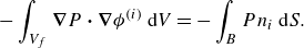 \begin{equation} -\int _{V_f}{\boldsymbol{\nabla}} P \boldsymbol{\cdot} {\boldsymbol{\nabla}} \phi ^{(i)}\, {\rm d}V= -\int _{B} P n_i\, {\rm d}S . \end{equation}
We note that
 $\boldsymbol{\nabla} \boldsymbol{\cdot} ({\partial \boldsymbol{u}}/{\partial t}) \phi =0$
due to the continuity equation, therefore
$\boldsymbol{\nabla} \boldsymbol{\cdot} ({\partial \boldsymbol{u}}/{\partial t}) \phi =0$
due to the continuity equation, therefore
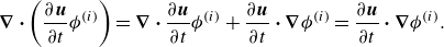 \begin{equation} \boldsymbol{\nabla} \boldsymbol{\cdot} \left(\frac {\partial \boldsymbol{u}}{\partial t} \phi ^{(i)} \right) = \boldsymbol{\nabla} \boldsymbol{\cdot} \frac {\partial \boldsymbol{u}}{\partial t}\phi ^{(i)} + \frac {\partial \boldsymbol{u}}{\partial t} \boldsymbol{\cdot} \boldsymbol{\nabla} \phi ^{(i)} =\frac {\partial \boldsymbol{u}}{\partial t} \boldsymbol{\cdot} \boldsymbol{\nabla} \phi ^{(i)} . \end{equation}
The first term on the right-hand side of (A2) can then be rewritten as
 \begin{equation} \int _{V_f} \rho \frac {\partial \boldsymbol{u}}{\partial t}\boldsymbol{\cdot} \boldsymbol{\nabla} \phi ^{(i)}\, {\rm d}V = \int _{V_f} \rho\, \boldsymbol{\nabla} \boldsymbol{\cdot} \left(\frac {\partial \boldsymbol{u}}{\partial t} \phi ^{(i)} \right) {\rm d}V= \int _{B+\Sigma } \rho\, \boldsymbol{n} \boldsymbol{\cdot} \left(\frac {\partial \boldsymbol{u}}{\partial t} \phi ^{(i)} \right) {\rm d}S . \end{equation}
Similarly,
 \begin{equation} \boldsymbol{\nabla} \boldsymbol{\cdot} ((\boldsymbol{u}\boldsymbol{\cdot} \boldsymbol{\nabla} \boldsymbol{u}) \phi ^{(i)}) = \boldsymbol{\nabla} \boldsymbol{\cdot} (\boldsymbol{u}\boldsymbol{\cdot} \boldsymbol{\nabla} \boldsymbol{u})\phi ^{(i)} + (\boldsymbol{u}\boldsymbol{\cdot} \boldsymbol{\nabla} \boldsymbol{u})\boldsymbol{\cdot} \boldsymbol{\nabla} \phi ^{(i)} , \end{equation}
hence the second right-hand-side term of (A2) can be modified as
 \begin{equation} \int _{V_f} \rho (\boldsymbol{u} \boldsymbol{\cdot} \boldsymbol{\nabla} \boldsymbol{u})\boldsymbol{\cdot} \boldsymbol{\nabla} \phi ^{(i)}\, {\rm d}V=\int _{V_f} \rho\, \boldsymbol{\nabla} \boldsymbol{\cdot} (\boldsymbol{u}\boldsymbol{\cdot} \boldsymbol{\nabla} \boldsymbol{u}\,\phi ^{(i)})\, {\rm d}V-\int _{V_f} \rho\, \boldsymbol{\nabla} \boldsymbol{\cdot} (\boldsymbol{u}\boldsymbol{\cdot} \boldsymbol{\nabla} \boldsymbol{u})\phi ^{(i)}\, {\rm d}V . \end{equation}
The first right-hand-side term in the above equation can again be converted to a surface integral, thus we can write
 $\int _{V_f} \boldsymbol{\nabla} \boldsymbol{\cdot} (\boldsymbol{u}\boldsymbol{\cdot} \boldsymbol{\nabla} \boldsymbol{u}\phi ^{(i)})\, {\rm d}V=\int _{B+\Sigma } \boldsymbol{n} \boldsymbol{\cdot} (\boldsymbol{u}\boldsymbol{\cdot} \boldsymbol{\nabla} \boldsymbol{u}\,\phi ^{(i)})\, {\rm d}S$
. To simplify the second right-hand-side term in the above equation, we use (2.6) and write
$\int _{V_f} \boldsymbol{\nabla} \boldsymbol{\cdot} (\boldsymbol{u}\boldsymbol{\cdot} \boldsymbol{\nabla} \boldsymbol{u}\phi ^{(i)})\, {\rm d}V=\int _{B+\Sigma } \boldsymbol{n} \boldsymbol{\cdot} (\boldsymbol{u}\boldsymbol{\cdot} \boldsymbol{\nabla} \boldsymbol{u}\,\phi ^{(i)})\, {\rm d}S$
. To simplify the second right-hand-side term in the above equation, we use (2.6) and write
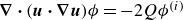 $ \boldsymbol{\nabla} \boldsymbol{\cdot} (\boldsymbol{u}\boldsymbol{\cdot} \boldsymbol{\nabla} \boldsymbol{u})\phi = -2Q\phi ^{(i)}$
. Thus
$ \boldsymbol{\nabla} \boldsymbol{\cdot} (\boldsymbol{u}\boldsymbol{\cdot} \boldsymbol{\nabla} \boldsymbol{u})\phi = -2Q\phi ^{(i)}$
. Thus
 \begin{equation} \int _{V_f} \rho (\boldsymbol{u} \boldsymbol{\cdot} \boldsymbol{\nabla} \boldsymbol{u})\boldsymbol{\cdot} \boldsymbol{\nabla} \phi ^{(i)}\, {\rm d}V=\int _{B+\Sigma } \rho\, \boldsymbol{n} \boldsymbol{\cdot} (\boldsymbol{u}\boldsymbol{\cdot} \boldsymbol{\nabla} \boldsymbol{u}\,\phi ^{(i)})\, {\rm d}S+\int _{V_f} 2\rho Q\phi ^{(i)}\, {\rm d}V . \end{equation}
Equations (A6) and (A9) can be combined to give
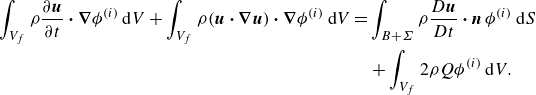 \begin{align} \int _{V_f} \rho \frac {\partial \boldsymbol{u}}{\partial t}\boldsymbol{\cdot} \boldsymbol{\nabla} \phi ^{(i)}\, {\rm d}V + \int _{V_f} \rho (\boldsymbol{u} \boldsymbol{\cdot} \boldsymbol{\nabla} \boldsymbol{u})\boldsymbol{\cdot} \boldsymbol{\nabla} \phi ^{(i)}\, {\rm d}V &= \int _{B+\Sigma } \rho \frac {D\boldsymbol{u}}{Dt} \boldsymbol{\cdot} \boldsymbol{n}\, \phi ^{(i)}\, {\rm d}S\nonumber \\&\quad +\int _{V_f} 2\rho Q\phi ^{(i)} \,{\rm d}V. \end{align}
Next, we consider the last term of (A2), and note that
 $\boldsymbol{\nabla} \boldsymbol{\cdot} (\boldsymbol{\nabla} ^2 \boldsymbol{u}\, \phi ^{(i)})= \boldsymbol{\nabla} \boldsymbol{\cdot} (\boldsymbol{\nabla} ^2 \boldsymbol{u})\phi ^{(i)} + \boldsymbol{\nabla} ^2 \boldsymbol{u} \boldsymbol{\cdot} \boldsymbol{\nabla} \phi ^{(i)}$
. Since
$\boldsymbol{\nabla} \boldsymbol{\cdot} (\boldsymbol{\nabla} ^2 \boldsymbol{u}\, \phi ^{(i)})= \boldsymbol{\nabla} \boldsymbol{\cdot} (\boldsymbol{\nabla} ^2 \boldsymbol{u})\phi ^{(i)} + \boldsymbol{\nabla} ^2 \boldsymbol{u} \boldsymbol{\cdot} \boldsymbol{\nabla} \phi ^{(i)}$
. Since
 $\boldsymbol{\nabla} \boldsymbol{\cdot} (\boldsymbol{\nabla} ^2 \boldsymbol{u})\phi ^{(i)}= (\boldsymbol{\nabla} ^2 \boldsymbol{\nabla} \boldsymbol{\cdot} \boldsymbol{u})\phi ^{(i)}=0$
due to the continuity equation, we can write
$\boldsymbol{\nabla} \boldsymbol{\cdot} (\boldsymbol{\nabla} ^2 \boldsymbol{u})\phi ^{(i)}= (\boldsymbol{\nabla} ^2 \boldsymbol{\nabla} \boldsymbol{\cdot} \boldsymbol{u})\phi ^{(i)}=0$
due to the continuity equation, we can write
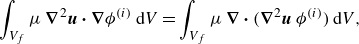 \begin{equation} \int _{V_f}\mu\, \boldsymbol{\nabla} ^2 \boldsymbol{u} \boldsymbol{\cdot} \boldsymbol{\nabla} \phi ^{(i)}\, {\rm d}V= \int _{V_f} \mu\, \boldsymbol{\nabla} \boldsymbol{\cdot} (\boldsymbol{\nabla} ^2 \boldsymbol{u}\, \phi ^{(i)}) \,{\rm d}V , \end{equation}
which is further simplified using the Gauss divergence theorem to give the surface integral as
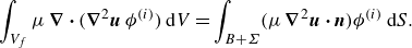 \begin{equation} \int _{V_f} \mu\, \boldsymbol{\nabla} \boldsymbol{\cdot} (\boldsymbol{\nabla} ^2 \boldsymbol{u}\, \phi ^{(i)})\, {\rm d}V = \int _{B+\Sigma } (\mu\, \boldsymbol{\nabla} ^2 \boldsymbol{u}\boldsymbol{\cdot} \boldsymbol{n}) \phi ^{(i)}\, {\rm d}S. \end{equation}
Appendix B. Grid convergence
The grid convergence for the circular cylinder is shown in figure 21(a), with the coarse and fine meshes corresponding to 580 000 and 990 000 total grid points, respectively. The time series for the fine mesh lift coefficient is shifted backwards to match the phase of the time series on the coarse mesh, and the percentage difference between the RMS values of the lift coefficient is 1.34 %. The case with fine mesh is used for all the circular cylinder results presented in this paper.
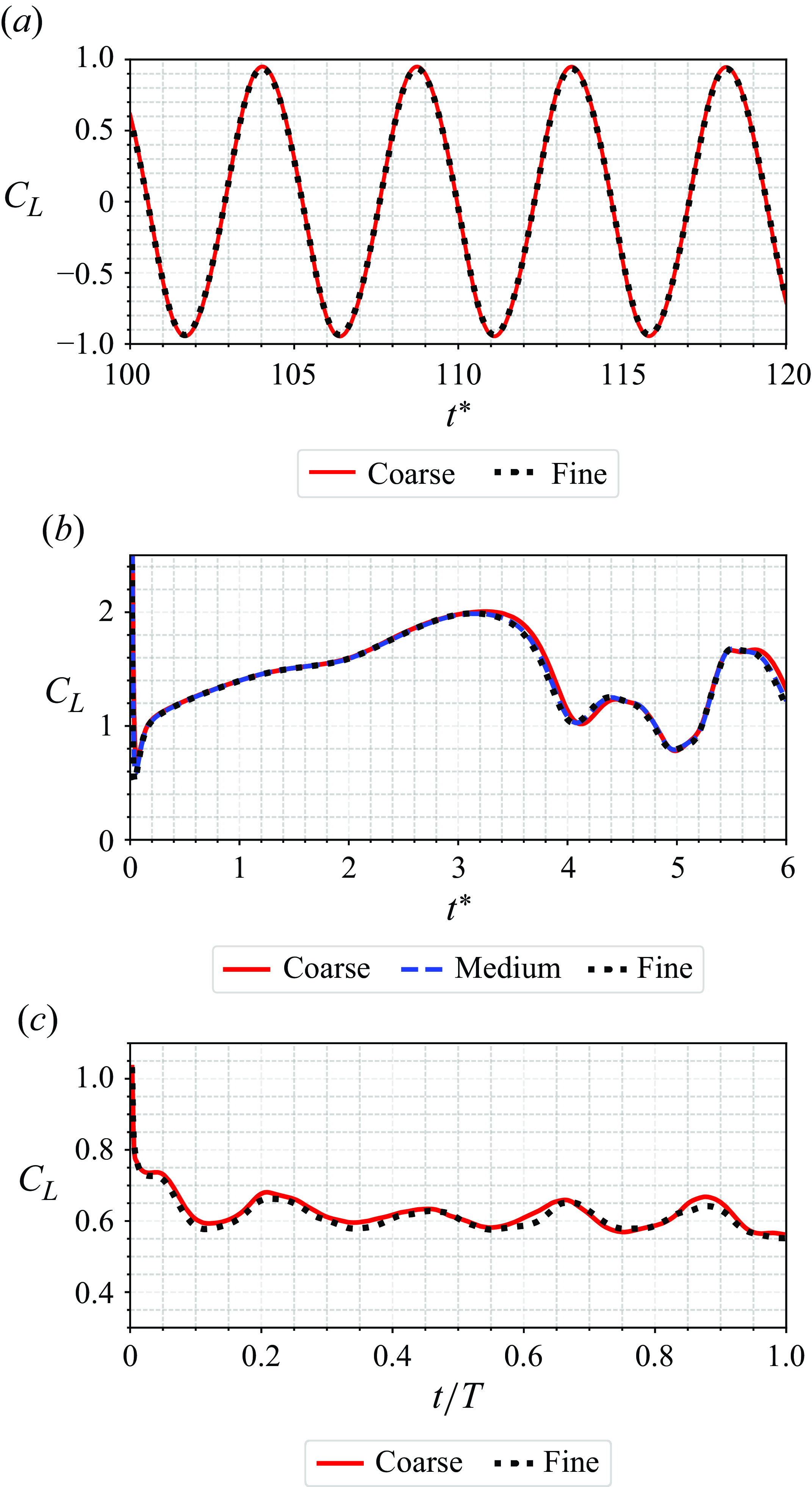
Figure 21. Grid convergence shown for (a) circular cylinder, (b) aerofoil and (c) revolving wing.
The grid convergence for the aerofoil is shown in figure 21(b), with the coarse, medium and fine meshes corresponding to 423 000, 665 000 and 960 000 grid points, respectively. The percentage difference between the RMS values of the lift coefficients between the coarse and medium grid sizes is 1.26 %, and this error reduces to 0.62 % between the medium and fine grid sizes. The medium grid is used for all the aerofoil results presented in this paper.
The grid convergence for the revolving wing is shown in figure 21(c), with the coarse and fine meshes containing approximately
 $9.6\times10^6$
and
$9.6\times10^6$
and
 $16\times10^6$
grid points, respectively. The RMS values of the lift coefficient between these two mesh differ by 1.61 %. The fine mesh is used for all the results presented in this paper.
$16\times10^6$
grid points, respectively. The RMS values of the lift coefficient between these two mesh differ by 1.61 %. The fine mesh is used for all the results presented in this paper.


 Open access