


1. Introduction
Rayleigh–Taylor (RT) instability arises when a lighter fluid supports a heavier fluid under the influence of gravity or when a lighter fluid accelerates against a heavier one (Rayleigh Reference Rayleigh1883; Taylor Reference Taylor1950). The acceleration field amplifies small perturbations on the fluid interface, driving the heavy and light fluids to interpenetrate, which eventually results in the development of turbulent flows. This phenomenon inherently produces a non-stationary, inhomogeneous and anisotropic flow, accompanied by an enhanced mixing process. The RT instability and its associated turbulence play a crucial role in numerous scientific and engineering applications, including supernova explosions (Hillebrandt & Niemeyer Reference Hillebrandt and Niemeyer2000; Wang & Chevalier Reference Wang and Chevalier2001; Zingale et al. Reference Zingale, Woosley, Rendleman, Day and Bell2005; Cabot & Cook Reference Cabot and Cook2006), the upwelling and overturning of stratified fluids (Tseng & Ferziger Reference Tseng and Ferziger2001; Cui & Street Reference Cui and Street2004), inertial confinement fusion (Amendt et al. Reference Amendt, Colvin, Tipton, Hinkel, Edwards, Landen, Ramshaw, Suter, Varnum and Watt2002; Betti & Hurricane Reference Betti and Hurricane2016; Zhang et al. Reference Zhang, Betti, Gopalaswamy, Yan and Aluie2018a ; Xin et al. Reference Xin, Yan, Wan, Sun, Zheng, Zhang, Aluie and Betti2019; Zhang et al. Reference Zhang, Betti, Yan and Aluie2020; Campbell et al. Reference Campbell2021) and combustion (Ashurst Reference Ashurst1996; Keenan, Makarov & Molkov Reference Keenan, Makarov and Molkov2014; Sykes, Gallagher & Rankin Reference Sykes, Gallagher and Rankin2021). Due to its significance and inherent complexities, the RT instability has been extensively studied through analytical, experimental and numerical approaches, which have been covered by several extensive reviews in recent years (Abarzhi Reference Abarzhi2010b ; Livescu Reference Livescu2013, Reference Livescu2020; Boffetta & Mazzino Reference Boffetta and Mazzino2017; Zhou Reference Zhou2017a ,Reference Zhou b ; Banerjee Reference Banerjee2020; Schilling Reference Schilling2020; Zhou et al. Reference Zhou, Feng, Hao and Li2021c ; Zhou, Sadler & Hurricane Reference Zhou, Sadler and Hurricane2025).
1.1. Non-stationary development of RT turbulence
During the early stages of RT instability, different modes composing the small initial perturbation at the interface between the two fluids grow exponentially and independently of each other, until they saturate when the perturbation amplitude becomes comparable to the wavelength of each mode. After this point, nonlinear interactions dominate, leading to the formation of coherent structures such as rising bubbles and sinking spikes. When initial perturbation is composed solely of high wavenumber components (Dimonte et al. Reference Dimonte2004), RT instability can enter a self-similar regime characterised by a quadratic temporal growth of the mixing width (Ristorcelli & Clark Reference Ristorcelli and Clark2004). Further evolution eventually leads to a transition to turbulence (Cook, Cabot & Miller Reference Cook, Cabot and Miller2004), significantly enhancing both energy transfer and material mixing rates. During the self-similar stage, including the fully turbulent phase, statistics such as growth rate, mixing rate and interfacial surface area follow stable power-law scalings with time, though some weak dependencies on the Reynolds number are observed (Cabot & Cook Reference Cabot and Cook2006).
Several phenomenological models have been proposed to explain the temporal behaviour of RT turbulence. Chertkov (Reference Chertkov2003) proposed a widely used model for three-dimensional (3-D) Boussinesq RT flows with negligible density variation, assuming that the release of potential energy, which primarily occurs at large scales, is slower compared with the energy transfer at intermediate to small scales. This model predicts that the integral length scale, velocity fluctuation in the inertial range and viscous length scale have power-law time dependences, and the forward energy cascade as well as the −5/3 scaling of energy spectrum can be established. This theory has been numerically confirmed (Boffetta et al. Reference Boffetta, Mazzino, Musacchio and Vozella2009; Matsumoto Reference Matsumoto2009) and subsequently extended by a Monin–Yaglom relation connecting the third-order structure function with the dissipation rate in RT turbulence (Soulard Reference Soulard2012). Other models, such as those proposed by Zhou (Reference Zhou2001); Poujade (Reference Poujade2006), and Abarzhi (Reference Abarzhi2010a ), predict different energy spectra scaling exponents based on different assumptions by incorporating varying levels of complexity of the flow physics. However, the time-dependent statistics is manifested in all these models, emphasising the statistically non-stationary nature of RT turbulence evolution.
There is currently no universal theory applicable to all RT turbulence configurations, due to the intrinsic challenges including its transient, inhomogeneous and variable-density nature. Furthermore, the diverse formulations used to describe RT systems, including the non-equilibrium discrete Boltzmann method (Xu et al. Reference Xu, Zhang, Gan, Chen and Yu2012; Lai et al. Reference Lai, Xu, Zhang, Gan, Ying and Succi2016; Chen, Xu & Zhang Reference Chen, Xu and Zhang2018; Zhang et al. Reference Zhang, Xu, Zhang, Li, Lai and Hu2021; Chen et al. Reference Chen, Xu, Chen, Zhang and Chen2022), the lattice Boltzmann method (He, Chen & Zhang Reference He, Chen and Zhang1999; Biferale et al. Reference Biferale, Mantovani, Sbragaglia, Scagliarini, Toschi and Tripiccione2010; Liang et al. Reference Liang, Li, Shi and Chai2016), compressible flows (Gauthier & Le Creurer Reference Gauthier and Le Creurer2010; Gauthier Reference Gauthier2017; Zhao, Liu & Lu Reference Zhao, Liu and Lu2020), incompressible variable-density flows (Cook & Zhou Reference Cook and Zhou2002; Livescu & Ristorcelli Reference Livescu and Ristorcelli2007, Reference Livescu and Ristorcelli2008) and the Boussinesq approximation (Boffetta et al. Reference Boffetta, Mazzino, Musacchio and Vozella2009; Matsumoto Reference Matsumoto2009; Boffetta & Mazzino Reference Boffetta and Mazzino2017), make it difficult to compare corresponding analytical or numerical results. In this paper we adopt a description based on miscible compressible fluids, and previous findings (Zhao et al. Reference Zhao, Liu and Lu2020; Zhou et al. Reference Zhou2021b ; Zhao, Betti & Aluie Reference Zhao, Betti and Aluie2022) indicate the existence of a Kolmogorov forward cascade for kinetic energy (KE) in such systems. We should note that when studying hydrodynamic instabilities involving very small scales or rarefied gases, such as interstellar plasmas, molecular fluctuations can be significant (Xu et al. Reference Xu, Zhang, Ying and Wang2016; Buttler, Williams & Najjar Reference Buttler, Williams and Najjar2017; Liu et al. Reference Liu, Song, Xu, Zhang and Xie2023; Zhang et al. Reference Zhang, Xu, Song, Gan, Zhang and Li2023; Majumder, Livescu & Girimaji Reference Majumder, Livescu and Girimaji2024). In these cases, the discrete Boltzmann method is more suitable for analysing the mixing process (Xu, Zhang & Gan Reference Xu, Zhang and Gan2024).
1.2. Multi-scale mixing statistics in RT turbulence
Initially, the concentration field in RT turbulence begins with pure heavy and light fluids segregated. Once the instability develops, the multi-scale velocity field distorts and stretches the interface between the fluids, increasing its surface area and enhancing molecular mixing at small scales. Consequently, mixing in RT turbulence emerges as a multi-scale process, driven by both small-scale mass diffusion and large-scale entrainment caused by the stirring effects of the velocity field (Villermaux Reference Villermaux2019).
Although the scalar or concentration field is transported by the fluid velocity, its multi-scale dynamics can differ significantly from those of the velocity field. For instance, the intermittency level of a passive scalar is generally found to be higher than that of the velocity field (Warhaft Reference Warhaft2000), and even a random Gaussian background velocity can induce non-Gaussian intermittency of the passive scalar field. Therefore, it is crucial to determine the multi-scale dynamics of the concentration field in RT turbulence and its connection with the velocity and the velocity gradient. An appropriate metric for quantifying the effects of multi-scale mixing should account for both large-scale entrainment and small-scale diffusion processes.
Previous research on RT mixing has primarily focused on single-point statistics, such as mixing width and the mixedness parameter. However, these averaged measures primarily reflect small-scale molecular mixing and do not adequately account for large-scale entrainment processes that can significantly enhance molecular mixing. For instance, the mixedness parameter is defined as $\Theta = \int _{-\infty }^\infty \langle X(1-X)\rangle _{xy} {\rm d}z/ \int _{-\infty }^\infty \langle X\rangle _{xy} \langle 1-X\rangle _{xy} {\rm d}z$
, where
$\Theta = \int _{-\infty }^\infty \langle X(1-X)\rangle _{xy} {\rm d}z/ \int _{-\infty }^\infty \langle X\rangle _{xy} \langle 1-X\rangle _{xy} {\rm d}z$
, where $X$
represents the mole fraction of the heavy or light fluid and
$X$
represents the mole fraction of the heavy or light fluid and $\langle \cdot \rangle _{xy}$
denotes an average over the horizontal plane. If only diffusion is active, with no convection, this parameter would equal 1 within a fully mixed region. Conversely, if only large-scale entrainment occurs without diffusion, the mole fraction field remains a rearrangement of pure fluids (only 0 or 1), resulting in
$\langle \cdot \rangle _{xy}$
denotes an average over the horizontal plane. If only diffusion is active, with no convection, this parameter would equal 1 within a fully mixed region. Conversely, if only large-scale entrainment occurs without diffusion, the mole fraction field remains a rearrangement of pure fluids (only 0 or 1), resulting in $\Theta$
being zero. Therefore, in the context of miscible RT turbulence, where the entrainment process is the initial step toward enhanced diffusion and molecular mixing, the mixedness parameter
$\Theta$
being zero. Therefore, in the context of miscible RT turbulence, where the entrainment process is the initial step toward enhanced diffusion and molecular mixing, the mixedness parameter $\Theta$
is inadequate for quantifying this multi-scale mixing process. Similarly, the probability density function (PDF) of the concentration and its associated moments (mean and variance) are also insufficient metrics, as the PDF remains unaffected by large-scale entrainment alone.
$\Theta$
is inadequate for quantifying this multi-scale mixing process. Similarly, the probability density function (PDF) of the concentration and its associated moments (mean and variance) are also insufficient metrics, as the PDF remains unaffected by large-scale entrainment alone.
Two-point statistics, which measures the inter-scale transfer of concentration, are more suitable for describing the multi-scale characteristics of mixing processes. For instance, inter-scale scalar transfer was studied by Yaglom et al. (Reference Yaglom1949), leading to the well-known 4/3 law for the structure function of passive scalars in homogeneous turbulence: $\langle \delta u_L(\boldsymbol {x};r) \delta \theta (\boldsymbol {x};r)^2\rangle = -4/3 \epsilon _\theta r$
, where
$\langle \delta u_L(\boldsymbol {x};r) \delta \theta (\boldsymbol {x};r)^2\rangle = -4/3 \epsilon _\theta r$
, where $\delta u_L(r), \delta \theta (r)$
are the longitudinal velocity increment and scalar increment across the separation length
$\delta u_L(r), \delta \theta (r)$
are the longitudinal velocity increment and scalar increment across the separation length $r$
,
$r$
, $\epsilon _\theta$
is the mean dissipation rate of scalar energy and
$\epsilon _\theta$
is the mean dissipation rate of scalar energy and $\langle \cdot \rangle$
represents spatial averaging. This result was later verified and extended to boundary layer flows (Danaila et al. Reference Danaila, Anselmet, Le Gal, Dusek, Brun and Pumir1997), turbulence at low Schmidt numbers (Iyer & Yeung Reference Iyer and Yeung2014) and grid-generated turbulence (Meyer, Mydlarski & Danaila Reference Meyer, Mydlarski and Danaila2018). Recently, Wang et al. (Reference Wang, Yurikusa, Iwano, Sakai, Ito, Zhou and Hattori2023) studied the nonlinear scalar transfer in grid-generated passive scalar turbulence with a mean scalar gradient perpendicular to the flow direction, using a Kármán–Howarth–Monin–Hill equation for the scalar increment. They found an inverse scalar energy transfer from small to large scales in the upstream region, driven by negative transfer along the scalar gradient direction, while in the downstream region, the transfer occurs from large to small scales. However, when the flow is driven parallel to the scalar gradient such as in RT flows, the mechanism of scalar transfer across different scales remains unclear. To the best of the authors’ knowledge, quantitative measurements of inter-scale scalar transfer, including point-split or filtering analyses of the concentration field budget, have not yet been considered for RT turbulence.
$\langle \cdot \rangle$
represents spatial averaging. This result was later verified and extended to boundary layer flows (Danaila et al. Reference Danaila, Anselmet, Le Gal, Dusek, Brun and Pumir1997), turbulence at low Schmidt numbers (Iyer & Yeung Reference Iyer and Yeung2014) and grid-generated turbulence (Meyer, Mydlarski & Danaila Reference Meyer, Mydlarski and Danaila2018). Recently, Wang et al. (Reference Wang, Yurikusa, Iwano, Sakai, Ito, Zhou and Hattori2023) studied the nonlinear scalar transfer in grid-generated passive scalar turbulence with a mean scalar gradient perpendicular to the flow direction, using a Kármán–Howarth–Monin–Hill equation for the scalar increment. They found an inverse scalar energy transfer from small to large scales in the upstream region, driven by negative transfer along the scalar gradient direction, while in the downstream region, the transfer occurs from large to small scales. However, when the flow is driven parallel to the scalar gradient such as in RT flows, the mechanism of scalar transfer across different scales remains unclear. To the best of the authors’ knowledge, quantitative measurements of inter-scale scalar transfer, including point-split or filtering analyses of the concentration field budget, have not yet been considered for RT turbulence.
By adopting the approach of scale decomposition and coarse graining, we can treat the diffusion process and large-scale entrainment on equal footing at coarse-grained levels. In this context, turbulent eddy diffusivity, which drives large-scale entrainment, plays a role analogous to molecular diffusivity at small scales. Several existing measures of mixing efficiency treat the reversible stirring and irreversible mixing equivalently, such as the coarse-grained density and segregation metrics in Krasnopolskaya et al. (Reference Krasnopolskaya, Meleshko, Peters and Meijer1999), and mixed norms or negative Sobolev norms in Mathew, Mezić & Petzold (Reference Mathew, Mezić and Petzold2005). However, these metrics are not directly connected to the underlying flow dynamics. In this paper we aim to describe the multi-scale mixing dynamics of RT turbulence directly through coarse-grained budget equations of the concentration field.
1.3. Anisotropy in RT turbulence
Anisotropy at various length scales is a key characteristic of RT turbulence. Due to the effects of external acceleration and the initial unstable stratification, the properties of RT turbulence in the vertical direction can differ significantly from those in the horizontal directions. Several metrics are used to quantify anisotropy in turbulent flows, the most common being vector component anisotropy, variance anisotropy and spectral anisotropy (Oughton et al. Reference Oughton, Matthaeus, Wan and Parashar2016). Vector component anisotropy refers to the unequal distribution among the three components of a vector field, while variance anisotropy is defined by the inequality among the diagonal elements of the variance tensor $\langle u_i u_j\rangle - \langle u_i\rangle \langle u_j\rangle$
for a vector field
$\langle u_i u_j\rangle - \langle u_i\rangle \langle u_j\rangle$
for a vector field $u_i$
. Both of these metrics describe directional anisotropy. In contrast, spectral anisotropy captures variations in spectral energy distribution when the components of the associated wavevector are varied independently (Shebalin, Matthaeus & Montgomery Reference Shebalin, Matthaeus and Montgomery1983; Oughton et al. Reference Oughton, Matthaeus, Wan and Parashar2016; Zhao & Aluie Reference Zhao and Aluie2023). This concept primarily quantifies differences in characteristic length scales associated with each spatial direction and can be seen as a form of shape anisotropy of the eddies related to any field variable. In this work we shall focus on the directional anisotropy at different length scales during RT evolution.
$u_i$
. Both of these metrics describe directional anisotropy. In contrast, spectral anisotropy captures variations in spectral energy distribution when the components of the associated wavevector are varied independently (Shebalin, Matthaeus & Montgomery Reference Shebalin, Matthaeus and Montgomery1983; Oughton et al. Reference Oughton, Matthaeus, Wan and Parashar2016; Zhao & Aluie Reference Zhao and Aluie2023). This concept primarily quantifies differences in characteristic length scales associated with each spatial direction and can be seen as a form of shape anisotropy of the eddies related to any field variable. In this work we shall focus on the directional anisotropy at different length scales during RT evolution.
In RT turbulence, vector component anisotropy has been studied by Cabot & Zhou (Reference Cabot and Zhou2013), who measured the differences between the components of various vector and tensor fields, including horizontally averaged velocity, vorticity and velocity derivatives. Their findings revealed that vertical velocity is significantly higher than horizontal velocity, while the behaviour of velocity derivatives differs between transverse and longitudinal components. Additionally, Cabot & Zhou (Reference Cabot and Zhou2013) analysed the one-dimensional longitudinal and transverse spectra for velocity and vorticity components, showing that while isotropy is observed at small scales, anisotropy becomes apparent at larger scales.
Similarly, variance anisotropy in RT turbulence can be quantified using the Reynolds stress anisotropic tensor, $b_{ij} = \langle u_i u_j \rangle / \langle |\boldsymbol {u}|^2 \rangle - ({1}/{3}) \delta _{ij}$
. A typical value of
$b_{ij} = \langle u_i u_j \rangle / \langle |\boldsymbol {u}|^2 \rangle - ({1}/{3}) \delta _{ij}$
. A typical value of $ b_{zz} = 0.3$
across the mixing layer is observed (Ristorcelli & Clark Reference Ristorcelli and Clark2004; Livescu et al. Reference Livescu, Ristorcelli, Gore, Dean, Cabot and Cook2009), indicating a dominance of vertical turbulent KE as a result of the vertical gravity injection. This measure has also been applied in Fourier space (Livescu et al. Reference Livescu, Ristorcelli, Gore, Dean, Cabot and Cook2009; Gauthier Reference Gauthier2017), where
$ b_{zz} = 0.3$
across the mixing layer is observed (Ristorcelli & Clark Reference Ristorcelli and Clark2004; Livescu et al. Reference Livescu, Ristorcelli, Gore, Dean, Cabot and Cook2009), indicating a dominance of vertical turbulent KE as a result of the vertical gravity injection. This measure has also been applied in Fourier space (Livescu et al. Reference Livescu, Ristorcelli, Gore, Dean, Cabot and Cook2009; Gauthier Reference Gauthier2017), where $b_{zz}(k)$
approaches zero at intermediate scales, suggesting isotropy, while anisotropy persists at both large and small scales due to the influence of buoyancy forcing. Most previous studies on RT turbulence have focused on the anisotropy of the velocity field, whereas research on the scalar field is relatively limited, primarily focusing on the anisotropy of length scales or spectra associated with the scalar field (Gauthier Reference Gauthier2017; Zhou & Cabot Reference Zhou and Cabot2019).
$b_{zz}(k)$
approaches zero at intermediate scales, suggesting isotropy, while anisotropy persists at both large and small scales due to the influence of buoyancy forcing. Most previous studies on RT turbulence have focused on the anisotropy of the velocity field, whereas research on the scalar field is relatively limited, primarily focusing on the anisotropy of length scales or spectra associated with the scalar field (Gauthier Reference Gauthier2017; Zhou & Cabot Reference Zhou and Cabot2019).
Understanding the directional anisotropy of RT turbulence is essential for developing numerical models used in large-eddy simulations (LES) or Reynolds-averaged Navier–Stokes (RANS) simulations for inhomogeneous and anisotropic turbulence. Traditional LES models such as the Smagorinsky model (Smagorinsky Reference Smagorinsky1963) or the nonlinear model (Clark, Ferziger & Reynolds Reference Clark, Ferziger and Reynolds1979), designed for isotropic turbulence, perform reasonably well in RT turbulence (Zhou et al. Reference Zhou, Feng, Hao and Li2021a ; Luo et al. Reference Luo, Wang, Yuan, Jiang, Huang and Wang2023) in terms of overall statistics. In the following sections we show that while a nonlinear model accurately captures the overall statistics of the scalar budget, it fails to predict the directional anisotropic behaviour. However, focusing exclusively on the fluctuating component of the scalar field (subtracting the horizontally averaged vertical profile) leads to improved predictions of anisotropy. This finding indicates that, in modelling RT turbulence, it is crucial to treat the horizontally averaged and fluctuating components separately.
The subsequent sections are organised as follows. Section 2 presents the governing equations and details of the numerical simulations. In § 3 we provide simulation results and the temporal evolution of RT mixing statistics. Section 4 delves into the scale transfer of the concentration field, examining its relationship with the strain rate and vorticity fields. In § 5 we analyse the directional anisotropy of KE and concentration, focusing particularly on the anisotropic behaviour of scalar variance transfer. Finally, § 6 summarises the physical mechanisms driving the multi-scale mixing process in RT turbulence and concludes the discussion.
2. Governing equations and numerical methods
We adopt the compressible miscible Navier–Stokes equations with two fluid species to describe the RT turbulent flow, including the conservation of mass, mass fraction, momentum and total energy (Gauthier Reference Gauthier2017; Zhao et al. Reference Zhao, Xiao, Aluie, Wei and Lin2023):
 \begin{eqnarray} & \dfrac {\partial \rho }{\partial t} + \nabla \cdot (\rho \boldsymbol {u}) = 0, \end{eqnarray}
 \begin{eqnarray} &\dfrac {\partial \rho Y_k}{\partial t} + \nabla \cdot (\rho \boldsymbol {u}Y_k) = \nabla \cdot (\rho D\nabla Y_k), \end{eqnarray}
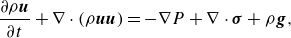 \begin{eqnarray} &\dfrac {\partial \rho \boldsymbol {u}}{\partial t} + \nabla \cdot (\rho \boldsymbol {u}\boldsymbol {u}) = -\nabla P+\nabla \cdot \boldsymbol {\sigma }+\rho \boldsymbol {g}, \end{eqnarray}
 \begin{eqnarray} &\dfrac {\partial \rho E}{\partial t} + \nabla \cdot ((\rho E + P)\boldsymbol {u}) = \nabla \cdot (\boldsymbol {\sigma }\cdot \boldsymbol {u}) +\rho \boldsymbol {u}\cdot \boldsymbol {g} - \nabla \cdot \boldsymbol {q}. \end{eqnarray}
Here $\rho , \boldsymbol {u}, P$
are the density, velocity and pressure fields, respectively,
$\rho , \boldsymbol {u}, P$
are the density, velocity and pressure fields, respectively, $\boldsymbol {g}=(0, 0, -g)$
is the gravitational acceleration along the negative vertical direction,
$\boldsymbol {g}=(0, 0, -g)$
is the gravitational acceleration along the negative vertical direction, $Y_k$
is the mass fraction of the
$Y_k$
is the mass fraction of the $k$
th component,
$k$
th component, $k=h$
and
$k=h$
and $l$
for heavy and light fluids respectively, and
$l$
for heavy and light fluids respectively, and $E= ({1}/{2})u^2 + c_v T$
is the total energy density, in which
$E= ({1}/{2})u^2 + c_v T$
is the total energy density, in which $c_v$
is the specific heat at constant volume and
$c_v$
is the specific heat at constant volume and $T$
is temperature.
$T$
is temperature. $\boldsymbol {q}=-\kappa \nabla T$
is the heat flux vector,
$\boldsymbol {q}=-\kappa \nabla T$
is the heat flux vector, $\boldsymbol {\sigma }=2\mu (\mathbf {S}-({1}/{3})\mathrm {tr}(\mathbf {S})\mathbf {I})$
is the viscous stress tensor,
$\boldsymbol {\sigma }=2\mu (\mathbf {S}-({1}/{3})\mathrm {tr}(\mathbf {S})\mathbf {I})$
is the viscous stress tensor, $\mathbf {S}=(\nabla \boldsymbol {u}+\nabla \boldsymbol {u}^T)/2$
is the strain rate tensor,
$\mathbf {S}=(\nabla \boldsymbol {u}+\nabla \boldsymbol {u}^T)/2$
is the strain rate tensor, $\mathbf {I}$
is the identity tensor and
$\mathbf {I}$
is the identity tensor and $\mu , D,\kappa$
are the dynamic viscosity, mass diffusivity and thermal conductivity, respectively.
$\mu , D,\kappa$
are the dynamic viscosity, mass diffusivity and thermal conductivity, respectively.
The above set of equations is complemented by the ideal gas equation of state, $P=\rho \widetilde {R} T (Y_h/W_h + Y_l/W_l)$
, where
$P=\rho \widetilde {R} T (Y_h/W_h + Y_l/W_l)$
, where $\widetilde {R}$
is the universal gas constant,
$\widetilde {R}$
is the universal gas constant, $W_h, W_l$
are the molecular weights of the two species. By setting equal molecular weights
$W_h, W_l$
are the molecular weights of the two species. By setting equal molecular weights $W_h=W_l=W$
, the ideal gas equation of state reduces to
$W_h=W_l=W$
, the ideal gas equation of state reduces to $P=\rho ({\widetilde {R}}/{W}) T$
, and the mass fraction equation (2.2) is thus decoupled from other equations and acts as a passive scalar. Additionally, due to the constraint
$P=\rho ({\widetilde {R}}/{W}) T$
, and the mass fraction equation (2.2) is thus decoupled from other equations and acts as a passive scalar. Additionally, due to the constraint $Y_h + Y_l = 1$
, only one of the mass fraction equations (2.2) is required to solve the system. Henceforth, unless otherwise stated, we use
$Y_h + Y_l = 1$
, only one of the mass fraction equations (2.2) is required to solve the system. Henceforth, unless otherwise stated, we use $Y$
to denote the mass fraction of the heavy fluid.
$Y$
to denote the mass fraction of the heavy fluid.
The computational domain is a rectangular box with dimensions of $L_x \times L_y \times L_z = 0.8 \times 0.8 \times 1.6$
, containing an isopycnal initial density profile. In this set-up, the upper half of the domain is filled with a uniform heavy fluid of density
$L_x \times L_y \times L_z = 0.8 \times 0.8 \times 1.6$
, containing an isopycnal initial density profile. In this set-up, the upper half of the domain is filled with a uniform heavy fluid of density $\rho _h$
and the lower half with a light fluid of density
$\rho _h$
and the lower half with a light fluid of density $\rho _l$
. Consequently, the mass fraction of the heavy fluid is
$\rho _l$
. Consequently, the mass fraction of the heavy fluid is $Y = 1$
in the upper half and
$Y = 1$
in the upper half and $Y=0$
in the lower half, with the corresponding Atwood number given by
$Y=0$
in the lower half, with the corresponding Atwood number given by $\mathrm {At}=(\rho _h - \rho _l) / (\rho _h + \rho _l)$
. The initial pressure field satisfies the hydrostatic condition
$\mathrm {At}=(\rho _h - \rho _l) / (\rho _h + \rho _l)$
. The initial pressure field satisfies the hydrostatic condition $\partial P/\partial z= -\rho g$
and the initial temperature is derived from the ideal gas equation of state. An initial perturbation is applied to the vertical velocity field near the interface between the heavy and light fluids, with energy distributed equally across the wavenumber shells
$\partial P/\partial z= -\rho g$
and the initial temperature is derived from the ideal gas equation of state. An initial perturbation is applied to the vertical velocity field near the interface between the heavy and light fluids, with energy distributed equally across the wavenumber shells $k \in [32, 64]$
, corresponding to the bubble merger regime in RT turbulence. Boundary conditions are periodic in the horizontal directions, with no-slip walls at the top and bottom boundaries. The temperature and mass fraction fields have zero-gradient boundary conditions at the top and bottom walls. The system of equations (2.1)–(2.4) is solved numerically using a pseudo-spectral method in the horizontal direction and a sixth-order compact finite difference scheme in the vertical direction. To prevent contamination from high wavenumbers due to nonlinearity, the 2/3 dealiasing rule (Patterson & Orszag Reference Patterson and Orszag1971) and a compact filtering scheme (Lele Reference Lele1992; Brady & Livescu Reference Brady and Livescu2019) are applied. Further details can be found in Zhao et al. (Reference Zhao, Betti and Aluie2022).
$k \in [32, 64]$
, corresponding to the bubble merger regime in RT turbulence. Boundary conditions are periodic in the horizontal directions, with no-slip walls at the top and bottom boundaries. The temperature and mass fraction fields have zero-gradient boundary conditions at the top and bottom walls. The system of equations (2.1)–(2.4) is solved numerically using a pseudo-spectral method in the horizontal direction and a sixth-order compact finite difference scheme in the vertical direction. To prevent contamination from high wavenumbers due to nonlinearity, the 2/3 dealiasing rule (Patterson & Orszag Reference Patterson and Orszag1971) and a compact filtering scheme (Lele Reference Lele1992; Brady & Livescu Reference Brady and Livescu2019) are applied. Further details can be found in Zhao et al. (Reference Zhao, Betti and Aluie2022).
In the subsequent sections we adopt the coarse-graining approach to decompose turbulence fields into different scales. Coarse graining applied to any 3-D field $f(\boldsymbol {x})$
is a low-pass filtering defined by a convolution
$f(\boldsymbol {x})$
is a low-pass filtering defined by a convolution
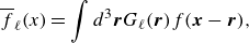 \begin{align} \overline {f}_\ell (x) = \int d^3{\boldsymbol {r}} G_\ell ({\boldsymbol {r}}) f(\boldsymbol {x}-{\boldsymbol {r}}), \end{align}
where the normalised kernel $G_\ell ({\boldsymbol {r}}) = \ell ^{-3} G({\boldsymbol {r}}/\ell )$
is a dilated kernel with a characteristic width
$G_\ell ({\boldsymbol {r}}) = \ell ^{-3} G({\boldsymbol {r}}/\ell )$
is a dilated kernel with a characteristic width $\ell$
. The coarse graining defined in (2.5) decomposes the field
$\ell$
. The coarse graining defined in (2.5) decomposes the field $f(\boldsymbol {x})$
into a large-scale (
$f(\boldsymbol {x})$
into a large-scale ( $\gtrapprox \ell$
) component
$\gtrapprox \ell$
) component $\overline {f}_\ell$
and a small-scale (
$\overline {f}_\ell$
and a small-scale ( $\lessapprox \ell$
) component
$\lessapprox \ell$
) component $f_\ell ^{\prime}=f-\overline {f}_\ell$
. This approach is widely adopted in LES to separate the resolved-scale and subgrid-scale dynamics (Meneveau & Katz Reference Meneveau and Katz2000a
), and the Gaussian filter, due to its positivity in both physical and Fourier spaces, is commonly adopted as the filtering kernel. Since the Gaussian filter is separable, for isotropic filtering in Cartesian coordinates, we adopt
$f_\ell ^{\prime}=f-\overline {f}_\ell$
. This approach is widely adopted in LES to separate the resolved-scale and subgrid-scale dynamics (Meneveau & Katz Reference Meneveau and Katz2000a
), and the Gaussian filter, due to its positivity in both physical and Fourier spaces, is commonly adopted as the filtering kernel. Since the Gaussian filter is separable, for isotropic filtering in Cartesian coordinates, we adopt
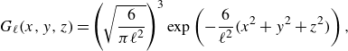 \begin{align} G_\ell (x,y,z)=\left (\sqrt {\frac {6}{\pi \ell ^2}}\right )^3 \exp \left ( -\frac {6}{\ell ^2} (x^2+y^2+z^2)\right ), \end{align}
where the filtering width is the same along the three Cartesian coordinates.
In complex flows such as RT turbulence, special treatment is needed for coarse graining near walls. We extend the domain beyond the physical boundaries with values consistent with the boundary conditions. For RT flows, the velocity is set to zero beyond the walls, the density and mass fraction fields are held constant due to zero-gradient conditions, while the extended pressure field satisfies the hydrostatic condition ${\rm d}P/{\rm d}z=-\rho g$
(Zhao & Aluie Reference Zhao and Aluie2018; Zhao et al. Reference Zhao, Betti and Aluie2022). This approach enables filtering throughout the domain without resorting to inhomogeneous filtering near the wall.
${\rm d}P/{\rm d}z=-\rho g$
(Zhao & Aluie Reference Zhao and Aluie2018; Zhao et al. Reference Zhao, Betti and Aluie2022). This approach enables filtering throughout the domain without resorting to inhomogeneous filtering near the wall.
3. Temporal evolution of mixing statistics
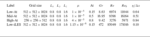
We perform numerical simulations of RT turbulence at low- to high-Atwood numbers, with $\mathrm {At}=(\rho _h-\rho _l)/(\rho _h+\rho _l)=0.15$
,
$\mathrm {At}=(\rho _h-\rho _l)/(\rho _h+\rho _l)=0.15$
, $0.5$
and
$0.5$
and $0.8$
, respectively. The parameters are shown in table 1. All simulations have a spatially uniform dynamic viscosity
$0.8$
, respectively. The parameters are shown in table 1. All simulations have a spatially uniform dynamic viscosity $\mu$
and unity Prandtl number
$\mu$
and unity Prandtl number $\mathrm {Pr}=c_p \mu /\kappa =1$
, with
$\mathrm {Pr}=c_p \mu /\kappa =1$
, with $\kappa$
the thermal conductivity and
$\kappa$
the thermal conductivity and $c_p=2$
the specific heat capacity at constant pressure. The grid size is checked to satisfy the criterion for adequate resolution of the smallest scales,
$c_p=2$
the specific heat capacity at constant pressure. The grid size is checked to satisfy the criterion for adequate resolution of the smallest scales, $k_{\mathrm {max}}\eta \geqslant 1.5$
(Yeung & Pope Reference Yeung and Pope1989), where
$k_{\mathrm {max}}\eta \geqslant 1.5$
(Yeung & Pope Reference Yeung and Pope1989), where $k_{\mathrm {max}}$
is the maximum resolved wavenumber and
$k_{\mathrm {max}}$
is the maximum resolved wavenumber and $\eta =\mu ^{3/4}/(\epsilon ^{1/4}\langle \rho \rangle ^{3/4})$
is the Kolmogorov scale. The temporal evolution of the Kolmogorov scale
$\eta =\mu ^{3/4}/(\epsilon ^{1/4}\langle \rho \rangle ^{3/4})$
is the Kolmogorov scale. The temporal evolution of the Kolmogorov scale $\eta$
is shown in figure 16 in Appendix A, indicating an adequate resolution during the time span studied in this paper. In the following sections we primarily focus on the low- and mid-At cases. However, for completeness and verification purposes, we have also added two additional simulations: one labelled high-At for a simulation at
$\eta$
is shown in figure 16 in Appendix A, indicating an adequate resolution during the time span studied in this paper. In the following sections we primarily focus on the low- and mid-At cases. However, for completeness and verification purposes, we have also added two additional simulations: one labelled high-At for a simulation at $\mathrm {At}=0.8$
and another labelled low-iLES for an implicit LES performed at
$\mathrm {At}=0.8$
and another labelled low-iLES for an implicit LES performed at $\mathrm {At}=0.15$
. The implicit LES simulation, which solves the same set of equations (2.1)–(2.4) on an under-resolved grid, satisfies the mixing transition criterion for RT turbulence (Zhou, Robey & Buckingham Reference Zhou, Robey and Buckingham2003; Qi et al. Reference Qi, He, Xu and Zhang2024; Xiao, Qi & Zhang Reference Xiao, Qi and Zhang2025; Xie et al. Reference Xie, Qi, Xiao, Zhang and Zhao2025) for outer-scale Reynolds numbers greater than
$\mathrm {At}=0.15$
. The implicit LES simulation, which solves the same set of equations (2.1)–(2.4) on an under-resolved grid, satisfies the mixing transition criterion for RT turbulence (Zhou, Robey & Buckingham Reference Zhou, Robey and Buckingham2003; Qi et al. Reference Qi, He, Xu and Zhang2024; Xiao, Qi & Zhang Reference Xiao, Qi and Zhang2025; Xie et al. Reference Xie, Qi, Xiao, Zhang and Zhao2025) for outer-scale Reynolds numbers greater than $1.6 \times 10^5$
. In Appendix E we verify that the main results for the low- and mid-At cases are also applicable to the high-At and low-iLES cases.
$1.6 \times 10^5$
. In Appendix E we verify that the main results for the low- and mid-At cases are also applicable to the high-At and low-iLES cases.
Table 1. Parameters of the RT simulations conducted in this study. The domain lengths in the three directions are denoted by $L_x$
,
$L_x$
, $L_y$
and
$L_y$
and $L_z$
, and
$L_z$
, and $\mathrm {At}$
represents the Atwood number. Gravitational acceleration is set to
$\mathrm {At}$
represents the Atwood number. Gravitational acceleration is set to $g=1$
in the
$g=1$
in the $-z$
direction. The mesh Grashof number is defined as
$-z$
direction. The mesh Grashof number is defined as $Gr=2\mathrm {At}\ g\langle \rho \rangle ^2 \Delta x^3/\mu ^2$
, the Kolmogorov scale as
$Gr=2\mathrm {At}\ g\langle \rho \rangle ^2 \Delta x^3/\mu ^2$
, the Kolmogorov scale as $\eta =\mu ^{3/4}/(\epsilon ^{1/4}\langle \rho \rangle ^{3/4})$
and the Reynolds number as
$\eta =\mu ^{3/4}/(\epsilon ^{1/4}\langle \rho \rangle ^{3/4})$
and the Reynolds number as $Re=\langle |\boldsymbol {u}|^2\rangle ^{1/2} L_x\langle \rho \rangle /\mu$
, where
$Re=\langle |\boldsymbol {u}|^2\rangle ^{1/2} L_x\langle \rho \rangle /\mu$
, where $\langle \cdot \rangle$
denotes the spatial mean over the whole simulation domain and
$\langle \cdot \rangle$
denotes the spatial mean over the whole simulation domain and $\epsilon$
is the KE dissipation rate. The outer-scale Reynolds number is defined as
$\epsilon$
is the KE dissipation rate. The outer-scale Reynolds number is defined as $Re_h= \langle \rho \rangle h\dot {h}/\mu$
, where
$Re_h= \langle \rho \rangle h\dot {h}/\mu$
, where $h(t)$
is the mixing width defined in (3.1). The mass diffusivity
$h(t)$
is the mixing width defined in (3.1). The mass diffusivity $D$
is set to be equal to the dynamic viscosity
$D$
is set to be equal to the dynamic viscosity $\mu$
. In the table, the Reynolds number and Kolmogorov scale are calculated at the dimensionless time
$\mu$
. In the table, the Reynolds number and Kolmogorov scale are calculated at the dimensionless time $\widehat {t}=t/\sqrt { ({L_x}/{\mathrm {At})\ g}}=5.0$
.
$\widehat {t}=t/\sqrt { ({L_x}/{\mathrm {At})\ g}}=5.0$
.
3.1. Evolution of the mixing layer
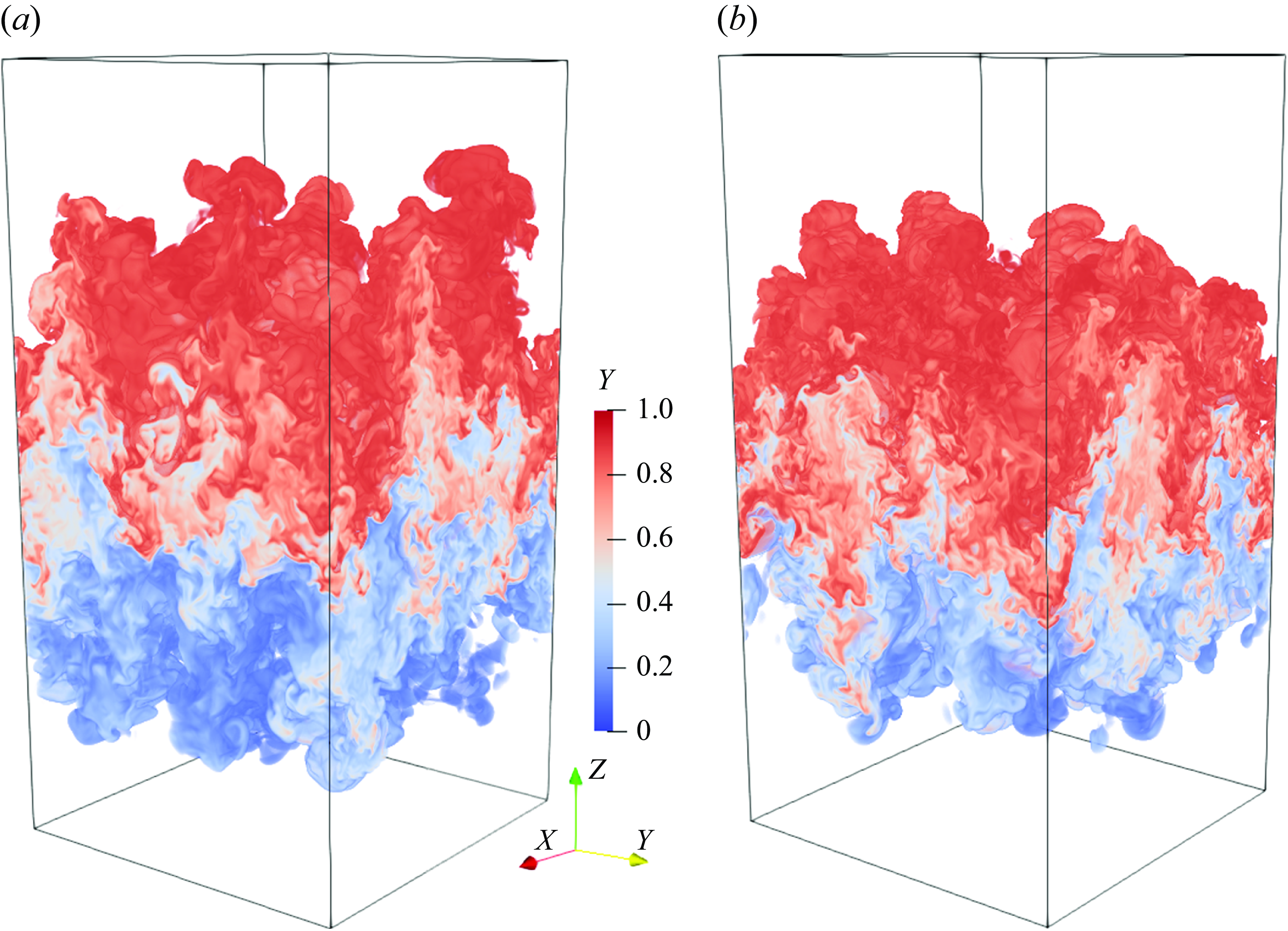
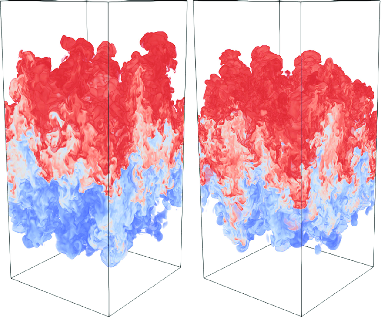
Figure 1. Visualisations of the mass fraction fields $Y$
at dimensionless time
$Y$
at dimensionless time $\widehat {t}=t \sqrt {\mathrm {At} g/L_x}=4.5$
for (a) low-At case at
$\widehat {t}=t \sqrt {\mathrm {At} g/L_x}=4.5$
for (a) low-At case at $\mathrm {At}=0.15$
, and (b) mid-At case at
$\mathrm {At}=0.15$
, and (b) mid-At case at $\mathrm {At}=0.5$
.
$\mathrm {At}=0.5$
.
Figure 1 shows the visualisations of the mass fraction fields $Y$
for the low-At and mid-At cases at dimensionless time
$Y$
for the low-At and mid-At cases at dimensionless time $\widehat {t} = t\sqrt {\mathrm {At} g/L_x}=4.5$
, where
$\widehat {t} = t\sqrt {\mathrm {At} g/L_x}=4.5$
, where $\sqrt {L_x/(\mathrm {At} g)}$
is the characteristic time scale of RT flows. The flow encompasses a wide range of length scales, and the mixing zone heights are similar for the two cases. A quantitative measure of the mixing zone growth is the mixing width
$\sqrt {L_x/(\mathrm {At} g)}$
is the characteristic time scale of RT flows. The flow encompasses a wide range of length scales, and the mixing zone heights are similar for the two cases. A quantitative measure of the mixing zone growth is the mixing width $h(t)$
, defined as (Cabot & Cook Reference Cabot and Cook2006; Zhang et al. Reference Zhang, Betti, Yan, Zhao, Shvarts and Aluie2018b
)
$h(t)$
, defined as (Cabot & Cook Reference Cabot and Cook2006; Zhang et al. Reference Zhang, Betti, Yan, Zhao, Shvarts and Aluie2018b
)
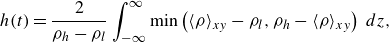 \begin{align} h(t)=\frac {2}{\rho _h-\rho _l} \int _{-\infty }^\infty \mathrm {min}\left (\langle \rho \rangle _{xy}-\rho _l, \rho _h-\langle \rho \rangle _{xy}\right )\ {\rm d}z, \end{align}
where $\langle \cdot \rangle _{xy}=( {1}/{L_x L_y}) \iint (\cdot ){\rm d}x {\rm d}y$
is a horizontally averaged quantity (a function of
$\langle \cdot \rangle _{xy}=( {1}/{L_x L_y}) \iint (\cdot ){\rm d}x {\rm d}y$
is a horizontally averaged quantity (a function of $z$
) and
$z$
) and $\rho _l, \rho _h$
are densities of the light and heavy fluids. In figure 2(a) the mixing width exhibits quadratic growth with time for both cases after
$\rho _l, \rho _h$
are densities of the light and heavy fluids. In figure 2(a) the mixing width exhibits quadratic growth with time for both cases after $\widehat {t}\gt 2$
, suggesting a self-similar expansion of the RT mixing zone. The fitted growth rate coefficient
$\widehat {t}\gt 2$
, suggesting a self-similar expansion of the RT mixing zone. The fitted growth rate coefficient $\alpha$
, appearing in the quadratic growth expression
$\alpha$
, appearing in the quadratic growth expression $h(t) = \alpha \mathrm {At}\,gt^2$
, is 0.0232 for the low-At case and 0.0209 for the mid-At case, both of which fall within the range reported in the literature (Zhou 2017a).
$h(t) = \alpha \mathrm {At}\,gt^2$
, is 0.0232 for the low-At case and 0.0209 for the mid-At case, both of which fall within the range reported in the literature (Zhou 2017a).
A related metric is the mixedness parameter, $\Theta$
(see introduction), which measures the degree of molecular mixing along horizontal planes and is defined as
$\Theta$
(see introduction), which measures the degree of molecular mixing along horizontal planes and is defined as
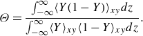 \begin{align} \Theta = \frac {\int _{-\infty }^\infty \langle Y(1-Y)\rangle _{xy} {\rm d}z}{\int _{-\infty }^\infty \langle Y\rangle _{xy} \langle 1-Y\rangle _{xy} {\rm d}z}. \end{align}
The parameter $\Theta$
is intended to measure the rate of reaction in a mixture, in which the molar fraction shall be adopted in the above definition instead of mass fraction (Youngs Reference Youngs1991; Wilson & Andrews Reference Wilson and Andrews2002). Here in our RT configuration, the molecular weights of the two fluids are assumed to be equal, so the mass fraction is equal to the molar fraction, making the use of the above definition appropriate.
$\Theta$
is intended to measure the rate of reaction in a mixture, in which the molar fraction shall be adopted in the above definition instead of mass fraction (Youngs Reference Youngs1991; Wilson & Andrews Reference Wilson and Andrews2002). Here in our RT configuration, the molecular weights of the two fluids are assumed to be equal, so the mass fraction is equal to the molar fraction, making the use of the above definition appropriate.
Figure 2(b) shows that initially, the presence of a small transition region near the fluid interface results in well-mixed flow within this region, leading to $\Theta \approx 1$
. The parameter stays around 1 for
$\Theta \approx 1$
. The parameter stays around 1 for $\widehat {t}\lt 1$
during which the diffusion effect is dominant and the instability has yet to grow. After this transient period, the instability grows and the fluid is dominated by advection. The fluid interface stretches and folds, causing large regions of unmixed pure fluids to be entrained into the mixing zone, which reduces the mixedness parameter
$\widehat {t}\lt 1$
during which the diffusion effect is dominant and the instability has yet to grow. After this transient period, the instability grows and the fluid is dominated by advection. The fluid interface stretches and folds, causing large regions of unmixed pure fluids to be entrained into the mixing zone, which reduces the mixedness parameter $\Theta$
. As the entrainment process progresses, the interfacial area increases, enhancing diffusion at these interfaces, which is reflected by a subsequent rise in
$\Theta$
. As the entrainment process progresses, the interfacial area increases, enhancing diffusion at these interfaces, which is reflected by a subsequent rise in $\Theta$
between
$\Theta$
between $1.5 \leqslant \widehat {t} \leqslant 2$
. After
$1.5 \leqslant \widehat {t} \leqslant 2$
. After $\widehat {t} \gt 2$
, the effect of advection and entrainment of pure fluids (which decreases
$\widehat {t} \gt 2$
, the effect of advection and entrainment of pure fluids (which decreases $\Theta$
) balances with the effect of interface diffusion (which increases
$\Theta$
) balances with the effect of interface diffusion (which increases $\Theta$
), leading to a saturation of
$\Theta$
), leading to a saturation of $\Theta$
around 0.8, consistent with results in Cook et al. (Reference Cook, Cabot and Miller2004); Banerjee & Andrews (Reference Banerjee and Andrews2009).
$\Theta$
around 0.8, consistent with results in Cook et al. (Reference Cook, Cabot and Miller2004); Banerjee & Andrews (Reference Banerjee and Andrews2009).
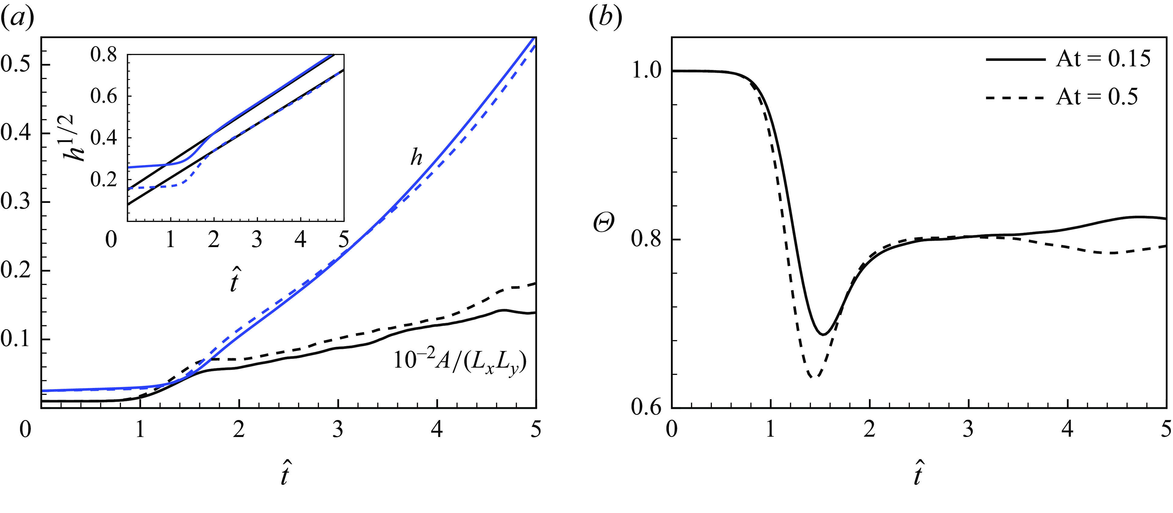
Figure 2. Evolution of (a) the total mixing width $h$
and the area
$h$
and the area $A/(L_xL_y)$
, and (b) the mixedness parameter
$A/(L_xL_y)$
, and (b) the mixedness parameter $\Theta$
of the isosurface
$\Theta$
of the isosurface $Y=0.5$
for the low-At and mid-At simulation cases. In the inset of panel (a), the square root of the mixing width is depicted to measure the growth coefficient
$Y=0.5$
for the low-At and mid-At simulation cases. In the inset of panel (a), the square root of the mixing width is depicted to measure the growth coefficient $\alpha$
corresponding to the quadratic growth rate
$\alpha$
corresponding to the quadratic growth rate $h(t)=\alpha \mathrm {At}gt^2$
marked by the black solid lines. The low-At case in the inset is shifted upward by 0.1 to distinguish it from the mid-At case, and the corresponding
$h(t)=\alpha \mathrm {At}gt^2$
marked by the black solid lines. The low-At case in the inset is shifted upward by 0.1 to distinguish it from the mid-At case, and the corresponding $\alpha$
values are 0.0232 and 0.0209 for the low-At and mid-At cases, respectively. Throughout this work, solid and dashed lines represent the low-At and mid-At cases, respectively, unless otherwise specified.
$\alpha$
values are 0.0232 and 0.0209 for the low-At and mid-At cases, respectively. Throughout this work, solid and dashed lines represent the low-At and mid-At cases, respectively, unless otherwise specified.
To further reveal the roles of advection and diffusion, in figure 2(a) we also show the evolution of the normalised area $A/(L_xL_y)$
of the
$A/(L_xL_y)$
of the $Y=0.5$
isosurface, obtained using the marching cube algorithm (Lorensen & Cline Reference Lorensen and Cline1998). The algorithm divides space into voxels (small cubes), interpolates isosurface intersections along their edges and connects these points based on vertex positions to form a piecewise-linear isosurface approximation. In accordance with the evolution of the mixedness
$Y=0.5$
isosurface, obtained using the marching cube algorithm (Lorensen & Cline Reference Lorensen and Cline1998). The algorithm divides space into voxels (small cubes), interpolates isosurface intersections along their edges and connects these points based on vertex positions to form a piecewise-linear isosurface approximation. In accordance with the evolution of the mixedness $\Theta$
, the isosurface areas are close to flat with a value of
$\Theta$
, the isosurface areas are close to flat with a value of $L_xL_y$
during
$L_xL_y$
during $\widehat {t}\lt 1$
, while they increase rapidly within
$\widehat {t}\lt 1$
, while they increase rapidly within $1\lt \widehat {t}\lt 1.5$
and the growths are close to exponential, similar to the area increase of a material surface in isotropic turbulence (Batchelor Reference Batchelor1952). After
$1\lt \widehat {t}\lt 1.5$
and the growths are close to exponential, similar to the area increase of a material surface in isotropic turbulence (Batchelor Reference Batchelor1952). After $\widehat {t}\gt 1.5$
, the enhanced diffusional effect hinders the growth of the isosurface area, and the exponential growth rate shifts towards a nearly linear growth in time after
$\widehat {t}\gt 1.5$
, the enhanced diffusional effect hinders the growth of the isosurface area, and the exponential growth rate shifts towards a nearly linear growth in time after $\widehat {t}\gt 2$
, during which the system is self-similar and the mixedness parameter remains roughly constant.
$\widehat {t}\gt 2$
, during which the system is self-similar and the mixedness parameter remains roughly constant.
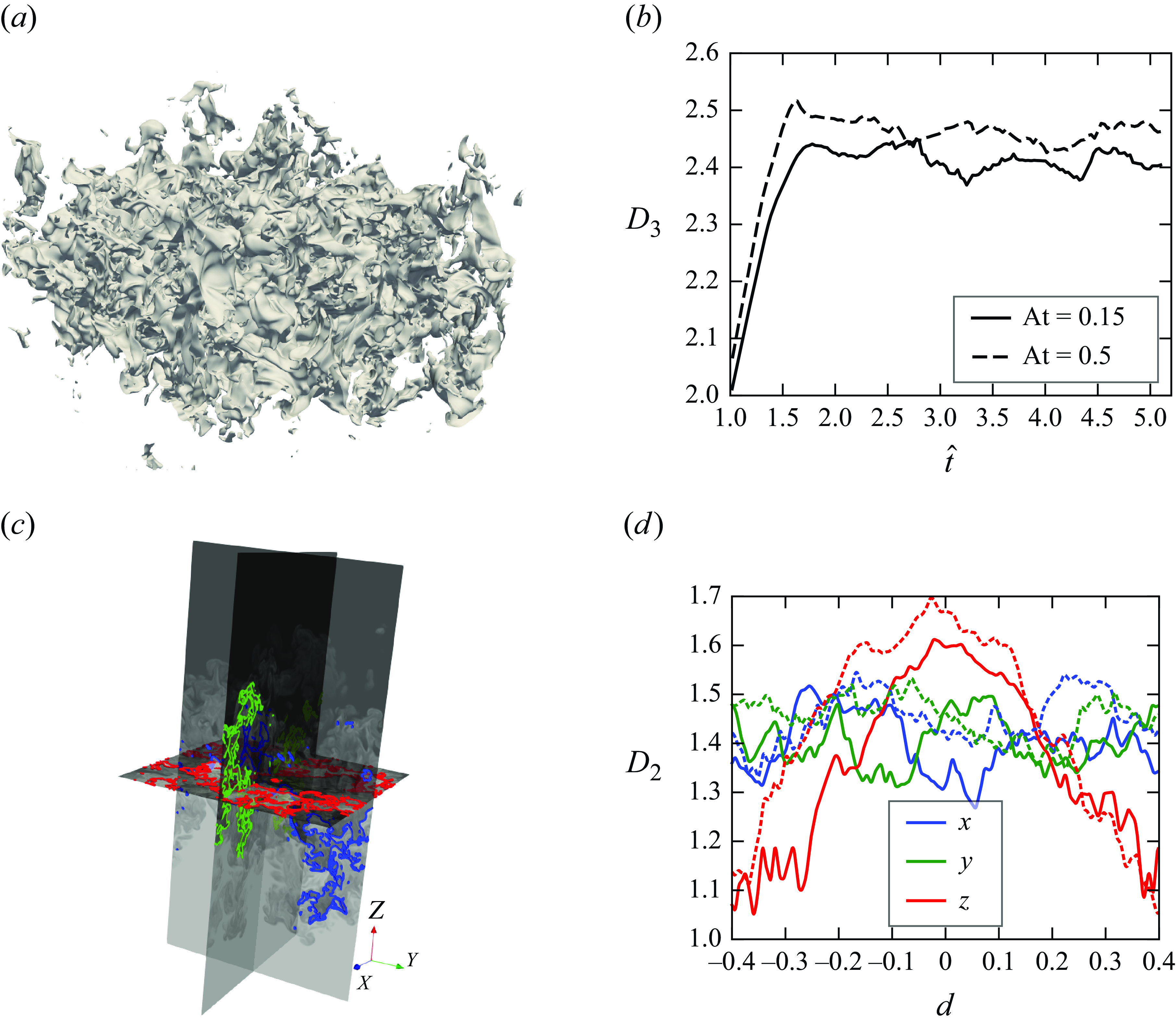
Figure 3. (a) Visualisation of the isosurface of the low-At case at $\widehat {t}=5$
. (b) The temporal evolution of the fractal dimension
$\widehat {t}=5$
. (b) The temporal evolution of the fractal dimension $D_3$
of the isosurfaces, measured with the box-counting algorithm (Mandelbrot Reference Mandelbrot1982). (c) Visualisation of isolines on three 2-D slices along the
$D_3$
of the isosurfaces, measured with the box-counting algorithm (Mandelbrot Reference Mandelbrot1982). (c) Visualisation of isolines on three 2-D slices along the $x$
-,
$x$
-, $y$
-, and
$y$
-, and $z$
-normal directions for the low-At case at
$z$
-normal directions for the low-At case at $\widehat {t}=5$
. (d) The fractal dimension
$\widehat {t}=5$
. (d) The fractal dimension $D_2$
of the isolines at different slice locations
$D_2$
of the isolines at different slice locations $d$
, where
$d$
, where $d$
denotes the
$d$
denotes the $x$
,
$x$
, $y$
, or
$y$
, or $z$
location of the slices relative to the domain centre. The low-At cases are shown in solid lines, while the mid-At cases are in dashed lines.
$z$
location of the slices relative to the domain centre. The low-At cases are shown in solid lines, while the mid-At cases are in dashed lines.
Unlike the mixing width, the interfacial area of the mid-At case is consistently larger than that of the low-At case, suggesting that the isosurface is more wrinkled with a greater heavy--light density contrast, and therefore, more potential energy is injected into the system. A quantitative measure of these interfacial topologies, shown in figure 3(a) for isosurfaces or figure 3(c) for cross-sectional isolines, is the fractal dimension, $D_3$
and
$D_3$
and $D_2$
, embedded in 3-D and two-dimensional (2-D) space, respectively. The fractal dimension is calculated using the box-counting algorithm (Mandelbrot Reference Mandelbrot1982; Sreenivasan & Meneveau Reference Sreenivasan and Meneveau1986), as detailed in Appendix B. Here,
$D_2$
, embedded in 3-D and two-dimensional (2-D) space, respectively. The fractal dimension is calculated using the box-counting algorithm (Mandelbrot Reference Mandelbrot1982; Sreenivasan & Meneveau Reference Sreenivasan and Meneveau1986), as detailed in Appendix B. Here, $D_3 = 1 + D_2$
(Sreenivasan & Meneveau Reference Sreenivasan and Meneveau1986), and a larger fractal dimension indicates a more complex interfacial manifold.
$D_3 = 1 + D_2$
(Sreenivasan & Meneveau Reference Sreenivasan and Meneveau1986), and a larger fractal dimension indicates a more complex interfacial manifold.
Temporal evolution of the fractal dimension is depicted in figure 3(b), which tracks the evolution of $D_3$
for the
$D_3$
for the $Y=0.5$
isosurfaces. Between
$Y=0.5$
isosurfaces. Between $1 \leqslant \widehat {t} \leqslant 1.5$
, the isoscalar surfaces rapidly evolve from a flat surface with a dimension of 2.0 to a highly distorted level set. After this transient phase, in the self-similar regime for
$1 \leqslant \widehat {t} \leqslant 1.5$
, the isoscalar surfaces rapidly evolve from a flat surface with a dimension of 2.0 to a highly distorted level set. After this transient phase, in the self-similar regime for $\widehat {t} \gt 2$
, the fractal dimension stabilises around 2.41 for the low-At case and 2.46 for the mid-At case. Compared with reported values of
$\widehat {t} \gt 2$
, the fractal dimension stabilises around 2.41 for the low-At case and 2.46 for the mid-At case. Compared with reported values of $D_2 = 1.7{-}1.8$
for 2-D RT turbulence (Hasegawa, Nishihara & Sakagami Reference Hasegawa, Nishihara and Sakagami1996) and
$D_2 = 1.7{-}1.8$
for 2-D RT turbulence (Hasegawa, Nishihara & Sakagami Reference Hasegawa, Nishihara and Sakagami1996) and $D_2 \leqslant 1.3$
for 3-D RT turbulence (Linden, Redondo & Youngs Reference Linden, Redondo and Youngs1994), both obtained from simulations without viscosity or mass diffusion, the RT isosurfaces in our 3-D simulations display different fractal behaviour when diffusion effects are included. Furthermore, the anisotropy in RT turbulence is manifested in the fractal dimension of isolines on different cross-sections. In figure 3(d) the fractal dimension of the
$D_2 \leqslant 1.3$
for 3-D RT turbulence (Linden, Redondo & Youngs Reference Linden, Redondo and Youngs1994), both obtained from simulations without viscosity or mass diffusion, the RT isosurfaces in our 3-D simulations display different fractal behaviour when diffusion effects are included. Furthermore, the anisotropy in RT turbulence is manifested in the fractal dimension of isolines on different cross-sections. In figure 3(d) the fractal dimension of the $Y=0.5$
isolines on cross-sections in the
$Y=0.5$
isolines on cross-sections in the $x$
-,
$x$
-, $y$
-, and
$y$
-, and $z$
-normal planes is shown for both low-At and mid-At cases at
$z$
-normal planes is shown for both low-At and mid-At cases at $\widehat {t}=5$
. The variable
$\widehat {t}=5$
. The variable $d$
represents the location of the embedded plane relative to the domain centre. In both cases, isolines on
$d$
represents the location of the embedded plane relative to the domain centre. In both cases, isolines on $x$
- and
$x$
- and $y$
-normal planes exhibit similar fractal dimensions, with mean values of 1.4 for the low-At case and 1.45 for the mid-At case. In comparison, isolines on the
$y$
-normal planes exhibit similar fractal dimensions, with mean values of 1.4 for the low-At case and 1.45 for the mid-At case. In comparison, isolines on the $z$
-normal planes exhibit a fractal dimension of approximately 1 at the edges of the mixing zone (large
$z$
-normal planes exhibit a fractal dimension of approximately 1 at the edges of the mixing zone (large $d$
magnitude), while in the middle region (
$d$
magnitude), while in the middle region ( $d\approx 0$
), the peaks of
$d\approx 0$
), the peaks of $D_2$
exceed the values of the
$D_2$
exceed the values of the $x$
- and
$x$
- and $y$
-normal isolines. This anisotropic behaviour of
$y$
-normal isolines. This anisotropic behaviour of $D_2$
reflects the anisotropic transport of the scalar field.
$D_2$
reflects the anisotropic transport of the scalar field.
3.2. Evolution of scalar variance and gradient magnitude
In RT turbulence the evolution of the scalar field variation is crucial in determining the mixing dynamics. Similar to the equations for turbulent KE and strain/vorticity dynamics, we analyse the governing equations for scalar field variance and its gradient, which are
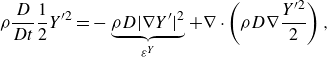 \begin{gather} \rho \frac {D}{Dt}\frac {1}{2} Y^{\prime2}= -\underbrace {\rho D|\nabla Y^{\prime}|^2}_{\mathcal {\varepsilon }^Y} + \nabla \cdot \left (\rho D \nabla \frac {Y^{\prime2}}{2}\right ), \end{gather}
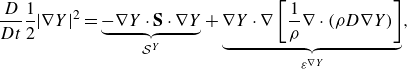 \begin{gather} \frac {D}{Dt}\frac {1}{2}|\nabla Y|^2= \underbrace {-\nabla Y \cdot \mathbf {S}\cdot \nabla Y }_{\mathcal {S}^Y} + \underbrace {\nabla Y \cdot \nabla \left [ \frac {1}{\rho } \nabla \cdot (\rho D\nabla Y)\right ]}_{\mathcal {\varepsilon }^{\nabla Y}}, \end{gather}
where $D/Dt$
is the material derivative,
$D/Dt$
is the material derivative, $Y^{\prime}=Y-Y_0$
is the fluctuating part of mass fraction and
$Y^{\prime}=Y-Y_0$
is the fluctuating part of mass fraction and $Y_0=\langle \rho Y\rangle /\langle \rho \rangle$
is the density-weighted mean concentration. Note that the equation for
$Y_0=\langle \rho Y\rangle /\langle \rho \rangle$
is the density-weighted mean concentration. Note that the equation for $Y^2$
has the same expression as (3.3) for
$Y^2$
has the same expression as (3.3) for $Y^{\prime2}$
, since
$Y^{\prime2}$
, since $Y_0$
remains constant over time due to the conservations of both mass and mass fraction. Here, we define new terms
$Y_0$
remains constant over time due to the conservations of both mass and mass fraction. Here, we define new terms $\mathcal {\varepsilon }^Y$
,
$\mathcal {\varepsilon }^Y$
, $\mathcal {S}^Y$
and
$\mathcal {S}^Y$
and $\mathcal {\varepsilon }^{\nabla Y}$
, which denote the scalar dissipation rate, the scalar element stretching rate and the scalar gradient dissipation rate, respectively.
$\mathcal {\varepsilon }^{\nabla Y}$
, which denote the scalar dissipation rate, the scalar element stretching rate and the scalar gradient dissipation rate, respectively.
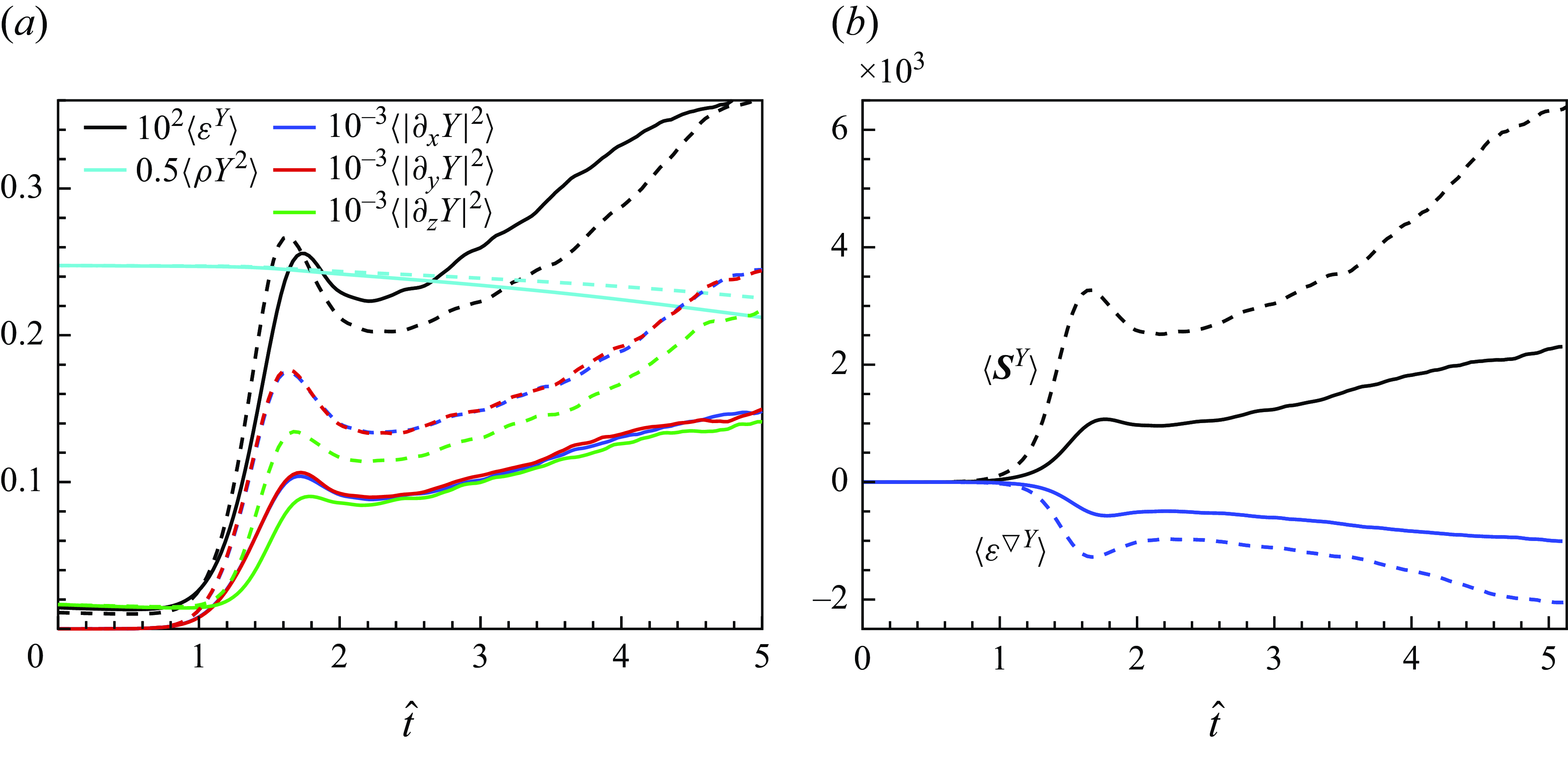
Figure 4. ( $a$
) Temporal evolution of the the mean scalar dissipation
$a$
) Temporal evolution of the the mean scalar dissipation $\langle \mathcal {\varepsilon }^Y\rangle$
, the mean scalar energy
$\langle \mathcal {\varepsilon }^Y\rangle$
, the mean scalar energy $\langle ({1}/{2})\rho Y^2 \rangle$
, as well as the three components of the mean squared mass fraction gradient. (
$\langle ({1}/{2})\rho Y^2 \rangle$
, as well as the three components of the mean squared mass fraction gradient. ( $b$
) The evolution of the mean scalar element stretching
$b$
) The evolution of the mean scalar element stretching $\langle \mathcal {S}^Y\rangle$
and the mean scalar gradient dissipation
$\langle \mathcal {S}^Y\rangle$
and the mean scalar gradient dissipation $\langle \mathcal {\varepsilon }^{\nabla Y}\rangle$
. Solid and dashed lines represent the low-At and mid-At cases, respectively.
$\langle \mathcal {\varepsilon }^{\nabla Y}\rangle$
. Solid and dashed lines represent the low-At and mid-At cases, respectively.
Equation (3.3) indicates that the spatial mean concentration variance, when scaled by density, decreases monotonically over time, with a decreasing rate of $\langle \mathcal {\varepsilon }^Y \rangle$
. In figure 4(a) we present the temporal evolution of the mean mass fraction energy,
$\langle \mathcal {\varepsilon }^Y \rangle$
. In figure 4(a) we present the temporal evolution of the mean mass fraction energy, $\langle ({1}/{2}) \rho Y^2 \rangle \equiv \langle ({1}/{2}) \rho Y^{\prime2} \rangle + ({1}/{2})\langle \rho \rangle Y_0^2$
, instead of the variance
$\langle ({1}/{2}) \rho Y^2 \rangle \equiv \langle ({1}/{2}) \rho Y^{\prime2} \rangle + ({1}/{2})\langle \rho \rangle Y_0^2$
, instead of the variance $\langle ({1}/{2}) \rho Y^{\prime2} \rangle$
, to have the same initial value between the low-At and mid-At cases. The results confirm the monotonic decay of concentration energy, and consequently, the mass fraction variance. Initially, the concentration energy is slightly less than 0.25, corresponding to fully segregated heavy and light fluids (
$\langle ({1}/{2}) \rho Y^{\prime2} \rangle$
, to have the same initial value between the low-At and mid-At cases. The results confirm the monotonic decay of concentration energy, and consequently, the mass fraction variance. Initially, the concentration energy is slightly less than 0.25, corresponding to fully segregated heavy and light fluids ( $Y=1, \rho _h=1$
on the upper half-domain so that
$Y=1, \rho _h=1$
on the upper half-domain so that $\langle ({1}/{2}) \rho Y^2 \rangle |_{t=0}=0.25$
), except in a narrow region near the fluid interface. The decay rate is slow for
$\langle ({1}/{2}) \rho Y^2 \rangle |_{t=0}=0.25$
), except in a narrow region near the fluid interface. The decay rate is slow for $\widehat {t} \lt 1.5$
, before the onset of turbulence, but after
$\widehat {t} \lt 1.5$
, before the onset of turbulence, but after $\widehat {t} \gt 2$
, during the self-similar phase, the decay rates for both cases increase, accompanied by a growing scalar gradient magnitude
$\widehat {t} \gt 2$
, during the self-similar phase, the decay rates for both cases increase, accompanied by a growing scalar gradient magnitude $\langle |\nabla Y|^2\rangle$
. Notably, the decay rate in the low-At case is faster than in the mid-At case, despite the reverse trend in the relative magnitude of the scalar gradient. This trend indicates that the density difference of the light fluids between the two cases outweighs the differences in scalar gradient magnitudes, and the constant mass diffusivity adopted in the simulations leads to a higher scalar dissipation rate
$\langle |\nabla Y|^2\rangle$
. Notably, the decay rate in the low-At case is faster than in the mid-At case, despite the reverse trend in the relative magnitude of the scalar gradient. This trend indicates that the density difference of the light fluids between the two cases outweighs the differences in scalar gradient magnitudes, and the constant mass diffusivity adopted in the simulations leads to a higher scalar dissipation rate $\mathcal {\varepsilon }^Y$
for the low-At case.
$\mathcal {\varepsilon }^Y$
for the low-At case.
The scalar gradient magnitude budget equation (3.4) indicates that $ ({1}/{2})|\nabla Y|^2$
is not a conserved invariant due to surface stretching, unlike the scalar field itself. The second term on the right-hand side,
$ ({1}/{2})|\nabla Y|^2$
is not a conserved invariant due to surface stretching, unlike the scalar field itself. The second term on the right-hand side, $\mathcal {\varepsilon }^{\nabla Y}$
, represents the dissipation of the scalar gradient, with its mean value being consistently negative and approximately equal to
$\mathcal {\varepsilon }^{\nabla Y}$
, represents the dissipation of the scalar gradient, with its mean value being consistently negative and approximately equal to $\langle -D (\nabla ^2Y)^2 \rangle$
in the
$\langle -D (\nabla ^2Y)^2 \rangle$
in the $\mathrm {At}\to 0$
limit. The blue lines in figure 4(b) confirm that the spatial mean value of
$\mathrm {At}\to 0$
limit. The blue lines in figure 4(b) confirm that the spatial mean value of $\mathcal {\varepsilon }^{\nabla Y}$
is always negative. In contrast, the first term
$\mathcal {\varepsilon }^{\nabla Y}$
is always negative. In contrast, the first term $\mathcal {S}^Y$
on the right-hand side is a primary source term in the growth of
$\mathcal {S}^Y$
on the right-hand side is a primary source term in the growth of $({1}/{2})|\nabla Y|^2$
for RT flows. To confirm that
$({1}/{2})|\nabla Y|^2$
for RT flows. To confirm that $\mathcal {S}^Y$
indeed represents the stretching of scalar elements, we express it as
$\mathcal {S}^Y$
indeed represents the stretching of scalar elements, we express it as
 \begin{align} \mathcal {S}^Y = -\nabla Y\nabla Y:\mathbf {S}= -|\nabla Y|^2\boldsymbol {n}\boldsymbol {n}:\nabla \boldsymbol {u} \approx |\nabla Y|^2 (\mathbf {I}-\boldsymbol {n}\boldsymbol {n}):\nabla \boldsymbol {u}, \end{align}
where $\boldsymbol {n}=\nabla Y/|\nabla Y|$
is the normal vector of the mass fraction isosurface pointing from the light fluid towards the heavy fluid. The incompressibility condition
$\boldsymbol {n}=\nabla Y/|\nabla Y|$
is the normal vector of the mass fraction isosurface pointing from the light fluid towards the heavy fluid. The incompressibility condition $\nabla \cdot \boldsymbol {u}=0$
approximately holds in the current compressible RT simulations, given that the initial conditions are isopycnal and the Mach numbers are low (Zhao et al. Reference Zhao, Betti and Aluie2022). The fractional rate of change of a surface element
$\nabla \cdot \boldsymbol {u}=0$
approximately holds in the current compressible RT simulations, given that the initial conditions are isopycnal and the Mach numbers are low (Zhao et al. Reference Zhao, Betti and Aluie2022). The fractional rate of change of a surface element $A$
is given by
$A$
is given by $({1}/{A})({DA}/{Dt}) \equiv (\mathbf {I} - \boldsymbol {n}\boldsymbol {n}):\nabla \boldsymbol {u}$
when surface propagation due to diffusion is negligible (Poinsot & Veynante Reference Poinsot and Veynante2005). Therefore, the right-hand side of (3.5) represents the stretching rate of the mass fraction isosurface along the tangential plane, confirming that
$({1}/{A})({DA}/{Dt}) \equiv (\mathbf {I} - \boldsymbol {n}\boldsymbol {n}):\nabla \boldsymbol {u}$
when surface propagation due to diffusion is negligible (Poinsot & Veynante Reference Poinsot and Veynante2005). Therefore, the right-hand side of (3.5) represents the stretching rate of the mass fraction isosurface along the tangential plane, confirming that $\mathcal {S}^Y$
is a weighted stretching term.
$\mathcal {S}^Y$
is a weighted stretching term.
Due to the initial stratification, the vertical scalar gradient is greater than the horizontal terms at early times, as is indicated in figure 4(a). However, when $\widehat {t} \gt 1$
, the horizontal derivatives of the mass fraction exceed the vertical component, consistent with the formation of coherent bubbles and spikes that are primarily elongated in the vertical direction. Between
$\widehat {t} \gt 1$
, the horizontal derivatives of the mass fraction exceed the vertical component, consistent with the formation of coherent bubbles and spikes that are primarily elongated in the vertical direction. Between $1 \lt \widehat {t} \lt 2$
, all components of the scalar gradient undergo a rapid increase followed by a decrease. This behaviour results from the competing effects of advection-induced surface stretching and diffusion-induced scalar gradient dissipation, as described by the right-hand side of (3.4), and corresponds with the non-monotonic evolution of the mixedness parameter
$1 \lt \widehat {t} \lt 2$
, all components of the scalar gradient undergo a rapid increase followed by a decrease. This behaviour results from the competing effects of advection-induced surface stretching and diffusion-induced scalar gradient dissipation, as described by the right-hand side of (3.4), and corresponds with the non-monotonic evolution of the mixedness parameter $\Theta$
during this period, as seen in figure 2(b). After
$\Theta$
during this period, as seen in figure 2(b). After $\widehat {t} \gt 2$
, the mean values of the mass fraction gradients increase over time, with directional anisotropy between horizontal and vertical components persisting, especially in the mid-At case with greater density contrast. These results indicate that the horizontal scalar gradient is larger than the vertical one, implying a smaller horizontal gradient length scale,
$\widehat {t} \gt 2$
, the mean values of the mass fraction gradients increase over time, with directional anisotropy between horizontal and vertical components persisting, especially in the mid-At case with greater density contrast. These results indicate that the horizontal scalar gradient is larger than the vertical one, implying a smaller horizontal gradient length scale, $L_{\varDelta , x}$
, compared with the vertical length scale,
$L_{\varDelta , x}$
, compared with the vertical length scale, $L_{\varDelta , z}$
:
$L_{\varDelta , z}$
:
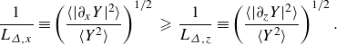 \begin{align} \frac {1}{L_{{\varDelta}, x}} \equiv \left (\frac {\langle |\partial _x Y|^2 \rangle }{\langle Y^2\rangle }\right )^{1/2} \; \geqslant \; \frac {1}{L_{\varDelta , z}} \equiv \left (\frac {\langle |\partial _z Y|^2 \rangle }{\langle Y^2\rangle }\right )^{1/2}. \end{align}
Physically, this means that at intermediate to small scales (associated with the $\nabla$
operator), the ‘eddies’ formed by the mass fraction field are elongated in the vertical direction relative to the horizontal direction (Zhao & Aluie Reference Zhao and Aluie2023).
$\nabla$
operator), the ‘eddies’ formed by the mass fraction field are elongated in the vertical direction relative to the horizontal direction (Zhao & Aluie Reference Zhao and Aluie2023).
The budget equations for scalar variance (3.3) and scalar gradient (3.4) respectively describe, at large and small scales, the annihilation and creation of the spatial variation of the transported scalar, suggesting an intrinsic connection between scalar dissipation, $\mathcal {\varepsilon }^Y$
, and scalar element stretching,
$\mathcal {\varepsilon }^Y$
, and scalar element stretching, $\mathcal {S}^Y$
. The time evolution of their spatial mean values shown in figures 4(a) and 4(b) supports this speculation, while the joint PDFs of the two quantities further validate their pointwise correlation (see figure 18 in Appendix C). The results suggest a shared underlying physical mechanism between
$\mathcal {S}^Y$
. The time evolution of their spatial mean values shown in figures 4(a) and 4(b) supports this speculation, while the joint PDFs of the two quantities further validate their pointwise correlation (see figure 18 in Appendix C). The results suggest a shared underlying physical mechanism between $\mathcal {\varepsilon }^Y$
and
$\mathcal {\varepsilon }^Y$
and $\mathcal {S}^Y$
, which is analogous to the connection between the pseudo-dissipation rate of KE,
$\mathcal {S}^Y$
, which is analogous to the connection between the pseudo-dissipation rate of KE, $\varepsilon = \nu |\boldsymbol {\omega }|^2$
, and the vortex stretching,
$\varepsilon = \nu |\boldsymbol {\omega }|^2$
, and the vortex stretching, $\boldsymbol {\omega }\cdot \mathbf {S}\cdot \boldsymbol {\omega }$
, where
$\boldsymbol {\omega }\cdot \mathbf {S}\cdot \boldsymbol {\omega }$
, where $\mathbf {S}=({1}/{2})(\nabla \boldsymbol {u}+\nabla \boldsymbol {u}^T)$
and
$\mathbf {S}=({1}/{2})(\nabla \boldsymbol {u}+\nabla \boldsymbol {u}^T)$
and $\boldsymbol {\omega }=\nabla \times \boldsymbol {u}$
are the strain rate tensor and vorticity. Vortex stretching increases local vorticity by stretching vortex tubes, leading to a higher energy dissipation rate. Similarly, in the case of mass fraction, scalar element stretching
$\boldsymbol {\omega }=\nabla \times \boldsymbol {u}$
are the strain rate tensor and vorticity. Vortex stretching increases local vorticity by stretching vortex tubes, leading to a higher energy dissipation rate. Similarly, in the case of mass fraction, scalar element stretching $\mathcal {S}^Y$
amplifies the local scalar gradient, thereby increasing the scalar dissipation rate
$\mathcal {S}^Y$
amplifies the local scalar gradient, thereby increasing the scalar dissipation rate $\mathcal {\varepsilon }^Y$
.
$\mathcal {\varepsilon }^Y$
.
To further elucidate the connection between $\mathcal {S}^Y$
and
$\mathcal {S}^Y$
and $\mathcal {\varepsilon }^Y$
, we diagonalise the strain rate tensor via eigendecomposition, yielding
$\mathcal {\varepsilon }^Y$
, we diagonalise the strain rate tensor via eigendecomposition, yielding $\mathbf {S}= \lambda _\alpha \boldsymbol {e}_\alpha \boldsymbol {e}_\alpha + \lambda _\beta \boldsymbol {e}_\beta \boldsymbol {e}_\beta + \lambda _\gamma \boldsymbol {e}_\gamma \boldsymbol {e}_\gamma$
, where
$\mathbf {S}= \lambda _\alpha \boldsymbol {e}_\alpha \boldsymbol {e}_\alpha + \lambda _\beta \boldsymbol {e}_\beta \boldsymbol {e}_\beta + \lambda _\gamma \boldsymbol {e}_\gamma \boldsymbol {e}_\gamma$
, where $\lambda _\alpha \geqslant \lambda _\beta \geqslant \lambda _\gamma$
are the eigenvalues and
$\lambda _\alpha \geqslant \lambda _\beta \geqslant \lambda _\gamma$
are the eigenvalues and $\boldsymbol {e}_\alpha , \boldsymbol {e}_\beta , \boldsymbol {e}_\gamma$
are the corresponding eigenvectors. This decomposition allows us to express the scalar element stretching as
$\boldsymbol {e}_\alpha , \boldsymbol {e}_\beta , \boldsymbol {e}_\gamma$
are the corresponding eigenvectors. This decomposition allows us to express the scalar element stretching as
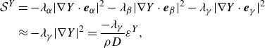 \begin{align} \begin{split} \mathcal {S}^Y &= -\lambda _\alpha |\nabla Y\cdot \boldsymbol {e}_\alpha |^2-\lambda _\beta |\nabla Y\cdot \boldsymbol {e}_\beta |^2-\lambda _\gamma |\nabla Y\cdot \boldsymbol {e}_\gamma |^2\\ &\approx -\lambda _\gamma |\nabla Y|^2 =\frac {-\lambda _\gamma }{\rho D}\mathcal {\varepsilon }^Y, \end{split} \end{align}
where the approximation holds because the scalar gradient $\nabla Y$
is primarily aligned with the eigenvector associated with the most compressive eigenvalue,
$\nabla Y$
is primarily aligned with the eigenvector associated with the most compressive eigenvalue, $\lambda _\gamma \lt 0$
, as will be verified in figure 5. In addition, the coefficient of variation (standard deviation divide by mean) of both
$\lambda _\gamma \lt 0$
, as will be verified in figure 5. In addition, the coefficient of variation (standard deviation divide by mean) of both $-\lambda _\gamma$
and
$-\lambda _\gamma$
and $\rho D$
are much smaller than that of
$\rho D$
are much smaller than that of $|\nabla Y|^2$
, indicating that the relative spatial variation of the field
$|\nabla Y|^2$
, indicating that the relative spatial variation of the field $\mathcal {\varepsilon }^Y$
is minimally influenced by the coefficient
$\mathcal {\varepsilon }^Y$
is minimally influenced by the coefficient $-\lambda _\gamma /\rho D$
. Similarly, the connection between vortex stretching and the pseudo-dissipation rate
$-\lambda _\gamma /\rho D$
. Similarly, the connection between vortex stretching and the pseudo-dissipation rate $\varepsilon =\nu |\boldsymbol {\omega }|^2$
is
$\varepsilon =\nu |\boldsymbol {\omega }|^2$
is
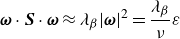 \begin{align} \boldsymbol {\omega }\cdot \boldsymbol {S} \cdot \boldsymbol {\omega } \approx \lambda _\beta |\boldsymbol {\omega }|^2 = \frac {\lambda _\beta }{\nu } \varepsilon \end{align}
since vorticity is preferentially aligned with $\boldsymbol {e}_\beta$
, and that the coefficient of variation of
$\boldsymbol {e}_\beta$
, and that the coefficient of variation of $\lambda _\beta$
is smaller than that of
$\lambda _\beta$
is smaller than that of $|\boldsymbol {\omega }|^2$
.
$|\boldsymbol {\omega }|^2$
.

Figure 5. ( $a$
) The PDF of the absolute cosine of the angle between mass fraction gradient
$a$
) The PDF of the absolute cosine of the angle between mass fraction gradient $\nabla Y$
and the three strain eigenvectors. (
$\nabla Y$
and the three strain eigenvectors. ( $b$
) The PDF of the absolute cosine of the angle between vorticity
$b$
) The PDF of the absolute cosine of the angle between vorticity $\boldsymbol {\omega }$
and the strain eigenvectors. (
$\boldsymbol {\omega }$
and the strain eigenvectors. ( $c$
) The PDF of the ratios of the largest and intermediate eigenvalues,
$c$
) The PDF of the ratios of the largest and intermediate eigenvalues, $\lambda _\alpha$
and
$\lambda _\alpha$
and $\lambda _\beta$
, to the magnitude of the most compressive eigenvalue,
$\lambda _\beta$
, to the magnitude of the most compressive eigenvalue, $|\lambda _\gamma |$
. The two vertical dashed lines correspond to the values of 0.285 and 0.710. (
$|\lambda _\gamma |$
. The two vertical dashed lines correspond to the values of 0.285 and 0.710. ( $d$
) The PDF of the cosine value between vorticity and
$d$
) The PDF of the cosine value between vorticity and $\nabla Y$
. The solid, dashed and dotted lines represent the cases of low-At, mid-At, and an incompressible passive scalar turbulence, respectively.
$\nabla Y$
. The solid, dashed and dotted lines represent the cases of low-At, mid-At, and an incompressible passive scalar turbulence, respectively.
The preferential alignment of the scalar gradient with the eigenvector corresponding to the most compressive eigenvalue is well established for passive scalars in isotropic turbulence (Batchelor Reference Batchelor1959; Ashurst et al. Reference Ashurst, Kerstein, Kerr and Gibson1987). Similarly, in RT turbulence, figure 5(a) shows that the scalar gradient $\nabla Y$
indeed aligns with the eigenvector corresponding to the most compressive eigenvalue,
$\nabla Y$
indeed aligns with the eigenvector corresponding to the most compressive eigenvalue, $\boldsymbol {e}_\gamma$
, consistent with the findings of Cabot & Zhou (Reference Cabot and Zhou2013) in incompressible variable-density RT simulations. It indicates that
$\boldsymbol {e}_\gamma$
, consistent with the findings of Cabot & Zhou (Reference Cabot and Zhou2013) in incompressible variable-density RT simulations. It indicates that $\nabla Y$
most likely aligns with
$\nabla Y$
most likely aligns with $\boldsymbol {e}_\gamma$
and is perpendicular to
$\boldsymbol {e}_\gamma$
and is perpendicular to $\boldsymbol {e}_\beta$
, while its alignment with
$\boldsymbol {e}_\beta$
, while its alignment with $\boldsymbol {e}_\alpha$
appears more random. This alignment pattern is observed in both the low-At and mid-At cases, as well as the passive scalar in isotropic turbulence, shown in solid, dashed and dotted lines, respectively. The isotropic turbulence case corresponds to a stationary forced turbulence with passive scalar using a
$\boldsymbol {e}_\alpha$
appears more random. This alignment pattern is observed in both the low-At and mid-At cases, as well as the passive scalar in isotropic turbulence, shown in solid, dashed and dotted lines, respectively. The isotropic turbulence case corresponds to a stationary forced turbulence with passive scalar using a $512^3$
grid. The alignment of vorticity with strain eigenvectors, which are shown in figure 5(b), also resembles that in incompressible isotropic turbulence, where vorticity preferentially aligns with the eigenvector
$512^3$
grid. The alignment of vorticity with strain eigenvectors, which are shown in figure 5(b), also resembles that in incompressible isotropic turbulence, where vorticity preferentially aligns with the eigenvector $\boldsymbol {e}_\beta$
corresponding to the intermediate eigenvalue. In figure 5(c) the PDFs of the eigenvalue ratios
$\boldsymbol {e}_\beta$
corresponding to the intermediate eigenvalue. In figure 5(c) the PDFs of the eigenvalue ratios $\lambda _\alpha /|\lambda _\gamma |$
and
$\lambda _\alpha /|\lambda _\gamma |$
and $\lambda _\beta /|\lambda _\gamma |$
reveal that the most probable eigenvalue triplet
$\lambda _\beta /|\lambda _\gamma |$
reveal that the most probable eigenvalue triplet $\lambda _\alpha :\lambda _\beta :\lambda _\gamma$
follows the ratio 2.84 : 1.14 : –4, close to the result of 3 : 1: –4 reported by Ashurst et al. (Reference Ashurst, Kerstein, Kerr and Gibson1987). Finally, figure 5(d) shows that the vorticity field is most likely perpendicular to the scalar gradient, with
$\lambda _\alpha :\lambda _\beta :\lambda _\gamma$
follows the ratio 2.84 : 1.14 : –4, close to the result of 3 : 1: –4 reported by Ashurst et al. (Reference Ashurst, Kerstein, Kerr and Gibson1987). Finally, figure 5(d) shows that the vorticity field is most likely perpendicular to the scalar gradient, with $\cos (\nabla Y, \boldsymbol {\omega })$
peaking at 0. This trend is applicable to the cases of low-At, mid-At and incompressible turbulence.
$\cos (\nabla Y, \boldsymbol {\omega })$
peaking at 0. This trend is applicable to the cases of low-At, mid-At and incompressible turbulence.
By combining the results from figure 5 with (3.7), we observe that in developing RT turbulence, the specific alignment between the strain field and the scalar gradient links the scalar dissipation rate $\mathcal {\varepsilon }^Y$
to the scalar element stretching rate
$\mathcal {\varepsilon }^Y$
to the scalar element stretching rate $\mathcal {S}^Y$
. This connection bridges the large-scale scalar variance
$\mathcal {S}^Y$
. This connection bridges the large-scale scalar variance ${1}/{2}\rho |Y^{\prime}|^2$
with the small-scale scalar gradient magnitude
${1}/{2}\rho |Y^{\prime}|^2$
with the small-scale scalar gradient magnitude $({1}/{2})|\nabla Y|^2$
. In the following § 4, we present scale decomposition to directly demonstrate that the transfer of scalar variance across length scales is equivalent to the scalar element stretching at a coarse-grained level.
$({1}/{2})|\nabla Y|^2$
. In the following § 4, we present scale decomposition to directly demonstrate that the transfer of scalar variance across length scales is equivalent to the scalar element stretching at a coarse-grained level.
3.3. Evolution of the direction of the scalar gradient
In addition to the scalar gradient magnitude, the evolution of the normal direction plays a crucial role in the alignment between $\nabla Y$
and the strain eigenframe, thereby influencing the magnitude of surface stretching term
$\nabla Y$
and the strain eigenframe, thereby influencing the magnitude of surface stretching term $\mathcal {S}^Y$
. The governing equation for the mass fraction normal vector,
$\mathcal {S}^Y$
. The governing equation for the mass fraction normal vector, $\boldsymbol {n}=\nabla Y/|\nabla Y|$
, is given by (Dopazo et al. Reference Dopazo, Martin, Cifuentes and Hierro2018)
$\boldsymbol {n}=\nabla Y/|\nabla Y|$
, is given by (Dopazo et al. Reference Dopazo, Martin, Cifuentes and Hierro2018)
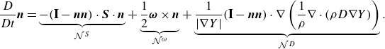 \begin{align} \frac {D}{Dt}\boldsymbol {n} = \underbrace {-(\mathbf {I}-\boldsymbol {n}\boldsymbol {n}) \cdot \boldsymbol {S} \cdot \boldsymbol {n}}_{\mathcal {N}^S} + \underbrace {\frac {1}{2}\boldsymbol {\omega }\times \boldsymbol {n}}_{\mathcal {N}^\omega } + \underbrace {\frac {1}{|\nabla Y|} (\mathbf {I} -\boldsymbol {n}\boldsymbol {n})\cdot \nabla \left (\frac {1}{\rho }\nabla \cdot (\rho D\nabla Y)\right )}_{\mathcal {N}^D}. \end{align}
Unlike the evolution of the scalar gradient magnitude described in (3.4), which depends solely on the strain rate tensor in the scalar element stretching term, the evolution of the normal vector depends on both the symmetric and anti-symmetric parts of the velocity gradient tensor. The first term on the right-hand side of (3.9), $\mathcal {N}^S$
, represents the strain-induced rotation of the normal vector on the scalar isosurface, causing it to deviate from the direction of the hydrodynamic force acting on the surface. The second term,
$\mathcal {N}^S$
, represents the strain-induced rotation of the normal vector on the scalar isosurface, causing it to deviate from the direction of the hydrodynamic force acting on the surface. The second term, $\mathcal {N}^\omega$
, accounts for the rotation of the normal vector due to vorticity, while the third term,
$\mathcal {N}^\omega$
, accounts for the rotation of the normal vector due to vorticity, while the third term, $\mathcal {N}^D$
, describes the reorientation of the normal vector related to scalar diffusion.
$\mathcal {N}^D$
, describes the reorientation of the normal vector related to scalar diffusion.
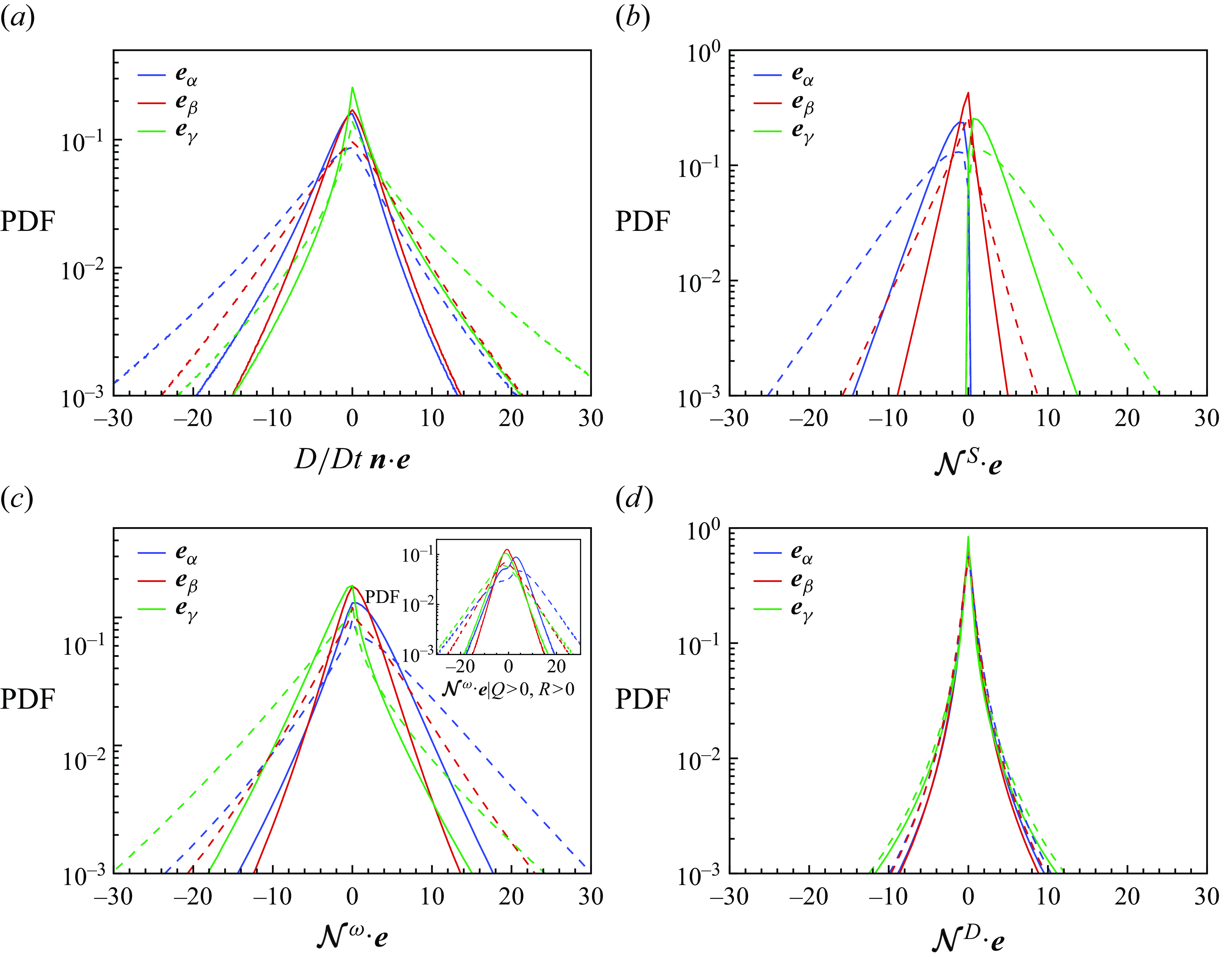
Figure 6. ( $a$
) The PDFs of the dot product between the rate of change of the scalar gradient direction and the strain eigenvectors, where the strain eigenvectors are aligned to have
$a$
) The PDFs of the dot product between the rate of change of the scalar gradient direction and the strain eigenvectors, where the strain eigenvectors are aligned to have $\cos (\boldsymbol {e}, \nabla Y)\geqslant 0$
everywhere. (b)–(d) The individual contributions from the strain term, the vorticity term and the diffusion term on the right-hand side of (3.9). Inset of panel (c) shows the PDF of
$\cos (\boldsymbol {e}, \nabla Y)\geqslant 0$
everywhere. (b)–(d) The individual contributions from the strain term, the vorticity term and the diffusion term on the right-hand side of (3.9). Inset of panel (c) shows the PDF of $\mathcal {N}^\omega \cdot \boldsymbol {e}$
conditioned on
$\mathcal {N}^\omega \cdot \boldsymbol {e}$
conditioned on $Q\gt 0, R\gt 0$
, where
$Q\gt 0, R\gt 0$
, where $Q,R$
are the second and third invariants of the velocity gradient tensor. All panels show both the low-At (solid lines) and the mid-At (dashed lines) cases at
$Q,R$
are the second and third invariants of the velocity gradient tensor. All panels show both the low-At (solid lines) and the mid-At (dashed lines) cases at $\widehat {t}=5$
.
$\widehat {t}=5$
.
Figure 6 presents the contributions to the rate of change of the scalar gradient direction, illustrating the roles of different components in the preferential alignment between $\nabla Y$
and the strain eigenvectors. The total contribution is shown in panel (a), while panels (b)–(d) show the individual contributions from the terms
$\nabla Y$
and the strain eigenvectors. The total contribution is shown in panel (a), while panels (b)–(d) show the individual contributions from the terms $\mathcal {N}^S$
,
$\mathcal {N}^S$
, $\mathcal {N}^\omega$
and
$\mathcal {N}^\omega$
and $\mathcal {N}^D$
, respectively, at
$\mathcal {N}^D$
, respectively, at $\widehat {t}=5$
(similar results are observed at other time instants). We have aligned the eigenvectors such that
$\widehat {t}=5$
(similar results are observed at other time instants). We have aligned the eigenvectors such that $\cos (\nabla Y, \boldsymbol {e})\geqslant 0$
everywhere, i.e.
$\cos (\nabla Y, \boldsymbol {e})\geqslant 0$
everywhere, i.e. $\cos (\boldsymbol {n}, \boldsymbol {e})=|\cos (\boldsymbol {n}, \boldsymbol {e})|$
. Thus, positive values of
$\cos (\boldsymbol {n}, \boldsymbol {e})=|\cos (\boldsymbol {n}, \boldsymbol {e})|$
. Thus, positive values of $({D}/{Dt})\boldsymbol {n} \cdot \boldsymbol {e}$
indicate a tendency for
$({D}/{Dt})\boldsymbol {n} \cdot \boldsymbol {e}$
indicate a tendency for $\nabla Y$
to align more strongly with the respective eigenvector, while negative values suggest a weakening of the alignment. In figure 6(a) the PDFs of
$\nabla Y$
to align more strongly with the respective eigenvector, while negative values suggest a weakening of the alignment. In figure 6(a) the PDFs of $({D}/{Dt})\boldsymbol {n} \cdot \boldsymbol {e}$
are roughly symmetric about zero, with a slight bias towards
$({D}/{Dt})\boldsymbol {n} \cdot \boldsymbol {e}$
are roughly symmetric about zero, with a slight bias towards $({D}/{Dt})\boldsymbol {n} \cdot \boldsymbol {e}_\alpha \lt 0$
and
$({D}/{Dt})\boldsymbol {n} \cdot \boldsymbol {e}_\alpha \lt 0$
and $({D}/{Dt})\boldsymbol {n} \cdot \boldsymbol {e}_\gamma \gt 0$
. This suggests that, overall, the alignment between
$({D}/{Dt})\boldsymbol {n} \cdot \boldsymbol {e}_\gamma \gt 0$
. This suggests that, overall, the alignment between $\nabla Y$
and the strain eigenvectors remains temporally stable, with a minor tendency to enhance the alignment between
$\nabla Y$
and the strain eigenvectors remains temporally stable, with a minor tendency to enhance the alignment between $\nabla Y$
and
$\nabla Y$
and $e_\gamma$
, assuming that the rate of rotation of the strain eigenbasis is a slow process (Nomura & Post Reference Nomura and Post1998) so that
$e_\gamma$
, assuming that the rate of rotation of the strain eigenbasis is a slow process (Nomura & Post Reference Nomura and Post1998) so that $({D}/{Dt})\boldsymbol {n} \cdot \boldsymbol {e} \approx ({D}/{Dt})(\boldsymbol {n} \cdot \boldsymbol {e})$
. This assumption has been verified numerically for both low- and mid-At cases at
$({D}/{Dt})\boldsymbol {n} \cdot \boldsymbol {e} \approx ({D}/{Dt})(\boldsymbol {n} \cdot \boldsymbol {e})$
. This assumption has been verified numerically for both low- and mid-At cases at $\widehat {t}=5$
(not shown). For individual contributions, panel (b) reveals that
$\widehat {t}=5$
(not shown). For individual contributions, panel (b) reveals that $\mathcal {N}^S \cdot \boldsymbol {e}_\alpha \lt 0$
and
$\mathcal {N}^S \cdot \boldsymbol {e}_\alpha \lt 0$
and $\mathcal {N}^S \cdot \boldsymbol {e}_\gamma \gt 0$
, indicating a strong reinforcement of the preferential alignment between
$\mathcal {N}^S \cdot \boldsymbol {e}_\gamma \gt 0$
, indicating a strong reinforcement of the preferential alignment between $\nabla Y$
and
$\nabla Y$
and $\boldsymbol {e}_\gamma$
. In contrast, panel (c) shows that
$\boldsymbol {e}_\gamma$
. In contrast, panel (c) shows that $\mathcal {N}^\omega$
exhibits an opposite tendency, weakening the alignment between
$\mathcal {N}^\omega$
exhibits an opposite tendency, weakening the alignment between $\nabla Y$
and
$\nabla Y$
and $\boldsymbol {e}_\gamma$
while promoting alignment with
$\boldsymbol {e}_\gamma$
while promoting alignment with $\boldsymbol {e}_\alpha$
. This effect is more pronounced in vorticity-dominated regions (with positive velocity gradient invariants
$\boldsymbol {e}_\alpha$
. This effect is more pronounced in vorticity-dominated regions (with positive velocity gradient invariants $Q$
and
$Q$
and $R$
), as highlighted in the inset of panel (c). Panel (d) shows that the diffusion term,
$R$
), as highlighted in the inset of panel (c). Panel (d) shows that the diffusion term, $\mathcal {N}^D$
, has no significant preferential contribution to any of the three eigenvectors, likely due to its passive nature. Therefore, while the strain term tends to enhance alignment between the scalar gradient and the most compressive eigenvector, the vorticity term weakens this alignment. Furthermore, figures 6(b) and 6(c) show that the PDF tails exhibit an approximate exponential decay, with fatter tails compared with the Gaussian distribution, underscoring the intermittency effect associated with RT velocity gradients.
$\mathcal {N}^D$
, has no significant preferential contribution to any of the three eigenvectors, likely due to its passive nature. Therefore, while the strain term tends to enhance alignment between the scalar gradient and the most compressive eigenvector, the vorticity term weakens this alignment. Furthermore, figures 6(b) and 6(c) show that the PDF tails exhibit an approximate exponential decay, with fatter tails compared with the Gaussian distribution, underscoring the intermittency effect associated with RT velocity gradients.
4. Transfer of scalar variance across scales
We now examine the distribution and transfer of scalar variance across different scales. Our analysis will focus on the direction (sign) of scalar variance transfer and highlight the underlying physical mechanisms driving this process.
4.1. Filtering spectra of the velocity and scalar fields
To understand the scalar transfer across different length scales, we first analyse the distribution of KE and scalar variance among different length scales and present their spectra at various times. Since the presence of walls at the top and bottom boundaries complicates the use of a straightforward Fourier transform to decompose scales along the vertical direction, we employ the filtering spectrum proposed by Sadek & Aluie (Reference Sadek and Aluie2018). This approach defines the spectra for the KE and mass fraction fields as
 \begin{align} E_{\mathrm {KE}}(k_\ell ) \equiv \frac {\rm d}{{\rm d} k_\ell } \langle \overline {\rho }_\ell |\widetilde {\boldsymbol {u}}_\ell (\boldsymbol {x})|^2\rangle /2, \qquad E_Y(k_\ell )\equiv \frac {\rm d}{{\rm d} k_\ell } \langle |\overline {Y}_\ell (\boldsymbol {x})|^2 \rangle /2, \end{align}
respectively, where $k_\ell = L_z/\ell$
is the filtering wavenumber,
$k_\ell = L_z/\ell$
is the filtering wavenumber, $\overline {f}_\ell \equiv \int G_\ell ({\boldsymbol {r}}) f(\boldsymbol {x}-{\boldsymbol {r}}) d{\boldsymbol {r}}$
is the spatial coarse graining and
$\overline {f}_\ell \equiv \int G_\ell ({\boldsymbol {r}}) f(\boldsymbol {x}-{\boldsymbol {r}}) d{\boldsymbol {r}}$
is the spatial coarse graining and $\widetilde {f}_\ell \equiv \overline {\rho f}/\overline {\rho }$
is the Favre density-weighted filtering. The filtering spectrum has been adopted in analysing 2-D and 3-D incompressible turbulence (Sadek & Aluie Reference Sadek and Aluie2018), RT turbulence (Zhao et al. Reference Zhao, Betti and Aluie2022), oceanic flows (Storer et al. Reference Storer, Buzzicotti, Khatri, Griffies and Aluie2022) and laser induced plasma dynamics (Yin et al. Reference Yin, Shang, Blackman, Collins and Aluie2023).
$\widetilde {f}_\ell \equiv \overline {\rho f}/\overline {\rho }$
is the Favre density-weighted filtering. The filtering spectrum has been adopted in analysing 2-D and 3-D incompressible turbulence (Sadek & Aluie Reference Sadek and Aluie2018), RT turbulence (Zhao et al. Reference Zhao, Betti and Aluie2022), oceanic flows (Storer et al. Reference Storer, Buzzicotti, Khatri, Griffies and Aluie2022) and laser induced plasma dynamics (Yin et al. Reference Yin, Shang, Blackman, Collins and Aluie2023).
Figure 7 shows the filtering spectra for KE and mass fraction at different time instants. In panel (a) the KE spectra increase over time across all scales, with their peaks gradually shifting toward lower $k_\ell$
, corresponding to larger scales. This behaviour, when interpreted through the Favre scale decomposition (Zhao & Aluie Reference Zhao and Aluie2018), reflects the conversion of potential energy to KE at the largest scale, followed by a cascade of KE to progressively smaller scales driven by energy fluxes in RT turbulence (Zhao et al. Reference Zhao, Betti and Aluie2022).
$k_\ell$
, corresponding to larger scales. This behaviour, when interpreted through the Favre scale decomposition (Zhao & Aluie Reference Zhao and Aluie2018), reflects the conversion of potential energy to KE at the largest scale, followed by a cascade of KE to progressively smaller scales driven by energy fluxes in RT turbulence (Zhao et al. Reference Zhao, Betti and Aluie2022).
In contrast, the mass fraction field, whose variance is an ideal invariant with no input at any scale, behaves differently compared with KE. Figure 7 (b) shows that the spectra $E_Y$
increase at small scales while decreasing at large scales. After
$E_Y$
increase at small scales while decreasing at large scales. After $\widehat {t} \geqslant 4$
, the small-scale growth of
$\widehat {t} \geqslant 4$
, the small-scale growth of $E_Y$
reaches saturation, but the decrease at large scales continues. We also include
$E_Y$
reaches saturation, but the decrease at large scales continues. We also include $E_Y$
at the initial instant (
$E_Y$
at the initial instant ( $\widehat {t} = 0$
) to illustrate the persistent trend of decreasing large-scale and increasing small-scale contents. The behaviour of
$\widehat {t} = 0$
) to illustrate the persistent trend of decreasing large-scale and increasing small-scale contents. The behaviour of $E_Y$
is closely linked to the cross-scale transfer of mass fraction variance, as we shall discuss shortly.
$E_Y$
is closely linked to the cross-scale transfer of mass fraction variance, as we shall discuss shortly.
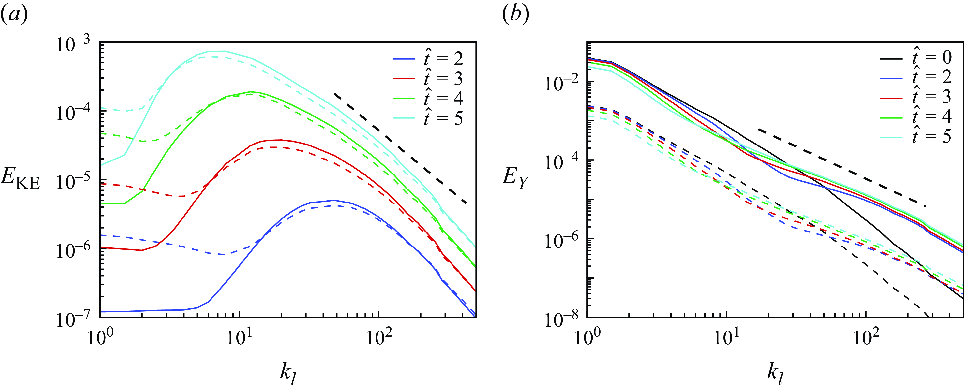
Figure 7. The filtering spectra of the ( $a$
) KE normalised by
$a$
) KE normalised by $(\rho _h-\rho _l) g L_x$
and (
$(\rho _h-\rho _l) g L_x$
and ( $b$
) mass fraction fields for the low-At (solid lines) and mid-At (dashed lines) cases at different times. The mid-At spectra of mass fraction are shifted downwards by 1 unit to distinguish from the low-At cases. The black dashed lines represent the
$b$
) mass fraction fields for the low-At (solid lines) and mid-At (dashed lines) cases at different times. The mid-At spectra of mass fraction are shifted downwards by 1 unit to distinguish from the low-At cases. The black dashed lines represent the $k_\ell ^{-5/3}$
scaling.
$k_\ell ^{-5/3}$
scaling.
4.2. Budgets of coarse-grained scalar variance and scalar gradient
Based on Favre decomposition, the budget equations for large-scale scalar variance and the scalar gradient are
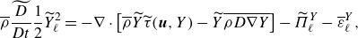 \begin{align} &\overline {\rho } \widetilde {\frac {D}{Dt}} \frac {1}{2}\widetilde {Y}_\ell ^2 = -\nabla \cdot \left [\overline {\rho } \widetilde {Y}\widetilde {\tau }(\boldsymbol {u}, Y) - \widetilde {Y} \overline {\rho D\nabla Y}\right ] - \widetilde {\Pi }_\ell ^Y - \overline {\mathcal {\varepsilon }}^Y_\ell ,\\\notag \end{align}
 \begin{align} &\overline {\rho } \widetilde {\frac {D}{Dt}}\frac {1}{2}|\nabla \widetilde {Y}_\ell |^2 =- \nabla \cdot \left [\nabla \widetilde {Y} \nabla \cdot \left (\overline {\rho }\, \widetilde {\tau }(\boldsymbol {u}, Y)\right )\right ]+\overline {\rho } \widetilde {\mathcal {S}}^Y_\ell - \widetilde {\Pi }_\ell ^{\nabla Y} - \overline {\mathcal {\varepsilon }}^{\nabla Y}_\ell . \end{align}
Here, $\widetilde {({D}/{Dt}})\equiv ({\partial }/{\partial t}) + \widetilde {\boldsymbol {u}}_\ell \cdot \nabla$
is the coarse-grained material derivative,
$\widetilde {({D}/{Dt}})\equiv ({\partial }/{\partial t}) + \widetilde {\boldsymbol {u}}_\ell \cdot \nabla$
is the coarse-grained material derivative, $\widetilde {\Pi }^Y_\ell$
and
$\widetilde {\Pi }^Y_\ell$
and $\widetilde {\Pi }_\ell ^{\nabla Y}$
are the fluxes of scalar variance and scalar gradient,
$\widetilde {\Pi }_\ell ^{\nabla Y}$
are the fluxes of scalar variance and scalar gradient, $\overline {\mathcal {\varepsilon }}^Y_\ell$
and
$\overline {\mathcal {\varepsilon }}^Y_\ell$
and $\overline {\mathcal {\varepsilon }}^{\nabla Y}_\ell$
are the coarse-grained dissipation rate of scalar and scalar gradient,
$\overline {\mathcal {\varepsilon }}^{\nabla Y}_\ell$
are the coarse-grained dissipation rate of scalar and scalar gradient, $\widetilde {\mathcal {S}}^Y_\ell$
is the filtered scalar element stretching and
$\widetilde {\mathcal {S}}^Y_\ell$
is the filtered scalar element stretching and $\widetilde {\boldsymbol \tau }(\boldsymbol {u},Y)$
is the generalised second-order moment. These terms are defined as
$\widetilde {\boldsymbol \tau }(\boldsymbol {u},Y)$
is the generalised second-order moment. These terms are defined as
 \begin{align} \begin{split} \widetilde {\Pi }^Y_\ell &= -\overline {\rho }\nabla \widetilde {Y}\cdot \widetilde {\boldsymbol \tau }(\boldsymbol {u}, Y), \;\; \widetilde {\Pi }_\ell ^{\nabla Y}=-\frac {1}{\overline {\rho }}\nabla \cdot \left (\overline {\rho }\, \widetilde {\boldsymbol \tau }(\boldsymbol {u}, Y)\right ) \nabla \cdot \left (\overline {\rho }\nabla \widetilde {Y}\right ), \; \\ \overline {\mathcal {\varepsilon }}^Y_\ell &= \nabla \widetilde {Y}\cdot \overline {\rho D \nabla Y}, \;\; \overline {\mathcal {\varepsilon }}^{\nabla Y}_\ell = -\overline {\rho } \nabla \widetilde {Y} \cdot \nabla \left (\frac {1}{\overline {\rho }}\nabla \cdot \overline {\rho D\nabla Y}\right ), \; \\ \widetilde {\mathcal {S}}^Y_\ell &= -\nabla \widetilde {Y}\cdot \nabla \widetilde {\boldsymbol {u}}\cdot \nabla \widetilde {Y}, \;\; \widetilde {\boldsymbol \tau }(\boldsymbol {u}, Y) = \widetilde {Y \boldsymbol {u}} - \widetilde {Y}\widetilde {\boldsymbol {u}}. \end{split} \end{align}
The coarse-grained scalar stretching $\widetilde {\mathcal {S}}_\ell ^Y$
approaches the fine-grained scalar stretching
$\widetilde {\mathcal {S}}_\ell ^Y$
approaches the fine-grained scalar stretching $\mathcal {S}^Y$
defined in (3.4) as
$\mathcal {S}^Y$
defined in (3.4) as $\ell$
approaches zero, i.e.
$\ell$
approaches zero, i.e. $\lim _{\ell \to 0} \widetilde {\mathcal {S}}_\ell ^Y = \mathcal {S}^Y$
.
$\lim _{\ell \to 0} \widetilde {\mathcal {S}}_\ell ^Y = \mathcal {S}^Y$
.
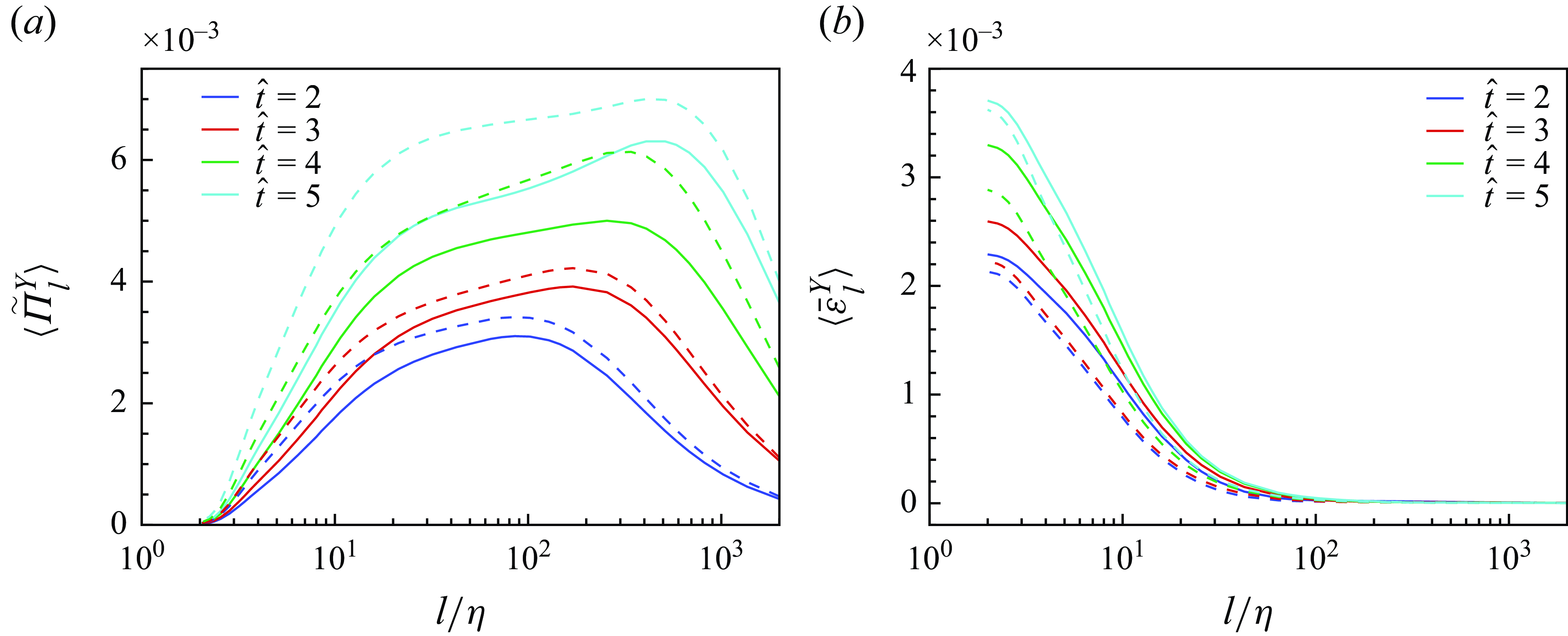
Figure 8. (a) The spatial mean values of the scalar variance flux $\widetilde {\Pi }_\ell ^Y$
with respect to the filtering width
$\widetilde {\Pi }_\ell ^Y$
with respect to the filtering width $\ell$
, normalised by the Kolmogorov scale
$\ell$
, normalised by the Kolmogorov scale $\eta$
for both the low-At (solid lines) and mid-At (dashed lines) cases over the time interval
$\eta$
for both the low-At (solid lines) and mid-At (dashed lines) cases over the time interval $\widehat {t} = 2$
--
$\widehat {t} = 2$
-- $5$
. (b) The mean coarse-grained scalar dissipation over scale,
$5$
. (b) The mean coarse-grained scalar dissipation over scale, $\overline {\mathcal {\varepsilon }}^Y_\ell$
.
$\overline {\mathcal {\varepsilon }}^Y_\ell$
.
Figure 8(a) illustrates the mean values of the scalar variance flux as functions of the filtering width $\ell$
at different time instants. All flux terms are positive on average, indicating an overall forward transfer of scalar variance from large to small scales. The transfer shows a steady increase over time (
$\ell$
at different time instants. All flux terms are positive on average, indicating an overall forward transfer of scalar variance from large to small scales. The transfer shows a steady increase over time ( $\widehat {t} = 2-5$
) as RT turbulence develops, and the length scale associated with the
$\widehat {t} = 2-5$
) as RT turbulence develops, and the length scale associated with the $\widetilde {\Pi }_\ell ^Y$
peak shifts towards larger scales. Since
$\widetilde {\Pi }_\ell ^Y$
peak shifts towards larger scales. Since $\widetilde {\Pi }^Y_\ell \equiv -\overline {\rho }\nabla \widetilde {Y}\cdot \widetilde {\boldsymbol \tau }(\boldsymbol {u},Y)$
depends on both the concentration and the velocity fields, the spectra in figure 7 demonstrate that the shift of the length scale associated with the peak
$\widetilde {\Pi }^Y_\ell \equiv -\overline {\rho }\nabla \widetilde {Y}\cdot \widetilde {\boldsymbol \tau }(\boldsymbol {u},Y)$
depends on both the concentration and the velocity fields, the spectra in figure 7 demonstrate that the shift of the length scale associated with the peak $\widetilde {\Pi }^Y_\ell$
is mainly influenced by the velocity field. Figure 8(b) shows that the dissipation of scalar variance occurs at small length scales.
$\widetilde {\Pi }^Y_\ell$
is mainly influenced by the velocity field. Figure 8(b) shows that the dissipation of scalar variance occurs at small length scales.
The influence of velocity fluctuations on the scalar variance flux can be manifested in its connection with the coarse-grained velocity gradient. We now explore the relationship of $\widetilde {\Pi }_\ell ^Y$
with the filtered velocity gradient, specifically focusing on both the strain rate and vorticity fields. The joint PDF between
$\widetilde {\Pi }_\ell ^Y$
with the filtered velocity gradient, specifically focusing on both the strain rate and vorticity fields. The joint PDF between $\widetilde {\Pi }_\ell ^Y$
and the magnitude of the filtered strain rate
$\widetilde {\Pi }_\ell ^Y$
and the magnitude of the filtered strain rate $|\overline {\mathbf {S}}_\ell |$
at
$|\overline {\mathbf {S}}_\ell |$
at $\ell = 64 \eta$
, as shown in figure 9(a), reveals a positive correlation between these two quantities. In contrast, the joint PDF between
$\ell = 64 \eta$
, as shown in figure 9(a), reveals a positive correlation between these two quantities. In contrast, the joint PDF between $\widetilde {\Pi }_\ell ^Y$
and the magnitude of the filtered vorticity
$\widetilde {\Pi }_\ell ^Y$
and the magnitude of the filtered vorticity $|\overline {\boldsymbol {\omega }}_\ell |$
in figure 9(b) shows only a very weak correlation. These trends are consistent across different filtering widths, as illustrated in the conditional mean plots in figures 9(c) and 9(d). The average
$|\overline {\boldsymbol {\omega }}_\ell |$
in figure 9(b) shows only a very weak correlation. These trends are consistent across different filtering widths, as illustrated in the conditional mean plots in figures 9(c) and 9(d). The average $\widetilde {\Pi }_\ell ^Y$
conditioned on
$\widetilde {\Pi }_\ell ^Y$
conditioned on $|\overline {\mathbf {S}}_\ell |$
is a monotonically increasing function across all cases, whereas when conditioned on
$|\overline {\mathbf {S}}_\ell |$
is a monotonically increasing function across all cases, whereas when conditioned on $|\overline {\boldsymbol \omega }_\ell |$
, the results are not monotonic and display significantly lower magnitudes. Overall, the findings in figure 9 suggest that the scalar variance flux
$|\overline {\boldsymbol \omega }_\ell |$
, the results are not monotonic and display significantly lower magnitudes. Overall, the findings in figure 9 suggest that the scalar variance flux $\widetilde {\Pi }_\ell ^Y$
is predominantly influenced by the symmetric part of the filtered velocity gradient (strain rate field) rather than the anti-symmetric part (vorticity field).
$\widetilde {\Pi }_\ell ^Y$
is predominantly influenced by the symmetric part of the filtered velocity gradient (strain rate field) rather than the anti-symmetric part (vorticity field).
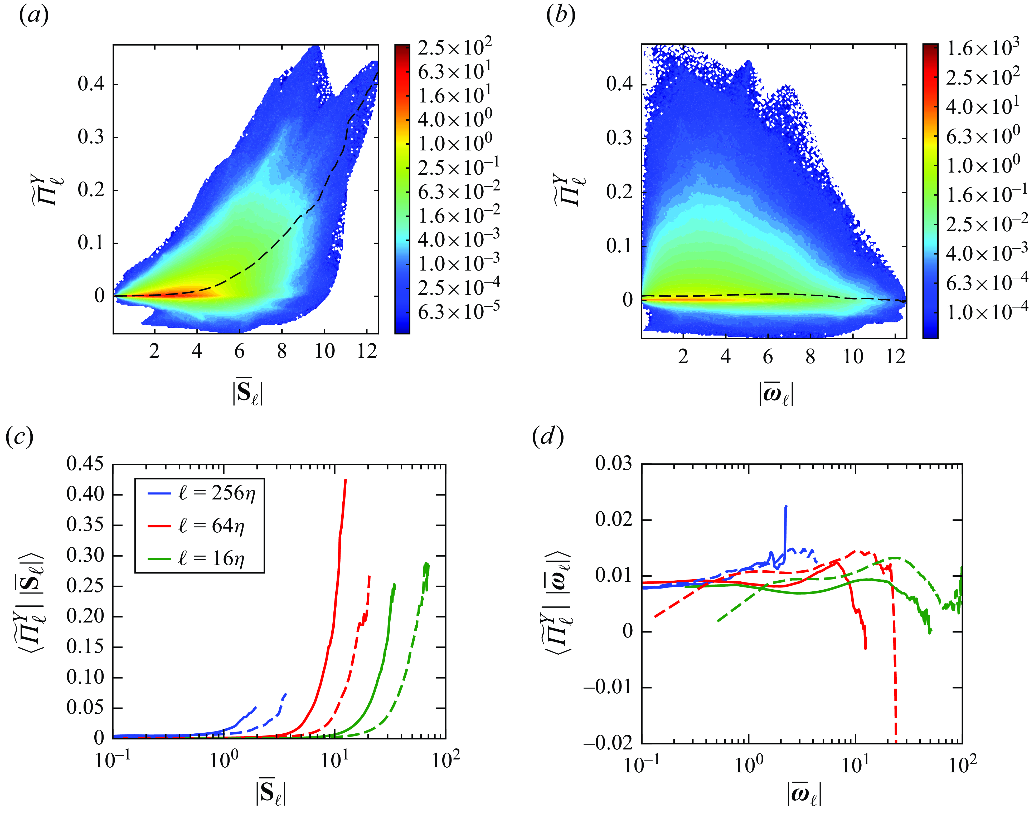
Figure 9. The correlation between scalar variance flux $\widetilde {\Pi }_\ell ^Y$
and the magnitude of the filtered strain rate and vorticity fields. Panels (a) and (b) show the joint PDF of
$\widetilde {\Pi }_\ell ^Y$
and the magnitude of the filtered strain rate and vorticity fields. Panels (a) and (b) show the joint PDF of $\widetilde {\Pi }_\ell ^Y$
with strain rate magnitude
$\widetilde {\Pi }_\ell ^Y$
with strain rate magnitude $|\overline {\boldsymbol {S}}|$
and vorticity magnitude
$|\overline {\boldsymbol {S}}|$
and vorticity magnitude $|\overline {\boldsymbol \omega }|$
, respectively, for the low-At case at filtering width
$|\overline {\boldsymbol \omega }|$
, respectively, for the low-At case at filtering width $\ell =64\eta$
and at
$\ell =64\eta$
and at $\widehat {t}=5$
. The black dashed lines are the conditional averaged scalar variance flux. Panels (c) and (d) are the conditional averaged
$\widehat {t}=5$
. The black dashed lines are the conditional averaged scalar variance flux. Panels (c) and (d) are the conditional averaged $\widetilde {\Pi }_\ell ^Y$
at three filtering widths over
$\widetilde {\Pi }_\ell ^Y$
at three filtering widths over $|\overline {\boldsymbol {S}}|$
and
$|\overline {\boldsymbol {S}}|$
and $|\overline {\boldsymbol \omega }|$
, respectively. Both the low-At (solid lines) and the mid-At (dashed lines) cases at
$|\overline {\boldsymbol \omega }|$
, respectively. Both the low-At (solid lines) and the mid-At (dashed lines) cases at $\widehat {t}=5$
are included.
$\widehat {t}=5$
are included.
This behaviour can be well explained by the nonlinear model (Borue & Orszag Reference Borue and Orszag1998; Meneveau & Katz Reference Meneveau and Katz2000b
; Lees & Aluie Reference Lees and Aluie2019). For the moment, we equate the Favre-averaged quantities with plain spatial-averaged quantities, i.e. $\widetilde {f}_\ell \approx \overline {f}_\ell$
, which incurs an error of the order
$\widetilde {f}_\ell \approx \overline {f}_\ell$
, which incurs an error of the order $O(\delta \rho /\rho )\propto O(\mathrm {At})$
(Eyink & Drivas Reference Eyink and Drivas2018). Based on this approximation, we have
$O(\delta \rho /\rho )\propto O(\mathrm {At})$
(Eyink & Drivas Reference Eyink and Drivas2018). Based on this approximation, we have $\widetilde {\boldsymbol \tau }(\boldsymbol u, Y) \approx \overline {\boldsymbol \tau }(\boldsymbol u, Y)$
. By further invoking the scale-locality property (Eyink Reference Eyink2005) for scalar fields,
$\widetilde {\boldsymbol \tau }(\boldsymbol u, Y) \approx \overline {\boldsymbol \tau }(\boldsymbol u, Y)$
. By further invoking the scale-locality property (Eyink Reference Eyink2005) for scalar fields, $\overline {\boldsymbol \tau }_\ell (\boldsymbol u, Y)\approx \overline {\boldsymbol \tau }_\ell (\overline {\boldsymbol u}_\ell , \overline {Y}_\ell )$
, and the exact identity connecting the subscale flux term for any two fields
$\overline {\boldsymbol \tau }_\ell (\boldsymbol u, Y)\approx \overline {\boldsymbol \tau }_\ell (\overline {\boldsymbol u}_\ell , \overline {Y}_\ell )$
, and the exact identity connecting the subscale flux term for any two fields $f(\boldsymbol {x}), g(\boldsymbol {x})$
and their increments (Constantin, Weinan & Titi Reference Constantin, Weinan and Titi1994)
$f(\boldsymbol {x}), g(\boldsymbol {x})$
and their increments (Constantin, Weinan & Titi Reference Constantin, Weinan and Titi1994)
 \begin{align} \overline {\tau }_\ell (f,g) = \int d^3{\boldsymbol {r}} G_\ell ({\boldsymbol {r}}) \delta f(\boldsymbol {x}; {\boldsymbol {r}}) \delta g(\boldsymbol {x};{\boldsymbol {r}}) - \int d^3{\boldsymbol {r}} G_\ell ({\boldsymbol {r}})\delta f(\boldsymbol {x};{\boldsymbol {r}})\int d^3{\boldsymbol {r}} G_\ell ({\boldsymbol {r}}) \delta g(\boldsymbol {x};{\boldsymbol {r}}), \end{align}
where $\delta f(\boldsymbol {x};{\boldsymbol {r}}) = f(\boldsymbol {x}+{\boldsymbol {r}})-f(\boldsymbol {x})$
and
$\delta f(\boldsymbol {x};{\boldsymbol {r}}) = f(\boldsymbol {x}+{\boldsymbol {r}})-f(\boldsymbol {x})$
and $\delta g(\boldsymbol {x};{\boldsymbol {r}}) = g(\boldsymbol {x}+{\boldsymbol {r}})-g(\boldsymbol {x})$
, we have
$\delta g(\boldsymbol {x};{\boldsymbol {r}}) = g(\boldsymbol {x}+{\boldsymbol {r}})-g(\boldsymbol {x})$
, we have
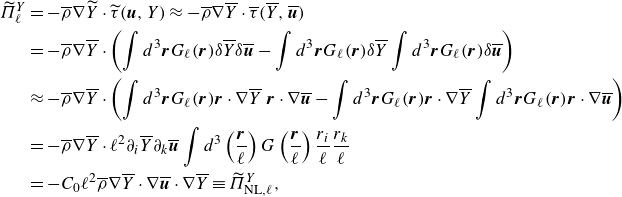 \begin{align} \begin{split} \widetilde {\Pi }_\ell ^Y &= -\overline {\rho }\nabla \widetilde {Y}\cdot \widetilde {\tau }(\boldsymbol u, Y) \approx -\overline {\rho }\nabla \overline {Y}\cdot \overline {\tau }(\overline {Y}, \overline {\boldsymbol {u}})\\ &= -\overline {\rho }\nabla \overline {Y}\cdot \left (\int d^3{\boldsymbol {r}} G_\ell ({\boldsymbol {r}}) \delta \overline {Y} \delta \overline {\boldsymbol {u}} - \int d^3{\boldsymbol {r}} G_\ell ({\boldsymbol {r}}) \delta \overline {Y} \int d^3{\boldsymbol {r}} G_\ell ({\boldsymbol {r}})\delta \overline {\boldsymbol {u}}\right ) \\ &\approx -\overline {\rho }\nabla \overline {Y}\cdot \left (\int d^3{\boldsymbol {r}} G_\ell ({\boldsymbol {r}}) {\boldsymbol {r}} \cdot \nabla \overline {Y}\ {\boldsymbol {r}}\cdot \nabla \overline {\boldsymbol {u}} - \int d^3{\boldsymbol {r}} G_\ell ({\boldsymbol {r}}) {\boldsymbol {r}} \cdot \nabla \overline {Y} \int d^3{\boldsymbol {r}} G_\ell ({\boldsymbol {r}}) {\boldsymbol {r}} \cdot \nabla \overline {\boldsymbol {u}} \right ) \\ &= -\overline {\rho }\nabla \overline {Y}\cdot \ell ^2 \partial _i \overline {Y}\partial _k \overline {\boldsymbol {u}} \int d^3\left (\frac {{\boldsymbol {r}}}{\ell }\right ) G\left (\frac {{\boldsymbol {r}}}{\ell }\right ) \frac {r_i}{\ell }\frac {r_k}{\ell } \\ &= -C_0\ell ^2 \overline {\rho } \nabla \overline {Y} \cdot \nabla \overline {\boldsymbol {u}}\cdot \nabla \overline {Y} \equiv \widetilde {\Pi }_{\mathrm {NL},\ell }^Y, \end{split} \end{align}
where between the second the third line we have adopted the Taylor expansion $\delta \overline {Y} \approx {\boldsymbol {r}} \cdot \nabla \overline {Y}, \delta \overline {\boldsymbol {u}} \approx {\boldsymbol {r}}\cdot \nabla \overline {\boldsymbol {u}}$
to further approximate the expression, and the coefficient
$\delta \overline {Y} \approx {\boldsymbol {r}} \cdot \nabla \overline {Y}, \delta \overline {\boldsymbol {u}} \approx {\boldsymbol {r}}\cdot \nabla \overline {\boldsymbol {u}}$
to further approximate the expression, and the coefficient $C_0=\int d^3{\boldsymbol {r}} G({\boldsymbol {r}})|{\boldsymbol {r}}|^2$
is the second moment of the filtering kernel and, hence, is a constant. For the Gaussian kernel adopted here in (2.6), we have
$C_0=\int d^3{\boldsymbol {r}} G({\boldsymbol {r}})|{\boldsymbol {r}}|^2$
is the second moment of the filtering kernel and, hence, is a constant. For the Gaussian kernel adopted here in (2.6), we have $C_0=1/12$
.
$C_0=1/12$
.
The nonlinear model suggests that the scalar variance flux $\widetilde {\Pi }_\ell ^Y$
across scale
$\widetilde {\Pi }_\ell ^Y$
across scale $\ell$
explicitly depends only on the strain rate tensor filtered at
$\ell$
explicitly depends only on the strain rate tensor filtered at $\ell$
, with no direct dependence on the vorticity field. This is consistent with the conditional averaged results presented in figure 9. In deriving this model, several simplifications were made that could affect its performance. We now evaluate the model by comparing its prediction with the actual data.
$\ell$
, with no direct dependence on the vorticity field. This is consistent with the conditional averaged results presented in figure 9. In deriving this model, several simplifications were made that could affect its performance. We now evaluate the model by comparing its prediction with the actual data.
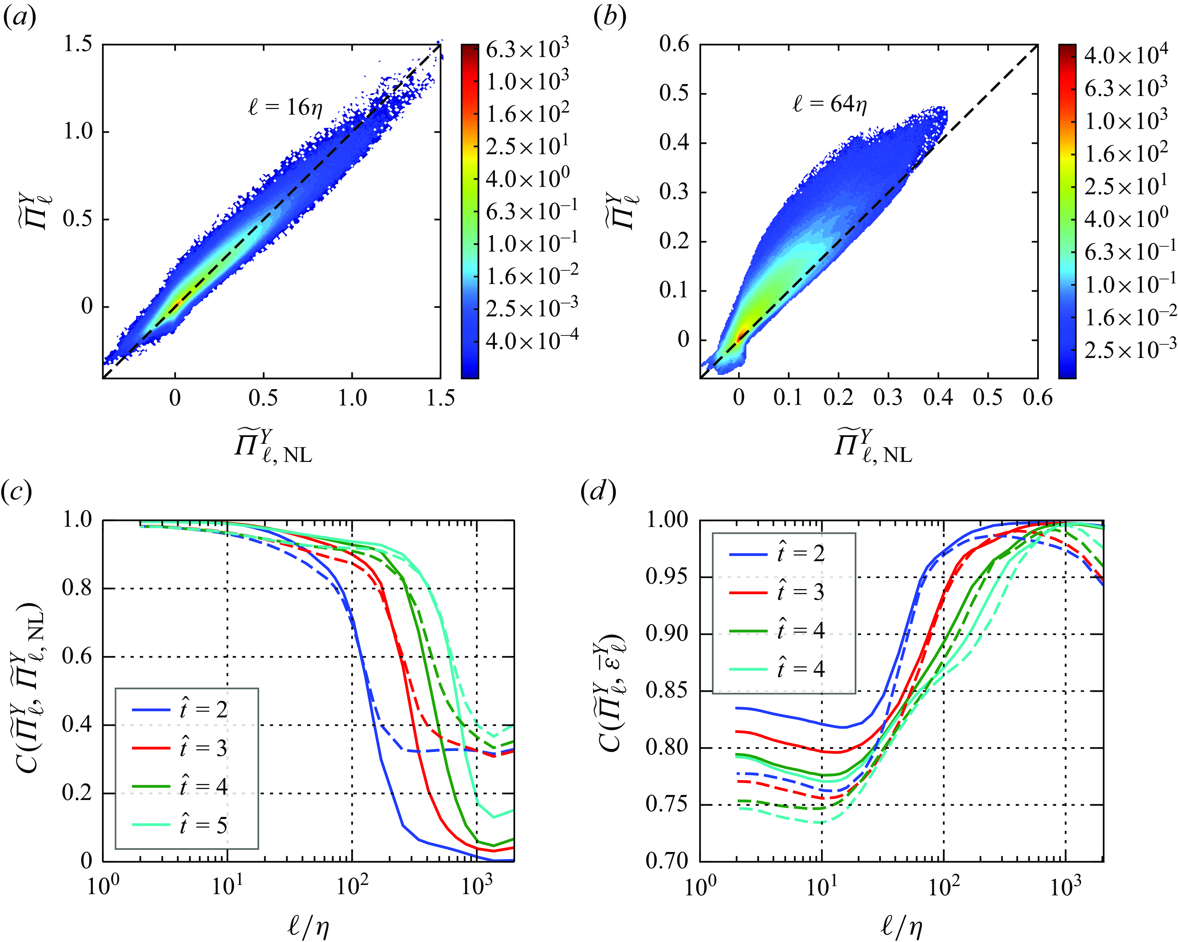
Figure 10. The joint PDF between $\widetilde {\Pi }_\ell ^Y$
and its nonlinear model
$\widetilde {\Pi }_\ell ^Y$
and its nonlinear model $\widetilde {\Pi }^Y_{\ell ,\mathrm {NL}}$
for the low-At case at
$\widetilde {\Pi }^Y_{\ell ,\mathrm {NL}}$
for the low-At case at $\widehat {t}=5$
, evaluated at two widths (
$\widehat {t}=5$
, evaluated at two widths ( $a$
)
$a$
) $\ell =16\eta$
and (
$\ell =16\eta$
and ( $b$
)
$b$
) $\ell =64\eta$
. An auxiliary diagonal dashed line is included for reference. (
$\ell =64\eta$
. An auxiliary diagonal dashed line is included for reference. ( $c$
) The correlation coefficients between
$c$
) The correlation coefficients between $\widetilde {\Pi }_\ell ^Y$
and its nonlinear model for both the low-At (solid lines) and mid-At (dashed lines) cases at
$\widetilde {\Pi }_\ell ^Y$
and its nonlinear model for both the low-At (solid lines) and mid-At (dashed lines) cases at $\widehat {t}=2-5$
. (
$\widehat {t}=2-5$
. ( $d$
) The correlation coefficients between
$d$
) The correlation coefficients between $\widetilde {\Pi }_\ell ^Y$
and
$\widetilde {\Pi }_\ell ^Y$
and $\overline {\mathcal {\varepsilon }}^Y_\ell$
.
$\overline {\mathcal {\varepsilon }}^Y_\ell$
.
Figures 10(a) and 10(b) show the joint PDF of $\widetilde {\Pi }_\ell ^Y$
and its nonlinear model
$\widetilde {\Pi }_\ell ^Y$
and its nonlinear model $\widetilde {\Pi }^Y_{\text {NL}} = -({1}/{12})\ell ^2\overline {\rho } \nabla \overline {Y} \cdot \nabla \overline {\boldsymbol {u}} \cdot \nabla \overline {Y}$
for the low-At case at
$\widetilde {\Pi }^Y_{\text {NL}} = -({1}/{12})\ell ^2\overline {\rho } \nabla \overline {Y} \cdot \nabla \overline {\boldsymbol {u}} \cdot \nabla \overline {Y}$
for the low-At case at $\widehat {t}=5$
. The joint PDFs for both small and intermediate length scales,
$\widehat {t}=5$
. The joint PDFs for both small and intermediate length scales, $\ell = 16\eta$
and
$\ell = 16\eta$
and $\ell = 64\eta$
, align closely with the diagonal line, with correlation coefficients of 0.98 and 0.94, respectively. This indicates that the nonlinear model provides a strong pointwise approximation of the actual scalar variance flux.
$\ell = 64\eta$
, align closely with the diagonal line, with correlation coefficients of 0.98 and 0.94, respectively. This indicates that the nonlinear model provides a strong pointwise approximation of the actual scalar variance flux.
Figure 10(c) further illustrates the correlation coefficient between the model and actual flux at different times ( $\widehat {t} = 2-5$
) for both the low-At and mid-At cases. The results show that the correlation improves over time as the RT turbulence develops, suggesting that the model performs better at higher Reynolds numbers where the scale-locality assumption is applicable to a wider scale range. In addition, the correlation coefficient is higher at smaller scales, where the Taylor expansion adopted in deriving the nonlinear model is more accurate. Additionally, because of the approximation that replaces Favre-filtered quantities with plain filtered quantities,
$\widehat {t} = 2-5$
) for both the low-At and mid-At cases. The results show that the correlation improves over time as the RT turbulence develops, suggesting that the model performs better at higher Reynolds numbers where the scale-locality assumption is applicable to a wider scale range. In addition, the correlation coefficient is higher at smaller scales, where the Taylor expansion adopted in deriving the nonlinear model is more accurate. Additionally, because of the approximation that replaces Favre-filtered quantities with plain filtered quantities, $\widetilde {f}(\boldsymbol {x}) \to \overline {f}(\boldsymbol {x})$
, the low-At case shows slightly better correlation than the mid-At case at small to intermediate scales, due to the smaller error of the order
$\widetilde {f}(\boldsymbol {x}) \to \overline {f}(\boldsymbol {x})$
, the low-At case shows slightly better correlation than the mid-At case at small to intermediate scales, due to the smaller error of the order $O(\mathrm {At})$
. Interestingly, the correlation coefficients for the mid-At case at the largest filtering widths are slightly better than those in the low-At case, despite the overall relatively weak correlation. This trend is likely due to the higher Reynolds number in the mid-At case than the low-At case, as indicated in table 1, leading to a slightly better performance of the model. In addition, the time evolution of the mean values of
$O(\mathrm {At})$
. Interestingly, the correlation coefficients for the mid-At case at the largest filtering widths are slightly better than those in the low-At case, despite the overall relatively weak correlation. This trend is likely due to the higher Reynolds number in the mid-At case than the low-At case, as indicated in table 1, leading to a slightly better performance of the model. In addition, the time evolution of the mean values of $\widetilde {\Pi }_\ell ^Y$
and
$\widetilde {\Pi }_\ell ^Y$
and $\widetilde {\Pi }^Y_{\text {NL}}$
, along with their correlation coefficients, are illustrated in Appendix D. These results again demonstrate the good approximation of the nonlinear model within the self-similar regime of RT turbulence.
$\widetilde {\Pi }^Y_{\text {NL}}$
, along with their correlation coefficients, are illustrated in Appendix D. These results again demonstrate the good approximation of the nonlinear model within the self-similar regime of RT turbulence.
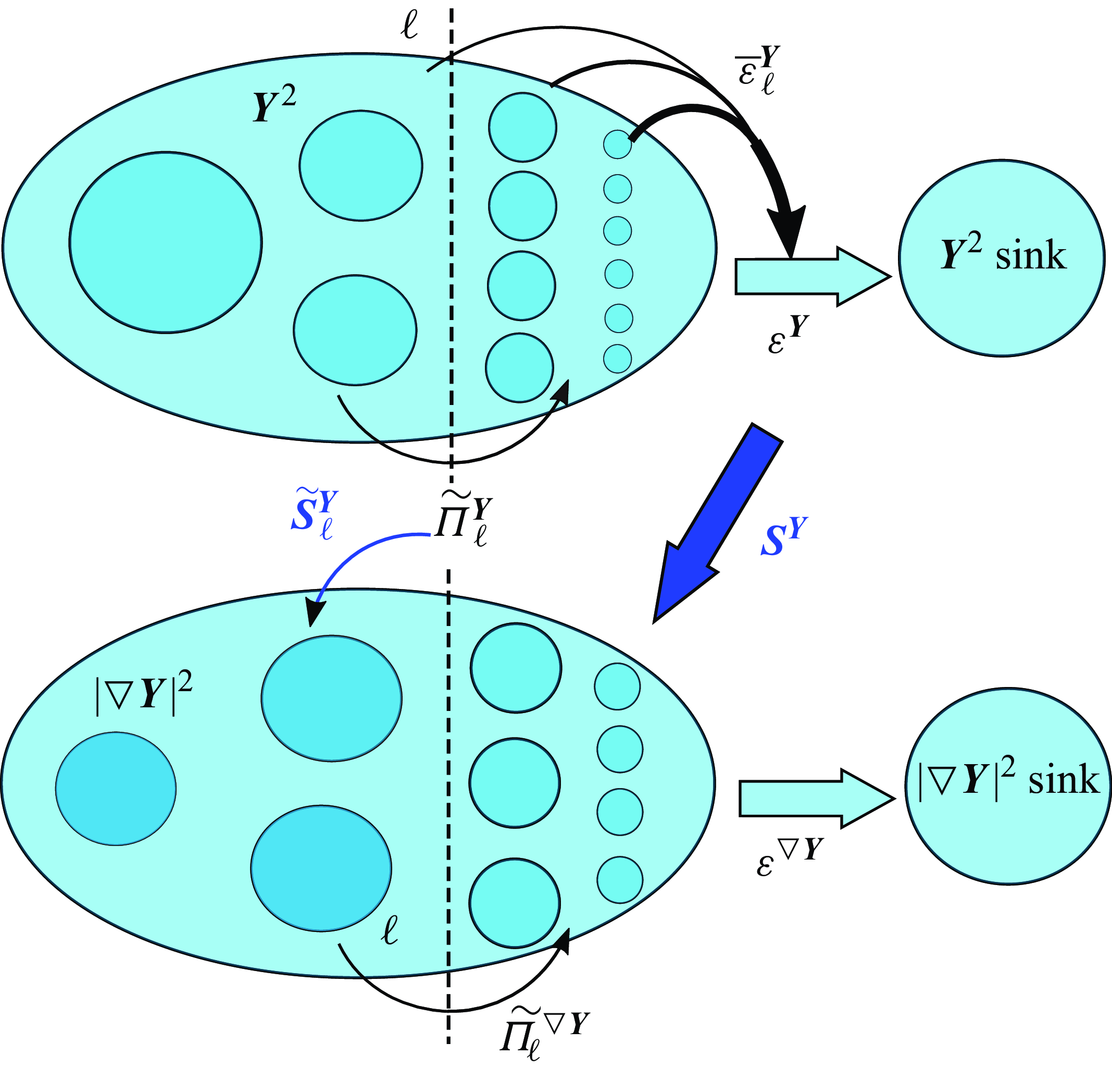
Figure 11. Schematic of the pathway of scalar variance and its gradient transfer across scales.
The nonlinear model $\widetilde {\Pi }^Y_{\ell ,\mathrm {NL}}$
bears a strong resemblance to the filtered scalar stretching term
$\widetilde {\Pi }^Y_{\ell ,\mathrm {NL}}$
bears a strong resemblance to the filtered scalar stretching term $\widetilde {\mathcal {S}}^Y_\ell = -\partial _i \widetilde {Y}\partial _j \widetilde {Y}\partial _i \widetilde {u}_j \approx -\partial _i \overline {Y} \partial _j\overline {Y}\partial _i \overline {u}_j = \widetilde {\Pi }_{\ell ,\mathrm {NL}}^Y/(C_0\ell ^2 \overline {\rho })$
. This similarity indicates a shared physical mechanism underlying both the scalar variance flux, a sink term for large-scale scalar variance in (4.2), and the filtered scalar stretching, which acts as a source term in the coarse-grained scalar gradient equation (4.3). Given that the preferential alignment between the scalar gradient and the strain eigenbasis also holds for coarse-grained fields (see figure 13
a), the estimation in (3.7) that connects the fine-grained stretching term and the scalar dissipation rate is valid for the filtered results as well, i.e.
$\widetilde {\mathcal {S}}^Y_\ell = -\partial _i \widetilde {Y}\partial _j \widetilde {Y}\partial _i \widetilde {u}_j \approx -\partial _i \overline {Y} \partial _j\overline {Y}\partial _i \overline {u}_j = \widetilde {\Pi }_{\ell ,\mathrm {NL}}^Y/(C_0\ell ^2 \overline {\rho })$
. This similarity indicates a shared physical mechanism underlying both the scalar variance flux, a sink term for large-scale scalar variance in (4.2), and the filtered scalar stretching, which acts as a source term in the coarse-grained scalar gradient equation (4.3). Given that the preferential alignment between the scalar gradient and the strain eigenbasis also holds for coarse-grained fields (see figure 13
a), the estimation in (3.7) that connects the fine-grained stretching term and the scalar dissipation rate is valid for the filtered results as well, i.e.
 \begin{align} \widetilde {\Pi }^Y_\ell \approx \widetilde {\Pi }^Y_{\ell , \mathrm {NL}} \propto \widetilde {\mathcal {S}}^Y_\ell \approx -\overline {\lambda }_\gamma |\nabla \overline {Y}_\ell |^2 \approx \frac {-\overline {\lambda }_\gamma }{\overline {\rho }_\ell D}\overline {\mathcal {\varepsilon }}_\ell ^Y \quad \mathrm {given }\; \nabla \overline {Y}_\ell \parallel \boldsymbol {e}_{\gamma }, \end{align}
where $\overline {\lambda }_\gamma$
is the eigenvalue corresponding to the most compressive eigenvector of the filtered strain field. The correlation between
$\overline {\lambda }_\gamma$
is the eigenvalue corresponding to the most compressive eigenvector of the filtered strain field. The correlation between $\widetilde {\Pi }^Y_\ell$
and the large-scale scalar dissipation
$\widetilde {\Pi }^Y_\ell$
and the large-scale scalar dissipation $\overline {\mathcal {\varepsilon }}_\ell ^Y$
is illustrated in figure 10(d), where the correlation coefficients are above 0.7 at small scales, confirming the validity of (4.7). This relation reflects a form of turbulent eddy diffusivity commonly adopted in RANS or LES. Note that in figure 10(d) the unexpectedly high correlation between
$\overline {\mathcal {\varepsilon }}_\ell ^Y$
is illustrated in figure 10(d), where the correlation coefficients are above 0.7 at small scales, confirming the validity of (4.7). This relation reflects a form of turbulent eddy diffusivity commonly adopted in RANS or LES. Note that in figure 10(d) the unexpectedly high correlation between $\widetilde {\Pi }^Y_\ell$
and
$\widetilde {\Pi }^Y_\ell$
and $\overline {\mathcal {\varepsilon }}_\ell ^Y$
at large filtering scales arises from the contribution of long-wavelength modes in RT turbulence, generated by the bubble merger process. The vertical velocity and mass fraction field of these modes combine to produce a second-order moment
$\overline {\mathcal {\varepsilon }}_\ell ^Y$
at large filtering scales arises from the contribution of long-wavelength modes in RT turbulence, generated by the bubble merger process. The vertical velocity and mass fraction field of these modes combine to produce a second-order moment $\widetilde {\tau }_\ell (\boldsymbol {u}, \boldsymbol {Y})$
that resembles the filtered mass fraction gradient, resulting in a strong correlation
$\widetilde {\tau }_\ell (\boldsymbol {u}, \boldsymbol {Y})$
that resembles the filtered mass fraction gradient, resulting in a strong correlation $C(\widetilde {\Pi }^Y_\ell , \overline {\mathcal {\varepsilon }}_\ell ^Y) \approx 1$
.
$C(\widetilde {\Pi }^Y_\ell , \overline {\mathcal {\varepsilon }}_\ell ^Y) \approx 1$
.
The pathways of scalar variance and scalar gradient transfer across scales and the underlying physical mechanism is depicted in figure 11. At intermediate to large scales ( $\gtrapprox \ell$
), turbulent stirring by straining motion disperses the bulk scalar field at large scale into sheet structures associated with smaller length scales, thus transferring scalar variance from large to small scales. Therefore, the strain-induced surface stretching
$\gtrapprox \ell$
), turbulent stirring by straining motion disperses the bulk scalar field at large scale into sheet structures associated with smaller length scales, thus transferring scalar variance from large to small scales. Therefore, the strain-induced surface stretching $\widetilde {\mathcal {S}}_\ell ^Y$
is closely related to the transfer term
$\widetilde {\mathcal {S}}_\ell ^Y$
is closely related to the transfer term $\widetilde {\Pi }_\ell ^Y$
. On the other hand, the surface stretching
$\widetilde {\Pi }_\ell ^Y$
. On the other hand, the surface stretching $\widetilde {\mathcal {S}}_\ell ^Y$
acts on the tangential plane of scalar isosurfaces, accompanied by a compression in the normal direction, which brings adjacent isoscalar elements closer together and increases the coarse-grained scalar gradient
$\widetilde {\mathcal {S}}_\ell ^Y$
acts on the tangential plane of scalar isosurfaces, accompanied by a compression in the normal direction, which brings adjacent isoscalar elements closer together and increases the coarse-grained scalar gradient $\nabla \overline {Y}_\ell$
. This effect further facilitates the dissipation rate
$\nabla \overline {Y}_\ell$
. This effect further facilitates the dissipation rate $\overline {\mathcal {\varepsilon }}^Y_\ell$
associated with the filtered concentration field. The close proximity among
$\overline {\mathcal {\varepsilon }}^Y_\ell$
associated with the filtered concentration field. The close proximity among $\widetilde {\Pi }_\ell ^Y \sim \widetilde {\mathcal {S}}_\ell ^Y \sim \overline {\mathcal {\varepsilon }}^Y_\ell$
is thus established. Additionally, since
$\widetilde {\Pi }_\ell ^Y \sim \widetilde {\mathcal {S}}_\ell ^Y \sim \overline {\mathcal {\varepsilon }}^Y_\ell$
is thus established. Additionally, since $\lim _{\ell \to 0} \widetilde {\mathcal {S}}_\ell ^Y = \mathcal {S}^Y$
and
$\lim _{\ell \to 0} \widetilde {\mathcal {S}}_\ell ^Y = \mathcal {S}^Y$
and $\lim _{\ell \to 0}\overline {\mathcal {\varepsilon }}^Y_\ell = \mathcal {\varepsilon }^Y$
, the fine-grained quantities
$\lim _{\ell \to 0}\overline {\mathcal {\varepsilon }}^Y_\ell = \mathcal {\varepsilon }^Y$
, the fine-grained quantities $\mathcal {S}^Y$
and
$\mathcal {S}^Y$
and $\mathcal {\varepsilon }^Y$
also bear similarities, as shown earlier,
$\mathcal {\varepsilon }^Y$
also bear similarities, as shown earlier,
4.3. Backscatter of the scalar variance flux
As observed in figures 9(a) and 10(a,b), while the mean value of $\widetilde {\Pi }_\ell ^Y$
is positive, causing a globally forward transfer of the scalar variance flux from large to small scales, locally negative values of
$\widetilde {\Pi }_\ell ^Y$
is positive, causing a globally forward transfer of the scalar variance flux from large to small scales, locally negative values of $\widetilde {\Pi }_\ell ^Y$
do exist, particularly at small filtering widths
$\widetilde {\Pi }_\ell ^Y$
do exist, particularly at small filtering widths $\ell$
, representing a backward transfer from small to large scales. Figure 12(a) illustrates the mean values of the positive and negative components of
$\ell$
, representing a backward transfer from small to large scales. Figure 12(a) illustrates the mean values of the positive and negative components of $\widetilde {\Pi }_\ell ^Y$
, showing that their magnitudes increase over time for both the low-At and mid-At cases. The positive component,
$\widetilde {\Pi }_\ell ^Y$
, showing that their magnitudes increase over time for both the low-At and mid-At cases. The positive component, $\widetilde {\Pi }^Y_{\ell ,+}$
, is significant across almost all scale ranges, whereas the negative component,
$\widetilde {\Pi }^Y_{\ell ,+}$
, is significant across almost all scale ranges, whereas the negative component, $\widetilde {\Pi }^Y_{\ell ,-}$
, is only prominent at relatively small length scales (
$\widetilde {\Pi }^Y_{\ell ,-}$
, is only prominent at relatively small length scales ( $\ell \lt 160\eta$
) and peaks around
$\ell \lt 160\eta$
) and peaks around $16 \eta$
. These results indicate that inverse scalar variance transfer predominantly occurs at small scales. Although the mean value of the negative subset of
$16 \eta$
. These results indicate that inverse scalar variance transfer predominantly occurs at small scales. Although the mean value of the negative subset of $\widetilde {\Pi }_\ell ^Y$
is small compared with the positive subset, the proportion of the number of
$\widetilde {\Pi }_\ell ^Y$
is small compared with the positive subset, the proportion of the number of $\widetilde {\Pi }^Y_{\ell ,-}$
samples depicted in figure 12(a) shows that the negative region could exceed 40 % at intermediate to small scales. This suggests that scalar variance backscatter has a widespread influence.
$\widetilde {\Pi }^Y_{\ell ,-}$
samples depicted in figure 12(a) shows that the negative region could exceed 40 % at intermediate to small scales. This suggests that scalar variance backscatter has a widespread influence.
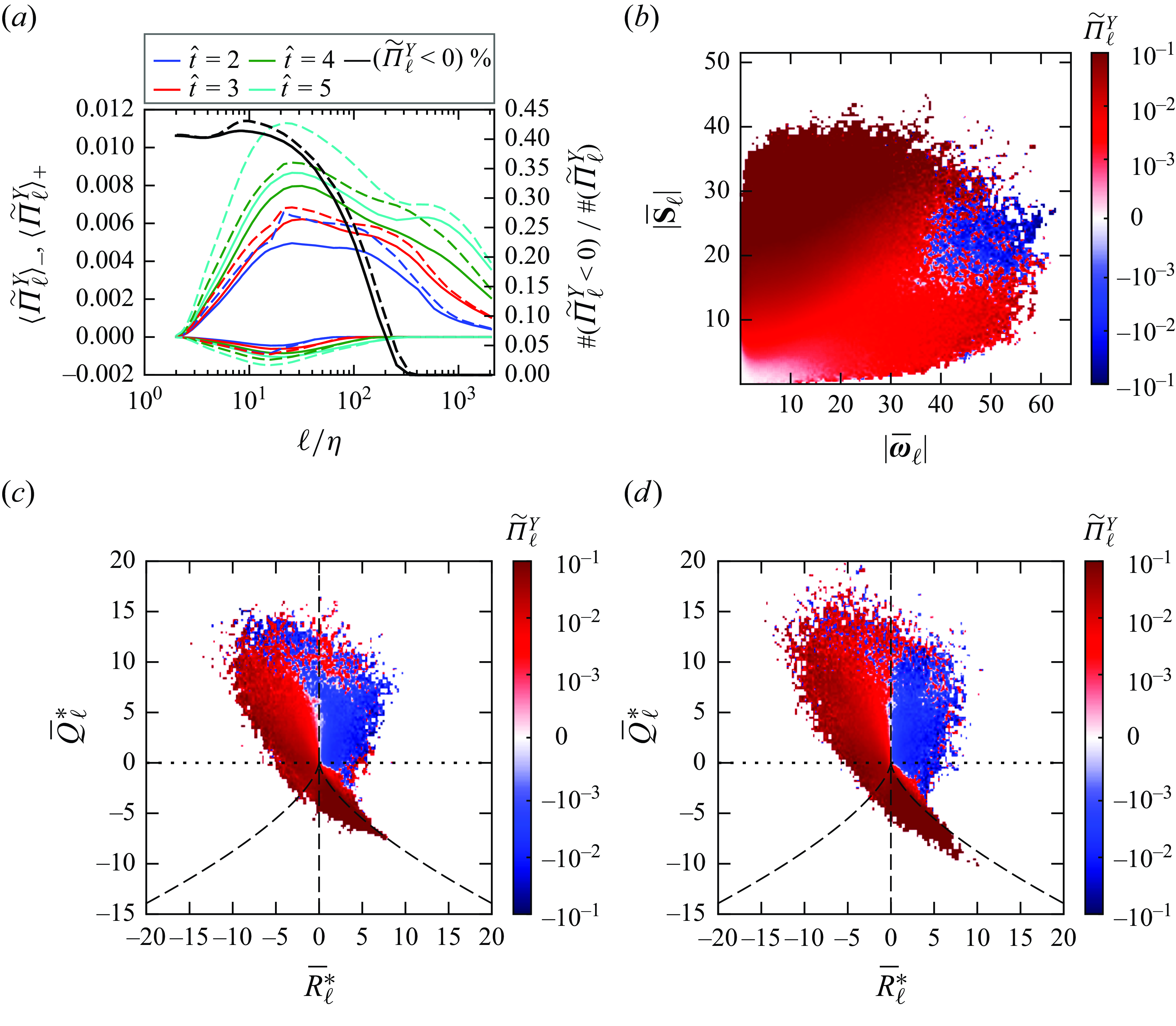
Figure 12. ( $a$
) The mean positive and negative components of the scalar variance flux, with the subscripts
$a$
) The mean positive and negative components of the scalar variance flux, with the subscripts $\langle \cdot \rangle _+$
and
$\langle \cdot \rangle _+$
and $\langle \cdot \rangle _-$
indicating averages over its positive and negative subsets, respectively. The black lines represent the proportion of the negative volume of
$\langle \cdot \rangle _-$
indicating averages over its positive and negative subsets, respectively. The black lines represent the proportion of the negative volume of $\widetilde {\Pi }_\ell ^Y$
within the domain at
$\widetilde {\Pi }_\ell ^Y$
within the domain at $\widehat {t}=5$
. (
$\widehat {t}=5$
. ( $b$
) The conditional mean value
$b$
) The conditional mean value $\langle \widetilde {\Pi }_\ell ^Y | |\overline {\mathbf {S}}_\ell |, |\overline {\boldsymbol {\omega }}_\ell | \rangle$
on the joint PDF of filtered strain and vorticity magnitudes of the low-At case at
$\langle \widetilde {\Pi }_\ell ^Y | |\overline {\mathbf {S}}_\ell |, |\overline {\boldsymbol {\omega }}_\ell | \rangle$
on the joint PDF of filtered strain and vorticity magnitudes of the low-At case at $\widehat {t}=5$
, with a filtering width
$\widehat {t}=5$
, with a filtering width $\ell =16 \eta$
. (
$\ell =16 \eta$
. ( $c, d$
) The conditional mean
$c, d$
) The conditional mean $\langle \widetilde {\Pi }_\ell ^Y | \overline {Q}^*_\ell , \overline {R}^*_\ell \rangle$
for the low-At and mid-At cases at
$\langle \widetilde {\Pi }_\ell ^Y | \overline {Q}^*_\ell , \overline {R}^*_\ell \rangle$
for the low-At and mid-At cases at $\widehat {t}=5$
with the filtering width
$\widehat {t}=5$
with the filtering width $\ell =16\eta$
. The second and third velocity gradient invariants
$\ell =16\eta$
. The second and third velocity gradient invariants $\overline {Q}_\ell$
and
$\overline {Q}_\ell$
and $\overline {R}_\ell$
are normalised by
$\overline {R}_\ell$
are normalised by $\langle |\overline {\boldsymbol {\omega }}_\ell |^2\rangle$
and
$\langle |\overline {\boldsymbol {\omega }}_\ell |^2\rangle$
and $\langle |\overline {\boldsymbol {\omega }}_\ell |^2\rangle ^{3/2}$
, respectively.
$\langle |\overline {\boldsymbol {\omega }}_\ell |^2\rangle ^{3/2}$
, respectively.
To gain insight into the spatial distribution and topology of the backscatter of scalar variance flux, we obtain the mean value of $\widetilde {\Pi }_\ell ^Y$
conditional on the
$\widetilde {\Pi }_\ell ^Y$
conditional on the $|\overline {\mathbf {S}}_\ell |$
−
$|\overline {\mathbf {S}}_\ell |$
− $|\overline {\boldsymbol {\omega }}_\ell |$
space and the
$|\overline {\boldsymbol {\omega }}_\ell |$
space and the $\overline {Q}_\ell$
−
$\overline {Q}_\ell$
− $\overline {R}_\ell$
space in figure 12(b)–(d), where
$\overline {R}_\ell$
space in figure 12(b)–(d), where $\overline {Q}_\ell \equiv -({1}/{2})\partial _k \overline {u}_i\partial _i \overline {u}_k$
and
$\overline {Q}_\ell \equiv -({1}/{2})\partial _k \overline {u}_i\partial _i \overline {u}_k$
and $\overline {R}_\ell \equiv -({1}/{3})\partial _j \overline {u}_i\partial _k\overline {u}_j\partial _i\overline {u}_k$
are the second and third invariants of the filtered velocity gradients. In the
$\overline {R}_\ell \equiv -({1}/{3})\partial _j \overline {u}_i\partial _k\overline {u}_j\partial _i\overline {u}_k$
are the second and third invariants of the filtered velocity gradients. In the $|\overline {\mathbf {S}}_\ell |$
−
$|\overline {\mathbf {S}}_\ell |$
− $|\overline {\boldsymbol {\omega }}_\ell |$
space, the negative
$|\overline {\boldsymbol {\omega }}_\ell |$
space, the negative $\widetilde {\Pi }_\ell ^Y$
occurs at regions with high-vorticity magnitude and low to intermediate strain magnitude, implying that vorticity plays an active role in the scalar variance backscatter. Figure 12(b) shows the result for the low-At case, with similar results observed for the mid-At case (not shown). In the
$\widetilde {\Pi }_\ell ^Y$
occurs at regions with high-vorticity magnitude and low to intermediate strain magnitude, implying that vorticity plays an active role in the scalar variance backscatter. Figure 12(b) shows the result for the low-At case, with similar results observed for the mid-At case (not shown). In the $\overline {Q}_\ell$
−
$\overline {Q}_\ell$
− $\overline {R}_\ell$
space shown in figures 12(c) and 12(d), the conditional joint PDFs clearly show that, for both the low-At and mid-At cases, negative mean values of
$\overline {R}_\ell$
space shown in figures 12(c) and 12(d), the conditional joint PDFs clearly show that, for both the low-At and mid-At cases, negative mean values of $\widetilde {\Pi }_\ell ^Y$
primarily occur in the first quadrant of the
$\widetilde {\Pi }_\ell ^Y$
primarily occur in the first quadrant of the $\overline {Q}_\ell{-}\overline {R}_\ell$
plane, where
$\overline {Q}_\ell{-}\overline {R}_\ell$
plane, where $\overline {Q}_\ell \gt 0$
and
$\overline {Q}_\ell \gt 0$
and $\overline {R}_\ell \gt 0$
. This region, located above the dashed curve on the right (the Vieillefosse tail,
$\overline {R}_\ell \gt 0$
. This region, located above the dashed curve on the right (the Vieillefosse tail, ${27}/{4} \overline {R}_\ell ^2 + \overline {Q}_\ell ^3 = 0$
), corresponds to the local flow pattern of vortex compression (Meneveau Reference Meneveau2011), and that local vorticity strength dominates over strain (
${27}/{4} \overline {R}_\ell ^2 + \overline {Q}_\ell ^3 = 0$
), corresponds to the local flow pattern of vortex compression (Meneveau Reference Meneveau2011), and that local vorticity strength dominates over strain ( $\overline {Q}_\ell \gt 0$
). Thus, the vorticity vector influences the backscatter region with
$\overline {Q}_\ell \gt 0$
). Thus, the vorticity vector influences the backscatter region with $\widetilde {\Pi }_\ell ^Y\lt 0$
, although its effect on the overall flux term
$\widetilde {\Pi }_\ell ^Y\lt 0$
, although its effect on the overall flux term $\widetilde {\Pi }_\ell$
is diminished, as indicated in the conditional mean of figure 9(d).
$\widetilde {\Pi }_\ell$
is diminished, as indicated in the conditional mean of figure 9(d).
The negative scalar variance transfer is due to a modified preferential alignment between the filtered scalar gradient and the filtered strain rate eigenvectors. Due to the proximity between scalar variance flux and surface stretching, we have
 \begin{align} \begin{split} \widetilde {\Pi }_\ell ^Y \propto \widetilde {\mathcal {S}}^Y &=-\partial _i \widetilde {Y}\partial _j \widetilde {Y}\widetilde {\mathrm S}_{ij} \approx -\partial _i \overline {Y}\partial _j \overline {Y}\overline {\mathrm S}_{ij}\\ &= -|\nabla \overline {Y}|^2\left (\overline {\lambda }_\alpha \cos ^2(\nabla \overline {Y}, \boldsymbol {e}_{\alpha })+ \overline {\lambda }_\beta \cos ^2(\nabla \overline {Y}, \boldsymbol {e}_{\beta })+ \overline {\lambda }_\gamma \cos ^2(\nabla \overline {Y}, \boldsymbol {e}_{\gamma })\right ), \end{split} \end{align}
where $\overline {\lambda }_\alpha , \overline {\lambda }_\beta , \overline {\lambda }_\gamma$
and
$\overline {\lambda }_\alpha , \overline {\lambda }_\beta , \overline {\lambda }_\gamma$
and $\boldsymbol {e}_{\alpha }, \boldsymbol {e}_{\beta }, \boldsymbol {e}_{\gamma }$
correspond to the eigenvalues and eigenvectors of the filtered strain rate tensor
$\boldsymbol {e}_{\alpha }, \boldsymbol {e}_{\beta }, \boldsymbol {e}_{\gamma }$
correspond to the eigenvalues and eigenvectors of the filtered strain rate tensor $\overline {\boldsymbol {S}}$
, with
$\overline {\boldsymbol {S}}$
, with $\overline {\lambda }_\alpha \gt 0$
and
$\overline {\lambda }_\alpha \gt 0$
and $\overline {\lambda }_\gamma \lt 0$
. Thus, if
$\overline {\lambda }_\gamma \lt 0$
. Thus, if $\nabla \overline {Y}$
predominantly aligns with the most compressive eigenvector
$\nabla \overline {Y}$
predominantly aligns with the most compressive eigenvector $\boldsymbol {e}_{\gamma }$
then
$\boldsymbol {e}_{\gamma }$
then $\widetilde {\Pi }_\ell ^Y \propto -\overline {\lambda }_\gamma |\nabla \overline {Y}|^2 \cos (\nabla \overline {Y}, \boldsymbol {e}_{\gamma })^2 \gt 0$
. On the other hand, if
$\widetilde {\Pi }_\ell ^Y \propto -\overline {\lambda }_\gamma |\nabla \overline {Y}|^2 \cos (\nabla \overline {Y}, \boldsymbol {e}_{\gamma })^2 \gt 0$
. On the other hand, if $\nabla \overline {Y}$
predominantly aligns with the most expansive eigenvector
$\nabla \overline {Y}$
predominantly aligns with the most expansive eigenvector $\boldsymbol {e}_{\alpha }$
then
$\boldsymbol {e}_{\alpha }$
then $\widetilde {\Pi }_\ell ^Y \propto -\overline {\lambda }_\alpha |\nabla \overline {Y}|^2 \cos (\nabla \overline {Y}, \boldsymbol {e}_{\alpha })^2 \lt 0$
.
$\widetilde {\Pi }_\ell ^Y \propto -\overline {\lambda }_\alpha |\nabla \overline {Y}|^2 \cos (\nabla \overline {Y}, \boldsymbol {e}_{\alpha })^2 \lt 0$
.
We have already shown in the scalar normal budgets (figure 6) that, for the unfiltered fields, the strain rate tensor tends to reinforce the preferential alignment between $\nabla Y$
and
$\nabla Y$
and $\boldsymbol {e}_\gamma$
, while the vorticity vector tends to oppose this trend and promote the alignment between
$\boldsymbol {e}_\gamma$
, while the vorticity vector tends to oppose this trend and promote the alignment between $\nabla Y$
and
$\nabla Y$
and $\boldsymbol {e}_\alpha$
. This trend persists to the filtered fields, especially at small filtering scales where the scalar variance backscatter is most intense. Therefore, the vorticity-induced rotation of the scalar normal generates regions where
$\boldsymbol {e}_\alpha$
. This trend persists to the filtered fields, especially at small filtering scales where the scalar variance backscatter is most intense. Therefore, the vorticity-induced rotation of the scalar normal generates regions where $\nabla \overline {Y}$
is parallel to
$\nabla \overline {Y}$
is parallel to $\boldsymbol {e}_{\alpha }$
, and hence,
$\boldsymbol {e}_{\alpha }$
, and hence, $\widetilde {\Pi }_\ell ^Y\lt 0$
. Figures 13(a) and 13(b) show the PDFs of cosine values between
$\widetilde {\Pi }_\ell ^Y\lt 0$
. Figures 13(a) and 13(b) show the PDFs of cosine values between $\nabla \overline {Y}_\ell$
and strain eigenvectors
$\nabla \overline {Y}_\ell$
and strain eigenvectors $\boldsymbol {e}$
filtered at
$\boldsymbol {e}$
filtered at $\ell =64\eta$
and conditioned on both positive and negative
$\ell =64\eta$
and conditioned on both positive and negative $\widetilde {\Pi }^Y_\ell$
, respectively (comparable results are observed with other filtering widths). The PDF conditional on the forward flux in panel (a) closely resembles the unconditioned results shown in figure 5(a), where
$\widetilde {\Pi }^Y_\ell$
, respectively (comparable results are observed with other filtering widths). The PDF conditional on the forward flux in panel (a) closely resembles the unconditioned results shown in figure 5(a), where $\nabla \overline {Y}$
aligns with the most compressive eigenvector
$\nabla \overline {Y}$
aligns with the most compressive eigenvector $\boldsymbol {e}_\gamma$
. However, when conditioned on the backscatter with
$\boldsymbol {e}_\gamma$
. However, when conditioned on the backscatter with $\widetilde {\Pi }^Y_\ell \lt 0$
, the best alignment occurs between
$\widetilde {\Pi }^Y_\ell \lt 0$
, the best alignment occurs between $\nabla \overline {Y}$
and the most expansive eigenvector
$\nabla \overline {Y}$
and the most expansive eigenvector $\boldsymbol {e}_\alpha$
. In summary, the vorticity vector rotates the scalar isosurface, generating subregions with
$\boldsymbol {e}_\alpha$
. In summary, the vorticity vector rotates the scalar isosurface, generating subregions with $\nabla \overline {Y} \parallel \boldsymbol {e}_{\alpha }$
, and therefore, leads to the contraction of concentration isosurface and a negative scalar variance transfer.
$\nabla \overline {Y} \parallel \boldsymbol {e}_{\alpha }$
, and therefore, leads to the contraction of concentration isosurface and a negative scalar variance transfer.
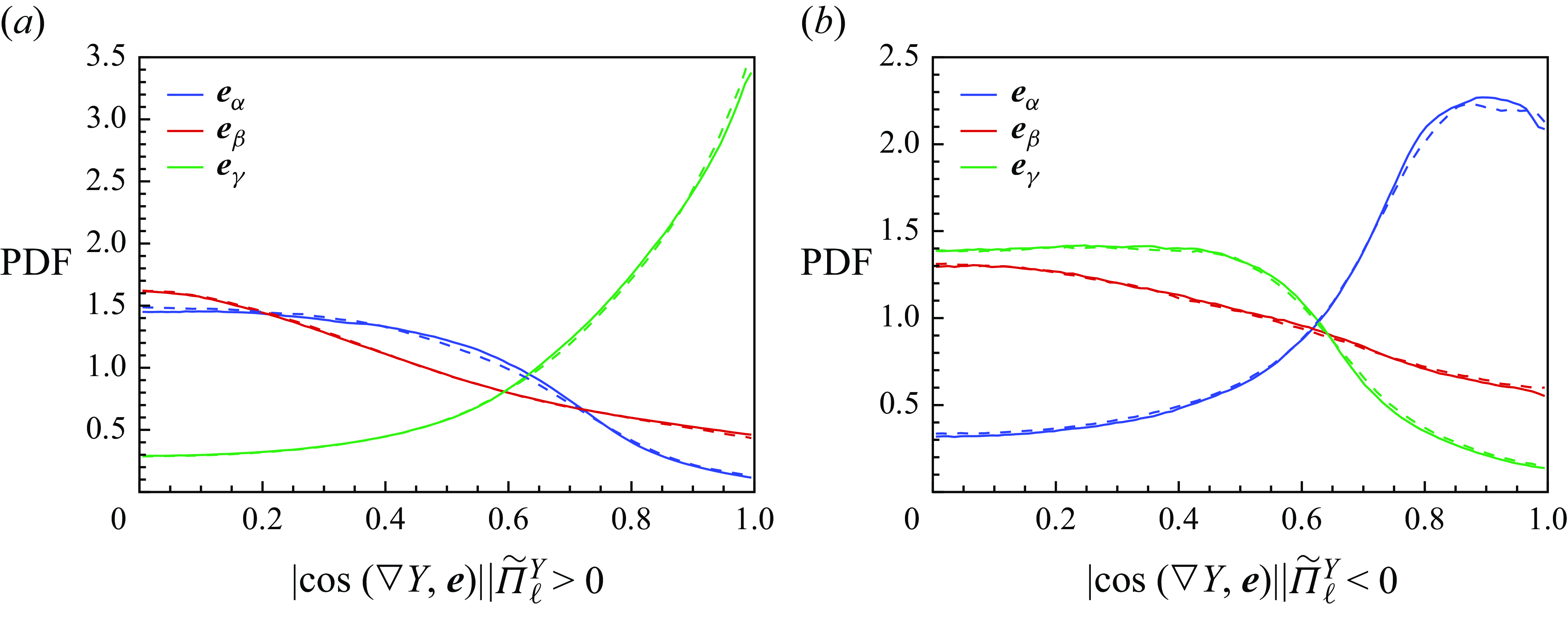
Figure 13. The alignment between the scalar gradient and the strain rate eigenvectors at $\widehat {t}=5$
, both filtered at
$\widehat {t}=5$
, both filtered at $\ell =64\eta$
. Panel (a) is conditional on the positive subset of
$\ell =64\eta$
. Panel (a) is conditional on the positive subset of $\widetilde {\Pi }_\ell ^Y$
, while panel (b) is conditional on the negative subset. The results for both the low-At (solid lines) and mid-At (dashed lines) cases are similar.
$\widetilde {\Pi }_\ell ^Y$
, while panel (b) is conditional on the negative subset. The results for both the low-At (solid lines) and mid-At (dashed lines) cases are similar.
5. Anisotropy in RT scalar transfer
A defining feature of RT turbulence is the persistence of anisotropy, not only in field variables like velocity and scalar gradient but also in the scalar transfer across scales. In this section we examine the directional anisotropy of $\widetilde {\Pi }_\ell ^Y$
at different scales and assess whether the nonlinear model accurately captures this anisotropic behaviour.
$\widetilde {\Pi }_\ell ^Y$
at different scales and assess whether the nonlinear model accurately captures this anisotropic behaviour.
Figure 14 shows the directional anisotropy for the velocity, vorticity and scalar gradient fields at $\widehat {t}=5$
, using the spectra of their three components. In figure 14(a) the velocity components reveal that at large and intermediate scales (small to intermediate
$\widehat {t}=5$
, using the spectra of their three components. In figure 14(a) the velocity components reveal that at large and intermediate scales (small to intermediate $k_\ell \equiv L_z/\ell$
), the vertical energy content is greater than the horizontal. However, at small scales, the horizontal and vertical energy contents nearly converge. Although some deviations are observed in the mid-At
$k_\ell \equiv L_z/\ell$
), the vertical energy content is greater than the horizontal. However, at small scales, the horizontal and vertical energy contents nearly converge. Although some deviations are observed in the mid-At $y$
components, these appear to be transient. For the vorticity spectra, a similar pattern of large-scale anisotropy and small-scale isotropy is observed, with the large-scale vertical enstrophy content being smaller than the horizontal components. A
$y$
components, these appear to be transient. For the vorticity spectra, a similar pattern of large-scale anisotropy and small-scale isotropy is observed, with the large-scale vertical enstrophy content being smaller than the horizontal components. A $k_\ell ^{1/3}$
scaling behaviour is seen at intermediate scales, consistent with the
$k_\ell ^{1/3}$
scaling behaviour is seen at intermediate scales, consistent with the $k_\ell ^{-5/3}$
scaling in the KE spectra.
$k_\ell ^{-5/3}$
scaling in the KE spectra.
Although both the velocity and vorticity fields exhibit directional anisotropy, the anisotropy is much more pronounced in the velocity field. For the specific KE, the ratio of the total $z$
component to the total
$z$
component to the total $x$
component is 3.9 for the low-At case and 3.6 for the mid-At case. In contrast, for the vorticity field, these ratios are 0.91 and 0.94, respectively. This difference arises because small-scale components dominate the vorticity field, whereas large-scale components are more significant in the velocity field. Consequently, the small-scale isotropy of the vorticity field results in reduced directional anisotropy compared with the velocity field.
$x$
component is 3.9 for the low-At case and 3.6 for the mid-At case. In contrast, for the vorticity field, these ratios are 0.91 and 0.94, respectively. This difference arises because small-scale components dominate the vorticity field, whereas large-scale components are more significant in the velocity field. Consequently, the small-scale isotropy of the vorticity field results in reduced directional anisotropy compared with the velocity field.
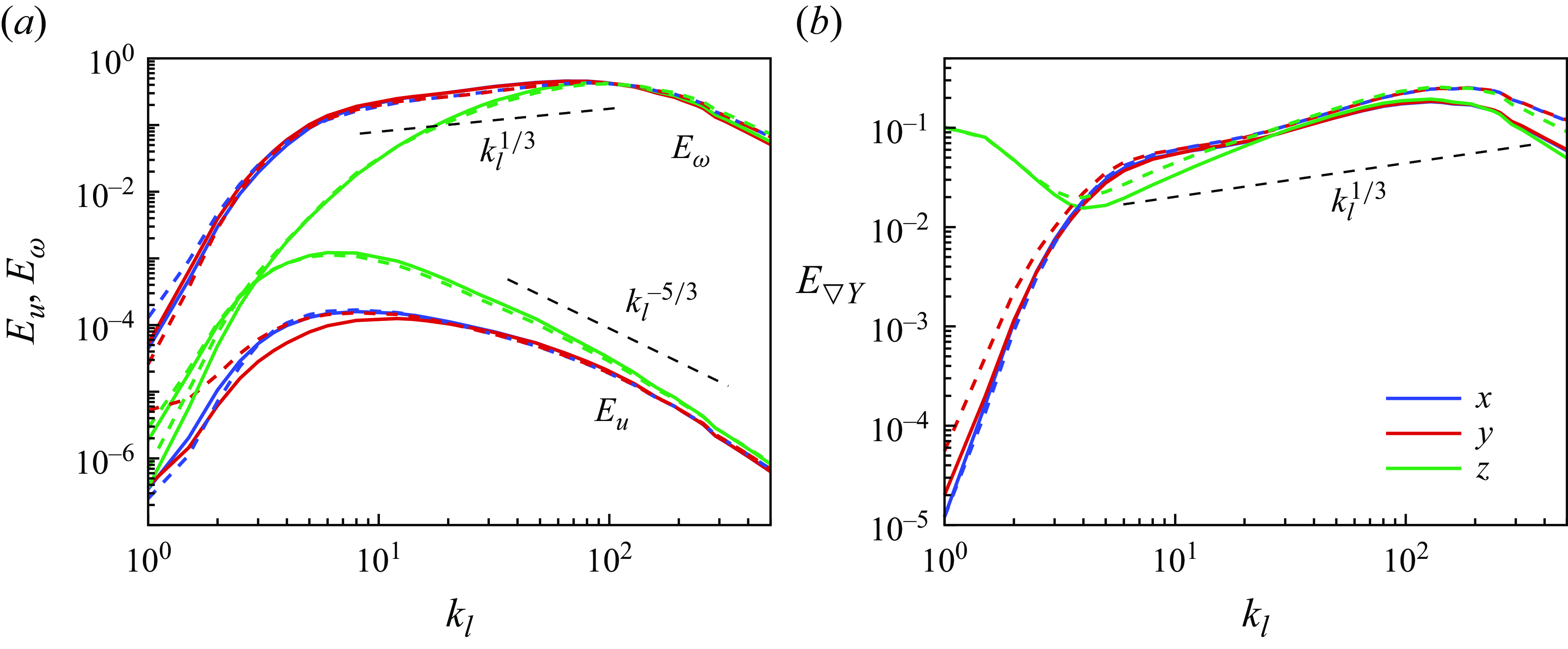
Figure 14. The filtering spectra for the (a) velocity, vorticity and (b) scalar gradient fields at $\widehat {t}=5$
, where
$\widehat {t}=5$
, where $\ell$
is the filtering width and
$\ell$
is the filtering width and $k_\ell = L_z/\ell$
. Solid and dashed lines represent the low-At and mid-At cases, respectively, and black dashed lines represent the reference scalings
$k_\ell = L_z/\ell$
. Solid and dashed lines represent the low-At and mid-At cases, respectively, and black dashed lines represent the reference scalings $k_\ell ^{-5/3}$
,
$k_\ell ^{-5/3}$
, $k_\ell ^{1/3}$
and
$k_\ell ^{1/3}$
and $k_\ell ^{1/3}$
. The KE and enstrophy are normalised by the corresponding mean values.
$k_\ell ^{1/3}$
. The KE and enstrophy are normalised by the corresponding mean values.
Figure 14(b) shows the spectra of the three components of the scalar gradient. The relative magnitudes of the horizontal to vertical components exhibit non-monotonic behaviour. At large scales, the vertical scalar gradient dominates due to the initial stratification, which persists at this time since the mixing region has not yet reached the walls. The $z$
component of
$z$
component of $E_{\nabla Y}$
then decreases with increasing
$E_{\nabla Y}$
then decreases with increasing $k_\ell$
, reaching a turning point around
$k_\ell$
, reaching a turning point around $k_\ell = 4$
for both the low-At and mid-At cases, a wavenumber comparable to the mixing width at
$k_\ell = 4$
for both the low-At and mid-At cases, a wavenumber comparable to the mixing width at $\widehat {t}=5$
. Beyond this wavenumber, both horizontal and vertical components of
$\widehat {t}=5$
. Beyond this wavenumber, both horizontal and vertical components of $E_{\nabla Y}$
increase with
$E_{\nabla Y}$
increase with $k_\ell$
, with the vertical component slightly smaller than the horizontal. The scaling appears to be slightly greater than the expected
$k_\ell$
, with the vertical component slightly smaller than the horizontal. The scaling appears to be slightly greater than the expected $k_\ell ^{1/3}$
behaviour, which corresponds to a
$k_\ell ^{1/3}$
behaviour, which corresponds to a $k_\ell ^{-5/3}$
scaling in the mass fraction spectrum. At the smallest scales, the spectra
$k_\ell ^{-5/3}$
scaling in the mass fraction spectrum. At the smallest scales, the spectra $E_{\nabla Y}$
decrease due to diffusion-induced dissipation. Overall, combining the observations from figure 14, we see that directional anisotropy persists at large scales but diminishes at smaller scales, in line with Kolmogorov’s assumption of small-scale equilibrium. In addition, the transition to isotropy occurs at larger scales (i.e. smaller transitional
$E_{\nabla Y}$
decrease due to diffusion-induced dissipation. Overall, combining the observations from figure 14, we see that directional anisotropy persists at large scales but diminishes at smaller scales, in line with Kolmogorov’s assumption of small-scale equilibrium. In addition, the transition to isotropy occurs at larger scales (i.e. smaller transitional $k_\ell$
) for the scalar gradient compared with the velocity and vorticity fields.
$k_\ell$
) for the scalar gradient compared with the velocity and vorticity fields.
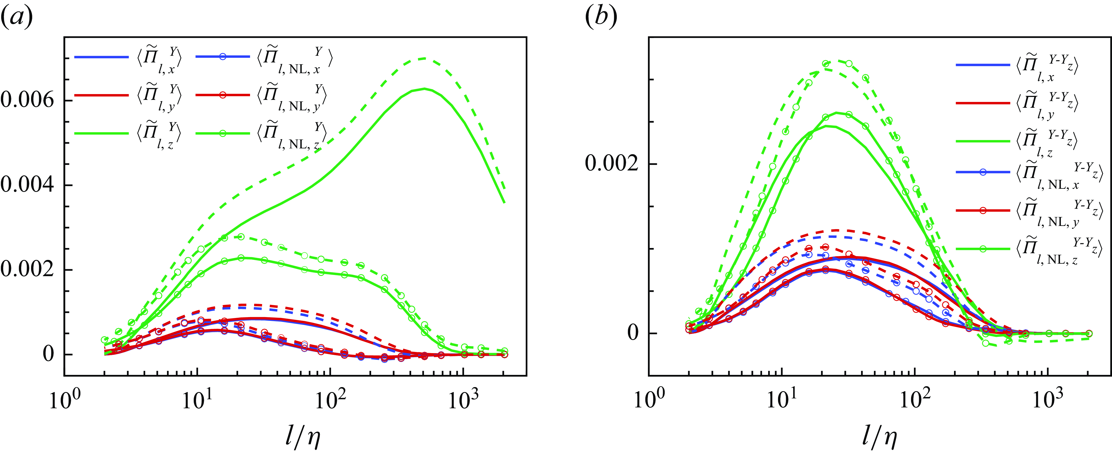
Figure 15. (a) The mean values of the three components of scalar variance transfer and the corresponding three components of the nonlinear model (marker with open circles), for both the low-At and mid-At cases at $\widehat {t}=5$
. (b) Similar results, with both
$\widehat {t}=5$
. (b) Similar results, with both $\widetilde {\Pi }_\ell ^Y$
and its nonlinear model evaluated with the mass fraction field
$\widetilde {\Pi }_\ell ^Y$
and its nonlinear model evaluated with the mass fraction field $Y$
replaced by
$Y$
replaced by $Y-Y_z\equiv Y-\langle Y\rangle _{xy}$
, i.e. subtracting the horizontal mean profile.
$Y-Y_z\equiv Y-\langle Y\rangle _{xy}$
, i.e. subtracting the horizontal mean profile.
We further investigate the anisotropy of the scalar transfer term. Figure 15(a) shows the spatial mean of the scalar variance flux components $\widetilde {\Pi }^Y_{\ell ,i} = -\overline {\rho }_\ell \partial _{i} \widetilde {Y}_\ell \widetilde {\tau }_\ell (Y, u_{i})$
, where
$\widetilde {\Pi }^Y_{\ell ,i} = -\overline {\rho }_\ell \partial _{i} \widetilde {Y}_\ell \widetilde {\tau }_\ell (Y, u_{i})$
, where $i=x, y$
and
$i=x, y$
and $z$
. For both the low-At and mid-At cases, the
$z$
. For both the low-At and mid-At cases, the $z$
-component
$z$
-component $\widetilde {\Pi }^Y_{\ell ,z}$
dominates over the horizontal components
$\widetilde {\Pi }^Y_{\ell ,z}$
dominates over the horizontal components $\widetilde {\Pi }^Y_{\ell ,x}$
and
$\widetilde {\Pi }^Y_{\ell ,x}$
and $\widetilde {\Pi }^Y_{\ell ,y}$
, specifically at large scales, while mean values of the two horizontal components are similar. This directional anisotropy reflects the influence of the initial density stratification and the gravitational acceleration field. The nonlinear model
$\widetilde {\Pi }^Y_{\ell ,y}$
, specifically at large scales, while mean values of the two horizontal components are similar. This directional anisotropy reflects the influence of the initial density stratification and the gravitational acceleration field. The nonlinear model $\widetilde {\Pi }^Y_{\ell ,\mathrm {NL}} = C_0\ell ^2 \overline {\rho } \widetilde {\mathcal {S}}^Y_\ell$
, shown in figure 15(a) with open circles, is able to capture the directional anisotropy only for
$\widetilde {\Pi }^Y_{\ell ,\mathrm {NL}} = C_0\ell ^2 \overline {\rho } \widetilde {\mathcal {S}}^Y_\ell$
, shown in figure 15(a) with open circles, is able to capture the directional anisotropy only for $\ell /\eta \lessapprox 10$
. However, at intermediate to large scales, the mean values of the nonlinear model deviate significantly from the simulation results, particularly for the vertical component. This deviation is expected because, for the anisotropic RT flow at relatively large scales, the assumptions underlying the nonlinear model, namely scale locality and the Taylor series expansion, become invalid, leading to substantial approximation errors. Potential remedies for this deviation include adopting the multi-scale gradient expansion (Eyink Reference Eyink2006), using higher-order Taylor expansions or employing the constant-coefficient spatial gradient model (Wang et al. Reference Wang, Yuan, Wang and Wang2022).
$\ell /\eta \lessapprox 10$
. However, at intermediate to large scales, the mean values of the nonlinear model deviate significantly from the simulation results, particularly for the vertical component. This deviation is expected because, for the anisotropic RT flow at relatively large scales, the assumptions underlying the nonlinear model, namely scale locality and the Taylor series expansion, become invalid, leading to substantial approximation errors. Potential remedies for this deviation include adopting the multi-scale gradient expansion (Eyink Reference Eyink2006), using higher-order Taylor expansions or employing the constant-coefficient spatial gradient model (Wang et al. Reference Wang, Yuan, Wang and Wang2022).
Without the additional complexities mentioned above, we can still enhance the performance of the nonlinear model by considering only the fluctuation part of the mass fraction field, $Y - Y_z \equiv Y - \langle Y \rangle _{xy}$
. The mean vertical profile
$Y - Y_z \equiv Y - \langle Y \rangle _{xy}$
. The mean vertical profile $Y_z$
can be approximated as
$Y_z$
can be approximated as $Y_z \approx {1}/{2} [ 1 + \mathrm {erf} (z/h(t) ) ]$
(Boffetta, De Lillo & Musacchio Reference Boffetta, De Lillo and Musacchio2010), where
$Y_z \approx {1}/{2} [ 1 + \mathrm {erf} (z/h(t) ) ]$
(Boffetta, De Lillo & Musacchio Reference Boffetta, De Lillo and Musacchio2010), where $h(t) = \alpha \mathrm {At}\,g t^2$
represents the height of the mixing width. By subtracting the mean vertical profile, we partially mitigate the dependence on the initial density stratification and reduce the external anisotropy of the system. Figure 15(b) displays the mean values of the components of
$h(t) = \alpha \mathrm {At}\,g t^2$
represents the height of the mixing width. By subtracting the mean vertical profile, we partially mitigate the dependence on the initial density stratification and reduce the external anisotropy of the system. Figure 15(b) displays the mean values of the components of $\widetilde {\Pi }_\ell ^Y$
and their nonlinear model for the fluctuating mass fraction field. Compared with figure 15(a), the nonlinear model provides a better approximation of the scalar variance flux, particularly for the vertical component at large scales. Thus, the nonlinear model effectively captures the directional anisotropy of
$\widetilde {\Pi }_\ell ^Y$
and their nonlinear model for the fluctuating mass fraction field. Compared with figure 15(a), the nonlinear model provides a better approximation of the scalar variance flux, particularly for the vertical component at large scales. Thus, the nonlinear model effectively captures the directional anisotropy of $\widetilde {\Pi }^{Y-Y_z}_\ell$
. The remaining component,
$\widetilde {\Pi }^{Y-Y_z}_\ell$
. The remaining component, $\widetilde {\Pi }^Y - \widetilde {\Pi }^{Y-Y_z}_\ell$
, still requires modelling, such as through the eddy viscosity model or its variants (Kokkinakis et al. Reference Kokkinakis, Drikakis, Youngs and Williams2015; Zhou Reference Zhou2017b
), which we leave for future work. Figure 15 highlights the benefit of isolating the fluctuating part of the scalar field from its horizontal mean profile when developing numerical models for scalar transfer in RT turbulence.
$\widetilde {\Pi }^Y - \widetilde {\Pi }^{Y-Y_z}_\ell$
, still requires modelling, such as through the eddy viscosity model or its variants (Kokkinakis et al. Reference Kokkinakis, Drikakis, Youngs and Williams2015; Zhou Reference Zhou2017b
), which we leave for future work. Figure 15 highlights the benefit of isolating the fluctuating part of the scalar field from its horizontal mean profile when developing numerical models for scalar transfer in RT turbulence.
6. Conclusions
In this paper we have investigated the multi-scale dynamics of scalar mixing in RT turbulence for low ( $\mathrm {At}=0.15$
) and moderate (
$\mathrm {At}=0.15$
) and moderate ( $\mathrm {At}=0.5$
) Atwood number cases. The scalar variance flux across scales,
$\mathrm {At}=0.5$
) Atwood number cases. The scalar variance flux across scales, $\widetilde {\Pi }^Y_\ell$
, is on average positive, thus transfers scalar variance from large to small scales. A nonlinear model of
$\widetilde {\Pi }^Y_\ell$
, is on average positive, thus transfers scalar variance from large to small scales. A nonlinear model of $\widetilde {\Pi }^Y_\ell$
shows that its magnitude depends primarily on the symmetric strain rate tensor, rather than the vorticity fields. However, locally, the scalar variance flux can become negative, partly due to vorticity-induced alignment of the scalar normal direction with the most expansive eigenvector of the strain field. Therefore, while the symmetric velocity gradient primarily influences the magnitude of
$\widetilde {\Pi }^Y_\ell$
shows that its magnitude depends primarily on the symmetric strain rate tensor, rather than the vorticity fields. However, locally, the scalar variance flux can become negative, partly due to vorticity-induced alignment of the scalar normal direction with the most expansive eigenvector of the strain field. Therefore, while the symmetric velocity gradient primarily influences the magnitude of $\widetilde {\Pi }^Y_\ell$
, the anti-symmetric velocity gradient also contributes to generating negative values of
$\widetilde {\Pi }^Y_\ell$
, the anti-symmetric velocity gradient also contributes to generating negative values of $\widetilde {\Pi }^Y_\ell$
. Similar results are also observed in simulations with high Atwood and high Reynolds numbers. Additionally, we demonstrate the directional anisotropy in RT turbulence, showing that the nonlinear model accurately captures the anisotropic behaviour of the scalar transfer term when focusing on the fluctuating component of the scalar field, with the horizontal mean profile subtracted.
$\widetilde {\Pi }^Y_\ell$
. Similar results are also observed in simulations with high Atwood and high Reynolds numbers. Additionally, we demonstrate the directional anisotropy in RT turbulence, showing that the nonlinear model accurately captures the anisotropic behaviour of the scalar transfer term when focusing on the fluctuating component of the scalar field, with the horizontal mean profile subtracted.
In the temporal evolution of RT mixing, we observe that during the self-similar stage, the statistics of various kinematic and dynamical quantities remain stable over time. For instance, the interfacial area of the scalar isosurface increases linearly with time, while the fractal dimensions of the isosurface fluctuate around 2.41 for the low-At case and 2.46 for the mid-At case. The change in isosurface area is primarily governed by the scalar element stretching, $\mathcal {S}^Y$
. Furthermore, we establish a similarity between
$\mathcal {S}^Y$
. Furthermore, we establish a similarity between $\mathcal {S}^Y$
and the mean scalar dissipation,
$\mathcal {S}^Y$
and the mean scalar dissipation, $\mathcal {\varepsilon }^Y$
, through the preferential alignment of the scalar normal with the eigenvector corresponding to the most compressive eigenvalue of the strain field. This alignment is shown to be reinforced by the rate of change of the scalar normal direction due to the straining term, while the vorticity term tends to weaken this alignment.
$\mathcal {\varepsilon }^Y$
, through the preferential alignment of the scalar normal with the eigenvector corresponding to the most compressive eigenvalue of the strain field. This alignment is shown to be reinforced by the rate of change of the scalar normal direction due to the straining term, while the vorticity term tends to weaken this alignment.
The evolution of the scalar field is further investigated using a spatial coarse-graining approach to analyse the cross-scale transfer of scalar variance, in particular the transfer term $\widetilde {\Pi }^Y_\ell \equiv -\overline {\rho } \partial _j \widetilde {Y} \widetilde {\tau }(Y, u_j)$
. Numerical results show that the spatial mean of
$\widetilde {\Pi }^Y_\ell \equiv -\overline {\rho } \partial _j \widetilde {Y} \widetilde {\tau }(Y, u_j)$
. Numerical results show that the spatial mean of $\widetilde {\Pi }^Y_\ell$
is consistently positive, indicating a downscale transfer of scalar variance. The conditional mean analysis reveals that
$\widetilde {\Pi }^Y_\ell$
is consistently positive, indicating a downscale transfer of scalar variance. The conditional mean analysis reveals that $\widetilde {\Pi }^Y_\ell$
is positively correlated with the filtered strain, with no significant correlation with the filtered vorticity field. This behaviour is well captured by the nonlinear model
$\widetilde {\Pi }^Y_\ell$
is positively correlated with the filtered strain, with no significant correlation with the filtered vorticity field. This behaviour is well captured by the nonlinear model $\widetilde {\Pi }^Y_\ell \approx \widetilde {\Pi }^Y_{\ell , \mathrm {NL}} =-C_0\ell ^2 \overline {\rho } \nabla \overline {Y}\cdot \overline {\boldsymbol {S}}\cdot \nabla \overline {Y} \approx C_0 \ell ^2 \overline {\rho } \widetilde {\mathcal {S}}^Y$
, which is validated through joint PDFs and correlation coefficients.
$\widetilde {\Pi }^Y_\ell \approx \widetilde {\Pi }^Y_{\ell , \mathrm {NL}} =-C_0\ell ^2 \overline {\rho } \nabla \overline {Y}\cdot \overline {\boldsymbol {S}}\cdot \nabla \overline {Y} \approx C_0 \ell ^2 \overline {\rho } \widetilde {\mathcal {S}}^Y$
, which is validated through joint PDFs and correlation coefficients.
Additionally, the role of vorticity in scalar transfer is primarily associated with the negative values of $\widetilde {\Pi }^Y_\ell$
, which indicate an inverse transfer from small to large scales. These negative values are predominantly found in the first quadrant of the filtered
$\widetilde {\Pi }^Y_\ell$
, which indicate an inverse transfer from small to large scales. These negative values are predominantly found in the first quadrant of the filtered $\overline {Q}_\ell{-}\overline {R}_\ell$
space, where vorticity is dominant. Furthermore, negative
$\overline {Q}_\ell{-}\overline {R}_\ell$
space, where vorticity is dominant. Furthermore, negative $\widetilde {\Pi }^Y_\ell$
is due to changes in the preferential alignment statistics between
$\widetilde {\Pi }^Y_\ell$
is due to changes in the preferential alignment statistics between $\nabla \overline {Y}_\ell$
and the strain eigensystem. While the overall statistics indicate that
$\nabla \overline {Y}_\ell$
and the strain eigensystem. While the overall statistics indicate that $\nabla \overline {Y}$
is mostly parallel to
$\nabla \overline {Y}$
is mostly parallel to $\boldsymbol {e}_{ \gamma }$
, the results conditional on negative
$\boldsymbol {e}_{ \gamma }$
, the results conditional on negative $\widetilde {\Pi }^Y_\ell$
reveal an alignment between
$\widetilde {\Pi }^Y_\ell$
reveal an alignment between $\nabla \overline {Y}$
and
$\nabla \overline {Y}$
and $\boldsymbol {e}_{\alpha }$
. This shift in alignment is attributed to the vorticity-induced rotation of the scalar normal direction, resulting in negative scalar stretching,
$\boldsymbol {e}_{\alpha }$
. This shift in alignment is attributed to the vorticity-induced rotation of the scalar normal direction, resulting in negative scalar stretching, $\widetilde {\mathcal {S}}^Y_\ell \lt 0$
, which in turn leads to negative
$\widetilde {\mathcal {S}}^Y_\ell \lt 0$
, which in turn leads to negative $\widetilde {\Pi }^Y_\ell$
. Thus, both the strain rate and vorticity fields play crucial roles in influencing scalar variance transfer across scales.
$\widetilde {\Pi }^Y_\ell$
. Thus, both the strain rate and vorticity fields play crucial roles in influencing scalar variance transfer across scales.
Finally, we investigate the directional anisotropy in RT turbulence, specifically focusing on the anisotropy of the scalar transfer term. A key finding is that directional anisotropy is pronounced at large scales but diminishes at smaller scales. The scalar variance transfer displays significant anisotropy among its components, and the nonlinear model fails to capture this behaviour. However, when the horizontally averaged profile of the mass fraction is subtracted, the directional anisotropy decreases, leading to improved predictions from the nonlinear model. Therefore, it is beneficial to treat the horizontally averaged mass fraction profile and the fluctuating component separately when modelling RT scalar mixing.
Funding.
This work is supported by the National Natural Science Foundation of China (Nos. 12202270, 12102258 and 12372264), and the China Postdoctoral Science Foundation (No. 2023M742269). The authors also appreciate the computational support from the Centre for High Performance Computing at Shanghai Jiao Tong University.
Declaration of interests.
The authors report no conflict of interest.
Appendix A. Temporal evolution of the Kolmogorov scale in RT simulations
Figure 16 shows the evolution of the Kolmogorov scale, $\eta$
, defined in table 1, normalised by the grid size. In both the low-At and mid-At cases,
$\eta$
, defined in table 1, normalised by the grid size. In both the low-At and mid-At cases, $\eta$
exhibits a sharp decrease before
$\eta$
exhibits a sharp decrease before $\widehat {t}\lt 1$
. After this point, the rate of decrease slows and gradually stabilises after
$\widehat {t}\lt 1$
. After this point, the rate of decrease slows and gradually stabilises after $\widehat {t}\gt 2$
, corresponding to the self-similar stage of RT evolution, as indicated in figure 2. Throughout the entire evolution, the criterion
$\widehat {t}\gt 2$
, corresponding to the self-similar stage of RT evolution, as indicated in figure 2. Throughout the entire evolution, the criterion $k_{\mathrm {max}}\eta \geqslant 1.5$
is met in both simulations, ensuring sufficient resolution to capture the small turbulent scales (Yeung & Pope Reference Yeung and Pope1989).
$k_{\mathrm {max}}\eta \geqslant 1.5$
is met in both simulations, ensuring sufficient resolution to capture the small turbulent scales (Yeung & Pope Reference Yeung and Pope1989).
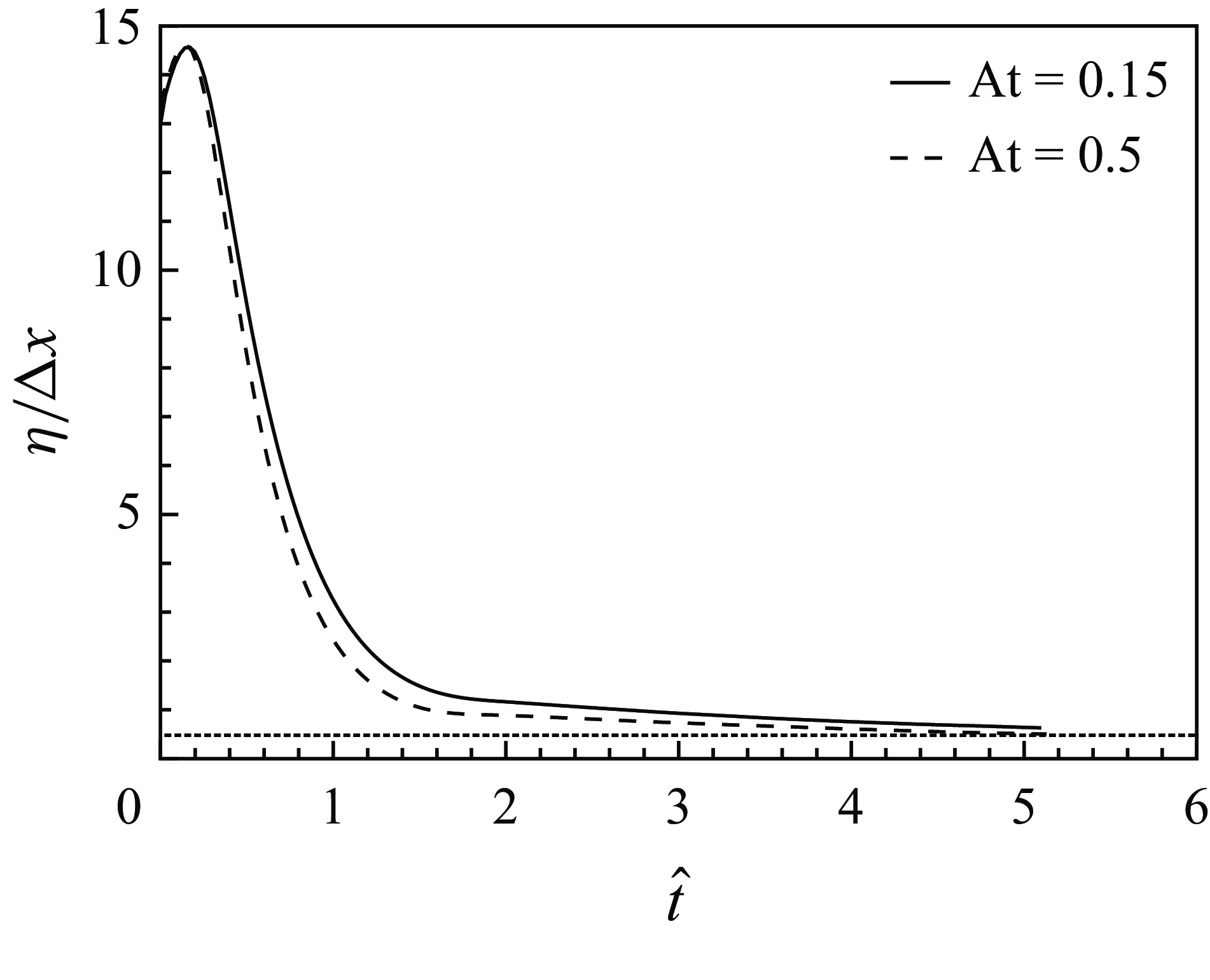
Figure 16. Temporal evolution of the Kolmogorov scale, $\eta$
, normalised by the grid size
$\eta$
, normalised by the grid size $\Delta x$
. The dotted line marks the threshold for an adequate resolution of the small scales in turbulent flows,
$\Delta x$
. The dotted line marks the threshold for an adequate resolution of the small scales in turbulent flows, $\eta /\Delta x=1.5/\pi$
, or
$\eta /\Delta x=1.5/\pi$
, or $k_{\mathrm {max}}\eta \geqslant 1.5$
, where
$k_{\mathrm {max}}\eta \geqslant 1.5$
, where $k_{\mathrm {max}}$
is the maximum resolved wavenumber.
$k_{\mathrm {max}}$
is the maximum resolved wavenumber.
Appendix B. Fractal dimension of isoscalar surfaces
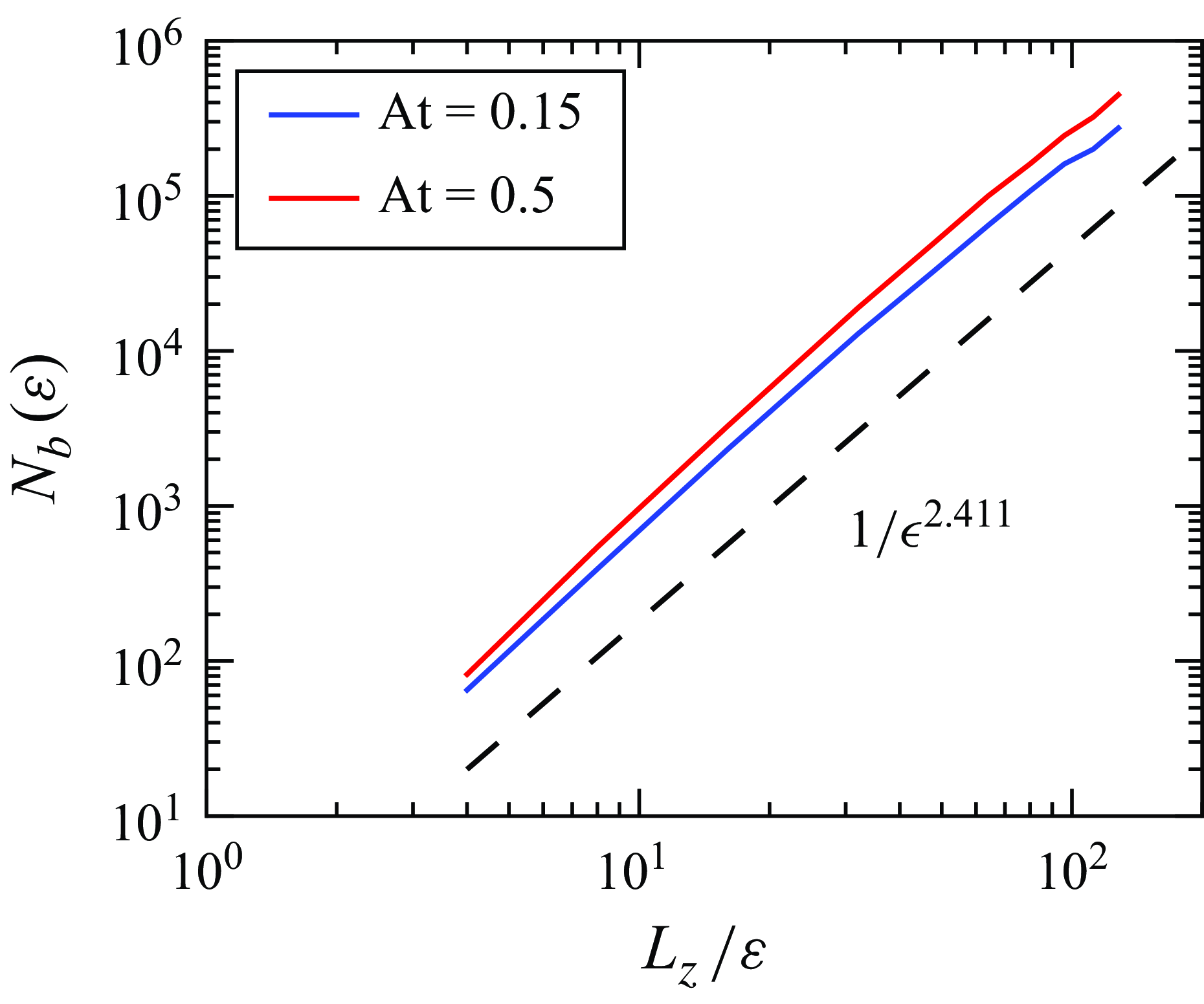
Figure 17. The fractal dimensions for the low-At and mid-At $Y=0.5$
isosurfaces determined using the box-counting algorithm. Here,
$Y=0.5$
isosurfaces determined using the box-counting algorithm. Here, $\varepsilon$
represents the box size and
$\varepsilon$
represents the box size and $N_b(\varepsilon )$
is the total number of boxes required to fully cover the isosurface with non-overlapping boxes of size
$N_b(\varepsilon )$
is the total number of boxes required to fully cover the isosurface with non-overlapping boxes of size $\varepsilon$
. The scaling exponents
$\varepsilon$
. The scaling exponents $D_3$
represent the fractal dimensions of the isosurfaces embedded in 3-D space, calculated to be 2.411 for the low-At case and 2.474 for the mid-At case.
$D_3$
represent the fractal dimensions of the isosurfaces embedded in 3-D space, calculated to be 2.411 for the low-At case and 2.474 for the mid-At case.

Figure 18. The joint PDFs between the scalar stretching $\mathcal {S}^Y$
and scalar dissipation
$\mathcal {S}^Y$
and scalar dissipation $\varepsilon ^Y$
at
$\varepsilon ^Y$
at $\widehat {t}=5$
for the (a) low-At and (b) mid-At cases. Both the
$\widehat {t}=5$
for the (a) low-At and (b) mid-At cases. Both the $\mathcal {S}^Y$
and
$\mathcal {S}^Y$
and $\varepsilon ^Y$
fields are normalised by their respective maximum value.
$\varepsilon ^Y$
fields are normalised by their respective maximum value.
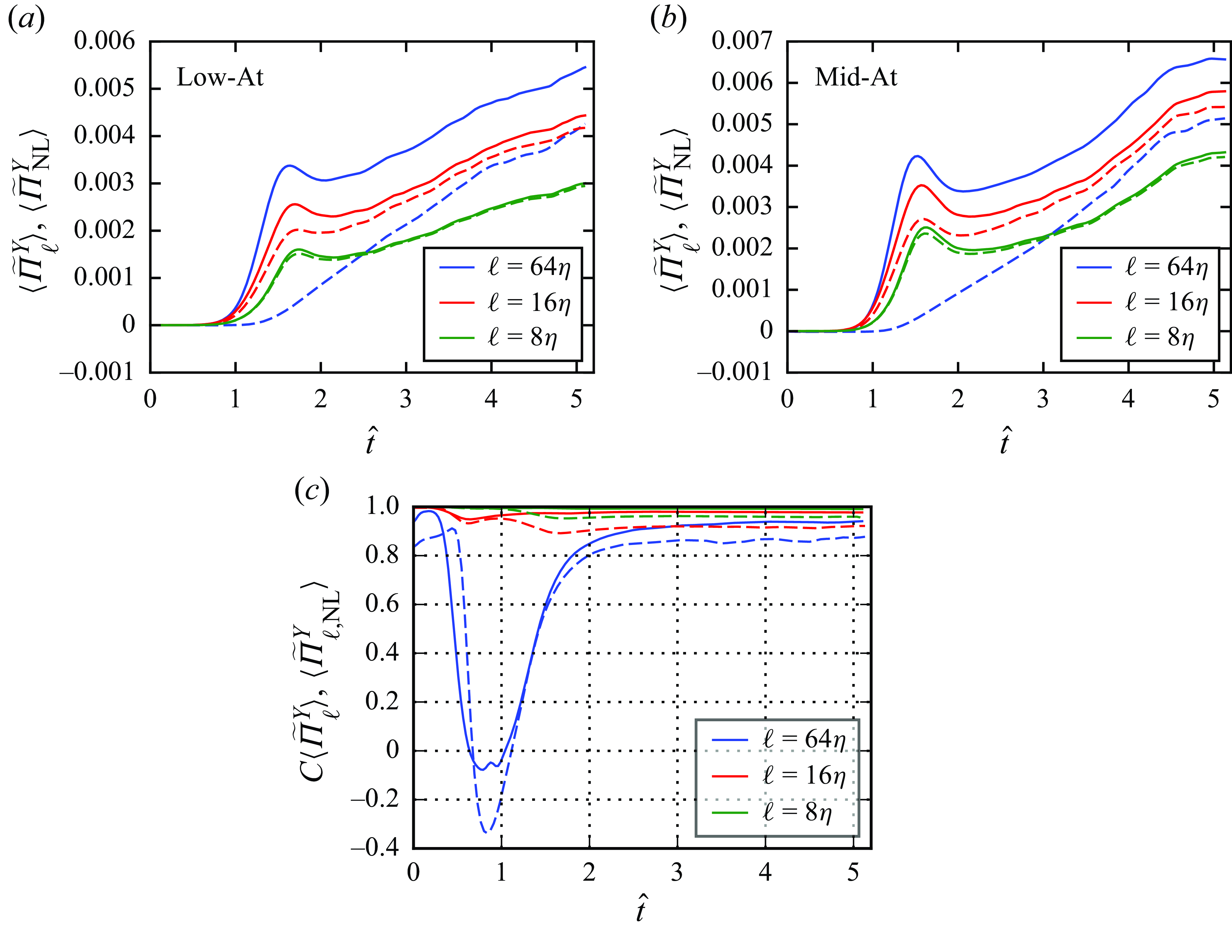
Figure 19. (a) Temporal evolution of the mean scalar variance flux and its nonlinear model for the low-At case, where solid lines represent $\langle \Pi _\ell ^Y \rangle$
and dashed lines represent
$\langle \Pi _\ell ^Y \rangle$
and dashed lines represent $\langle \Pi _{\mathrm {NL}}^Y \rangle$
. Panel (b) presents similar results for the mid-At case. Panel (c) shows the correlation coefficients between
$\langle \Pi _{\mathrm {NL}}^Y \rangle$
. Panel (b) presents similar results for the mid-At case. Panel (c) shows the correlation coefficients between $\langle \Pi _\ell ^Y \rangle$
and
$\langle \Pi _\ell ^Y \rangle$
and $\langle \Pi _{\mathrm {NL}}^Y \rangle$
, with solid and dashed lines corresponding to the low-At and mid-At cases, respectively.
$\langle \Pi _{\mathrm {NL}}^Y \rangle$
, with solid and dashed lines corresponding to the low-At and mid-At cases, respectively.
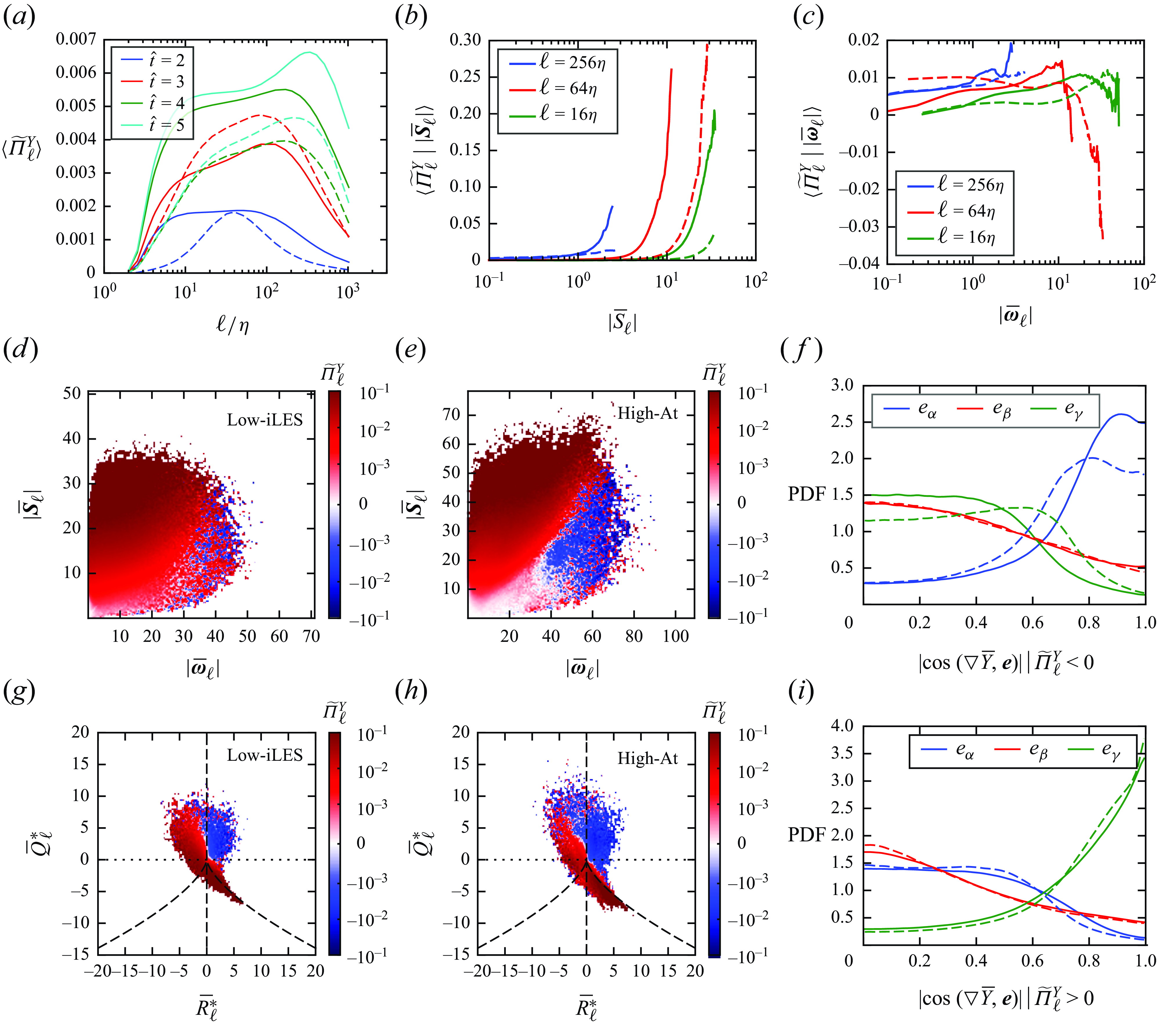
Figure 20. Scalar variance transfer statistics for the low-iLES (solid lines) and high-At (dashed lines) cases are presented. Panel (a) shows the mean value of the scalar variance transfer term over filter widths at $\widehat {t}=2-5$
. Panels (b) and (c) show the mean value of
$\widehat {t}=2-5$
. Panels (b) and (c) show the mean value of $\widetilde {\Pi }_\ell ^Y$
conditioned on the filtered strain rate and vorticity magnitudes, respectively. Panels (d,e) and (g,h) show the mean value of
$\widetilde {\Pi }_\ell ^Y$
conditioned on the filtered strain rate and vorticity magnitudes, respectively. Panels (d,e) and (g,h) show the mean value of $\widetilde {\Pi }_\ell ^Y$
conditioned on the joint PDFs of
$\widetilde {\Pi }_\ell ^Y$
conditioned on the joint PDFs of $|\overline {S}_\ell |$
−
$|\overline {S}_\ell |$
− $|\overline {\boldsymbol {\omega }}_\ell |$
and
$|\overline {\boldsymbol {\omega }}_\ell |$
and $\overline {Q}_\ell$
−
$\overline {Q}_\ell$
− $\overline {R}_\ell$
, respectively, for both the low-iLES and high-At cases. Finally, (f) and (i) illustrate the alignment between the filtered scalar gradient and the strain rate eigensystem for the negative and positive portions of
$\overline {R}_\ell$
, respectively, for both the low-iLES and high-At cases. Finally, (f) and (i) illustrate the alignment between the filtered scalar gradient and the strain rate eigensystem for the negative and positive portions of $\widetilde {\Pi }_\ell ^Y$
. The results in panels (b)–(i) are obtained at
$\widetilde {\Pi }_\ell ^Y$
. The results in panels (b)–(i) are obtained at $\widehat {t}=5$
.
$\widehat {t}=5$
.
Figure 17 illustrates the application of the box-counting algorithm to determine fractal dimension, $D_3$
, of the
$D_3$
, of the $Y=0.5$
isosurface shown in figure 3. The algorithm partitions the 3-D space into non-overlapping cubes of varying sizes,
$Y=0.5$
isosurface shown in figure 3. The algorithm partitions the 3-D space into non-overlapping cubes of varying sizes, $\varepsilon$
. For each partition with a fixed
$\varepsilon$
. For each partition with a fixed $\varepsilon$
, the total number of cubes required to fully cover the isoscalar surface is denoted as
$\varepsilon$
, the total number of cubes required to fully cover the isoscalar surface is denoted as $N_b(\varepsilon )$
. If the isosurface exhibits self-similar fractal characteristics, the relationship
$N_b(\varepsilon )$
. If the isosurface exhibits self-similar fractal characteristics, the relationship $N_b(\varepsilon ) \sim (1/\varepsilon )^{D_3}$
holds, allowing the determination of the fractal dimension
$N_b(\varepsilon ) \sim (1/\varepsilon )^{D_3}$
holds, allowing the determination of the fractal dimension $D_3$
of the isosurface within the 3-D space.
$D_3$
of the isosurface within the 3-D space.
Figure 17 shows that the isosurfaces for both the low-At and mid-At cases at $\widehat {t}=5$
are self-similar, with fractal dimensions of 2.411 and 2.474, respectively. The slightly higher fractal dimension of the mid-At isosurface corresponds to the larger surface area shown in figure 2(a), indicating a more corrugated surface due to the larger density contrast and greater potential energy release in the mid-At case.
$\widehat {t}=5$
are self-similar, with fractal dimensions of 2.411 and 2.474, respectively. The slightly higher fractal dimension of the mid-At isosurface corresponds to the larger surface area shown in figure 2(a), indicating a more corrugated surface due to the larger density contrast and greater potential energy release in the mid-At case.
Appendix C. Correlation between surface stretching and scalar dissipation
In addition to the correlation between the temporal evolution of spatial mean values of surface stretching $\mathcal {S}^Y$
and scalar dissipation
$\mathcal {S}^Y$
and scalar dissipation $\varepsilon ^Y$
shown in figure 4, there is also a spatial correlation, as depicted in figure 18, with correlation coefficients of 0.95 and 0.93 for the low-At and mid-At cases, respectively. This high correlation arises from the preferential alignment between
$\varepsilon ^Y$
shown in figure 4, there is also a spatial correlation, as depicted in figure 18, with correlation coefficients of 0.95 and 0.93 for the low-At and mid-At cases, respectively. This high correlation arises from the preferential alignment between $\nabla Y$
and
$\nabla Y$
and $\boldsymbol {e}_\gamma$
, as indicated in (3.7).
$\boldsymbol {e}_\gamma$
, as indicated in (3.7).
Appendix D. Temporal evolution of the nonlinear model prediction
To further evaluate the nonlinear model approximation of the scalar variance flux, complementing the results in figure 10, we present the temporal evolution of the mean scalar variance flux and its nonlinear model in figures 19(a) and 19(b), along with the correlation coefficient between the two in figure 19(c). The results show that for both low- and mid-At cases, $\langle \Pi _{\mathrm {NL}}^Y \rangle$
approaches
$\langle \Pi _{\mathrm {NL}}^Y \rangle$
approaches $\langle \Pi _\ell ^Y \rangle$
as the filter width decreases. Additionally, the correlation coefficient between the flux and the nonlinear model remains above 0.8 for
$\langle \Pi _\ell ^Y \rangle$
as the filter width decreases. Additionally, the correlation coefficient between the flux and the nonlinear model remains above 0.8 for $\widehat {t} \gt 2$
, when RT turbulence is in the self-similar regime. These findings, presented in figure 19, further confirm the nonlinear model’s good approximation of the scalar variance flux in RT turbulence.
$\widehat {t} \gt 2$
, when RT turbulence is in the self-similar regime. These findings, presented in figure 19, further confirm the nonlinear model’s good approximation of the scalar variance flux in RT turbulence.
Appendix E. The case of high Atwood and high Reynolds numbers
In this section we demonstrate that the main findings of the paper are applicable to both high Atwood number and high Reynolds number RT turbulence. Statistics of the scalar variance transfer term, $\widetilde {\Pi }^Y_\ell$
, for the high-At and low-iLES cases, as detailed in table 1, are shown in figure 20. The results confirm that the mean value of
$\widetilde {\Pi }^Y_\ell$
, for the high-At and low-iLES cases, as detailed in table 1, are shown in figure 20. The results confirm that the mean value of $\widetilde {\Pi }^Y_\ell$
is positive and positively correlated with the filtered strain rate tensor. The negative portion of
$\widetilde {\Pi }^Y_\ell$
is positive and positively correlated with the filtered strain rate tensor. The negative portion of $\widetilde {\Pi }^Y_\ell$
is correlated with high-vorticity regions and is associated with a modified alignment between the scalar gradient and the filtered strain rate eigensystem, where an alignment between
$\widetilde {\Pi }^Y_\ell$
is correlated with high-vorticity regions and is associated with a modified alignment between the scalar gradient and the filtered strain rate eigensystem, where an alignment between $\nabla \overline {Y}_\ell$
and
$\nabla \overline {Y}_\ell$
and $\boldsymbol {e}_\alpha$
is observed in regions of negative
$\boldsymbol {e}_\alpha$
is observed in regions of negative $\widetilde {\Pi }^Y_\ell$
.
$\widetilde {\Pi }^Y_\ell$
.


 Open access