


1. Introduction
The quantification of the forces exerted over oscillating airfoils within the potential flow and slender-body limits traces back to the classical works of Wagner (Reference Wagner1925), who calculated the unsteady lift force over an airfoil experiencing a sudden change in the angle of attack, of Theodorsen (Reference Theodorsen1935), who considered the analogous case for airfoils performing periodic pitching and heaving motions, of Garrick (Reference Garrick1936), who calculated thrust by adding to the suction force at the leading edge of the airfoil the projection in the flight direction of the lift force calculated by Theodorsen, and to the also seminal contribution of von Kármán & Sears (Reference von Kármán and Sears1938), who obtained the same results previously deduced by Wagner (Reference Wagner1925) and Theodorsen (Reference Theodorsen1935) but making use of a momentum balance i.e. using the vortex impulse theory. The results of these classical studies, which were originally developed in the field of aeroelasticity, have recently been extended to quantify the unsteady forces experienced by flying or swimming animals at high values of the Reynolds number (Wu Reference Wu1961; Smits Reference Smits2019).
Experiments, see Mackowski & Williamson (Reference Mackowski and Williamson2015) and references therein, as well as the numerical simulations of Young & Lai (Reference Young and Lai2004), reveal that the classical theory due to Garrick (Reference Garrick1936) overestimates both thrust and the propulsion efficiency for sufficiently large oscillation frequencies and amplitudes because: (i) the real wake is non-planar (Young & Lai Reference Young and Lai2004; Godoy-Diana, Aider & Wesfreid Reference Godoy-Diana, Aider and Wesfreid2008; Mackowski & Williamson Reference Mackowski and Williamson2015), a fact which contrasts with the approximations made in the linearised theory, (ii) the viscous drag, which plays an essential role in determining the optimal Strouhal number which maximises the propulsion efficiency (Floryan, Buren & Smits Reference Floryan, Van Buren and Smits2018), is neglected in the potential flow approach, (iii) the vortices ejected from the leading edge of the airfoil at large amplitudes of the heaving and pitching motions (Young & Lai Reference Young and Lai2004, Reference Young and Lai2007), which tend to reduce thrust, are not captured by the linearised theory and (iv) the three-dimensional effects associated with the finite span of the body (Zurman-Nasution, Ganapathisubramani & Weymouth Reference Zurman-Nasution, Ganapathisubramani and Weymouth2020) were not considered by Garrick in his original contribution.
In spite of these drawbacks, a series of recent studies emphasise that the linearised theory due to Garrick is capable of approximating the time-varying value of the thrust force for sufficiently small values of the oscillation amplitudes and reduced frequencies if the effects of static drag are taken into consideration in the modelling (Young & Lai Reference Young and Lai2004, Reference Young and Lai2007; Mackowski & Williamson Reference Mackowski and Williamson2015; Saadat et al. Reference Saadat, Fish, Domel, Di Santo, Lauder and Haj-Hariri2017; Floryan et al. Reference Floryan, Van Buren and Smits2018). Moreover, Floryan et al. (Reference Floryan, Van Buren, Rowley and Smits2017) find that Garrick’s result already provides the correct scaling for the thrust force even for large amplitudes of the oscillations.
In an attempt to improve the predictions of Garrick’s theory for values of the oscillation frequencies larger than the inverse of the characteristic residence time, a series of very recent contributions (Fernandez-Feria Reference Fernandez-Feria2016, Reference Fernandez-Feria2017; Alaminos-Quesada & Fernandez-Feria Reference Alaminos-Quesada and Fernandez-Feria2020; Sanchez-Laulhe, Fernandez-Feria & Ollero Reference Sanchez-Laulhe, Fernandez-Feria and Ollero2023), extends the linearised vortex impulse theory by von Kármán & Sears (Reference von Kármán and Sears1938) with the purpose of calculating the aerodynamic thrust. Newton’s laws dictate that the aerodynamic force calculated using the vortex impulse theory, which results from a momentum balance, must coincide with the one obtained by integrating the pressure distribution around the airfoil (Eldredge Reference Eldredge2019) and, hence, the linearised theories by Garrick (Reference Garrick1936) and Fernandez-Feria (Reference Fernandez-Feria2016, Reference Fernandez-Feria2017) should provide identical results. However, for values of the reduced frequency of order unity or larger, the predictions by Fernandez-Feria (Reference Fernandez-Feria2016, Reference Fernandez-Feria2017) are in better agreement with the experimental and numerical results reported by Young & Lai (Reference Young and Lai2004, Reference Young and Lai2007) and Mackowski & Williamson (Reference Mackowski and Williamson2015) than the ones deduced using Garrick’s theory. Motivated by the better agreement with experimental data, it is explicitly stated in Fernandez-Feria (Reference Fernandez-Feria2016, Reference Fernandez-Feria2017) and Alaminos-Quesada & Fernandez-Feria (Reference Alaminos-Quesada and Fernandez-Feria2020) that the vortex impulse formulation of Fernández-Feria corrects the theory due to Garrick, and it is one of the purposes of the present study to find the origin of the differences between the results in Garrick (Reference Garrick1936) and in Fernandez-Feria (Reference Fernandez-Feria2016). Indeed, since the predictions in Fernandez-Feria (Reference Fernandez-Feria2016) do not reproduce Garrick’s results, one of the two theories is not self-consistent because, otherwise, the force calculated by the direct integration of the pressure distribution around the airfoil would be different from the value obtained through a momentum balance.
It will be shown next that the linearised theories due to Garrick (Reference Garrick1936) and the one deduced using the vortex impulse theory, which we develop here by extending the momentum balance in von Kármán & Sears (Reference von Kármán and Sears1938), provide identical results for the aerodynamic force if: (i) the flux of momentum induced by the starting vortex emitted initially from the trailing edge of the airfoil is taken into account and (ii) the vertical velocities of the vortices in the wake are calculated in a self-consistent manner. Indeed, in order to recover Garrick’s result using the vortex impulse formulation, it proves essential that the vertical velocity of the vortices in the wake are calculated self-consistently within the linearised approach, namely, as a result of the vertical velocities induced by the vortex sheet extending along the airfoil and the wake. In contrast, the theory by Fernandez-Feria (Reference Fernandez-Feria2016, Reference Fernandez-Feria2017) does not include the flux of momentum induced by the starting vortex and, in addition, Fernandez-Feria (Reference Fernandez-Feria2016, Reference Fernandez-Feria2017), Alaminos-Quesada & Fernandez-Feria (Reference Alaminos-Quesada and Fernandez-Feria2020) and Sanchez-Laulhe et al. (Reference Sanchez-Laulhe, Fernandez-Feria and Ollero2023) do not calculate the vertical velocities of the vortices in the wake in a self-consistent manner but, instead, impose their values: indeed, the assumption in equation (25) in Fernandez-Feria (Reference Fernandez-Feria2016) implies that the vertical velocity of the vortices in the wake is zero. However, we show here that there is no need to impose the value of the vertical velocities of the vortices in the wake because the linearised potential flow theory already permits us to calculate these velocities in a self-consistent manner: in fact, only if this is done does the vortex impulse theory recover the results originally deduced by Garrick, consistently with the fact that the force calculated through a momentum balance must coincide with the value obtained by direct integration of the pressure distribution around the airfoil. One of the main conclusions of this study is that the correct equation for the thrust force within the linearised potential flow approach is the one due to Garrick (Reference Garrick1936) or the equation deduced here using the vortex impulse theory in a self-consistent manner, a conclusion that contradicts the assertions in Fernandez-Feria (Reference Fernandez-Feria2016, Reference Fernandez-Feria2017) and Alaminos-Quesada & Fernandez-Feria (Reference Alaminos-Quesada and Fernandez-Feria2020). Then, the ability of Fernández-Feria’s results to predict experimental measurements does not mean that Garrick’s theory is incorrect: we show here that the success of Fernández-Feria’s results rests on the fact that the assumption made in Fernandez-Feria (Reference Fernandez-Feria2016, Reference Fernandez-Feria2017) and Alaminos-Quesada & Fernandez-Feria (Reference Alaminos-Quesada and Fernandez-Feria2020) of neglecting the contribution of the starting vortex and of imposing the vertical velocities of the wake vortices to be equal to zero, reflects the realistic nonlinear dynamics of the wake for sufficiently large values of the oscillation frequency. Clearly, these nonlinear effects cannot be accounted for by any self-consistent linear theory. For those cases in which the airfoil oscillates periodically, the flux of horizontal momentum induced by the starting vortex is negligible and the vortices in the wake are convected parallel to the free-stream velocity, we also deduce here an equation for the so-called mean thrust coefficient. This equation differs from previously published results and is in agreement with experimental and numerical results.
However, the results in this contribution are not only limited to the study of the thrust force of periodically oscillating airfoils: our results also permit us to calculate the thrust force in transient manoeuvres, like those taking place when an airfoil is impulsively set into motion. In fact, we derive the analytical expression for the thrust force corresponding to the so-called Wagner problem (Wagner Reference Wagner1925) in two different ways, namely, by the direct integration of the pressure distribution around the airfoil and by also using the vortex impulse theory. We validate all the analytical results obtained by means of the numerical code detailed in the Supplementary Material.
This contribution is structured as follows: § 2 is devoted to showing that, within the linearised potential flow approximation, the thrust force calculated by means of the vortex impulse theory is identical to the classical result due to Garrick once the flux of horizontal momentum induced by the starting vortex is retained in the analysis and the vertical component of the wake velocity is calculated self-consistently. This conclusion will be illustrated by the numerical examples included in § 3, where we also establish the limits under which Garrick’s theory can be used to predict experimental measurements. For those cases in which the airfoil oscillates periodically, the flux of horizontal momentum induced by the starting vortex is negligible and the wake vortices are convected parallel to the free-stream velocity, we deduce in § 4 an analytical equation for the mean thrust coefficient which has been validated using the results of numerical simulations carried out using the vortex-lattice method. The main results are summarised in § 5.
2. Calculation of thrust through a momentum balance
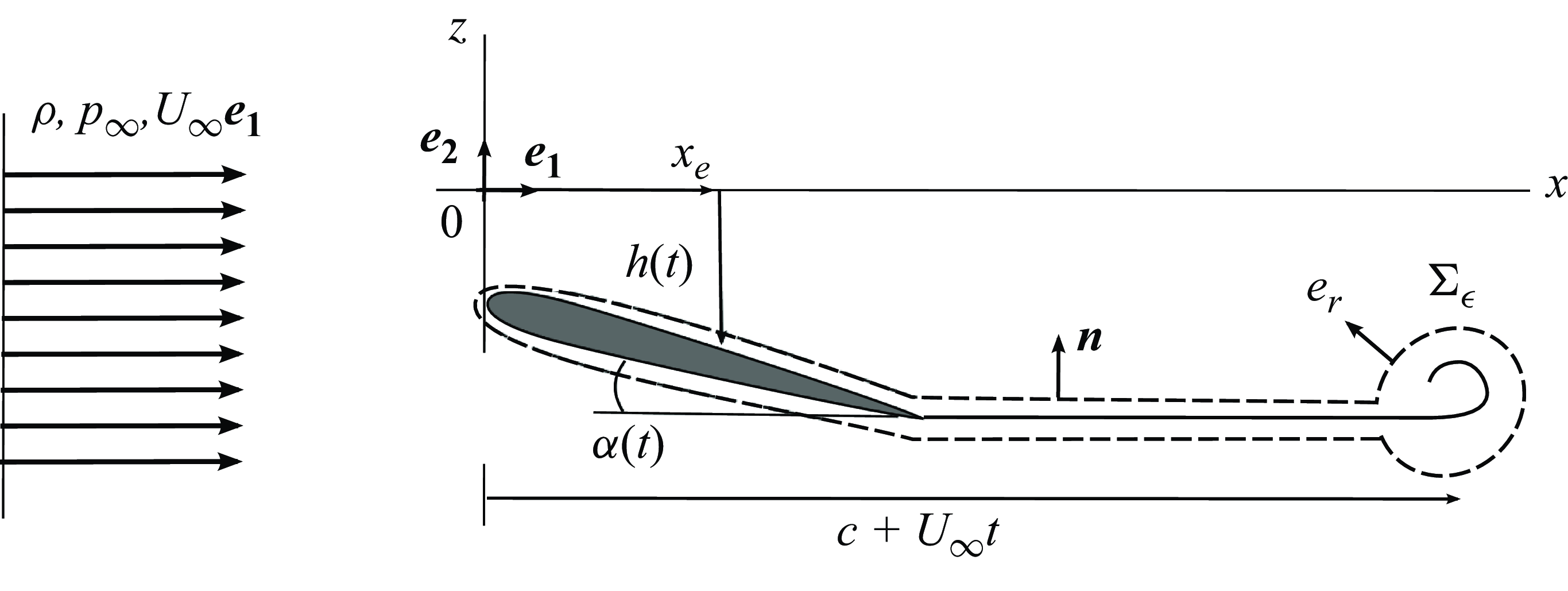
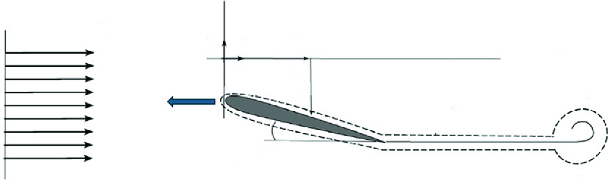
Figure 1. Sketch of the canonical flow considered in this study.
The canonical flow to be studied in what follows, which employs the same notation and sign conventions as those used in Bisplinghoff, Ashley & Halfman (Reference Bisplinghoff, Ashley and Halfman1996) except for the fact that, here, the origin of the Cartesian coordinate system is located at the leading edge of the airfoil, is illustrated figure 1: an airfoil of chord $c$
extending along
$c$
extending along $0 \leqslant x\leqslant c$
, with
$0 \leqslant x\leqslant c$
, with $x$
and
$x$
and $z$
denoting the Cartesian horizontal and vertical coordinates with associated unit vectors
$z$
denoting the Cartesian horizontal and vertical coordinates with associated unit vectors $\boldsymbol{e_1}$
and
$\boldsymbol{e_1}$
and $\boldsymbol{e_2}$
, forms a time-dependent angle of attack
$\boldsymbol{e_2}$
, forms a time-dependent angle of attack $\alpha (t)$
with an incident uniform stream of density
$\alpha (t)$
with an incident uniform stream of density $\rho$
and velocity
$\rho$
and velocity $\boldsymbol{v}=U_\infty \boldsymbol{e_1}$
. The origin of times is set at
$\boldsymbol{v}=U_\infty \boldsymbol{e_1}$
. The origin of times is set at $t=0$
and, hence, within the classical linearised potential flow approach, the horizontal position of the starting vortex is
$t=0$
and, hence, within the classical linearised potential flow approach, the horizontal position of the starting vortex is $x=c + U_\infty t$
(Wagner Reference Wagner1925; Theodorsen Reference Theodorsen1935; von Kármán & Sears Reference von Kármán and Sears1938; Glauert Reference Glauert1983; Ashley & Landahl Reference Ashley and Landahl1985). Moreover, the vertical position of the point located at a distance
$x=c + U_\infty t$
(Wagner Reference Wagner1925; Theodorsen Reference Theodorsen1935; von Kármán & Sears Reference von Kármán and Sears1938; Glauert Reference Glauert1983; Ashley & Landahl Reference Ashley and Landahl1985). Moreover, the vertical position of the point located at a distance $x=x_e\lt c$
from the leading edge of the airfoil is
$x=x_e\lt c$
from the leading edge of the airfoil is $z_a(x_e,t)=-h(t)$
and, hence, for the case of a symmetrical airfoil with zero thickness considered, here,
$z_a(x_e,t)=-h(t)$
and, hence, for the case of a symmetrical airfoil with zero thickness considered, here,
 \begin{equation} z_a(x,t)=-h(t)-\alpha (t)\left (x-x_e\right ) , \end{equation}
with the subscripts a and w referring from now on to quantities corresponding to either the airfoil or the wake. Notice that, in this contribution, positive lift $\ell (t)$
corresponds to a force in the positive
$\ell (t)$
corresponds to a force in the positive $z$
-direction, positive thrust
$z$
-direction, positive thrust $-d(t)$
is positive in the negative
$-d(t)$
is positive in the negative $x$
-direction, whereas positive
$x$
-direction, whereas positive $h(t)$
corresponds to motion in the negative
$h(t)$
corresponds to motion in the negative $z$
-direction and, similarly, positive torque
$z$
-direction and, similarly, positive torque $m(t)$
is in the counterclockwise direction, while positive
$m(t)$
is in the counterclockwise direction, while positive $\alpha (t)$
gives clockwise rotation. The aerodynamic force
$\alpha (t)$
gives clockwise rotation. The aerodynamic force $\boldsymbol{f}(t)=\ell (t)\boldsymbol{e_2} + d(t)\boldsymbol{e_1}$
and torque over such an airfoil, which possesses the two degrees of freedom
$\boldsymbol{f}(t)=\ell (t)\boldsymbol{e_2} + d(t)\boldsymbol{e_1}$
and torque over such an airfoil, which possesses the two degrees of freedom $\alpha (t)$
and
$\alpha (t)$
and $h(t)$
, are calculated for the common case in which the Reynolds number verifies the condition
$h(t)$
, are calculated for the common case in which the Reynolds number verifies the condition $Re=\rho U_\infty c/\mu \gg 1$
, with
$Re=\rho U_\infty c/\mu \gg 1$
, with $\mu$
indicating the dynamic viscosity; moreover, we will consider that the relative density variations are negligible and that
$\mu$
indicating the dynamic viscosity; moreover, we will consider that the relative density variations are negligible and that $\alpha (t)\ll 1$
,
$\alpha (t)\ll 1$
, $z_{a,w}/c\ll 1$
,
$z_{a,w}/c\ll 1$
, $h/c\ll 1$
, with the vertical positions of the points on the airfoil
$h/c\ll 1$
, with the vertical positions of the points on the airfoil $z_a(x,t)$
defined in (2.1) and
$z_a(x,t)$
defined in (2.1) and $z_w(x,t)$
referring to the vertical position of the points in the wake. Therefore, under these conditions, the thin boundary layer of thickness
$z_w(x,t)$
referring to the vertical position of the points in the wake. Therefore, under these conditions, the thin boundary layer of thickness $\delta$
such that
$\delta$
such that $\delta /c\propto Re^{-1/2}\ll 1$
does not separate and, hence, the classical, linearised potential flow theory summarised in e.g. Ashley & Landahl (Reference Ashley and Landahl1985), is applicable.
$\delta /c\propto Re^{-1/2}\ll 1$
does not separate and, hence, the classical, linearised potential flow theory summarised in e.g. Ashley & Landahl (Reference Ashley and Landahl1985), is applicable.
Indeed, outside the thin boundary layer and the wake, the velocity field is irrotational, namely, $\boldsymbol{v}=\nabla \phi$
, with
$\boldsymbol{v}=\nabla \phi$
, with $\phi =U_\infty x + \phi '$
and
$\phi =U_\infty x + \phi '$
and $\phi '$
indicating the perturbed velocity potential associated with the perturbed velocity field
$\phi '$
indicating the perturbed velocity potential associated with the perturbed velocity field $\boldsymbol{v}^{\prime}=\nabla \phi '=u'\boldsymbol{e_1} + w'\boldsymbol{e_2}$
verifying the condition
$\boldsymbol{v}^{\prime}=\nabla \phi '=u'\boldsymbol{e_1} + w'\boldsymbol{e_2}$
verifying the condition $|\nabla \phi '|/U_\infty \ll 1$
except, as will become clear in what follows, at the leading edge,
$|\nabla \phi '|/U_\infty \ll 1$
except, as will become clear in what follows, at the leading edge, $x\rightarrow 0$
and, for the case of an airfoil which is suddenly set into motion, at
$x\rightarrow 0$
and, for the case of an airfoil which is suddenly set into motion, at $x\rightarrow c + U_\infty t$
i.e. where the starting vortex is located. Then, by virtue of the continuity equation
$x\rightarrow c + U_\infty t$
i.e. where the starting vortex is located. Then, by virtue of the continuity equation $\nabla \cdot \boldsymbol{v}=0$
, the perturbed potential satisfies the Laplace equation
$\nabla \cdot \boldsymbol{v}=0$
, the perturbed potential satisfies the Laplace equation
 \begin{equation} \nabla ^2\phi '=0 , \end{equation}
which must be solved subject to the boundary condition at infinity $\phi '\rightarrow 0$
and to the linearised impenetrability condition, which can be expressed as
$\phi '\rightarrow 0$
and to the linearised impenetrability condition, which can be expressed as
 \begin{equation} \frac {{\rm D}F}{{\rm D}t}=\frac {\partial F}{\partial t} + \left (U_\infty \boldsymbol{e_1} + \nabla \phi '\right )\cdot \nabla F=0\quad \mathrm{with}\quad F=z-z_{a,w}(x,t), \end{equation}
and with $z_a(x,t)$
given in (2.1).
$z_a(x,t)$
given in (2.1).
The standard linearisation of (2.3) yields (Ashley & Landahl Reference Ashley and Landahl1985)
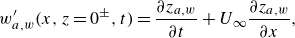 \begin{equation} w'_{a,w}(x,z=0^\pm ,t)=\frac {\partial z_{a,w}}{\partial t} + U_\infty \frac {\partial z_{a,w}}{\partial x} ,\end{equation}
with $z=0^{\pm }$
indicating the upper and lower sides of the airfoil and the wake and
$z=0^{\pm }$
indicating the upper and lower sides of the airfoil and the wake and $w'_{a,w}$
referring to the vertical component of the velocity on the airfoil or at the wake. In view of the linearised impenetrability boundary condition at
$w'_{a,w}$
referring to the vertical component of the velocity on the airfoil or at the wake. In view of the linearised impenetrability boundary condition at $0\leqslant x\leqslant c$
given by (2.1) and (2.4), we seek antisymmetric solutions of the Laplace equation (2.2) in the form of a vortex sheet extending along the airfoil and the wake, whose circulation density is the one satisfying the condition expressed by (2.1) and (2.4). Notice that, making use of the notation
$0\leqslant x\leqslant c$
given by (2.1) and (2.4), we seek antisymmetric solutions of the Laplace equation (2.2) in the form of a vortex sheet extending along the airfoil and the wake, whose circulation density is the one satisfying the condition expressed by (2.1) and (2.4). Notice that, making use of the notation $\phi ^{\prime \pm }=\phi '(x,z=0^\pm ,t)$
,
$\phi ^{\prime \pm }=\phi '(x,z=0^\pm ,t)$
, $\Gamma (x,t)=\oint _C (U_\infty \boldsymbol{e_1} + \nabla \phi ' )\cdot {\rm d}\boldsymbol{\ell }= (\phi ^ + -\phi ^{-} )=2\phi ^ + (x,t)$
and
$\Gamma (x,t)=\oint _C (U_\infty \boldsymbol{e_1} + \nabla \phi ' )\cdot {\rm d}\boldsymbol{\ell }= (\phi ^ + -\phi ^{-} )=2\phi ^ + (x,t)$
and $\gamma (x,t)=u^{\prime + }-u^{\prime -}=\partial \Gamma /\partial x$
, in this contribution
$\gamma (x,t)=u^{\prime + }-u^{\prime -}=\partial \Gamma /\partial x$
, in this contribution
 \begin{equation} \Gamma (x\gt 0,t)=2\phi ^ + (x\gt 0,t)=\int _{-\infty }^x\gamma (x_0,t)\,{\rm d}x_0=\int _0^x \gamma (x_0,t) {\rm d}x_0 \end{equation}
refers to the clockwise circulation along any closed loop encircling the leading edge of the airfoil and connecting the points $(x\gt 0,z=0^{-})$
and
$(x\gt 0,z=0^{-})$
and $(x\gt 0,z=0^ + )$
, whereas
$(x\gt 0,z=0^ + )$
, whereas $\gamma (x,t)$
indicates the circulation density. In (2.5) we have taken into account that, since the origin of the vortex sheet is the leading edge of the airfoil, which is located at
$\gamma (x,t)$
indicates the circulation density. In (2.5) we have taken into account that, since the origin of the vortex sheet is the leading edge of the airfoil, which is located at $x=0$
,
$x=0$
, $\gamma (x\lt 0,t)=0$
, and hence the circulation for
$\gamma (x\lt 0,t)=0$
, and hence the circulation for $x\lt 0$
is also zero because
$x\lt 0$
is also zero because $\Gamma (x\lt 0,t)=\int _{-\infty }^x \gamma (x_0,t)\,{\rm d}x_0=0$
. In the following,
$\Gamma (x\lt 0,t)=\int _{-\infty }^x \gamma (x_0,t)\,{\rm d}x_0=0$
. In the following, $\Gamma _{a,w}(x,t)$
and
$\Gamma _{a,w}(x,t)$
and $\gamma _{a,w}(x,t)$
will indicate the values of the circulation and of the circulation density on the airfoil, which extends along
$\gamma _{a,w}(x,t)$
will indicate the values of the circulation and of the circulation density on the airfoil, which extends along $0\leqslant x\leqslant c$
or at the wake, which extends along
$0\leqslant x\leqslant c$
or at the wake, which extends along $x\gt c$
.
$x\gt c$
.
The equation governing the pressure jump at $z=0$
, namely,
$z=0$
, namely, $\Delta p(x,z=0,t)=p'(x,z=0^{-},t)-p'(x,z=0^{ + },t)=p^{\prime -}(x,t)-p^{\prime + }(x,t)$
, with
$\Delta p(x,z=0,t)=p'(x,z=0^{-},t)-p'(x,z=0^{ + },t)=p^{\prime -}(x,t)-p^{\prime + }(x,t)$
, with $p'=p-p_\infty$
indicating the perturbed pressure, can be deduced from the linearised Bernoulli equation particularised at
$p'=p-p_\infty$
indicating the perturbed pressure, can be deduced from the linearised Bernoulli equation particularised at $z=0^\pm$
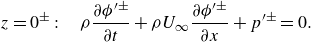 \begin{align} & z=0^{\pm }:\quad \rho \frac {\partial \phi ^{\prime \pm }}{\partial t} + \rho U_\infty \frac {\partial \phi ^{\prime \pm }}{\partial x} + p^{\prime \pm }=0 . \end{align}
Hence, the subtraction of the two equations in (2.6) yields
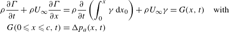 \begin{align} \rho \frac {\partial \Gamma }{\partial t} + \rho U_\infty \frac {\partial \Gamma }{\partial x} & = \rho \frac {\partial }{\partial t}\left (\int _0^x\gamma \,{\rm d}x_0\right ) + \rho U_\infty \gamma =G(x,t) \quad \mathrm{with} \nonumber \\ G(0\leqslant x\leqslant c,t) & = \Delta p_a(x,t) \end{align}
with $\Delta p_a$
the pressure jump at the airfoil and, since
$\Delta p_a$
the pressure jump at the airfoil and, since $\Delta p=0$
for
$\Delta p=0$
for $x\lt 0$
and
$x\lt 0$
and $x\gt c$
, we conclude that
$x\gt c$
, we conclude that $ G(x\lt 0,t)=G(x\gt c,t)=0$
in (2.7), a fact implying that the material derivatives of both
$ G(x\lt 0,t)=G(x\gt c,t)=0$
in (2.7), a fact implying that the material derivatives of both $\Gamma$
and
$\Gamma$
and $\gamma$
are zero at
$\gamma$
are zero at $z=0$
for
$z=0$
for $x\lt 0$
and
$x\lt 0$
and $x\gt c$
, namely (Ashley & Landahl Reference Ashley and Landahl1985),
$x\gt c$
, namely (Ashley & Landahl Reference Ashley and Landahl1985),
 \begin{equation} \frac {{\rm D}\Gamma }{{\rm D}t}=\frac {\partial }{\partial x} \! \left (\frac {{\rm D}\Gamma }{{\rm D}t}\right )=0\Rightarrow \frac {\partial \Gamma }{\partial t} + U_\infty \gamma =0 ,\quad \frac {\partial \gamma }{\partial t} + U_\infty \frac {\partial \gamma }{\partial x}=0 \quad \mathrm{for}\quad x\lt 0 , \quad x\gt c . \end{equation}
Taking into account that $\Gamma =0$
for
$\Gamma =0$
for $x\rightarrow -\infty$
and also for instants
$x\rightarrow -\infty$
and also for instants $t\lt 0$
and that the circulation at the origin of the wake is prescribed by the circulation around the airfoil, namely,
$t\lt 0$
and that the circulation at the origin of the wake is prescribed by the circulation around the airfoil, namely,
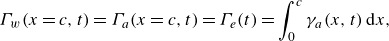 \begin{equation} \Gamma _w(x=c,t)=\Gamma _a(x=c,t)=\Gamma _e(t)=\int _0^c \gamma _a(x,t)\,{\rm d}x , \end{equation}
with $\Gamma _e(t)$
the circulation around the airfoil, we deduce from (2.8) and (2.9) that
$\Gamma _e(t)$
the circulation around the airfoil, we deduce from (2.8) and (2.9) that
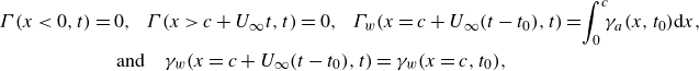 \begin{align} &\Gamma (x\lt 0,t)=0 ,\!\!\quad \Gamma (x\gt c + U_\infty t,t)=0 ,\!\!\quad \Gamma _w(x=c + U_\infty (t-t_0),t)=\!\int _0^c \!\!\gamma _a(x,t_0){\rm d}x ,\notag\\&\qquad\qquad\qquad \mathrm{and}\quad \gamma _w(x=c + U_\infty (t-t_0),t)=\gamma _w(x=c,t_0) , \end{align}
with $\gamma _w(x\rightarrow c,t_0)$
given by (2.8) and (2.10) – see also equations (13)–(27) in Ashley & Landahl (Reference Ashley and Landahl1985)
$\gamma _w(x\rightarrow c,t_0)$
given by (2.8) and (2.10) – see also equations (13)–(27) in Ashley & Landahl (Reference Ashley and Landahl1985)
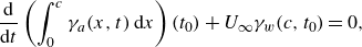 \begin{align} \frac {\rm d}{{\rm d} t}\left (\int _0^c\gamma _a(x,t)\,{\rm d}x\right )(t_0) + U_\infty \gamma _w(c,t_0)=0 , \end{align}
where $\gamma _w(x\rightarrow c,t_0)=\gamma _w(c,t_0)$
from which we conclude that
$\gamma _w(x\rightarrow c,t_0)=\gamma _w(c,t_0)$
from which we conclude that
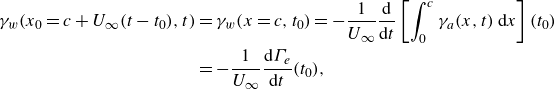 \begin{align} \gamma _w(x_0=c + U_\infty (t-t_0),t)&=\gamma _w(x=c,t_0)=-\frac {1}{U_\infty }\frac {\rm d}{{\rm d}t}\left [\int _0^c \gamma _a(x,t)\,{\rm d}x\right ](t_0)\notag\\&=-\frac {1}{U_\infty }\frac {{\rm d}\Gamma _e}{{\rm d}t}(t_0) , \end{align}
with the circulation around the airfoil $\Gamma _e(t)$
defined in (2.9). Equations (2.7) and (2.12) indicate that the unsteady lift force and the torque
$\Gamma _e(t)$
defined in (2.9). Equations (2.7) and (2.12) indicate that the unsteady lift force and the torque
 \begin{equation} \ell (t)=\int _0^c\Delta p_a(x,t)\,{\rm d}x\quad \mathrm{and}\quad m(t)=\int _0^c x\,\Delta p_a(x,t)\,{\rm d}x , \end{equation}
as well as the density of circulation along the wake, $\gamma _w(x,t)$
, can be expressed as a function of
$\gamma _w(x,t)$
, can be expressed as a function of $\gamma _a(x,t)$
.
$\gamma _a(x,t)$
.
Finally, the density of circulation at the airfoil, $\gamma _a(x,t)$
, is deduced by imposing that the perturbed vertical velocity induced by the vortex sheet extending along
$\gamma _a(x,t)$
, is deduced by imposing that the perturbed vertical velocity induced by the vortex sheet extending along $z=0$
,
$z=0$
, $0\leqslant x\leqslant c + U_\infty t$
satisfies the linearised impenetrability condition given by (2.1) and (2.4), namely (Ashley & Landahl Reference Ashley and Landahl1985),
$0\leqslant x\leqslant c + U_\infty t$
satisfies the linearised impenetrability condition given by (2.1) and (2.4), namely (Ashley & Landahl Reference Ashley and Landahl1985),
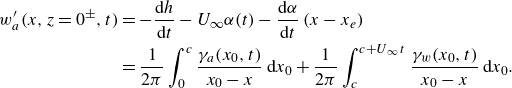 \begin{align} w'_a(x,z=0^\pm ,t)&=-\frac {{\rm d}h}{{\rm d}t}-U_\infty \alpha (t)-\frac {{\rm d}\alpha }{{\rm d}t}\left (x-x_e\right )\notag \\&=\frac {1}{2\pi }\int _0^{c}\frac {\gamma _a(x_0,t)}{x_0-x}\,{\rm d}x_0 + \frac {1}{2\pi }\int _c^{c + U_\infty \,t}\frac {\gamma _w(x_0,t)}{x_0-x}\,{\rm d}x_0 . \end{align}
Introducing the change of variables
 \begin{equation} x_0=c + U_\infty \left (t-t_0\right )\Rightarrow {\rm d}x_0=-U_\infty {\rm d}t_0, \end{equation}
and taking into account that the second integral at the right-hand side of (2.14) can be expressed solely in terms of $\gamma _a$
by means of (2.12), the equation for
$\gamma _a$
by means of (2.12), the equation for $\gamma _{a}(x,t)$
reads
$\gamma _{a}(x,t)$
reads
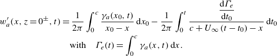 \begin{align} w'_a(x,z=0^\pm ,t)&=\frac {1}{2\pi }\int _0^{c}\frac {\gamma _a(x_0,t)}{x_0-x}\,{\rm d}x_0-\frac {1}{2\pi }\int _0^{t}\frac {\dfrac{{\rm d}\Gamma _e}{{\rm d}t_0}}{c + U_\infty \left (t-t_0\right )-x}\,{\rm d}t_0 \notag\\ &\quad \mathrm{with} \quad \Gamma _e(t)=\int _0^c\gamma _a(x,t)\,{\rm d}x . \end{align}
In order to solve the integral equation (2.16) notice first that, since $\Gamma (x\rightarrow -\infty ,t)=0$
then, by virtue of (2.8),
$\Gamma (x\rightarrow -\infty ,t)=0$
then, by virtue of (2.8), $\Gamma (x\lt 0,t)=0$
and hence,
$\Gamma (x\lt 0,t)=0$
and hence, $\phi '(z=0^{\pm },x\lt 0)=0$
. Consequently, the local solution of the Laplace equation (2.2) at the leading edge of the airfoil is the one corresponding to the flow around a wedge of angle
$\phi '(z=0^{\pm },x\lt 0)=0$
. Consequently, the local solution of the Laplace equation (2.2) at the leading edge of the airfoil is the one corresponding to the flow around a wedge of angle $2\pi$
, namely,
$2\pi$
, namely,
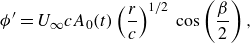 \begin{equation} \phi '=U_\infty c A_0(t)\left (\frac{r}{c}\right )^{1/2}\,\cos \left (\frac{\beta}{2}\right ) , \end{equation}
with $A_0(t)$
a dimensionless time-dependent constant,
$A_0(t)$
a dimensionless time-dependent constant, $r/c\ll 1$
the radial distance to the leading edge – which is located at
$r/c\ll 1$
the radial distance to the leading edge – which is located at $z=0$
,
$z=0$
, $x=0$
in the linearised theory – and
$x=0$
in the linearised theory – and $0\leqslant \beta \leqslant 2\pi$
indicating the polar angle measured in counterclockwise manner from the horizontal axis.
$0\leqslant \beta \leqslant 2\pi$
indicating the polar angle measured in counterclockwise manner from the horizontal axis.
Taking into account: (i) that the Kutta condition ensures that $\gamma _a(x=c,t)$
is finite in order to avoid that the flow turns around the trailing edge of the airfoil and (ii) that
$\gamma _a(x=c,t)$
is finite in order to avoid that the flow turns around the trailing edge of the airfoil and (ii) that $\gamma _a(x/c\ll 1,t)$
is given by
$\gamma _a(x/c\ll 1,t)$
is given by
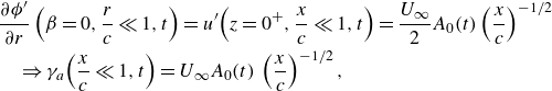 \begin{align} &\frac {\partial \phi '}{\partial r} \left(\beta =0,\frac{r}{c}\ll 1,t \right)=u'\!\left(z=0^ + ,\frac{x}{c}\ll 1,t \right)=\frac {U_\infty }{2} A_0(t) \left (\frac{x}{c}\right )^{-1/2}\notag\\&\quad \Rightarrow \gamma _a \!\left (\frac{x}{c}\ll 1,t \right)=U_\infty A_0(t)\,\left (\frac{x}{c}\right )^{-1/2} , \end{align}
where use of (2.17) has been made, it can be concluded that the integral equation (2.16) can be solved using Glauert’s method, which relies on expressing the unknown function $\gamma _a(x,t)$
as the infinite series (Glauert Reference Glauert1983)
$\gamma _a(x,t)$
as the infinite series (Glauert Reference Glauert1983)
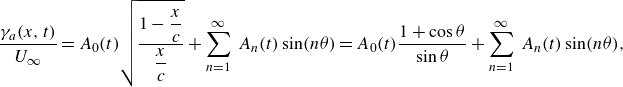 \begin{align} &\frac {\gamma _a(x,t)}{U_\infty }=A_0(t)\sqrt {\frac {1- \dfrac{x}{c}}{\dfrac{x}{c}}} + \sum _{n=1}^{\infty }\,A_n(t)\sin (n\theta )=A_0(t)\frac {1 + \cos \theta }{\sin \theta } + \sum _{n=1}^{\infty }\,A_n(t)\sin (n\theta ) , \end{align}
where we have introduced the change of variables
 \begin{equation} \frac {x}{c}=\frac {1-\cos \theta }{2} ,\end{equation}
and, therefore, $\theta =0$
at
$\theta =0$
at $x=0$
and
$x=0$
and $\theta =\pi$
at
$\theta =\pi$
at $x=c$
. Notice that the expansion (2.19) implies that
$x=c$
. Notice that the expansion (2.19) implies that $\gamma _a(x=c,t)=0$
and, hence, the density of circulation at
$\gamma _a(x=c,t)=0$
and, hence, the density of circulation at $x=c$
does not satisfy the physical condition
$x=c$
does not satisfy the physical condition $\gamma _a(x=c,t)=\gamma _w(x=c,t)$
. However, the continuity of the circulation density at the trailing edge could be enforced following the procedure detailed in Alben (Reference Alben2010) and Eldredge (Reference Eldredge2019) and references therein by analytically removing the logarithmic singularity at
$\gamma _a(x=c,t)=\gamma _w(x=c,t)$
. However, the continuity of the circulation density at the trailing edge could be enforced following the procedure detailed in Alben (Reference Alben2010) and Eldredge (Reference Eldredge2019) and references therein by analytically removing the logarithmic singularity at $x=c$
in (2.16). This more elaborate method provides a faster convergence to the solution which, however, can also be found using the more classical procedure followed here by simply retaining a larger number of terms in (2.19), see Alben (Reference Alben2010).
$x=c$
in (2.16). This more elaborate method provides a faster convergence to the solution which, however, can also be found using the more classical procedure followed here by simply retaining a larger number of terms in (2.19), see Alben (Reference Alben2010).
Then, the substitution of the expansion (2.19) into the integral equation (2.16) provides us with the values of the time-dependent coefficients $A_i(t)$
as a function of
$A_i(t)$
as a function of $\alpha (t)$
and
$\alpha (t)$
and $h(t)$
, as detailed in the Supplementary Material, see also Wagner (Reference Wagner1925), Theodorsen (Reference Theodorsen1935), von Kármán & Sears (Reference von Kármán and Sears1938), Wu (Reference Wu1961) and references therein. Once the values of
$h(t)$
, as detailed in the Supplementary Material, see also Wagner (Reference Wagner1925), Theodorsen (Reference Theodorsen1935), von Kármán & Sears (Reference von Kármán and Sears1938), Wu (Reference Wu1961) and references therein. Once the values of $A_i(t)$
are known,
$A_i(t)$
are known, $\Delta p_a$
,
$\Delta p_a$
, $\ell (t)$
and
$\ell (t)$
and $m(t)$
can be determined by means of (2.7) and (2.13), as illustrated, for instance, in the Supplementary Material. Now that
$m(t)$
can be determined by means of (2.7) and (2.13), as illustrated, for instance, in the Supplementary Material. Now that $\ell (t)$
is known, the value of the drag force can be obtained by adding to the projection in the flight direction of the lift force the resulting suction force at the leading edge of the airfoil, yielding
$\ell (t)$
is known, the value of the drag force can be obtained by adding to the projection in the flight direction of the lift force the resulting suction force at the leading edge of the airfoil, yielding
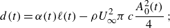 \begin{equation} d(t)=\alpha (t)\ell (t)-\rho U^2_\infty \pi \,c \frac {A^2_0(t)}{4}\, ; \end{equation}
see Garrick (Reference Garrick1936), Wu (Reference Wu1961) and references therein, as well as the next subsection. Hence, the thrust force obtained by the direct integration of the pressure distribution around the airfoil is given by
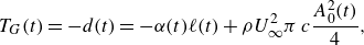 \begin{equation} T_G(t)=-d(t)=-\alpha (t)\ell (t) + \rho U^2_\infty \pi \,c \frac {A^2_0(t)}{4} ,\end{equation}
where we have made use of (2.21) and the subscript $G$
indicates Garrick. Let us point out here that the expression of
$G$
indicates Garrick. Let us point out here that the expression of $A_0(t)$
in (2.22) for the case of periodic oscillations of the airfoil was provided by Garrick (Reference Garrick1936) using the results of Theodorsen (Reference Theodorsen1935), whereas the corresponding value for arbitrary heaving or pitching motions is deduced elsewhere; see, for instance, the Supplementary Material.
$A_0(t)$
in (2.22) for the case of periodic oscillations of the airfoil was provided by Garrick (Reference Garrick1936) using the results of Theodorsen (Reference Theodorsen1935), whereas the corresponding value for arbitrary heaving or pitching motions is deduced elsewhere; see, for instance, the Supplementary Material.
2.1. Forces calculated through a momentum balance
So far we have calculated the unsteady lift and thrust forces on the airfoil as a result of the integration of the pressure distribution around the solid. It is now our purpose to calculate the aerodynamic force $\boldsymbol{f}$
through a momentum balance using the control volume
$\boldsymbol{f}$
through a momentum balance using the control volume $\Omega _c(t)$
limited by a fixed surface
$\Omega _c(t)$
limited by a fixed surface $\Sigma _\infty$
of dimensionless radius
$\Sigma _\infty$
of dimensionless radius $R/c\rightarrow \infty$
which encircles both the solid and the wake, by the surface
$R/c\rightarrow \infty$
which encircles both the solid and the wake, by the surface $\Sigma _{a,w}$
bounding both the solid and the wake and by
$\Sigma _{a,w}$
bounding both the solid and the wake and by $\Sigma _\epsilon$
, which is a circle of radius
$\Sigma _\epsilon$
, which is a circle of radius $\epsilon \rightarrow 0$
centred where the starting vortex is located, namely, at
$\epsilon \rightarrow 0$
centred where the starting vortex is located, namely, at $x=c + U_\infty t$
. The momentum balance applied at the control volume
$x=c + U_\infty t$
. The momentum balance applied at the control volume $\Omega _c(t)$
defined above yields
$\Omega _c(t)$
defined above yields
 \begin{equation} \frac {\rm d}{{\rm d}t}\int _{\Omega _c(t)} \rho \boldsymbol{v} {\rm d}\omega + \int _{\partial \Omega _c} \rho \boldsymbol{v}\left (\boldsymbol{v}-\boldsymbol{v_c}\right )\cdot \boldsymbol{n_c}\,{\rm d}\sigma =\int _{\partial \Omega _c} \left (p-p_\infty \right ) \left (-\boldsymbol{n_c}\right )\,{\rm d}\sigma , \end{equation}
with $\boldsymbol{n_c}$
the unit normal pointing outwards the control volume,
$\boldsymbol{n_c}$
the unit normal pointing outwards the control volume, $\boldsymbol{v}=\nabla \phi$
and
$\boldsymbol{v}=\nabla \phi$
and $\boldsymbol{v_c}$
indicating the velocity of the surfaces bounding the control volume, namely,
$\boldsymbol{v_c}$
indicating the velocity of the surfaces bounding the control volume, namely, $\boldsymbol{v_c}=U_\infty \boldsymbol{e_1}$
at
$\boldsymbol{v_c}=U_\infty \boldsymbol{e_1}$
at $\Sigma _\epsilon$
and
$\Sigma _\epsilon$
and $ (\boldsymbol{v}-\boldsymbol{v_c} )\boldsymbol{\cdot} \boldsymbol{n_c}=0$
at
$ (\boldsymbol{v}-\boldsymbol{v_c} )\boldsymbol{\cdot} \boldsymbol{n_c}=0$
at $\Sigma _{a,w}$
. Since there is no relative momentum flux across the surfaces
$\Sigma _{a,w}$
. Since there is no relative momentum flux across the surfaces $\Sigma _{a,w}$
, and taking into account that the pressure force at the airfoil is
$\Sigma _{a,w}$
, and taking into account that the pressure force at the airfoil is
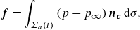 \begin{equation} \boldsymbol{f}=\int _{\Sigma _a(t)} \left (p-p_\infty \right ) \boldsymbol{n_c}\,{\rm d}\sigma , \end{equation}
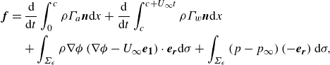
(2.23) can be written, making use of Gauss’ theorem, as
 \begin{align} &\boldsymbol{f}=-\frac {\rm d}{{\rm d}t}\!\int _{\Sigma _a\bigcup \Sigma _w} \rho \phi \boldsymbol{n_c}\, {\rm d}\sigma + \!\int _{\Sigma _\epsilon } \rho \nabla \phi \left (\nabla \phi -U_\infty \boldsymbol{e_1}\right )\cdot \boldsymbol{e_r}{\rm d}\sigma + \!\int _{\Sigma _\epsilon } \left (p-p_\infty \right ) \left (-\boldsymbol{e_r}\right ) {\rm d}\sigma , \end{align}
where we have taken into account that $\boldsymbol{v}=\nabla \phi =\nabla \phi ' + U_\infty \,\boldsymbol{e_1}$
and
$\boldsymbol{v}=\nabla \phi =\nabla \phi ' + U_\infty \,\boldsymbol{e_1}$
and $\boldsymbol{e_r}$
refers to the unit vector in polar coordinates, see figure 1. Moreover, in (2.25) we have made use of the fact that the integrals evaluated at
$\boldsymbol{e_r}$
refers to the unit vector in polar coordinates, see figure 1. Moreover, in (2.25) we have made use of the fact that the integrals evaluated at $\Sigma _\infty$
tend to zero because of the Bernoulli equation
$\Sigma _\infty$
tend to zero because of the Bernoulli equation $\rho \partial \phi /\partial t + \rho |\nabla \phi |^2/2 + p=K$
and because
$\rho \partial \phi /\partial t + \rho |\nabla \phi |^2/2 + p=K$
and because $\Sigma _\infty$
encircles both the airfoil and the wake and, hence, the circulation around
$\Sigma _\infty$
encircles both the airfoil and the wake and, hence, the circulation around $\Sigma _\infty$
is zero, which implies that the perturbed velocity field decays faster than
$\Sigma _\infty$
is zero, which implies that the perturbed velocity field decays faster than $U_\infty c/R$
at infinity, which ensures that both the flux of momentum and the integral of
$U_\infty c/R$
at infinity, which ensures that both the flux of momentum and the integral of $|\nabla \phi |^2$
along
$|\nabla \phi |^2$
along $\Sigma _\infty$
tend to zero. Then, the aerodynamic force can be written, in the linearised approach, as
$\Sigma _\infty$
tend to zero. Then, the aerodynamic force can be written, in the linearised approach, as
 \begin{align} \boldsymbol{f}&=\frac {\rm d}{{\rm d}t}\int _0^c \rho \Gamma _a \boldsymbol{n} {\rm d}x + \frac {\rm d}{{\rm d}t}\int _c^{c + U_\infty t} \rho \Gamma _w \boldsymbol{n} {\rm d}x \notag\\&\quad + \int _{\Sigma _\epsilon } \rho \nabla \phi \left (\nabla \phi -U_\infty \boldsymbol{e_1}\right )\cdot \boldsymbol{e_r}{\rm d}\sigma + \int _{\Sigma _\epsilon } \left (p-p_\infty \right ) \left (-\boldsymbol{e_r}\right ) {\rm d}\sigma , \end{align}
with $\boldsymbol{n}$
the unit vector pointing outwards the side
$\boldsymbol{n}$
the unit vector pointing outwards the side $z=0^ + $
of
$z=0^ + $
of $\Sigma _a$
and
$\Sigma _a$
and $\Sigma _w$
, see figure 1, and where we have taken into account that the unit normal pointing outwards the side
$\Sigma _w$
, see figure 1, and where we have taken into account that the unit normal pointing outwards the side $z=0^-$
of
$z=0^-$
of $\Sigma _a$
and
$\Sigma _a$
and $\Sigma _w$
is
$\Sigma _w$
is $-\boldsymbol{n}$
, this being the reason why the integrand in the first two integrals in (2.26) is
$-\boldsymbol{n}$
, this being the reason why the integrand in the first two integrals in (2.26) is $\Gamma =\phi '^ + -\phi '^-$
; in addition, in (2.26) we have made use of the fact that, by virtue of (2.17) and of the paragraph preceding this equation, where it is shown that
$\Gamma =\phi '^ + -\phi '^-$
; in addition, in (2.26) we have made use of the fact that, by virtue of (2.17) and of the paragraph preceding this equation, where it is shown that $\Gamma (x\leqslant 0,t)=0$
, the value of the integral extending along a small region near the leading edge tends to zero. Finally, since
$\Gamma (x\leqslant 0,t)=0$
, the value of the integral extending along a small region near the leading edge tends to zero. Finally, since $\Gamma (x\gt c + U_\infty t,t)=0$
, see (2.10), the leading-order equation for the perturbed potential at
$\Gamma (x\gt c + U_\infty t,t)=0$
, see (2.10), the leading-order equation for the perturbed potential at $\Sigma _\epsilon$
, corresponds to the one characterising the flow around a wedge of angle
$\Sigma _\epsilon$
, corresponds to the one characterising the flow around a wedge of angle $-\pi \leqslant \beta \leqslant \pi$
, namely,
$-\pi \leqslant \beta \leqslant \pi$
, namely,
 \begin{align} &\phi '=U_\infty c C \sin \!\left(\frac{\beta}{2} \right)\left (\frac {r}{c}\right )^{1/2}\notag \\&\quad\Rightarrow \nabla \phi '=\frac {C}{2} U_\infty \sin \! \left(\frac{\beta}{2} \right) \left (\frac {r}{c}\right )^{-1/2}\boldsymbol{e_r} + \frac {C}{2} U_\infty \cos \!\left (\frac{\beta}{2} \right) \left (\frac {r}{c}\right )^{-1/2}\boldsymbol{e_\beta } , \end{align}
with $\boldsymbol{e_r}=\cos \beta \boldsymbol{e_1} + \sin \beta \boldsymbol{e_2}$
,
$\boldsymbol{e_r}=\cos \beta \boldsymbol{e_1} + \sin \beta \boldsymbol{e_2}$
, $\boldsymbol{e_\beta }=-\sin \beta \boldsymbol{e_1} + \cos \beta \boldsymbol{e_2}$
,
$\boldsymbol{e_\beta }=-\sin \beta \boldsymbol{e_1} + \cos \beta \boldsymbol{e_2}$
, $r/c$
indicating the dimensionless distance to the starting vortex located at
$r/c$
indicating the dimensionless distance to the starting vortex located at $x=c + U_\infty t$
and
$x=c + U_\infty t$
and $C$
is a dimensionless constant which does not depend on time because, by virtue of (2.8), the value of the perturbed potential remains constant at
$C$
is a dimensionless constant which does not depend on time because, by virtue of (2.8), the value of the perturbed potential remains constant at $\Sigma _\epsilon$
; hence,
$\Sigma _\epsilon$
; hence, $C$
is fixed at
$C$
is fixed at $t=0^ + $
, right after the airfoil is set in motion, see Appendix A, where
$t=0^ + $
, right after the airfoil is set in motion, see Appendix A, where $C$
is calculated. Notice that the last integral in (2.26) is zero because, by virtue of (2.27),
$C$
is calculated. Notice that the last integral in (2.26) is zero because, by virtue of (2.27), $|\nabla \phi |$
is constant at
$|\nabla \phi |$
is constant at $\Sigma _\epsilon$
and hence, by virtue of the Bernoulli equation,
$\Sigma _\epsilon$
and hence, by virtue of the Bernoulli equation, $p$
is also constant at
$p$
is also constant at $\Sigma _\epsilon$
. Finally, the third integral in (2.26), corresponding to the momentum flux across
$\Sigma _\epsilon$
. Finally, the third integral in (2.26), corresponding to the momentum flux across $\Sigma _{\epsilon }$
, is calculated using (2.27), which yields the following expression for the aerodynamic force:
$\Sigma _{\epsilon }$
, is calculated using (2.27), which yields the following expression for the aerodynamic force:
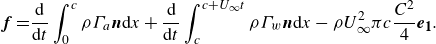 \begin{align} \boldsymbol{f}=&\frac {\rm d}{{\rm d}t}\int _0^c \rho \Gamma _a \boldsymbol{n} {\rm d}x + \frac {\rm d}{{\rm d}t}\int _c^{c + U_\infty t} \rho \Gamma _w \boldsymbol{n} {\rm d}x-\rho U^2_\infty \pi c\frac {C^2}{4}\boldsymbol{e_1} . \end{align}
Taking now into account that $\alpha (t)\ll 1$
and
$\alpha (t)\ll 1$
and $h(t)/c\ll 1$
, the linearisation of the normal vector
$h(t)/c\ll 1$
, the linearisation of the normal vector $\boldsymbol{n}$
in equation (2.28) yields
$\boldsymbol{n}$
in equation (2.28) yields
 \begin{equation} \boldsymbol{n}\cdot \boldsymbol{e_2}\simeq 1\quad \mathrm{and}\quad \boldsymbol{n}\cdot \boldsymbol{e_1}=-\frac {\partial \,z_{a,w}(x,t)}{\partial \,x} . \end{equation}
Introducing the results of (2.28) and (2.29) into the definitions of $\ell (t)$
and
$\ell (t)$
and $d(t)$
, namely,
$d(t)$
, namely,
 \begin{equation} \ell (t)=\boldsymbol{e_2}\cdot \boldsymbol{f} ,\quad d(t)=\boldsymbol{e_1}\cdot \boldsymbol{f} , \end{equation}
provides us with the following equations for the lift and drag forces:
 \begin{equation} \ell (t)=\frac {\rm d}{{\rm d}t}\int _0^{c + U_\infty t} \! \rho \Gamma _{a,w} {\rm d}x , \quad d(t)=-\frac {\rm d}{{\rm d}t} \int _0^{c + U_\infty t} \! \rho \Gamma _{a,w} \frac {\partial z_{a,w}}{\partial x}\,{\rm d}x-\rho U^2_\infty c\pi \! \left (\frac {C}{2}\right )^2 . \end{equation}
Using the Leibniz rule for differentiation, we obtain the following equation for $\ell (t)$
:
$\ell (t)$
:
 \begin{align} \ell (t)&=\rho U_\infty \Gamma _w(c + U_\infty t) + \int _0^c \rho \frac {\partial \Gamma _a}{\partial t}\,{\rm d}x + \int _c^{c + U_\infty t}\rho \frac {\partial \Gamma _w}{\partial t}\,{\rm d}x \notag\\&=\rho U_\infty \Gamma _w(c + U_\infty t) + \int _0^c \rho \frac {\partial \Gamma _a}{\partial t}\,{\rm d}x-U_\infty \int _c^{c + U_\infty t}\rho \frac {\partial \Gamma _w}{\partial x}\,{\rm d}x \notag\\&=\rho \frac {\rm d}{{\rm d}t}\int _0^c \Gamma _a (x,t)\,{\rm d}x + \rho U_\infty \Gamma _a(x=c,t) , \end{align}
where we have made use of (2.8) and of the fact that $\Gamma _w(x=c,t)=\Gamma _a(x=c,t)$
. Equation (2.32) reveals that the expression for the lift force calculated through a momentum balance coincides with the one obtained by direct integration of the pressure distribution around the airfoil, see (2.7) and (2.13).
$\Gamma _w(x=c,t)=\Gamma _a(x=c,t)$
. Equation (2.32) reveals that the expression for the lift force calculated through a momentum balance coincides with the one obtained by direct integration of the pressure distribution around the airfoil, see (2.7) and (2.13).
Next, we recover a similar equation for the drag force to that deduced by Fernandez-Feria (Reference Fernandez-Feria2016) once $d(t)$
in (2.31) is integrated by parts
$d(t)$
in (2.31) is integrated by parts
 \begin{align} d(t)&=-\rho \frac {\rm d}{{\rm d}t}\int _0^{c + U_\infty t} \frac {\partial }{\partial x} \left (\Gamma _{a,w} z_{a,w}\right )\,{\rm d}x + \rho \frac {\rm d}{{\rm d}t}\int _0^{c + U_\infty t} z_{a,w} \gamma _{a,w}(x,t)\,{\rm d}x \notag\\&\quad-\rho U^2_\infty c\pi \left (\frac {C}{2}\right )^2 \notag\\&=\rho \frac {\rm d}{{\rm d}t}\!\int _0^{c} \! z_{a}(x,t) \gamma _{a}(x,t)\,{\rm d}x + \rho \frac {\rm d}{{\rm d}t}\!\int _c^{c + U_\infty t}\! z_{w}(x,t) \gamma _w(x,t)\,{\rm d}x-\rho U^2_\infty c\pi \!\left (\frac {C}{2}\right )^2 , \end{align}
where we have taken into account that $\Gamma (x=0)=\Gamma (x=c + U_\infty t)=0$
and also that
$\Gamma (x=0)=\Gamma (x=c + U_\infty t)=0$
and also that $z_a$
and
$z_a$
and $z_w$
are bounded. Notice that the last term in (2.33), which was not included in Fernandez-Feria (Reference Fernandez-Feria2016), represents the contribution to the thrust force of the momentum flux which is being ejected horizontally by the starting vortex.
$z_w$
are bounded. Notice that the last term in (2.33), which was not included in Fernandez-Feria (Reference Fernandez-Feria2016), represents the contribution to the thrust force of the momentum flux which is being ejected horizontally by the starting vortex.
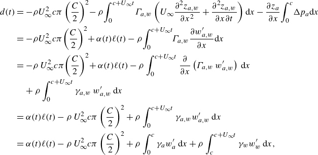
In this contribution, however, the thrust force, $-d(t)$
, will be calculated using the Leibniz rule for differentiation and, hence, we deduce from (2.31) that
$-d(t)$
, will be calculated using the Leibniz rule for differentiation and, hence, we deduce from (2.31) that
 \begin{align} d(t)&=-\rho U^2_\infty c\pi \left (\frac {C}{2}\right )^2-\rho \Gamma _w U_\infty \frac {\partial z_w}{\partial x}(x=c + U_\infty t) -\int _0^{c + U_\infty t} \rho \Gamma _{a,w} \frac {\partial ^2 z_{a,w}}{\partial x\partial t}{\rm d}x\notag \\&\quad + \int _0^{c + U_\infty t} \rho U_\infty \frac {\partial z_{a,w}}{\partial x}\frac {\partial \Gamma _{a,w}}{\partial x}\, {\rm d}x-\frac {\partial z_a}{\partial x}\int _0^{c}\Delta p_a {\rm d}x , \end{align}
where we have made use of the Bernoulli equation (2.7). Taking now into account that
 \begin{equation} \frac {\partial z_{a,w}}{\partial x}\frac {\partial \Gamma _{a,w}}{\partial x}=\frac {\partial }{\partial x}\left (\Gamma _{a,w} \frac {\partial z_{a,w}}{\partial x}\right )-\Gamma _{a,w}\frac {\partial ^2 z_{a,w}}{\partial x^2} , \end{equation}
and also that $\Gamma _a(x=0)=0$
, (2.34) reads
$\Gamma _a(x=0)=0$
, (2.34) reads
 \begin{align} d(t) & =-\rho U^2_\infty c\pi \left (\frac {C}{2}\right )^2\!-\rho \!\int _0^{c + U_\infty t} \!\Gamma _{a,w} \left (U_\infty \frac {\partial ^2 z_{a,w}}{\partial x^2} + \frac {\partial ^2 z_{a,w}}{\partial x\partial t}\right ){\rm d}x-\frac {\partial z_a}{\partial x}\!\int _0^c \!\Delta p_a {\rm d}x \notag \\&=-\rho U^2_\infty c\pi \!\left (\frac {C}{2}\right )^2\! + \alpha (t)\ell (t)-\rho \!\int _0^{c + U_\infty t}\!\!\Gamma _{a,w} \frac {\partial w'_{a,w}}{\partial x}{\rm d}x \notag \\& = -\rho \,U^2_\infty c\pi \!\left (\frac {C}{2}\right )^2\! + \alpha (t)\ell (t) -\rho \int _0^{c + U_\infty t} \frac {\partial }{\partial x}\left (\Gamma _{a,w}\,w'_{a,w}\right )\,{\rm d}x \notag \\& \quad + \rho \int _0^{c + U_\infty t} \gamma _{a,w}\,w'_{a,w}\,{\rm d}x \notag \\&=\alpha (t)\ell (t)-\rho \,U^2_\infty c\pi \left (\frac {C}{2}\right )^2 + \rho \int _0^{c + U_\infty t}\gamma _{a,w} w'_{a,w}\,{\rm d}x \notag \\&=\alpha (t)\ell (t)-\rho \,U^2_\infty c\pi \left (\frac {C}{2}\right )^2 + \rho \int _0^{c}\gamma _{a} w'_{a}\,{\rm d}x + \rho \int _c^{c + U_\infty t}\gamma _{w} w'_{w}\,{\rm d}x , \end{align}
where we have made use of (2.1) and of (2.4) and have taken into account that $\Gamma _a w'_a(x\rightarrow 0)\rightarrow 0$
and
$\Gamma _a w'_a(x\rightarrow 0)\rightarrow 0$
and $\Gamma _w w'_w(x\rightarrow c + U_\infty t)\rightarrow 0$
because
$\Gamma _w w'_w(x\rightarrow c + U_\infty t)\rightarrow 0$
because $\Gamma _a(x=0)=\Gamma _w(x=c + U_\infty t)=0$
and
$\Gamma _a(x=0)=\Gamma _w(x=c + U_\infty t)=0$
and $w'_{a,w}$
are bounded. In (2.36), the first term is the projection in the flight direction of the lift force whereas the second one is the contribution to the thrust force of the flux of horizontal momentum induced by the starting vortex. The third and fourth terms are the result of the Kutta equation, which expresses that the force in the direction perpendicular to the velocity
$w'_{a,w}$
are bounded. In (2.36), the first term is the projection in the flight direction of the lift force whereas the second one is the contribution to the thrust force of the flux of horizontal momentum induced by the starting vortex. The third and fourth terms are the result of the Kutta equation, which expresses that the force in the direction perpendicular to the velocity $V$
of a vortex with circulation
$V$
of a vortex with circulation $\Gamma$
is
$\Gamma$
is $\rho V \Gamma$
and, hence, the integral term in (2.36) is nothing but the contribution to the horizontal force of all vortices with circulation
$\rho V \Gamma$
and, hence, the integral term in (2.36) is nothing but the contribution to the horizontal force of all vortices with circulation ${\rm d}\Gamma (x,t)=\gamma _{a,w}(x,t){\rm d}x$
on which the vertical velocity is
${\rm d}\Gamma (x,t)=\gamma _{a,w}(x,t){\rm d}x$
on which the vertical velocity is $w'_{a,w}(x,t)$
.
$w'_{a,w}(x,t)$
.
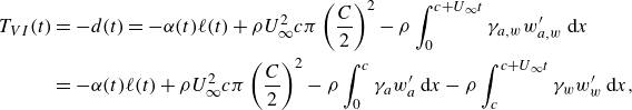
Consequently, the thrust force calculated using the vortex impulse theory reads
 \begin{align} T_{VI}(t)&=-d(t)=-\alpha (t)\ell (t) + \rho U^2_\infty c\pi \left (\frac {C}{2}\right )^2-\rho \int _0^{c + U_\infty t}\gamma _{a,w} w'_{a,w}\,{\rm d}x \notag\\&=-\alpha (t)\ell (t) + \rho U^2_\infty c\pi \left (\frac {C}{2}\right )^2-\rho \int _0^{c}\gamma _{a} w'_{a}\,{\rm d}x-\rho \int _c^{c + U_\infty t}\gamma _{w} w'_{w}\,{\rm d}x, \end{align}
where we have made use of (2.36) and the subscript $VI$
indicates vortex impulse. Notice that, by analogy with the vortex force resulting from the volume integral of
$VI$
indicates vortex impulse. Notice that, by analogy with the vortex force resulting from the volume integral of $\rho (\nabla \times \boldsymbol{v} )\times \boldsymbol{v}$
see e.g. Saffman (Reference Saffman1993), the third term at the right-hand side of (2.37) represents the vortex thrust force associated with the vortices in the airfoil whereas the fourth term represents the vortex thrust force associated with the vortices in the wake.
$\rho (\nabla \times \boldsymbol{v} )\times \boldsymbol{v}$
see e.g. Saffman (Reference Saffman1993), the third term at the right-hand side of (2.37) represents the vortex thrust force associated with the vortices in the airfoil whereas the fourth term represents the vortex thrust force associated with the vortices in the wake.
In order to compare the result in (2.37) with the analogous equation derived in Fernandez-Feria (Reference Fernandez-Feria2016), it is shown in Appendix B that the result in (2.37) can be expressed as
 \begin{align} &T_{VI}(t)=-\alpha (t)\ell (t) + \rho U^2_\infty c\pi \left (\frac {C}{2}\right )^2 + \frac {\rho \pi \dot {\alpha }c^2}{4}\left (-\dot {h}-U_\infty \alpha (t) + x_c\dot {\alpha }\right )\notag\\& + \rho \frac {c}{2}\int _1^{1 + 2U_\infty t/c}\left [-\dot {h}-U_\infty \alpha + x_c \dot {\alpha } + \frac {c}{2}\dot {\alpha }\left (\sqrt {\chi ^2-1}-\chi \right )-w'_w(\chi ,t)\right ]\gamma _w(\chi ,t)\,{\rm d}\chi ,\end{align}
with dots denoting time derivatives, ${\rm d}/{\rm d}t$
, and
${\rm d}/{\rm d}t$
, and
 \begin{equation} \chi =\frac {x-\dfrac{c}{2}}{\dfrac{c}{2}} ,\quad x_e=\frac {c}{2} + x_c , \end{equation}
with $x_e$
in (2.1) indicating the horizontal position of the pitching axis. The equation for the thrust force corresponding to the permanent response of airfoils oscillating periodically deduced in Fernandez-Feria (Reference Fernandez-Feria2016) and Sanchez-Laulhe et al. (Reference Sanchez-Laulhe, Fernandez-Feria and Ollero2023) is similar to (2.38) once it is noticed that
$x_e$
in (2.1) indicating the horizontal position of the pitching axis. The equation for the thrust force corresponding to the permanent response of airfoils oscillating periodically deduced in Fernandez-Feria (Reference Fernandez-Feria2016) and Sanchez-Laulhe et al. (Reference Sanchez-Laulhe, Fernandez-Feria and Ollero2023) is similar to (2.38) once it is noticed that $h_{FF}(t)=-h(t)$
– with the subscript
$h_{FF}(t)=-h(t)$
– with the subscript $FF$
indicating from now on Fernández-Feria – and once the upper limit of the integral is set to
$FF$
indicating from now on Fernández-Feria – and once the upper limit of the integral is set to $\infty$
, but contains crucial differences from our result. Indeed, two of the terms in (2.38) are missing in (29) and (31) of Fernandez-Feria (Reference Fernandez-Feria2016), namely, the term
$\infty$
, but contains crucial differences from our result. Indeed, two of the terms in (2.38) are missing in (29) and (31) of Fernandez-Feria (Reference Fernandez-Feria2016), namely, the term $\rho U^2_\infty c\pi (C/2 )^2$
, which represents the contribution to the thrust force of the starting vortex, and also the term
$\rho U^2_\infty c\pi (C/2 )^2$
, which represents the contribution to the thrust force of the starting vortex, and also the term
 \begin{equation} -\rho \int _c^{c + U_\infty t}\gamma _{w} w'_{w}\,{\rm d}x , \end{equation}
which represents the vortex thrust force associated with the vortices in the wake.
Let us also explain here that the reason why the term (2.40) is missing in Fernandez-Feria (Reference Fernandez-Feria2016, Reference Fernandez-Feria2017), Alaminos-Quesada & Fernandez-Feria (Reference Alaminos-Quesada and Fernandez-Feria2020) and Sanchez-Laulhe et al. (Reference Sanchez-Laulhe, Fernandez-Feria and Ollero2023) is a consequence of an assumption made in Fernandez-Feria (Reference Fernandez-Feria2016). Indeed, (25) in Fernandez-Feria (Reference Fernandez-Feria2016) expresses that $z_w(x,t)=z_w(x-U_\infty t)$
, with this assumption implying, by virtue of (2.4), that
$z_w(x,t)=z_w(x-U_\infty t)$
, with this assumption implying, by virtue of (2.4), that $w'_{w}=\partial z_w/\partial t + U_\infty \partial z_w/\partial x=0$
. However, there is no need to assume any functional dependence for
$w'_{w}=\partial z_w/\partial t + U_\infty \partial z_w/\partial x=0$
. However, there is no need to assume any functional dependence for $z_w(x,t)$
because the vertical velocity
$z_w(x,t)$
because the vertical velocity $w'_{a,w}(z=0,x,t)$
is the one induced by the vortex sheet extending along the airfoil and the wake, namely,
$w'_{a,w}(z=0,x,t)$
is the one induced by the vortex sheet extending along the airfoil and the wake, namely,
 \begin{equation} w'_{a,w}(z=0,x,t)=\frac {1}{2\pi }\int _0^{c + U_\infty t} \frac {\gamma _{a,w}(x_0,t)}{x_0-x}\,{\rm d}x_0 , \end{equation}
which is clearly different from zero for $x\gt c$
i.e.
$x\gt c$
i.e. $w'_w(z=0,x,t)\neq 0$
, as will be also illustrated in § 3.
$w'_w(z=0,x,t)\neq 0$
, as will be also illustrated in § 3.
It will be shown next that, if the vertical velocities of the wake vortices, $w'_w(x,t)$
, are calculated self-consistently, namely, making use of (2.41), the thrust force calculated using the vortex impulse theory is identical to the one calculated by direct integration of the pressure distribution around the airfoil i.e.
$w'_w(x,t)$
, are calculated self-consistently, namely, making use of (2.41), the thrust force calculated using the vortex impulse theory is identical to the one calculated by direct integration of the pressure distribution around the airfoil i.e. $T_G(t)=T_{VI}(t)$
, see (2.22) and (2.37), for any type of motion of the airfoil, which could be impulsive, oscillatory, etc.
$T_G(t)=T_{VI}(t)$
, see (2.22) and (2.37), for any type of motion of the airfoil, which could be impulsive, oscillatory, etc.
Indeed, introducing equation (2.41) into (2.37), the equation for the thrust force (2.37) reads
 \begin{equation} T_{VI}(t)=-\alpha (t)\ell (t) + \rho U^2_\infty c\pi \left (\!\frac {C}{2}\!\right )^2\!-\frac {\rho }{2\pi }\!\int _0^{c + U_\infty t}\!\gamma _{a,w}(x,t) {\rm d}x\!\int _0^{c + U_\infty t} \!\frac {\gamma _{a,w}(x_0,t)}{x_0-x} {\rm d}x_0. \end{equation}
The comparison between (2.22) and (2.42) reveals that these two equations would provide us with an identical result if
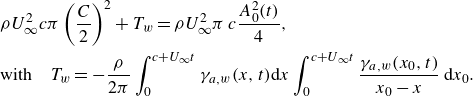 \begin{align} &\rho U^2_\infty c\pi \left (\frac {C}{2}\right )^2 + T_w=\rho U^2_\infty \pi \,c \frac {A^2_0(t)}{4} ,\notag\\&\mathrm{with}\quad T_w=-\frac {\rho }{2\pi }\int _0^{c + U_\infty t}\gamma _{a,w}(x,t) {\rm d}x\int _0^{c + U_\infty t} \frac {\gamma _{a,w}(x_0,t)}{x_0-x} \,{\rm d}x_0 . \end{align}
In order to prove this is so, we first introduce the following changes of variables:
 \begin{equation} \frac {x}{a(t)}=\frac {1-\cos \theta }{2} ,\!\!\quad \frac {x_0}{a(t)}=\frac {1-\cos \theta _0}{2}\Rightarrow {\rm d}x=a(t)\frac {\sin \theta }{2}\,{\rm d}\theta \!\!\quad \mathrm{and}\!\!\quad {\rm d}x_0=a(t)\frac {\sin \theta _0}{2}\,{\rm d}\theta _0 ,\end{equation}
with
 \begin{equation} a(t)=c + U_\infty t . \end{equation}
Now notice that: (i) $\Gamma (x=0)=\Gamma (x=a(t))=0$
, (ii) by virtue of (2.17) and taking into account that
$\Gamma (x=0)=\Gamma (x=a(t))=0$
, (ii) by virtue of (2.17) and taking into account that $\Gamma (x/c\ll 1,t)=2\phi '(x/c\ll 1,z=0^ + ,t)$
and also that, in polar coordinates, the point
$\Gamma (x/c\ll 1,t)=2\phi '(x/c\ll 1,z=0^ + ,t)$
and also that, in polar coordinates, the point $(z=0^ + ,x/c\gt 0)$
on the airfoil corresponds to
$(z=0^ + ,x/c\gt 0)$
on the airfoil corresponds to $(r/c=x/c,\beta =0)$
, the value of the circulation in close proximity to the leading edge is
$(r/c=x/c,\beta =0)$
, the value of the circulation in close proximity to the leading edge is $\Gamma (x/c\ll 1,t)=2 A_0(t) U_\infty \sqrt {x c}$
, (iii) if the airfoil is suddenly set into motion at
$\Gamma (x/c\ll 1,t)=2 A_0(t) U_\infty \sqrt {x c}$
, (iii) if the airfoil is suddenly set into motion at $t=0^ + $
,
$t=0^ + $
, $\Gamma (x\approx a(t))=2 C\,U_\infty \sqrt { (a(t) -x ) c}$
, see (2.27), then the circulation density along the airfoil and the wake can be expressed, in terms of the variable
$\Gamma (x\approx a(t))=2 C\,U_\infty \sqrt { (a(t) -x ) c}$
, see (2.27), then the circulation density along the airfoil and the wake can be expressed, in terms of the variable $\theta \in [0,\pi ]$
defined in (2.44), as
$\theta \in [0,\pi ]$
defined in (2.44), as
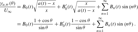 \begin{align} \frac {\gamma _{a,w}(\theta )}{U_\infty }&=B_0(t)\sqrt {\frac {a(t)-x}{x}} + B'_0(t)\sqrt {\frac {x}{a(t)-x}} + \sum _{n=1}^\infty B_n(t)\sin \left (n\theta \right )\notag\\& =B_0(t)\frac {1 + \cos \theta }{\sin \theta } + B'_0(t)\frac {1-\cos \theta }{\sin \theta } + \sum _{n=1}^\infty B_n(t)\sin \left (n\theta \right ) . \end{align}
Making use of (2.44)–(2.46), the perturbed vertical velocity given by (2.41) can be expressed as
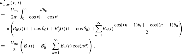 \begin{align}\begin{split}&w'_{a,w}(x,t)\\& = -\frac{U_\infty}{2\pi}\int_0^\pi\frac{d\theta_0}{\cos\theta_0-\cos\theta}\\& \quad \times \! \left( \! B_0(t) \!\left(1+\cos\theta_0\right)+B'_0(t)\!\left(1-\cos\theta_0\right)+ \!\sum_{n=1}^\infty \! B_n(t)\frac{\cos\!\left[(n-1)\theta_0\right]-\cos \!\left[(n+1)\theta_0\right]}{2} \! \right)\\&=-\frac{U_\infty}{2}\left(B_0(t)-B'_0-\sum_{n=1}^\infty B_n(t)\cos(n\theta)\right),\end{split}\end{align}
where we have made use of the well-known result (Glauert Reference Glauert1983)
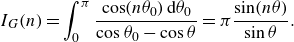 \begin{equation} I_G(n)=\int _0^\pi \frac {\cos (n\theta _0)\,{\rm d}\theta _0}{\cos \theta _0-\cos \theta }=\pi \frac {\sin (n\theta )}{\sin \theta } . \end{equation}
Finally, introducing the results of (2.44)–(2.47) into (2.43) yields
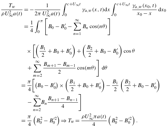 \begin{align} \frac {T_w}{\rho U^2_\infty a(t)} & = -\frac {1}{2\pi \,U^2_\infty a(t)}\int _0^{c + U_\infty t}\gamma _{a,w}(x,t) {\rm d}x\int _0^{c + U_\infty t} \frac {\gamma _{a,w}(x_0,t)}{x_0-x}\,{\rm d}x_0 \notag\\&=\frac {1}{4}\int _0^\pi \left [B_0-B'_0-\sum _{n=1}^\infty B_n\cos (n\theta )\right ]\notag \\ & \quad \times\left [\left (\frac {B_1}{2} + B_0 + B'_0\right ) + \left (\frac {B_2}{2} + B_0-B'_0\right )\cos \theta \right. \nonumber \\ & \left. \quad + \sum _{m=2}^\infty \frac {B_{m + 1}-B_{m-1}}{2}\cos (m\theta )\right ]\,{\rm d}\theta \notag \\&=\frac {\pi }{4}\!\left [\left (B_0-B'_0\right )\times \left (\frac {B_1}{2} + B_0 + B'_0\right )-\frac {B_1}{2}\left (\frac {B_2}{2} + B_0-B'_0\right ) \right. \nonumber \\ & \left. \quad - \sum _{n=2}^\infty \! B_n\frac {B_{n + 1}-B_{n-1}}{4}\right ]\notag \\&=\frac {\pi }{4}\left (B^2_0-B'^2_0\right )\Rightarrow T_w=\frac {\rho U^2_\infty \pi a(t)}{4}\left (B^2_0-B'^2_0\right ) . \end{align}
The comparison between (2.46) and (2.17) and (2.27) at both the leading edge and at the position where the starting vortex is located, namely, $x/c\ll 1$
and
$x/c\ll 1$
and $(a(t)-x)/c\ll 1$
, indicates that
$(a(t)-x)/c\ll 1$
, indicates that
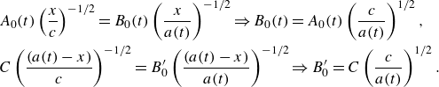 \begin{align} & A_0(t)\left (\frac{x}{c}\right )^{-1/2}=B_0(t)\left (\frac{x}{a(t)}\right )^{-1/2}\Rightarrow B_0(t)=A_0(t)\left (\frac{c}{a(t)}\right )^{1/2} , \notag\\ & C\left (\frac{(a(t)-x)}{c}\right )^{-1/2}=B'_0\left (\frac{(a(t)-x)}{a(t)}\right )^{-1/2}\Rightarrow B'_0=C\left (\frac{c}{a(t)}\right )^{1/2} . \end{align}
The substitution of the results in (2.50) into (2.49) yields
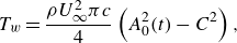 \begin{equation} T_w=\frac {\rho U^2_\infty \pi c}{4}\left (A^2_0(t)-C^2\right ) , \end{equation}
from which we conclude that (2.43) is satisfied, a fact meaning that the thrust force calculated using the vortex impulse theory through either of (2.37), (2.38), (2.42), is identical to the one calculated by direct integration of the pressures around the airfoil, see (2.22), i.e.
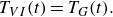 \begin{equation} T_{VI}(t)=T_G(t) . \end{equation}
The result in (2.52), which simply expresses that the force calculated by means of the integration of pressures around the airfoil is identical to the one obtained through a momentum balance, permits us to conclude that the correct equations for the thrust force within the linearised potential flow approach are (2.22) or either of (2.37), (2.38), (2.42). Hence, for the particular case in which the airfoil oscillates periodically, the correct equations for the thrust force within the linearised approach and in the limit $t U_\infty /c\rightarrow \infty$
are either the one deduced by Garrick (Reference Garrick1936), or either of (2.37), (2.38), (2.42) deduced using a momentum balance, once the upper limits of the integrals are set to
$t U_\infty /c\rightarrow \infty$
are either the one deduced by Garrick (Reference Garrick1936), or either of (2.37), (2.38), (2.42) deduced using a momentum balance, once the upper limits of the integrals are set to $\infty$
. This conclusion contradicts the assertions in Fernandez-Feria (Reference Fernandez-Feria2016, Reference Fernandez-Feria2017) and Alaminos-Quesada & Fernandez-Feria (Reference Alaminos-Quesada and Fernandez-Feria2020), where it is stated that the formulation in Fernandez-Feria (Reference Fernandez-Feria2016) corrects the theory due to Garrick.
$\infty$
. This conclusion contradicts the assertions in Fernandez-Feria (Reference Fernandez-Feria2016, Reference Fernandez-Feria2017) and Alaminos-Quesada & Fernandez-Feria (Reference Alaminos-Quesada and Fernandez-Feria2020), where it is stated that the formulation in Fernandez-Feria (Reference Fernandez-Feria2016) corrects the theory due to Garrick.
3. Numerical evidence showing the relevance of the starting vortex and of the vertical velocities of the vortices in the wake to predicting thrust
This section illustrates, through several numerical results, the main conclusion drawn from § 2, namely, that the thrust force calculated using the vortex impulse theory is identical to the force calculated by direct integration of the pressure distribution around the airfoil. The numerical examples to be shown below have also been selected with the purpose of illustrating that, when the force is evaluated using the vortex impulse theory within the linearised potential flow approach, it is essential to retain the two terms that were missing in (29)–(31) of Fernandez-Feria (Reference Fernandez-Feria2016), namely, the term which represents the contribution of the starting vortex to thrust and the term (2.40), which represents the vortex thrust force associated with the vortices in the wake, see (2.38). In this section, we will also consider the case in which the airfoil is suddenly set into motion and, moreover, we will discuss the limits of applicability of the linearised potential flow theory.
With all these purposes in mind, it proves convenient to define first the dimensionless thrust forces resulting from all contributions to thrust in (2.22) and (2.37), (2.38), (2.42) except the one expressing the projection in the flight direction of the normal force to the airfoil, namely,
 \begin{equation} \Delta t_G=\frac {T_G(t) + \alpha (t)\ell (t)}{\rho U^2_\infty c}=\pi \, \frac {A^2_0(t)}{4}, \end{equation}
and
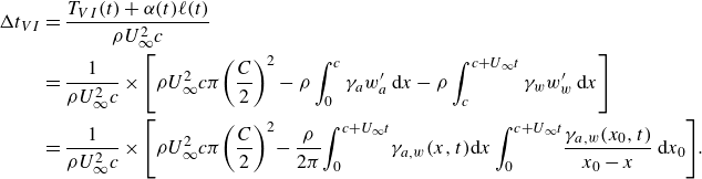 \begin{align} \Delta t_{VI} & =\frac {T_{VI}(t) + \alpha (t)\ell (t)}{\rho U_\infty ^2 c}\notag\\&=\frac {1}{\rho U^2_\infty c}\times \left [\rho U^2_\infty c\pi \! \left (\frac {C}{2}\right )^2-\rho \int _0^{c}\gamma _{a} w'_{a}\,{\rm d}x-\rho \int _c^{c + U_\infty t}\gamma _{w} w'_{w}\,{\rm d}x\right ]\notag\\&=\frac {1}{\rho U^2_\infty c}\times \left [\rho U^2_\infty c\pi \! \left (\frac {C}{2}\right )^2 \! - \frac {\rho }{2\pi } \! \int _0^{c + U_\infty t} \! \gamma _{a,w}(x,t) {\rm d}x\int _0^{c + U_\infty t} \! \frac {\gamma _{a,w}(x_0,t)}{x_0-x} \,{\rm d}x_0\right ]\! . \end{align}
The values of $\Delta t_G(\tau )$
and of
$\Delta t_G(\tau )$
and of $\Delta t_{VI}(\tau )$
defined in (3.1)–(3.2), where the dimensionless time,
$\Delta t_{VI}(\tau )$
defined in (3.1)–(3.2), where the dimensionless time, $\tau$
, is defined as
$\tau$
, is defined as
 \begin{equation} \tau =\frac {2\,U_\infty t}{c} , \end{equation}
have been calculated in the examples depicted below using the numerical code, based on the vortex-lattice method, detailed in the Supplementary Material.
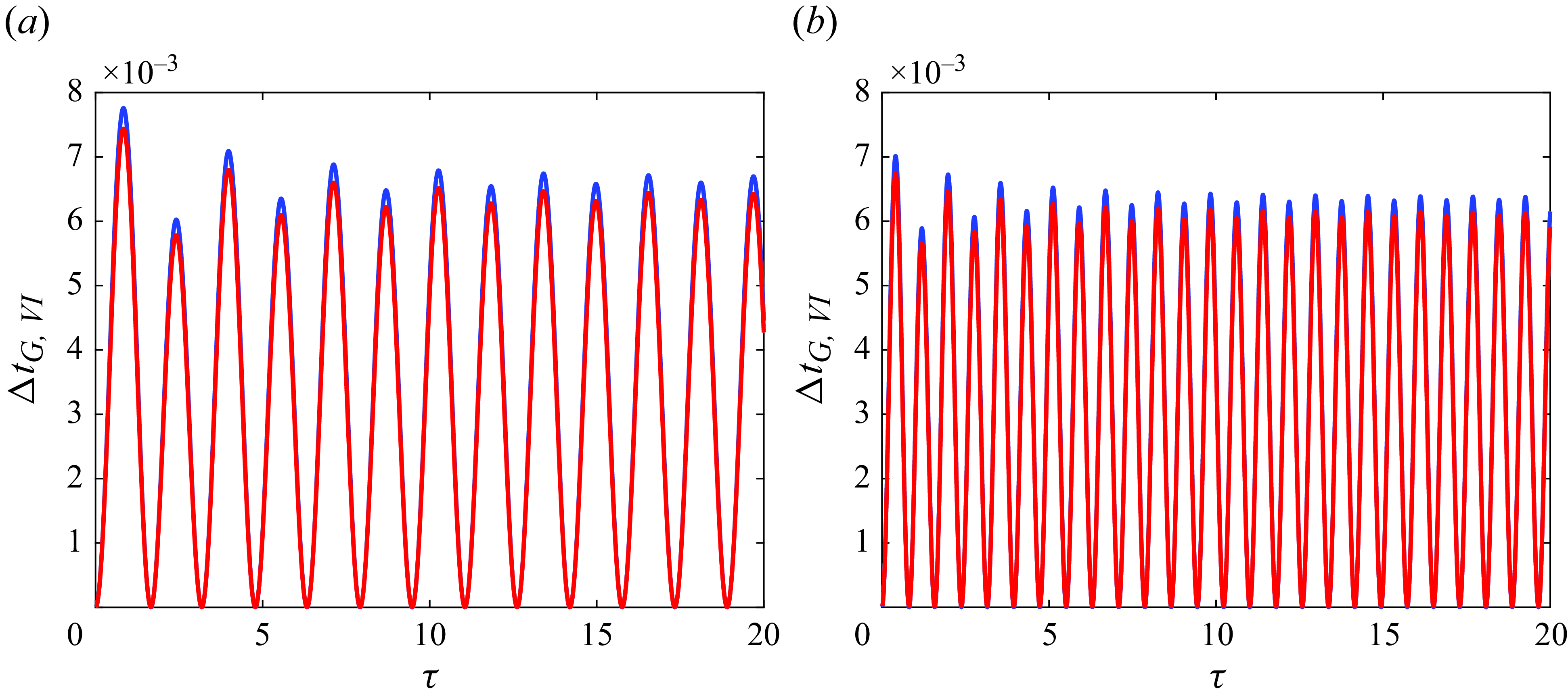
Figure 2. Dimensionless thrust forces $\Delta t_G(\tau )$
(blue line) and
$\Delta t_G(\tau )$
(blue line) and $\Delta t_{VI}(\tau )$
(red line) respectively defined in (3.1) and (3.2), corresponding to the plunging motion prescribed by (3.4), for two different values of the reduced frequency:
$\Delta t_{VI}(\tau )$
(red line) respectively defined in (3.1) and (3.2), corresponding to the plunging motion prescribed by (3.4), for two different values of the reduced frequency: $(a)$
$(a)$ $k=2$
and
$k=2$
and $(b)$
$(b)$ $k=4$
. Notice that both results coincide at every instant of time, as expected from the result in (2.52).
$k=4$
. Notice that both results coincide at every instant of time, as expected from the result in (2.52).
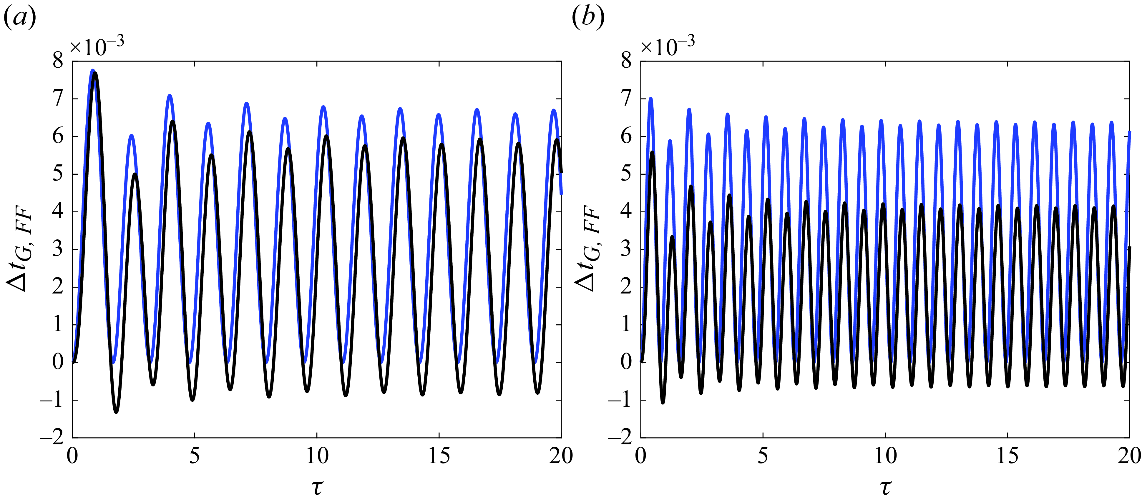
Figure 3. Dimensionless thrust forces $\Delta t_G(\tau )$
(blue line) and
$\Delta t_G(\tau )$
(blue line) and $\Delta t_{FF}(\tau )$
(black line) respectively defined in (3.1) and (3.6), corresponding to the plunging motion prescribed by (3.4), for two different values of the reduced frequency:
$\Delta t_{FF}(\tau )$
(black line) respectively defined in (3.1) and (3.6), corresponding to the plunging motion prescribed by (3.4), for two different values of the reduced frequency: $(a)$
$(a)$ $k=2$
and
$k=2$
and $(b)$
$(b)$ $k=4$
. Notice that the differences between the values of
$k=4$
. Notice that the differences between the values of $\Delta t_G(\tau )$
and of
$\Delta t_G(\tau )$
and of $\Delta t_{FF}(\tau )$
increase with the value of the reduced frequency
$\Delta t_{FF}(\tau )$
increase with the value of the reduced frequency $k$
. Moreover, the results in the figure show that the mean thrust corresponding to
$k$
. Moreover, the results in the figure show that the mean thrust corresponding to $\Delta t_{FF}$
is smaller than the mean thrust corresponding to
$\Delta t_{FF}$
is smaller than the mean thrust corresponding to $\Delta t_{G}$
, and also that the differences between the values of the mean thrust become more pronounced for the larger value of the reduced frequency. The results depicted in figures 2 and 3 will be discussed in more detail in § 4, where an equation for the mean thrust coefficient is deduced.
$\Delta t_{G}$
, and also that the differences between the values of the mean thrust become more pronounced for the larger value of the reduced frequency. The results depicted in figures 2 and 3 will be discussed in more detail in § 4, where an equation for the mean thrust coefficient is deduced.
We first consider the case in which an oscillating airfoil performs a purely plunging motion with a frequency $\omega$
and with a vertical velocity given by
$\omega$
and with a vertical velocity given by
 \begin{equation} \frac {w'_a(0\leqslant x\leqslant c,t)}{U_\infty }=-V\sin \left (\omega \,t\right )=-V\sin \left (k\tau \right )\quad \mathrm{with}\quad V=\frac {5\pi }{180}, \end{equation}
with $k$
in (3.4) indicating the so-called reduced frequency, defined as
$k$
in (3.4) indicating the so-called reduced frequency, defined as
 \begin{equation} k=\frac {\omega c}{2\,U_\infty } . \end{equation}
Since $w'_a(0\leqslant x\leqslant c,t=0^ + )=0$
,
$w'_a(0\leqslant x\leqslant c,t=0^ + )=0$
, $C=0$
in (3.2) and, hence, the contribution of the starting vortex to thrust is also zero for the case considered in (3.4), see also Appendix A.
$C=0$
in (3.2) and, hence, the contribution of the starting vortex to thrust is also zero for the case considered in (3.4), see also Appendix A.
The results in figures 2 and 3, corresponding to the plunging motion defined in (3.4), illustrate the relevance of the term (2.40), representing the vortex thrust force of the vortices in the wake. Indeed, notice first that, as expected from (2.52), the results depicted in figure 2 confirm that the value of the thrust forces, calculated by either the integration of the pressure distribution around the airfoil or using the vortex impulse theory, are very close to each other, with the tiny differences between the two results attributable to the effect of the numerical discretisation in the evaluation of the integrals in the definition of $\Delta t_{VI}(\tau )$
, see (3.2). Next, figure 3 compares the values of
$\Delta t_{VI}(\tau )$
, see (3.2). Next, figure 3 compares the values of $\Delta t_G(\tau )$
depicted in figure 2 with the values of the dimensionless thrust force defined as
$\Delta t_G(\tau )$
depicted in figure 2 with the values of the dimensionless thrust force defined as
 \begin{align} &\Delta t_{FF}(\tau )=\Delta t_{VI}(\tau )-\frac {1}{\rho U^2_\infty c}\times \left [\rho U^2_\infty c\pi \left (\frac {C}{2}\right )^2-\rho \int _c^{c + U_\infty t}\gamma _{w} w'_{w}\,{\rm d}x\right ] , \end{align}
with $\Delta t_{VI}(\tau )$
given in (3.2) and which represents the dimensionless thrust force calculated using the vortex impulse theory under the assumptions made in Fernandez-Feria (Reference Fernandez-Feria2016), namely, once the contributions of the starting vortex – which is zero for the particular case of the plunging motion considered in (3.4) – and of the contribution of the vortex thrust force of the vortices in the wake, see (2.40), are set to zero. The results depicted in figure 3 reveal that the values of
$\Delta t_{VI}(\tau )$
given in (3.2) and which represents the dimensionless thrust force calculated using the vortex impulse theory under the assumptions made in Fernandez-Feria (Reference Fernandez-Feria2016), namely, once the contributions of the starting vortex – which is zero for the particular case of the plunging motion considered in (3.4) – and of the contribution of the vortex thrust force of the vortices in the wake, see (2.40), are set to zero. The results depicted in figure 3 reveal that the values of $\Delta t_{G}(\tau )$
and of
$\Delta t_{G}(\tau )$
and of $\Delta t_{FF}(\tau )$
are not identical to each other and, in fact, the differences between
$\Delta t_{FF}(\tau )$
are not identical to each other and, in fact, the differences between $\Delta t_{G}(\tau )$
and
$\Delta t_{G}(\tau )$
and $\Delta t_{FF}(\tau )$
become more visible as the value of the reduced frequency
$\Delta t_{FF}(\tau )$
become more visible as the value of the reduced frequency $k$
is increased; notice that the differences between the values of the mean thrust depicted in figures 2 and 3 will be discussed in more depth in § 4. Using the results depicted in figure 2 and also those in (3.2) and (3.6), we can infer that the values of
$k$
is increased; notice that the differences between the values of the mean thrust depicted in figures 2 and 3 will be discussed in more depth in § 4. Using the results depicted in figure 2 and also those in (3.2) and (3.6), we can infer that the values of $\Delta t_G(\tau )$
and of
$\Delta t_G(\tau )$
and of $\Delta t_{FF}(\tau )$
would be identical if
$\Delta t_{FF}(\tau )$
would be identical if $w'_w(x\gt c,t)=0$
. However, this is not the case, as can be appreciated in figure 4, which shows that, in fact, the amplitudes of the vertical velocities in the wake increase with the value of
$w'_w(x\gt c,t)=0$
. However, this is not the case, as can be appreciated in figure 4, which shows that, in fact, the amplitudes of the vertical velocities in the wake increase with the value of $k$
, despite the value of
$k$
, despite the value of $V$
in (3.4) remaining unchanged. Notice also that figure 3 illustrates one of the main results deduced by Fernández-Feria: the mean thrust predicted in Fernandez-Feria (Reference Fernandez-Feria2016) is similar to the mean thrust predicted by Garrick’s theory for low-to-moderate values of the reduced frequency, but it is smaller than the mean thrust predicted by Garrick (Reference Garrick1936) for
$V$
in (3.4) remaining unchanged. Notice also that figure 3 illustrates one of the main results deduced by Fernández-Feria: the mean thrust predicted in Fernandez-Feria (Reference Fernandez-Feria2016) is similar to the mean thrust predicted by Garrick’s theory for low-to-moderate values of the reduced frequency, but it is smaller than the mean thrust predicted by Garrick (Reference Garrick1936) for $k\gtrsim O(1)$
. In view of the definitions in (3.1), (3.2) and (3.6) and of the conclusions in § 2, the reason for the differences depicted in figure 3 is that the results in Fernandez-Feria (Reference Fernandez-Feria2016) were obtained neglecting the vertical velocities of the wake vortices i.e. assuming that
$k\gtrsim O(1)$
. In view of the definitions in (3.1), (3.2) and (3.6) and of the conclusions in § 2, the reason for the differences depicted in figure 3 is that the results in Fernandez-Feria (Reference Fernandez-Feria2016) were obtained neglecting the vertical velocities of the wake vortices i.e. assuming that $w'_w(x,t)=0$
, which implies that the term (2.40) is also zero. However, the values of
$w'_w(x,t)=0$
, which implies that the term (2.40) is also zero. However, the values of $w'_w(x,t)$
calculated within the linearised potential flow theory by means of (2.41) are different from zero, as shown in figure 4 and, hence, the contribution to thrust of the vortex force in (2.40), cannot be neglected.
$w'_w(x,t)$
calculated within the linearised potential flow theory by means of (2.41) are different from zero, as shown in figure 4 and, hence, the contribution to thrust of the vortex force in (2.40), cannot be neglected.
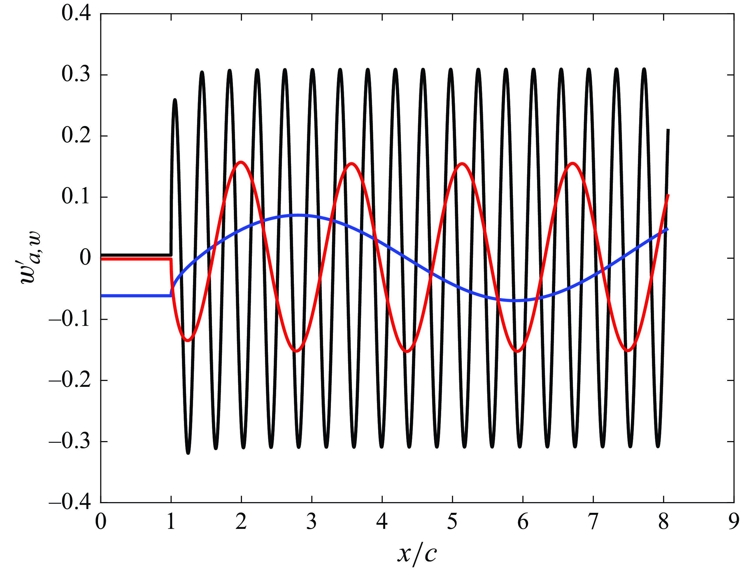
Figure 4. Vertical velocities induced by the vortex sheet extending along the airfoil and the wake calculated using (2.41). The results depicted in the figure correspond to the plunging motion defined in (3.4) for three different values of the reduced frequency: $k=8$
(black curve),
$k=8$
(black curve), $k=2$
(red curve) and
$k=2$
(red curve) and $k=0.5$
(blue curve). Notice that the amplitudes of the vertical velocities in the wake for the cases
$k=0.5$
(blue curve). Notice that the amplitudes of the vertical velocities in the wake for the cases $k=2$
and
$k=2$
and $k=8$
are clearly larger than the amplitude of the vertical airfoil velocity,
$k=8$
are clearly larger than the amplitude of the vertical airfoil velocity, $V=5\pi /180$
.
$V=5\pi /180$
.
Next, we consider the case in which an oscillating airfoil performs a purely plunging motion with a frequency $\omega$
and with a vertical velocity given by
$\omega$
and with a vertical velocity given by
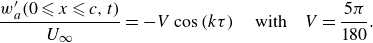 \begin{equation} \frac {w'_a(0\leqslant x\leqslant c,t)}{U_\infty }=-V\cos \left (k\tau \right )\quad \mathrm{with}\quad V=\frac {5\pi }{180} . \end{equation}
It is deduced in Appendix A that
 \begin{equation} C=\frac {w'_a(x=3c/4,t=0^ + )}{U_\infty }=-\left (\alpha _0 + \frac {\dot {h}_0}{U_\infty } + \frac {\dot {\alpha }_0}{U_\infty }\left (\frac {3c}{4}-x_e\right )\right ) , \end{equation}
with quantities with the subscript $0$
indicating their corresponding values at
$0$
indicating their corresponding values at $t=0^ + $
and, hence, the contribution of the starting vortex to the thrust force cannot be neglected if
$t=0^ + $
and, hence, the contribution of the starting vortex to the thrust force cannot be neglected if $w'_a(x=3c/4,t=0^ + )\neq 0$
. The results depicted in figure 5(a) confirm this is the case: indeed, the blue and black curves representing the values of
$w'_a(x=3c/4,t=0^ + )\neq 0$
. The results depicted in figure 5(a) confirm this is the case: indeed, the blue and black curves representing the values of $\Delta t_G(\tau )$
(blue) and of
$\Delta t_G(\tau )$
(blue) and of $\Delta t_{VI}(\tau )$
(black) defined in (3.1) and (3.2), are very close to each other. However, the red curve, which represents the numerical values of
$\Delta t_{VI}(\tau )$
(black) defined in (3.1) and (3.2), are very close to each other. However, the red curve, which represents the numerical values of
 \begin{equation} \Delta t_{VIB}=\Delta t_{VI}(\tau )-\frac {\pi C^2}{4} , \end{equation}
namely, of the thrust force calculated using the vortex impulse theory once the contribution of the starting vortex is set to zero, is well below the black and blue curves. Due to the fact that the value of the thrust force calculated using the vortex impulse theory must be identical to the value obtained by direct integration of the pressure distribution around the airfoil, the result depicted in figure 5(a) illustrates that the contribution of the starting vortex cannot be neglected for those cases in which $w'_a(x=3c/4,t=0^ + )\neq 0$
. Moreover, the results in figure 5(b) illustrate that, as expected, the thrust forces of the plunging motions corresponding to (3.4) and (3.7) converge to the same values with just a phase shift.
$w'_a(x=3c/4,t=0^ + )\neq 0$
. Moreover, the results in figure 5(b) illustrate that, as expected, the thrust forces of the plunging motions corresponding to (3.4) and (3.7) converge to the same values with just a phase shift.
Figure 5. $(a)$
Dimensionless thrust forces
$(a)$
Dimensionless thrust forces $\Delta t_G(\tau )$
(blue line) and
$\Delta t_G(\tau )$
(blue line) and $\Delta t_{VI}(\tau )$
(black line) defined, respectively, in (3.1) and (3.2), corresponding to the plunging motion of the airfoil prescribed by (3.7) for a value of the reduced frequency
$\Delta t_{VI}(\tau )$
(black line) defined, respectively, in (3.1) and (3.2), corresponding to the plunging motion of the airfoil prescribed by (3.7) for a value of the reduced frequency $k=2$
. Notice that both results coincide at every instant of time, as expected from the result expressed by (2.52). The red curve corresponds to the results of (3.9), which does not retain the effect of the starting vortex.
$k=2$
. Notice that both results coincide at every instant of time, as expected from the result expressed by (2.52). The red curve corresponds to the results of (3.9), which does not retain the effect of the starting vortex. $(b)$
After a short transient, the forces corresponding to the plunging motions defined in (3.4) – in blue – and (3.7) – in black – for a value of the reduced frequency
$(b)$
After a short transient, the forces corresponding to the plunging motions defined in (3.4) – in blue – and (3.7) – in black – for a value of the reduced frequency $k=2$
converge to the same result with just a phase shift.
$k=2$
converge to the same result with just a phase shift.
Finally, we analyse the case of an airfoil that is suddenly set into motion, for which
 \begin{equation} \frac {w'_a(0\leqslant x\leqslant c,t)}{U_\infty }=-\left (\alpha _0 + \frac {\dot {h}_0}{U_\infty } + \frac {\dot {\alpha }_0}{U_\infty }\left (x-x_e\right )\right )\,H(t) ,\end{equation}
with $H(t)$
indicating the Heaviside function. The lift force corresponding to (3.10) was calculated by Wagner (Reference Wagner1925) as, see also the Supplementary Material,
$H(t)$
indicating the Heaviside function. The lift force corresponding to (3.10) was calculated by Wagner (Reference Wagner1925) as, see also the Supplementary Material,
 \begin{equation} \ell _{Wagner}(\tau )=\rho U^2_\infty c\pi \left (-\frac {w'_a \!\left(x=\dfrac{3c}{4},t=0^+ \right)}{U_\infty }\right )\phi (\tau ), \end{equation}
with $\phi (\tau )$
the so-called Wagner function, which is approximated here using the well-known equation given by Jones (Reference Jones1938)
$\phi (\tau )$
the so-called Wagner function, which is approximated here using the well-known equation given by Jones (Reference Jones1938)
 \begin{equation} \phi (\tau )=1-0.165\,e^{-0.0455\,\tau }-0.335\,e^{-0.3\tau } , \end{equation}
whereas the corresponding expression for the thrust force is deduced in the Supplementary Material and reads
 \begin{align} T_{G,Wagner}(\tau )&=\rho U^2_\infty c\pi \frac {w'_a\!\left(x=\dfrac{3c}{4},t=0^+ \right)}{U_\infty }\phi (\tau )\alpha _0 \notag \\&\quad+\rho U^2_\infty c\pi \left (\frac {w'_a\!\left(x=\dfrac{3c}{4},t=0^+ \right)}{U_\infty }\phi (\tau )+\frac {c}{4U_\infty }\dot {\alpha }_0\right )^2 . \end{align}
Notice that a special case of (3.13) is given on page 705 of Donovan & Lawrence (Reference Donovan and Lawrence1957). Hence, for the case of the so-called Wagner problem, characterised by the linearised impenetrability boundary condition given by (3.10), we find that
 \begin{align} \Delta t_{G,Wagner}(\tau )&=\frac {T_{G,Wagner}(t)+\alpha _0\ell _{Wagner}(t)}{\rho U^2_\infty c}\notag\\&=\pi \left [\frac {w'_a\!\left(x= \dfrac{3c}{4},t=0^+ \right)}{U_\infty }\phi (\tau )+\frac {c\dot {\alpha }_0}{4U_\infty }\right ]^2 . \end{align}
Consistently with the results obtained in § 2 notice that, since the Wagner function verifies $\phi (\tau =0)=1/2$
, see (3.12) and the Supplementary Material for further details, the value of the thrust force given by (3.13) at
$\phi (\tau =0)=1/2$
, see (3.12) and the Supplementary Material for further details, the value of the thrust force given by (3.13) at $\tau =0$
,
$\tau =0$
, $T_{G,Wagner}(\tau =0)$
, coincides with the value of
$T_{G,Wagner}(\tau =0)$
, coincides with the value of $T_{VI}(\tau =0)$
calculated using (2.38).
$T_{VI}(\tau =0)$
calculated using (2.38).
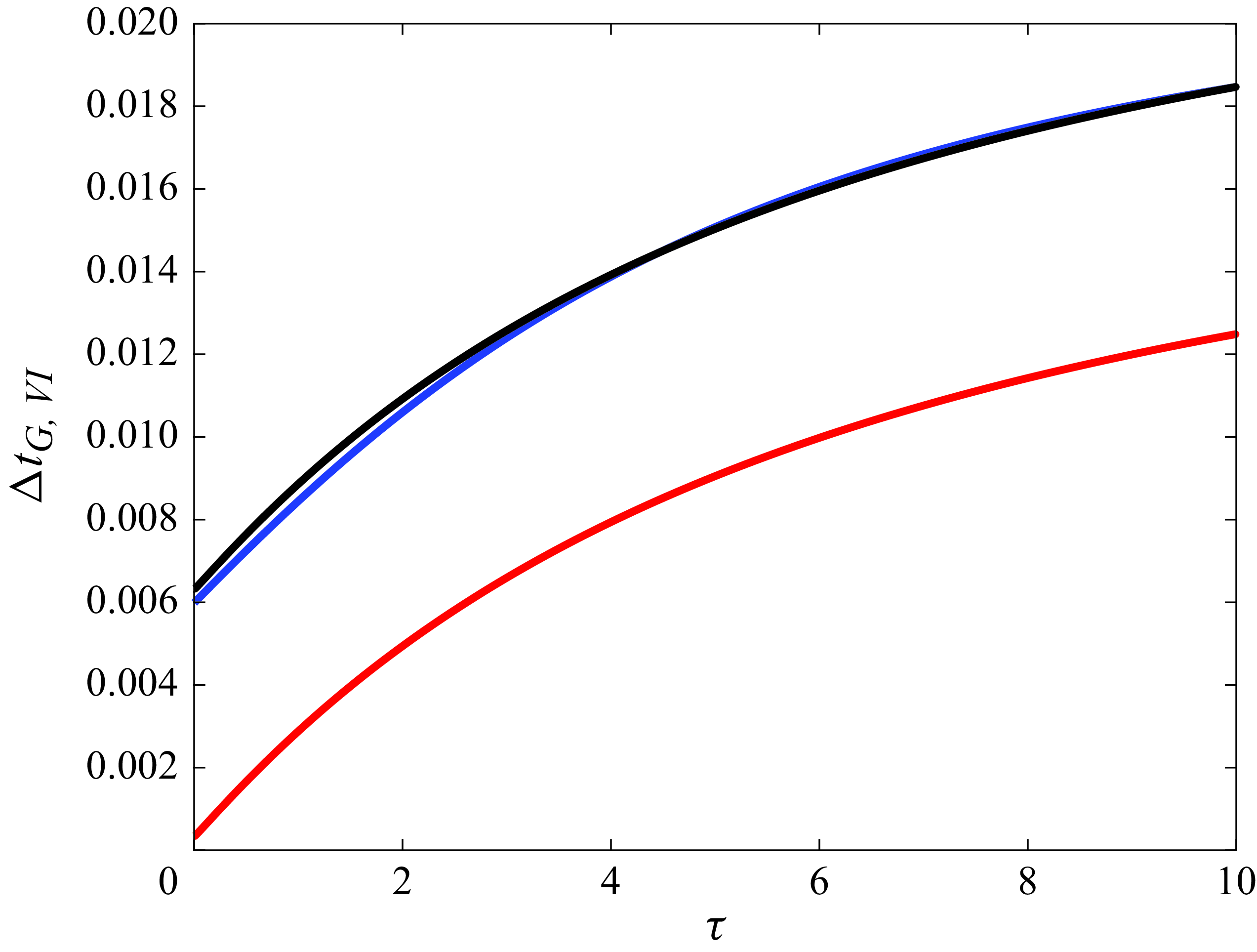
Figure 6. $(a)$
Dimensionless thrust forces corresponding to the impulsive motion of the airfoil prescribed by (3.15). Here,
$(a)$
Dimensionless thrust forces corresponding to the impulsive motion of the airfoil prescribed by (3.15). Here, $\Delta t_{VI}(\tau )$
(black line) and
$\Delta t_{VI}(\tau )$
(black line) and $\Delta t_{G,Wagner}(\tau )$
(blue line) have been calculated using (3.2) and (3.14), respectively. The red curve corresponds to the results of (3.9), which do not retain the effect of the starting vortex.
$\Delta t_{G,Wagner}(\tau )$
(blue line) have been calculated using (3.2) and (3.14), respectively. The red curve corresponds to the results of (3.9), which do not retain the effect of the starting vortex.
The numerical results in figure 6, corresponding to the impulsive motion of the airfoil given by
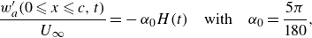 \begin{equation} \frac {w'_a(0\leqslant x\leqslant c,t)}{U_\infty }=-\,\alpha _0 H(t)\quad \mathrm{with}\quad \alpha _0=\frac {5\pi }{180} , \end{equation}
provides further support to (3.14) and also illustrates the relevance of the starting vortex in either of (2.37), (2.38), (2.42) to predict thrust when the airfoil is impulsively set into motion.
However, the ability of the prediction in (3.14) to reproduce experimental measurements is limited to those circumstances in which the starting hypotheses of the linearised potential flow theory are not violated. Indeed, notice that the dynamics of the starting vortex generated when the airfoil is suddenly set into motion is described by the self-similar solution found by Kaden (Reference Kaden1931), see also Pullin (Reference Pullin1978). The width of this self-similar region grows in time as $\propto (U_\infty \alpha ^{eq}_0c^{1/2} t )^{2/3}$
, with
$\propto (U_\infty \alpha ^{eq}_0c^{1/2} t )^{2/3}$
, with $\alpha ^{eq}_0$
indicating the equivalent angle of attack defined in (A4) of Appendix A. Hence, it is to be expected that, in a real experiment, the wake region surrounding the starting vortex experiences large deformations, causing a clear deviation from the linearised approximation, which assumes that the wake is located at
$\alpha ^{eq}_0$
indicating the equivalent angle of attack defined in (A4) of Appendix A. Hence, it is to be expected that, in a real experiment, the wake region surrounding the starting vortex experiences large deformations, causing a clear deviation from the linearised approximation, which assumes that the wake is located at $z=0$
. The deviations from the linearised approximation will take place for instants of time
$z=0$
. The deviations from the linearised approximation will take place for instants of time $t\gtrsim t^*$
, with
$t\gtrsim t^*$
, with $t^*$
estimated from
$t^*$
estimated from $ (U_\infty \alpha ^{eq}_0c^{1/2} t^* )^{2/3}\sim c$
and, hence,
$ (U_\infty \alpha ^{eq}_0c^{1/2} t^* )^{2/3}\sim c$
and, hence, $t^*\sim c/(U_\infty \alpha ^{eq}_0)\gg c/U_\infty$
if
$t^*\sim c/(U_\infty \alpha ^{eq}_0)\gg c/U_\infty$
if $\alpha ^{eq}_0\ll 1$
. The nonlinear rolling up of the starting vortex described above will certainly modify the thrust force predicted here for large times
$\alpha ^{eq}_0\ll 1$
. The nonlinear rolling up of the starting vortex described above will certainly modify the thrust force predicted here for large times $t\gtrsim t^*$
; clearly, the validity of our results pertaining to the thrust produced by the starting vortex, which have been deduced within linearised potential flow theory, should be checked against detailed numerical calculations at finite but high Reynolds numbers. However, this additional task exceeds the limits of the present contribution.
$t\gtrsim t^*$
; clearly, the validity of our results pertaining to the thrust produced by the starting vortex, which have been deduced within linearised potential flow theory, should be checked against detailed numerical calculations at finite but high Reynolds numbers. However, this additional task exceeds the limits of the present contribution.
Similarly, for the cases of airfoils oscillating periodically which are not suddenly set into motion and, hence, the effect of the starting vortex is negligible, the capability of the linearised potential flow results to predict the mean thrust forces is also limited to those cases in which the effect of nonlinearities can be neglected. However, there are a number of experimental conditions that trigger the development of nonlinearities, limiting the applicability of Garrick’s results. First, notice that the linearised approach will only be valid to predict experiments and numerical simulations if $H_0/c\ll 1$
, with
$H_0/c\ll 1$
, with $H_0$
denoting the characteristic amplitude of the oscillations, but this necessary condition is not sufficient. Indeed, it has been shown by Ramesh et al. (Reference Ramesh, Gopalarathnam, Granlund, Ol and Edwards2014), see also Eldredge (Reference Eldredge2019) that, in order to prevent flow separation and, hence, the associated ejection of vortices from the leading edge, it is necessary that the value of the adverse pressure gradient at
$H_0$
denoting the characteristic amplitude of the oscillations, but this necessary condition is not sufficient. Indeed, it has been shown by Ramesh et al. (Reference Ramesh, Gopalarathnam, Granlund, Ol and Edwards2014), see also Eldredge (Reference Eldredge2019) that, in order to prevent flow separation and, hence, the associated ejection of vortices from the leading edge, it is necessary that the value of the adverse pressure gradient at $x=0$
, which can be quantified through the value of
$x=0$
, which can be quantified through the value of $A_0$
in the expansion (2.19), is such that
$A_0$
in the expansion (2.19), is such that $A_0(t)\lesssim \alpha ^*$
, with
$A_0(t)\lesssim \alpha ^*$
, with $\alpha ^*\sim O(0.1)$
indicating a value which can be viewed as a critical angle of attack for flow separation. The value of
$\alpha ^*\sim O(0.1)$
indicating a value which can be viewed as a critical angle of attack for flow separation. The value of $\alpha ^*$
depends on the type of airfoil and needs to be calculated either experimentally or by means of full numerical simulations. For the case of an oscillating airfoil, the characteristic value of
$\alpha ^*$
depends on the type of airfoil and needs to be calculated either experimentally or by means of full numerical simulations. For the case of an oscillating airfoil, the characteristic value of $A_0$
can be estimated as the effective angle of attack resulting from the ratio between the characteristic vertical and horizontal velocities, namely,
$A_0$
can be estimated as the effective angle of attack resulting from the ratio between the characteristic vertical and horizontal velocities, namely, $A_0\sim \omega \,H_0/U_\infty$
. Hence, in order to prevent flow separation at the leading edge, it is necessary that
$A_0\sim \omega \,H_0/U_\infty$
. Hence, in order to prevent flow separation at the leading edge, it is necessary that $k\,H_0/c\lesssim \alpha ^*$
, with
$k\,H_0/c\lesssim \alpha ^*$
, with $k$
the reduced frequency defined in (3.5). In addition, even in the case that
$k$
the reduced frequency defined in (3.5). In addition, even in the case that $H_0/c\ll 1$
, the self-induced velocities of the vortices ejected from the trailing edge can cause large distortions in the wake for sufficiently large values of the reduced frequency: in fact, the vertical velocities in the wake are appreciably larger than the vertical velocities of the airfoil for large values of the reduced frequency, see figure 4. Indeed, the circulation around the airfoil can be estimated as
$H_0/c\ll 1$
, the self-induced velocities of the vortices ejected from the trailing edge can cause large distortions in the wake for sufficiently large values of the reduced frequency: in fact, the vertical velocities in the wake are appreciably larger than the vertical velocities of the airfoil for large values of the reduced frequency, see figure 4. Indeed, the circulation around the airfoil can be estimated as $\Gamma _e\sim U_\infty c A_0\sim c H_0\omega$
, with
$\Gamma _e\sim U_\infty c A_0\sim c H_0\omega$
, with $A_0$
estimated above and, moreover, the vertical velocity induced by the vortices ejected during a period of oscillation on the new vortices leaving the trailing edge of the airfoil can be estimated, making use of (2.12), as
$A_0$
estimated above and, moreover, the vertical velocity induced by the vortices ejected during a period of oscillation on the new vortices leaving the trailing edge of the airfoil can be estimated, making use of (2.12), as $w'_0\sim 1/U_\infty {\rm d}\Gamma _e/{\rm d}t\sim c H_0 \omega ^2/U_\infty$
. Hence, in order to prevent large deformations of the wake near the trailing edge of the airfoil, it is necessary that
$w'_0\sim 1/U_\infty {\rm d}\Gamma _e/{\rm d}t\sim c H_0 \omega ^2/U_\infty$
. Hence, in order to prevent large deformations of the wake near the trailing edge of the airfoil, it is necessary that $w'_0/U_\infty \lesssim O(1)$
, namely, that
$w'_0/U_\infty \lesssim O(1)$
, namely, that $(\omega \,H_0/U_\infty )^2 (H_0/c)^{-1}\lesssim O(1)$
or, equivalently, that
$(\omega \,H_0/U_\infty )^2 (H_0/c)^{-1}\lesssim O(1)$
or, equivalently, that $k^2 (H_0/c)\lesssim O(1)$
.
$k^2 (H_0/c)\lesssim O(1)$
.
The emergence of nonlinearities for values of the reduced frequency such that $k^2 (H_0/c)\gtrsim O(1)$
is evidenced, for instance, when the wake is non-planar, as is clearly depicted in the experiments by Godoy-Diana et al. (Reference Godoy-Diana, Aider and Wesfreid2008) or in the full numerical simulations by Young & Lai (Reference Young and Lai2004) and Martín-Alcántara et al. (Reference Martín-Alcántara, Fernandez-Feria and Sanmiguel-Rojas2015). In these references, the vortices in the wake are arranged in such a way that the vertical component of their self-induced velocities is negligible, as is evidenced by the fact that the wake vortices in these references are convected horizontally. We hypothesise that it is under these circumstances that the predictions in Fernandez-Feria (Reference Fernandez-Feria2016, Reference Fernandez-Feria2017) agree better with experiments than Garrick’s theory. The reason for this is that, when the vortices are convected horizontally,
$k^2 (H_0/c)\gtrsim O(1)$
is evidenced, for instance, when the wake is non-planar, as is clearly depicted in the experiments by Godoy-Diana et al. (Reference Godoy-Diana, Aider and Wesfreid2008) or in the full numerical simulations by Young & Lai (Reference Young and Lai2004) and Martín-Alcántara et al. (Reference Martín-Alcántara, Fernandez-Feria and Sanmiguel-Rojas2015). In these references, the vortices in the wake are arranged in such a way that the vertical component of their self-induced velocities is negligible, as is evidenced by the fact that the wake vortices in these references are convected horizontally. We hypothesise that it is under these circumstances that the predictions in Fernandez-Feria (Reference Fernandez-Feria2016, Reference Fernandez-Feria2017) agree better with experiments than Garrick’s theory. The reason for this is that, when the vortices are convected horizontally, $w'_w\approx 0$
and, hence, the projection of
$w'_w\approx 0$
and, hence, the projection of $\rho (\nabla \times \boldsymbol{v} )\times \boldsymbol{v}$
on the flight direction is negligible, making the contribution of the vortex force term (2.40) also negligible in the real nonlinear flow. Clearly, these nonlinear effects cannot be accounted for by the theory developed by Garrick (Reference Garrick1936) or by the self-consistent vortex impulse results presented here, which predict that the vertical velocities of the wake vortices is different from zero, as can be appreciated in figure 4.
$\rho (\nabla \times \boldsymbol{v} )\times \boldsymbol{v}$
on the flight direction is negligible, making the contribution of the vortex force term (2.40) also negligible in the real nonlinear flow. Clearly, these nonlinear effects cannot be accounted for by the theory developed by Garrick (Reference Garrick1936) or by the self-consistent vortex impulse results presented here, which predict that the vertical velocities of the wake vortices is different from zero, as can be appreciated in figure 4.
Then, the capability of the results in Fernandez-Feria (Reference Fernandez-Feria2016, Reference Fernandez-Feria2017) to predict both experiments and numerical results for values of the reduced frequency of order unity or larger, for which the wake experiences large deformations, seems to be justified by the fact that the results in Fernandez-Feria (Reference Fernandez-Feria2016, Reference Fernandez-Feria2017) correspond to a linearised model which takes into account realistic nonlinear effects.
The discussion above permits us to conclude that, if the conditions of a particular experiment in which the airfoil oscillates periodically are such that the effects of nonlinearities are negligible and, hence, the starting hypotheses of the linearised potential flow approach are valid, the thrust force should be calculated using the self-consistent results expressed by (2.22) or by either of (2.37), (2.38), (2.42). This explains why the experimental measurements of the mean thrust in Mackowski & Williamson (Reference Mackowski and Williamson2015) can be reasonably well predicted by Garrick’s theory, which should be then used for small values of the reduced frequency once viscous effects are taken into consideration, see e.g. Figure 3(a) in Fernandez-Feria (Reference Fernandez-Feria2017). However, when nonlinearities are triggered and the vortices in the wake are arranged in such a way that their vertical self-induced velocities are negligible, namely, $w'_w\approx 0$
, the linearised model in Fernandez-Feria (Reference Fernandez-Feria2016, Reference Fernandez-Feria2017) and Alaminos-Quesada & Fernandez-Feria (Reference Alaminos-Quesada and Fernandez-Feria2020) should be used instead, once the modifications to the equation for the mean thrust coefficient pointed out in § 4 are taken into account, because the contribution to thrust of the vortex force term (2.40) is not calculated self-consistently within the linearised potential flow approach in these contributions but, instead, it is assumed to be zero. The value of the thrust force deduced by Fernandez-Feria (Reference Fernandez-Feria2016, Reference Fernandez-Feria2017), once the modifications in the mean thrust coefficient deduced in § 4 are taken into account, happens to be a better approximation to the real value than the one obtained by means of the self-consistent linearised theory because, when the vortices in the wake are arranged in such a way that they are convected horizontally, the projection on the flight direction of
$w'_w\approx 0$
, the linearised model in Fernandez-Feria (Reference Fernandez-Feria2016, Reference Fernandez-Feria2017) and Alaminos-Quesada & Fernandez-Feria (Reference Alaminos-Quesada and Fernandez-Feria2020) should be used instead, once the modifications to the equation for the mean thrust coefficient pointed out in § 4 are taken into account, because the contribution to thrust of the vortex force term (2.40) is not calculated self-consistently within the linearised potential flow approach in these contributions but, instead, it is assumed to be zero. The value of the thrust force deduced by Fernandez-Feria (Reference Fernandez-Feria2016, Reference Fernandez-Feria2017), once the modifications in the mean thrust coefficient deduced in § 4 are taken into account, happens to be a better approximation to the real value than the one obtained by means of the self-consistent linearised theory because, when the vortices in the wake are arranged in such a way that they are convected horizontally, the projection on the flight direction of $\rho (\nabla \times \boldsymbol{v} )\times \boldsymbol{v}$
in the wake is zero, which implies that the contribution to the total vortex force of the vortices in the wake is also zero in the real, nonlinear case.
$\rho (\nabla \times \boldsymbol{v} )\times \boldsymbol{v}$
in the wake is zero, which implies that the contribution to the total vortex force of the vortices in the wake is also zero in the real, nonlinear case.
4. Mean thrust coefficient for the case of airfoils oscillating periodically when the wake vortices are convected downstream at the free-stream velocity
For those common cases in which the airfoil starts accelerating smoothly, namely, $C=0$
in (2.37), and the wake vortices are convected in a direction parallel to the free-stream velocity as a consequence of the development of nonlinearities, which implies that
$C=0$
in (2.37), and the wake vortices are convected in a direction parallel to the free-stream velocity as a consequence of the development of nonlinearities, which implies that $w'_w=0$
, the thrust force is (see (2.37))
$w'_w=0$
, the thrust force is (see (2.37))
 \begin{align} T_{VI}(t)=-\alpha (t)\ell (t)-\rho \int _0^{c}\gamma _{a} w'_{a}\,{\rm d}x , \end{align}
which is identical to the one used in Fernandez-Feria (Reference Fernandez-Feria2016), as has been discussed in the derivation of (2.38).
In this section, our purpose will be to deduce an equation for the thrust force averaged in time when the airfoil oscillates periodically with a frequency $\omega$
, the wake vortices are convected with the incident velocity and the contribution of the starting vortex to thrust is set to zero. For that purpose, we first make use of the fact that, since
$\omega$
, the wake vortices are convected with the incident velocity and the contribution of the starting vortex to thrust is set to zero. For that purpose, we first make use of the fact that, since $w'_a(x,t)=-\dot {h}-U_\infty \alpha -\dot {\alpha } (x-x_e )$
and
$w'_a(x,t)=-\dot {h}-U_\infty \alpha -\dot {\alpha } (x-x_e )$
and
 \begin{equation} \int _0^c\gamma _a(x,t)\,{\rm d}x=\Gamma _a(x=c,t)=\Gamma _e(t) ,\quad \frac {\partial }{\partial \,x}\left (\Gamma _aw'_a\right )=\gamma _aw'_a-\dot {\alpha }\Gamma _a ,\end{equation}
then
 \begin{align} -\rho \int _0^{c}\gamma _{a} w'_{a}\,{\rm d}x&=-\rho \left [-\left (\dot {h} + U_\infty \alpha + \dot {\alpha }\left (c-x_e\right )\right )\Gamma _e(t) + \dot {\alpha }\int _0^c \Gamma _a\,{\rm d}x\right ]\notag\\&=\rho \left (\dot {h} + \dot {\alpha }(t)\left (c-x_e\right )\right )\Gamma _e(t)-\rho \frac {\rm d}{{\rm d}t}\left (\alpha \int _0^c\Gamma _a\,{\rm d}x\right )\notag\\&\quad + \alpha (t)\left (\rho U_\infty \,\Gamma _e(t) + \rho \frac {\rm d}{{\rm d}t}\int _0^c \Gamma _a\,{\rm d}x\right ) , \end{align}
where we have made use of the fact that $\Gamma _a(x=0,t)=0$
and of the identity
$\Gamma _a(x=0,t)=0$
and of the identity
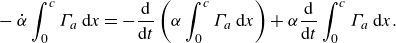 \begin{equation} -\dot {\alpha }\int _0^c\Gamma _a\,{\rm d}x=-\frac {\rm d}{{\rm d}t}\left (\alpha \int _0^c\Gamma _a\,{\rm d}x\right ) + \alpha \frac {\rm d}{{\rm d}t}\int _0^c \Gamma _a\,{\rm d}x . \end{equation}
The substitution of (4.3) into (4.1) yields that
 \begin{align} &T_{VI}(t)=\rho \left (\dot {h} + \dot {\alpha }(t)\left (c-x_e\right )\right )\Gamma _e(t)-\rho \frac {\rm d}{{\rm d}t}\left (\alpha \int _0^c\Gamma _a\,{\rm d}x\right ) , \end{align}
where we have made use of the expression for the lift force $\ell (t)$
in (2.32). Consequently, the mean thrust force can be calculated as
$\ell (t)$
in (2.32). Consequently, the mean thrust force can be calculated as
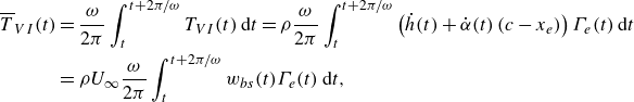 \begin{align} \overline {T}_{VI}(t)&=\frac {\omega }{2\pi }\int _t^{t + 2\pi /\omega } T_{VI}(t)\,{\rm d}t=\rho \frac {\omega }{2\pi }\int _t^{t + 2\pi /\omega } \left (\dot {h}(t) + \dot {\alpha }(t)\left (c-x_e\right )\right )\Gamma _e(t)\,{\rm d}t\notag\\&=\rho U_\infty \frac {\omega }{2\pi }\int _t^{t + 2\pi /\omega } w_{bs}(t)\Gamma _e(t)\,{\rm d}t , \end{align}
where we have taken into account that, since the thrust is a periodic function of time,
 \begin{equation} \int _t^{t + 2\pi /\omega }\,\frac {\rm d}{{\rm d}t}\left (\alpha \int _0^c\Gamma _a\,{\rm d}x\right )\,{\rm d}t=0 ,\end{equation}
and
 \begin{equation} w_{bs}(t)= \frac{\left (\dot {h}(t) + \dot {\alpha }(t)\left (c-x_e\right )\right )}{U_\infty} \, \end{equation}
denotes minus the dimensionless velocity of the trailing edge of the airfoil and, consequently,
 \begin{equation} \frac{-w'}{U_\infty}\left(\frac{x}{c}=\frac{3}{4},t\right)= \frac{-w'_{3/4}(t)}{U_\infty} =w_{bs}(t)+ \frac{\left(\alpha \,U_\infty - \dfrac{\dot {\alpha } c}{4}\right )}{U_\infty} . \end{equation}
The result in (4.6) expresses that, for those cases in which the airfoil oscillates periodically, the contribution of the starting vortex to thrust is negligible and the vortices in the wake are arranged in such a way that they are convected with a velocity parallel to the free-stream velocity, the mean thrust is proportional to the mean of the product of minus the vertical velocity of the trailing edge and the circulation around the airfoil. From now on, since we are considering the case of airfoils oscillating periodically, any generic time-dependent function $s(t)$
will be expressed as the real part of
$s(t)$
will be expressed as the real part of
 \begin{equation} s(t)=s^*\,e^{i k\tau } , \end{equation}
where the constant $s^*$
is a complex number,
$s^*$
is a complex number, $k=\omega c/(2\,U_\infty )$
is the reduced frequency and
$k=\omega c/(2\,U_\infty )$
is the reduced frequency and $\tau = 2t U_\infty /c$
refers to the dimensionless time.
$\tau = 2t U_\infty /c$
refers to the dimensionless time.
Using the results in e.g. Ashley & Landahl (Reference Ashley and Landahl1985) or in section V of the Supplementary Material, the analytical expression for the time-periodic circulation around the airfoil, namely, $\Gamma _e(t)=\pi U_\infty c (A_0(\tau ) + A_1(\tau )/2 )/2$
, is given by the real part of
$\Gamma _e(t)=\pi U_\infty c (A_0(\tau ) + A_1(\tau )/2 )/2$
, is given by the real part of
 \begin{equation} \Gamma _e(t)=\frac {\pi U_\infty c}{2}\,\frac {G^*}{i\,k}\,e^{i k\tau } , \end{equation}
where we have made use of the notation in (4.10). In (4.11), see Ashley & Landahl (Reference Ashley and Landahl1985) or section V of the Supplementary Material,
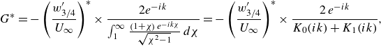 \begin{equation}G^*=-\left(\frac{w'_{3/4}}{U_\infty}\right)^*\times\frac{2e^{-i k}}{\int_1^\infty \frac{\left(1+\chi\right)\,e^{-ik\chi}}{\sqrt{\chi^2-1}}\,d\chi}=-\left(\frac{w'_{3/4}}{U_\infty}\right)^*\times\frac{2\,e^{-i k}}{K_0(ik)+K_1(ik)} ,\end{equation}
where $K_n$
in (4.12) indicates the modified Bessel function of the second kind of order
$K_n$
in (4.12) indicates the modified Bessel function of the second kind of order $n$
. Now, using the results in (4.9), (4.10) and the fact that
$n$
. Now, using the results in (4.9), (4.10) and the fact that ${\rm d}/{\rm d}t= (2U_\infty /c ) {\rm d}/{\rm d}\tau$
 \begin{align} &\left (\frac{-w'_{3/4}}{U_\infty}\right )^*=w_{bs}^* + a_0e^{i\phi }\left (1- \frac{ik}{2}\right ) ,\quad w_{bs}^*=2ik\left [\left (\frac{h_0}{c}\right ) + a_0 e^{i\phi }\left (1 - \frac{x_e}{c}\right )\right ] , \end{align}
with $h(t)=h_0\mathcal{R}(e^{ik\tau })$
,
$h(t)=h_0\mathcal{R}(e^{ik\tau })$
, $\alpha (t)=a_0\mathcal{R}(e^{i\phi } e^{ik\tau })$
,
$\alpha (t)=a_0\mathcal{R}(e^{i\phi } e^{ik\tau })$
, $h_0$
,
$h_0$
, $a_0$
real numbers indicating the amplitudes of the heaving and the pitching motions and
$a_0$
real numbers indicating the amplitudes of the heaving and the pitching motions and $\phi$
the phase shift. The substitution of (4.12) and (4.13) into (4.11) yields
$\phi$
the phase shift. The substitution of (4.12) and (4.13) into (4.11) yields
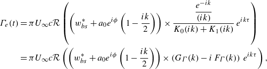 \begin{align} \Gamma _e(t)&=\pi U_\infty c\mathcal{R}\left (\left (w_{bs}^* + a_0e^{i\phi }\left (1- \frac{ik}{2}\right )\right )\times \frac {\dfrac{e^{-i k}}{(ik)}}{K_0(ik) + K_ 1(ik)}\,e^{i k\tau }\right )\notag\\&=\pi U_\infty c\mathcal{R}\left (\left (w_{bs}^* + a_0e^{i\phi }\left (1- \frac{ik}{2}\right )\right )\times \left (G_\Gamma (k)-i\,F_\Gamma (k)\right )\,e^{i k\tau }\right ), \end{align}
where
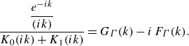 \begin{equation} \frac {\dfrac{e^{-i k}}{(ik)}}{K_0(ik) + K_1(ik)}=G_\Gamma (k)-i\,F_\Gamma (k) . \end{equation}
The functions $F_\Gamma (k)$
and
$F_\Gamma (k)$
and $G_\Gamma (k)$
in (4.15) are related with the analogous functions
$G_\Gamma (k)$
in (4.15) are related with the analogous functions $F_1(k)$
and
$F_1(k)$
and $G_1(k)$
defined in Fernandez-Feria (Reference Fernandez-Feria2016) in the following way:
$G_1(k)$
defined in Fernandez-Feria (Reference Fernandez-Feria2016) in the following way:
 \begin{equation} F_1(k)=-\left (\frac{\pi}{2}\right )\,F_\Gamma (k) ,\quad G_1(k)=-\left (\frac{\pi}{2}\right )\,G_\Gamma (k) . \end{equation}
For our subsequent purposes, it proves convenient to define here the function
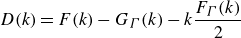 \begin{equation} D(k)=F(k)-G_\Gamma(k)-k\frac{F_\Gamma(k)}{2} \end{equation}
where $F(k)$
is the real part of the well-known Theodorsen function
$F(k)$
is the real part of the well-known Theodorsen function $C(k)$
, defined as
$C(k)$
, defined as
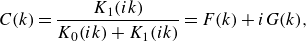 \begin{equation} C(k)=\frac {K_1(ik)}{K_0(ik) + K_1(ik)}=F(k) + iG(k), \end{equation}
see, e.g. Ashley & Landahl (Reference Ashley and Landahl1985) or section V of the Supplementary Material. The different functions $G_\Gamma (k)$
,
$G_\Gamma (k)$
, $F_\Gamma (k)$
and
$F_\Gamma (k)$
and $D(k)$
defined in (4.15) and (4.17) are plotted in figure 7.
$D(k)$
defined in (4.15) and (4.17) are plotted in figure 7.


Now, making use of the fact that: (i) all time-dependent functions are of the form given in (4.10) and (ii) the real part of a complex number $s^*$
is
$s^*$
is $(s^* + s^{*c})/2$
, with the superscript
$(s^* + s^{*c})/2$
, with the superscript $c$
affecting the complex variable
$c$
affecting the complex variable $s^*$
indicating the complex conjugate of
$s^*$
indicating the complex conjugate of $s^*$
, the substitution of (4.8), (4.9) and (4.14) into (4.6) yields
$s^*$
, the substitution of (4.8), (4.9) and (4.14) into (4.6) yields
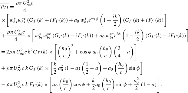 \begin{align} &\overline {T_{VI}}=\frac {\rho \pi U^2_\infty c}{4}\notag\\&\times \left [w_{bs}^* w_{bs}^{*c}\left (G_\Gamma (k)+iF_\Gamma (k)\right )+a_0\,w_{bs}^*e^{-i\phi }\left (1+ \frac{ik}{2}\right )\left (G_\Gamma (k)+iF_\Gamma (k)\right )\right ]\notag\\&+\frac {\rho \pi U^2_\infty c}{4}\times \left [w_{bs}^* w_{bs}^{*c}\left (G_\Gamma (k)-iF_\Gamma (k)\right )+a_0\,w_{bs}^{*c}e^{i\phi }\left (1-\frac{ik}{2}\right )\left (G_\Gamma (k)-iF_\Gamma (k)\right ) \right ]\notag\\&=2\rho \pi U^2_\infty c\,k^2G_\Gamma (k)\times \left [\left (\frac{h_0}{c}\right )^2+\cos \phi \,a_0\left (\frac{h_0}{c}\right )\left (\frac{3}{4}-a\right )\right ]\notag\\&+\rho \pi U^2_\infty c\,k\,G_\Gamma (k)\times \left [\frac{k}{2} \,a^2_0\left (1-a\right )\left (\frac{1}{2}-a\right )+a_0\left (\frac{h_0}{c}\right )\sin \phi \right ]\notag\\&-\rho \pi U^2_\infty c\,k\,F_\Gamma (k)\times \left [a_0\left (\frac{h_0}{c}\right )\cos \phi + \frac{k}{2} a_0\left (\frac{h_0}{c}\right )\sin \phi + \frac{a^2_0}{2}\left (1-a\right )\right ],\end{align}
and, hence, the expression of the mean thrust coefficient when the contributions to thrust of both the starting vortex and of the vortices in the wake are set to zero, is
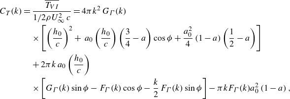 \begin{align} C_{T}(k)&=\frac {\overline {T_{VI}}}{1/2\rho U^2_\infty \,c}=4\pi k^2\,G_\Gamma (k)\notag\\& \quad \times\left [\left (\frac{h_0}{c}\right )^2 + \,a_0\left (\frac{h_0}{c}\right )\left (\frac{3}{4}-a\right )\cos \phi + \frac{a^2_0}{4}\left (1-a\right )\left (\frac{1}{2}-a\right )\right ] \nonumber \\ & \quad + 2\pi k \,a_0\left (\frac{h_0}{c}\right )\notag\\& \quad \times \left [G_\Gamma (k)\sin \phi - F_\Gamma (k)\cos \phi - \frac{k}{2}\,F_\Gamma (k)\sin \phi \right ] -\pi k F_\Gamma (k) a^2_0\left (1-a\right ) , \end{align}
where we have made use of the equation $x_e=(1 + a)c/2$
relating the position of the pitching axis
$x_e=(1 + a)c/2$
relating the position of the pitching axis $x_e$
with
$x_e$
with $a$
. The equation for the mean thrust coefficient given by (4.20), which does not take into account neither the vortex force term (2.40) nor the contribution of the starting vortex, differs from the mean thrust coefficient deduced by Garrick (Reference Garrick1936); see also (B4) in Fernandez-Feria (Reference Fernandez-Feria2016), reproduced here for clarity purposes
$a$
. The equation for the mean thrust coefficient given by (4.20), which does not take into account neither the vortex force term (2.40) nor the contribution of the starting vortex, differs from the mean thrust coefficient deduced by Garrick (Reference Garrick1936); see also (B4) in Fernandez-Feria (Reference Fernandez-Feria2016), reproduced here for clarity purposes
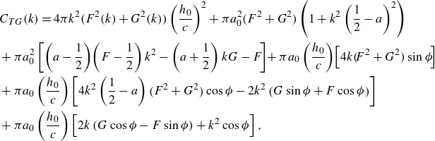 \begin{align} &C_{TG}(k)=4\pi k^2\big(F^2(k) + G^2(k)\big )\left(\frac{h_0}{c} \right)^2 + \pi a^2_0\big (F^2 + G^2\big )\left (1 + k^2\left (\frac{1}{2}-a\right )^2\right )\notag\\& + \pi a^2_0\left [\left (a-\frac{1}{2}\right )\!\left (F-\frac{1}{2}\right )k^2-\left (a + \frac{1}{2}\right )k G-F\!\right ]\! + \pi a_0\left (\frac{h_0}{c}\right )\!\left [4k \big (\!F^2 + G^2\big )\sin \phi \!\right ]\notag\\& + \pi a_0 \left(\frac{h_0}{c} \right)\left [4 k^2 \left (\frac{1}{2}-a\right )\big (F^2 + G^2\big )\cos \phi -2k^2\left (G\sin \phi + F\cos \phi \right )\right ]\notag\\& + \pi a_0 \left(\frac{h_0}{c} \right)\left [2k\left (G\cos \phi -F\sin \phi \right ) + k^2\cos \phi \right ] , \end{align}
where the functions $F(k)$
and
$F(k)$
and $G(k)$
are defined in (4.18). But (4.20) also differs from the analogous expression for the mean thrust coefficient given in (37) of Fernandez-Feria (Reference Fernandez-Feria2016), which was also deduced starting from (4.1) and was later on used by Fernandez-Feria (Reference Fernandez-Feria2017) in (A4)–(A6). Indeed, taking into account the result in (4.16) and once it is noticed that the dimensionless amplitude of the heaving motion in Fernandez-Feria (Reference Fernandez-Feria2016, Reference Fernandez-Feria2017),
$G(k)$
are defined in (4.18). But (4.20) also differs from the analogous expression for the mean thrust coefficient given in (37) of Fernandez-Feria (Reference Fernandez-Feria2016), which was also deduced starting from (4.1) and was later on used by Fernandez-Feria (Reference Fernandez-Feria2017) in (A4)–(A6). Indeed, taking into account the result in (4.16) and once it is noticed that the dimensionless amplitude of the heaving motion in Fernandez-Feria (Reference Fernandez-Feria2016, Reference Fernandez-Feria2017), $h_{FF}$
, is related to
$h_{FF}$
, is related to $\frac{h_0}{c}$
in (4.20) as
$\frac{h_0}{c}$
in (4.20) as $h_{FF}=-2(\frac{h_0}{c})$
, the mean thrust coefficient deduced by Fernandez-Feria (Reference Fernandez-Feria2016, Reference Fernandez-Feria2017) can be written as
$h_{FF}=-2(\frac{h_0}{c})$
, the mean thrust coefficient deduced by Fernandez-Feria (Reference Fernandez-Feria2016, Reference Fernandez-Feria2017) can be written as
 \begin{equation} C_{T,FF}(k)=C_{T}(k)-2\pi D(k)\times \left (a^2_0 + 2\,k\,a_0 \left(\frac{h_0}{c} \right)\sin \phi \right ) , \end{equation}
with $D(k)$
the function defined in (4.17) and plotted in figure 7 and where
$D(k)$
the function defined in (4.17) and plotted in figure 7 and where $C_T(k)$
is given in (4.20). Notice that the equation for the mean thrust deduced in Fernandez-Feria (Reference Fernandez-Feria2016), which has been written using our variables in (4.22), depends on the real part of Theodorsen’s function
$C_T(k)$
is given in (4.20). Notice that the equation for the mean thrust deduced in Fernandez-Feria (Reference Fernandez-Feria2016), which has been written using our variables in (4.22), depends on the real part of Theodorsen’s function $F(k)$
through the term
$F(k)$
through the term $D(k)$
– see (4.17) and (4.18), whereas the mean thrust coefficient deduced here in (4.20) only depends on the functions
$D(k)$
– see (4.17) and (4.18), whereas the mean thrust coefficient deduced here in (4.20) only depends on the functions $F_\Gamma (k)$
and
$F_\Gamma (k)$
and $G_\Gamma (k)$
defined in (4.15), which are related to the circulation around the airfoil, see (4.14). Notice also that, for the case of airfoils in purely heaving motion (
$G_\Gamma (k)$
defined in (4.15), which are related to the circulation around the airfoil, see (4.14). Notice also that, for the case of airfoils in purely heaving motion ( $a_0=0$
), (4.20) and (4.22) predict the same value for the mean thrust coefficient, a fact implying that our (4.20) is also in good agreement with experiments and numerical simulations for large values of the reduced frequency, as can be inferred from the results depicted in figure 5(a) of Fernandez-Feria (Reference Fernandez-Feria2016); however, (4.20) and (4.22) differ whenever
$a_0=0$
), (4.20) and (4.22) predict the same value for the mean thrust coefficient, a fact implying that our (4.20) is also in good agreement with experiments and numerical simulations for large values of the reduced frequency, as can be inferred from the results depicted in figure 5(a) of Fernandez-Feria (Reference Fernandez-Feria2016); however, (4.20) and (4.22) differ whenever $a_0\neq 0$
.
$a_0\neq 0$
.
Figure 8 compares the value of the mean thrust coefficient deduced by Garrick (Reference Garrick1936), which has been reproduced here using our notation in (4.21), with the one given in (4.20). The predictions of (4.20) and (4.21), corresponding to the cases of purely heaving and combined heaving and pitching motions, have been validated in figure 8 by means of the numerical results obtained using the method detailed in the Supplementary Material; notice that the numerical results are fairly close to those calculated through (4.20) and (4.21). In addition, as expected, the results in figure 8 reveal that the mean thrust coefficient calculated using (4.20), which corresponds to the case in which the contribution to thrust of the starting vortex is zero and the vortices in the wake are convected parallel to the free-stream velocity and, hence, the vortex force term in (2.40) is zero, is smaller than the mean thrust coefficient predicted by Garrick’s analysis, where the contribution of the vortices in the wake to the thrust force is different from zero. The results depicted in figure 8 and the accompanying discussion complete the analysis of the results shown in figures 2 and 3.
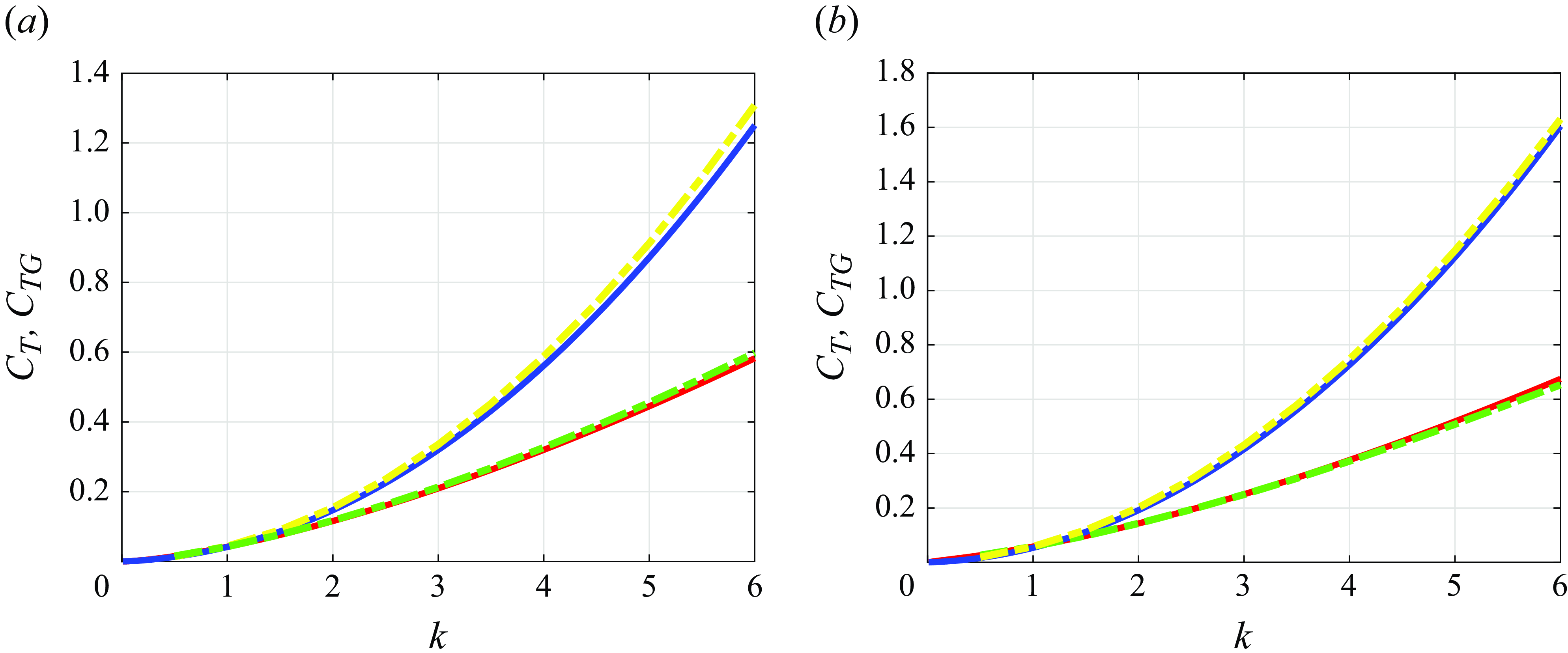
Figure 8. (a) Comparison between the values of $C_T(k)$
and of
$C_T(k)$
and of $C_{TG}(k)$
for an airfoil in purely heaving motion with
$C_{TG}(k)$
for an airfoil in purely heaving motion with ${h_0}/{c}=6\pi /180$
,
${h_0}/{c}=6\pi /180$
, $a_0=0$
. In red, the result of (4.20) and in dashed green the corresponding value obtained numerically using the vortex-lattice method detailed in the supplementary material; in blue, the result of (4.21) and in dashed yellow the corresponding result obtained using the vortex-lattice method detailed in the supplementary material. (b) The same as in (a) but for a combined heaving and pitching motion of the airfoil with
$a_0=0$
. In red, the result of (4.20) and in dashed green the corresponding value obtained numerically using the vortex-lattice method detailed in the supplementary material; in blue, the result of (4.21) and in dashed yellow the corresponding result obtained using the vortex-lattice method detailed in the supplementary material. (b) The same as in (a) but for a combined heaving and pitching motion of the airfoil with $\frac{h_0}{c}=a_0=6\pi /180$
and
$\frac{h_0}{c}=a_0=6\pi /180$
and $\phi =\pi /2$
.
$\phi =\pi /2$
.
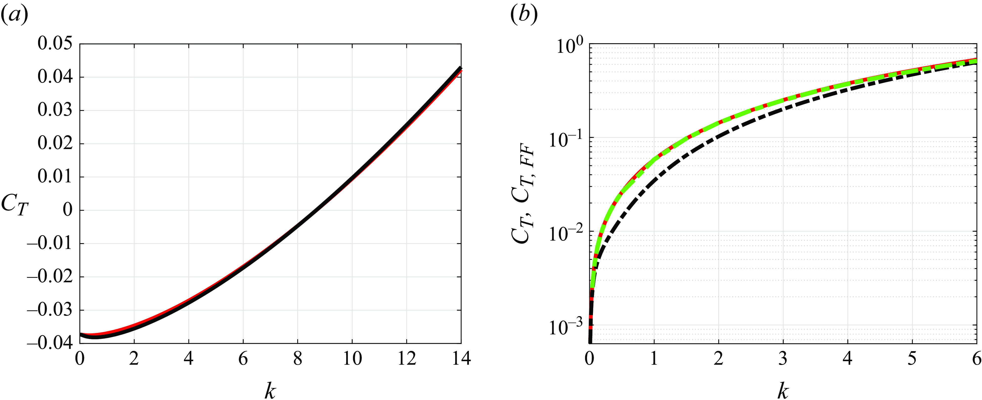
Figure 9. (a) Comparison between the values of $C_{T0} + C_T(k)$
for
$C_{T0} + C_T(k)$
for ${h_0}/{c}=0$
,
${h_0}/{c}=0$
, $a_0=2\pi /180$
and
$a_0=2\pi /180$
and $C_{T0}=-0.0373$
, see Mackowski & Williamson (Reference Mackowski and Williamson2015) and Fernandez-feria (Reference Fernandez-Feria2017), with the thrust coefficient calculated using either (4.20) (red line) or (4.22) (black line). For this particular case, the mean thrust forces predicted by (4.20) and (4.22) are very similar to each other and, therefore, the result in (4.20) is also in good agreement with experiments, as can be inferred from the comparison between the theoretical and experimental results depicted in figure 3(a) of Fernandez-feria (Reference Fernandez-Feria2017). (b) Comparison between the values of the thrust coefficient calculated using either (4.20) (red line) or (4.22) (black dashed line) for
$C_{T0}=-0.0373$
, see Mackowski & Williamson (Reference Mackowski and Williamson2015) and Fernandez-feria (Reference Fernandez-Feria2017), with the thrust coefficient calculated using either (4.20) (red line) or (4.22) (black line). For this particular case, the mean thrust forces predicted by (4.20) and (4.22) are very similar to each other and, therefore, the result in (4.20) is also in good agreement with experiments, as can be inferred from the comparison between the theoretical and experimental results depicted in figure 3(a) of Fernandez-feria (Reference Fernandez-Feria2017). (b) Comparison between the values of the thrust coefficient calculated using either (4.20) (red line) or (4.22) (black dashed line) for ${h_0}/{c}=a_0=6\pi /180$
and
${h_0}/{c}=a_0=6\pi /180$
and $\phi =\pi /2$
. The result obtained using the vortex-lattice numerical code described and provided in the supplementary material, represented using a green dashed line, is practically superimposed to our prediction (in red) given in (4.20).
$\phi =\pi /2$
. The result obtained using the vortex-lattice numerical code described and provided in the supplementary material, represented using a green dashed line, is practically superimposed to our prediction (in red) given in (4.20).
Next, in order to show the differences between (4.20) and (4.22) in a more clear way, figure 9(a) compares the predictions of these two equations for the purely pitching motion of the airfoil ( $\frac{h_0}{c}=0$
) with
$\frac{h_0}{c}=0$
) with $a_0=2\pi /180$
already considered by Mackowski & Williamson (Reference Mackowski and Williamson2015), whereas figure 9(b) compares the values of the mean thrust coefficients given in (4.20) and (4.22) for a case of combined pitching and heaving motions corresponding to
$a_0=2\pi /180$
already considered by Mackowski & Williamson (Reference Mackowski and Williamson2015), whereas figure 9(b) compares the values of the mean thrust coefficients given in (4.20) and (4.22) for a case of combined pitching and heaving motions corresponding to $a_0=\frac{h_0}{c}=6\pi /180$
and
$a_0=\frac{h_0}{c}=6\pi /180$
and $\phi =\pi /2$
. The results in figure 9(a), which incorporate the constant drag coefficient
$\phi =\pi /2$
. The results in figure 9(a), which incorporate the constant drag coefficient $C_{T0}=-0.037$
– see Mackowski & Williamson (Reference Mackowski and Williamson2015), Fernandez-Feria (Reference Fernandez-Feria2017) for details – do not show appreciable differences between (4.20) and (4.22), a fact implying that our (4.20) is also in good agreement with the experiments reported by Mackowski & Williamson (Reference Mackowski and Williamson2015) – see figure 3(a) in Fernandez-Feria (Reference Fernandez-Feria2017). However, the results depicted in figure 9(b) reveal that the relative differences between the mean thrust coefficients predicted by (4.20) and (4.22) can be as high as
$C_{T0}=-0.037$
– see Mackowski & Williamson (Reference Mackowski and Williamson2015), Fernandez-Feria (Reference Fernandez-Feria2017) for details – do not show appreciable differences between (4.20) and (4.22), a fact implying that our (4.20) is also in good agreement with the experiments reported by Mackowski & Williamson (Reference Mackowski and Williamson2015) – see figure 3(a) in Fernandez-Feria (Reference Fernandez-Feria2017). However, the results depicted in figure 9(b) reveal that the relative differences between the mean thrust coefficients predicted by (4.20) and (4.22) can be as high as $100\%25$
for
$100\%25$
for $k\sim 1$
. In order to decipher which of the two equations is correct, we have carried out numerical simulations using the vortex-lattice method described and provided in the Supplementary Material. The numerical results, represented using green dashed lines in figure 9(b), are very close to those predicted by our (4.20), a fact indicating that the equation that should be used to predict the mean thrust coefficient when the airfoil oscillates periodically, the contribution of the starting vortex is zero and the vortices in the wake are convected with the free-stream velocity and, hence, the vortex force term (2.40) is negligible, is (4.20), which differs from the one deduced by Fernandez-Feria (Reference Fernandez-Feria2016).
$k\sim 1$
. In order to decipher which of the two equations is correct, we have carried out numerical simulations using the vortex-lattice method described and provided in the Supplementary Material. The numerical results, represented using green dashed lines in figure 9(b), are very close to those predicted by our (4.20), a fact indicating that the equation that should be used to predict the mean thrust coefficient when the airfoil oscillates periodically, the contribution of the starting vortex is zero and the vortices in the wake are convected with the free-stream velocity and, hence, the vortex force term (2.40) is negligible, is (4.20), which differs from the one deduced by Fernandez-Feria (Reference Fernandez-Feria2016).
However, for those cases in which the experiments or the numerical simulations do not violate the starting hypotheses of the potential flow linearised theory, the mean thrust coefficient should be calculated using the original, self-consistent, results of Garrick, reproduced in (4.21) using our variables. Notice, finally, that, if a particular experiment or numerical simulation is such that the contribution to the thrust of the wake vortices cannot be neglected but the development of nonlinearities makes the contribution of the starting vortex to thrust negligible, then, the expression that should be used to predict mean thrust coefficient would be
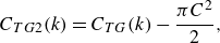 \begin{equation} C_{TG2}(k)=C_{TG}(k)- \frac{\pi C^2}{2}, \end{equation}
with the value of $C$
given in Appendix A and with
$C$
given in Appendix A and with $C_{TG}(k)$
given in (4.21). It could also happen that a particular experiment or numerical simulation is such that the contribution to thrust of the wake vortices is negligible because these vortices are convected with the incident velocity, but the contribution of the starting vortex to thrust cannot be neglected. In this latter case, the mean thrust coefficient would be given by
$C_{TG}(k)$
given in (4.21). It could also happen that a particular experiment or numerical simulation is such that the contribution to thrust of the wake vortices is negligible because these vortices are convected with the incident velocity, but the contribution of the starting vortex to thrust cannot be neglected. In this latter case, the mean thrust coefficient would be given by
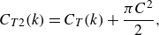 \begin{equation} C_{T2}(k)=C_{T}(k) + \frac{\pi C^2}{2}, \end{equation}
with the values of $C_T(k)$
and
$C_T(k)$
and $C$
given, respectively, by (4.20) and (A4). Clearly, the most appropriate equation to predict the mean thrust coefficient through (4.20), (4.21), (4.23) or (4.24), will depend on the type of nonlinearities developing both in the wake and in the starting vortex and also on the Reynolds number. Consequently, the predictions deduced here using the linearised potential flow theory should be checked against detailed numerical calculations carried out at finite but high Reynolds numbers; as it was pointed out above, this additional task exceeds the limits of the present contribution.
$C$
given, respectively, by (4.20) and (A4). Clearly, the most appropriate equation to predict the mean thrust coefficient through (4.20), (4.21), (4.23) or (4.24), will depend on the type of nonlinearities developing both in the wake and in the starting vortex and also on the Reynolds number. Consequently, the predictions deduced here using the linearised potential flow theory should be checked against detailed numerical calculations carried out at finite but high Reynolds numbers; as it was pointed out above, this additional task exceeds the limits of the present contribution.
5. Conclusions
Here, we have deduced equations for the value of the time-varying thrust as a function of the vorticity distribution along the airfoil and the wake. Moreover, we have shown that these equations reproduce the classical expression for the thrust deduced by Garrick (Reference Garrick1936) once the vertical component of the wake velocity is calculated as a result of the velocities induced by the vortex sheet extending along the airfoil and the wake and the contribution of the flux of horizontal momentum induced by the starting vortex, which cannot be neglected in those cases in which the airfoil is suddenly set into motion, is taken into account. We have also discussed the conditions under which Garrick’s theory is valid and, hence, can be safely used to predict experimental or numerical results. The reasons behind the ability of other results in the literature to approximate the experimental measurements better than Garrick’s theory have also been discussed and we have deduced the equation for the transient thrust force experienced by airfoils suddenly set into motion. Moreover, for those cases in which the airfoil oscillates periodically, the flux of horizontal momentum induced by the starting vortex is negligible and the vortices in the wake are convected downstream at the free-stream velocity, we have deduced an equation for the mean thrust coefficient which differs from the analogous equation in Fernandez-Feria (Reference Fernandez-Feria2016). Our equation for the mean thrust, which has been validated by comparing the theoretical predictions with the numerical results obtained using the vortex-lattice method, is also in good agreement with previously reported experimental data and with nonlinear numerical simulations. We have verified all the analytical results derived in this study using the vortex-lattice method detailed in the Supplementary Material.
Supplementary material.
Supplementary material is available at https://doi.org/10.1017/jfm.2025.10177.
Acknowledgements.
I wish to thank Professor G. Riboux for drawing the sketch in figure 1 and to Dr I. Angulo for pointing out, once the manuscript was finished, that a special case of (3.13) was included on page 705 of Donovan & Lawrence (Reference Donovan and Lawrence1957).
Declaration of interests.
The author reports no conflict of interest
Appendix A
The value of $C$
in (2.27) results from the solution of the integral equation (2.16) particularised at
$C$
in (2.27) results from the solution of the integral equation (2.16) particularised at $t=0^ + $
. This solution must satisfy both the Kutta condition and the Bjerness–Kelvin theorem i.e.
$t=0^ + $
. This solution must satisfy both the Kutta condition and the Bjerness–Kelvin theorem i.e. $\gamma _a(x\rightarrow c,t=0^ + )$
is finite at the trailing edge of the airfoil and
$\gamma _a(x\rightarrow c,t=0^ + )$
is finite at the trailing edge of the airfoil and $\Gamma _a(x\rightarrow c,t=0^ + )=0$
. Notice first that, for purely heaving motions of the airfoil i.e.
$\Gamma _a(x\rightarrow c,t=0^ + )=0$
. Notice first that, for purely heaving motions of the airfoil i.e. $\dot {\alpha }_0=0$
, with the subscript 0 denoting here the value of a variable particularised at the instant
$\dot {\alpha }_0=0$
, with the subscript 0 denoting here the value of a variable particularised at the instant $t=0^ + $
, the non-circulatory solution of (2.16) implies that the flow must be symmetric with respect to
$t=0^ + $
, the non-circulatory solution of (2.16) implies that the flow must be symmetric with respect to $x=c/2$
. This solution is analogous to the one corresponding to a potential flow around a plate of length
$x=c/2$
. This solution is analogous to the one corresponding to a potential flow around a plate of length $a(t)=c + U_\infty t$
at angle of incidence of
$a(t)=c + U_\infty t$
at angle of incidence of $\pi /2$
and, consequently,
$\pi /2$
and, consequently,
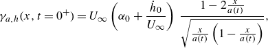 \begin{equation} \gamma_{a,h}(x,t=0^+)=U_\infty\left(\alpha_0+\frac{\dot{h}_0}{U_\infty}\right)\,\frac{1-2\frac{x}{a(t)}}{\sqrt{\frac{x}{a(t)}\left(1-\frac{x}{a(t)}\right)}} , \end{equation}
where the subscript $h$
indicates heaving motion and
$h$
indicates heaving motion and $a(t)=c + U_\infty t$
. Indeed, notice that the circulation density in (A1) expresses that infinite velocities are attained at both the leading edge and at the starting vortex, as is dictated by (2.17) and (2.27), but not at the trailing edge,
$a(t)=c + U_\infty t$
. Indeed, notice that the circulation density in (A1) expresses that infinite velocities are attained at both the leading edge and at the starting vortex, as is dictated by (2.17) and (2.27), but not at the trailing edge, $x=c$
. For the case in which
$x=c$
. For the case in which $\dot {\alpha }_0\neq 0$
, notice that
$\dot {\alpha }_0\neq 0$
, notice that $\dot {\alpha }_0 (x-x_e )=\dot {\alpha }_0 (x-3c/4 ) + \dot {\alpha }_0 (3c/4-x_e )$
and, hence, since the second term corresponds to a uniform vertical velocity along the airfoil, like in a purely heaving motion, we make use of the result in (A1) to conclude that the solution of (2.16) at
$\dot {\alpha }_0 (x-x_e )=\dot {\alpha }_0 (x-3c/4 ) + \dot {\alpha }_0 (3c/4-x_e )$
and, hence, since the second term corresponds to a uniform vertical velocity along the airfoil, like in a purely heaving motion, we make use of the result in (A1) to conclude that the solution of (2.16) at $t=0^ + $
corresponding to arbitrary heaving and pitching motions is
$t=0^ + $
corresponding to arbitrary heaving and pitching motions is
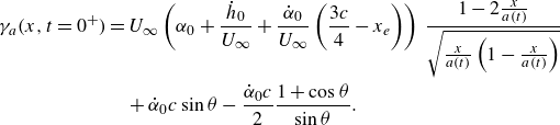 \begin{align}\begin{split}\gamma_{a}(x,t=0^+)&=U_\infty\left(\alpha_0+\frac{\dot{h}_0}{U_\infty}+\frac{\dot{\alpha}_0}{U_\infty}\left(\frac{3c}{4}-x_e\right)\right)\,\frac{1-2 \frac{x}{a(t)}}{\sqrt{\frac{x}{a(t)}\left(1-\frac{x}{a(t)}\right)}}\\& \quad +\dot{\alpha}_0 c\sin\theta-\frac{\dot{\alpha}_0 c}{2}\frac{1+\cos\theta}{\sin\theta} .\end{split}\end{align}
In (A2) we have made use of Glauert’s method, see (2.19) and (2.20), in order to find that the non-circulatory solution of the integral equation (2.16) corresponding to $w'_a(x,t=0^ + )=-\dot {\alpha }_0 (x-3c/4 )$
with
$w'_a(x,t=0^ + )=-\dot {\alpha }_0 (x-3c/4 )$
with $\gamma _a(x,c)=0$
is
$\gamma _a(x,c)=0$
is
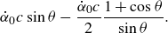 \begin{equation} \dot {\alpha }_0 c\sin \theta -\frac {\dot {\alpha }_0 c}{2}\frac {1 + \cos \theta }{\sin \theta } . \end{equation}
Hence, (2.27) and (A2) indicate that
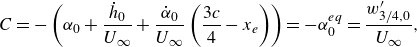 \begin{equation} C=-\left (\alpha _0 + \frac {\dot {h}_0}{U_\infty } + \frac {\dot {\alpha }_0}{U_\infty }\left (\frac {3c}{4}-x_e\right )\right )=-\alpha ^{eq}_0=\frac {w'_{3/4,0}}{U_\infty } , \end{equation}
with $w'_{3/4}$
the value of the perturbed vertical velocity at
$w'_{3/4}$
the value of the perturbed vertical velocity at $x=3/4c$
. The result in (A4) reveals that the contribution to the thrust force of the flux of horizontal momentum induced by the starting vortex cannot be neglected when the airfoil is suddenly set into motion. Let us finally point out that we show in the Supplementary Material that the value of the lift force calculated at
$x=3/4c$
. The result in (A4) reveals that the contribution to the thrust force of the flux of horizontal momentum induced by the starting vortex cannot be neglected when the airfoil is suddenly set into motion. Let us finally point out that we show in the Supplementary Material that the value of the lift force calculated at $t=0^ + $
using the density of circulation given by (A2) recovers the value of the circulatory lift calculated by Wagner at this instant of time.
$t=0^ + $
using the density of circulation given by (A2) recovers the value of the circulatory lift calculated by Wagner at this instant of time.
Appendix B
It is the purpose in this appendix to express the vortex thrust force of the vortices on the airfoil, given by the third term in (2.37), namely,
 \begin{equation} -\rho \int _0^c w'_a\,\gamma _a\,{\rm d}x ,\end{equation}
as a function of $\gamma _w(x,t)$
. First, notice that the substitution of (2.1) into (2.4) yields
$\gamma _w(x,t)$
. First, notice that the substitution of (2.1) into (2.4) yields
 \begin{equation} w'_{a}(x,z=0^\pm ,t)=\frac {\partial z_{a}}{\partial t} + U_\infty \frac {\partial z_{a}}{\partial x}=-\dot {h}-U_\infty \alpha -\dot {\alpha }\left (x-\frac {c}{2}-a\frac {c}{2}\right ) ,\end{equation}
with dots denoting time derivatives and where we have taken into account that $x_e=c/2 + a (c/2 )=c/2 + x_c$
. Moreover, we make use of the idea in von Kármán & Sears (Reference von Kármán and Sears1938) of expressing the density of circulation at the airfoil as
$x_e=c/2 + a (c/2 )=c/2 + x_c$
. Moreover, we make use of the idea in von Kármán & Sears (Reference von Kármán and Sears1938) of expressing the density of circulation at the airfoil as
 \begin{equation} \gamma _a(x,t)=\gamma _0(x,t) + \gamma _1(x,t) , \end{equation}
with $\gamma _0(x,t)$
the circulation density satisfying the impenetrability condition expressed by (B2) along
$\gamma _0(x,t)$
the circulation density satisfying the impenetrability condition expressed by (B2) along $0\leqslant x\leqslant c$
if the wake had no effect and
$0\leqslant x\leqslant c$
if the wake had no effect and $\gamma _1(x,t)$
is the circulation density induced in the airfoil by the vortices in the wake, namely, it is a circulation density such that the vertical velocity field induced by
$\gamma _1(x,t)$
is the circulation density induced in the airfoil by the vortices in the wake, namely, it is a circulation density such that the vertical velocity field induced by $\gamma _1(x,t)$
plus the vertical velocity field induced by the vortices in the wake is zero along
$\gamma _1(x,t)$
plus the vertical velocity field induced by the vortices in the wake is zero along $0\leqslant x \leqslant c$
. The value of
$0\leqslant x \leqslant c$
. The value of $\gamma _0(x,t)$
, which was also called quasi-steady vorticity distribution by von Kármán & Sears (Reference von Kármán and Sears1938), can be straightforwardly calculated using Glauert’s method to give
$\gamma _0(x,t)$
, which was also called quasi-steady vorticity distribution by von Kármán & Sears (Reference von Kármán and Sears1938), can be straightforwardly calculated using Glauert’s method to give
 \begin{equation} \gamma _0(x,t)=2\left [\left (\dot {h} + U_\infty \alpha -x_c\dot {\alpha }\right )\tan (\psi /2) + \dot {\alpha }c/2\sin \psi \right ]\quad \mathrm{with}\quad x/c= \frac{(1 + \cos \psi )}{2} , \end{equation}
whereas, following the result in equations (13) and (14) in von Kármán & Sears (Reference von Kármán and Sears1938), $\gamma _1(x,t)$
is related with
$\gamma _1(x,t)$
is related with $\gamma _w(x,t)$
through the equation
$\gamma _w(x,t)$
through the equation
 \begin{equation} \int _{-1}^{1} \chi \gamma _1(\chi ,t)\,{\rm d}\chi =\int _1^{1 + 2U_\infty t/c} \gamma _w(\chi ,t)\left (\sqrt {\chi ^2-1}-\chi \right )\,{\rm d}\chi \quad \mathrm{with}\quad \chi =\frac {x-\dfrac{c}{2}}{\dfrac{c}{2}} . \end{equation}
The substitution of (B2) and (B3) into (B1) yields
 \begin{equation} -\rho \int _0^c w'_a\,\gamma _a\,{\rm d}x=-\rho \int _0^c\left (\gamma _0 + \gamma _1\right )\left [-\dot {h}-U_\infty \alpha -\dot {\alpha }\left (x-\frac {c}{2}-a\frac {c}{2}\right )\right ]\,{\rm d}x . \end{equation}
Finally, making use of the Bjerness–Kelvin theorem, which expresses that the total circulation around the airfoil and the wake must be zero and, consequently, implies that
 \begin{equation} \int _0^c\left (\gamma _0 + \gamma _1\right )\,{\rm d}x=-\int _c^{c + U_\infty t} \gamma _w {\rm d}x ,\end{equation}
we find, after substitution of (B4) and (B5) into (B6) that, for $t\gt 0$
,
$t\gt 0$
,
 \begin{align} &-\rho \int _0^c w'_a\,\gamma _a\,{\rm d}x=\frac {\rho \pi \,c^2\dot {\alpha }}{4}\left (-\dot {h}-U_\infty \alpha + x_c\,\dot {\alpha }\right )\notag\\& + \rho \frac {c}{2}\int _1^{1 + 2U_\infty t/c}\left [-\dot {h}-U_\infty \alpha + x_c\dot {\alpha } + \left (\frac{c}{2}\right )\dot {\alpha }\left (\sqrt {\chi ^2-1}-\chi \right )\right ]\gamma _w(\chi ,t)\,{\rm d}\chi , \end{align}
where we have taken into account that $x_c=a (c/2 )$
. Notice that, right at
$x_c=a (c/2 )$
. Notice that, right at $t=0^ + $
,
$t=0^ + $
, $\gamma _0(x,t=0^ + )$
is given by
$\gamma _0(x,t=0^ + )$
is given by $\gamma _a(x,t=0^ + )$
in (A1) instead of by (B4), but the result in (B8) in the limit
$\gamma _a(x,t=0^ + )$
in (A1) instead of by (B4), but the result in (B8) in the limit $t\rightarrow 0^ + $
is still valid because
$t\rightarrow 0^ + $
is still valid because
 \begin{equation} \rho \dot {\alpha }\int _0^c \left (x-\frac {c}{2}\right )\gamma _{a}(x,t=0^ + )\,{\rm d}x=\frac {\rho \pi \,c^2\dot {\alpha }}{4}\left (-\dot {h}-U_\infty \alpha + x_c\,\dot {\alpha }\right ) . \end{equation}
Finally, notice that the results in this appendix also reveal that the reason why the thrust vortex force in (B1) depends on the circulation density $\gamma _w$
, see (B8), is because the density of circulation on the airfoil,
$\gamma _w$
, see (B8), is because the density of circulation on the airfoil, $\gamma _a$
, depends on the vertical velocities induced by the vortices in the wake through the circulation density
$\gamma _a$
, depends on the vertical velocities induced by the vortices in the wake through the circulation density $\gamma _1$
in (B3). The indirect dependence on
$\gamma _1$
in (B3). The indirect dependence on $\gamma _w$
of the vortex thrust force of the vortices on the airfoil in (B1) should not be confused with the vortex thrust force of the vortices in the wake expressed by (2.40), a term which is missing in Fernandez-Feria (Reference Fernandez-Feria2016, Reference Fernandez-Feria2017), Alaminos-Quesada & Fernandez-Feria (Reference Alaminos-Quesada and Fernandez-Feria2020) and Sanchez-Laulhe et al. (Reference Sanchez-Laulhe, Fernandez-Feria and Ollero2023), see (2.38) and the discussion below.
$\gamma _w$
of the vortex thrust force of the vortices on the airfoil in (B1) should not be confused with the vortex thrust force of the vortices in the wake expressed by (2.40), a term which is missing in Fernandez-Feria (Reference Fernandez-Feria2016, Reference Fernandez-Feria2017), Alaminos-Quesada & Fernandez-Feria (Reference Alaminos-Quesada and Fernandez-Feria2020) and Sanchez-Laulhe et al. (Reference Sanchez-Laulhe, Fernandez-Feria and Ollero2023), see (2.38) and the discussion below.


 Open access