


1. Introduction
Flow-induced vibrations (FIV) of bluff bodies are encountered in a myriad of physical systems, from the oscillations of plants in wind to those of mooring lines and risers exposed to ocean currents in offshore industry. The impact of FIV on the fatigue life of engineering structures, as well as their fundamental interest as paradigms of fluid–structure interaction, have stimulated an intense research activity, as reviewed, for example, by Blevins (Reference Blevins1990), Païdoussis et al. (Reference Païdoussis, Price and de Langre2010) and Modarres-Sadeghi (Reference Modarres-Sadeghi2022).
A circular cylinder placed in a cross-current is susceptible to vortex-induced vibrations (VIV), a form of FIV driven by the synchronisation, or lock-in, between body motion and flow unsteadiness associated with vortex formation in the wake (Williamson & Govardhan Reference Williamson and Govardhan2004). The configuration composed of a cylinder, placed in a uniform oncoming flow normal to its axis, and free to translate along a rectilinear path, i.e. with a single degree of freedom, represents a canonical problem to investigate these vibrations (Feng Reference Feng1968; Mittal & Tezduyar Reference Mittal and Tezduyar1992; Hover et al. Reference Hover, Techet and Triantafyllou1998; Khalak & Williamson Reference Khalak and Williamson1999; Klamo et al. Reference Klamo, Leonard and Roshko2006; Leontini et al. Reference Leontini, Stewart, Thompson and Hourigan2006; Naudascher Reference Naudascher1987; Cagney & Balabani Reference Cagney and Balabani2013; Konstantinidis Reference Konstantinidis2014; Riches & Morton Reference Riches and Morton2018; Bourguet Reference Bourguet2019; Gurian et al. Reference Gurian, Currier and Modarres-Sadeghi2019; Benner & Modarres-Sadeghi Reference Benner and Modarres-Sadeghi2021; Konstantinidis et al. Reference Konstantinidis, Dorogi and Baranyi2021). In nature and in industrial systems, VIV often arise in the presence of a structural restoring force (SRF), and thus of a structural natural frequency. This is also the case in the above-mentioned studies, where the cylinder was usually mounted on an elastic support. The typical peak amplitudes of vibration vary with the orientation of the direction of motion, called incidence hereafter and defined by the angle $\theta$
relative to the oncoming flow: of the order of one body diameter at normal incidence (
$\theta$
relative to the oncoming flow: of the order of one body diameter at normal incidence ( $\theta =90^\circ$
), the amplitude tends to decrease as
$\theta =90^\circ$
), the amplitude tends to decrease as $\theta$
is reduced, to become one or more orders of magnitude lower when the motion is aligned with the oncoming flow (
$\theta$
is reduced, to become one or more orders of magnitude lower when the motion is aligned with the oncoming flow ( $\theta =0^\circ$
). Once body oscillation and flow unsteadiness are synchronised, the vibration frequency can depart from the natural frequency associated with the SRF, but also from the vortex shedding frequency downstream of a rigidly mounted cylinder (Strouhal frequency). The organisation of the flow (its symmetry properties, the number of vortices shed per period) can considerably differ from the von Kármán vortex street developing in the rigidly mounted body wake.
$\theta =0^\circ$
). Once body oscillation and flow unsteadiness are synchronised, the vibration frequency can depart from the natural frequency associated with the SRF, but also from the vortex shedding frequency downstream of a rigidly mounted cylinder (Strouhal frequency). The organisation of the flow (its symmetry properties, the number of vortices shed per period) can considerably differ from the von Kármán vortex street developing in the rigidly mounted body wake.
Vortex-induced vibrations also occur in the above canonical configuration when the SRF is removed, i.e. in the absence of structural natural frequency, as shown in prior works for a cylinder free to translate at normal incidence (Shiels et al. Reference Shiels, Leonard and Roshko2001; Govardhan & Williamson Reference Govardhan and Williamson2002; Ryan et al. Reference Ryan, Thompson and Hourigan2005; Navrose & Mittal Reference Mittal2017; Bourguet 2023a). The vibrations arising without SRF only exhibit substantial magnitudes over a narrow range of low values of the structure to displaced fluid mass ratio ( $m^\star$
), typically
$m^\star$
), typically $m^\star \lt 1$
; no such restriction exists with SRF, e.g. Feng (Reference Feng1968) reported large-amplitude responses for a mass ratio close to
$m^\star \lt 1$
; no such restriction exists with SRF, e.g. Feng (Reference Feng1968) reported large-amplitude responses for a mass ratio close to $250$
. Within the low-
$250$
. Within the low- $m^\star$
range, the vibrations without SRF may reach amplitudes comparable to those measured with SRF, but the peak values are generally not attained. The emergence of VIV at Reynolds number (Re) values lower than the critical threshold of
$m^\star$
range, the vibrations without SRF may reach amplitudes comparable to those measured with SRF, but the peak values are generally not attained. The emergence of VIV at Reynolds number (Re) values lower than the critical threshold of $47$
that marks the onset of flow unsteadiness for a rigidly mounted cylinder, was detected down to Re
$47$
that marks the onset of flow unsteadiness for a rigidly mounted cylinder, was detected down to Re $\approx 20$
with SRF (Cossu & Morino Reference Cossu and Morino2000; Mittal & Singh Reference Mittal and Singh2005; Kou et al. Reference Kou, Zhang, Liu and Li2017; Dolci & Carmo Reference Dolci and Carmo2019; Boersma et al. Reference Boersma, Zhao, Rothstein and Modarres-Sadeghi2021; Bourguet 2023b). The Reynolds number is based on the body diameter and oncoming flow velocity. Such subcritical VIV persist without SRF but vibration onset is delayed to Re
$\approx 20$
with SRF (Cossu & Morino Reference Cossu and Morino2000; Mittal & Singh Reference Mittal and Singh2005; Kou et al. Reference Kou, Zhang, Liu and Li2017; Dolci & Carmo Reference Dolci and Carmo2019; Boersma et al. Reference Boersma, Zhao, Rothstein and Modarres-Sadeghi2021; Bourguet 2023b). The Reynolds number is based on the body diameter and oncoming flow velocity. Such subcritical VIV persist without SRF but vibration onset is delayed to Re $\approx 30$
in this case (Ryan et al. Reference Ryan, Thompson and Hourigan2005; Bourguet 2023a). Here and in the following, the terms ‘critical’, ‘subcritical’ and ‘postcritical’ refer to the onset of flow unsteadiness for a rigidly mounted cylinder. The deviation between the responses with and without SRF can be analysed under a harmonic oscillation assumption, which is often acceptable in this context (Govardhan & Williamson Reference Govardhan and Williamson2002). Under this assumption, the responses accessible without SRF correspond to the subset of responses occurring with SRF where the added mass due to fluid forcing is negative. It appears that this subset does not include the peak amplitude vibrations observed with SRF, and that it may even vanish, depending on Re (Bourguet Reference Bourguet2024).
$\approx 30$
in this case (Ryan et al. Reference Ryan, Thompson and Hourigan2005; Bourguet 2023a). Here and in the following, the terms ‘critical’, ‘subcritical’ and ‘postcritical’ refer to the onset of flow unsteadiness for a rigidly mounted cylinder. The deviation between the responses with and without SRF can be analysed under a harmonic oscillation assumption, which is often acceptable in this context (Govardhan & Williamson Reference Govardhan and Williamson2002). Under this assumption, the responses accessible without SRF correspond to the subset of responses occurring with SRF where the added mass due to fluid forcing is negative. It appears that this subset does not include the peak amplitude vibrations observed with SRF, and that it may even vanish, depending on Re (Bourguet Reference Bourguet2024).
The present study widens the investigation of the behaviour of the system without SRF. The incidence angle, restrained to $\theta =90^\circ$
in prior works, is considered as a new parameter of the problem. This breaks the transverse symmetry of the canonical configuration. In addition, a second form of symmetry breaking is introduced, via a forced rotation of the cylinder about its axis. The rotation rate
$\theta =90^\circ$
in prior works, is considered as a new parameter of the problem. This breaks the transverse symmetry of the canonical configuration. In addition, a second form of symmetry breaking is introduced, via a forced rotation of the cylinder about its axis. The rotation rate $\alpha$
, defined as the ratio between cylinder surface and oncoming flow velocities, is also considered as a parameter. The effects of a forced rotation, such as the appearance of a time-averaged fluid force normal to the oncoming flow (Magnus effect) and the disruption of the two- and three-dimensional transition scenario of the flow as a function of the Reynolds number, have been well documented for a rigidly mounted cylinder (Coutanceau & Ménard Reference Coutanceau and Ménard1985; Kang et al. Reference Kang, Choi and Lee1999; Stojković et al. Reference Stojković, Breuer and Durst2002; Mittal & Kumar Reference Mittal and Kumar2003; Pralits et al. Reference Pralits, Brandt and Giannetti2010; Navrose et al. Reference Navrose and Mittal2015; Rao et al. Reference Rao, Radi, Leontini, Thompson, Sheridan and Hourigan2015). The introduction of a forced rotation in the present system was motivated by its reported influence on the FIV of a cylinder with SRF (Stansby & Rainey Reference Stansby and Rainey2001; Yogeswaran & Mittal Reference Yogeswaran and Mittal2011; Bourguet & Lo Jacono Reference Bourguet and Lo Jacono2014; Zhao et al. Reference Zhao, Cheng and Lu2014; Seyed-Aghazadeh & Modarres-Sadeghi Reference Seyed-Aghazadeh and Modarres-Sadeghi2015; Wong et al. Reference Wong, Zhao, Lo Jacono, Thompson and Sheridan2017; Bourguet Reference Bourguet2019, Reference Bourguet2020, Reference Bourguet2023b
; Munir et al. Reference Munir, Zhao, Wu and Tong2021; Zhao et al. Reference Zhao, Thompson and Hourigan2022). Among other aspects, the rotation was found to modify the threshold value of the Reynolds number where vibrations arise, and expand the vibration/flow unsteadiness range from Re
$\alpha$
, defined as the ratio between cylinder surface and oncoming flow velocities, is also considered as a parameter. The effects of a forced rotation, such as the appearance of a time-averaged fluid force normal to the oncoming flow (Magnus effect) and the disruption of the two- and three-dimensional transition scenario of the flow as a function of the Reynolds number, have been well documented for a rigidly mounted cylinder (Coutanceau & Ménard Reference Coutanceau and Ménard1985; Kang et al. Reference Kang, Choi and Lee1999; Stojković et al. Reference Stojković, Breuer and Durst2002; Mittal & Kumar Reference Mittal and Kumar2003; Pralits et al. Reference Pralits, Brandt and Giannetti2010; Navrose et al. Reference Navrose and Mittal2015; Rao et al. Reference Rao, Radi, Leontini, Thompson, Sheridan and Hourigan2015). The introduction of a forced rotation in the present system was motivated by its reported influence on the FIV of a cylinder with SRF (Stansby & Rainey Reference Stansby and Rainey2001; Yogeswaran & Mittal Reference Yogeswaran and Mittal2011; Bourguet & Lo Jacono Reference Bourguet and Lo Jacono2014; Zhao et al. Reference Zhao, Cheng and Lu2014; Seyed-Aghazadeh & Modarres-Sadeghi Reference Seyed-Aghazadeh and Modarres-Sadeghi2015; Wong et al. Reference Wong, Zhao, Lo Jacono, Thompson and Sheridan2017; Bourguet Reference Bourguet2019, Reference Bourguet2020, Reference Bourguet2023b
; Munir et al. Reference Munir, Zhao, Wu and Tong2021; Zhao et al. Reference Zhao, Thompson and Hourigan2022). Among other aspects, the rotation was found to modify the threshold value of the Reynolds number where vibrations arise, and expand the vibration/flow unsteadiness range from Re $\approx 20$
in the absence of rotation down to Re
$\approx 20$
in the absence of rotation down to Re $\approx 4$
at high rotation rates. The rotation may lead to a major amplification of body oscillation and trigger a transition from VIV to another form of response, referred to as galloping-like, whose magnitude increases unboundedly as the structural natural frequency is reduced, contrary to VIV. Here, the impact of a forced rotation and associated symmetry breaking are examined for the system without SRF.
$\approx 4$
at high rotation rates. The rotation may lead to a major amplification of body oscillation and trigger a transition from VIV to another form of response, referred to as galloping-like, whose magnitude increases unboundedly as the structural natural frequency is reduced, contrary to VIV. Here, the impact of a forced rotation and associated symmetry breaking are examined for the system without SRF.
Without SRF, when the direction of motion departs from the normal incidence or due to the imposed rotation, i.e. when the transverse symmetry of the system is broken, the body may drift along the rectilinear path. The conditions associated with the flow seen by the drifting cylinder deviate from the nominal conditions based on the oncoming flow ( $\theta$
, Re and
$\theta$
, Re and $\alpha$
). For example, the body may be exposed to subcritical conditions even though the nominal conditions in terms of Re and
$\alpha$
). For example, the body may be exposed to subcritical conditions even though the nominal conditions in terms of Re and $\alpha$
are far from the critical values. The drift needs to be quantified, in particular, to delimit the actual parameter space visited by the system, relative to the nominal conditions. The possible combination of the drifting motion with an oscillation of the body poses the question of the validity of a quasi-steady approach to predict it.
$\alpha$
are far from the critical values. The drift needs to be quantified, in particular, to delimit the actual parameter space visited by the system, relative to the nominal conditions. The possible combination of the drifting motion with an oscillation of the body poses the question of the validity of a quasi-steady approach to predict it.
The incidence angle and the rotation rate are introduced as parameters of the problem and the parameter space includes the reference configuration studied in previous works concerning the system without SRF, $\theta =90^\circ$
and
$\theta =90^\circ$
and $\alpha =0$
. The VIV identified in this case are expected to persist, at least over a portion of the present parameter space. Some insights into the alteration of these vibrations can be gained from the results obtained with SRF. The frequency of the peak amplitude vibrations observed with SRF, in the absence of rotation, tends to decrease as the incidence angle is reduced from
$\alpha =0$
. The VIV identified in this case are expected to persist, at least over a portion of the present parameter space. Some insights into the alteration of these vibrations can be gained from the results obtained with SRF. The frequency of the peak amplitude vibrations observed with SRF, in the absence of rotation, tends to decrease as the incidence angle is reduced from $90^\circ$
(Bourguet Reference Bourguet2019). This suggests an increase of the added mass and thus, under the harmonic oscillation assumption, a reduction of the large-amplitude response range accessible without SRF. This mechanism combines with the general decrease of the peak amplitudes reported with SRF when the incidence angle is reduced (Brika & Laneville Reference Brika and Laneville1995; Benner & Modarres-Sadeghi Reference Benner and Modarres-Sadeghi2021). Therefore, a reduction of the incidence angle could lead to lower VIV amplitudes for the present system. A comparable decreasing evolution of the vibration frequency can be noted, at normal incidence, when the rotation rate is increased (Bourguet & Lo Jacono Reference Bourguet and Lo Jacono2014). Yet, the effect of the rotation on the added mass could be counterbalanced by the simultaneous amplification of the vibration, and no clear trend can be conjectured concerning the influence of the rotation. Beyond VIV, the possible emergence of distinct forms of structural response due to the imposed rotation is another point that remains to be clarified, especially for a body drifting at low or no incidence, very close to the oncoming flow velocity, i.e. virtually in the absence of relative current. This aspect links the present problem to the interaction phenomena developing in quiescent fluid.
$90^\circ$
(Bourguet Reference Bourguet2019). This suggests an increase of the added mass and thus, under the harmonic oscillation assumption, a reduction of the large-amplitude response range accessible without SRF. This mechanism combines with the general decrease of the peak amplitudes reported with SRF when the incidence angle is reduced (Brika & Laneville Reference Brika and Laneville1995; Benner & Modarres-Sadeghi Reference Benner and Modarres-Sadeghi2021). Therefore, a reduction of the incidence angle could lead to lower VIV amplitudes for the present system. A comparable decreasing evolution of the vibration frequency can be noted, at normal incidence, when the rotation rate is increased (Bourguet & Lo Jacono Reference Bourguet and Lo Jacono2014). Yet, the effect of the rotation on the added mass could be counterbalanced by the simultaneous amplification of the vibration, and no clear trend can be conjectured concerning the influence of the rotation. Beyond VIV, the possible emergence of distinct forms of structural response due to the imposed rotation is another point that remains to be clarified, especially for a body drifting at low or no incidence, very close to the oncoming flow velocity, i.e. virtually in the absence of relative current. This aspect links the present problem to the interaction phenomena developing in quiescent fluid.
The objective of this paper is to explore the behaviour of the flow–body system when the cylinder, free to translate along a rectilinear path in an arbitrary direction, is subjected to a forced rotation. This generalises prior works on FIV without SRF and may also be regarded as an extension of previous studies concerning rotating cylinders with SRF. In addition, direct connections can be established with the related topic of freely rising or falling objects. The proposed investigation is based on a series of numerical simulations where path orientation is varied from the normal incidence to the oncoming flow direction. It focuses on the low-mass ratio range, $m^\star \in [0.01,1]$
, where the large-amplitude VIV are concentrated in the reference configuration (
$m^\star \in [0.01,1]$
, where the large-amplitude VIV are concentrated in the reference configuration ( $\theta =90^\circ$
,
$\theta =90^\circ$
, $\alpha =0$
). The Reynolds number is set to
$\alpha =0$
). The Reynolds number is set to $100$
, as in several of the above-mentioned studies on cylinder FIV (e.g. Bourguet & Lo Jacono Reference Bourguet and Lo Jacono2014; Bourguet Reference Bourguet2019, Reference Bourguet2020, Reference Bourguet2024). This value of Re, combined with the selected range of rotation rate values,
$100$
, as in several of the above-mentioned studies on cylinder FIV (e.g. Bourguet & Lo Jacono Reference Bourguet and Lo Jacono2014; Bourguet Reference Bourguet2019, Reference Bourguet2020, Reference Bourguet2024). This value of Re, combined with the selected range of rotation rate values, $\alpha \in [0,1]$
, ensures that the flow remains two-dimensional over a wide region of the
$\alpha \in [0,1]$
, ensures that the flow remains two-dimensional over a wide region of the $(\theta ,m^\star ,\alpha )$
parameter space and that the three-dimensional transition, when it occurs, has only a limited influence on the response. This permits precise inspection of the parameter space via two-dimensional simulations. The three-dimensional transition is addressed via dedicated simulations in selected cases.
$(\theta ,m^\star ,\alpha )$
parameter space and that the three-dimensional transition, when it occurs, has only a limited influence on the response. This permits precise inspection of the parameter space via two-dimensional simulations. The three-dimensional transition is addressed via dedicated simulations in selected cases.
The paper is organised as follows. The physical system and the numerical method are presented in § 2. The system behaviour is examined in § 3. The main findings of this work are summarised in § 4.
2. Formulation and numerical method
The flow–body system, its modelling and the parameter space under study are described in § 2.1. The numerical method and its validation are presented in § 2.2.
2.1. Physical system
The physical system is schematised in figure 1. The $(x,y,z)$
frame is fixed. The rigid circular cylinder of diameter
$(x,y,z)$
frame is fixed. The rigid circular cylinder of diameter $D$
and mass per unit length
$D$
and mass per unit length $M_c$
is parallel to the
$M_c$
is parallel to the $z$
axis and placed in an incompressible, uniform oncoming flow of velocity
$z$
axis and placed in an incompressible, uniform oncoming flow of velocity $U \!$
, density
$U \!$
, density $\rho _f$
, viscosity
$\rho _f$
, viscosity $\mu$
and aligned with the
$\mu$
and aligned with the $x$
axis. The physical variables are non-dimensionalised by
$x$
axis. The physical variables are non-dimensionalised by $D$
,
$D$
, $U$
and
$U$
and $\rho _f$
. In the rest of the paper, all the variables are non-dimensional and the term ‘non-dimensional’ is often omitted to simplify the reading. The Reynolds number is defined as Re
$\rho _f$
. In the rest of the paper, all the variables are non-dimensional and the term ‘non-dimensional’ is often omitted to simplify the reading. The Reynolds number is defined as Re $=\rho _f U D/\mu$
. The transition to three-dimensional flow is found to occur within the parameter space investigated. The two-dimensional and three-dimensional Navier–Stokes equations are employed to predict the flow dynamics.
$=\rho _f U D/\mu$
. The transition to three-dimensional flow is found to occur within the parameter space investigated. The two-dimensional and three-dimensional Navier–Stokes equations are employed to predict the flow dynamics.
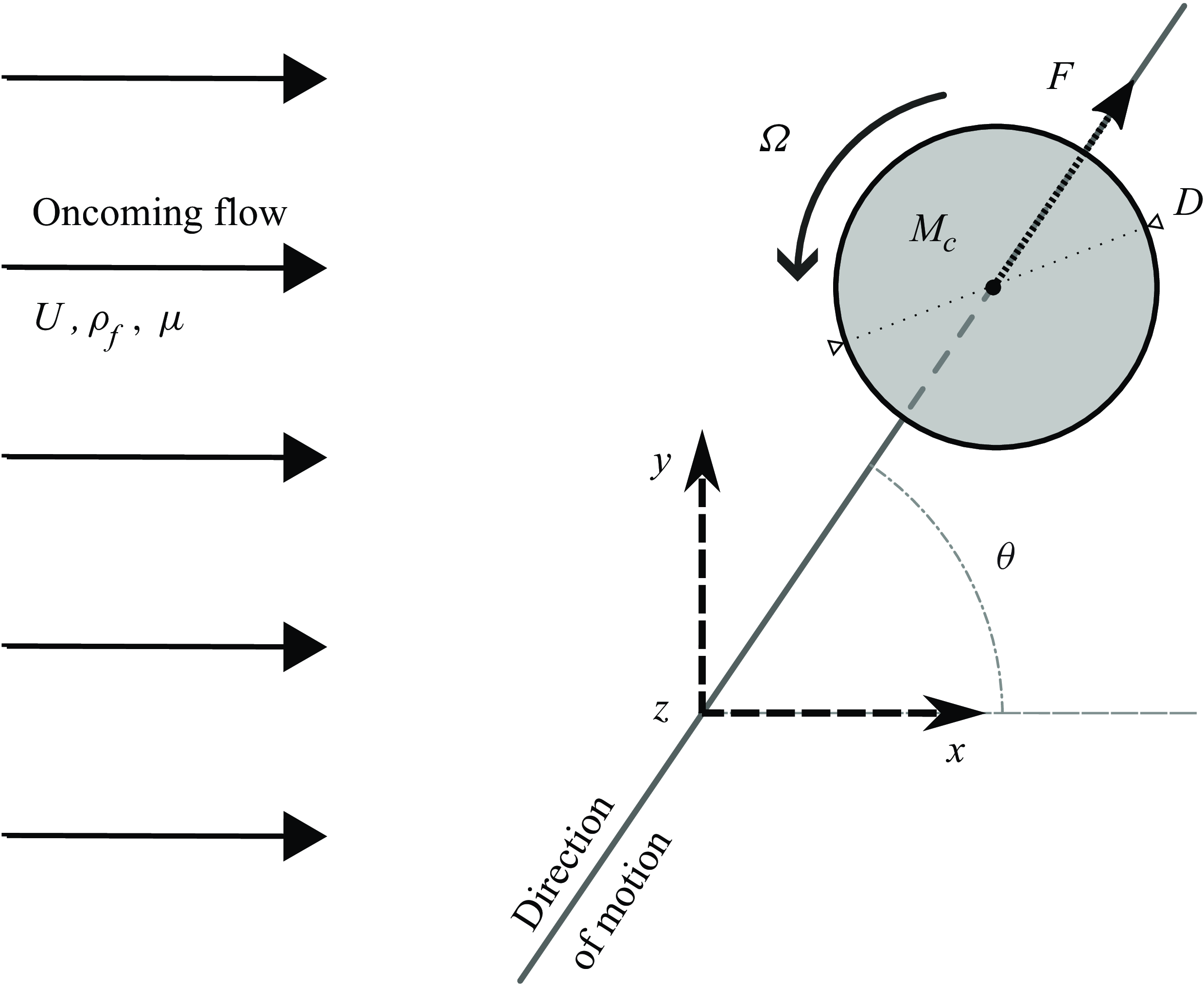
Figure 1. Sketch of the physical system.
The cylinder is free to translate along a rectilinear path, in an arbitrary direction normal to the $z$
axis and defined by the incidence angle
$z$
axis and defined by the incidence angle $\theta$
relative to the
$\theta$
relative to the $x$
axis. The non-dimensional cylinder displacement, velocity and acceleration are denoted by
$x$
axis. The non-dimensional cylinder displacement, velocity and acceleration are denoted by $\zeta$
,
$\zeta$
, $\dot \zeta$
and
$\dot \zeta$
and $\ddot \zeta$
, respectively, where the
$\ddot \zeta$
, respectively, where the $\dot {\phantom {}}$
symbol designates the non-dimensional time derivative. The streamwise, transverse and tangential force coefficients are defined as
$\dot {\phantom {}}$
symbol designates the non-dimensional time derivative. The streamwise, transverse and tangential force coefficients are defined as $C_x=2 F_x /(\rho _f D U^2)$
,
$C_x=2 F_x /(\rho _f D U^2)$
, $C_y=2 F_y /(\rho _f D U^2)$
and
$C_y=2 F_y /(\rho _f D U^2)$
and $C=2 F /(\rho _f D U^2)$
, where
$C=2 F /(\rho _f D U^2)$
, where $F_x$
,
$F_x$
, $F_y$
and
$F_y$
and $F$
are the span-averaged values of the dimensional sectional fluid forces, parallel to the
$F$
are the span-averaged values of the dimensional sectional fluid forces, parallel to the $x$
and
$x$
and $y$
axes, and to the direction of motion, respectively. The tangential force coefficient can be expressed as
$y$
axes, and to the direction of motion, respectively. The tangential force coefficient can be expressed as
 \begin{align} C=C_x \cos \left (\theta \right ) + C_y \sin \left (\theta \right ). \end{align}
The dynamics of the cylinder is governed by the equation
 \begin{align} \ddot {\zeta } = \dfrac {2C}{\pi m^\star }, \end{align}
where the structure to displaced fluid mass ratio is defined as $m^\star = 4 M_c/(\pi \rho _f D^2)$
. The cylinder is subjected to a forced, counter-clockwise, steady rotation about its axis. The rotation is controlled by the rotation rate
$m^\star = 4 M_c/(\pi \rho _f D^2)$
. The cylinder is subjected to a forced, counter-clockwise, steady rotation about its axis. The rotation is controlled by the rotation rate $\alpha = \Omega D / (2U)$
, where
$\alpha = \Omega D / (2U)$
, where $\Omega$
is the angular velocity of the cylinder.
$\Omega$
is the angular velocity of the cylinder.
The Reynolds number is set to $100$
and the behaviour of the flow–body system is explored in the
$100$
and the behaviour of the flow–body system is explored in the $(\theta ,m^\star ,\alpha )$
parameter space, for
$(\theta ,m^\star ,\alpha )$
parameter space, for $m^\star \in [0.01,1]$
and
$m^\star \in [0.01,1]$
and $\alpha \in [0,1]$
. The incidence angles
$\alpha \in [0,1]$
. The incidence angles $\theta$
and
$\theta$
and $\theta +180^\circ$
lead to the same physical configuration. The range
$\theta +180^\circ$
lead to the same physical configuration. The range $\theta \in [0^\circ ,180^\circ ]$
is considered here. In addition, as explained in the Appendix dedicated to the symmetry properties of the system, its behaviour for
$\theta \in [0^\circ ,180^\circ ]$
is considered here. In addition, as explained in the Appendix dedicated to the symmetry properties of the system, its behaviour for $\theta \in [90^\circ ,180^\circ ]$
can be directly deduced from that observed for
$\theta \in [90^\circ ,180^\circ ]$
can be directly deduced from that observed for $\theta \in [0^\circ ,90^\circ ]$
. In the following, the results are thus presented for
$\theta \in [0^\circ ,90^\circ ]$
. In the following, the results are thus presented for $\theta \in [0^\circ ,90^\circ ]$
. The conditions based on the oncoming flow (
$\theta \in [0^\circ ,90^\circ ]$
. The conditions based on the oncoming flow ( $\theta$
,
$\theta$
, ${ Re}$
,
${ Re}$
, $\alpha$
) are referred to as the ‘nominal conditions’, in contrast to the ‘effective conditions’ associated with the flow seen by the drifting cylinder, which will be examined later in the paper.
$\alpha$
) are referred to as the ‘nominal conditions’, in contrast to the ‘effective conditions’ associated with the flow seen by the drifting cylinder, which will be examined later in the paper.
For validation and complementary analyses, a series of simulations is carried out for a rigidly mounted cylinder and for an elastically mounted cylinder. For more clarity in the presentation, the subscripts ${}_r$
and
${}_r$
and ${}_s$
are added to the nominal conditions associated with these systems, (
${}_s$
are added to the nominal conditions associated with these systems, ( ${ Re}_r$
,
${ Re}_r$
, $\alpha _r$
) and (
$\alpha _r$
) and ( $\theta _s$
,
$\theta _s$
, ${ Re}_s$
,
${ Re}_s$
, $\alpha _s$
), respectively. In the latter case, a SRF is introduced by adding the term
$\alpha _s$
), respectively. In the latter case, a SRF is introduced by adding the term $(2\pi f_n)^2\zeta$
on the left-hand side of the dynamics equation (2.2). The corresponding non-dimensional natural frequency and reduced velocity are defined as
$(2\pi f_n)^2\zeta$
on the left-hand side of the dynamics equation (2.2). The corresponding non-dimensional natural frequency and reduced velocity are defined as $f_n=D/(2\pi U)\sqrt {K/M_c}$
and
$f_n=D/(2\pi U)\sqrt {K/M_c}$
and $U^\star =1/f_n$
, where
$U^\star =1/f_n$
, where $K$
is the dimensional stiffness of the elastic support. In the system with SRF, the mass ratio is designated by
$K$
is the dimensional stiffness of the elastic support. In the system with SRF, the mass ratio is designated by $m^\star_{s}$
.
$m^\star_{s}$
.
2.2. Numerical method
The numerical method is the same as in previous studies concerning comparable systems, with and without SRF (Bourguet & Lo Jacono Reference Bourguet and Lo Jacono2014; Bourguet Reference Bourguet2020, Reference Bourguet2023a , Reference Bourguet2024). Descriptions of the simulation approach, boundary conditions and discretisations, as well as detailed validations were reported in these prior works. The method is briefly summarised here and some additional convergence/validation results are presented.
The coupled flow–body equations are solved by the parallelised code Nektar, which is based on the spectral/ $hp$
element method (Karniadakis & Sherwin Reference Karniadakis and Sherwin1999). Body motion is taken into account by adding inertial terms in the Navier–Stokes equations (Newman & Karniadakis Reference Newman and Karniadakis1997). A fictitious mass approach is employed to ensure the numerical stability of the simulation at low mass ratios (Baek & Karniadakis Reference Baek and Karniadakis2012). A large rectangular computational domain is considered in the
$hp$
element method (Karniadakis & Sherwin Reference Karniadakis and Sherwin1999). Body motion is taken into account by adding inertial terms in the Navier–Stokes equations (Newman & Karniadakis Reference Newman and Karniadakis1997). A fictitious mass approach is employed to ensure the numerical stability of the simulation at low mass ratios (Baek & Karniadakis Reference Baek and Karniadakis2012). A large rectangular computational domain is considered in the $(x,y)$
plane (
$(x,y)$
plane ( $350D$
downstream and
$350D$
downstream and $250D$
in front, above and below the cylinder) to avoid any spurious blockage effects due to domain size. This computational domain is discretised in
$250D$
in front, above and below the cylinder) to avoid any spurious blockage effects due to domain size. This computational domain is discretised in $3975$
spectral elements. In the three-dimensional case, the length of the domain along the
$3975$
spectral elements. In the three-dimensional case, the length of the domain along the $z$
axis is set to
$z$
axis is set to $12D$
, which represents a reasonable balance between the spanwise wavelength of the flow pattern, of the order of
$12D$
, which represents a reasonable balance between the spanwise wavelength of the flow pattern, of the order of $1.5D$
, and the numerical cost. A no-slip condition is applied on the body surface and flow periodicity is imposed on the side boundaries.
$1.5D$
, and the numerical cost. A no-slip condition is applied on the body surface and flow periodicity is imposed on the side boundaries.
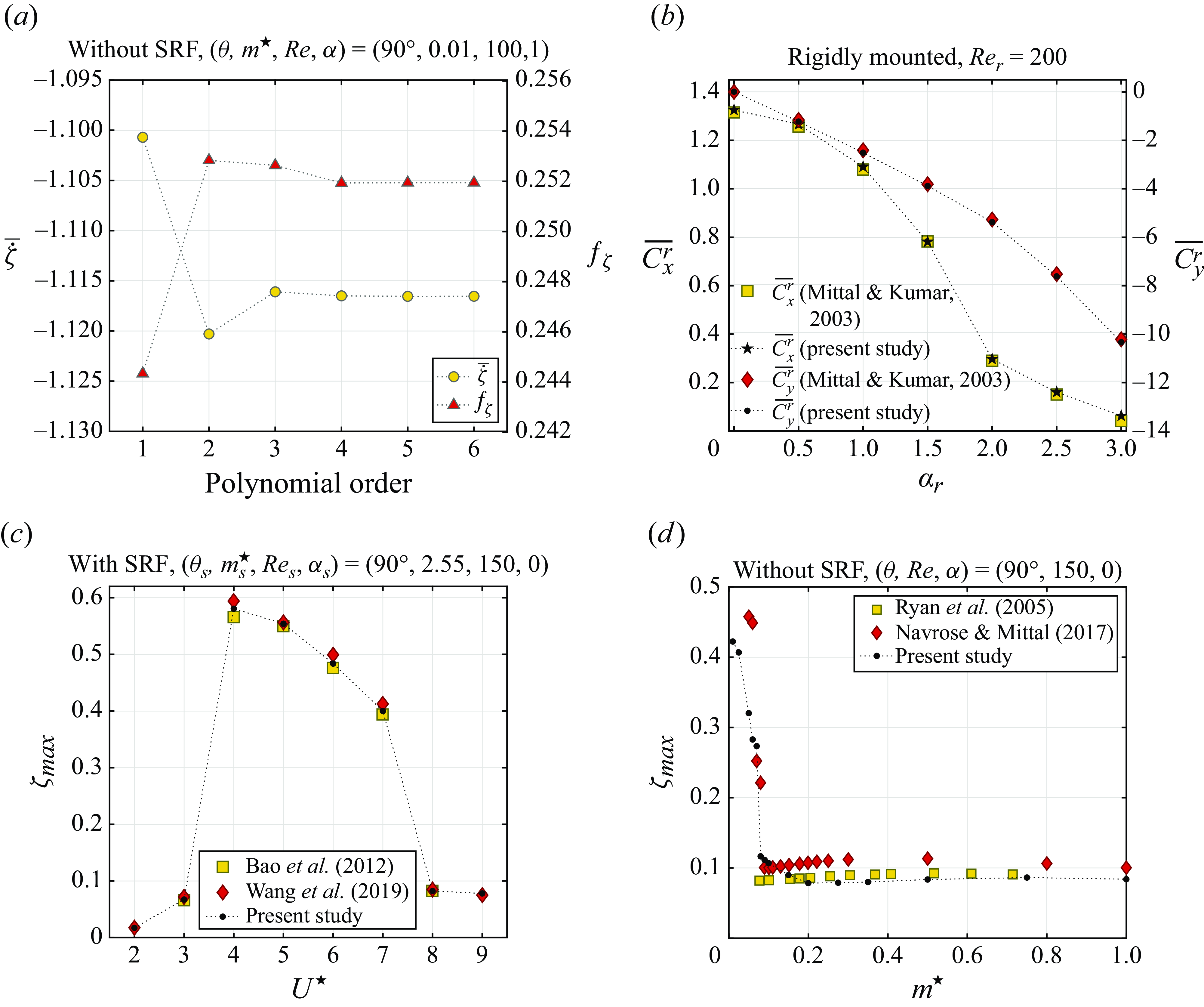
Figure 2. (a) Time-averaged velocity of the cylinder and oscillation frequency as functions of the polynomial order, for $(\theta ,m^\star ,{ Re},\alpha )=(90^\circ ,0.01,100,1)$
. (b) Time-averaged streamwise and transverse force coefficients as functions of the rotation rate, for a rigidly mounted cylinder at
$(\theta ,m^\star ,{ Re},\alpha )=(90^\circ ,0.01,100,1)$
. (b) Time-averaged streamwise and transverse force coefficients as functions of the rotation rate, for a rigidly mounted cylinder at ${ Re}_r=200$
. (c) Oscillation amplitude of an elastically mounted cylinder as a function of the reduced velocity, for
${ Re}_r=200$
. (c) Oscillation amplitude of an elastically mounted cylinder as a function of the reduced velocity, for $(\theta _s,m^\star _s,{ Re}_s,\alpha _s)=(90^\circ ,2.55,150,0)$
. (d) Oscillation amplitude of a cylinder without SRF as a function of the mass ratio, for
$(\theta _s,m^\star _s,{ Re}_s,\alpha _s)=(90^\circ ,2.55,150,0)$
. (d) Oscillation amplitude of a cylinder without SRF as a function of the mass ratio, for $(\theta ,{ Re},\alpha )=(90^\circ ,150,0)$
. The present results are compared to those reported by Mittal & Kumar (Reference Mittal and Kumar2003) in (b), Bao et al. (Reference Bao, Huang, Zhou, Tu and Han2012) and Wang et al. (Reference Wang, Xu, Gao, Liu, Xiao and Ramesh2019) in (c), and Ryan et al. (Reference Ryan, Thompson and Hourigan2005) and Navrose & Mittal (Reference Mittal2017) in (d).
$(\theta ,{ Re},\alpha )=(90^\circ ,150,0)$
. The present results are compared to those reported by Mittal & Kumar (Reference Mittal and Kumar2003) in (b), Bao et al. (Reference Bao, Huang, Zhou, Tu and Han2012) and Wang et al. (Reference Wang, Xu, Gao, Liu, Xiao and Ramesh2019) in (c), and Ryan et al. (Reference Ryan, Thompson and Hourigan2005) and Navrose & Mittal (Reference Mittal2017) in (d).
Figure 2(a) depicts a convergence study in a typical case where the rotating cylinder drifts and oscillates without SRF. This case is located in the region of the parameter space where the Reynolds number based on the relative flow seen by the drifting body reaches its maximum value, close to $160$
. The evolutions of the time-averaged value (denoted by the
$160$
. The evolutions of the time-averaged value (denoted by the $\overline {\phantom {a}}$
symbol) of the cylinder velocity and of its oscillation frequency (
$\overline {\phantom {a}}$
symbol) of the cylinder velocity and of its oscillation frequency ( $f_\zeta$
), as functions of the spectral element polynomial order, show that an increase from order
$f_\zeta$
), as functions of the spectral element polynomial order, show that an increase from order $4$
to
$4$
to $5$
or
$5$
or $6$
has no impact on the results. A polynomial order of
$6$
has no impact on the results. A polynomial order of $4$
was selected. A similar procedure was employed to set the non-dimensional time step, which ranges from
$4$
was selected. A similar procedure was employed to set the non-dimensional time step, which ranges from $0.00125$
to
$0.00125$
to $0.005$
depending on the velocity magnitude of the flow seen by the body. It has also been verified that doubling the number of complex Fourier modes used to discretise the domain along the
$0.005$
depending on the velocity magnitude of the flow seen by the body. It has also been verified that doubling the number of complex Fourier modes used to discretise the domain along the $z$
axis, from
$z$
axis, from $64$
to
$64$
to $128$
, has only a negligible influence on the three-dimensional simulation results.
$128$
, has only a negligible influence on the three-dimensional simulation results.
Three validation studies are proposed in figure 2(b–d). The time-averaged force coefficients for a rigidly mounted rotating cylinder (identified by the superscript ${}^{r}$
) at
${}^{r}$
) at ${ Re}_r=200$
and the oscillation amplitudes of a non-rotating cylinder, free to move at normal incidence with and without SRF, at
${ Re}_r=200$
and the oscillation amplitudes of a non-rotating cylinder, free to move at normal incidence with and without SRF, at ${ Re}_s={ Re}=150$
, are compared with prior simulation results. In these plots, the oscillation amplitude is measured as the maximum value of the displacement signal, denoted by the subscript
${ Re}_s={ Re}=150$
, are compared with prior simulation results. In these plots, the oscillation amplitude is measured as the maximum value of the displacement signal, denoted by the subscript ${}_{max}$
. These comparisons confirm the validity of the present numerical method.
${}_{max}$
. These comparisons confirm the validity of the present numerical method.
The simulations are initialised with the established flow past a stationary cylinder at a Reynolds number equal to $100$
. Then, the forced rotation is started and the body is released. Previous studies on cylinder VIV have shown that the system may exhibit hysteretic behaviours, including without SRF, for example, over narrow
$100$
. Then, the forced rotation is started and the body is released. Previous studies on cylinder VIV have shown that the system may exhibit hysteretic behaviours, including without SRF, for example, over narrow $m^\star$
ranges of typical width close to
$m^\star$
ranges of typical width close to $0.03$
(e.g. Prasanth et al. Reference Prasanth, Premchandran and Mittal2011; Navrose & Mittal Reference Mittal2017). Such behaviours have been detected here by considering distinct initial conditions. However, the principal observations reported in this paper, in particular, concerning the different regimes and their distribution in the parameter space, appear to persist regardless of the initial condition. The hysteresis mechanisms are not further examined in the present work.
$0.03$
(e.g. Prasanth et al. Reference Prasanth, Premchandran and Mittal2011; Navrose & Mittal Reference Mittal2017). Such behaviours have been detected here by considering distinct initial conditions. However, the principal observations reported in this paper, in particular, concerning the different regimes and their distribution in the parameter space, appear to persist regardless of the initial condition. The hysteresis mechanisms are not further examined in the present work.
The entire parameter space is covered by two-dimensional simulations. Three-dimensional simulations are carried out to delimit the region of the parameter space where the flow becomes three-dimensional and to quantify the main properties of this three-dimensionality, as well as its influence on the structural response. The investigation is based on time series collected after the initial transient dies out, over sufficiently long periods, typically more than $40$
oscillation cycles, to ensure convergence of body dynamics and fluid force statistics.
$40$
oscillation cycles, to ensure convergence of body dynamics and fluid force statistics.
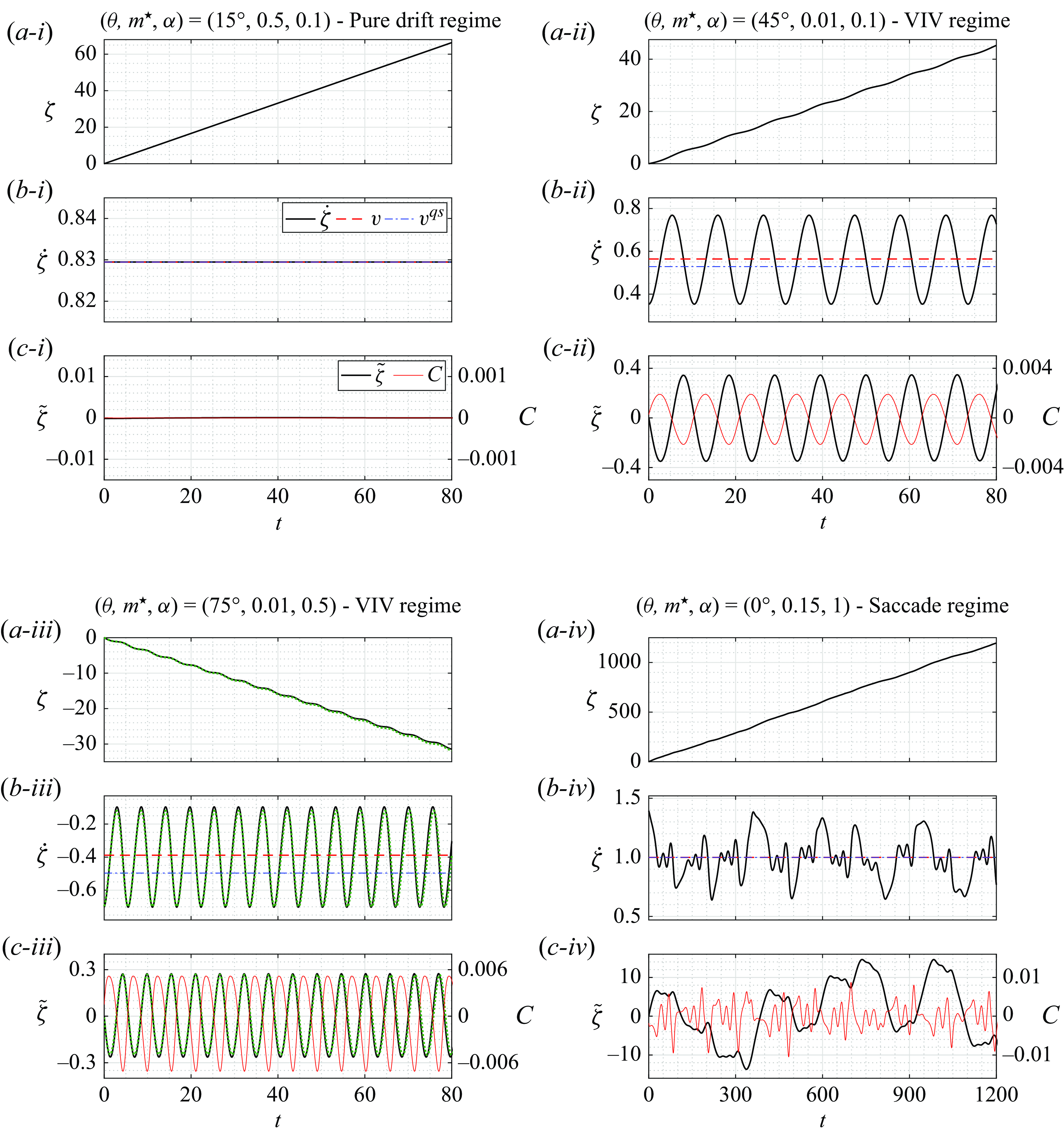
Figure 3. Selected time series of the cylinder (a) displacement, (b) velocity and (c) displacement fluctuation about its linear component, for (i) $(\theta ,m^\star ,\alpha )=(15^\circ ,0.5,0.1)$
(pure drift regime), (ii)
$(\theta ,m^\star ,\alpha )=(15^\circ ,0.5,0.1)$
(pure drift regime), (ii) $(\theta ,m^\star ,\alpha )=(45^\circ ,0.01,0.1)$
(VIV regime), (iii)
$(\theta ,m^\star ,\alpha )=(45^\circ ,0.01,0.1)$
(VIV regime), (iii) $(\theta ,m^\star ,\alpha )=(75^\circ ,0.01,0.5)$
(VIV regime) and (iv)
$(\theta ,m^\star ,\alpha )=(75^\circ ,0.01,0.5)$
(VIV regime) and (iv) $(\theta ,m^\star ,\alpha )=(0^\circ ,0.15,1)$
(saccade regime). The displacement is set to zero at the initial sampling time. The drift velocity (
$(\theta ,m^\star ,\alpha )=(0^\circ ,0.15,1)$
(saccade regime). The displacement is set to zero at the initial sampling time. The drift velocity ( $v$
) and its predicted value (
$v$
) and its predicted value ( $v^{{qs}}$
) are superimposed on the time series in (b). In (c), the displacement fluctuation is plotted together with the tangential force coefficient. In (iii), the structural dynamics issued from three-dimensional simulation results is represented by green dotted lines.
$v^{{qs}}$
) are superimposed on the time series in (b). In (c), the displacement fluctuation is plotted together with the tangential force coefficient. In (iii), the structural dynamics issued from three-dimensional simulation results is represented by green dotted lines.
3. Flow–body system behaviour
The behaviour of the system in four cases representative of the typical comportments encountered across the $(\theta ,m^\star ,\alpha )$
parameter space is illustrated in figure 3, via selected time series of the cylinder displacement and velocity. For the present system, the displacement signal can generally be decomposed into a linear term, which governs the drift of the body and can be expressed as a function of its time-averaged velocity, and a fluctuation of bounded magnitude, identified by the
$(\theta ,m^\star ,\alpha )$
parameter space is illustrated in figure 3, via selected time series of the cylinder displacement and velocity. For the present system, the displacement signal can generally be decomposed into a linear term, which governs the drift of the body and can be expressed as a function of its time-averaged velocity, and a fluctuation of bounded magnitude, identified by the $\tilde {}$
symbol:
$\tilde {}$
symbol: $\zeta =\overline {\dot \zeta }t+\tilde {\zeta }$
, where
$\zeta =\overline {\dot \zeta }t+\tilde {\zeta }$
, where $t$
denotes the time variable. To simplify the presentation, the displacement is set to zero at the initial sampling time (
$t$
denotes the time variable. To simplify the presentation, the displacement is set to zero at the initial sampling time ( $\zeta (0)=0$
) and the time-averaged velocity
$\zeta (0)=0$
) and the time-averaged velocity $\overline {\dot \zeta }$
, called ‘drift velocity’ in the following, is designated by
$\overline {\dot \zeta }$
, called ‘drift velocity’ in the following, is designated by $v$
. The drift velocity and displacement fluctuation are plotted for each case visualised in figure 3, together with the tangential force coefficient. These plots reveal contrasted trends among the selected cases. The drift can be oriented downstream or upstream, and its intensity varies. Moreover, the regularity of the system behaviour may radically differ from one case to the other, i.e. absence of oscillation versus periodic or aperiodic dynamics involving diverse time scales. The cases considered in figure 3 actually depict the distinct regimes of the system, as shown hereafter. Each element of this figure will be further described in the next sections.
$v$
. The drift velocity and displacement fluctuation are plotted for each case visualised in figure 3, together with the tangential force coefficient. These plots reveal contrasted trends among the selected cases. The drift can be oriented downstream or upstream, and its intensity varies. Moreover, the regularity of the system behaviour may radically differ from one case to the other, i.e. absence of oscillation versus periodic or aperiodic dynamics involving diverse time scales. The cases considered in figure 3 actually depict the distinct regimes of the system, as shown hereafter. Each element of this figure will be further described in the next sections.
The decomposition of the displacement into a linear component and a fluctuating component is used to organise the analysis of the structural response: the drift of the body, associated with the linear component, is studied in § 3.1, while the different forms of oscillation emerging about the drifting motion are explored in § 3.2. The underlying mechanisms of interaction between the flow and the body are investigated in § 3.3.
3.1. Body drift
The term ‘drift’ refers to the linear part of the displacement, $vt$
. The drift is examined in two steps. First, in § 3.1.1, focus is placed on the drift velocity (
$vt$
. The drift is examined in two steps. First, in § 3.1.1, focus is placed on the drift velocity ( $v$
), its possible prediction via a quasi-steady approach and its evolution across the parameter space. Second, in § 3.1.2, the evolution of the drift velocity is linked to the alteration of the nominal conditions.
$v$
), its possible prediction via a quasi-steady approach and its evolution across the parameter space. Second, in § 3.1.2, the evolution of the drift velocity is linked to the alteration of the nominal conditions.
3.1.1. Drift velocity
The drift velocity of the non-rotating cylinder can be determined by symmetry considerations. Through the relations (A2) presented in the Appendix, the cylinder velocity at incidence $\theta$
(
$\theta$
( $\dot \zeta$
), can be mapped to the velocity observed at normal incidence, i.e.
$\dot \zeta$
), can be mapped to the velocity observed at normal incidence, i.e. $\theta '=90^\circ$
(
$\theta '=90^\circ$
( $\dot \zeta '$
):
$\dot \zeta '$
): $\dot \zeta '\sin (\theta )=\dot \zeta -\cos (\theta )$
. At normal incidence, for
$\dot \zeta '\sin (\theta )=\dot \zeta -\cos (\theta )$
. At normal incidence, for $\alpha =0$
, the transverse symmetry of the system suggests that no drift should occur (
$\alpha =0$
, the transverse symmetry of the system suggests that no drift should occur ( $v'=0$
). This observation is confirmed by previous studies (Navrose & Mittal Reference Mittal2017; Bourguet Reference Bourguet2024) and corroborated by the present results. The drift velocity at incidence
$v'=0$
). This observation is confirmed by previous studies (Navrose & Mittal Reference Mittal2017; Bourguet Reference Bourguet2024) and corroborated by the present results. The drift velocity at incidence $\theta$
, for
$\theta$
, for $\alpha =0$
, can thus be expressed as
$\alpha =0$
, can thus be expressed as
 \begin{align} v=\cos \left (\theta \right ). \end{align}
Once the body rotates, an estimate of the drift velocity can be derived by considering a quasi-steady model of fluid forcing. Assuming a decoupling of the flow and moving cylinder time scales, the tangential force is modelled as the projection, on the rectilinear path direction, of the time-averaged forces parallel and normal to the instantaneous flow seen by the body. A schematic view of this instantaneous flow is represented in the Appendix (figure 17). The time-averaged forces are expressed as the time-averaged streamwise and transverse force coefficients in the rigidly mounted body case ( $\overline {C^r_x}$
and
$\overline {C^r_x}$
and $\overline {C^r_y}$
), modulated by the squared magnitude of the instantaneous flow velocity (
$\overline {C^r_y}$
), modulated by the squared magnitude of the instantaneous flow velocity ( $V_{{ ins}}$
in expression (A1)). Under such modelling of the tangential force, the dynamics equation (2.2) is satisfied by a constant velocity,
$V_{{ ins}}$
in expression (A1)). Under such modelling of the tangential force, the dynamics equation (2.2) is satisfied by a constant velocity, ${\dot \zeta }=v^{{qs}}$
, which can be obtained as a solution of
${\dot \zeta }=v^{{qs}}$
, which can be obtained as a solution of
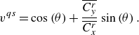 \begin{align} v^{{qs}}=\cos \left (\theta \right )+\dfrac {\overline {C^r_y}}{\overline {C^r_x}}\sin \left (\theta \right ). \end{align}
This estimate of $v$
is identified by the superscript
$v$
is identified by the superscript ${}^{{qs}}$
in reference to the quasi-steady approach. In general, (3.2) is nonlinear as the force coefficients depend on the Reynolds number and rotation rate scaled by the velocity magnitude of the flow seen by the body, and thus on the drift velocity. When the rotation is stopped, the time-averaged transverse force vanishes (
${}^{{qs}}$
in reference to the quasi-steady approach. In general, (3.2) is nonlinear as the force coefficients depend on the Reynolds number and rotation rate scaled by the velocity magnitude of the flow seen by the body, and thus on the drift velocity. When the rotation is stopped, the time-averaged transverse force vanishes ( $\overline {C^r_y}=0$
), which leads to the exact expression of the drift velocity (3.1), derived without quasi-steady assumption. In the absence of fluctuation of the forces, when flow unsteadiness around the drifting body ceases, the quasi-steady approach provides the exact value of the tangential force and, therefore, the exact value of
$\overline {C^r_y}=0$
), which leads to the exact expression of the drift velocity (3.1), derived without quasi-steady assumption. In the absence of fluctuation of the forces, when flow unsteadiness around the drifting body ceases, the quasi-steady approach provides the exact value of the tangential force and, therefore, the exact value of $v$
. The coincidence of
$v$
. The coincidence of $v^{{qs}}$
and
$v^{{qs}}$
and $v$
in steady flow is visualised in figure 3(b-i).
$v$
in steady flow is visualised in figure 3(b-i).
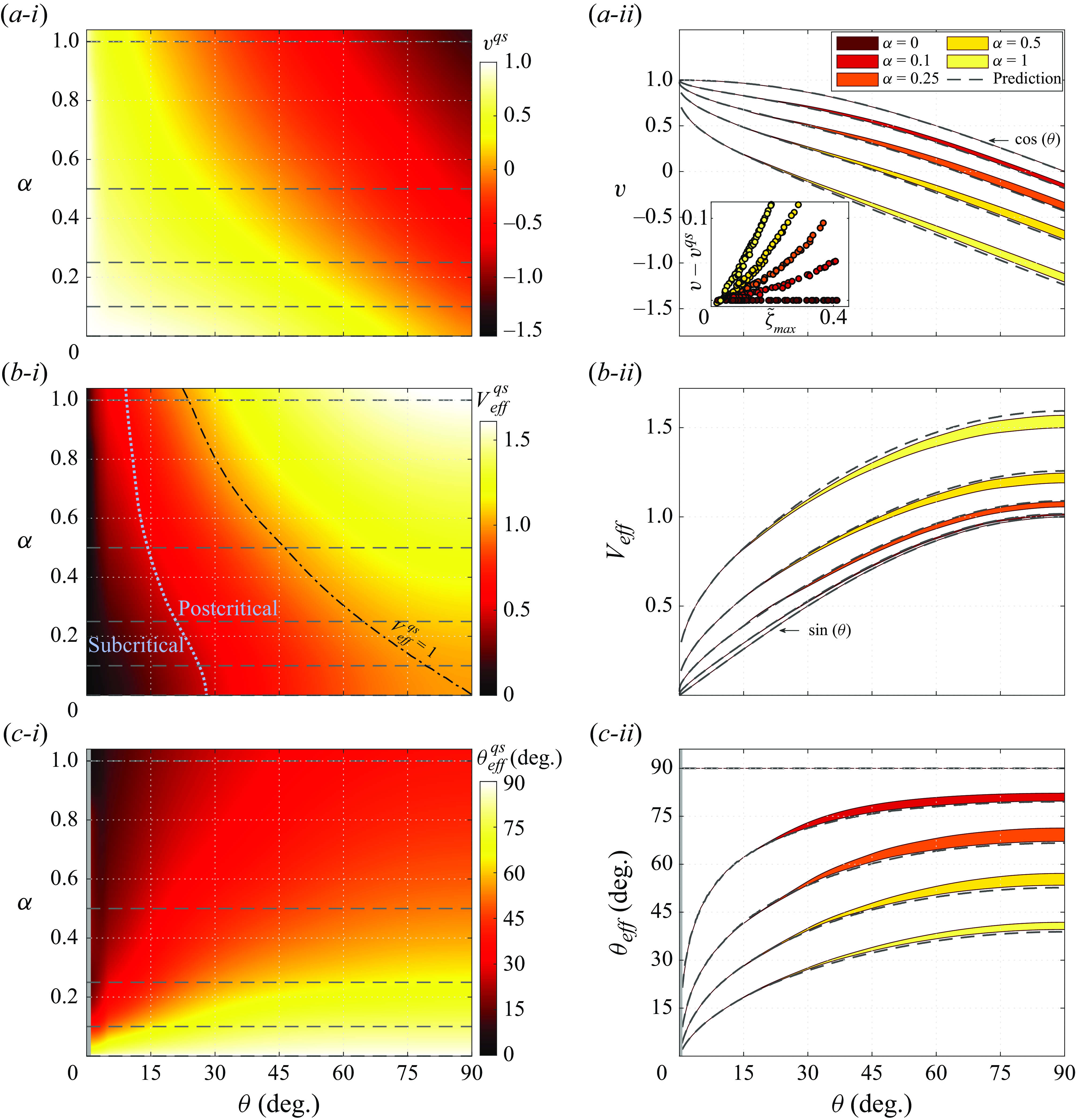
Figure 4. (a) Drift velocity, (b) effective flow velocity magnitude and (c) effective incidence angle, as functions of the incidence angle and rotation rate: (i) maps of the values predicted via the quasi-steady approach and (ii) values issued from the simulations for selected rotation rates. Grey dashed lines indicate the selected rotation rates in (i) and the corresponding predictions in (ii). The expressions of the drift velocity and effective flow velocity magnitude derived by symmetry considerations for $\alpha =0$
are specified in (a-ii) and (b-ii). In (ii), the coloured areas encompass the simulation results obtained for
$\alpha =0$
are specified in (a-ii) and (b-ii). In (ii), the coloured areas encompass the simulation results obtained for $m^\star \in [0.01,1]$
. The inset in (a-ii) depicts the difference between the simulated drift velocity and the predicted value, as a function of the oscillation amplitude, for each rotation rate. In the large-amplitude oscillation cases encountered for
$m^\star \in [0.01,1]$
. The inset in (a-ii) depicts the difference between the simulated drift velocity and the predicted value, as a function of the oscillation amplitude, for each rotation rate. In the large-amplitude oscillation cases encountered for $\theta \approx 0^\circ$
, the simulated and predicted values of
$\theta \approx 0^\circ$
, the simulated and predicted values of $v$
coincide (not visualised in the inset). In (b-i), the iso-contour
$v$
coincide (not visualised in the inset). In (b-i), the iso-contour $V^{{qs}}_{{eff}}=1$
is represented by a black dash-dotted line; the subcritical and postcritical regions are delimited by a light blue dotted line.
$V^{{qs}}_{{eff}}=1$
is represented by a black dash-dotted line; the subcritical and postcritical regions are delimited by a light blue dotted line.
The drift velocity predicted via the quasi-steady approach is plotted in the $(\theta ,\alpha )$
domain in figure 4(a-i), and a comparison of the predicted values with those issued from the simulations is proposed in figure 4(a-ii), for selected rotation rates. In the latter plot, the coloured areas encompass the simulation results obtained for
$(\theta ,\alpha )$
domain in figure 4(a-i), and a comparison of the predicted values with those issued from the simulations is proposed in figure 4(a-ii), for selected rotation rates. In the latter plot, the coloured areas encompass the simulation results obtained for $m^\star \in [0.01,1]$
, while the predicted values are denoted by grey dashed lines. As previously mentioned, the parameter space is covered by two-dimensional simulations. The three-dimensional transition of the flow, when it occurs, has only a limited impact on the structural dynamics, especially on the drift, as illustrated by the three-dimensional simulation results represented for a typical case in figure 3(iii) (green dotted lines). The vision provided by the two-dimensional simulation results appears to be sufficiently accurate to describe the system behaviour. The three-dimensional transition is more specifically addressed in § 3.3.1. It is recalled that the presentation focuses on
$m^\star \in [0.01,1]$
, while the predicted values are denoted by grey dashed lines. As previously mentioned, the parameter space is covered by two-dimensional simulations. The three-dimensional transition of the flow, when it occurs, has only a limited impact on the structural dynamics, especially on the drift, as illustrated by the three-dimensional simulation results represented for a typical case in figure 3(iii) (green dotted lines). The vision provided by the two-dimensional simulation results appears to be sufficiently accurate to describe the system behaviour. The three-dimensional transition is more specifically addressed in § 3.3.1. It is recalled that the presentation focuses on $\theta \in [0^\circ ,90^\circ ]$
since the dynamics over the rest of the
$\theta \in [0^\circ ,90^\circ ]$
since the dynamics over the rest of the $\theta$
range can be directly deduced from these results (Appendix). In particular, if
$\theta$
range can be directly deduced from these results (Appendix). In particular, if $v$
is the drift velocity at incidence
$v$
is the drift velocity at incidence $\theta$
, then the drift velocity at incidence
$\theta$
, then the drift velocity at incidence $180^\circ -\theta$
is equal to
$180^\circ -\theta$
is equal to $v-2\cos (\theta )$
.
$v-2\cos (\theta )$
.
As expected, the predicted values of the drift velocity match the simulation results in the absence of rotation. When the body rotates, the slight deviation between the predicted and simulated values betrays the unsteady nature of the flow and the presence of body oscillation; these aspects are examined later in the paper. Two typical cases where such a deviation is observed are depicted in figure 3(b-ii,b-iii). The inset in figure 4(a-ii) shows that, except for very low incidence angles which are not considered in this plot, the deviation, quantified via the difference $v-v^{{qs}}$
, tends to increase with the oscillation amplitude for each
$v-v^{{qs}}$
, tends to increase with the oscillation amplitude for each $\alpha \gt 0$
. Unless stated otherwise, the oscillation amplitude is measured as the maximum value of the displacement fluctuation about its linear (drift) component. A distinct trend arises at very low incidence, where the prediction is accurate despite the possible emergence of a pronounced unsteadiness of the flow associated with a large oscillation of the cylinder. This is illustrated in figure 3(b-iv) for
$\alpha \gt 0$
. Unless stated otherwise, the oscillation amplitude is measured as the maximum value of the displacement fluctuation about its linear (drift) component. A distinct trend arises at very low incidence, where the prediction is accurate despite the possible emergence of a pronounced unsteadiness of the flow associated with a large oscillation of the cylinder. This is illustrated in figure 3(b-iv) for $\theta =0^\circ$
(
$\theta =0^\circ$
( $v^{{qs}}=v=1$
).
$v^{{qs}}=v=1$
).
At given $\theta$
and
$\theta$
and $\alpha$
, the dispersion of
$\alpha$
, the dispersion of $v$
when the mass ratio and oscillation amplitude vary, i.e. the thickness of the coloured areas in figure 4(a-ii), remains small, and so does the deviation between
$v$
when the mass ratio and oscillation amplitude vary, i.e. the thickness of the coloured areas in figure 4(a-ii), remains small, and so does the deviation between $v$
and
$v$
and $v^{{qs}}$
. This highlights the minor influence of body oscillation and of its modulation by
$v^{{qs}}$
. This highlights the minor influence of body oscillation and of its modulation by $m^\star$
, which are not taken into account in the quasi-steady approach, on the drift velocity. The quasi-steady prediction results can be employed to obtain a global, continuous monitoring of the evolution of the drift velocity, and other related quantities discussed hereafter, across the parameter space.
$m^\star$
, which are not taken into account in the quasi-steady approach, on the drift velocity. The quasi-steady prediction results can be employed to obtain a global, continuous monitoring of the evolution of the drift velocity, and other related quantities discussed hereafter, across the parameter space.
For $\theta =0^\circ$
, the body drifts at the oncoming flow velocity (
$\theta =0^\circ$
, the body drifts at the oncoming flow velocity ( $v=1$
). The drift velocity decreases as the incidence angle is increased. This decreasing trend is enhanced by the forced rotation. The drift velocity, which remains positive for
$v=1$
). The drift velocity decreases as the incidence angle is increased. This decreasing trend is enhanced by the forced rotation. The drift velocity, which remains positive for $\alpha =0$
, may become negative for
$\alpha =0$
, may become negative for $\alpha \gt 0$
. This means that the rotating cylinder may drift upstream, contrary to the non-rotating body. Under forced rotation, the drift velocity reaches high magnitudes, which may exceed the magnitude of the oncoming flow velocity. The conditions associated with the flow seen by the drifting body, and their departure from the nominal conditions based on the oncoming flow, are examined in the following.
$\alpha \gt 0$
. This means that the rotating cylinder may drift upstream, contrary to the non-rotating body. Under forced rotation, the drift velocity reaches high magnitudes, which may exceed the magnitude of the oncoming flow velocity. The conditions associated with the flow seen by the drifting body, and their departure from the nominal conditions based on the oncoming flow, are examined in the following.
3.1.2. Nominal versus effective conditions
The relative flow seen by the body translating at the drift velocity $v$
is called ‘effective flow’. Its velocity in the
$v$
is called ‘effective flow’. Its velocity in the $(x,y,z)$
frame is equal to
$(x,y,z)$
frame is equal to $\{1-v\cos (\theta ),-v\sin (\theta ),0\}^T$
. The effective flow can be schematised as the instantaneous flow in figure 17 (Appendix) by replacing
$\{1-v\cos (\theta ),-v\sin (\theta ),0\}^T$
. The effective flow can be schematised as the instantaneous flow in figure 17 (Appendix) by replacing $\dot \zeta$
by
$\dot \zeta$
by $v$
. The effective flow velocity magnitude and the incidence angle of the rectilinear path with respect to the effective flow, referred to as ‘effective incidence angle’, can be expressed as
$v$
. The effective flow velocity magnitude and the incidence angle of the rectilinear path with respect to the effective flow, referred to as ‘effective incidence angle’, can be expressed as
 \begin{align} V_{{eff}}=\sqrt {v^2-2 v \cos \left (\theta \right )+1}\quad\textrm { and}\quad \theta _{{eff}}=\arctan \left (\dfrac {\sin \left (\theta \right )}{\cos \left (\theta \right )-v}\right ). \end{align}
The effective Reynolds number and rotation rate are defined as
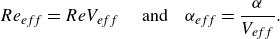 \begin{align} { Re}_{{eff}}={ Re} V_{{eff}}\quad\textrm { and}\quad \alpha _{{eff}}=\dfrac {\alpha }{V_{{eff}}}. \end{align}
These quantities are used to define the actual conditions experienced by the drifting body, named ‘effective conditions’ ( $\theta _{{eff}}$
,
$\theta _{{eff}}$
, ${ Re}_{{eff}}$
,
${ Re}_{{eff}}$
, $\alpha _{{eff}}$
), as opposed to the nominal conditions (
$\alpha _{{eff}}$
), as opposed to the nominal conditions ( $\theta$
,
$\theta$
, ${ Re}$
,
${ Re}$
, $\alpha$
).
$\alpha$
).
For $\alpha =0$
, the expression of the drift velocity (3.1) leads to
$\alpha =0$
, the expression of the drift velocity (3.1) leads to $V_{{eff}}=\sin (\theta )$
and
$V_{{eff}}=\sin (\theta )$
and $\theta _{{eff}}=90^\circ$
. The effective flow velocity magnitude and effective incidence angle based on the quasi-steady prediction of the drift velocity, i.e. (3.3) where
$\theta _{{eff}}=90^\circ$
. The effective flow velocity magnitude and effective incidence angle based on the quasi-steady prediction of the drift velocity, i.e. (3.3) where $v$
is replaced by
$v$
is replaced by $v^{{qs}}$
, can be written in terms of the time-averaged force coefficients:
$v^{{qs}}$
, can be written in terms of the time-averaged force coefficients:
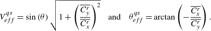 \begin{align} V^{{qs}}_{{eff}}=\sin \left (\theta \right )\sqrt {1+\left (\dfrac {\overline {C^r_y}}{\overline {C^r_x}}\right )^2} \,\,\,\textrm { and}\quad \theta ^{{qs}}_{{eff}}=\arctan \left (-\dfrac {\overline {C^r_x}}{\overline {C^r_y}}\right ). \end{align}
The implicit nature of these expressions, where $\overline {C^r_x}$
and
$\overline {C^r_x}$
and $\overline {C^r_y}$
depend on the Reynolds number and rotation rate scaled by the velocity magnitude of the effective flow, i.e.
$\overline {C^r_y}$
depend on the Reynolds number and rotation rate scaled by the velocity magnitude of the effective flow, i.e. ${ Re}_{{eff}}$
and
${ Re}_{{eff}}$
and $\alpha _{{eff}}$
or their quasi-steady estimates in the present case, may render the quantification of rotation effects hazardous. Some trends can however be conjectured. The above expression of
$\alpha _{{eff}}$
or their quasi-steady estimates in the present case, may render the quantification of rotation effects hazardous. Some trends can however be conjectured. The above expression of $V^{{qs}}_{{eff}}$
predicts a systematic amplification of the effective flow velocity magnitude by the rotation, regardless of
$V^{{qs}}_{{eff}}$
predicts a systematic amplification of the effective flow velocity magnitude by the rotation, regardless of $\alpha$
, due to the emergence of a time-averaged transverse force (
$\alpha$
, due to the emergence of a time-averaged transverse force ( $\overline {C^r_y}\ne 0$
). As long as
$\overline {C^r_y}\ne 0$
). As long as $\overline {C^r_x}\gt 0$
and
$\overline {C^r_x}\gt 0$
and $\overline {C^r_y}\lt 0$
, which is expected to occur over a wide portion of the parameter space, the effective incidence angle should be positive but lower than
$\overline {C^r_y}\lt 0$
, which is expected to occur over a wide portion of the parameter space, the effective incidence angle should be positive but lower than $90^\circ$
. For
$90^\circ$
. For ${ Re}_r=100$
and
${ Re}_r=100$
and $\alpha _r\in [0,1]$
, the magnitude of the ratio
$\alpha _r\in [0,1]$
, the magnitude of the ratio $\overline {C^r_y}/\overline {C^r_x}$
increases with
$\overline {C^r_y}/\overline {C^r_x}$
increases with $\alpha _r$
. Therefore, the incidence angle where the drift ceases and where the nominal and effective conditions coincide (
$\alpha _r$
. Therefore, the incidence angle where the drift ceases and where the nominal and effective conditions coincide ( $V_{{eff}}=1$
and
$V_{{eff}}=1$
and $\theta _{{eff}}=\theta$
) should move from
$\theta _{{eff}}=\theta$
) should move from $\theta =90^\circ$
for
$\theta =90^\circ$
for $\alpha =0$
, towards lower values, as
$\alpha =0$
, towards lower values, as $\alpha$
is increased. This trend can equally be inferred via (3.2).
$\alpha$
is increased. This trend can equally be inferred via (3.2).
The values of $V^{{qs}}_{{eff}}$
and
$V^{{qs}}_{{eff}}$
and $\theta ^{{qs}}_{{eff}}$
are represented in the
$\theta ^{{qs}}_{{eff}}$
are represented in the $(\theta ,\alpha )$
domain in figure 4(b-i,c-i), and compared with the simulation results in figure 4(b-ii,c-ii). The evolutions of the effective flow velocity magnitude and effective incidence angle with
$(\theta ,\alpha )$
domain in figure 4(b-i,c-i), and compared with the simulation results in figure 4(b-ii,c-ii). The evolutions of the effective flow velocity magnitude and effective incidence angle with $\theta$
are symmetrical about
$\theta$
are symmetrical about $\theta = 90^\circ$
. As previously noted for the drift velocity,
$\theta = 90^\circ$
. As previously noted for the drift velocity, $V_{{eff}}$
and
$V_{{eff}}$
and $\theta _{{eff}}$
exhibit small dispersions as
$\theta _{{eff}}$
exhibit small dispersions as $m^\star$
is varied, and their trends are globally well predicted by the quasi-steady approach. These plots illustrate the marginal influence of body oscillation on the effective conditions.
$m^\star$
is varied, and their trends are globally well predicted by the quasi-steady approach. These plots illustrate the marginal influence of body oscillation on the effective conditions.
Independently of the rotation rate, the body sees no effective flow when the direction of motion is aligned with the oncoming flow ( $V_{{eff}}=0$
). The magnitude of the effective flow velocity increases with
$V_{{eff}}=0$
). The magnitude of the effective flow velocity increases with $\theta$
and reaches its peak value at normal incidence. As conjectured above,
$\theta$
and reaches its peak value at normal incidence. As conjectured above, $V_{{eff}}$
is amplified by the forced rotation. It may become substantially larger than
$V_{{eff}}$
is amplified by the forced rotation. It may become substantially larger than $1$
, which corresponds to the maximum value attained for
$1$
, which corresponds to the maximum value attained for $\alpha =0$
, and to the oncoming flow velocity magnitude. To visualise this effect, the iso-contour
$\alpha =0$
, and to the oncoming flow velocity magnitude. To visualise this effect, the iso-contour $V^{{qs}}_{{eff}}=1$
is superimposed on the map of figure 4(b-i). This iso-contour delineates the cases where the effective conditions match the nominal conditions, which tend to occur at lower
$V^{{qs}}_{{eff}}=1$
is superimposed on the map of figure 4(b-i). This iso-contour delineates the cases where the effective conditions match the nominal conditions, which tend to occur at lower $\theta$
when
$\theta$
when $\alpha$
is increased, as suggested by (3.5).
$\alpha$
is increased, as suggested by (3.5).
For $\alpha =0$
, the effective incidence angle remains equal to
$\alpha =0$
, the effective incidence angle remains equal to $90^\circ$
regardless of
$90^\circ$
regardless of $\theta$
. As a result, the configuration seen by the non-rotating body presents a transverse symmetry relative to the effective flow, despite the asymmetry of the nominal configuration (for
$\theta$
. As a result, the configuration seen by the non-rotating body presents a transverse symmetry relative to the effective flow, despite the asymmetry of the nominal configuration (for $\theta \ne 90^\circ$
). This phenomenon of symmetry recovery, due to the drift, does not exist for an elastically mounted body. It is closely connected to the symmetry properties of the structural oscillation and wake organisation, as discussed in §§ 3.2.1 and 3.3.1. In contrast, the effective incidence angle varies with
$\theta \ne 90^\circ$
). This phenomenon of symmetry recovery, due to the drift, does not exist for an elastically mounted body. It is closely connected to the symmetry properties of the structural oscillation and wake organisation, as discussed in §§ 3.2.1 and 3.3.1. In contrast, the effective incidence angle varies with $\theta$
once the body rotates. It remains positive and lower than
$\theta$
once the body rotates. It remains positive and lower than $90^\circ$
, as expected, with an increasing trend versus
$90^\circ$
, as expected, with an increasing trend versus $\theta$
and a decreasing trend as
$\theta$
and a decreasing trend as $\alpha$
is increased. It appears that the imposed rotation restrains the effective incidence to low angles, which do not exceed
$\alpha$
is increased. It appears that the imposed rotation restrains the effective incidence to low angles, which do not exceed $45^\circ$
for
$45^\circ$
for $\alpha =1$
.
$\alpha =1$
.
A complementary vision of the parameter space explored when the cylinder drifts is proposed in figure 5, where the effective Reynolds number and rotation rate are plotted as functions of the effective incidence angle. For each $\alpha$
, the coloured areas regroup the simulation results obtained for
$\alpha$
, the coloured areas regroup the simulation results obtained for $m^\star \in [0.01,1]$
as
$m^\star \in [0.01,1]$
as $\theta$
is varied, and the values predicted via the quasi-steady approach, thus independent of
$\theta$
is varied, and the values predicted via the quasi-steady approach, thus independent of $m^\star$
, are represented by grey dashed lines. The effective flow tends to vanish close to
$m^\star$
, are represented by grey dashed lines. The effective flow tends to vanish close to $\theta = 0^\circ$
;
$\theta = 0^\circ$
; $\theta _{{eff}}$
is not defined in this case. The results are plotted down to
$\theta _{{eff}}$
is not defined in this case. The results are plotted down to $\theta \approx 0.5^\circ$
. These plots depict the departure of the effective conditions from the nominal ones. Compared with the fixed nominal Re of
$\theta \approx 0.5^\circ$
. These plots depict the departure of the effective conditions from the nominal ones. Compared with the fixed nominal Re of $100$
, the drifting body may be exposed to a wide range of effective Reynolds numbers, up to
$100$
, the drifting body may be exposed to a wide range of effective Reynolds numbers, up to $160$
approximately for
$160$
approximately for $\alpha =1$
. The
$\alpha =1$
. The $({ Re}_{{eff}},\alpha _{{eff}})$
domain visited by the system includes the critical boundary that delimits the onset of flow unsteadiness for a rigidly mounted cylinder. This boundary is indicated by blue dotted segments in figure 5(a). A slight deviation between the quasi-steady prediction of
$({ Re}_{{eff}},\alpha _{{eff}})$
domain visited by the system includes the critical boundary that delimits the onset of flow unsteadiness for a rigidly mounted cylinder. This boundary is indicated by blue dotted segments in figure 5(a). A slight deviation between the quasi-steady prediction of ${ Re}_{{eff}}$
and its actual values can be observed below this boundary. It reflects the existence of flow unsteadiness and body oscillation in the subcritical region, as previously reported at normal incidence without rotation (Ryan et al. Reference Ryan, Thompson and Hourigan2005; Bourguet Reference Bourguet2023a
); this point is studied in § 3.2.1. The critical boundary is plotted in the
${ Re}_{{eff}}$
and its actual values can be observed below this boundary. It reflects the existence of flow unsteadiness and body oscillation in the subcritical region, as previously reported at normal incidence without rotation (Ryan et al. Reference Ryan, Thompson and Hourigan2005; Bourguet Reference Bourguet2023a
); this point is studied in § 3.2.1. The critical boundary is plotted in the $(\theta ,\alpha )$
domain in figure 4(b-i) (blue dotted line). The location of the critical boundary shifts from
$(\theta ,\alpha )$
domain in figure 4(b-i) (blue dotted line). The location of the critical boundary shifts from $\theta \approx 28^\circ$
to
$\theta \approx 28^\circ$
to $\theta \approx 10^\circ$
as
$\theta \approx 10^\circ$
as $\alpha$
is increased from
$\alpha$
is increased from $0$
to
$0$
to $1$
. The
$1$
. The $({ Re}_{{eff}},\alpha _{{eff}})$
domain explored by the system does not include the threshold of the three-dimensional transition in the flow past a rigidly mounted cylinder, examined for example by Rao et al. (Reference Rao, Radi, Leontini, Thompson, Sheridan and Hourigan2015). Yet, this does not prevent the present flow from becoming three-dimensional under the effect of body oscillation, as shown in § 3.3.1.
$({ Re}_{{eff}},\alpha _{{eff}})$
domain explored by the system does not include the threshold of the three-dimensional transition in the flow past a rigidly mounted cylinder, examined for example by Rao et al. (Reference Rao, Radi, Leontini, Thompson, Sheridan and Hourigan2015). Yet, this does not prevent the present flow from becoming three-dimensional under the effect of body oscillation, as shown in § 3.3.1.
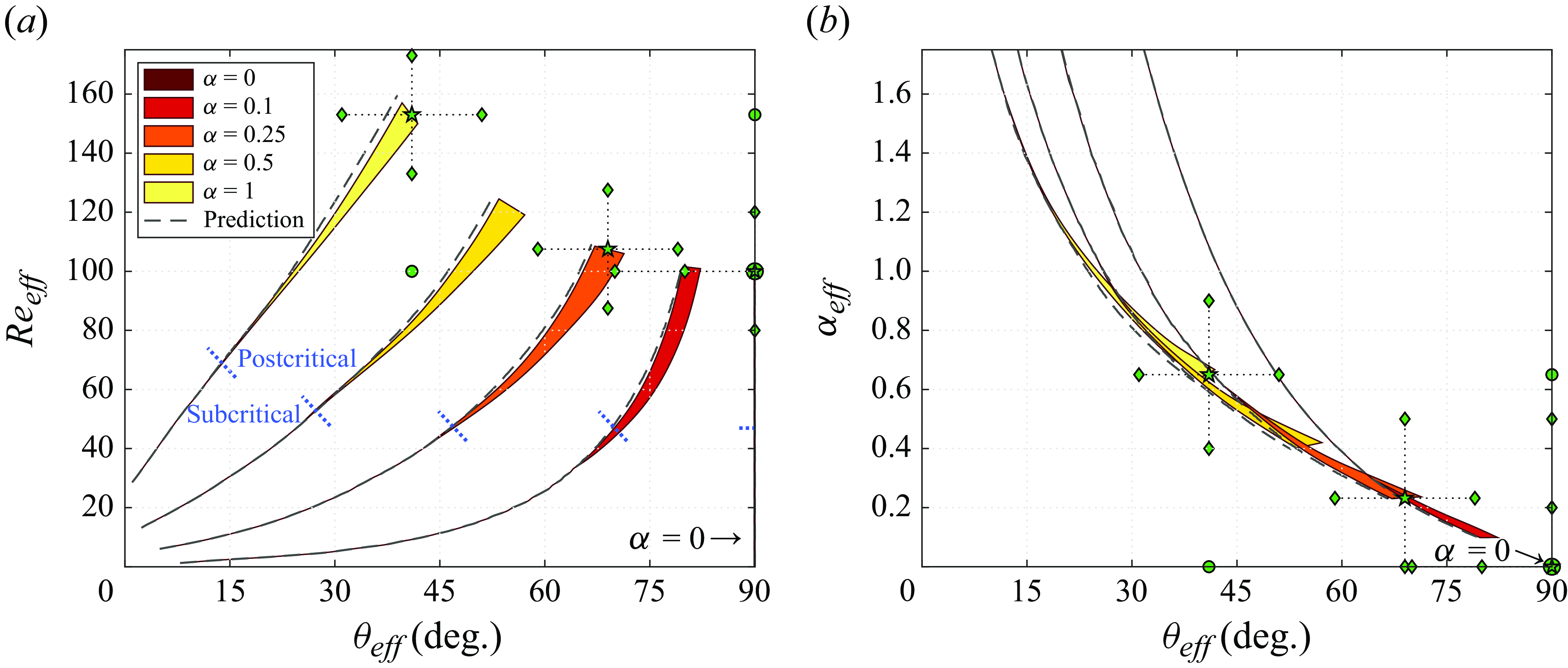
Figure 5. Effective (a) Reynolds number and (b) rotation rate as functions of the effective incidence angle, for selected rotation rates. The coloured areas encompass the values measured in the $(\theta ,m^\star )$
domain for each rotation rate (simulation results). The quasi-steady prediction results are represented by grey dashed lines. The results are plotted down to
$(\theta ,m^\star )$
domain for each rotation rate (simulation results). The quasi-steady prediction results are represented by grey dashed lines. The results are plotted down to $\theta \approx 0.5^\circ$
. In (a), the subcritical and postcritical regions are delimited by blue dotted segments. Green symbols denote the cases with SRF examined in figures 14 (stars), 15 (dots) and 16 (diamonds).
$\theta \approx 0.5^\circ$
. In (a), the subcritical and postcritical regions are delimited by blue dotted segments. Green symbols denote the cases with SRF examined in figures 14 (stars), 15 (dots) and 16 (diamonds).
The above observations can be summarised as follows. The drift, which is only marginally affected by body oscillation/flow unsteadiness and variations of $m^\star$
, can be predicted via a quasi-steady modelling of fluid forcing. The effective conditions, associated with the flow seen by the drifting body, may considerably differ from the nominal ones. Contrary to the nominal conditions, the effective conditions include the critical threshold of flow unsteadiness for a rigidly mounted cylinder, and the effective flow may even vanish when body trajectory is aligned with the oncoming flow. The imposed rotation causes an amplification of the effective flow. This results in a substantial increase of the maximum value of the effective Reynolds number. The transverse symmetry of the system relative to the effective flow, which persists in asymmetrical nominal configurations for a non-rotating cylinder, is broken once the body rotates. The rotation introduces a dependence of the effective incidence on
$m^\star$
, can be predicted via a quasi-steady modelling of fluid forcing. The effective conditions, associated with the flow seen by the drifting body, may considerably differ from the nominal ones. Contrary to the nominal conditions, the effective conditions include the critical threshold of flow unsteadiness for a rigidly mounted cylinder, and the effective flow may even vanish when body trajectory is aligned with the oncoming flow. The imposed rotation causes an amplification of the effective flow. This results in a substantial increase of the maximum value of the effective Reynolds number. The transverse symmetry of the system relative to the effective flow, which persists in asymmetrical nominal configurations for a non-rotating cylinder, is broken once the body rotates. The rotation introduces a dependence of the effective incidence on $\theta$
, and tends to restrain it to low angles. The possible oscillation of the cylinder about its drifting motion and the interaction regimes will be investigated in relation to these effective conditions.
$\theta$
, and tends to restrain it to low angles. The possible oscillation of the cylinder about its drifting motion and the interaction regimes will be investigated in relation to these effective conditions.
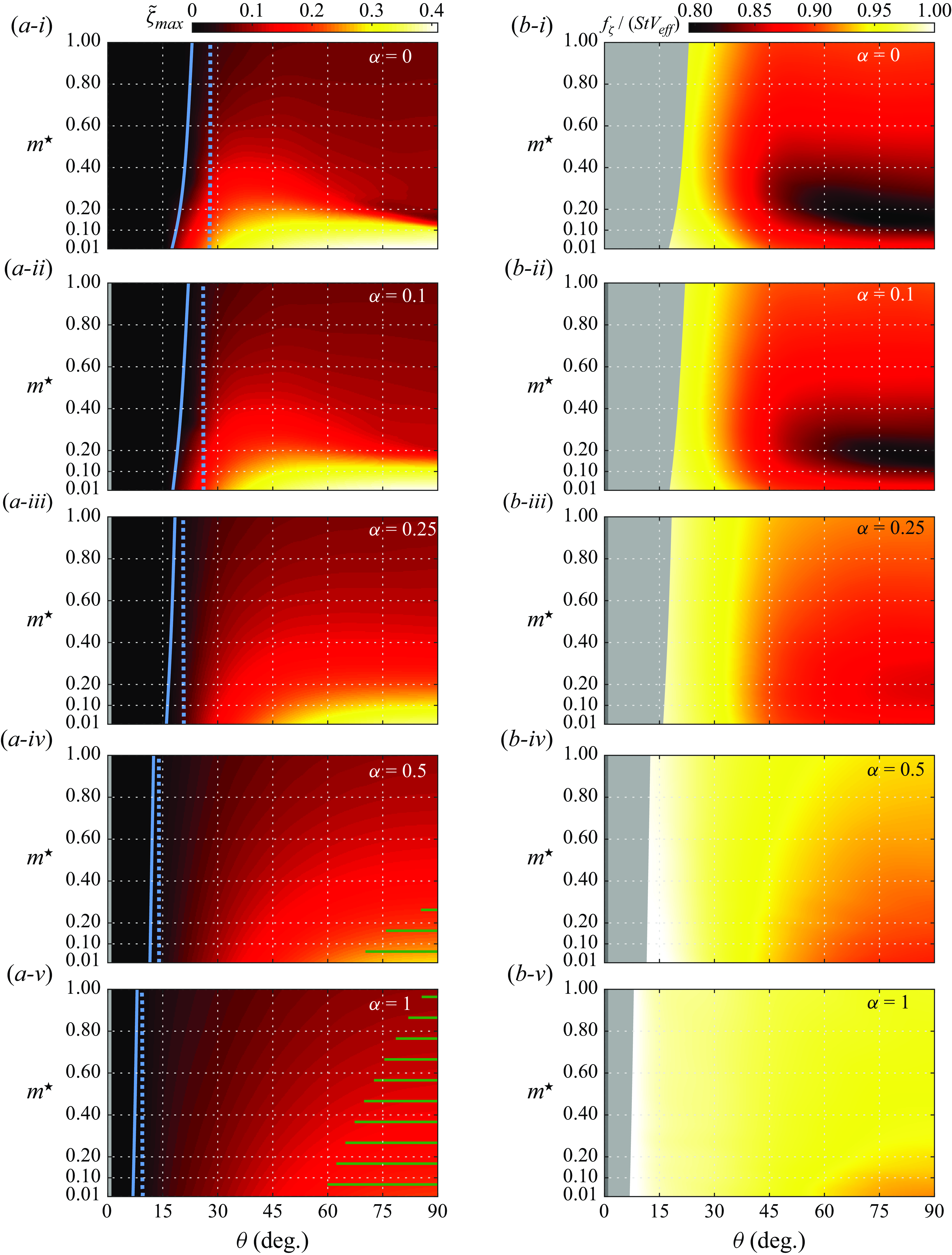
Figure 6. Oscillation (a) amplitude and (b) frequency as functions of the incidence angle and mass ratio, for (i) $\alpha =0$
, (ii)
$\alpha =0$
, (ii) $\alpha =0.1$
, (iii)
$\alpha =0.1$
, (iii) $\alpha =0.25$
, (iv)
$\alpha =0.25$
, (iv) $\alpha =0.5$
and (v)
$\alpha =0.5$
and (v) $\alpha =1$
. The oscillation frequency is normalised by the effective flow velocity magnitude (
$\alpha =1$
. The oscillation frequency is normalised by the effective flow velocity magnitude ( $V_{{eff}}$
) and the Strouhal frequency measured at the effective Reynolds number and rotation rate (
$V_{{eff}}$
) and the Strouhal frequency measured at the effective Reynolds number and rotation rate ( ${ Re}_{{eff}}$
and
${ Re}_{{eff}}$
and $\alpha _{{eff}}$
). In (a), the subcritical and postcritical regions are delimited by a blue dotted line, while a blue solid line delineates the oscillation (VIV) region. In (ii)–(v), the region close to
$\alpha _{{eff}}$
). In (a), the subcritical and postcritical regions are delimited by a blue dotted line, while a blue solid line delineates the oscillation (VIV) region. In (ii)–(v), the region close to $\theta =0^\circ$
is masked; it is specifically examined in § 3.2.2. The horizontal stripes in (a-iv) and (a-v) indicate the area where the flow is three-dimensional.
$\theta =0^\circ$
is masked; it is specifically examined in § 3.2.2. The horizontal stripes in (a-iv) and (a-v) indicate the area where the flow is three-dimensional.
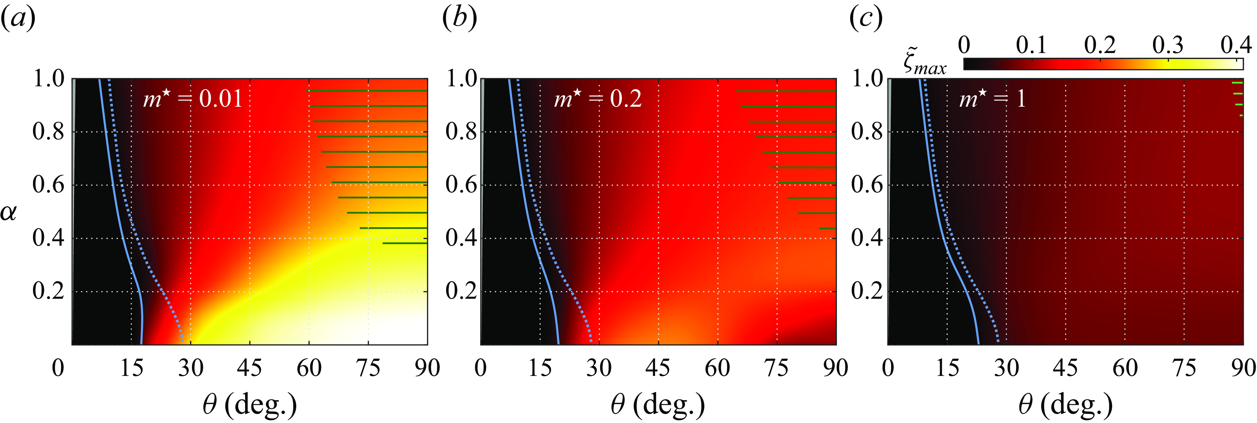
Figure 7. Oscillation amplitude as a function of the incidence angle and rotation rate, for (a) $m^\star =0.01$
, (b)
$m^\star =0.01$
, (b) $m^\star =0.2$
and (c)
$m^\star =0.2$
and (c) $m^\star =1$
. The subcritical and postcritical regions are delimited by a blue dotted line. A blue solid line delineates the oscillation (VIV) region. The region close to
$m^\star =1$
. The subcritical and postcritical regions are delimited by a blue dotted line. A blue solid line delineates the oscillation (VIV) region. The region close to $\theta =0^\circ$
is masked; it is examined in § 3.2.2. The horizontal stripes indicate the area where the flow is three-dimensional.
$\theta =0^\circ$
is masked; it is examined in § 3.2.2. The horizontal stripes indicate the area where the flow is three-dimensional.
3.2. Oscillation of the drifting body
An oscillation of the cylinder may spontaneously develop about the linear component of its displacement, as shown in figure 3. Prior works have documented the emergence of transverse VIV for a non-rotating cylinder without SRF, including at the present Reynolds number of $100$
(Shiels et al. Reference Shiels, Leonard and Roshko2001; Navrose & Mittal Reference Mittal2017; Bourguet Reference Bourguet2023a
). The persistence of this form of structural response, as the rectilinear path is inclined and the body subjected to a forced rotation, is studied in § 3.2.1. A second form of oscillation, appearing close to
$100$
(Shiels et al. Reference Shiels, Leonard and Roshko2001; Navrose & Mittal Reference Mittal2017; Bourguet Reference Bourguet2023a
). The persistence of this form of structural response, as the rectilinear path is inclined and the body subjected to a forced rotation, is studied in § 3.2.1. A second form of oscillation, appearing close to $\theta = 0^\circ$
, is examined in § 3.2.2.
$\theta = 0^\circ$
, is examined in § 3.2.2.
3.2.1. Vortex-induced vibrations
The $(\theta ,\alpha )$
domain investigated represents an extension of the canonical configuration addressed in previous studies concerning VIV without SRF, i.e.
$(\theta ,\alpha )$
domain investigated represents an extension of the canonical configuration addressed in previous studies concerning VIV without SRF, i.e. $\theta = 90^\circ$
and
$\theta = 90^\circ$
and $\alpha = 0$
. The body oscillation amplitude and frequency are plotted in the
$\alpha = 0$
. The body oscillation amplitude and frequency are plotted in the $(\theta ,m^\star )$
domain in figure 6, for selected rotation rates, and a complementary visualisation of the oscillation amplitude in the
$(\theta ,m^\star )$
domain in figure 6, for selected rotation rates, and a complementary visualisation of the oscillation amplitude in the $(\theta ,\alpha )$
domain is proposed in figure 7, for selected mass ratios. The evolutions of the oscillation amplitude and frequency with
$(\theta ,\alpha )$
domain is proposed in figure 7, for selected mass ratios. The evolutions of the oscillation amplitude and frequency with $\theta$
are symmetrical about
$\theta$
are symmetrical about $\theta = 90^\circ$
, since the displacement fluctuation is the same at incidences
$\theta = 90^\circ$
, since the displacement fluctuation is the same at incidences $\theta$
and
$\theta$
and $180^\circ -\theta$
(Appendix). These plots are based on two-dimensional simulation results. The three-dimensional transition of the flow (examined in § 3.3.1) has only a limited impact on the structural dynamics.
$180^\circ -\theta$
(Appendix). These plots are based on two-dimensional simulation results. The three-dimensional transition of the flow (examined in § 3.3.1) has only a limited impact on the structural dynamics.
Starting from the normal incidence configuration ( $\theta =90^\circ$
), body oscillation is found to occur down to an incidence angle that increases with
$\theta =90^\circ$
), body oscillation is found to occur down to an incidence angle that increases with $m^\star$
and decreases as
$m^\star$
and decreases as $\alpha$
is increased, from
$\alpha$
is increased, from $\theta \approx 23^\circ$
for
$\theta \approx 23^\circ$
for $(m^\star ,\alpha )=(1,0)$
to
$(m^\star ,\alpha )=(1,0)$
to $\theta \approx 7^\circ$
for
$\theta \approx 7^\circ$
for $(m^\star ,\alpha )=(0.01,1)$
. The region where the cylinder oscillates is delimited by a blue solid line in figures 6(a) and 7. At given
$(m^\star ,\alpha )=(0.01,1)$
. The region where the cylinder oscillates is delimited by a blue solid line in figures 6(a) and 7. At given $m^\star$
and
$m^\star$
and $\alpha$
, the incidence angle, where the critical conditions, in terms of
$\alpha$
, the incidence angle, where the critical conditions, in terms of ${ Re}_{{eff}}$
and
${ Re}_{{eff}}$
and $\alpha _{{eff}}$
, are reached (blue dotted line), is always located within the oscillation region. It is recalled that the critical conditions refer to the onset of flow unsteadiness for a rigidly mounted body. This defines a zone of subcritical response, which tends to shrink as
$\alpha _{{eff}}$
, are reached (blue dotted line), is always located within the oscillation region. It is recalled that the critical conditions refer to the onset of flow unsteadiness for a rigidly mounted body. This defines a zone of subcritical response, which tends to shrink as $m^\star$
and
$m^\star$
and $\alpha$
are increased. When
$\alpha$
are increased. When $\theta$
is reduced below the edge of the oscillation region, the body moves at a constant velocity, the drift velocity
$\theta$
is reduced below the edge of the oscillation region, the body moves at a constant velocity, the drift velocity $v$
, and is exposed to a steady flow. An example of this state of the system is depicted in figure 3(i). A second form of oscillation arises close to
$v$
, and is exposed to a steady flow. An example of this state of the system is depicted in figure 3(i). A second form of oscillation arises close to $\theta = 0^\circ$
. It is specifically analysed in § 3.2.2 and the corresponding region is masked in the plots of figures 6 and 7.
$\theta = 0^\circ$
. It is specifically analysed in § 3.2.2 and the corresponding region is masked in the plots of figures 6 and 7.
Two typical examples of the responses encountered in the oscillation region delineated in figures 6(a) and 7 are visualised in figure 3(ii,iii). Figure 3(iii) also illustrates the marginal influence of the flow three-dimensional transition. In all studied cases, the body displacement fluctuation is periodic and close to sinusoidal. This justifies the choices made to measure the oscillation amplitude and frequency, i.e. maximum value of $\tilde \zeta$
and Fourier transform of its time series, respectively. The oscillation frequency
$\tilde \zeta$
and Fourier transform of its time series, respectively. The oscillation frequency $f_\zeta$
refers to the frequency of the dominant component of
$f_\zeta$
refers to the frequency of the dominant component of $\tilde \zeta$
spectrum, which is also its fundamental component in all cases. The higher harmonics that can arise in this spectrum have a minor contribution, usually lower than
$\tilde \zeta$
spectrum, which is also its fundamental component in all cases. The higher harmonics that can arise in this spectrum have a minor contribution, usually lower than $5\,\%$
of the fundamental component amplitude, but they reflect response symmetry. For
$5\,\%$
of the fundamental component amplitude, but they reflect response symmetry. For $\alpha =0$
, as shown in § 3.1.2, the system exhibits a phenomenon of symmetry recovery and the effective configuration remains symmetrical (
$\alpha =0$
, as shown in § 3.1.2, the system exhibits a phenomenon of symmetry recovery and the effective configuration remains symmetrical ( $\theta _{{eff}}=90^\circ$
) regardless of
$\theta _{{eff}}=90^\circ$
) regardless of $\theta$
. In this case, the displacement fluctuation also exhibits a transverse symmetry and only odd harmonics occur in its spectrum. For
$\theta$
. In this case, the displacement fluctuation also exhibits a transverse symmetry and only odd harmonics occur in its spectrum. For $\alpha \gt 0$
, the transverse symmetry is broken and even harmonics may appear. Their presence is betrayed by slight differences in the magnitudes of the positive and negative extrema of displacement fluctuation.
$\alpha \gt 0$
, the transverse symmetry is broken and even harmonics may appear. Their presence is betrayed by slight differences in the magnitudes of the positive and negative extrema of displacement fluctuation.
The peak amplitude of oscillation, close to $0.4D$
, is attained at normal incidence, without rotation, and for the lowest mass ratio (
$0.4D$
, is attained at normal incidence, without rotation, and for the lowest mass ratio ( $m^\star =0.01$
). For
$m^\star =0.01$
). For $\alpha =0$
, an amplitude larger than
$\alpha =0$
, an amplitude larger than $0.3D$
persists, in the lower-
$0.3D$
persists, in the lower- $m^\star$
range, down to
$m^\star$
range, down to $\theta \approx 35^\circ$
. A pronounced reduction of the oscillation amplitude occurs as
$\theta \approx 35^\circ$
. A pronounced reduction of the oscillation amplitude occurs as $m^\star$
is increased above
$m^\star$
is increased above $0.1{-}0.15$
. This amplitude drop was associated with the concept of ‘critical mass ratio’ in prior works (e.g. Govardhan & Williamson Reference Govardhan and Williamson2002). The precise location of the drop along the
$0.1{-}0.15$
. This amplitude drop was associated with the concept of ‘critical mass ratio’ in prior works (e.g. Govardhan & Williamson Reference Govardhan and Williamson2002). The precise location of the drop along the $m^\star$
axis and its sharpness depend on
$m^\star$
axis and its sharpness depend on $\theta$
, but the amplitude measured beyond this drop is relatively uniform, around
$\theta$
, but the amplitude measured beyond this drop is relatively uniform, around $0.1D$
. The variation of
$0.1D$
. The variation of $\theta$
at fixed Re is equivalent to a variation of Re (scaled by
$\theta$
at fixed Re is equivalent to a variation of Re (scaled by $\sin (\theta )$
) at normal incidence. The trends observed here were previously visualised in this case (Navrose & Mittal Reference Mittal2017; Bourguet Reference Bourguet2023a
). In particular, the critical mass ratio tends to increase and the amplitude drop tends to be smoother for lower Re at normal incidence and, therefore, for lower
$\sin (\theta )$
) at normal incidence. The trends observed here were previously visualised in this case (Navrose & Mittal Reference Mittal2017; Bourguet Reference Bourguet2023a
). In particular, the critical mass ratio tends to increase and the amplitude drop tends to be smoother for lower Re at normal incidence and, therefore, for lower $\theta$
in the present problem. In the absence of rotation, the oscillation region extends down to
$\theta$
in the present problem. In the absence of rotation, the oscillation region extends down to $\theta \approx 18^\circ$
, which corresponds to Re
$\theta \approx 18^\circ$
, which corresponds to Re $\approx 30$
at normal incidence and thus confirms the Re threshold reported in Bourguet (Reference Bourguet2023a
).
$\approx 30$
at normal incidence and thus confirms the Re threshold reported in Bourguet (Reference Bourguet2023a
).
Under forced rotation, the largest values of response amplitude are still encountered in the lower- $m^\star$
range, but they are smaller than those measured for
$m^\star$
range, but they are smaller than those measured for $\alpha =0$
. As an example, the peak amplitude reached for
$\alpha =0$
. As an example, the peak amplitude reached for $\alpha =1$
(
$\alpha =1$
( $\theta = 90^\circ$
and
$\theta = 90^\circ$
and $m^\star =0.01$
) is slightly larger than
$m^\star =0.01$
) is slightly larger than $0.2D$
, i.e. half of the peak amplitude for
$0.2D$
, i.e. half of the peak amplitude for $\alpha =0$
. To facilitate the comparison, the colour levels are kept the same in the plots of figures 6 and 7. Once the cylinder rotates, the amplitude diminishes more regularly as
$\alpha =0$
. To facilitate the comparison, the colour levels are kept the same in the plots of figures 6 and 7. Once the cylinder rotates, the amplitude diminishes more regularly as $\theta$
is decreased from
$\theta$
is decreased from $90^\circ$
: the plateau identified down to
$90^\circ$
: the plateau identified down to $\theta \approx 35^\circ$
for
$\theta \approx 35^\circ$
for $\alpha =0$
tends to vanish. The amplitude drop observed without rotation along the
$\alpha =0$
tends to vanish. The amplitude drop observed without rotation along the $m^\star$
axis is considerably attenuated. In the higher-
$m^\star$
axis is considerably attenuated. In the higher- $m^\star$
range, the amplitude is globally unaltered by the rotation and remains close to
$m^\star$
range, the amplitude is globally unaltered by the rotation and remains close to $0.1D$
. Overall, the rotation is found to reduce the oscillation amplitude in the lower-
$0.1D$
. Overall, the rotation is found to reduce the oscillation amplitude in the lower- $m^\star$
range, homogenise it and smooth its evolution in the
$m^\star$
range, homogenise it and smooth its evolution in the $(\theta ,m^\star )$
domain.
$(\theta ,m^\star )$
domain.
To quantify the deviation of the oscillation frequency from the frequency of flow unsteadiness in the rigidly mounted body case, in figure 6(b), $f_\zeta$
is normalised by the velocity magnitude of the effective flow seen by the cylinder (
$f_\zeta$
is normalised by the velocity magnitude of the effective flow seen by the cylinder ( $V_{{eff}}$
), and by the Strouhal frequency (St), determined at the effective Reynolds number and rotation rate (
$V_{{eff}}$
), and by the Strouhal frequency (St), determined at the effective Reynolds number and rotation rate ( ${ Re}_{{eff}}$
and
${ Re}_{{eff}}$
and $\alpha _{{eff}}$
). In the subcritical region of the parameter space, the values of St are those obtained without rotation by Kou et al. (Reference Kou, Zhang, Liu and Li2017), by triggering the flow. The influence of the rotation on St is neglected in the subcritical zone, which appears reasonable considering the small variation of St with the rotation rate for
$\alpha _{{eff}}$
). In the subcritical region of the parameter space, the values of St are those obtained without rotation by Kou et al. (Reference Kou, Zhang, Liu and Li2017), by triggering the flow. The influence of the rotation on St is neglected in the subcritical zone, which appears reasonable considering the small variation of St with the rotation rate for $\alpha _r\lt 2$
(e.g. Kang et al. Reference Kang, Choi and Lee1999; Mittal & Kumar Reference Mittal and Kumar2003); here,
$\alpha _r\lt 2$
(e.g. Kang et al. Reference Kang, Choi and Lee1999; Mittal & Kumar Reference Mittal and Kumar2003); here, $\alpha _{{eff}}\lt 1.7$
. The validity of this assumption is corroborated by the proximity between St and body oscillation/flow unsteadiness frequency in this zone, as shown hereafter.
$\alpha _{{eff}}\lt 1.7$
. The validity of this assumption is corroborated by the proximity between St and body oscillation/flow unsteadiness frequency in this zone, as shown hereafter.
The oscillation frequency remains close to the Strouhal frequency. This suggests a connection between body motion and flow unsteadiness, which is indeed verified since they are synchronised throughout the oscillation region. Flow–body synchronisation and its implications for wake organisation are analysed in § 3.3.1. For $\alpha =0$
, the frequency ratio ranges from
$\alpha =0$
, the frequency ratio ranges from $0.8$
to
$0.8$
to $1$
. As shown in prior works on VIV without SRF (Navrose & Mittal Reference Mittal2017; Bourguet Reference Bourguet2024), the peak of deviation from St is shifted towards higher
$1$
. As shown in prior works on VIV without SRF (Navrose & Mittal Reference Mittal2017; Bourguet Reference Bourguet2024), the peak of deviation from St is shifted towards higher $m^\star$
compared with the peak amplitude, and actually occurs close to the amplitude drop. The frequency ratio is also lower than
$m^\star$
compared with the peak amplitude, and actually occurs close to the amplitude drop. The frequency ratio is also lower than $1$
when the cylinder rotates, but the deviation from St is restrained to narrower ranges; it does not exceed
$1$
when the cylinder rotates, but the deviation from St is restrained to narrower ranges; it does not exceed $-8\,\%$
(frequency ratio equal to
$-8\,\%$
(frequency ratio equal to $0.92$
) for
$0.92$
) for $\alpha =1$
. The homogenisation of the amplitude across the oscillation region is accompanied by a homogenisation of the frequency ratio.
$\alpha =1$
. The homogenisation of the amplitude across the oscillation region is accompanied by a homogenisation of the frequency ratio.
Path inclination and cylinder rotation modulate the VIV observed at normal incidence for $\alpha =0$
. Among other effects, body oscillation vanishes below a certain incidence angle and, within the region where an oscillation appears, the rotation causes a homogenisation of its properties, with a notable attenuation of the peak amplitude responses. This attenuation is explored in § 3.3.3 via an analogy with the behaviour of the system with SRF. Yet, several fundamental features of the VIV occurring in the above canonical configuration, some of which also commonly reported for VIV with SRF in this Reynolds number range, persist throughout the oscillation region. These features include the regularity of the oscillation (i.e. its nearly sinusoidal nature), the connection with flow unsteadiness, the order of magnitude of the oscillation amplitude as well as its global decreasing trend versus
$\alpha =0$
. Among other effects, body oscillation vanishes below a certain incidence angle and, within the region where an oscillation appears, the rotation causes a homogenisation of its properties, with a notable attenuation of the peak amplitude responses. This attenuation is explored in § 3.3.3 via an analogy with the behaviour of the system with SRF. Yet, several fundamental features of the VIV occurring in the above canonical configuration, some of which also commonly reported for VIV with SRF in this Reynolds number range, persist throughout the oscillation region. These features include the regularity of the oscillation (i.e. its nearly sinusoidal nature), the connection with flow unsteadiness, the order of magnitude of the oscillation amplitude as well as its global decreasing trend versus $m^\star$
, even though it is smoothed by the rotation, as previously mentioned. Considering the continuity of their characteristics, the responses described in this section when
$m^\star$
, even though it is smoothed by the rotation, as previously mentioned. Considering the continuity of their characteristics, the responses described in this section when $\theta$
and
$\theta$
and $\alpha$
are varied are still referred to as VIV, as those developing in the canonical configuration, and the corresponding part of the parameter space is called the VIV region.
$\alpha$
are varied are still referred to as VIV, as those developing in the canonical configuration, and the corresponding part of the parameter space is called the VIV region.
3.2.2. Saccades
Below the interval of $\theta$
where the cylinder moves at a constant velocity without oscillation, a fluctuation of its displacement emerges again, close to
$\theta$
where the cylinder moves at a constant velocity without oscillation, a fluctuation of its displacement emerges again, close to $\theta =0^\circ$
, as illustrated in figure 3(iv). More examples, typical of this second region of oscillation, are plotted in figure 8, which represents selected time series of the body velocity and displacement fluctuation, for increasing values of the rotation rate. The time series depict substantially different dynamics compared with the VIV examined in § 3.2.1. These dynamics share common features, which characterise a distinct form of structural oscillation.
$\theta =0^\circ$
, as illustrated in figure 3(iv). More examples, typical of this second region of oscillation, are plotted in figure 8, which represents selected time series of the body velocity and displacement fluctuation, for increasing values of the rotation rate. The time series depict substantially different dynamics compared with the VIV examined in § 3.2.1. These dynamics share common features, which characterise a distinct form of structural oscillation.
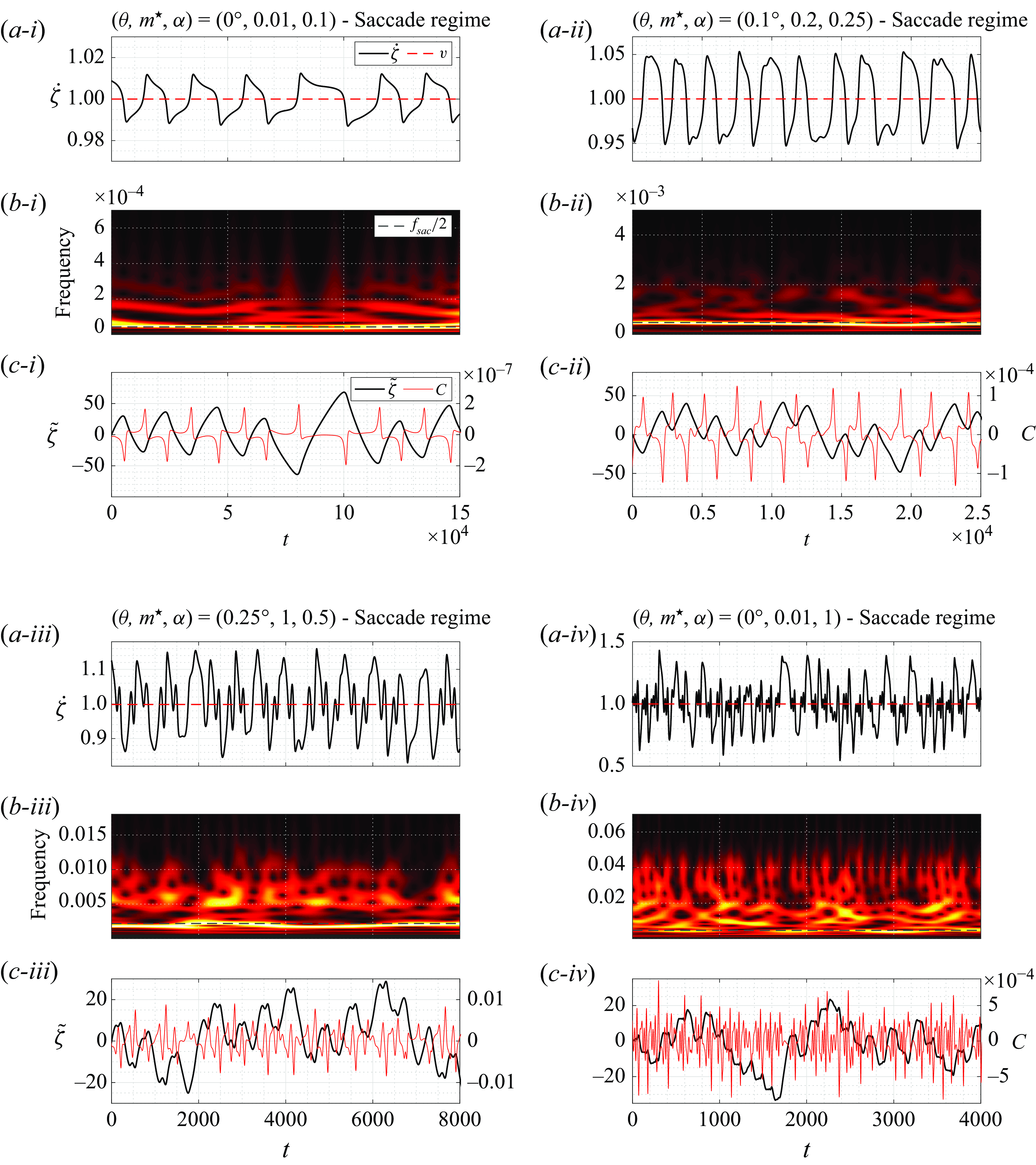
Figure 8. Selected time series of the cylinder (a) velocity, (b) velocity spectrum and (c) displacement fluctuation about its linear component, in typical cases of the second oscillation region (saccade regime), for (i) $(\theta ,m^\star ,\alpha )=(0^\circ ,0.01,0.1)$
, (ii)
$(\theta ,m^\star ,\alpha )=(0^\circ ,0.01,0.1)$
, (ii) $(\theta ,m^\star ,\alpha )=(0.1^\circ ,0.2,0.25)$
, (iii)
$(\theta ,m^\star ,\alpha )=(0.1^\circ ,0.2,0.25)$
, (iii) $(\theta ,m^\star ,\alpha )=(0.25^\circ ,1,0.5)$
and (iv)
$(\theta ,m^\star ,\alpha )=(0.25^\circ ,1,0.5)$
and (iv) $(\theta ,m^\star ,\alpha )=(0^\circ ,0.01,1)$
. The drift velocity (
$(\theta ,m^\star ,\alpha )=(0^\circ ,0.01,1)$
. The drift velocity ( $v$
) is superimposed on the time series in (a). In (b), the instantaneous spectral amplitude is normalised by its maximum value and the colour levels range from
$v$
) is superimposed on the time series in (a). In (b), the instantaneous spectral amplitude is normalised by its maximum value and the colour levels range from $0$
(black) to
$0$
(black) to $1$
(yellow); a grey dashed line indicates half of the saccade frequency. In (c), the displacement fluctuation is plotted together with the tangential force coefficient.
$1$
(yellow); a grey dashed line indicates half of the saccade frequency. In (c), the displacement fluctuation is plotted together with the tangential force coefficient.
The second oscillation region is limited to configurations where the direction of motion is aligned or almost aligned with the oncoming flow, i.e. $\theta \approx 0^\circ$
. Body oscillation appears to be triggered by the rotation as no fluctuation of the displacement occurs for
$\theta \approx 0^\circ$
. Body oscillation appears to be triggered by the rotation as no fluctuation of the displacement occurs for $\alpha =0$
. The oscillation region extends from a threshold value of the rotation rate located between
$\alpha =0$
. The oscillation region extends from a threshold value of the rotation rate located between $0.025$
and
$0.025$
and $0.05$
, to the largest value studied in this work (
$0.05$
, to the largest value studied in this work ( $\alpha =1$
). Its extension along the
$\alpha =1$
). Its extension along the $\theta$
axis slightly increases with
$\theta$
axis slightly increases with $\alpha$
, up to
$\alpha$
, up to $\theta \approx 0.5^\circ$
for
$\theta \approx 0.5^\circ$
for $\alpha =1$
. In contrast to the VIV region, its boundary in the
$\alpha =1$
. In contrast to the VIV region, its boundary in the $(\theta ,\alpha )$
domain does not depend on
$(\theta ,\alpha )$
domain does not depend on $m^\star$
, over the range investigated.
$m^\star$
, over the range investigated.
For $\theta \approx 0^\circ$
, the drift velocity (time-averaged velocity of the body) matches the oncoming flow velocity or is very close to it (
$\theta \approx 0^\circ$
, the drift velocity (time-averaged velocity of the body) matches the oncoming flow velocity or is very close to it ( $v\approx 1$
). The drift velocity is superimposed on
$v\approx 1$
). The drift velocity is superimposed on $\dot \zeta$
time series in figure 8(a). The effective flow seen by the body tends to vanish and the effective configuration essentially corresponds to the problem of a rotating cylinder immersed in quiescent fluid. Such a configuration cannot be rigorously considered through the above subcritical/postcritical condition prism, since there is no cross-current. Yet, the flow developing in the quiescent fluid problem remains steady when the rotating body is rigidly mounted, i.e. no flow unsteadiness exists without structural oscillation. In the absence of effective flow and associated velocity scale, the dynamics is expected to scale with the cylinder surface velocity (
$\dot \zeta$
time series in figure 8(a). The effective flow seen by the body tends to vanish and the effective configuration essentially corresponds to the problem of a rotating cylinder immersed in quiescent fluid. Such a configuration cannot be rigorously considered through the above subcritical/postcritical condition prism, since there is no cross-current. Yet, the flow developing in the quiescent fluid problem remains steady when the rotating body is rigidly mounted, i.e. no flow unsteadiness exists without structural oscillation. In the absence of effective flow and associated velocity scale, the dynamics is expected to scale with the cylinder surface velocity ( $\Omega D/2$
), which represents the only reference velocity in this case. Moreover, a Reynolds number based on the surface velocity (
$\Omega D/2$
), which represents the only reference velocity in this case. Moreover, a Reynolds number based on the surface velocity ( ${ Re}_{\scriptscriptstyle \Omega }=\rho _f\Omega D^2/(2\mu )$
) may be more relevant than Re or
${ Re}_{\scriptscriptstyle \Omega }=\rho _f\Omega D^2/(2\mu )$
) may be more relevant than Re or ${ Re}_{{eff}}$
to characterise the system condition. This Reynolds number is equal to
${ Re}_{{eff}}$
to characterise the system condition. This Reynolds number is equal to $\alpha { Re}$
and thus proportional to the rotation rate.
$\alpha { Re}$
and thus proportional to the rotation rate.
In the second oscillation region, the displacement of the body about its drifting motion can be qualitatively described as a series of erratic jumps of variable amplitudes, either upstream or downstream and, sometimes, repeatedly in the same direction (e.g. for $t\in [1000,1600]$
in figure 8
c-iv). Such an aperiodic evolution contrasts with the periodic and nearly sinusoidal nature of the VIV encountered at higher incidence. The successive jumps of the cylinder are referred to as ‘saccades’. This term is chosen to emphasise the irregular and jerky behaviour of the body, as opposed to the regularity of VIV. The corresponding region of the parameter space is named ‘saccade region’. Within the saccade region, pronounced modulations are already observed for low
$t\in [1000,1600]$
in figure 8
c-iv). Such an aperiodic evolution contrasts with the periodic and nearly sinusoidal nature of the VIV encountered at higher incidence. The successive jumps of the cylinder are referred to as ‘saccades’. This term is chosen to emphasise the irregular and jerky behaviour of the body, as opposed to the regularity of VIV. The corresponding region of the parameter space is named ‘saccade region’. Within the saccade region, pronounced modulations are already observed for low $\alpha$
(
$\alpha$
( $\alpha =0.1$
in figure 8
i) but the irregularity of the response tends to increase with the rotation rate. As
$\alpha =0.1$
in figure 8
i) but the irregularity of the response tends to increase with the rotation rate. As $\alpha$
is increased, relatively well-defined plateaus of
$\alpha$
is increased, relatively well-defined plateaus of $\tilde \zeta$
appear between the saccades. During these phases of stabilisation, the body exhibits secondary oscillations of lower amplitudes. This phenomenon, particularly visible for
$\tilde \zeta$
appear between the saccades. During these phases of stabilisation, the body exhibits secondary oscillations of lower amplitudes. This phenomenon, particularly visible for $\alpha \geqslant 0.5$
(figure 8
iii,iv), introduces additional scales in the response and participates in its increasing irregularity. Frequency modulations and the progressive emergence of additional components in the response spectrum, as
$\alpha \geqslant 0.5$
(figure 8
iii,iv), introduces additional scales in the response and participates in its increasing irregularity. Frequency modulations and the progressive emergence of additional components in the response spectrum, as $\alpha$
is increased, are visualised in figure 8(b), where a time-frequency representation (scalogram) of the cylinder velocity, based on wavelet transform of
$\alpha$
is increased, are visualised in figure 8(b), where a time-frequency representation (scalogram) of the cylinder velocity, based on wavelet transform of $\dot \zeta{-}v$
time series, is plotted for each selected case.
$\dot \zeta{-}v$
time series, is plotted for each selected case.
In the saccade region, due to the aperiodic and modulated dynamics of the body, the quantification of the oscillation properties requires a specific methodology. To measure the oscillation amplitude, the root-mean-square (r.m.s.) value of the displacement fluctuation is preferred to its maximum value, which may be too sensitive to rare events. The same approach is adopted to measure the amplitude of body velocity fluctuation. Fourier transform of the time series and time-averaged scalograms result in broadband spectra without clear dominant frequency, especially in the higher- $\alpha$
range. An alternative is proposed, based on the number of saccades. Each saccade is associated with a peak of magnitude of the body velocity fluctuation (
$\alpha$
range. An alternative is proposed, based on the number of saccades. Each saccade is associated with a peak of magnitude of the body velocity fluctuation ( $|\dot \zeta -v|$
). The saccade frequency,
$|\dot \zeta -v|$
). The saccade frequency, $f_{{sac}}$
, is defined as the number of these peaks exceeding a certain threshold, usually half of the averaged top
$f_{{sac}}$
, is defined as the number of these peaks exceeding a certain threshold, usually half of the averaged top $10\,\%$
peaks, divided by the duration of the sampling period. For a sinusoidal displacement, where two velocity peaks are observed per oscillation period,
$10\,\%$
peaks, divided by the duration of the sampling period. For a sinusoidal displacement, where two velocity peaks are observed per oscillation period, $f_{{sac}}$
is equal to twice the Fourier transform frequency. For comparison, half of
$f_{{sac}}$
is equal to twice the Fourier transform frequency. For comparison, half of $f_{{sac}}$
is superimposed on the scalograms in figure 8(b) (grey dashed line). It globally coincides with a salient (yet fluctuating) low-frequency component, which can be regarded as the trace of the saccades in the scalograms.
$f_{{sac}}$
is superimposed on the scalograms in figure 8(b) (grey dashed line). It globally coincides with a salient (yet fluctuating) low-frequency component, which can be regarded as the trace of the saccades in the scalograms.

Figure 9. (a) Oscillation amplitude, (b) velocity fluctuation amplitude and (c) saccade frequency, as functions of the rotation rate, in the saccade region. The amplitudes are quantified via the r.m.s. values of the displacement and velocity fluctuations. The ensemble average of all the available results (i.e. for $m^\star \in [0.01,1]$
and
$m^\star \in [0.01,1]$
and $\theta \approx 0^\circ$
) is represented for each
$\theta \approx 0^\circ$
) is represented for each $\alpha$
, and the shaded area visualises the standard deviation. In (b,c), the velocity fluctuation amplitude and saccade frequency are normalised by the rotation rate. Red dots denote the values measured in the four cases considered in figure 8. A light red dotted line indicates the trend identified in the lower-
$\alpha$
, and the shaded area visualises the standard deviation. In (b,c), the velocity fluctuation amplitude and saccade frequency are normalised by the rotation rate. Red dots denote the values measured in the four cases considered in figure 8. A light red dotted line indicates the trend identified in the lower- $\alpha$
range based on a limited number of simulations.
$\alpha$
range based on a limited number of simulations.
Some statistics of the cylinder dynamics in the saccade region are presented in figure 9, as functions of the rotation rate. For each $\alpha$
, the dynamics properties only exhibit a small dispersion when
$\alpha$
, the dynamics properties only exhibit a small dispersion when $m^\star$
and
$m^\star$
and $\theta$
are varied, and no trend emerges as a function of these parameters. That is why the ensemble average of all the available results (denoted by
$\theta$
are varied, and no trend emerges as a function of these parameters. That is why the ensemble average of all the available results (denoted by $\langle \rangle$
) is plotted for each
$\langle \rangle$
) is plotted for each $\alpha$
in figure 9. The dispersion about the average value is visualised by a shaded area that represents the standard deviation. Red dots denote the values measured in the cases depicted in figure 8. The trends identified in the lower-
$\alpha$
in figure 9. The dispersion about the average value is visualised by a shaded area that represents the standard deviation. Red dots denote the values measured in the cases depicted in figure 8. The trends identified in the lower- $\alpha$
range, based on a limited number of simulations (two to four, due to the very large time scales of the dynamics), are indicated by light red dotted lines.
$\alpha$
range, based on a limited number of simulations (two to four, due to the very large time scales of the dynamics), are indicated by light red dotted lines.
The order of magnitude of the oscillation amplitude is considerably larger than in the VIV region (figure 9
a). It tends to decrease as $\alpha$
is increased and stabilises close to
$\alpha$
is increased and stabilises close to $10D$
beyond
$10D$
beyond $\alpha =0.5$
, or, equivalently,
$\alpha =0.5$
, or, equivalently, ${ Re}_{\scriptscriptstyle \Omega }=50$
. To assess the possible scaling of the system dynamics with the cylinder surface velocity, the amplitude of body velocity fluctuation and the saccade frequency are normalised by
${ Re}_{\scriptscriptstyle \Omega }=50$
. To assess the possible scaling of the system dynamics with the cylinder surface velocity, the amplitude of body velocity fluctuation and the saccade frequency are normalised by $\alpha$
in figure 9(b,c). The normalised quantities increase with
$\alpha$
in figure 9(b,c). The normalised quantities increase with $\alpha$
and reach a plateau for
$\alpha$
and reach a plateau for $\alpha \gt 0.5$
, as also noted for the oscillation amplitude. As a result, beyond a certain
$\alpha \gt 0.5$
, as also noted for the oscillation amplitude. As a result, beyond a certain $\alpha$
threshold, the oscillation frequency (based on
$\alpha$
threshold, the oscillation frequency (based on $f_{{sac}}$
) tends to grow linearly with the rotation rate. An increasing trend of the oscillation frequency with
$f_{{sac}}$
) tends to grow linearly with the rotation rate. An increasing trend of the oscillation frequency with $\alpha$
, even though less steep, is also observed, at a fixed incidence angle, in the VIV region. This trend is however driven by the growth of
$\alpha$
, even though less steep, is also observed, at a fixed incidence angle, in the VIV region. This trend is however driven by the growth of $V_{{eff}}$
with
$V_{{eff}}$
with $\alpha$
(
$\alpha$
( $f_\zeta \approx { St} V_{{eff}}$
), while
$f_\zeta \approx { St} V_{{eff}}$
), while $V_{{eff}}$
vanishes in the saccade region, regardless of
$V_{{eff}}$
vanishes in the saccade region, regardless of $\alpha$
. Within the saccade region, the oscillation frequency remains one or more orders of magnitude lower than in the VIV region.
$\alpha$
. Within the saccade region, the oscillation frequency remains one or more orders of magnitude lower than in the VIV region.
Two supplementary points can be noted based on additional simulations. First, over the $\alpha$
range under study, the oscillation of the cylinder disappears when a second degree of freedom is added, i.e. when the body is free to move in the
$\alpha$
range under study, the oscillation of the cylinder disappears when a second degree of freedom is added, i.e. when the body is free to move in the $(x,y)$
plane. Without SRF, the restriction of body motion thus seems to be an important factor for the emergence of both VIV and saccades. Second, body oscillation persists when structural damping is introduced. As explained by Govardhan & Williamson (Reference Govardhan and Williamson2002), the absence of SRF may render the definition of a damping ratio rather arbitrary. Here,
$(x,y)$
plane. Without SRF, the restriction of body motion thus seems to be an important factor for the emergence of both VIV and saccades. Second, body oscillation persists when structural damping is introduced. As explained by Govardhan & Williamson (Reference Govardhan and Williamson2002), the absence of SRF may render the definition of a damping ratio rather arbitrary. Here, $f_\zeta$
and
$f_\zeta$
and $f_{{sac}}/2$
(measured without damping) are considered as references to define the critical damping in VIV and saccade cases. Both forms of response develop for damped systems. In particular, saccades comparable to those depicted in figure 8(iv) are observed, for
$f_{{sac}}/2$
(measured without damping) are considered as references to define the critical damping in VIV and saccade cases. Both forms of response develop for damped systems. In particular, saccades comparable to those depicted in figure 8(iv) are observed, for $\theta =0^\circ$
,
$\theta =0^\circ$
, $m^\star \in \{0.01,1\}$
and
$m^\star \in \{0.01,1\}$
and $\alpha =1$
, when the damping ratio is set to
$\alpha =1$
, when the damping ratio is set to $20\,\%$
.
$20\,\%$
.
To summarise, the cylinder exhibits two contrasted forms of oscillation, which develop in distinct conditions. Vortex-induced vibrations, close to sinusoidal, occur when the body is exposed to an effective flow, over a wide range of incidence angles and for all $\alpha$
. On the other hand, irregular jumps of the body, referred to as saccades, emerge close to
$\alpha$
. On the other hand, irregular jumps of the body, referred to as saccades, emerge close to $\theta =0^\circ$
, where the effective flow vanishes, and beyond a certain rotation rate. Contrary to VIV, the structural dynamics is insensitive to the value of the mass ratio in the saccade region. The two forms of response differ by their regularity, but also by their amplitude and frequency ranges. Saccades typically reach
$\theta =0^\circ$
, where the effective flow vanishes, and beyond a certain rotation rate. Contrary to VIV, the structural dynamics is insensitive to the value of the mass ratio in the saccade region. The two forms of response differ by their regularity, but also by their amplitude and frequency ranges. Saccades typically reach $10$
body diameters while VIV do not exceed half a diameter. An increase of the rotation rate tends to reduce the amplitude of both VIV and saccades. Yet, it enhances the erratic nature of the latter. The flow–body interaction mechanisms at play in these two forms of oscillation are examined in the next section.
$10$
body diameters while VIV do not exceed half a diameter. An increase of the rotation rate tends to reduce the amplitude of both VIV and saccades. Yet, it enhances the erratic nature of the latter. The flow–body interaction mechanisms at play in these two forms of oscillation are examined in the next section.
3.3. Interaction mechanisms
Within the parameter space investigated, the cylinder may either translate at a constant velocity without fluctuation of its displacement or exhibit an oscillation about its drifting motion. Based on the cylinder behaviour, the corresponding states of the system are referred to as ‘pure drift’ and ‘oscillatory’ regimes, respectively. The two forms of structural oscillation identified in § 3.2 are used to distinguish two oscillatory regimes, the VIV regime and the saccade regime. The distribution of the different regimes in the $(\theta ,\alpha )$
domain is visualised in figure 10. As previously mentioned, the frontier between the pure drift and saccade regimes appears to be independent of
$(\theta ,\alpha )$
domain is visualised in figure 10. As previously mentioned, the frontier between the pure drift and saccade regimes appears to be independent of $m^\star$
, which is not the case of the transition with the VIV regime. The transition region is depicted by a striped area and the progressive displacement of the frontier towards higher
$m^\star$
, which is not the case of the transition with the VIV regime. The transition region is depicted by a striped area and the progressive displacement of the frontier towards higher $\theta$
, as
$\theta$
, as $m^\star$
is increased, is indicated by a dashed arrow. The location of the critical conditions (
$m^\star$
is increased, is indicated by a dashed arrow. The location of the critical conditions ( ${ Re}_{{eff}}$
and
${ Re}_{{eff}}$
and $\alpha _{{eff}}$
) is denoted by a blue dashed line. It delimits the region of subcritical VIV.
$\alpha _{{eff}}$
) is denoted by a blue dashed line. It delimits the region of subcritical VIV.
The principal properties of the flow in the three regimes of the system are described in § 3.3.1. Some elements concerning fluid forcing are reported in § 3.3.2. Finally, in § 3.3.3, the present system behaviour is discussed, via an analogy with the system with SRF, in light of the evolution of the added mass with the effective conditions.
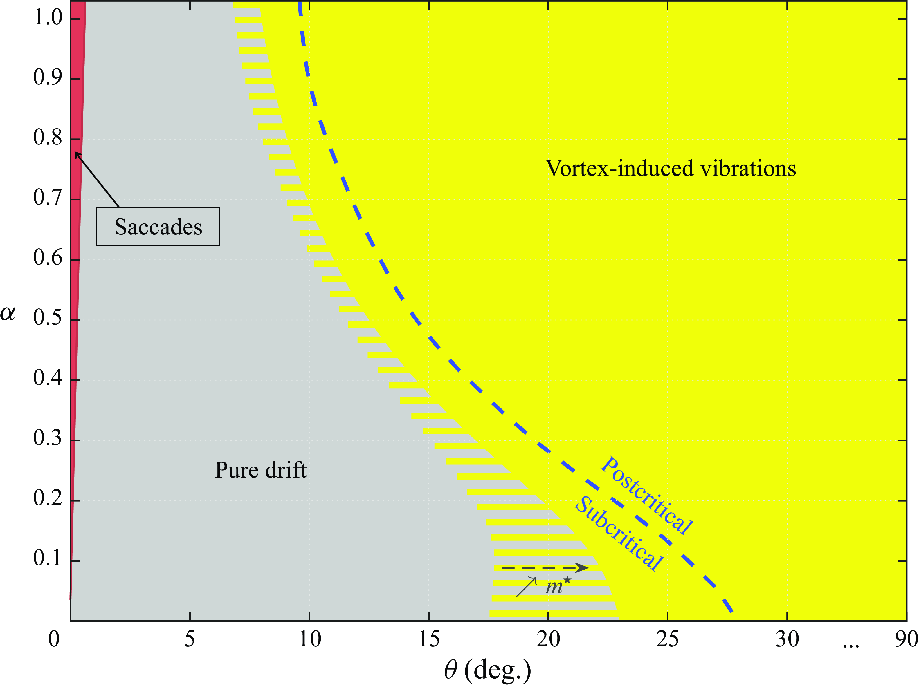
Figure 10. Flow–body system regime as a function of the incidence angle and rotation rate. To facilitate the visualisation of the different regimes, the $\theta$
axis range is discontinuous. The grey/yellow striped area depicts the evolution of the frontier between the pure drift and VIV regimes as the mass ratio is varied from
$\theta$
axis range is discontinuous. The grey/yellow striped area depicts the evolution of the frontier between the pure drift and VIV regimes as the mass ratio is varied from $0.01$
to
$0.01$
to $1$
; the displacement of this frontier towards higher
$1$
; the displacement of this frontier towards higher $\theta$
as
$\theta$
as $m^\star$
is increased is denoted by a dashed arrow. A blue dashed line delimits the subcritical and postcritical regions.
$m^\star$
is increased is denoted by a dashed arrow. A blue dashed line delimits the subcritical and postcritical regions.
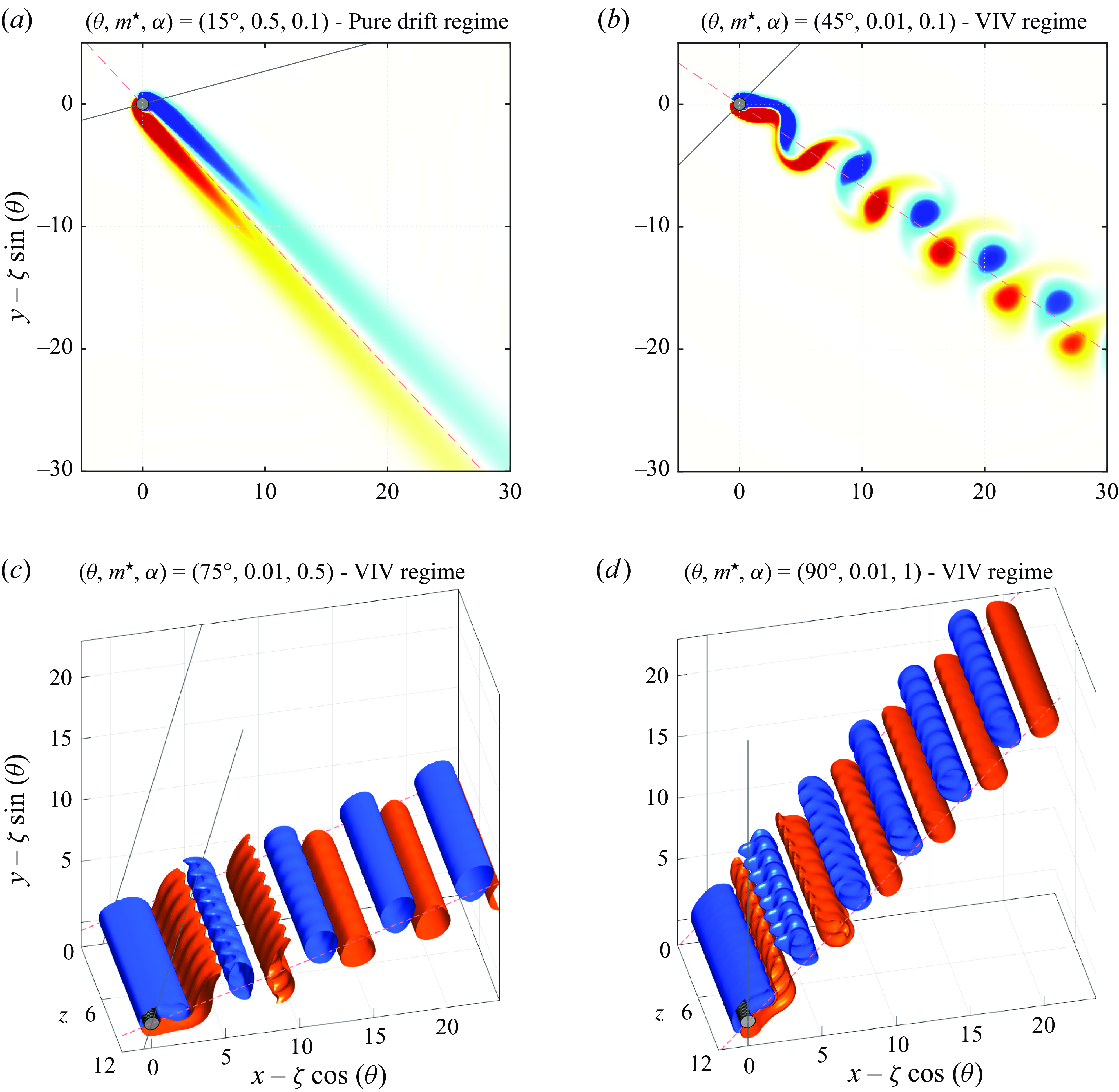
Figure 11. Instantaneous (a,b) iso-contours and (c,d) iso-surfaces of spanwise vorticity, for (a) $(\theta ,m^\star ,\alpha )=(15^\circ ,0.5,0.1)$
(pure drift regime), (b)
$(\theta ,m^\star ,\alpha )=(15^\circ ,0.5,0.1)$
(pure drift regime), (b) $(\theta ,m^\star ,\alpha )=(45^\circ ,0.01,0.1)$
(VIV regime), (c)
$(\theta ,m^\star ,\alpha )=(45^\circ ,0.01,0.1)$
(VIV regime), (c) $(\theta ,m^\star ,\alpha )=(75^\circ ,0.01,0.5)$
(VIV regime) and (d)
$(\theta ,m^\star ,\alpha )=(75^\circ ,0.01,0.5)$
(VIV regime) and (d) $(\theta ,m^\star ,\alpha )=(90^\circ ,0.01,1)$
(VIV regime);
$(\theta ,m^\star ,\alpha )=(90^\circ ,0.01,1)$
(VIV regime); $\omega _z\in [-0.5 V_{{eff}},0.5 V_{{eff}}]$
in (a,b) and
$\omega _z\in [-0.5 V_{{eff}},0.5 V_{{eff}}]$
in (a,b) and $\omega _z=\pm 0.2 V_{{eff}}$
in (c,d). Positive/negative vorticity values are plotted in red/blue. The frame is centred about the instantaneous position of the cylinder. Its trajectory is indicated by grey solid lines. The direction of the effective flow seen by the body is visualised by red dashed lines. Part of the computational domain is shown.
$\omega _z=\pm 0.2 V_{{eff}}$
in (c,d). Positive/negative vorticity values are plotted in red/blue. The frame is centred about the instantaneous position of the cylinder. Its trajectory is indicated by grey solid lines. The direction of the effective flow seen by the body is visualised by red dashed lines. Part of the computational domain is shown.
3.3.1. Flow physics
In the pure drift regime, the instantaneous flow seen by the cylinder is steady. Close to $\theta = 0^\circ$
,
$\theta = 0^\circ$
, $V_{{eff}}$
vanishes and the configuration becomes similar to the case of a cylinder immersed in quiescent fluid. For
$V_{{eff}}$
vanishes and the configuration becomes similar to the case of a cylinder immersed in quiescent fluid. For $\alpha \gt 0$
, the flow surrounding the cylinder is principally composed of an axisymmetric zone of negative vorticity (due to the counter-clockwise rotation), whose magnitude progressively decreases away from the body. At higher incidence, when the effective flow is sufficiently intense for a wake to develop, its organisation remains close to the pattern visualised in figure 11(a) by instantaneous iso-contours of spanwise vorticity (
$\alpha \gt 0$
, the flow surrounding the cylinder is principally composed of an axisymmetric zone of negative vorticity (due to the counter-clockwise rotation), whose magnitude progressively decreases away from the body. At higher incidence, when the effective flow is sufficiently intense for a wake to develop, its organisation remains close to the pattern visualised in figure 11(a) by instantaneous iso-contours of spanwise vorticity ( $\omega _z$
). In this figure, the rectilinear path and the direction of the effective flow are indicated by grey solid and red dashed lines, respectively. The imposed rotation induces an asymmetry in the shapes and magnitudes of the elongated layers of positive and negative vorticity forming in the wake of the drifting body.
$\omega _z$
). In this figure, the rectilinear path and the direction of the effective flow are indicated by grey solid and red dashed lines, respectively. The imposed rotation induces an asymmetry in the shapes and magnitudes of the elongated layers of positive and negative vorticity forming in the wake of the drifting body.
In the VIV regime, body oscillation and flow unsteadiness are synchronised. Such synchronisation is usually referred to as lock-in (Williamson & Govardhan Reference Williamson and Govardhan2004). The dominant frequency of flow unsteadiness, issued from the periodic time series of flow velocity sampled downstream of the body, always coincides with the oscillation frequency ( $f_\zeta$
). As a result, the oscillation frequency plots in figure 6(b) also represent the evolution of flow unsteadiness frequency across the VIV region of the parameter space. As previously noted for the oscillation frequency, flow unsteadiness frequency does not substantially depart from the Strouhal frequency associated with the wake of a rigidly mounted cylinder placed in cross-current; the ratio with respect to St ranges from
$f_\zeta$
). As a result, the oscillation frequency plots in figure 6(b) also represent the evolution of flow unsteadiness frequency across the VIV region of the parameter space. As previously noted for the oscillation frequency, flow unsteadiness frequency does not substantially depart from the Strouhal frequency associated with the wake of a rigidly mounted cylinder placed in cross-current; the ratio with respect to St ranges from $0.8$
to
$0.8$
to $1$
. Throughout the VIV region, two counter-rotating spanwise vortices form per oscillation period (
$1$
. Throughout the VIV region, two counter-rotating spanwise vortices form per oscillation period ( $1/f_\zeta$
). Following the nomenclature proposed by Williamson & Roshko (Reference Williamson and Roshko1988), this corresponds to the 2S pattern. As illustrated in figure 11(b) for a typical VIV case, the flow closely resembles the von Kármán street developing in the wake of a fixed cylinder. In the absence of rotation, the effective configuration remains symmetrical (
$1/f_\zeta$
). Following the nomenclature proposed by Williamson & Roshko (Reference Williamson and Roshko1988), this corresponds to the 2S pattern. As illustrated in figure 11(b) for a typical VIV case, the flow closely resembles the von Kármán street developing in the wake of a fixed cylinder. In the absence of rotation, the effective configuration remains symmetrical ( $\theta _{{eff}}=90^\circ$
, as explained in § 3.1) and a strict antisymmetry of the vortex shedding is preserved, regardless of
$\theta _{{eff}}=90^\circ$
, as explained in § 3.1) and a strict antisymmetry of the vortex shedding is preserved, regardless of $\theta$
. For
$\theta$
. For $\alpha \gt 0$
, the combination of body rotation and path inclination slightly perturbs this antisymmetry.
$\alpha \gt 0$
, the combination of body rotation and path inclination slightly perturbs this antisymmetry.
Even if the $({ Re}_{{eff}},\alpha _{{eff}})$
domain visited by the system does not include the threshold of the three-dimensional transition in the flow past a rigidly mounted cylinder (Rao et al. Reference Rao, Radi, Leontini, Thompson, Sheridan and Hourigan2015), the transition actually occurs under the effect of body oscillation. Such enhancement of the three-dimensional transition by body motion was previously reported for comparable systems involving a rotating cylinder with SRF (e.g. Bourguet Reference Bourguet2019). The flow is found to become three-dimensional at high incidence angles,
$({ Re}_{{eff}},\alpha _{{eff}})$
domain visited by the system does not include the threshold of the three-dimensional transition in the flow past a rigidly mounted cylinder (Rao et al. Reference Rao, Radi, Leontini, Thompson, Sheridan and Hourigan2015), the transition actually occurs under the effect of body oscillation. Such enhancement of the three-dimensional transition by body motion was previously reported for comparable systems involving a rotating cylinder with SRF (e.g. Bourguet Reference Bourguet2019). The flow is found to become three-dimensional at high incidence angles, $\theta \gt 60^\circ$
approximately, and for rotation rates larger than
$\theta \gt 60^\circ$
approximately, and for rotation rates larger than $0.4$
; it is recalled that Re
$0.4$
; it is recalled that Re $=100$
. These conditions roughly correspond to
$=100$
. These conditions roughly correspond to $\theta _{{eff}}\lt 60^\circ$
,
$\theta _{{eff}}\lt 60^\circ$
, ${ Re}_{{eff}}\gt 115$
and
${ Re}_{{eff}}\gt 115$
and $\alpha _{{eff}}\gt 0.35$
. At fixed
$\alpha _{{eff}}\gt 0.35$
. At fixed $\theta$
and
$\theta$
and $\alpha$
, the occurrence of the transition depends on the oscillation amplitude and frequency, and thus on
$\alpha$
, the occurrence of the transition depends on the oscillation amplitude and frequency, and thus on $m^\star$
. The region of the parameter space where the flow is three-dimensional is visualised by horizontal stripes in figures 6(a) and 7. Considering their dependence on the nominal/effective conditions, the objective here is not to determine the oscillation properties required to induce the transition. Yet, it can be noted that an amplitude of the order of
$m^\star$
. The region of the parameter space where the flow is three-dimensional is visualised by horizontal stripes in figures 6(a) and 7. Considering their dependence on the nominal/effective conditions, the objective here is not to determine the oscillation properties required to induce the transition. Yet, it can be noted that an amplitude of the order of $0.1D$
may be sufficient to trigger it.
$0.1D$
may be sufficient to trigger it.
Two examples representative of the three-dimensionality of the flow are visualised in figure 11(c,d), via instantaneous iso-surfaces of spanwise vorticity. The structure of the wake remains dominated by the alternating vortex shedding described above, i.e. the 2S pattern. The three-dimensional nature of the flow manifests by a regular spanwise undulation of the vortex rows in the near region. The undulation tends to vanish further in the wake where the spanwise vortex rows are mainly two-dimensional. The wavelength of the spanwise undulation ranges from $1.3D$
to
$1.3D$
to $1.5D$
. For a rigidly mounted cylinder, the wavelength observed at the onset of three-dimensionality at
$1.5D$
. For a rigidly mounted cylinder, the wavelength observed at the onset of three-dimensionality at ${ Re}_r=100$
, for
${ Re}_r=100$
, for $\alpha _r\approx 3.7$
, is
$\alpha _r\approx 3.7$
, is $1.7D$
approximately (Bourguet & Lo Jacono Reference Bourguet and Lo Jacono2014), while for
$1.7D$
approximately (Bourguet & Lo Jacono Reference Bourguet and Lo Jacono2014), while for $\alpha _r=0$
, the transition occurs at
$\alpha _r=0$
, the transition occurs at ${ Re}_r \approx 190$
with a wavelength close to
${ Re}_r \approx 190$
with a wavelength close to $4D$
(Williamson Reference Williamson1996). The dynamics of the three-dimensional flow is subharmonic, with a fundamental frequency equal to
$4D$
(Williamson Reference Williamson1996). The dynamics of the three-dimensional flow is subharmonic, with a fundamental frequency equal to $f_\zeta /2$
, versus
$f_\zeta /2$
, versus $f_\zeta$
in the two-dimensional case, even if the dominant component is still associated with
$f_\zeta$
in the two-dimensional case, even if the dominant component is still associated with $f_\zeta$
. Even though rather subtle, this subharmonic evolution is visible in figure 11(c,d): the spanwise undulation appears to be shifted by half a wavelength between two consecutive vortex rows of same vorticity sign. It can be verified by monitoring the time series of the sectional fluid forces along the span, as shown in Bourguet (Reference Bourguet2020), where a similar subharmonic evolution was reported for a system with SRF. The subharmonic component vanishes from the span-averaged force spectra. The fact that the flow is principally structured by the two-dimensional vortex shedding pattern suggests a limited influence of its three-dimensionality on fluid forcing and body response. This is actually the case, as illustrated in figure 3(iii) (green dotted lines). Assuming that the flow is two-dimensional results in a slight overestimation of the oscillation amplitude, but the difference is small, typically lower than
$f_\zeta$
. Even though rather subtle, this subharmonic evolution is visible in figure 11(c,d): the spanwise undulation appears to be shifted by half a wavelength between two consecutive vortex rows of same vorticity sign. It can be verified by monitoring the time series of the sectional fluid forces along the span, as shown in Bourguet (Reference Bourguet2020), where a similar subharmonic evolution was reported for a system with SRF. The subharmonic component vanishes from the span-averaged force spectra. The fact that the flow is principally structured by the two-dimensional vortex shedding pattern suggests a limited influence of its three-dimensionality on fluid forcing and body response. This is actually the case, as illustrated in figure 3(iii) (green dotted lines). Assuming that the flow is two-dimensional results in a slight overestimation of the oscillation amplitude, but the difference is small, typically lower than $15\,\%$
. That is why, as previously mentioned, the two-dimensional simulation results appear to be sufficiently accurate to describe the global trends of the system behaviour.
$15\,\%$
. That is why, as previously mentioned, the two-dimensional simulation results appear to be sufficiently accurate to describe the global trends of the system behaviour.
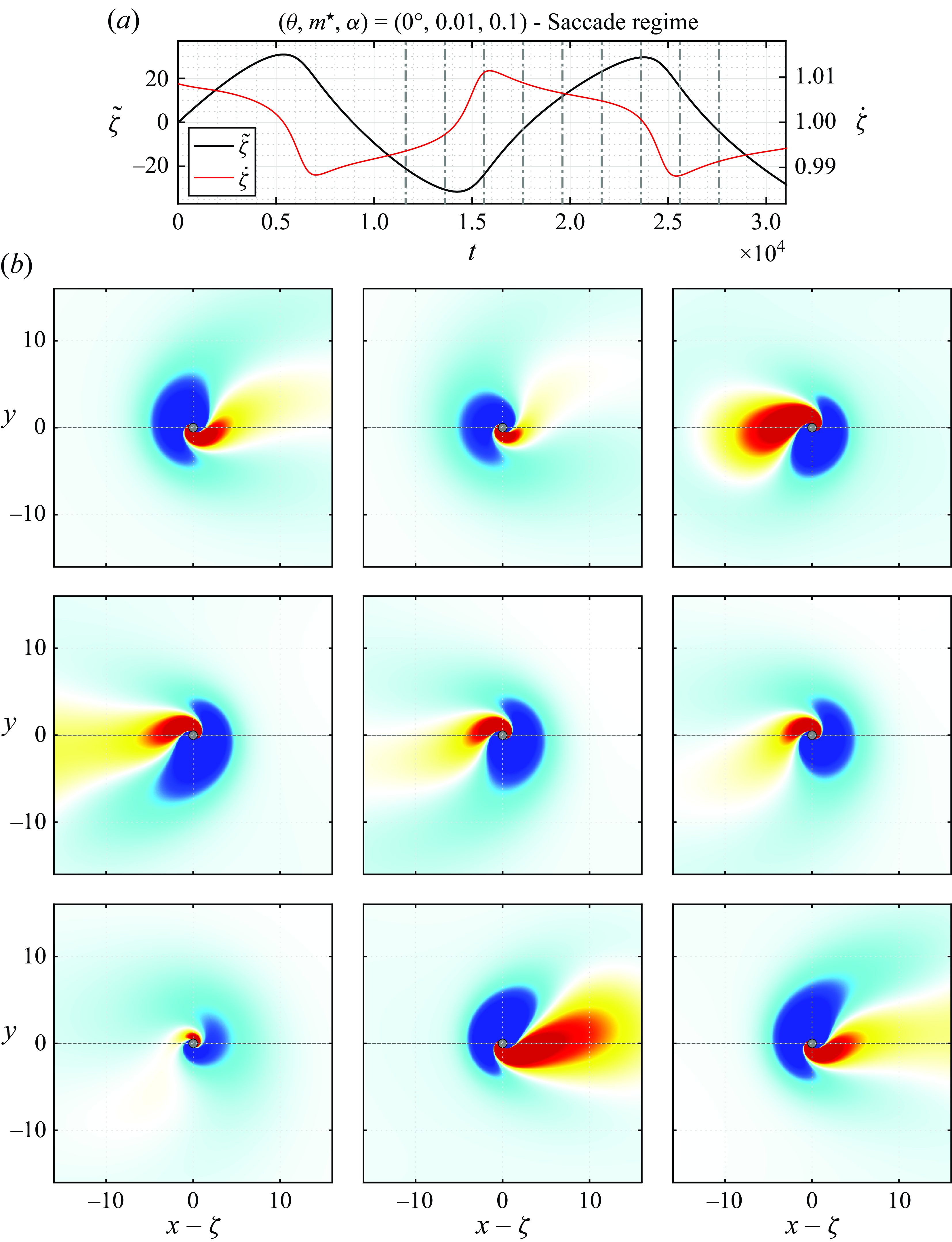
Figure 12. (a) Selected time series of the cylinder displacement fluctuation and velocity, and (b) instantaneous iso-contours of spanwise vorticity ( $\omega _z\in [-0.001,0.001]$
), for
$\omega _z\in [-0.001,0.001]$
), for $(\theta ,m^\star ,\alpha )=(0^\circ ,0.01,0.1)$
(saccade regime). Positive/negative vorticity values are plotted in red/blue. The successive instants visualised in (b) are indicated by grey dash-dotted lines in (a). Each frame is centred about the instantaneous position of the cylinder. Its trajectory is represented by a grey solid line. Part of the computational domain is shown.
$(\theta ,m^\star ,\alpha )=(0^\circ ,0.01,0.1)$
(saccade regime). Positive/negative vorticity values are plotted in red/blue. The successive instants visualised in (b) are indicated by grey dash-dotted lines in (a). Each frame is centred about the instantaneous position of the cylinder. Its trajectory is represented by a grey solid line. Part of the computational domain is shown.
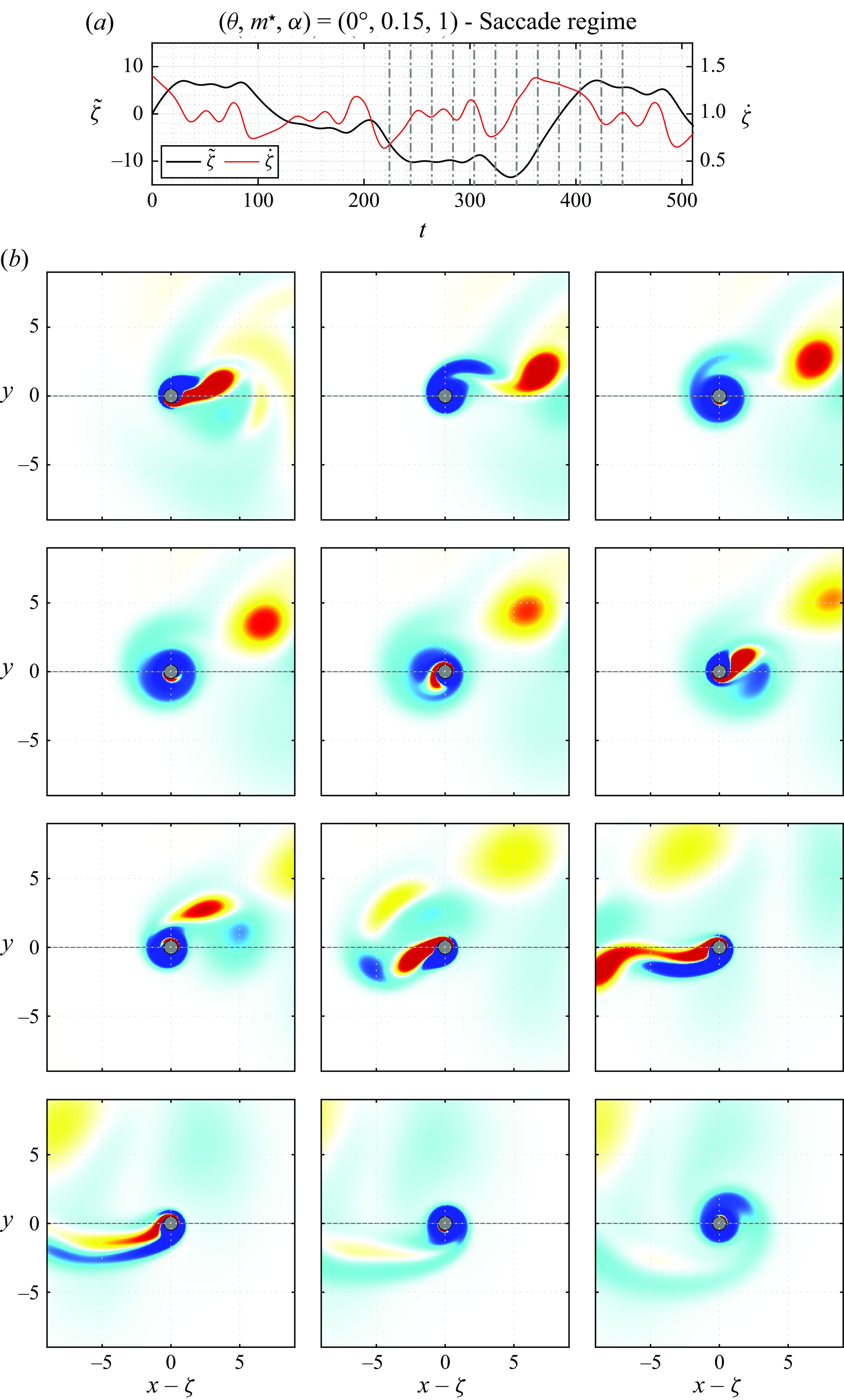
Figure 13. Same as figure 12 for $(\theta ,m^\star ,\alpha )=(0^\circ ,0.15,1)$
,
$(\theta ,m^\star ,\alpha )=(0^\circ ,0.15,1)$
, $\omega _z\in [-0.1,0.1]$
(saccade regime).
$\omega _z\in [-0.1,0.1]$
(saccade regime).
The saccade regime develops in an effective configuration where, if the cylinder is rigidly mounted, the flow is steady. When the cylinder is free to translate, body oscillation and flow unsteadiness arise simultaneously. To visualise the organisation of the flow and its coupling with body motion, two series of snapshots of instantaneous spanwise vorticity, captured for $\theta =0^\circ$
,
$\theta =0^\circ$
, $\alpha =0.1$
and
$\alpha =0.1$
and $\alpha =1$
, are plotted in figures 12 and 13, respectively. The sampling instants are indicated in the time series of the body displacement fluctuation and velocity, above the snapshots. The selected cases encompass the
$\alpha =1$
, are plotted in figures 12 and 13, respectively. The sampling instants are indicated in the time series of the body displacement fluctuation and velocity, above the snapshots. The selected cases encompass the $\alpha$
range of the saccade region. The axisymmetric, steady flow pattern is considerably altered once the cylinder oscillates, with the emergence of unsteady vortical structures of both signs. The increasing trend of the oscillation frequency with
$\alpha$
range of the saccade region. The axisymmetric, steady flow pattern is considerably altered once the cylinder oscillates, with the emergence of unsteady vortical structures of both signs. The increasing trend of the oscillation frequency with $\alpha$
(figure 9
c) is accompanied by a global reduction of the size of the vortical structures. For
$\alpha$
(figure 9
c) is accompanied by a global reduction of the size of the vortical structures. For $\alpha =0.1$
, their large scale, of the order of
$\alpha =0.1$
, their large scale, of the order of $10D$
, is reminiscent of the vortices composing the wake of a cylinder with SRF subjected to FIV of comparable amplitudes, at a Reynolds number of
$10D$
, is reminiscent of the vortices composing the wake of a cylinder with SRF subjected to FIV of comparable amplitudes, at a Reynolds number of $5$
or
$5$
or $10$
(Bourguet Reference Bourguet2023b
). The vortical structures observed for
$10$
(Bourguet Reference Bourguet2023b
). The vortical structures observed for $\alpha =1$
are more commensurable with those encountered in the present VIV region, even though still larger. No three-dimensional transition of the flow was detected within the saccade region.
$\alpha =1$
are more commensurable with those encountered in the present VIV region, even though still larger. No three-dimensional transition of the flow was detected within the saccade region.
The flow dynamics globally consists of an undulation, synchronised with body motion, of the vorticity layers wrapped around the cylinder. In addition, elongated zones of vorticity can be noted downstream of the body during the large fluctuations of its displacement, with the formation and detachment of distinct vortices in the higher- $\alpha$
case (figure 13). A comparison of the snapshots captured for
$\alpha$
case (figure 13). A comparison of the snapshots captured for $\alpha =0.1$
and
$\alpha =0.1$
and $\alpha =1$
emphasises the increasing level of irregularity of the flow as
$\alpha =1$
emphasises the increasing level of irregularity of the flow as $\alpha$
is increased, which coincides with the amplification of the erratic character of the cylinder response reported in § 3.2.2. In that sense, the scalograms of body velocity in figure 8(b) are also representative of the flow frequency content and its evolution with
$\alpha$
is increased, which coincides with the amplification of the erratic character of the cylinder response reported in § 3.2.2. In that sense, the scalograms of body velocity in figure 8(b) are also representative of the flow frequency content and its evolution with $\alpha$
. During the plateaus of
$\alpha$
. During the plateaus of $\tilde \zeta$
appearing in the higher-
$\tilde \zeta$
appearing in the higher- $\alpha$
range, for example around
$\alpha$
range, for example around $t=250$
in figure 13, the negative vorticity layer surrounding the cylinder grows, and this growth is associated with the development of a slight undulation of both the body and the flow, which progressively intensifies. After a few undulation cycles, typically three for
$t=250$
in figure 13, the negative vorticity layer surrounding the cylinder grows, and this growth is associated with the development of a slight undulation of both the body and the flow, which progressively intensifies. After a few undulation cycles, typically three for $\alpha =1$
, a jump (saccade) of the body occurs. This phenomenon suggests that the vorticity layer wrapped around the rotating cylinder becomes unstable as it grows and that its destabilisation, triggered by the joint undulation of the body, causes the saccade. The disappearance of the plateaus of
$\alpha =1$
, a jump (saccade) of the body occurs. This phenomenon suggests that the vorticity layer wrapped around the rotating cylinder becomes unstable as it grows and that its destabilisation, triggered by the joint undulation of the body, causes the saccade. The disappearance of the plateaus of $\tilde \zeta$
in the lower-
$\tilde \zeta$
in the lower- $\alpha$
range can be linked to the perpetually unstable nature of the vorticity layers, i.e. absence of period of growth before possible destabilisation, perhaps in relation with their larger thickness compared with those observed for higher
$\alpha$
range can be linked to the perpetually unstable nature of the vorticity layers, i.e. absence of period of growth before possible destabilisation, perhaps in relation with their larger thickness compared with those observed for higher $\alpha$
, resulting in a continuous oscillation of the body. In all cases, the interplay of the rotating cylinder with flow unsteadiness, more precisely with the vorticity layers wrapped around it, appears to be a central element of the saccade regime. Since this regime develops in the absence of effective flow, the previously generated vortical structures remain in the vicinity of the cylinder during the subsequent oscillations. The interaction of the body with these persistent vortices could explain the irregularity of the saccade regime.
$\alpha$
, resulting in a continuous oscillation of the body. In all cases, the interplay of the rotating cylinder with flow unsteadiness, more precisely with the vorticity layers wrapped around it, appears to be a central element of the saccade regime. Since this regime develops in the absence of effective flow, the previously generated vortical structures remain in the vicinity of the cylinder during the subsequent oscillations. The interaction of the body with these persistent vortices could explain the irregularity of the saccade regime.
Despite their contrasted properties, VIV and saccades both involve a close connection between body motion and flow unsteadiness. Hereafter, this connection is investigated from the fluid force perspective.
3.3.2. Fluid forcing
Body oscillation is accompanied by an alteration of fluid forces compared with those exerted on a rigidly mounted cylinder in the same effective conditions. The effective flow vanishes in the saccade regime and the comparison focuses on the VIV regime. The amplification of the time-averaged force aligned with the effective flow, typically reported in this context (e.g. Khalak & Williamson Reference Khalak and Williamson1999), reaches $20\,\%$
. The Magnus effect is attenuated, but the reduction of the magnitude of the time-averaged force normal to the effective flow does not exceed
$20\,\%$
. The Magnus effect is attenuated, but the reduction of the magnitude of the time-averaged force normal to the effective flow does not exceed $10\,\%$
. Force alteration participates in the deviation of the actual drift velocity from its prediction via a quasi-steady model of the tangential force, which is based on the force coefficients measured in the rigidly mounted body case. Yet, as shown in § 3.1.1, the deviation remains small and the quasi-steady approach provides a relatively accurate estimate of the drift velocity. It is recalled that the drift velocity is also accurately predicted in the saccade regime. On the other hand, this modelling of the force fails to predict the emergence of VIV and saccades. This has been assessed by replacing the force coefficient
$10\,\%$
. Force alteration participates in the deviation of the actual drift velocity from its prediction via a quasi-steady model of the tangential force, which is based on the force coefficients measured in the rigidly mounted body case. Yet, as shown in § 3.1.1, the deviation remains small and the quasi-steady approach provides a relatively accurate estimate of the drift velocity. It is recalled that the drift velocity is also accurately predicted in the saccade regime. On the other hand, this modelling of the force fails to predict the emergence of VIV and saccades. This has been assessed by replacing the force coefficient $C$
on the right-hand side of the dynamics equation (2.2), originally issued from the unsteady flow simulation, by its quasi-steady model. Such a result is expected considering that the close connection of body motion and flow unsteadiness, emphasised in the previous section for both forms of response, is neglected in the quasi-steady approach.
$C$
on the right-hand side of the dynamics equation (2.2), originally issued from the unsteady flow simulation, by its quasi-steady model. Such a result is expected considering that the close connection of body motion and flow unsteadiness, emphasised in the previous section for both forms of response, is neglected in the quasi-steady approach.
The time series of the tangential force coefficient issued from the unsteady simulation is plotted together with the displacement fluctuation signal for each case depicted in figures 3 and 8. The tangential force remains equal to zero in the pure drift regime (figure 3
c-i). In the oscillatory regimes, the time-averaged value of $C$
vanishes and the magnitude of its fluctuation substantially varies across the parameter space. This variation is due to the range of
$C$
vanishes and the magnitude of its fluctuation substantially varies across the parameter space. This variation is due to the range of $m^\star$
investigated and to the diversity of the possible dynamics of the system, but also to the normalisation by the oncoming flow velocity (
$m^\star$
investigated and to the diversity of the possible dynamics of the system, but also to the normalisation by the oncoming flow velocity ( $U$
). The effective flow and body surface velocity magnitudes could be used to rescale the force coefficient in the different regions of the parameter space, via
$U$
). The effective flow and body surface velocity magnitudes could be used to rescale the force coefficient in the different regions of the parameter space, via $V_{{eff}}$
and
$V_{{eff}}$
and $\alpha$
. Here, to simplify the presentation, the normalisation is kept the same throughout the domain.
$\alpha$
. Here, to simplify the presentation, the normalisation is kept the same throughout the domain.
In the VIV regime, the tangential force is periodic and synchronised with body oscillation. As previously noted for the cylinder dynamics, the system exhibits a transverse symmetry for $\alpha =0$
, regardless of the incidence angle, and only odd harmonics appear in the
$\alpha =0$
, regardless of the incidence angle, and only odd harmonics appear in the $C$
spectrum. Even harmonics also arise when the symmetry is broken by the rotation. Without SRF and damping, for a periodic oscillation as those encountered in the VIV regime, the condition
$C$
spectrum. Even harmonics also arise when the symmetry is broken by the rotation. Without SRF and damping, for a periodic oscillation as those encountered in the VIV regime, the condition $m^\star \gt 0$
implies that the spectral components of
$m^\star \gt 0$
implies that the spectral components of $C$
and
$C$
and $\tilde \zeta$
are in phase opposition (Gsell et al. Reference Gsell, Bourguet and Braza2016). The phase opposition of force and displacement can be visualised in figure 3(c-ii,c-iii).
$\tilde \zeta$
are in phase opposition (Gsell et al. Reference Gsell, Bourguet and Braza2016). The phase opposition of force and displacement can be visualised in figure 3(c-ii,c-iii).
In the saccade regime, the force exhibits an aperiodic evolution and its irregularity increases with $\alpha$
, as also observed for the body dynamics. The equilibrium of the energy transfer between the flow and the body, i.e.
$\alpha$
, as also observed for the body dynamics. The equilibrium of the energy transfer between the flow and the body, i.e. $\overline {C\dot \zeta }=0$
in the absence of structural damping, is only reached over a long time interval, while it is achieved over each oscillation cycle (
$\overline {C\dot \zeta }=0$
in the absence of structural damping, is only reached over a long time interval, while it is achieved over each oscillation cycle ( $1/f_\zeta$
) in the VIV regime. Force-displacement phase opposition tends to persist in the saccade regime. This is particularly visible in the lower-
$1/f_\zeta$
) in the VIV regime. Force-displacement phase opposition tends to persist in the saccade regime. This is particularly visible in the lower- $\alpha$
range (figure 8
c-i,c-ii) but still discernible for higher
$\alpha$
range (figure 8
c-i,c-ii) but still discernible for higher $\alpha$
, including during the secondary oscillations occurring between the saccades (figure 3
c-iv).
$\alpha$
, including during the secondary oscillations occurring between the saccades (figure 3
c-iv).
The dynamics equation (2.2) implies that the added mass coefficient associated with the tangential force in phase with body acceleration, $C_m$
, is equal to the opposite of the mass ratio, regardless of the oscillation regime:
$C_m$
, is equal to the opposite of the mass ratio, regardless of the oscillation regime:
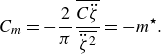 \begin{align} C_m=-\dfrac {2}{\pi }\dfrac {\overline {C\ddot \zeta }}{\overline {\ddot \zeta ^2}}=-m^\star . \end{align}
The added mass is further analysed in the next section, where it is used to link the behaviours of the systems with and without SRF.
3.3.3. Some insights from the system with SRF
To shed some light on the present system behaviour, an analogy with the trends observed when the cylinder is mounted on an elastic support is proposed here, following an approach introduced in Bourguet (Reference Bourguet2024). The elastic support adds a SRF and a structural natural frequency ( $f_n$
) to the system, as described in § 2.1. For a periodic oscillation with SRF, the partial added mass coefficient associated with the spectral components of
$f_n$
) to the system, as described in § 2.1. For a periodic oscillation with SRF, the partial added mass coefficient associated with the spectral components of $\tilde \zeta$
and
$\tilde \zeta$
and $C$
at the frequency
$C$
at the frequency $f_\zeta$
can be expressed as
$f_\zeta$
can be expressed as
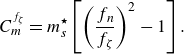 \begin{align} C^{\scriptscriptstyle f_\zeta }_m=m^\star _s\left [\left (\dfrac {f_n}{f_\zeta }\right )^2-1\right ]. \end{align}
It is recalled that $m^\star _s$
denotes the mass ratio in the system with SRF. The partial added mass coefficient is equal to the total added mass coefficient
$m^\star _s$
denotes the mass ratio in the system with SRF. The partial added mass coefficient is equal to the total added mass coefficient $C_m$
(3.6) for a sinusoidal response; without SRF,
$C_m$
(3.6) for a sinusoidal response; without SRF, $C^{\scriptscriptstyle f_\zeta }_m=C_m=-m^\star$
regardless of the presence of higher harmonics. Considering a sinusoidal oscillation at the frequency
$C^{\scriptscriptstyle f_\zeta }_m=C_m=-m^\star$
regardless of the presence of higher harmonics. Considering a sinusoidal oscillation at the frequency $f_\zeta$
, the same behaviour can occur with and without SRF when
$f_\zeta$
, the same behaviour can occur with and without SRF when
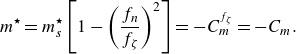 \begin{align} m^\star =m^\star _s\left [1-\left (\dfrac {f_n}{f_\zeta }\right )^2\right ]=-C^{\scriptscriptstyle f_\zeta }_m =-C_m. \end{align}
Without SRF, the condition $m^\star \gt 0$
implies that the added mass is negative, as also noted by Govardhan & Williamson (Reference Govardhan and Williamson2002). This means that only a part of the responses reached with SRF can be attained without SRF: the responses where the added mass is negative or, equivalently,
$m^\star \gt 0$
implies that the added mass is negative, as also noted by Govardhan & Williamson (Reference Govardhan and Williamson2002). This means that only a part of the responses reached with SRF can be attained without SRF: the responses where the added mass is negative or, equivalently, $f_\zeta \gt f_n$
. In the VIV regime, the oscillations are close to sinusoidal and (3.8) will be used to clarify the evolution of their properties when the conditions vary. The above analogy does not apply to the saccade regime, due to the irregular dynamics of the body.
$f_\zeta \gt f_n$
. In the VIV regime, the oscillations are close to sinusoidal and (3.8) will be used to clarify the evolution of their properties when the conditions vary. The above analogy does not apply to the saccade regime, due to the irregular dynamics of the body.
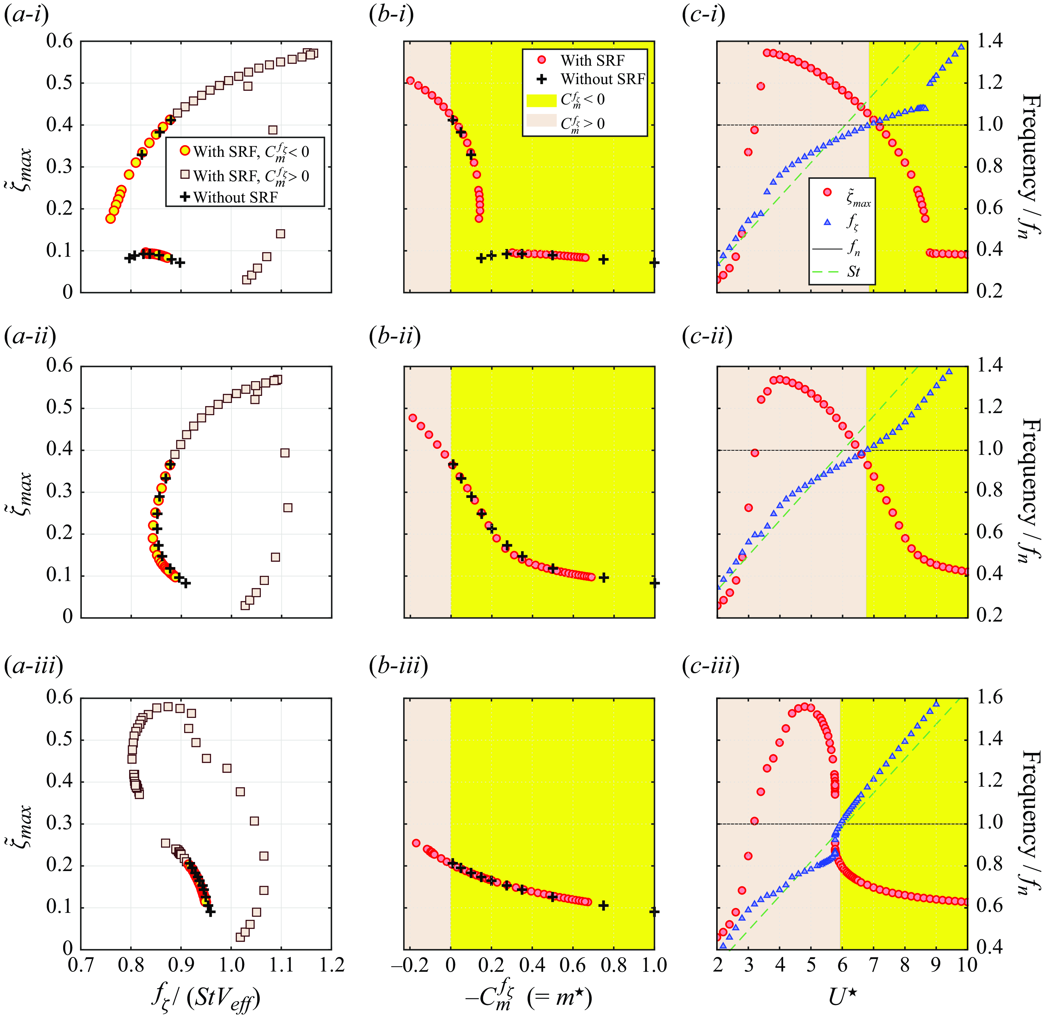
Figure 14. (a,b) Oscillation amplitude with and without SRF as a function of (a) the oscillation frequency and (b) $-C^{\scriptscriptstyle f_\zeta }_m$
. (c) Oscillation amplitude and frequency with SRF as functions of the reduced velocity. Three typical cases of the VIV regime are considered: (i)
$-C^{\scriptscriptstyle f_\zeta }_m$
. (c) Oscillation amplitude and frequency with SRF as functions of the reduced velocity. Three typical cases of the VIV regime are considered: (i) $(\theta ,{ Re},\alpha )=(90^\circ ,100,0)$
and
$(\theta ,{ Re},\alpha )=(90^\circ ,100,0)$
and $(\theta _{s},{ Re}_{s},\alpha _{s})=(90^\circ ,100,0)$
; (ii)
$(\theta _{s},{ Re}_{s},\alpha _{s})=(90^\circ ,100,0)$
; (ii) $(\theta ,{ Re},\alpha )=(90^\circ ,100,0.25)$
and
$(\theta ,{ Re},\alpha )=(90^\circ ,100,0.25)$
and $(\theta _{s},{ Re}_{s},\alpha _{s})=(69^\circ ,108,0.23)$
; (iii)
$(\theta _{s},{ Re}_{s},\alpha _{s})=(69^\circ ,108,0.23)$
; (iii) $(\theta ,{ Re},\alpha )=(90^\circ ,100,1)$
and
$(\theta ,{ Re},\alpha )=(90^\circ ,100,1)$
and $(\theta _{s},{ Re}_{s},\alpha _{s})=(41^\circ ,153,0.65)$
. With SRF, the mass ratio is set to
$(\theta _{s},{ Re}_{s},\alpha _{s})=(41^\circ ,153,0.65)$
. With SRF, the mass ratio is set to $1$
; without SRF,
$1$
; without SRF, $m^\star =-C^{\scriptscriptstyle f_\zeta }_m\in [0.01,1]$
. In (a), the oscillation frequency is normalised by the effective flow velocity magnitude and the Strouhal frequency; distinct symbols are used to designate the responses with SRF where
$m^\star =-C^{\scriptscriptstyle f_\zeta }_m\in [0.01,1]$
. In (a), the oscillation frequency is normalised by the effective flow velocity magnitude and the Strouhal frequency; distinct symbols are used to designate the responses with SRF where $C^{\scriptscriptstyle f_\zeta }_m$
is negative or positive, i.e. the responses accessible and inaccessible without SRF, respectively. In (b,c), yellow and grey background colours denote the regions where
$C^{\scriptscriptstyle f_\zeta }_m$
is negative or positive, i.e. the responses accessible and inaccessible without SRF, respectively. In (b,c), yellow and grey background colours denote the regions where $C^{\scriptscriptstyle f_\zeta }_m \lt 0$
and
$C^{\scriptscriptstyle f_\zeta }_m \lt 0$
and $C^{\scriptscriptstyle f_\zeta }_m \gt 0$
. In (c), the oscillation frequency is plotted together with the natural and Strouhal frequencies; the frequency range is normalised by the natural frequency.
$C^{\scriptscriptstyle f_\zeta }_m \gt 0$
. In (c), the oscillation frequency is plotted together with the natural and Strouhal frequencies; the frequency range is normalised by the natural frequency.
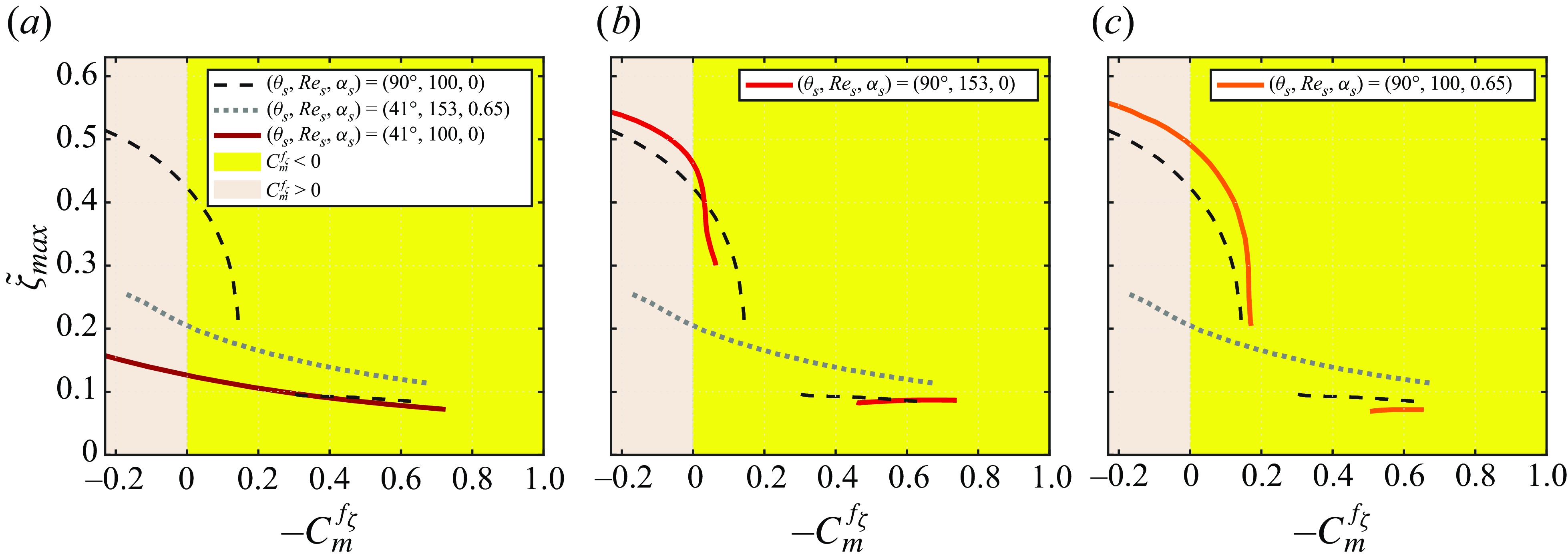
Figure 15. Oscillation amplitude with SRF as a function of $-C^{\scriptscriptstyle f_\zeta }_m$
for
$-C^{\scriptscriptstyle f_\zeta }_m$
for $(\theta _{s},{ Re}_{s},\alpha _{s})=(90^\circ ,100,0)$
and
$(\theta _{s},{ Re}_{s},\alpha _{s})=(90^\circ ,100,0)$
and $(\theta _{s},{ Re}_{s},\alpha _{s})=(41^\circ ,153,0.65)$
, which correspond to
$(\theta _{s},{ Re}_{s},\alpha _{s})=(41^\circ ,153,0.65)$
, which correspond to $(\theta ,{ Re},\alpha )=(90^\circ ,100,0)$
and
$(\theta ,{ Re},\alpha )=(90^\circ ,100,0)$
and $(\theta ,{ Re},\alpha )=(90^\circ ,100,1)$
without SRF. An additional case is considered in each panel to examine the specific influence of
$(\theta ,{ Re},\alpha )=(90^\circ ,100,1)$
without SRF. An additional case is considered in each panel to examine the specific influence of $\theta _{s}$
,
$\theta _{s}$
, ${ Re}_{s}$
and
${ Re}_{s}$
and $\alpha _{s}$
: (a)
$\alpha _{s}$
: (a) $(\theta _{s},{ Re}_{s},\alpha _{s})=(41^\circ ,100,0)$
; (b)
$(\theta _{s},{ Re}_{s},\alpha _{s})=(41^\circ ,100,0)$
; (b) $(\theta _{s},{ Re}_{s},\alpha _{s})=(90^\circ ,153,0)$
; (c)
$(\theta _{s},{ Re}_{s},\alpha _{s})=(90^\circ ,153,0)$
; (c) $(\theta _{s},{ Re}_{s},\alpha _{s})=(90^\circ ,100,0.65)$
. The mass ratio is set to
$(\theta _{s},{ Re}_{s},\alpha _{s})=(90^\circ ,100,0.65)$
. The mass ratio is set to $1$
. Yellow and grey background colours denote the regions of negative and positive added mass.
$1$
. Yellow and grey background colours denote the regions of negative and positive added mass.
As shown in § 3.2.1, the forced rotation attenuates the peak amplitudes of VIV. Here, this attenuation is discussed based on additional results issued from simulations of the system with SRF. With SRF, the body does not drift and the effective conditions match the nominal conditions. The conditions selected for the system with SRF correspond to the effective conditions of the system without SRF for $\theta =90^\circ$
, Re
$\theta =90^\circ$
, Re $\,=100$
and
$\,=100$
and $\alpha \in \{0,0.25,1\}$
. At fixed
$\alpha \in \{0,0.25,1\}$
. At fixed $(\theta ,{ Re},\alpha )$
, the effective conditions slightly vary with
$(\theta ,{ Re},\alpha )$
, the effective conditions slightly vary with $m^\star$
and the average values are considered in the simulations. To avoid confusion, as previously mentioned, the conditions of the system with SRF are denoted by the subscript
$m^\star$
and the average values are considered in the simulations. To avoid confusion, as previously mentioned, the conditions of the system with SRF are denoted by the subscript ${}_s$
. The mass ratio is set to
${}_s$
. The mass ratio is set to $1$
and the reduced velocity is varied to cover the bell-shaped curve of response amplitude. The oscillation amplitude measured with and without SRF for each case is plotted as a function of the oscillation frequency, normalised by the effective flow velocity magnitude and the Strouhal frequency, in figure 14(a), and as a function of the partial added mass coefficient, in figure 14(b). The partial added mass coefficient is referred to as the added mass coefficient in the following, to facilitate the reading. The conditions of the system with SRF are specified in the caption and located in the effective condition domain visited by the system without SRF in figure 5 (green stars). The responses reported in figure 14(a,b), with SRF for negative
$1$
and the reduced velocity is varied to cover the bell-shaped curve of response amplitude. The oscillation amplitude measured with and without SRF for each case is plotted as a function of the oscillation frequency, normalised by the effective flow velocity magnitude and the Strouhal frequency, in figure 14(a), and as a function of the partial added mass coefficient, in figure 14(b). The partial added mass coefficient is referred to as the added mass coefficient in the following, to facilitate the reading. The conditions of the system with SRF are specified in the caption and located in the effective condition domain visited by the system without SRF in figure 5 (green stars). The responses reported in figure 14(a,b), with SRF for negative $C^{\scriptscriptstyle f_\zeta }_m$
and without SRF, globally coincide. Slight differences can be noted due to the presence of small higher harmonic contributions, i.e. deviation from strictly sinusoidal evolutions, but the responses encountered with SRF provide a reasonable estimate of those arising without SRF.
$C^{\scriptscriptstyle f_\zeta }_m$
and without SRF, globally coincide. Slight differences can be noted due to the presence of small higher harmonic contributions, i.e. deviation from strictly sinusoidal evolutions, but the responses encountered with SRF provide a reasonable estimate of those arising without SRF.
The oscillation amplitude and frequency measured with SRF are represented as functions of the reduced velocity in figure 14(c). The conditions associated with an increase of $\alpha$
modify the shape of the response amplitude curve but do not diminish its peak values, as opposed to what was observed without SRF. The frequency range is normalised by
$\alpha$
modify the shape of the response amplitude curve but do not diminish its peak values, as opposed to what was observed without SRF. The frequency range is normalised by $f_n$
to delimit the responses accessible without SRF (
$f_n$
to delimit the responses accessible without SRF ( $C^{\scriptscriptstyle f_\zeta }_m\lt 0$
and
$C^{\scriptscriptstyle f_\zeta }_m\lt 0$
and $f_\zeta \gt f_n$
, based on (3.8)). The corresponding region is visualised by a yellow background colour while the inaccessible response region (
$f_\zeta \gt f_n$
, based on (3.8)). The corresponding region is visualised by a yellow background colour while the inaccessible response region ( $C^{\scriptscriptstyle f_\zeta }_m\gt 0$
and
$C^{\scriptscriptstyle f_\zeta }_m\gt 0$
and $f_\zeta \lt f_n$
) is indicated by a grey background colour. The oscillation frequency tends to follow the Strouhal frequency (green dashed line) and becomes larger than
$f_\zeta \lt f_n$
) is indicated by a grey background colour. The oscillation frequency tends to follow the Strouhal frequency (green dashed line) and becomes larger than $f_n$
for a reduced velocity close to
$f_n$
for a reduced velocity close to $6$
or
$6$
or $7$
, depending on the conditions. It can be noted that, under conditions emulating an increase of
$7$
, depending on the conditions. It can be noted that, under conditions emulating an increase of $\alpha$
, the amplitude range accessible without SRF is narrowed and restrained to substantially lower values than for
$\alpha$
, the amplitude range accessible without SRF is narrowed and restrained to substantially lower values than for $\alpha =0$
. Therefore, the rotation does not actually reduce the peak amplitudes, but shifts the large amplitudes towards the region of positive added mass, inaccessible without SRF.
$\alpha =0$
. Therefore, the rotation does not actually reduce the peak amplitudes, but shifts the large amplitudes towards the region of positive added mass, inaccessible without SRF.
When $\alpha$
is modified, the three parameters defining the effective conditions,
$\alpha$
is modified, the three parameters defining the effective conditions, $\theta _{{eff}}$
,
$\theta _{{eff}}$
, ${ Re}_{{eff}}$
and
${ Re}_{{eff}}$
and $\alpha _{{eff}}$
, vary simultaneously. This is also the case when
$\alpha _{{eff}}$
, vary simultaneously. This is also the case when $\theta$
or Re are modified, for a fixed value of
$\theta$
or Re are modified, for a fixed value of $\alpha \gt 0$
. The question that arises is whether the reduction of the range of large-amplitude oscillations accessible without SRF, and thus the amplitude attenuation noted for the present system, are governed by one of these parameters or by their combination. The specific influence of each parameter can be assessed individually for the system with SRF. In figure 15, the passage from the response amplitudes measured for
$\alpha \gt 0$
. The question that arises is whether the reduction of the range of large-amplitude oscillations accessible without SRF, and thus the amplitude attenuation noted for the present system, are governed by one of these parameters or by their combination. The specific influence of each parameter can be assessed individually for the system with SRF. In figure 15, the passage from the response amplitudes measured for $\alpha =0$
(figure 14
i) to those observed for
$\alpha =0$
(figure 14
i) to those observed for $\alpha =1$
(figure 14
iii) is examined by varying
$\alpha =1$
(figure 14
iii) is examined by varying $\theta _s$
in panel (a),
$\theta _s$
in panel (a), ${ Re}_s$
in panel (b) and
${ Re}_s$
in panel (b) and $\alpha _s$
in panel (c) (green dots in figure 5). It appears that the increase of
$\alpha _s$
in panel (c) (green dots in figure 5). It appears that the increase of ${ Re}_s$
or
${ Re}_s$
or $\alpha _s$
does not reduce the peak amplitude in the negative added mass region and, on the contrary, tends to increase it. In contrast, the reduction of
$\alpha _s$
does not reduce the peak amplitude in the negative added mass region and, on the contrary, tends to increase it. In contrast, the reduction of $\theta _s$
, from
$\theta _s$
, from $90^\circ$
to
$90^\circ$
to $41^\circ$
, considerably diminishes the peak amplitude. This effect of the incidence angle had been anticipated from prior results obtained with SRF in the absence of rotation (Bourguet Reference Bourguet2019), as mentioned in the introduction. Figure 15 suggests that, when
$41^\circ$
, considerably diminishes the peak amplitude. This effect of the incidence angle had been anticipated from prior results obtained with SRF in the absence of rotation (Bourguet Reference Bourguet2019), as mentioned in the introduction. Figure 15 suggests that, when $\alpha$
is increased, the attenuation of the peak amplitude is principally driven by the variation of the effective incidence angle, and not by the variation of the effective rotation rate or Reynolds number. This figure also indicates that the reduction the effective incidence angle leads to a smoother evolution of the amplitude (the amplitude jump vanishes from the negative added mass region), which is another effect of the rotation reported in § 3.2.1.
$\alpha$
is increased, the attenuation of the peak amplitude is principally driven by the variation of the effective incidence angle, and not by the variation of the effective rotation rate or Reynolds number. This figure also indicates that the reduction the effective incidence angle leads to a smoother evolution of the amplitude (the amplitude jump vanishes from the negative added mass region), which is another effect of the rotation reported in § 3.2.1.
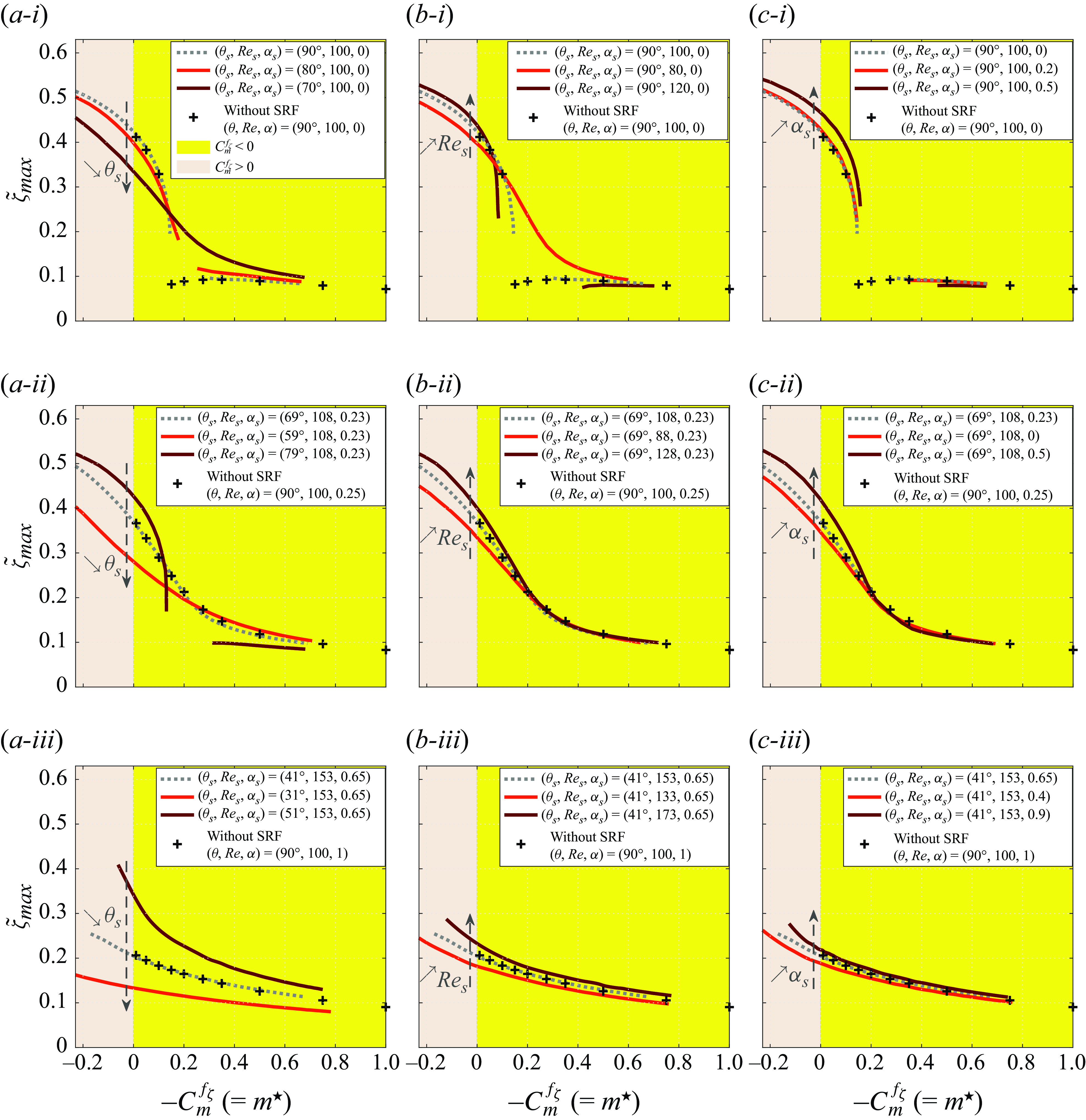
Figure 16. Oscillation amplitude with SRF as a function of $-C^{\scriptscriptstyle f_\zeta }_m$
for (i)
$-C^{\scriptscriptstyle f_\zeta }_m$
for (i) $(\theta _{s},{ Re}_{s},\alpha _{s})=(90^\circ ,100,0)$
, (ii)
$(\theta _{s},{ Re}_{s},\alpha _{s})=(90^\circ ,100,0)$
, (ii) $(\theta _{s},{ Re}_{s},\alpha _{s})=(69^\circ ,108,0.23)$
and (iii)
$(\theta _{s},{ Re}_{s},\alpha _{s})=(69^\circ ,108,0.23)$
and (iii) $(\theta _{s},{ Re}_{s},\alpha _{s})=(41^\circ ,153,0.65)$
, which correspond to
$(\theta _{s},{ Re}_{s},\alpha _{s})=(41^\circ ,153,0.65)$
, which correspond to $(\theta ,{ Re},\alpha )=(90^\circ ,100,0)$
,
$(\theta ,{ Re},\alpha )=(90^\circ ,100,0)$
, $(\theta ,{ Re},\alpha )=(90^\circ ,100,0.25)$
and
$(\theta ,{ Re},\alpha )=(90^\circ ,100,0.25)$
and $(\theta ,{ Re},\alpha )=(90^\circ ,100,1)$
without SRF; the amplitudes measured without SRF are also represented for comparison (symbols). Two additional cases with SRF, specified in the legend, are considered in each panel to examine the specific influence of
$(\theta ,{ Re},\alpha )=(90^\circ ,100,1)$
without SRF; the amplitudes measured without SRF are also represented for comparison (symbols). Two additional cases with SRF, specified in the legend, are considered in each panel to examine the specific influence of $\theta _{s}$
(a),
$\theta _{s}$
(a), ${ Re}_{s}$
(b) and
${ Re}_{s}$
(b) and $\alpha _{s}$
(c). The mass ratio is set to
$\alpha _{s}$
(c). The mass ratio is set to $1$
in the cases with SRF. Yellow and grey background colours denote the regions of negative and positive added mass. The trends identified by varying each parameter are indicated by dashed arrows.
$1$
in the cases with SRF. Yellow and grey background colours denote the regions of negative and positive added mass. The trends identified by varying each parameter are indicated by dashed arrows.
To confirm the trends identified in figure 15, the impact of a separate modulation of each parameter is visualised in figure 16, for the three cases considered in figure 14. The conditions covered by this sensitivity analysis are denoted by green diamonds in figure 5. In each panel of figure 16, a dashed arrow indicates the trend associated with a variation of the selected parameter in the region of negative added mass close to zero, i.e. the low- $m^\star$
range where the peak amplitudes are attained without SRF. These plots corroborate the above observations, in particular, the diminution of the peak amplitudes as
$m^\star$
range where the peak amplitudes are attained without SRF. These plots corroborate the above observations, in particular, the diminution of the peak amplitudes as $\theta _s$
is reduced. Focus is placed here on a variation of
$\theta _s$
is reduced. Focus is placed here on a variation of $\alpha$
, where the alterations of the three effective conditions have opposite influences on the oscillation amplitude. This is also the case when
$\alpha$
, where the alterations of the three effective conditions have opposite influences on the oscillation amplitude. This is also the case when $\theta$
is varied at fixed
$\theta$
is varied at fixed $\alpha \gt 0$
. A reduction of
$\alpha \gt 0$
. A reduction of $\theta$
causes an increase of
$\theta$
causes an increase of $\alpha _{{eff}}$
, which is expected to amplify the oscillation (based on figure 16), but reductions of
$\alpha _{{eff}}$
, which is expected to amplify the oscillation (based on figure 16), but reductions of ${ Re}_{{eff}}$
and
${ Re}_{{eff}}$
and $\theta _{{eff}}$
, which are expected to attenuate it. The peak amplitudes are actually attenuated (figure 6
a).
$\theta _{{eff}}$
, which are expected to attenuate it. The peak amplitudes are actually attenuated (figure 6
a).
The analysis of the impact of the rotation in the VIV regime can be recapitulated as follows. Through the accessible/inaccessible response prism, the rotation is found to enhance the divergence between the behaviours of the systems with and without SRF: as $\alpha$
is increased, most of the large-amplitude oscillations tend to be associated with positive added mass and thus become inaccessible without SRF, which results in a reduction of the peak amplitudes in this case. A variation of the rotation rate induces a modification of all the effective conditions. Yet, VIV attenuation appears to be essentially governed by the alteration of a single condition, the effective incidence angle. This analysis closes the exploration of the physical mechanisms involved in the different regimes of the flow–body system. The principal findings of the present work are summarised hereafter.
$\alpha$
is increased, most of the large-amplitude oscillations tend to be associated with positive added mass and thus become inaccessible without SRF, which results in a reduction of the peak amplitudes in this case. A variation of the rotation rate induces a modification of all the effective conditions. Yet, VIV attenuation appears to be essentially governed by the alteration of a single condition, the effective incidence angle. This analysis closes the exploration of the physical mechanisms involved in the different regimes of the flow–body system. The principal findings of the present work are summarised hereafter.
4. Conclusions
The behaviour of the system composed of a circular cylinder, free to translate along a rectilinear path in an arbitrary direction under the effect of a cross-current and forced to rotate about its axis, has been investigated numerically, at a Reynolds number equal to $100$
. This work represents an extension of prior studies concerning the transverse flow-induced vibrations of a non-rotating cylinder without structural restoring force. The impact of the rectilinear path orientation, which was varied from the transverse (
$100$
. This work represents an extension of prior studies concerning the transverse flow-induced vibrations of a non-rotating cylinder without structural restoring force. The impact of the rectilinear path orientation, which was varied from the transverse ( $\theta =90^\circ$
) to the streamwise (
$\theta =90^\circ$
) to the streamwise ( $\theta =0^\circ$
) direction, and the influence of the rotation rate (
$\theta =0^\circ$
) direction, and the influence of the rotation rate ( $\alpha \in [0,1]$
) were explored over a range of low mass ratios,
$\alpha \in [0,1]$
) were explored over a range of low mass ratios, $m^\star \in [0.01,1]$
.
$m^\star \in [0.01,1]$
.
The cylinder displacement can be decomposed into a linear term, which governs the drift of the body and depends on its time-averaged velocity, i.e. the drift velocity, and a fluctuation of bounded magnitude. The drift velocity is only marginally altered by body oscillation/flow unsteadiness and variations of $m^\star$
. It can be predicted via a quasi-steady model of the tangential force. The effective conditions associated with the flow seen by the drifting body substantially vary across the
$m^\star$
. It can be predicted via a quasi-steady model of the tangential force. The effective conditions associated with the flow seen by the drifting body substantially vary across the $(\theta ,\alpha )$
domain and differ from the nominal conditions based on the oncoming flow. In particular, they include the critical threshold of flow unsteadiness for a rigidly mounted cylinder. The rotation may considerably amplify the effective flow, leading to effective Reynolds numbers close to
$(\theta ,\alpha )$
domain and differ from the nominal conditions based on the oncoming flow. In particular, they include the critical threshold of flow unsteadiness for a rigidly mounted cylinder. The rotation may considerably amplify the effective flow, leading to effective Reynolds numbers close to $160$
. It also disrupts the phenomenon of symmetry recovery observed for
$160$
. It also disrupts the phenomenon of symmetry recovery observed for $\alpha =0$
(
$\alpha =0$
( $\theta _{{eff}}=90^\circ$
regardless of
$\theta _{{eff}}=90^\circ$
regardless of $\theta \ne 0^\circ$
) and introduces a dependence of the effective incidence angle on
$\theta \ne 0^\circ$
) and introduces a dependence of the effective incidence angle on $\theta$
.
$\theta$
.
Three distinct regimes of the flow–body system have been identified within the parameter space under study. Their principal properties can be summarised as follows.
Pure drift regime. In this regime, which occurs in subcritical effective conditions, below an incidence angle ranging from $\theta \approx 7^\circ$
to
$\theta \approx 7^\circ$
to $\theta \approx 23^\circ$
depending on
$\theta \approx 23^\circ$
depending on $m^\star$
and
$m^\star$
and $\alpha$
, the cylinder translates at a constant velocity, without fluctuation of its displacement. The instantaneous flow seen by the body is steady. The rotation causes an asymmetry in the shapes and magnitudes of the elongated positive and negative vorticity layers composing the wake of the drifting cylinder.
$\alpha$
, the cylinder translates at a constant velocity, without fluctuation of its displacement. The instantaneous flow seen by the body is steady. The rotation causes an asymmetry in the shapes and magnitudes of the elongated positive and negative vorticity layers composing the wake of the drifting cylinder.
VIV regime. The vortex-induced vibrations reported in previous works concerning a cylinder without SRF, for $\theta = 90^\circ$
and
$\theta = 90^\circ$
and $\alpha =0$
, are found to persist as
$\alpha =0$
, are found to persist as $\theta$
is reduced down to the frontier of the pure drift regime, over the entire
$\theta$
is reduced down to the frontier of the pure drift regime, over the entire $\alpha$
range. This includes a region of subcritical effective conditions. In the VIV regime, the oscillation of the body is periodic, nearly sinusoidal, and synchronised with flow unsteadiness. The oscillation frequency is close to the Strouhal frequency and the organisation of the flow resembles the von Kármán street developing downstream of a fixed cylinder, with the shedding of a pair of counter-rotating spanwise vortices per cycle. The peak amplitude of oscillation, close to
$\alpha$
range. This includes a region of subcritical effective conditions. In the VIV regime, the oscillation of the body is periodic, nearly sinusoidal, and synchronised with flow unsteadiness. The oscillation frequency is close to the Strouhal frequency and the organisation of the flow resembles the von Kármán street developing downstream of a fixed cylinder, with the shedding of a pair of counter-rotating spanwise vortices per cycle. The peak amplitude of oscillation, close to $0.4D$
, is attained at normal incidence without rotation, for the lowest mass ratio. The rotation breaks the transverse symmetry of the system dynamics relative to the effective flow and slightly perturbs the antisymmetrical pattern of the wake. The flow past the oscillating body becomes three-dimensional at high incidence angles for
$0.4D$
, is attained at normal incidence without rotation, for the lowest mass ratio. The rotation breaks the transverse symmetry of the system dynamics relative to the effective flow and slightly perturbs the antisymmetrical pattern of the wake. The flow past the oscillating body becomes three-dimensional at high incidence angles for $\alpha \gt 0.4$
. It remains however structured by the two-dimensional vortex shedding and its three-dimensionality has only a limited influence on fluid forcing and body response. The most salient effect of the rotation is a homogenisation of VIV amplitude/frequency in the
$\alpha \gt 0.4$
. It remains however structured by the two-dimensional vortex shedding and its three-dimensionality has only a limited influence on fluid forcing and body response. The most salient effect of the rotation is a homogenisation of VIV amplitude/frequency in the $(\theta ,m^\star )$
domain, with a notable attenuation of the peak amplitude oscillations in the lower-
$(\theta ,m^\star )$
domain, with a notable attenuation of the peak amplitude oscillations in the lower- $m^\star$
range; the maximum amplitude is divided by
$m^\star$
range; the maximum amplitude is divided by $2$
for
$2$
for $\alpha =1$
. This attenuation has been analysed in light of the behavior of the system with SRF, and it appears to be mainly driven by the reduction of the effective incidence angle that accompanies the alteration of the drift velocity, as
$\alpha =1$
. This attenuation has been analysed in light of the behavior of the system with SRF, and it appears to be mainly driven by the reduction of the effective incidence angle that accompanies the alteration of the drift velocity, as $\alpha$
is increased.
$\alpha$
is increased.
Saccade regime. A second oscillatory regime, triggered by the rotation, was uncovered close to $\theta =0^\circ$
, where the drift velocity matches the oncoming flow velocity and the effective flow vanishes. The effective configuration essentially corresponds to the problem of a rotating cylinder placed in quiescent fluid. In this regime, the displacement of the body about its drifting motion is aperiodic and consists of irregular jumps of variable amplitudes. These jumps were called saccades to emphasise the jerky character of the dynamics, compared with the regularity of VIV. Saccades typically reach
$\theta =0^\circ$
, where the drift velocity matches the oncoming flow velocity and the effective flow vanishes. The effective configuration essentially corresponds to the problem of a rotating cylinder placed in quiescent fluid. In this regime, the displacement of the body about its drifting motion is aperiodic and consists of irregular jumps of variable amplitudes. These jumps were called saccades to emphasise the jerky character of the dynamics, compared with the regularity of VIV. Saccades typically reach $10$
body diameters and their frequencies are one or more orders of magnitude lower than VIV frequencies. The structural response is insensitive to the value of the mass ratio. The interaction of the cylinder with the vorticity layers wrapped around it appears to play a central role in the emergence of this regime. The importance of flow unsteadiness is further substantiated by the fact that the saccades are not captured by a quasi-steady modelling of fluid forcing. An increase of
$10$
body diameters and their frequencies are one or more orders of magnitude lower than VIV frequencies. The structural response is insensitive to the value of the mass ratio. The interaction of the cylinder with the vorticity layers wrapped around it appears to play a central role in the emergence of this regime. The importance of flow unsteadiness is further substantiated by the fact that the saccades are not captured by a quasi-steady modelling of fluid forcing. An increase of $\alpha$
tends to reduce the oscillation amplitude, as in the VIV regime, but enhances the erratic nature of the system behaviour.
$\alpha$
tends to reduce the oscillation amplitude, as in the VIV regime, but enhances the erratic nature of the system behaviour.
Funding
This work was performed using HPC resources from CALMIP (grant 2024-P1248).
Declaration of interests
The author reports no conflict of interest.
Appendix. Implications of system symmetry
For the present system, the incidence angles $\theta$
and
$\theta$
and $\theta +180^\circ$
correspond to the same physical configuration and the range
$\theta +180^\circ$
correspond to the same physical configuration and the range $\theta \in [0^\circ ,180^\circ ]$
is considered here. Additional connections can be established between the system behaviours at different incidence angles, as shown in this Appendix. The velocity of the instantaneous flow seen by the body moving at incidence
$\theta \in [0^\circ ,180^\circ ]$
is considered here. Additional connections can be established between the system behaviours at different incidence angles, as shown in this Appendix. The velocity of the instantaneous flow seen by the body moving at incidence $\theta$
and velocity
$\theta$
and velocity $\dot \zeta$
, visualised in red colour in figure 17, is equal to
$\dot \zeta$
, visualised in red colour in figure 17, is equal to $\{1-{\dot \zeta }\cos (\theta ),-{\dot \zeta }\sin (\theta ),0\}^{\textrm { T}}$
, in the
$\{1-{\dot \zeta }\cos (\theta ),-{\dot \zeta }\sin (\theta ),0\}^{\textrm { T}}$
, in the $(x,y,z)$
frame. Its magnitude and the relative incidence of body trajectory with respect to this velocity can be expressed respectively as follows:
$(x,y,z)$
frame. Its magnitude and the relative incidence of body trajectory with respect to this velocity can be expressed respectively as follows:
 \begin{align} V_{{ ins}}=\sqrt {\dot \zeta ^2-2\dot \zeta \cos \left (\theta \right )+1} \,\,\,\textrm { and}\quad \theta _{{ ins}}=\arctan \left (\dfrac {\sin \left (\theta \right )}{\cos \left (\theta \right )-\dot \zeta }\right ). \end{align}
The subscript ${}_{{ ins}}$
is used in reference to the instantaneous flow. In a second configuration denoted by
${}_{{ ins}}$
is used in reference to the instantaneous flow. In a second configuration denoted by ${}'$
, for
${}'$
, for $\theta$
and
$\theta$
and $\theta '$
in
$\theta '$
in $]0^\circ ,180^\circ [$
, if the oncoming flow velocity magnitude and body velocity satisfy
$]0^\circ ,180^\circ [$
, if the oncoming flow velocity magnitude and body velocity satisfy
 \begin{align} \dfrac {U'}{U}=\dfrac {\sin \left (\theta \right )}{\sin \left (\theta '\right )}\,\,\,\textrm { and}\quad \dot \zeta '=\dfrac {\sin \left (\theta '\right )}{\sin \left (\theta \right )}\left (\dot \zeta -\cos \left (\theta \right )\right )+\cos \left (\theta '\right ), \end{align}
then $V'_{{ ins}}U'=V_{{ ins}}U$
and
$V'_{{ ins}}U'=V_{{ ins}}U$
and $\theta '_{{ ins}}=\theta _{{ ins}}$
, which means that the instantaneous flow seen by the body is the same as in the first configuration, and so is the tangential force,
$\theta '_{{ ins}}=\theta _{{ ins}}$
, which means that the instantaneous flow seen by the body is the same as in the first configuration, and so is the tangential force, $C'U'^2=CU^2$
.
$C'U'^2=CU^2$
.
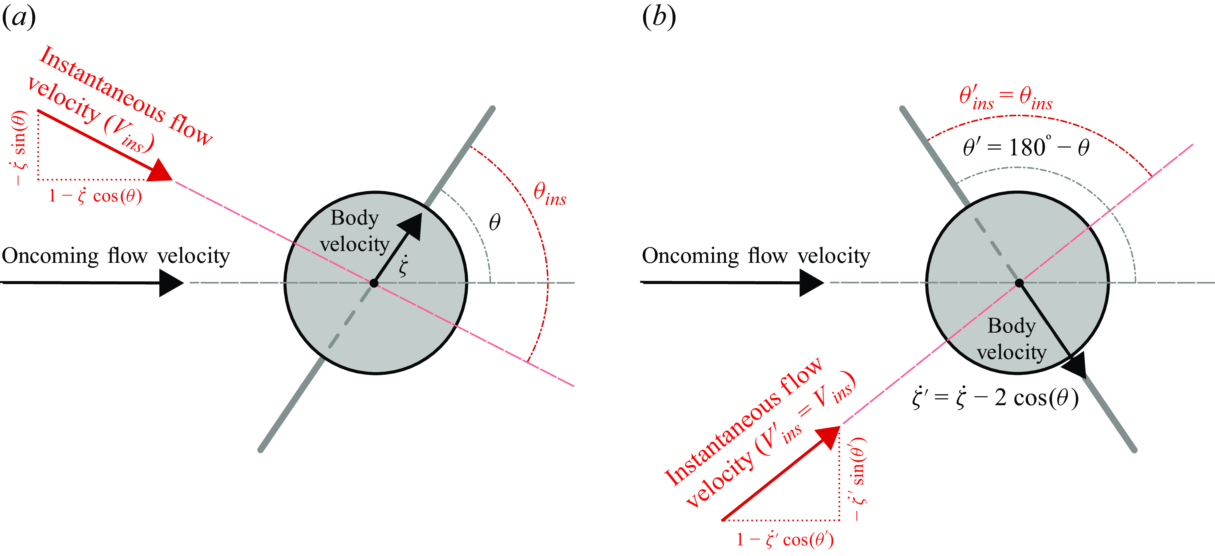
Figure 17. Sketch of the instantaneous flow seen by the cylinder moving at (a) incidence $\theta$
and velocity
$\theta$
and velocity $\dot \zeta$
, and (b) incidence
$\dot \zeta$
, and (b) incidence $\theta '=180^\circ -\theta$
and velocity
$\theta '=180^\circ -\theta$
and velocity $\dot \zeta '=\dot \zeta -2\cos (\theta )$
. The instantaneous flow (visualised in red colour) is the same in both cases, i.e. same velocity magnitude (
$\dot \zeta '=\dot \zeta -2\cos (\theta )$
. The instantaneous flow (visualised in red colour) is the same in both cases, i.e. same velocity magnitude ( $V_{{ ins}}$
) and same relative incidence of body trajectory (
$V_{{ ins}}$
) and same relative incidence of body trajectory ( $\theta _{{ ins}}$
).
$\theta _{{ ins}}$
).
In the particular case, depicted in figure 17, where $\theta '=180^\circ -\theta$
, the relations (A2) become
$\theta '=180^\circ -\theta$
, the relations (A2) become $U'=U$
and
$U'=U$
and $\dot \zeta '=\dot \zeta -2\cos (\theta )$
. If the structural dynamics
$\dot \zeta '=\dot \zeta -2\cos (\theta )$
. If the structural dynamics $(\ddot \zeta ,\dot \zeta ,\zeta )$
is a solution of (2.2) at incidence
$(\ddot \zeta ,\dot \zeta ,\zeta )$
is a solution of (2.2) at incidence $\theta$
, then
$\theta$
, then $(\ddot \zeta ',\dot \zeta ',\zeta ')=(\ddot \zeta ,\dot \zeta -2\cos (\theta ),\zeta -2\cos (\theta )t)$
is a solution of this equation at incidence
$(\ddot \zeta ',\dot \zeta ',\zeta ')=(\ddot \zeta ,\dot \zeta -2\cos (\theta ),\zeta -2\cos (\theta )t)$
is a solution of this equation at incidence $180^\circ -\theta$
;
$180^\circ -\theta$
; $t$
designates the non-dimensional time variable. Therefore, the solutions of (2.2) for
$t$
designates the non-dimensional time variable. Therefore, the solutions of (2.2) for $\theta \in [90^\circ ,180^\circ ]$
can be deduced from those obtained for
$\theta \in [90^\circ ,180^\circ ]$
can be deduced from those obtained for $\theta \in [0^\circ ,90^\circ ]$
, at the same
$\theta \in [0^\circ ,90^\circ ]$
, at the same $m^\star$
, Re and
$m^\star$
, Re and $\alpha$
. The fluctuation of the displacement about its linear trend,
$\alpha$
. The fluctuation of the displacement about its linear trend, $\tilde \zeta =\zeta -\overline {\dot \zeta }t$
, where
$\tilde \zeta =\zeta -\overline {\dot \zeta }t$
, where $\overline {\phantom {a}}$
denotes the time-averaged value, is the same in both configurations,
$\overline {\phantom {a}}$
denotes the time-averaged value, is the same in both configurations, $\tilde \zeta '=\tilde \zeta$
. The behaviour of the system in terms of flow dynamics, fluid forcing and body displacement fluctuation is thus symmetrical about
$\tilde \zeta '=\tilde \zeta$
. The behaviour of the system in terms of flow dynamics, fluid forcing and body displacement fluctuation is thus symmetrical about $\theta =90^\circ$
. In the paper, the results are presented for
$\theta =90^\circ$
. In the paper, the results are presented for $\theta \in [0^\circ ,90^\circ ]$
.
$\theta \in [0^\circ ,90^\circ ]$
.


 Open access