


1. Introduction
1.1. Electrodynamic particulate suspension
Electrodynamic particulate suspension (EPS) is a method of generating suspensions of electrically conducting particles using electric forces instead of hydrodynamic forces to lift the particles (Colver Reference Colver1980; Yu & Colver Reference Yu and Colver1987; Colver & Ehlinger Reference Colver and Ehlinger1988; Shoshin & Dreizin Reference Shoshin and Dreizin2002). In the simplest case, a suspension of high electrical conductivity particles is formed in the gap between two horizontal electrodes set at different electric potentials. The particles in contact with the lower electrode are instantly charged to the potential of this electrode, and experience a vertical force that may detach them from the electrode and push them upwards across the gap. When these particles hit the upper electrode, they get charged to this electrode potential, which reverses the polarity of their charge and the direction of the electric force, so they fall until they hit the lower electrode and the cycle repeats.
Numerical simulations of dilute suspensions of monodisperse particles of high electrical conductivity with negligible inertia were carried out by Zhebelev (Reference Zhebelev1992) taking into account the collisions between the particles and the electric field induced by their charges. This author proposed the so-called field mechanism, according to which the maximum number of particles that can be suspended per unit electrode area for a given interelectrode voltage is determined by the condition that the space charge induced field reduces the net field at the lower electrode to the minimum value required for the electric force to balance the weight of the particles. A different, recombination mechanism, limiting the number of suspended particles to a value independent of the voltage, was proposed by Bologa, Grosu & Kozhukhar (Reference Bologa, Grosu and Kozhukhar1977), Myazdrikov (Reference Myazdrikov1984) and Zhebelev (Reference Zhebelev1992), while Zhebelev (Reference Zhebelev1991, Reference Zhebelev1993) and Higuera (Reference Higuera2023) carried out simulations for suspensions of finite conductivity particles, for which the electric relaxation time is not small compared with the contact time in collisions with the electrodes or among particles.
In applications, a spray is generated by blowing a gas through the suspension. This allows controlling the spray velocity independently of the spray density, which is controlled by the voltage between the electrodes. The existence of two control parameters makes for a flexible technique, which has been used for surface treatments, deposition of coatings and catalytic layers, powder metallurgy (Myazdrikov Reference Myazdrikov1980), and powder spray combustion (Bologa, Solomyanchuk & Berkov 1988; Kim Reference Kim1989; Colver, Kim & Yu Reference Colver, Kim and Yu1996; Shoshin & Dreizin Reference Shoshin and Dreizin2002, Reference Shoshin and Dreizin2003, Reference Shoshin and Dreizin2004, Reference Shoshin and Dreizin2006; Colver et al. Reference Colver, Greene, Shoemaker and Yu2004). Other applications include acceleration of iron microparticles for impact studies (Shelton, Hendricks & Wuerker Reference Shelton, Hendricks and Wuerker1960), beneficiation of iron ores and other fines (Inculet, Bergougnou & Bauer Reference Inculet, Bergougnoe and Bauer1972; Kiewiet et al. 1978), dust cleaning (Melcher & Sachar Reference Melcher and Sachar1974), trapping of particulate contaminants in high voltage systems (Cooke Reference Cooke1980), and enhanced heat transfer (Dietz & Melcher Reference Dietz and Melcher1975; Bologa, Pushkov & Berkov 1985; Estami & Esmaelzadeh Reference Estami and Esmaelzadeh2017).
Despite its long history, EPS abounds with complex issues that are not fully understood. Among the important questions that will not be addressed in this work are: (i) adhesion forces, which play an important part in particle/electrode interactions and may increase the interelectrode voltage required to first suspend particles to values well above those needed to keep an already established suspension; (ii) effects of finite bulk and surface electrical conductivity of the particles, which may be difficult to estimate in cases when transfer of charge across a layer of oxide on the surface of the particles is involved, and introduce electrical relaxation times into the problem; (iii) inelastic effects in particle collisions; (iv) electric discharges in the gas surrounding the particles; and (v) electric forces on deposited particles in the presence of other nearby particles.
1.2. Scope of this work
We consider a dilute suspension of solid spherical particles of mass $m$
, radius
$m$
, radius $a$
, and high electrical conductivity in a gas. The electric charge of each particle is conserved in its drift and is instantly redistributed in particle collisions. Only binary collisions are relevant for dilute suspensions, with a number density of particles
$a$
, and high electrical conductivity in a gas. The electric charge of each particle is conserved in its drift and is instantly redistributed in particle collisions. Only binary collisions are relevant for dilute suspensions, with a number density of particles $n$
satisfying
$n$
satisfying $n a^3 \ll 1$
. The volume fraction of the particles is assumed to be very small.
$n a^3 \ll 1$
. The volume fraction of the particles is assumed to be very small.
Let $q_1$
and
$q_1$
and $q_2$
be the charges of two colliding particles. If the collision occurs at a point where the electric field induced by an externally applied voltage and the charges of other suspension particles is
$q_2$
be the charges of two colliding particles. If the collision occurs at a point where the electric field induced by an externally applied voltage and the charges of other suspension particles is $\boldsymbol{E}$
, then the particles emerge from the collision with charges
$\boldsymbol{E}$
, then the particles emerge from the collision with charges $(q_1+q_2)/2 \pm q_{_E}$
, with
$(q_1+q_2)/2 \pm q_{_E}$
, with $q_{_E}=\gamma \epsilon _0 a^2 E_{lc}$
. Here,
$q_{_E}=\gamma \epsilon _0 a^2 E_{lc}$
. Here, $\gamma =2 \unicode{x03C0} ( {8 \ln 2 - \unicode{x03C0} ^2/3} ) \approx 14.17$
(Ling & Higuera Reference Ling and Higuera2022),
$\gamma =2 \unicode{x03C0} ( {8 \ln 2 - \unicode{x03C0} ^2/3} ) \approx 14.17$
(Ling & Higuera Reference Ling and Higuera2022), $\epsilon _{0}$
is the electrical permittivity of the gas surrounding the particles, and
$\epsilon _{0}$
is the electrical permittivity of the gas surrounding the particles, and $E_{lc}$
is the component of
$E_{lc}$
is the component of $\boldsymbol{E}$
in the direction of the line joining the centres of the colliding particles. The upper sign is for the particle facing the field, which acquires the excess of charge
$\boldsymbol{E}$
in the direction of the line joining the centres of the colliding particles. The upper sign is for the particle facing the field, which acquires the excess of charge $q_{_E}$
above the average value
$q_{_E}$
above the average value $(q_1+q_2)/2$
, and the lower sign is for the rearing particle, which emerges with an equal defect of charge.
$(q_1+q_2)/2$
, and the lower sign is for the rearing particle, which emerges with an equal defect of charge.
The momentum and the kinetic energy of the particles are assumed to be conserved in the collisions, leaving out dissipation due to mechanical friction or inelastic effects. Calling $q_c$
the characteristic charge of a particle, the order of the electric force between two particles spaced at a distance of order
$q_c$
the characteristic charge of a particle, the order of the electric force between two particles spaced at a distance of order $a$
is
$a$
is $q_c^2/ ( {4 \unicode{x03C0} \epsilon _0 a^2} )$
(larger than this by a logarithmic factor when the distance between the particle surfaces is small compared with
$q_c^2/ ( {4 \unicode{x03C0} \epsilon _0 a^2} )$
(larger than this by a logarithmic factor when the distance between the particle surfaces is small compared with $a$
; see Lekner Reference Lekner2011), while the force that the electric field due to the applied voltage and the charge of the whole suspension (of order
$a$
; see Lekner Reference Lekner2011), while the force that the electric field due to the applied voltage and the charge of the whole suspension (of order $E_c$
say) exerts on a particle is of order
$E_c$
say) exerts on a particle is of order $q_c E_c$
. The two forces are of the same order if
$q_c E_c$
. The two forces are of the same order if $q_c=\gamma \epsilon _0 a^2 E_c$
(see below). However, the first force rapidly decreases when the distance between the colliding particles becomes large compared with
$q_c=\gamma \epsilon _0 a^2 E_c$
(see below). However, the first force rapidly decreases when the distance between the colliding particles becomes large compared with $a$
(in a time of order
$a$
(in a time of order $a/v_c$
, where
$a/v_c$
, where $v_c$
is the typical velocity of the particles), while the second force persists longer and leads to particle velocities
$v_c$
is the typical velocity of the particles), while the second force persists longer and leads to particle velocities $v_c=q_c E_c t_{acc}/m$
, where
$v_c=q_c E_c t_{acc}/m$
, where $t_{acc}$
is the smaller of the time between particle collisions
$t_{acc}$
is the smaller of the time between particle collisions $t_{coll}$
(the inverse of the collision frequency) and the viscous adaptation time
$t_{coll}$
(the inverse of the collision frequency) and the viscous adaptation time $t_s=m/c_f$
. Here, the Reynolds number of the flow of the gas around the particle is assumed to be small, so the friction coefficient is
$t_s=m/c_f$
. Here, the Reynolds number of the flow of the gas around the particle is assumed to be small, so the friction coefficient is $c_f=6 \unicode{x03C0} \mu _g a$
, with
$c_f=6 \unicode{x03C0} \mu _g a$
, with $\mu _g$
the viscosity of the gas. Thus in first approximation, the charges of the particles play no role in the redistribution of momentum and kinetic energy in the collisions, which are as for the collisions in a gas of neutral rigid spheres.
$\mu _g$
the viscosity of the gas. Thus in first approximation, the charges of the particles play no role in the redistribution of momentum and kinetic energy in the collisions, which are as for the collisions in a gas of neutral rigid spheres.
Two limiting cases may be considered, depending on the value of the ratio $t_{coll}/t_s$
of the mean time between collisions to the viscous adaptation time. If this ratio is large, then viscous friction with the gas rapidly changes the velocity of a particle emerging from a collision with charge
$t_{coll}/t_s$
of the mean time between collisions to the viscous adaptation time. If this ratio is large, then viscous friction with the gas rapidly changes the velocity of a particle emerging from a collision with charge $q$
. The particle reaches the terminal velocity
$q$
. The particle reaches the terminal velocity ${\boldsymbol{v}}={\boldsymbol{v}}_g + (q {\boldsymbol{E}} + m {\boldsymbol{g}})/c_f$
, with
${\boldsymbol{v}}={\boldsymbol{v}}_g + (q {\boldsymbol{E}} + m {\boldsymbol{g}})/c_f$
, with ${\boldsymbol{v}}_g$
the velocity of the gas, and
${\boldsymbol{v}}_g$
the velocity of the gas, and $\boldsymbol{g}$
the acceleration of gravity, in a time of order
$\boldsymbol{g}$
the acceleration of gravity, in a time of order $t_s$
, and the effect of the particle inertia is negligible in the rest of the particle streaming. This short viscous adaptation stage can be considered part of the collision, which then conserves the number and charge of the particles but does not conserve momentum and energy. Taking this view, the trajectories of the particles consist of streaming periods in which the particles move at the terminal velocity corresponding to the local instantaneous values of
$t_s$
, and the effect of the particle inertia is negligible in the rest of the particle streaming. This short viscous adaptation stage can be considered part of the collision, which then conserves the number and charge of the particles but does not conserve momentum and energy. Taking this view, the trajectories of the particles consist of streaming periods in which the particles move at the terminal velocity corresponding to the local instantaneous values of ${\boldsymbol{v}}_g$
and
${\boldsymbol{v}}_g$
and $\boldsymbol{E}$
, punctuated by nearly instantaneous binary collisions that redistribute the charges of the colliding particles and leave them moving with the terminal velocities corresponding to their new charges. The system can be described using a reduced distribution function of the form
$\boldsymbol{E}$
, punctuated by nearly instantaneous binary collisions that redistribute the charges of the colliding particles and leave them moving with the terminal velocities corresponding to their new charges. The system can be described using a reduced distribution function of the form $F(q, E, {\boldsymbol{x}}, t)$
, where the dependence on
$F(q, E, {\boldsymbol{x}}, t)$
, where the dependence on $E$
is brought in by
$E$
is brought in by $q_{_E}$
.
$q_{_E}$
.
This viscosity-dominated regime has been discussed elsewhere, e.g. Higuera (Reference Higuera2018) and Ling & Higuera (Reference Ling and Higuera2022). The first of these papers introduced a kinetic equation for the distribution function $F$
(see (2.1) below), and the second computed the equilibrium distribution function in the continuum regime when the mean free path between particles collisions,
$F$
(see (2.1) below), and the second computed the equilibrium distribution function in the continuum regime when the mean free path between particles collisions, $\lambda \sim 1/(n_c a^2)$
with
$\lambda \sim 1/(n_c a^2)$
with $n_c$
the typical number of particles per unit volume, is small compared with the characteristic size of the suspension, denoted by
$n_c$
the typical number of particles per unit volume, is small compared with the characteristic size of the suspension, denoted by $L$
in what follows. This regime will be revisited in § 2 to: (i) establish a connection between the continuum regime and quasi-neutrality of the suspension, and (ii) investigate the non-uniform manner in which the continuum regime is approached for high voltages and high values of the number of suspended particles per unit electrode area in an EPS cell.
$L$
in what follows. This regime will be revisited in § 2 to: (i) establish a connection between the continuum regime and quasi-neutrality of the suspension, and (ii) investigate the non-uniform manner in which the continuum regime is approached for high voltages and high values of the number of suspended particles per unit electrode area in an EPS cell.
In the opposite case when $t_{coll}/t_s$
is small, the effect of the particle inertia must be accounted for in streaming between collisions. The description of the suspension must rely on a full distribution function
$t_{coll}/t_s$
is small, the effect of the particle inertia must be accounted for in streaming between collisions. The description of the suspension must rely on a full distribution function $f({\boldsymbol{v}}, q, E, {\boldsymbol{x}}, t)$
, which gives the mean number of particles moving with velocities in the range between
$f({\boldsymbol{v}}, q, E, {\boldsymbol{x}}, t)$
, which gives the mean number of particles moving with velocities in the range between $\boldsymbol{v}$
and
$\boldsymbol{v}$
and ${\boldsymbol{v}} + \textrm {d} {\boldsymbol{v}}$
, and bearing charges between
${\boldsymbol{v}} + \textrm {d} {\boldsymbol{v}}$
, and bearing charges between $q$
and
$q$
and $q + \textrm {d} q$
per unit volume, about a point
$q + \textrm {d} q$
per unit volume, about a point $\boldsymbol{x}$
at a time
$\boldsymbol{x}$
at a time $t$
as
$t$
as $f({\boldsymbol{v}}, q, E, {\boldsymbol{x}}, t) \, \textrm {d} {\boldsymbol{v}} \, \textrm {d} q$
. This distribution function obeys a Boltzmann equation. However, the redistribution of charge in collisions described above has an irreversible contractive character (more evident if
$f({\boldsymbol{v}}, q, E, {\boldsymbol{x}}, t) \, \textrm {d} {\boldsymbol{v}} \, \textrm {d} q$
. This distribution function obeys a Boltzmann equation. However, the redistribution of charge in collisions described above has an irreversible contractive character (more evident if $q_{_E}$
is left out) that invalidates the principle of detailed balance for the equilibrium distribution function (see e.g. Vincenti & Krueger Reference Vincenti and Krueger1965, Lifshitz & Pitaevskii Reference Lifshitz and Pitaevskii1981, and below). The condition that the charge of the particles does not affect the redistribution of momentum and energy in collisions implies that the marginal distribution function
$q_{_E}$
is left out) that invalidates the principle of detailed balance for the equilibrium distribution function (see e.g. Vincenti & Krueger Reference Vincenti and Krueger1965, Lifshitz & Pitaevskii Reference Lifshitz and Pitaevskii1981, and below). The condition that the charge of the particles does not affect the redistribution of momentum and energy in collisions implies that the marginal distribution function $f_v({\boldsymbol{v}}, E, {\boldsymbol{x}}, t)=\int _{-\infty }^{\infty }{f({\boldsymbol{v}}, q, E, {\boldsymbol{x}}, t) \, \textrm {d} q}$
approaches a Maxwellian in the continuum regime
$f_v({\boldsymbol{v}}, E, {\boldsymbol{x}}, t)=\int _{-\infty }^{\infty }{f({\boldsymbol{v}}, q, E, {\boldsymbol{x}}, t) \, \textrm {d} q}$
approaches a Maxwellian in the continuum regime $\lambda \ll L$
. The variance of the Maxwellian depends on
$\lambda \ll L$
. The variance of the Maxwellian depends on $E$
, in general. The equilibrium distribution function will be computed approximately in § 3, and hydrodynamic equations for the particle phase analogous to the Euler equations for a monoatomic gas will be derived. Viscous friction may come into play at time scales that are large compared with the mean time between collisions
$E$
, in general. The equilibrium distribution function will be computed approximately in § 3, and hydrodynamic equations for the particle phase analogous to the Euler equations for a monoatomic gas will be derived. Viscous friction may come into play at time scales that are large compared with the mean time between collisions $t_{coll}$
, leading to a simplification of these equations that will also be worked out.
$t_{coll}$
, leading to a simplification of these equations that will also be worked out.
To set a context for this work, we note that in broad terms, there are three possible regimes for electrified suspensions of high conductivity particles. (i) A collision-free regime in which $\lambda /L \gg 1$
and collisions between particles are rare events. In their trip across the gap, the particles conserve the charge that they acquired in their last contact with an electrode, so there are only two states of charge for the particles in the suspension. This regime was analysed by Shoshin & Dreizin (Reference Shoshin and Dreizin2002). It is expected to be realised for values of the voltage close to the onset for particle suspension (see below). (ii) A transition regime with
$\lambda /L \gg 1$
and collisions between particles are rare events. In their trip across the gap, the particles conserve the charge that they acquired in their last contact with an electrode, so there are only two states of charge for the particles in the suspension. This regime was analysed by Shoshin & Dreizin (Reference Shoshin and Dreizin2002). It is expected to be realised for values of the voltage close to the onset for particle suspension (see below). (ii) A transition regime with $\lambda /L=O(1)$
, which is expected for values of the voltage of the order of the onset voltage but higher than it; see estimations in § 2.2. An Eulerian treatment of this regime should rely on (2.1) for inertialess particles and (3.1) for inertial particles, the latter being very difficult to handle. (iii) The continuum regime discussed here, for higher values of the voltage, probably limited by the appearance of electric discharges, if these cannot be postponed by acting on the nature and pressure of the gas where the suspension is formed.
$\lambda /L=O(1)$
, which is expected for values of the voltage of the order of the onset voltage but higher than it; see estimations in § 2.2. An Eulerian treatment of this regime should rely on (2.1) for inertialess particles and (3.1) for inertial particles, the latter being very difficult to handle. (iii) The continuum regime discussed here, for higher values of the voltage, probably limited by the appearance of electric discharges, if these cannot be postponed by acting on the nature and pressure of the gas where the suspension is formed.
As an example of the bearing of this classification and the distinction between inertialess and inertial suspensions in real cases, the values of the ratios $\lambda /L$
and
$\lambda /L$
and $t_{coll}/t_s$
can be estimated for some of the experiments of Shoshin & Dreizin (Reference Shoshin and Dreizin2002). These authors electrically suspended aluminium particles (
$t_{coll}/t_s$
can be estimated for some of the experiments of Shoshin & Dreizin (Reference Shoshin and Dreizin2002). These authors electrically suspended aluminium particles ( $\rho =2700$
kg m−
$\rho =2700$
kg m− $^3$
) of diameters ranging over 10–30
$^3$
) of diameters ranging over 10–30 $\unicode{x03BC}$
m in the gap between two horizontal disks spaced a distance
$\unicode{x03BC}$
m in the gap between two horizontal disks spaced a distance $L=6$
mm apart, and set at voltage differences
$L=6$
mm apart, and set at voltage differences $V=1.5$
and 3 kV. The suspended particles leave the gap through a nozzle of diameter ranging from 0.8 mm to 1.6 mm at the centre of the upper disk, being pushed by a radially inward gas flow fed through the periphery of the gap. The lower disk is slightly concave to host a batch of deposited particles. The gap is open at the edges of the disks, but the concavity of the lower disk intensifies the electric field at the periphery, which, along with the inward gas flow, prevents the aerosolised particles from escaping. Consider particles of radius
$V=1.5$
and 3 kV. The suspended particles leave the gap through a nozzle of diameter ranging from 0.8 mm to 1.6 mm at the centre of the upper disk, being pushed by a radially inward gas flow fed through the periphery of the gap. The lower disk is slightly concave to host a batch of deposited particles. The gap is open at the edges of the disks, but the concavity of the lower disk intensifies the electric field at the periphery, which, along with the inward gas flow, prevents the aerosolised particles from escaping. Consider particles of radius $a=10$ $\unicode{x03BC}$
m (
$\unicode{x03BC}$
m ( $m=1.13 \times 10^{-11}$
kg). The mass density of the aerosol (
$m=1.13 \times 10^{-11}$
kg). The mass density of the aerosol ( $m n$
) measured at the nozzle is approximately
$m n$
) measured at the nozzle is approximately $4\ \text{kg}\ \text{m}^{-3}$
for
$4\ \text{kg}\ \text{m}^{-3}$
for $V=1.5$
kV, and
$V=1.5$
kV, and $12\ \text{kg}\ \text{m}^{-3}$
for
$12\ \text{kg}\ \text{m}^{-3}$
for $V=3$
kV. These values provide estimations of the number density of particles in the gap as
$V=3$
kV. These values provide estimations of the number density of particles in the gap as $n=3.88 \times 10^{11}$
m
$n=3.88 \times 10^{11}$
m $^{-3}$
for
$^{-3}$
for $V=1.5$
kV and
$V=1.5$
kV and $1.17 \times 10^{12}$
m
$1.17 \times 10^{12}$
m $^{-3}$
for
$^{-3}$
for $V=3$
kV. The mean free path between particle collisions is then
$V=3$
kV. The mean free path between particle collisions is then $\lambda =1/(4 \unicode{x03C0} a^2 n)=2.05 \times 10^{-3}$
m and
$\lambda =1/(4 \unicode{x03C0} a^2 n)=2.05 \times 10^{-3}$
m and $6.80 \times 10^{-4}$
m for these two voltages. The first value is approximately one-third of the gap width, placing this case in the transition regime of the previous paragraph. The second is approximately one-tenth of the gap width, nearly in the continuum regime. The friction coefficient for these particles in air is
$6.80 \times 10^{-4}$
m for these two voltages. The first value is approximately one-third of the gap width, placing this case in the transition regime of the previous paragraph. The second is approximately one-tenth of the gap width, nearly in the continuum regime. The friction coefficient for these particles in air is $c_f=6 \unicode{x03C0} \mu _a a=3.40 \times 10^{-9}\ \text{N}\ \text{s}\ \text{m}^{-1}$
, leading to a viscous adaptation time
$c_f=6 \unicode{x03C0} \mu _a a=3.40 \times 10^{-9}\ \text{N}\ \text{s}\ \text{m}^{-1}$
, leading to a viscous adaptation time $t_s=m/c_f=3.32 \times 10^{-3}$
s. The time between particle collisions can be estimated using
$t_s=m/c_f=3.32 \times 10^{-3}$
s. The time between particle collisions can be estimated using $\Delta v_p=\gamma \epsilon _0 a^2 (V/L)^2/c_f$
as a typical relative velocity between particles with different charges. This has the values 0.23 m s−1 and 0.92 m s−1 for the two voltages considered, leading to
$\Delta v_p=\gamma \epsilon _0 a^2 (V/L)^2/c_f$
as a typical relative velocity between particles with different charges. This has the values 0.23 m s−1 and 0.92 m s−1 for the two voltages considered, leading to $t_{coll}=\lambda /\Delta v_p=8.91 \times 10^{-3}$
and
$t_{coll}=\lambda /\Delta v_p=8.91 \times 10^{-3}$
and $7.39 \times 10^{-4}$
s. The ratio
$7.39 \times 10^{-4}$
s. The ratio $t_{coll}/t_s$
is thus 2.68 for
$t_{coll}/t_s$
is thus 2.68 for $V=1.5$
kV, and 0.22 for
$V=1.5$
kV, and 0.22 for $V=3$
kV, which approximately amount to inertialess and inertial suspensions, respectively.
$V=3$
kV, which approximately amount to inertialess and inertial suspensions, respectively.
2. Inertialess particles
2.1. Kinetic equation and equilibrium distribution function
The reduced distribution function of a viscosity-dominated suspension obeys the equation (Higuera Reference Higuera2018)
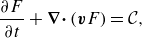 \begin{equation} \frac {\partial F}{\partial t} + {\boldsymbol{\nabla }} {\boldsymbol\cdot} \left ( {{\boldsymbol{v}} F} \right ) = {\mathcal C} , \end{equation}
where ${\boldsymbol{v}} = {\boldsymbol{v}}_g + (q {\boldsymbol{E}} + m {\boldsymbol{g}})/c_f$
, and the collision term on the right-hand side satisfies
${\boldsymbol{v}} = {\boldsymbol{v}}_g + (q {\boldsymbol{E}} + m {\boldsymbol{g}})/c_f$
, and the collision term on the right-hand side satisfies $\int _{-\infty }^{\infty }{{\mathcal C}(q) \, \textrm {d} q} = \int _{-\infty }^{\infty }{q\, {\mathcal C}(q) \, \textrm {d} q} = 0$
, expressing the conservation of the number and charge of the particles in collisions. The collision term can be decomposed as
$\int _{-\infty }^{\infty }{{\mathcal C}(q) \, \textrm {d} q} = \int _{-\infty }^{\infty }{q\, {\mathcal C}(q) \, \textrm {d} q} = 0$
, expressing the conservation of the number and charge of the particles in collisions. The collision term can be decomposed as ${\mathcal C}(q)={\mathcal C}^-(q) + {\mathcal C}^+(q)$
, with
${\mathcal C}(q)={\mathcal C}^-(q) + {\mathcal C}^+(q)$
, with
 \begin{equation} {\mathcal C}^-(q) =-\frac {4 \unicode{x03C0} a^2 E}{c_f} F(q) \int _{-\infty }^{\infty }{|q-r|\, F(r) \, \textrm {d} r} \end{equation}
and
 \begin{align} {\mathcal C}^+(q) &={} \frac {1}{2} \int _{-\infty }^{\infty } \int _{-\infty }^{\infty } \int _0^{2 a} \frac {|q_1-q_2|\, E}{c_f}\, F(q_1)\, F(q_2) \nonumber \\ &\quad {}\times \left [ { \delta \left ( {\frac {q_1 + q_2}{2} + q_{_E} - q}\right ) + \delta \left ( {\frac {q_1 + q_2}{2} - q_{_E} -q}\right ) }\right ] 2 \unicode{x03C0} e \, \textrm {d} e \, \textrm {d} q_1 \, \textrm {d} q_2 , \end{align}
where $E=|{\boldsymbol{E}}|$
and, for brevity, only the first argument of
$E=|{\boldsymbol{E}}|$
and, for brevity, only the first argument of $F$
is explicitly indicated.
$F$
is explicitly indicated.
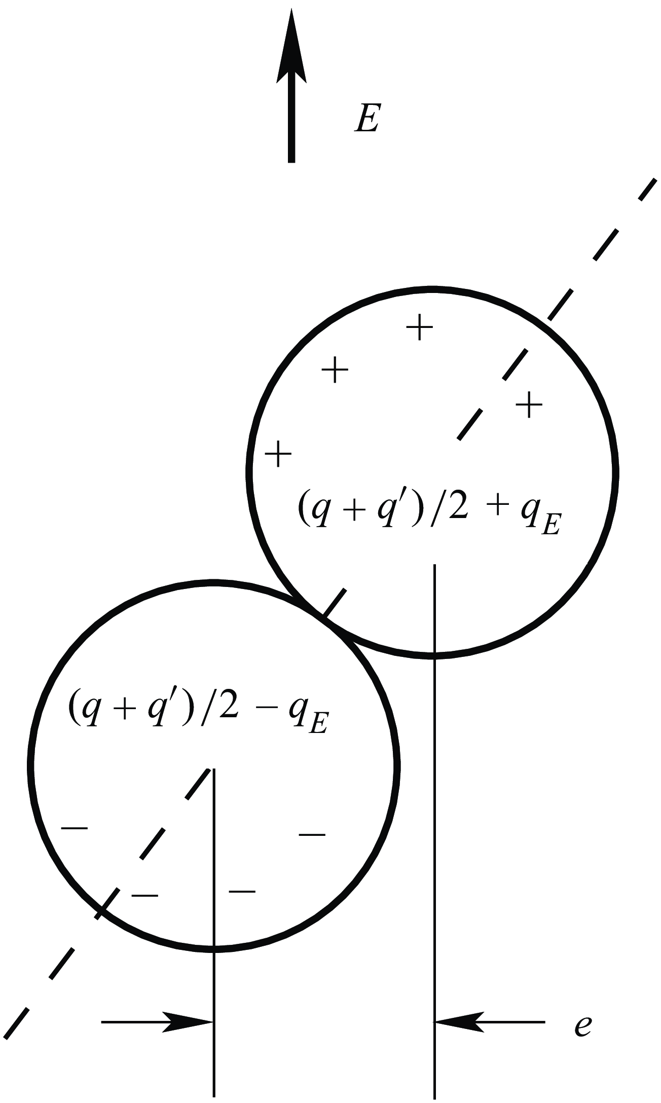
Figure 1. Charge redistribution in a collision.
In (2.2), ${\mathcal C}^-$
is the rate at which collisions between particles with charge
${\mathcal C}^-$
is the rate at which collisions between particles with charge $q$
and with any other charge
$q$
and with any other charge $r$
deplete the population of the former. Here,
$r$
deplete the population of the former. Here, $E\, |q-r|/c_f=|{\boldsymbol{v}}(q)-{\boldsymbol{v}}(r)|$
is the relative velocity of these particles, and
$E\, |q-r|/c_f=|{\boldsymbol{v}}(q)-{\boldsymbol{v}}(r)|$
is the relative velocity of these particles, and $4 \unicode{x03C0} a^2$
is the collision cross-section, so the factor
$4 \unicode{x03C0} a^2$
is the collision cross-section, so the factor $4 \unicode{x03C0} a^2 E\, |q-r|/c_f$
is the volume swept per unit time by a particle with charge
$4 \unicode{x03C0} a^2 E\, |q-r|/c_f$
is the volume swept per unit time by a particle with charge $q$
in its motion relative to particles with charge
$q$
in its motion relative to particles with charge $r$
. The product of this factor and
$r$
. The product of this factor and $F(r)$
is the mean number of collisions of this type that a particle with charge
$F(r)$
is the mean number of collisions of this type that a particle with charge $q$
undergoes per unit time, and the factor
$q$
undergoes per unit time, and the factor $F(q)$
accounts for the collisions of all the particles with charge
$F(q)$
accounts for the collisions of all the particles with charge $q$
in the unit volume.
$q$
in the unit volume.
In (2.3), ${\mathcal C}^+$
is the rate at which collisions replenish the population of particles with charge
${\mathcal C}^+$
is the rate at which collisions replenish the population of particles with charge $q$
. The collision of two particles with charges
$q$
. The collision of two particles with charges $q_1$
and
$q_1$
and $q_2$
generates two particles with charges
$q_2$
generates two particles with charges $(q_1+q_2)/2+q_{_E}$
and
$(q_1+q_2)/2+q_{_E}$
and $(q_1+q_2)/2-q_{_E}$
, with
$(q_1+q_2)/2-q_{_E}$
, with $q_{_E}=\gamma \epsilon _0 a^2 E \sqrt {1-(e/2 a)^2}$
in terms of the impact parameter
$q_{_E}=\gamma \epsilon _0 a^2 E \sqrt {1-(e/2 a)^2}$
in terms of the impact parameter $e$
in figure 1. Integration over
$e$
in figure 1. Integration over $q_1$
and
$q_1$
and $q_2$
accounts for all possible collisions, while the
$q_2$
accounts for all possible collisions, while the $\delta$
functions select those for which one of the particles emerges with charge
$\delta$
functions select those for which one of the particles emerges with charge $q$
, and the factor
$q$
, and the factor $1/2$
prevents counting each collision twice.
$1/2$
prevents counting each collision twice.
Using again a subscript $c$
to denote characteristic values of the variables, calling
$c$
to denote characteristic values of the variables, calling $L$
the characteristic size of the suspension (the interelectrode distance in the EPS cell described below), and assuming that the electric force plays a relevant role in the streaming of the particles so the estimation
$L$
the characteristic size of the suspension (the interelectrode distance in the EPS cell described below), and assuming that the electric force plays a relevant role in the streaming of the particles so the estimation $v_c=q_c E_c/c_f$
can be used, the orders of magnitude of the transport term on the left-hand side of (2.1) and each part of the collision term on the right-hand side are
$v_c=q_c E_c/c_f$
can be used, the orders of magnitude of the transport term on the left-hand side of (2.1) and each part of the collision term on the right-hand side are ${\boldsymbol{\nabla }} {\boldsymbol\cdot} ( {{\boldsymbol{v}} F} ) \sim q_c E_c F_c/(c_f L)$
and
${\boldsymbol{\nabla }} {\boldsymbol\cdot} ( {{\boldsymbol{v}} F} ) \sim q_c E_c F_c/(c_f L)$
and ${\mathcal C}^{\pm } \sim a^2 E_c q_c^2 F_c^2/c_f$
, so
${\mathcal C}^{\pm } \sim a^2 E_c q_c^2 F_c^2/c_f$
, so ${\mathcal C}^{\pm }/{\boldsymbol{\nabla }} {\boldsymbol\cdot} ({\boldsymbol{v}} F) \sim a^2 L n_c$
, with
${\mathcal C}^{\pm }/{\boldsymbol{\nabla }} {\boldsymbol\cdot} ({\boldsymbol{v}} F) \sim a^2 L n_c$
, with $n_c=q_c F_c$
. This is also the order of the ratio of the characteristic size of the suspension to the mean free path of the particles between collisions,
$n_c=q_c F_c$
. This is also the order of the ratio of the characteristic size of the suspension to the mean free path of the particles between collisions, $\lambda \sim 1/(n_c a^2)$
.
$\lambda \sim 1/(n_c a^2)$
.
In the continuum regime when this ratio is large, a typical particle collides many times with its neighbours before travelling a distance of order $L$
, approaching a state of equilibrium with them. Each of
$L$
, approaching a state of equilibrium with them. Each of ${\mathcal C}^-(q)$
and
${\mathcal C}^-(q)$
and ${\mathcal C}^+(q)$
is large compared with the transport term on the left-hand side of (2.1), so the equation reduces to
${\mathcal C}^+(q)$
is large compared with the transport term on the left-hand side of (2.1), so the equation reduces to ${\mathcal C}^-(q) + {\mathcal C}^+(q)=0$
at leading order in a Chapman–Enskog expansion of the distribution function of the form
${\mathcal C}^-(q) + {\mathcal C}^+(q)=0$
at leading order in a Chapman–Enskog expansion of the distribution function of the form $F=F_{eq}[1+O(\lambda /L)]$
. This is an integral equation whose solution (the equilibrium distribution function) can be computed for given values of the electric field and the number and charge densities,
$F=F_{eq}[1+O(\lambda /L)]$
. This is an integral equation whose solution (the equilibrium distribution function) can be computed for given values of the electric field and the number and charge densities, $n=\int _{-\infty }^{\infty }{F(q) \, \textrm {d} q}$
and
$n=\int _{-\infty }^{\infty }{F(q) \, \textrm {d} q}$
and $\rho _e=\int _{-\infty }^{\infty }{q F(q) \, \textrm {d} q}$
, which are the magnitudes conserved in the collisions. In terms of the mean particle charge
$\rho _e=\int _{-\infty }^{\infty }{q F(q) \, \textrm {d} q}$
, which are the magnitudes conserved in the collisions. In terms of the mean particle charge $\overline {q}=\rho _e/n$
, the solution is of the form (see Ling & Higuera Reference Ling and Higuera2022)
$\overline {q}=\rho _e/n$
, the solution is of the form (see Ling & Higuera Reference Ling and Higuera2022)
 \begin{equation} F_{eq}(q; E, n, \overline {q}) = \frac {n}{\gamma \epsilon _0 a^2 E}\, G \left ( {\frac {q-\overline {q}}{\gamma \epsilon _0 a^2 E} }\right ) , \end{equation}
where the function $G$
, computed by discretising and numerically solving the integral equation, is shown by the dashed curves in figure 2 below.
$G$
, computed by discretising and numerically solving the integral equation, is shown by the dashed curves in figure 2 below.
2.2. The EPS cell
As was mentioned in the Introduction, the core of an EPS cell is the gap between two parallel horizontal electrodes spaced a distance $L$
apart. The gap contains a certain number of small particles of large electrical conductivity,
$L$
apart. The gap contains a certain number of small particles of large electrical conductivity, $N$
per unit electrode area, and a direct current voltage
$N$
per unit electrode area, and a direct current voltage $V$
is applied to the lower electrode relative to the upper one. The electric field at the lower electrode,
$V$
is applied to the lower electrode relative to the upper one. The electric field at the lower electrode, $E(0)$
say, induces a charge
$E(0)$
say, induces a charge $q_+=\alpha \epsilon _0 a^2\, E(0)$
at each particle in contact with the electrode (Maxwell Reference Maxwell1881), and exerts a vertical force
$q_+=\alpha \epsilon _0 a^2\, E(0)$
at each particle in contact with the electrode (Maxwell Reference Maxwell1881), and exerts a vertical force $\beta \epsilon _0 a^2\, E(0)^2$
on the particle (Lebedev & Skal’skaya Reference Lebedev and Skal’skaya1962). Here,
$\beta \epsilon _0 a^2\, E(0)^2$
on the particle (Lebedev & Skal’skaya Reference Lebedev and Skal’skaya1962). Here, $\alpha =2 \unicode{x03C0} ^3/3 \approx 20.67$
and
$\alpha =2 \unicode{x03C0} ^3/3 \approx 20.67$
and $\beta \approx 17.20$
. The particle detaches from the electrode when this force overcomes the sum of its weight
$\beta \approx 17.20$
. The particle detaches from the electrode when this force overcomes the sum of its weight $m g$
and its adhesion force to the electrode
$m g$
and its adhesion force to the electrode $A$
. This condition determines the minimum value of
$A$
. This condition determines the minimum value of $E(0)$
required for particle suspension,
$E(0)$
required for particle suspension, $E(0) \gt E_m = \sqrt {(mg + A)/(\beta \epsilon _0 a^2)}$
, which in turn determines the minimum required voltage
$E(0) \gt E_m = \sqrt {(mg + A)/(\beta \epsilon _0 a^2)}$
, which in turn determines the minimum required voltage $V_m=E_m L$
, because the electric field is uniform in the gap at the onset of particle suspension. If this condition is satisfied, then, as mentioned above, the particles detach from the electrode, drift across the gap, and eventually hit the upper electrode. There, calling
$V_m=E_m L$
, because the electric field is uniform in the gap at the onset of particle suspension. If this condition is satisfied, then, as mentioned above, the particles detach from the electrode, drift across the gap, and eventually hit the upper electrode. There, calling $E(L)$
the electric field at this electrode, the particles instantly acquire the negative charge
$E(L)$
the electric field at this electrode, the particles instantly acquire the negative charge $q_-=-\alpha \epsilon _0 a^2\, E(L)$
and experience the (downward) force
$q_-=-\alpha \epsilon _0 a^2\, E(L)$
and experience the (downward) force $-\beta \epsilon _0 a^2\, E(L)^2$
, which, together with their weight, makes the particles fall.
$-\beta \epsilon _0 a^2\, E(L)^2$
, which, together with their weight, makes the particles fall.
The forces acting on a flying particle with charge $q$
include the electric force
$q$
include the electric force $q {\boldsymbol{E}}$
(when the distance to the electrodes is large compared with the particle radius), the weight
$q {\boldsymbol{E}}$
(when the distance to the electrodes is large compared with the particle radius), the weight $m {\boldsymbol{g}}$
, and the hydrodynamic drag of the gas,
$m {\boldsymbol{g}}$
, and the hydrodynamic drag of the gas, $-c_f ({\boldsymbol{v}}-{\boldsymbol{v}}_g)$
. In the absence of particle inertia, the balance of these forces determines the particle velocity mentioned above.
$-c_f ({\boldsymbol{v}}-{\boldsymbol{v}}_g)$
. In the absence of particle inertia, the balance of these forces determines the particle velocity mentioned above.
In stationary conditions, and in the absence of inflow or outflow of particles to the gap, the flux of particles moving upwards across any horizontal section of the gap must equal the flux of particles moving downwards. Owing to their weight, the upward moving particles, which necessarily bear positive charges, move more slowly and therefore are more numerous than the downward moving particles, which bear smaller or negative charges. This leads to a space charge density in the gap with the polarity of the lower electrode (positive if $V\gt 0$
). The electric field induced by this charge points downwards in the lower part of the gap, opposing the field due to the applied voltage, and upwards in the upper part, enhancing the field of the applied voltage.
$V\gt 0$
). The electric field induced by this charge points downwards in the lower part of the gap, opposing the field due to the applied voltage, and upwards in the upper part, enhancing the field of the applied voltage.
The space charge sets an upper bound to the number $N$
of particles that can be suspended per unit electrode area for a given voltage (Zhebelev Reference Zhebelev1992). The space charge induced field increases with
$N$
of particles that can be suspended per unit electrode area for a given voltage (Zhebelev Reference Zhebelev1992). The space charge induced field increases with $N$
, which reduces the net field at the lower electrode, until it falls to
$N$
, which reduces the net field at the lower electrode, until it falls to $E_m$
and the electric force on the particles in contact with this electrode can no longer overcome the particle weight and the adhesion force. Thus for a given voltage higher than
$E_m$
and the electric force on the particles in contact with this electrode can no longer overcome the particle weight and the adhesion force. Thus for a given voltage higher than $V_m$
, the value of
$V_m$
, the value of $N$
may range between zero and a certain maximum
$N$
may range between zero and a certain maximum $N_{max}$
. The maximum
$N_{max}$
. The maximum $N$
is attained in the normal operation of the device, when there is an excess of particles deposited on the lower electrode. It increases when the voltage is increased. A limit to the voltage, and thus to
$N$
is attained in the normal operation of the device, when there is an excess of particles deposited on the lower electrode. It increases when the voltage is increased. A limit to the voltage, and thus to $N$
, is due to the onset of electric breakdown of the gas in the regions of highest electric field, though this issue will not be discussed here.
$N$
, is due to the onset of electric breakdown of the gas in the regions of highest electric field, though this issue will not be discussed here.
Using $N/L$
as a coarse estimation of the number density of particles, the mean free path of the suspended particles is
$N/L$
as a coarse estimation of the number density of particles, the mean free path of the suspended particles is $\lambda \sim L/(N a^2)$
. This becomes of the order of the interelectrode distance for
$\lambda \sim L/(N a^2)$
. This becomes of the order of the interelectrode distance for $N \sim a^{-2}$
, a value that, up to numerical factors, would amount to full coverage of the lower electrode by a monolayer of particles, should these particles be deposited on it. But such values of
$N \sim a^{-2}$
, a value that, up to numerical factors, would amount to full coverage of the lower electrode by a monolayer of particles, should these particles be deposited on it. But such values of $N$
are still compatible with the assumption of a dilute suspension if the particles are suspended and
$N$
are still compatible with the assumption of a dilute suspension if the particles are suspended and $L \gg a$
.
$L \gg a$
.
The electric field induced by the charged particles can also be estimated. Consider first the suspension in the absence of particle collisions. Each particle conserves the charge that it acquired in its last contact with an electrode, which was of order $\epsilon _0 a^2 V/L$
up to a numerical factor. In these conditions, the charge density in the gap can be expected to be
$\epsilon _0 a^2 V/L$
up to a numerical factor. In these conditions, the charge density in the gap can be expected to be $\rho _e \sim (N/L) \epsilon _0 a^2 V/L$
, and the electric field induced by this charge is
$\rho _e \sim (N/L) \epsilon _0 a^2 V/L$
, and the electric field induced by this charge is $E_{sc} \sim N a^2 V/L$
(from Gauss’ law
$E_{sc} \sim N a^2 V/L$
(from Gauss’ law ${\boldsymbol{\nabla }} {\boldsymbol\cdot} {\boldsymbol{E}} = \rho _e/\epsilon _0$
). The condition that this field be of the order of the field
${\boldsymbol{\nabla }} {\boldsymbol\cdot} {\boldsymbol{E}} = \rho _e/\epsilon _0$
). The condition that this field be of the order of the field $V/L$
due to the applied voltage provides the estimation
$V/L$
due to the applied voltage provides the estimation $N_{max} \sim a^{-2}$
for the maximum value of
$N_{max} \sim a^{-2}$
for the maximum value of $N$
. This voltage-independent estimation coincides with the one above for the mean free path to be of the order of the interelectrode distance, and suggests that the condition
$N$
. This voltage-independent estimation coincides with the one above for the mean free path to be of the order of the interelectrode distance, and suggests that the condition $\lambda \ll L$
is never attained.
$\lambda \ll L$
is never attained.
However, the estimation of the charge density used above breaks down when collisions between particles are frequent events. The exchanges of charge in the collisions drive the suspension toward quasi-neutrality in most of the gap (keeping a dispersion of particle charges of order $q_{_E}$
), which makes the charge density smaller than estimated, and allows larger values of
$q_{_E}$
), which makes the charge density smaller than estimated, and allows larger values of $N$
to be attained before the space charge induced field becomes of order
$N$
to be attained before the space charge induced field becomes of order $V/L$
. Thus quasi-neutrality of the suspension opens the way to a continuum regime, which can be expected for values of
$V/L$
. Thus quasi-neutrality of the suspension opens the way to a continuum regime, which can be expected for values of $V$
large compared with
$V$
large compared with $V_m$
and values
$V_m$
and values $N \gg a^{-2}$
. When
$N \gg a^{-2}$
. When $V \gg V_m$
, the condition that the field at the lower electrode should approach
$V \gg V_m$
, the condition that the field at the lower electrode should approach $E_m$
when
$E_m$
when $N$
approaches its maximum value implies that the space charge induced field is largely offsetting the field due to the applied voltage. The field in most of the gap is still of order
$N$
approaches its maximum value implies that the space charge induced field is largely offsetting the field due to the applied voltage. The field in most of the gap is still of order $V/L \gg E_m$
(actually larger than
$V/L \gg E_m$
(actually larger than $V/L$
in the upper part of the gap). The charges that individual particles acquire in collisions with other particles are therefore of order
$V/L$
in the upper part of the gap). The charges that individual particles acquire in collisions with other particles are therefore of order $q_{_E}=O(\epsilon _0 a^2 V/L)$
. Since collisions are very frequent in the continuum regime, a particle that emerges from a collision with an excess of charge of order
$q_{_E}=O(\epsilon _0 a^2 V/L)$
. Since collisions are very frequent in the continuum regime, a particle that emerges from a collision with an excess of charge of order $q_{_E}$
may emerge from another with a defect of charge of order
$q_{_E}$
may emerge from another with a defect of charge of order $-q_{_E}$
. Quasi-neutrality of the suspension is due to the near cancellation of the contributions of positive and negative particles to the mean particle charge, not to the charges of individual particles being small.
$-q_{_E}$
. Quasi-neutrality of the suspension is due to the near cancellation of the contributions of positive and negative particles to the mean particle charge, not to the charges of individual particles being small.
An order-of-magnitude estimation of the charge density is not easy to obtain in these conditions ( $V/V_m \gg 1$
with
$V/V_m \gg 1$
with $E=O(E_m)$
at the lower electrode), because the charge density is then far from uniform across the gap (see Shoshin & Dreizin Reference Shoshin and Dreizin2002). This, in turn, precludes an estimation of the maximum
$E=O(E_m)$
at the lower electrode), because the charge density is then far from uniform across the gap (see Shoshin & Dreizin Reference Shoshin and Dreizin2002). This, in turn, precludes an estimation of the maximum $N$
that can be attained for a given voltage. To assess the extent to which quasi-neutrality and the continuum regime are realised, and to compute the maximum
$N$
that can be attained for a given voltage. To assess the extent to which quasi-neutrality and the continuum regime are realised, and to compute the maximum $N$
, stationary one-dimensional solutions of (2.1), together with the Poisson equation
$N$
, stationary one-dimensional solutions of (2.1), together with the Poisson equation $\nabla ^2 \phi =-\rho _e/\epsilon _0$
for the electric potential
$\nabla ^2 \phi =-\rho _e/\epsilon _0$
for the electric potential $\phi$
, with
$\phi$
, with ${\boldsymbol{E}}=-{\boldsymbol{\nabla }} \phi$
, have been computed numerically in the gap between two infinite horizontal electrodes for various values of the voltage well above the minimum required for electric forces to suspend particles, and values of
${\boldsymbol{E}}=-{\boldsymbol{\nabla }} \phi$
, have been computed numerically in the gap between two infinite horizontal electrodes for various values of the voltage well above the minimum required for electric forces to suspend particles, and values of $N$
well above the value
$N$
well above the value $a^{-2}$
for which collisions between particles first come into play according to the estimations of the previous paragraphs. These solutions are compared with the equilibrium distribution function (2.4) to quantify the approach to equilibrium.
$a^{-2}$
for which collisions between particles first come into play according to the estimations of the previous paragraphs. These solutions are compared with the equilibrium distribution function (2.4) to quantify the approach to equilibrium.
Calling $x$
the distance measured upwards from the lower electrode, the solutions sought are of the form
$x$
the distance measured upwards from the lower electrode, the solutions sought are of the form $F(q, x)$
,
$F(q, x)$
, $\phi (x)$
. The gas in the closed gap is quiescent in these conditions, the electric force transferred to the gas by the inertialess particles being balanced by a vertical pressure gradient. The velocities of the particles are also vertical, of value
$\phi (x)$
. The gas in the closed gap is quiescent in these conditions, the electric force transferred to the gas by the inertialess particles being balanced by a vertical pressure gradient. The velocities of the particles are also vertical, of value $v_x=(q E - mg)/c_f$
.
$v_x=(q E - mg)/c_f$
.
The following boundary conditions are imposed:
 \begin{equation} \left . { \begin{gathered} F(q,0) = F_+ \delta (q-q_+) \quad \mbox{for} \ v_x\gt 0, \quad \mbox{with} \ F_+ \frac {q_+ E-mg}{c_f}=-\int _{v_x\lt 0}{v_x F \, \textrm {d} q}, \\ \phi = V, \end{gathered} } \right \} \end{equation}
at the lower electrode $x=0$
,
$x=0$
,
 \begin{equation} \left . { \begin{gathered} F(q,L) = F_- \delta (q-q_-) \quad \mbox{for} \ v_x\lt 0, \quad \mbox{with} \ F_- \frac {q_- E-mg}{c_f}=-\int _{v_x\gt 0}{v_x F \, \textrm {d} q}, \\ \phi = 0, \end{gathered} } \right \} \end{equation}
at the upper electrode $x=L$
, and
$x=L$
, and
 \begin{equation} \int _0^L \int _{-\infty }^{\infty }{F(q,x) \, \textrm {d} q \, \textrm {d} x} = N . \end{equation}
The first lines of (2.5) and (2.6) express the conditions that the particles reaching each electrode are re-emitted with charges $q_+=\alpha \epsilon _0 a^2\, E(0)$
and
$q_+=\alpha \epsilon _0 a^2\, E(0)$
and $q_-=-\alpha \epsilon _0 a^2\, E(L)$
, and the velocities corresponding to these charges, in such a manner that the total number of particles per unit electrode area is conserved, equal to the value of
$q_-=-\alpha \epsilon _0 a^2\, E(L)$
, and the velocities corresponding to these charges, in such a manner that the total number of particles per unit electrode area is conserved, equal to the value of $N$
in (2.7).
$N$
in (2.7).
It may be noted that the parameter $\beta$
and the adhesion force
$\beta$
and the adhesion force $A$
do not appear in this formulation. Apparently a solution may exist whenever
$A$
do not appear in this formulation. Apparently a solution may exist whenever $v_x(q_+)=(q_+ E(0) - mg)/c_f \gt 0$
, a condition that can be satisfied for sufficiently small values of
$v_x(q_+)=(q_+ E(0) - mg)/c_f \gt 0$
, a condition that can be satisfied for sufficiently small values of $N$
provided that
$N$
provided that $V\gt (m g/\alpha \epsilon _0)^{1/2} L/a$
. A more detailed analysis of the rebound of the particles at the lower electrode might modify this conclusion. While an account of the particle–electrode interaction may be very complex and is beyond the scope of this work, two limiting cases are briefly discussed here. In the absence of inertial effects, lubrication theory determines the hydrodynamic force retarding the motion of a falling particle at a distance
$V\gt (m g/\alpha \epsilon _0)^{1/2} L/a$
. A more detailed analysis of the rebound of the particles at the lower electrode might modify this conclusion. While an account of the particle–electrode interaction may be very complex and is beyond the scope of this work, two limiting cases are briefly discussed here. In the absence of inertial effects, lubrication theory determines the hydrodynamic force retarding the motion of a falling particle at a distance $x \ll a$
from the lower electrode as
$x \ll a$
from the lower electrode as $F_p=3 \unicode{x03C0} \mu _g a^2 v_p/8 x$
, due to the squeezing of the gas film between particle and electrode. Here,
$F_p=3 \unicode{x03C0} \mu _g a^2 v_p/8 x$
, due to the squeezing of the gas film between particle and electrode. Here, $v_p$
is the instantaneous velocity of the particle. The balance of this force and the attractive van der Waals force
$v_p$
is the instantaneous velocity of the particle. The balance of this force and the attractive van der Waals force $H a/(24 x^2)$
, where
$H a/(24 x^2)$
, where $H$
is the Hamaker constant (Israelachvili Reference Israelachvili1992), gives
$H$
is the Hamaker constant (Israelachvili Reference Israelachvili1992), gives $v_p=H/(9 \unicode{x03C0} \mu _g a x)$
, suggesting that the particle will be trapped by the electrode and can be resuspended only if the electric field at the electrode surface is larger than
$v_p=H/(9 \unicode{x03C0} \mu _g a x)$
, suggesting that the particle will be trapped by the electrode and can be resuspended only if the electric field at the electrode surface is larger than $E_m$
. On the other hand, if the inertia of the particle matters in the last stage of its approach to the electrode (or in a longer stage in the case
$E_m$
. On the other hand, if the inertia of the particle matters in the last stage of its approach to the electrode (or in a longer stage in the case $t_{coll}/t_{s} \ll 1$
discussed in the following section), then the particle may rebound even in the absence of electric forces. Calling
$t_{coll}/t_{s} \ll 1$
discussed in the following section), then the particle may rebound even in the absence of electric forces. Calling $v_{p_i}$
the velocity of the falling particle before it enters the range of attractive forces, an energy balance (see e.g. Friedlander Reference Friedlander2000) determines the condition for the particle to rebound as
$v_{p_i}$
the velocity of the falling particle before it enters the range of attractive forces, an energy balance (see e.g. Friedlander Reference Friedlander2000) determines the condition for the particle to rebound as $v_{p_i}^2 \gt v_{cr}^2 = 2 (1-e_r^2) (-\Phi _0)/m e_r^2$
, where
$v_{p_i}^2 \gt v_{cr}^2 = 2 (1-e_r^2) (-\Phi _0)/m e_r^2$
, where $e_r$
is a restitution coefficient, and
$e_r$
is a restitution coefficient, and $\Phi _0\lt 0$
is the potential of the attractive forces at the electrode surface. When this condition is satisfied, the particle rebounds with velocity
$\Phi _0\lt 0$
is the potential of the attractive forces at the electrode surface. When this condition is satisfied, the particle rebounds with velocity $v_{p_o}=v_{p_i} e_r (1-v_{cr}^2/v_{p_i}^2)^{1/2}$
. Later, the drag of the gas, whose effect has been left out in the rebound, slows down the particle, and would force it to fall back on the electrode if the electric field is smaller than the value
$v_{p_o}=v_{p_i} e_r (1-v_{cr}^2/v_{p_i}^2)^{1/2}$
. Later, the drag of the gas, whose effect has been left out in the rebound, slows down the particle, and would force it to fall back on the electrode if the electric field is smaller than the value $m g/q_+$
required for the electric force to overcome the particle weight. This field is smaller than
$m g/q_+$
required for the electric force to overcome the particle weight. This field is smaller than $E_m$
and does not depend directly on the adhesion force.
$E_m$
and does not depend directly on the adhesion force.
Coming back to the stationary one-dimensional problem posed in the previous paragraphs, the variables $(x, v_x, \phi , q, F)$
are non-dimensionalised with
$(x, v_x, \phi , q, F)$
are non-dimensionalised with $[L, mg/c_f, E_0 L, q_0, 1/(\alpha L a^2 q_0)]$
, where
$[L, mg/c_f, E_0 L, q_0, 1/(\alpha L a^2 q_0)]$
, where $E_0=\sqrt {m g/\alpha \epsilon _0 a^2}$
and
$E_0=\sqrt {m g/\alpha \epsilon _0 a^2}$
and $q_0 E_0 = m g$
, so
$q_0 E_0 = m g$
, so $N$
is scaled with
$N$
is scaled with $1/(\alpha a^2)$
. These dimensionless variables are denoted with the same symbols used before for their dimensional counterparts.
$1/(\alpha a^2)$
. These dimensionless variables are denoted with the same symbols used before for their dimensional counterparts.
Note, in particular, that the dimensionless voltage $V$
in the dimensionless form of (2.5) is the ratio of the interelectrode voltage to the minimum value
$V$
in the dimensionless form of (2.5) is the ratio of the interelectrode voltage to the minimum value $E_0 L$
for which the particles can be kept suspended in the absence of adhesion forces. And up to a factor
$E_0 L$
for which the particles can be kept suspended in the absence of adhesion forces. And up to a factor $\alpha$
,
$\alpha$
, $N$
is the ratio of the number of suspended particles per unit electrode area to the value
$N$
is the ratio of the number of suspended particles per unit electrode area to the value $a^{-2}$
of this magnitude for which
$a^{-2}$
of this magnitude for which $\lambda \sim L$
and collisions between particles first come into play.
$\lambda \sim L$
and collisions between particles first come into play.
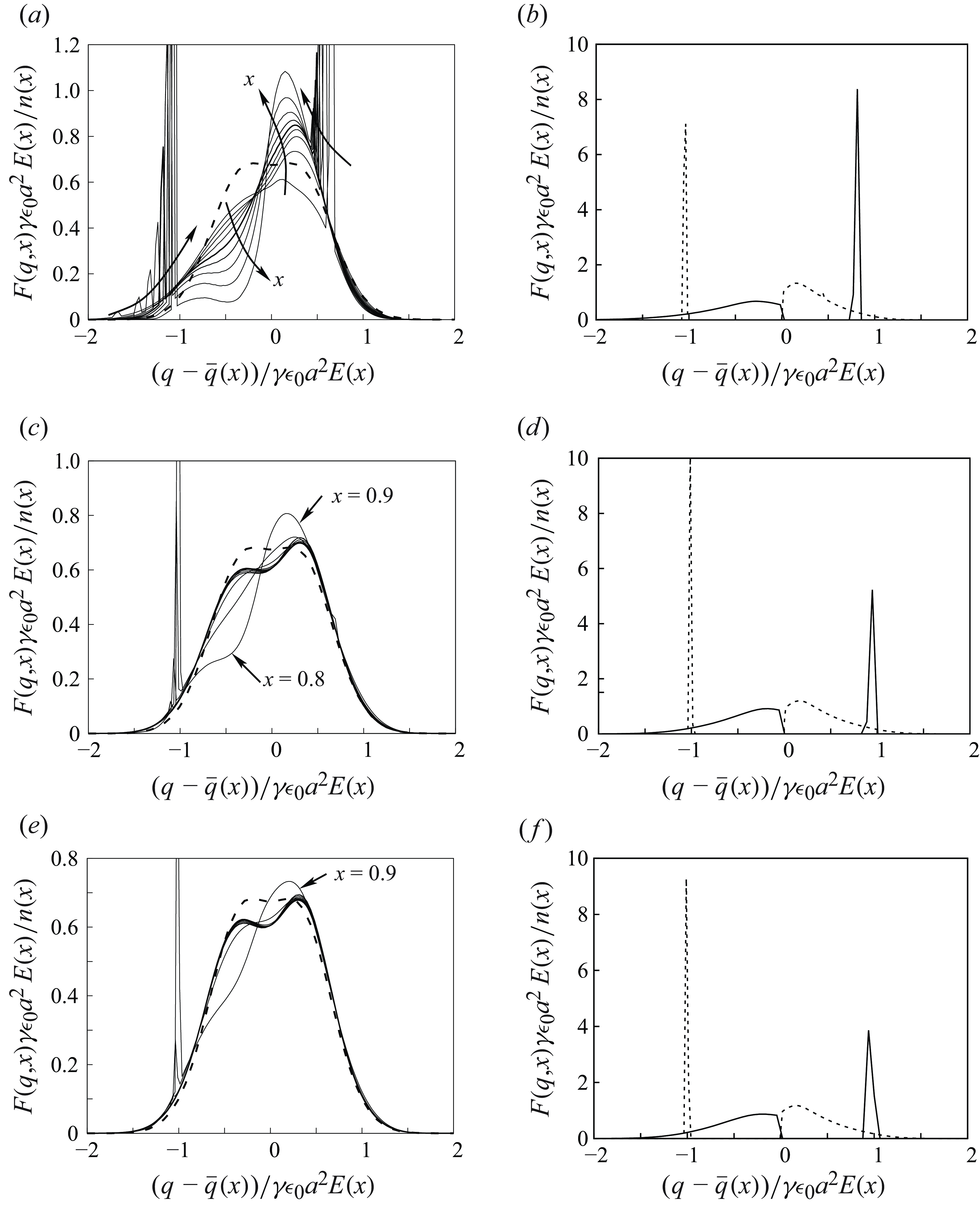
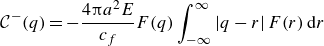
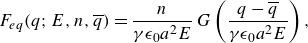
Figure 2. Distribution function scaled with the local values of $n(x)$
,
$n(x)$
, $\overline {q}(x)$
and
$\overline {q}(x)$
and $E(x)$
, for (a,b)
$E(x)$
, for (a,b) $(V, N)=(4, 9)$
, (c,d)
$(V, N)=(4, 9)$
, (c,d) $(V, N)=(8, 43)$
, and (e, f)
$(V, N)=(8, 43)$
, and (e, f) $(V, N)=(10, 75)$
. (a,c,e) The scaled distribution function at nine equispaced values of
$(V, N)=(10, 75)$
. (a,c,e) The scaled distribution function at nine equispaced values of $x$
between 0.1 and 0.9. (b,d, f) The same function at the lower electrode (
$x$
between 0.1 and 0.9. (b,d, f) The same function at the lower electrode ( $x=0$
, solid) and the upper electrode (
$x=0$
, solid) and the upper electrode ( $x=1$
, dashed). In (
$x=1$
, dashed). In ( $a$
),
$a$
), $x$
increases as indicated by the arrows. In (
$x$
increases as indicated by the arrows. In ( $c$
) and (
$c$
) and ( $e$
), the results for different values of
$e$
), the results for different values of $x$
are very close to each other for most values of
$x$
are very close to each other for most values of $x$
, except for
$x$
, except for $x=0.8$
and 0.9, which are marked by arrows. The dashed curves in (a,c,e) show the equilibrium distribution function scaled as in (2.4).
$x=0.8$
and 0.9, which are marked by arrows. The dashed curves in (a,c,e) show the equilibrium distribution function scaled as in (2.4).
The variables $q$
and
$q$
and $x$
are discretised using finite differences, and the discretised equations are solved with a pseudo-transient iteration. The numerical method was described in Higuera (Reference Higuera2018).
$x$
are discretised using finite differences, and the discretised equations are solved with a pseudo-transient iteration. The numerical method was described in Higuera (Reference Higuera2018).
Figure 2 shows some results of these computations. The computed distribution function is rescaled as $F_{eq}$
in (2.4), using the local values of
$F_{eq}$
in (2.4), using the local values of $n(x)=\int _{-\infty }^{\infty }{F(q,x) \, \textrm {d} q}$
,
$n(x)=\int _{-\infty }^{\infty }{F(q,x) \, \textrm {d} q}$
, $\bar{q}{(x)}=n(x)^{-1} \int _{-\infty }^{\infty }{q\, F(q,x) \, \textrm {d} q}$
and
$\bar{q}{(x)}=n(x)^{-1} \int _{-\infty }^{\infty }{q\, F(q,x) \, \textrm {d} q}$
and $E(x)$
. It is displayed in figure 2(a,c,e) for nine equispaced values of
$E(x)$
. It is displayed in figure 2(a,c,e) for nine equispaced values of $x$
between 0.1 and 0.9, for
$x$
between 0.1 and 0.9, for $V=4$
,
$V=4$
, $N=9$
(figure 2
a),
$N=9$
(figure 2
a), $V=8$
,
$V=8$
, $N=43$
(figure 2
c), and
$N=43$
(figure 2
c), and $V=10$
,
$V=10$
, $N=75$
(figure 2
e). The dashed curves in these graphs show the scaled equilibrium distribution function
$N=75$
(figure 2
e). The dashed curves in these graphs show the scaled equilibrium distribution function $G$
in (2.4). The rescaled distribution function at the electrodes,
$G$
in (2.4). The rescaled distribution function at the electrodes, $x=0$
and 1, is shown separately in figure 2(b,d, f). The largest values of
$x=0$
and 1, is shown separately in figure 2(b,d, f). The largest values of $N$
for which a numerical solution has been obtained are approximately 10.5 for
$N$
for which a numerical solution has been obtained are approximately 10.5 for $V=4$
, 44 for
$V=4$
, 44 for $V=8$
, and 77 for
$V=8$
, and 77 for $V=10$
. The electric field at the lower electrode is rapidly approaching its minimum possible value, which is unity in dimensionless variables, when
$V=10$
. The electric field at the lower electrode is rapidly approaching its minimum possible value, which is unity in dimensionless variables, when $N$
is increased to these values.
$N$
is increased to these values.
As can be seen, the distribution function at the electrodes always differs from the equilibrium distribution function. The sharp peaks in the figures, specially at the electrodes, are due to the $\delta$
functions in (2.5) and (2.6), which are discretised on the numerical mesh. The slight shifts of the locations of these peaks are due to the variation of
$\delta$
functions in (2.5) and (2.6), which are discretised on the numerical mesh. The slight shifts of the locations of these peaks are due to the variation of $\overline {q}$
with
$\overline {q}$
with $x$
. When
$x$
. When $V=8$
and 10, the peaks smooth out away from the electrodes (though the peak originated at the upper electrode is significant in figure 2(c,e) for
$V=8$
and 10, the peaks smooth out away from the electrodes (though the peak originated at the upper electrode is significant in figure 2(c,e) for $x$
larger than approximately 0.7 and 0.8, respectively), and the distribution function approaches the equilibrium one in most of the cell. Some asymmetry is left, however, probably a remnant of the slow upward moving particles outnumbering the faster downward moving particles, as mentioned above. When
$x$
larger than approximately 0.7 and 0.8, respectively), and the distribution function approaches the equilibrium one in most of the cell. Some asymmetry is left, however, probably a remnant of the slow upward moving particles outnumbering the faster downward moving particles, as mentioned above. When $V=4$
, on the other hand, the peaks persist longer, and the distribution function nowhere approaches the equilibrium one.
$V=4$
, on the other hand, the peaks persist longer, and the distribution function nowhere approaches the equilibrium one.
These results are in line with the estimation above, that ${\mathcal C}^{\pm }/{\boldsymbol{\nabla }} {\boldsymbol\cdot} ({\boldsymbol{v}} F) \sim a^2 L n_c$
, as
${\mathcal C}^{\pm }/{\boldsymbol{\nabla }} {\boldsymbol\cdot} ({\boldsymbol{v}} F) \sim a^2 L n_c$
, as $a^2 L n_c$
is the dimensionless
$a^2 L n_c$
is the dimensionless $N$
up to a constant factor. Accounting for the scaling factors used in the non-dimensionalisation, a global Knudsen number
$N$
up to a constant factor. Accounting for the scaling factors used in the non-dimensionalisation, a global Knudsen number ${Kn}=\alpha /(4 \unicode{x03C0} N)$
can be defined, where
${Kn}=\alpha /(4 \unicode{x03C0} N)$
can be defined, where $1/N^{1/3}$
plays the role of the mean dimensionless distance between particles (
$1/N^{1/3}$
plays the role of the mean dimensionless distance between particles ( $4 \unicode{x03C0} a^2$
being the collision cross-section). Values of this number are 0.18 for
$4 \unicode{x03C0} a^2$
being the collision cross-section). Values of this number are 0.18 for $(V, N) = (4, 9)$
, 0.038 for
$(V, N) = (4, 9)$
, 0.038 for $(V, N) = (8, 43)$
, and 0.022 for
$(V, N) = (8, 43)$
, and 0.022 for $(V, N) = (10, 75)$
.
$(V, N) = (10, 75)$
.
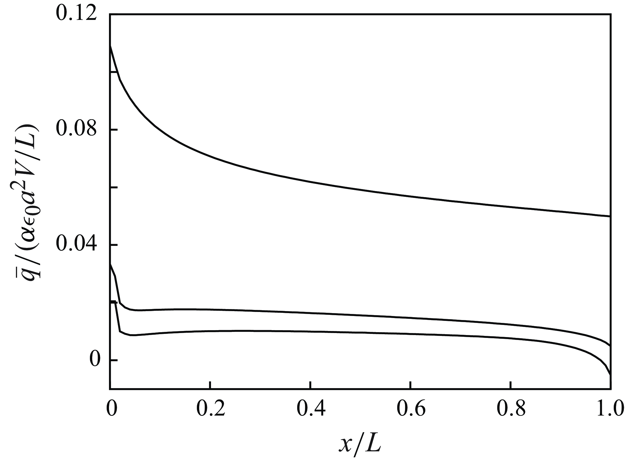
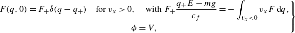
Figure 3. Distribution of mean charge $\overline {q}=\rho _e/n$
across the gap for
$\overline {q}=\rho _e/n$
across the gap for $(V, N)=(4, 9)$
,
$(V, N)=(4, 9)$
, $(8, 43)$
and
$(8, 43)$
and $(10, 75)$
, from top to bottom.
$(10, 75)$
, from top to bottom.
The mean particle charge $\overline {q}=\int _{-\infty }^{\infty }{q\, F(q) \, \textrm {d} q}$
, scaled with
$\overline {q}=\int _{-\infty }^{\infty }{q\, F(q) \, \textrm {d} q}$
, scaled with $\alpha \epsilon _0 a^2 V/L$
, is shown in figure 3 as a function of
$\alpha \epsilon _0 a^2 V/L$
, is shown in figure 3 as a function of $x$
for the three pairs of values of the dimensionless parameters (
$x$
for the three pairs of values of the dimensionless parameters ( $V,N$
) in figure 2. The scaling factor
$V,N$
) in figure 2. The scaling factor $\alpha \epsilon _0 a^2 V/L$
is of the order of the charge acquired by a particle in a collision with another particle or with the upper electrode, so the results in this figure show the extent of the cancellation of the contributions of positive and negative particles to the mean particle charge. Clearly, the suspension is approaching quasi-neutrality in a plateau that covers most of the gap when
$\alpha \epsilon _0 a^2 V/L$
is of the order of the charge acquired by a particle in a collision with another particle or with the upper electrode, so the results in this figure show the extent of the cancellation of the contributions of positive and negative particles to the mean particle charge. Clearly, the suspension is approaching quasi-neutrality in a plateau that covers most of the gap when $V$
increases, with
$V$
increases, with $N$
of the order of its maximum possible value,
$N$
of the order of its maximum possible value, $N_{max}(V)$
. To the resolution of these computations, the scaled mean particle charge is small also in the thin Knudsen layers by the electrodes where the mean free path is not small compared with the distance to the nearest electrode. These results substantiate the estimations above, linking equilibrium and quasi-neutrality.
$N_{max}(V)$
. To the resolution of these computations, the scaled mean particle charge is small also in the thin Knudsen layers by the electrodes where the mean free path is not small compared with the distance to the nearest electrode. These results substantiate the estimations above, linking equilibrium and quasi-neutrality.
Figure 4 shows sample distributions of the dimensionless electric field for two values of the voltage and various values of the number of particles per unit electrode area. As can be seen, the electric field is an increasing function of the distance to the lower electrode. It takes values of order $V$
in most of the gap, but rapidly decreases towards its minimum possible value (here, unity) at the lower electrode when
$V$
in most of the gap, but rapidly decreases towards its minimum possible value (here, unity) at the lower electrode when $N$
approaches a certain
$N$
approaches a certain $N_{max}(V)$
.
$N_{max}(V)$
.
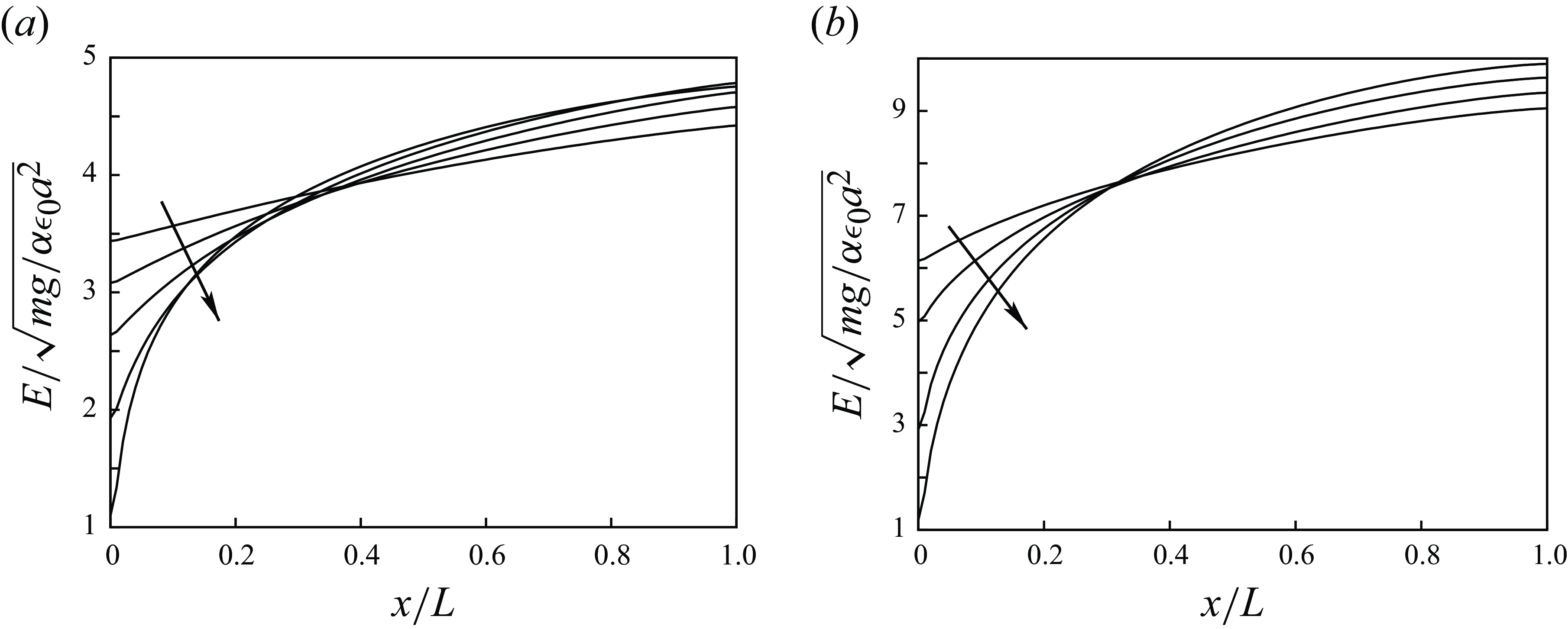
Figure 4. Distribution of the dimensionless electric field for (a) $V=4$
,
$V=4$
, $N=4$
, 6, 8, 10, 10.5, and (b)
$N=4$
, 6, 8, 10, 10.5, and (b) $V=8$
,
$V=8$
, $N=25$
, 37, 43, 44, with
$N=25$
, 37, 43, 44, with $N$
increasing as indicated by the arrows.
$N$
increasing as indicated by the arrows.
3. Particle inertia
3.1. Kinetic equation
The analysis of the previous section relies on the assumption that the inertia of the particles in negligible in their streaming between collisions; i.e. that $t_{coll} \gg t_s$
with
$t_{coll} \gg t_s$
with $t_{coll}=\lambda /v_c$
and
$t_{coll}=\lambda /v_c$
and $t_s=m/c_f$
. Using the coarse estimations in that section for the characteristic values of the variables involved, we find
$t_s=m/c_f$
. Using the coarse estimations in that section for the characteristic values of the variables involved, we find $\lambda =L/(N a^2)$
and
$\lambda =L/(N a^2)$
and $v_c=q_c E_c/c_f=\epsilon _0 a^2 (V/L)^2/c_f$
, so the condition
$v_c=q_c E_c/c_f=\epsilon _0 a^2 (V/L)^2/c_f$
, so the condition $t_{coll} \gg t_s$
amounts to
$t_{coll} \gg t_s$
amounts to $V^2 N \ll c_f^2 L^3/(\epsilon _0 m a^4)$
. If this condition is not satisfied, then the inertia of the particles must be taken into account, and the full distribution function
$V^2 N \ll c_f^2 L^3/(\epsilon _0 m a^4)$
. If this condition is not satisfied, then the inertia of the particles must be taken into account, and the full distribution function $f({\boldsymbol{v}}, q, {\boldsymbol{E}}, {\boldsymbol{x}}, t)$
must be used. The limit
$f({\boldsymbol{v}}, q, {\boldsymbol{E}}, {\boldsymbol{x}}, t)$
must be used. The limit $t_{coll} \ll t_s$
is discussed in this section.
$t_{coll} \ll t_s$
is discussed in this section.
The distribution function satisfies the Boltzmann equation
 \begin{equation} \frac {\partial f}{\partial t} + {\boldsymbol{\nabla }}_x {\boldsymbol\cdot} \left ( {{\boldsymbol{v}} f} \right ) + {\boldsymbol{\nabla }}_v {\boldsymbol\cdot} \left ( {{\boldsymbol{a}} f} \right ) = {\mathcal C} \quad \mbox{with} \quad {\boldsymbol{a}} = \frac {1}{m} \left [ {m {\boldsymbol{g}} + q {\boldsymbol{E}} - c_f({\boldsymbol{v}} - {\boldsymbol{v}}_g)}\right ] , \end{equation}
where ${\boldsymbol{\nabla }}_x {\boldsymbol\cdot} (\bullet )$
and
${\boldsymbol{\nabla }}_x {\boldsymbol\cdot} (\bullet )$
and ${\boldsymbol{\nabla }}_v {\boldsymbol\cdot} (\bullet )$
are the divergence operators in the
${\boldsymbol{\nabla }}_v {\boldsymbol\cdot} (\bullet )$
are the divergence operators in the $\boldsymbol{x}$
and
$\boldsymbol{x}$
and $\boldsymbol{v}$
spaces. The expression of the collision term on the right-hand side of (3.1) can be written by analogy with a gas of rigid spheres, but taking into account the redistribution of charge in the collisions and the condition that the charge of the particles does not affect the redistribution of momentum and energy; cf. the discussion of these issues in § 1.2. As before, the collision term can be split into depleting and replenishing collisions,
$\boldsymbol{v}$
spaces. The expression of the collision term on the right-hand side of (3.1) can be written by analogy with a gas of rigid spheres, but taking into account the redistribution of charge in the collisions and the condition that the charge of the particles does not affect the redistribution of momentum and energy; cf. the discussion of these issues in § 1.2. As before, the collision term can be split into depleting and replenishing collisions, ${\mathcal C} = {\mathcal C}^- + {\mathcal C}^+$
. The expressions of each part are (see e.g. Vincenti & Krueger Reference Vincenti and Krueger1965 for details)
${\mathcal C} = {\mathcal C}^- + {\mathcal C}^+$
. The expressions of each part are (see e.g. Vincenti & Krueger Reference Vincenti and Krueger1965 for details)
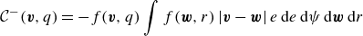 \begin{equation} {\mathcal C}^-({\boldsymbol{v}}, q) =-f({\boldsymbol{v}},q) \int {f({\boldsymbol{w}},r)\, |{\boldsymbol{v}} - {\boldsymbol{w}}|\, e \, \textrm {d} e \, \textrm {d} \psi \, \textrm {d} {\boldsymbol{w}} \, \textrm {d} r} \end{equation}
and
 \begin{equation} {\mathcal C}^+({\boldsymbol{v}}, q) = \int {f({\boldsymbol{v}}',q')\, f({\boldsymbol{w}}',r')\, \delta \left ( {\frac {q'+r'}{2} + q_{_E} - q} \right ) |{\boldsymbol{v}} - {\boldsymbol{w}}|\, e \, \textrm {d} e \, \textrm {d} \psi \, \textrm {d} {\boldsymbol{w}} \, \textrm {d} q' \, \textrm {d} r'} , \end{equation}
where, again to simplify the notation, only the first two arguments of the distribution function are indicated explicitly.
In (3.2), for depleting collisions, a particle with velocity $\boldsymbol{v}$
and charge
$\boldsymbol{v}$
and charge $q$
collides with a particle of velocity
$q$
collides with a particle of velocity $\boldsymbol{w}$
and charge
$\boldsymbol{w}$
and charge $r$
, generating two particles with velocities
$r$
, generating two particles with velocities ${\boldsymbol{v}}'$
and
${\boldsymbol{v}}'$
and ${\boldsymbol{w}}'$
and charges
${\boldsymbol{w}}'$
and charges $(q+r)/2-q_{_E}$
and
$(q+r)/2-q_{_E}$
and $(q+r)/2+q_{_E}$
, respectively, where
$(q+r)/2+q_{_E}$
, respectively, where $q_{_E}=\gamma \epsilon _0 a^2 E_{lc}$
, with
$q_{_E}=\gamma \epsilon _0 a^2 E_{lc}$
, with $E_{lc}$
the projection of the electric field in the direction of the line of centres, which is oriented now from the centre of the particle with velocity
$E_{lc}$
the projection of the electric field in the direction of the line of centres, which is oriented now from the centre of the particle with velocity $\boldsymbol{v}$
to the centre of the particle with velocity
$\boldsymbol{v}$
to the centre of the particle with velocity $\boldsymbol{w}$
, so
$\boldsymbol{w}$
, so $E_{lc}$
may be positive or negative. Here,
$E_{lc}$
may be positive or negative. Here, $e$
is the impact parameter sketched in figure 1, which ranges from 0 to
$e$
is the impact parameter sketched in figure 1, which ranges from 0 to $2 a$
, but the direction of the relative velocity
$2 a$
, but the direction of the relative velocity ${\boldsymbol{v}} - {\boldsymbol{w}}$
need not coincide now with that of the electric field. For each direction of
${\boldsymbol{v}} - {\boldsymbol{w}}$
need not coincide now with that of the electric field. For each direction of ${\boldsymbol{v}} - {\boldsymbol{w}}$
,
${\boldsymbol{v}} - {\boldsymbol{w}}$
, $\psi$
is the angle around the line with this direction through the centre of the particle with velocity
$\psi$
is the angle around the line with this direction through the centre of the particle with velocity $\boldsymbol{v}$
, which defines the position of the point of contact of the two particles in their collision. This angle ranges from 0 to
$\boldsymbol{v}$
, which defines the position of the point of contact of the two particles in their collision. This angle ranges from 0 to $2 \unicode{x03C0}$
, and for convenience, it is taken to be zero when the point of contact is in the plane defined by the centre of this particle and the direction of the electric field. The integrals over
$2 \unicode{x03C0}$
, and for convenience, it is taken to be zero when the point of contact is in the plane defined by the centre of this particle and the direction of the electric field. The integrals over $\boldsymbol{w}$
and
$\boldsymbol{w}$
and $r$
extend from
$r$
extend from $-\infty$
to
$-\infty$
to $\infty$
. The value of
$\infty$
. The value of $E_{lc}$
in
$E_{lc}$
in $q_{_E}$
depends on
$q_{_E}$
depends on $e$
and
$e$
and $\psi$
for each direction of
$\psi$
for each direction of ${\boldsymbol{v}} - {\boldsymbol{w}}$
.
${\boldsymbol{v}} - {\boldsymbol{w}}$
.
The velocities ${\boldsymbol{v}}'$
and
${\boldsymbol{v}}'$
and ${\boldsymbol{w}}'$
with which the particles emerge from the collision are known functions of
${\boldsymbol{w}}'$
with which the particles emerge from the collision are known functions of $\boldsymbol{v}$
and
$\boldsymbol{v}$
and $\boldsymbol{w}$
,
$\boldsymbol{w}$
, $e$
and
$e$
and $\psi$
, determined by the conditions of conservation of momentum and energy in the impact of two rigid spheres.
$\psi$
, determined by the conditions of conservation of momentum and energy in the impact of two rigid spheres.
In (3.3), for replenishing collisions, the mechanical inverse collision of each depleting collision is considered. The collision of particles with velocities ${\boldsymbol{v}}'$
and
${\boldsymbol{v}}'$
and ${\boldsymbol{w}}'$
and the same values of
${\boldsymbol{w}}'$
and the same values of $e$
and
$e$
and $\psi$
as in the (direct) depleting collision restores the initial velocities
$\psi$
as in the (direct) depleting collision restores the initial velocities $\boldsymbol{v}$
and
$\boldsymbol{v}$
and $\boldsymbol{w}$
. The modulus of the relative velocity
$\boldsymbol{w}$
. The modulus of the relative velocity $|{\boldsymbol{v}}' - {\boldsymbol{w}}'|$
coincides with
$|{\boldsymbol{v}}' - {\boldsymbol{w}}'|$
coincides with $|{\boldsymbol{v}} - {\boldsymbol{w}}|$
, and the volume element
$|{\boldsymbol{v}} - {\boldsymbol{w}}|$
, and the volume element $\textrm {d} {\boldsymbol{v}}' \, \textrm {d} {\boldsymbol{w}}'$
in velocity space coincides with
$\textrm {d} {\boldsymbol{v}}' \, \textrm {d} {\boldsymbol{w}}'$
in velocity space coincides with $\textrm {d} {\boldsymbol{v}} \, \textrm {d} {\boldsymbol{w}}$
(see e.g. Vincenti & Krueger Reference Vincenti and Krueger1965). However, these considerations do not extend to the charges of the particles. The charges
$\textrm {d} {\boldsymbol{v}} \, \textrm {d} {\boldsymbol{w}}$
(see e.g. Vincenti & Krueger Reference Vincenti and Krueger1965). However, these considerations do not extend to the charges of the particles. The charges $q'$
and
$q'$
and $r'$
of the particles entering a replenishing collision need not coincide with the charges with which the particles emerged from the corresponding direct depleting collision. The only constraint, enforced by the
$r'$
of the particles entering a replenishing collision need not coincide with the charges with which the particles emerged from the corresponding direct depleting collision. The only constraint, enforced by the $\delta$
function in (3.3), is that the charge of the particle emerging from the replenishing collision with velocity
$\delta$
function in (3.3), is that the charge of the particle emerging from the replenishing collision with velocity $\boldsymbol{v}$
must be
$\boldsymbol{v}$
must be $q$
. The charge of the particle emerging with velocity
$q$
. The charge of the particle emerging with velocity $\boldsymbol{w}$
will be different from
$\boldsymbol{w}$
will be different from $r$
, in general.
$r$
, in general.
As can be verified taking advantage of the presence of the $\delta$
function to simplify (3.3), the integral
$\delta$
function to simplify (3.3), the integral $\int _{-\infty }^{\infty }{{\mathcal C} \, \textrm {d} q}$
coincides with the usual expression of the collision term for a gas of rigid neutral spheres, written in terms of the marginal velocity distribution function
$\int _{-\infty }^{\infty }{{\mathcal C} \, \textrm {d} q}$
coincides with the usual expression of the collision term for a gas of rigid neutral spheres, written in terms of the marginal velocity distribution function $f_{v({\boldsymbol{v}})}=\int _{-\infty }^{\infty }{f({\boldsymbol{v}},q) \, \textrm {d} q}$
; see Appendix A.
$f_{v({\boldsymbol{v}})}=\int _{-\infty }^{\infty }{f({\boldsymbol{v}},q) \, \textrm {d} q}$
; see Appendix A.
Contrary to the previous section, collisions are understood here in the strict sense of contacts between particles. They conserve the number of particles, the momentum, the kinetic energy and the charge. Therefore,
 \begin{equation} \int {{\mathcal C} \, \textrm {d} {\boldsymbol{v}} \, \textrm {d} q} = \int {{\boldsymbol{v}} {\mathcal C} \, \textrm {d} {\boldsymbol{v}} \, \textrm {d} q} = \int {\frac {|{\boldsymbol{v}}|^2}{2} {\mathcal C} \, \textrm {d} {\boldsymbol{v}} \, \textrm {d} q} = \int {q {\mathcal C} \, \textrm {d} {\boldsymbol{v}} \, \textrm {d} q} = 0 . \end{equation}
3.2. Equilibrium distribution function
No attempt is made here to directly solve (3.1). Instead, the equilibrium distribution function that solves ${\mathcal C}(f_{eq})=0$
for given values of the electric field and the conserved magnitudes
${\mathcal C}(f_{eq})=0$
for given values of the electric field and the conserved magnitudes
 \begin{equation} n = \int {f \, \textrm {d} {\boldsymbol{v}} \, \textrm {d} q} , \quad {\boldsymbol{p}} = \int {{\boldsymbol{v}} f \, \textrm {d} {\boldsymbol{v}} \, \textrm {d} q} , \quad U = \int {\frac {|{\boldsymbol{v}}|^2}{2} f \, \textrm {d} {\boldsymbol{v}} \, \textrm {d} q}, \quad \rho _e = \int {q f \, \textrm {d} {\boldsymbol{v}} \, \textrm {d} q} , \end{equation}
is computed approximately using a direct simulation Monte Carlo method; see e.g. Garcia (Reference Garcia1999).
In conditions of near equilibrium, the collision-conserved moments (3.5) vary only over distances and times that are large compared with the mean free path $\lambda =1/(4 \sqrt {2} \unicode{x03C0} n a^2)$
and the mean time between collisions
$\lambda =1/(4 \sqrt {2} \unicode{x03C0} n a^2)$
and the mean time between collisions $t_{coll}$
, respectively. The same is true of the electric field, which is induced by the slowly varying charge density
$t_{coll}$
, respectively. The same is true of the electric field, which is induced by the slowly varying charge density $\rho _e$
and the constant interelectrode voltage. Thus it suffices to consider a uniform electric field to compute the equilibrium distribution function.
$\rho _e$
and the constant interelectrode voltage. Thus it suffices to consider a uniform electric field to compute the equilibrium distribution function.
Note that by addressing the problem ${\mathcal C}(f_{eq})=0$
, we are leaving out the effects of gravity and viscous friction, which appear in the transport operator (the left-hand side of (3.1)) but not in the collision operator. The distribution
${\mathcal C}(f_{eq})=0$
, we are leaving out the effects of gravity and viscous friction, which appear in the transport operator (the left-hand side of (3.1)) but not in the collision operator. The distribution $f_{eq}$
pertains to the double limit
$f_{eq}$
pertains to the double limit ${ Kn}=\lambda /L \rightarrow 0$
and
${ Kn}=\lambda /L \rightarrow 0$
and $t_{coll}/t_s \rightarrow 0$
. The effects of the non-zero values of both parameters are taken care of by the transport operator in (3.1), not by the functional form of
$t_{coll}/t_s \rightarrow 0$
. The effects of the non-zero values of both parameters are taken care of by the transport operator in (3.1), not by the functional form of $f_{eq}$
.
$f_{eq}$
.
A square two-dimensional numerical domain of side $L_b \gg \lambda$
in the direction of the electric field and in a direction perpendicular to it suffices for these computations, though, of course, the motion of the simulated particles is three-dimensional. Conditions of periodicity are used, reinjecting the particles that cross a side of the domain with the same velocity through the opposite side. The charges and velocities of the particles are written in the form
$L_b \gg \lambda$
in the direction of the electric field and in a direction perpendicular to it suffices for these computations, though, of course, the motion of the simulated particles is three-dimensional. Conditions of periodicity are used, reinjecting the particles that cross a side of the domain with the same velocity through the opposite side. The charges and velocities of the particles are written in the form $q_j=\overline {q} + q_j'$
and
$q_j=\overline {q} + q_j'$
and ${\boldsymbol{v}}_j=\overline {{\boldsymbol{v}}} + {\boldsymbol{v}}_j'$
, with
${\boldsymbol{v}}_j=\overline {{\boldsymbol{v}}} + {\boldsymbol{v}}_j'$
, with $\overline {q}=\rho _e/n$
and
$\overline {q}=\rho _e/n$
and $\overline {{\boldsymbol{v}}}={\boldsymbol{p}}/n$
, which are conserved in the collisions. The effect of
$\overline {{\boldsymbol{v}}}={\boldsymbol{p}}/n$
, which are conserved in the collisions. The effect of $\overline {q}$
is to cause a uniform acceleration
$\overline {q}$
is to cause a uniform acceleration $\overline {q} {\boldsymbol{E}}$
to the system of particles, which is removed by imposing the condition
$\overline {q} {\boldsymbol{E}}$
to the system of particles, which is removed by imposing the condition $\overline {q}=0$
on the initial charges of the particles. Galilean invariance implies that the value of
$\overline {q}=0$
on the initial charges of the particles. Galilean invariance implies that the value of $\boldsymbol{p}$
, which is conserved, does not change the functional form of the distribution function. The presence of
$\boldsymbol{p}$
, which is conserved, does not change the functional form of the distribution function. The presence of $\boldsymbol{p}$
is removed by choosing initial velocities of particles with a zero mean value.
$\boldsymbol{p}$
is removed by choosing initial velocities of particles with a zero mean value.
Two more comments are in order. First, dimensional analysis shows that the width of the $q'$
distribution scales with
$q'$
distribution scales with $q_{_E}=\gamma \epsilon _0 a^2 E$
, where
$q_{_E}=\gamma \epsilon _0 a^2 E$
, where $E$
is the strength of the uniform field acting on the particles. Second, anticipating the results of the computations displayed in figure 5 below, a correlation exists between
$E$
is the strength of the uniform field acting on the particles. Second, anticipating the results of the computations displayed in figure 5 below, a correlation exists between $q'$
and the component
$q'$
and the component $u'$
of the particle velocity
$u'$
of the particle velocity ${\boldsymbol{v}}'$
in the direction of the electric field. This implies that particles with a positive
${\boldsymbol{v}}'$
in the direction of the electric field. This implies that particles with a positive $q'$
are more likely to move in the direction of the electric field, and particles with a negative
$q'$
are more likely to move in the direction of the electric field, and particles with a negative $q'$
in the opposite direction. Owing to this correlation, the electric field continuously does work on the system of particles. While this energy input keeps the particles in a real EPS cell suspended despite the damping effect of the viscous friction with the gas, it must be artificially removed from the statistically homogeneous system used in the computations, or else the velocities of the particles would continuously increase with time. This is prevented by adding the fictitious drag force
$q'$
in the opposite direction. Owing to this correlation, the electric field continuously does work on the system of particles. While this energy input keeps the particles in a real EPS cell suspended despite the damping effect of the viscous friction with the gas, it must be artificially removed from the statistically homogeneous system used in the computations, or else the velocities of the particles would continuously increase with time. This is prevented by adding the fictitious drag force $-m {\boldsymbol{v}}/\sigma$
, with
$-m {\boldsymbol{v}}/\sigma$
, with $\sigma$
constant, during the streaming of the particles between collisions. Once the system of particles settles to a statistically stationary state, the mean rate at which the electric field does work on a particle, of order
$\sigma$
constant, during the streaming of the particles between collisions. Once the system of particles settles to a statistically stationary state, the mean rate at which the electric field does work on a particle, of order $q_c' E u_c'$
, where
$q_c' E u_c'$
, where $q_c'=q_{_E}$
and
$q_c'=q_{_E}$
and $u_c'$
is the characteristic width of the
$u_c'$
is the characteristic width of the $u'$
distribution, must be balanced by the rate of energy removal, of order
$u'$
distribution, must be balanced by the rate of energy removal, of order $m u_c^{\prime ^2}/\sigma$
. This balance determines the characteristic width of the
$m u_c^{\prime ^2}/\sigma$
. This balance determines the characteristic width of the $u'$
distribution as
$u'$
distribution as $u_c' \sim \sigma q_{_E} E/m$
.
$u_c' \sim \sigma q_{_E} E/m$
.
The particles in the domain are grouped in superparticles. Each superparticle obeys the same equations as individual particles (see (3.6) below), but it counts for as many particles as it represents in computing averages. In the computations of this section, $10^5$
superparticles were used with 100 particles per superparticle, and
$10^5$
superparticles were used with 100 particles per superparticle, and $L_b/\lambda =1110$
.
$L_b/\lambda =1110$
.
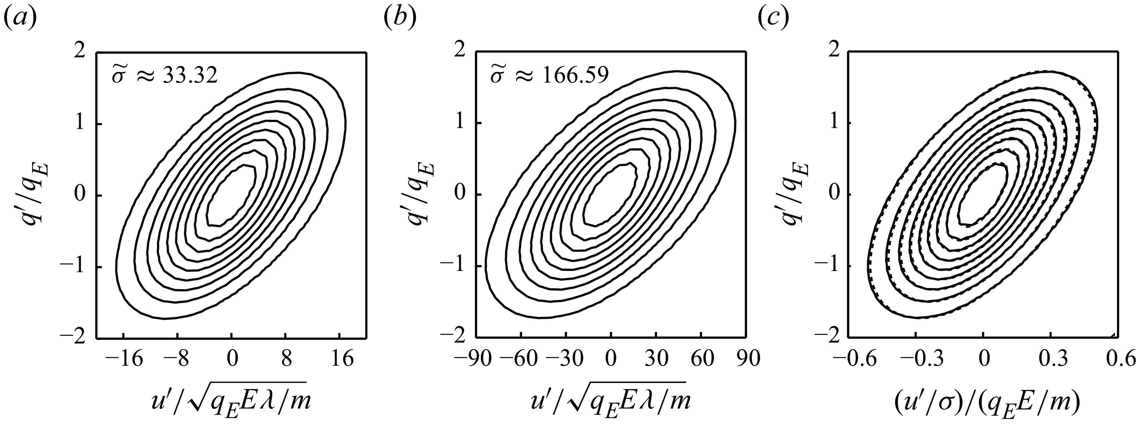
Figure 5. Nine equispaced contours of the joint equilibrium distribution function of the particle velocity component parallel to the electric field and the particle charge for ( $a$
)
$a$
) $\widetilde {\sigma } \approx 33.32$
and (
$\widetilde {\sigma } \approx 33.32$
and ( $b$
)
$b$
) $\widetilde {\sigma } \approx 166.59$
, showing the correlation between these variables. (
$\widetilde {\sigma } \approx 166.59$
, showing the correlation between these variables. ( $c$
) The results are superimposed (solid for
$c$
) The results are superimposed (solid for $\widetilde {\sigma } \approx 33.32$
, dashed for
$\widetilde {\sigma } \approx 33.32$
, dashed for $\widetilde {\sigma } \approx 166.59$
), showing that the width of the
$\widetilde {\sigma } \approx 166.59$
), showing that the width of the $u'$
distribution is proportional to
$u'$
distribution is proportional to $\sigma$
within the numerical error.
$\sigma$
within the numerical error.
The superparticles are marched in time. Each time step consists of streaming and collision phases. In the streaming phase, the three components of each particle ( $j$
) velocity and position are updated using a leapfrog scheme; i.e. adding to them
$j$
) velocity and position are updated using a leapfrog scheme; i.e. adding to them $\Delta {\boldsymbol{v}}_j$
and
$\Delta {\boldsymbol{v}}_j$
and $\Delta {\boldsymbol{x}}_j$
given by
$\Delta {\boldsymbol{x}}_j$
given by
 \begin{equation} m\, \Delta {\boldsymbol{v}}_j = \left ( {q_j {\boldsymbol{E}} - m {\boldsymbol{v}}_j/\sigma }\right ) \Delta t \quad \mbox{and} \quad \Delta {\boldsymbol{x}}_j = \left ( {{\boldsymbol{v}}_j + \Delta {\boldsymbol{v}}_j} \right ) \Delta t , \end{equation}
with $\Delta t$
chosen for the mean displacement of the superparticles in a time step to be of the order of their mean free path.
$\Delta t$
chosen for the mean displacement of the superparticles in a time step to be of the order of their mean free path.
In the collision phase, the domain is split into $N_{cell}^2$
equal cells of size comparable to the mean free path of the superparticles. A representative number of superparticle pairs is selected in each cell on the basis of the number of superparticles present in the cell and their relative velocities, but disregarding their positions (see Garcia Reference Garcia1999 for details). Collisions are assumed to occur between pairs of these superparticles, instantaneously changing their velocities and charges in accordance with the conditions of conservation of momentum, energy and charge in each collision, and assuming a random uniform distribution of the contact point on the particle surface.
$N_{cell}^2$
equal cells of size comparable to the mean free path of the superparticles. A representative number of superparticle pairs is selected in each cell on the basis of the number of superparticles present in the cell and their relative velocities, but disregarding their positions (see Garcia Reference Garcia1999 for details). Collisions are assumed to occur between pairs of these superparticles, instantaneously changing their velocities and charges in accordance with the conditions of conservation of momentum, energy and charge in each collision, and assuming a random uniform distribution of the contact point on the particle surface.
Histograms of the velocity and charge of the system of particles are computed by accumulating the velocities and charges of the particles over a large number of time steps, after the system has been left to evolve from an arbitrary initial state for a sufficiently long time for the initial conditions to be obliterated.
Scaling charges and velocities with $q_{_E}=\gamma \epsilon _0 a^2 E$
and
$q_{_E}=\gamma \epsilon _0 a^2 E$
and $v_{\lambda }=(q_{_E} E \lambda /m)^{1/2}$
, and the time with
$v_{\lambda }=(q_{_E} E \lambda /m)^{1/2}$
, and the time with $t_{\lambda }=\lambda /v_{\lambda }$
(which differs from the inverse of the mean collision frequency by a factor
$t_{\lambda }=\lambda /v_{\lambda }$
(which differs from the inverse of the mean collision frequency by a factor $2 \sqrt {2/\unicode{x03C0} }$
), the equilibrium solution depends only on
$2 \sqrt {2/\unicode{x03C0} }$
), the equilibrium solution depends only on $\widetilde {\sigma }=\sigma /t_{\lambda }$
, which is the ratio of the energy removal time to the mean time between particle collisions. This ratio has to be large for the energy removal not to inhibit the interaction between particles.
$\widetilde {\sigma }=\sigma /t_{\lambda }$
, which is the ratio of the energy removal time to the mean time between particle collisions. This ratio has to be large for the energy removal not to inhibit the interaction between particles.
As far as this condition is satisfied, numerical results for different values of $\widetilde {\sigma }$
show that, within the accuracy of the computations, the shape of the distribution function is independent of
$\widetilde {\sigma }$
show that, within the accuracy of the computations, the shape of the distribution function is independent of $\widetilde {\sigma }$
, while the width of the velocity distribution is proportional to it. This is in agreement with the previous estimation
$\widetilde {\sigma }$
, while the width of the velocity distribution is proportional to it. This is in agreement with the previous estimation $u_c' \sim \sigma q_{_E} E/m$
, which amounts to
$u_c' \sim \sigma q_{_E} E/m$
, which amounts to $(u_c'/v_{\lambda }) \sim \widetilde {\sigma }$
in dimensionless variables.
$(u_c'/v_{\lambda }) \sim \widetilde {\sigma }$
in dimensionless variables.
Figure 5 shows the joint equilibrium distribution function $f_{{eq}_{(u,q)}}(u,q)=\int {f_{eq} ({\boldsymbol{v}},q) \, \textrm {d} v \, \textrm {d} w}$
computed for two values of
$f_{{eq}_{(u,q)}}(u,q)=\int {f_{eq} ({\boldsymbol{v}},q) \, \textrm {d} v \, \textrm {d} w}$
computed for two values of $\widetilde {\sigma }$
. Here,
$\widetilde {\sigma }$
. Here, $v$
and
$v$
and $w$
are the velocity components perpendicular to the electric field. The two results are superimposed in figure 5(
$w$
are the velocity components perpendicular to the electric field. The two results are superimposed in figure 5( $c$
), revealing the universal form of the joint distribution when
$c$
), revealing the universal form of the joint distribution when $u'$
and
$u'$
and $q'$
are scaled with
$q'$
are scaled with $\widetilde {\sigma } v_{\lambda }$
and
$\widetilde {\sigma } v_{\lambda }$
and $q_{_E}$
, respectively. Results for other large values of
$q_{_E}$
, respectively. Results for other large values of $\widetilde {\sigma }$
support this conclusion.
$\widetilde {\sigma }$
support this conclusion.
No correlation exists between the charge and the velocity components perpendicular to the electric field (results not displayed). The variance is the same for the three velocity components, reflecting that collisions rapidly redistribute the energy supplied by the electric field.
The marginal velocity distribution $f_{eq_v}({\boldsymbol{v}})=\int _{-\infty }^{\infty }{f_{eq} \, \textrm {d} q}$
is a Maxwellian, in accordance with the fact that
$f_{eq_v}({\boldsymbol{v}})=\int _{-\infty }^{\infty }{f_{eq} \, \textrm {d} q}$
is a Maxwellian, in accordance with the fact that $\int _{-\infty }^{\infty }{{\mathcal C} \, \textrm {d} q}$
coincides with the collision term for a gas of neutral rigid spheres:
$\int _{-\infty }^{\infty }{{\mathcal C} \, \textrm {d} q}$
coincides with the collision term for a gas of neutral rigid spheres:
 \begin{equation} f_{eq_v}({\boldsymbol{v}}) = \frac {1}{n^{3/2} (2 k T/m)^{3/2}} \exp \left [ {-\frac {(u-\overline {u})^2 + (v-\overline {v})^2+(w-\overline {w})^2}{2 k T/m} }\right ] , \end{equation}
where $u$
,
$u$
, $v$
,
$v$
, $w$
are the Cartesian components of the particle velocity,
$w$
are the Cartesian components of the particle velocity, $\overline {u}$
,
$\overline {u}$
, $\overline {v}$
,
$\overline {v}$
, $\overline {w}$
are their mean values, which are zero in these computations, and the standard notation
$\overline {w}$
are their mean values, which are zero in these computations, and the standard notation $k T/m$
, with
$k T/m$
, with $T$
the granular temperature, is used for the variance of the velocity.
$T$
the granular temperature, is used for the variance of the velocity.
The marginal charge distribution $f_{{eq}_q}(q)=\int {f_{eq} \, \textrm {d} {\boldsymbol{v}}}$
is not a Maxwellian. It can be better fitted by
$f_{{eq}_q}(q)=\int {f_{eq} \, \textrm {d} {\boldsymbol{v}}}$
is not a Maxwellian. It can be better fitted by
 \begin{equation} f_{{eq}_q}(q)= A \, \exp \left [ {-0.55 \left ( \frac {q-\overline {q}}{\gamma \epsilon _0 a^2 E} \right )^2 - 0.075 \left ( \frac {q-\overline {q}}{\gamma \epsilon _0 a^2 E} \right )^4}\right ] , \end{equation}
with $\overline {q}=0$
in these computations.
$\overline {q}=0$
in these computations.
The joint distribution function $f_{{eq}_(u,q)}(u,q)$
is not a Maxwellian, but its shape is universal when the variables
$f_{{eq}_(u,q)}(u,q)$
is not a Maxwellian, but its shape is universal when the variables $u'=u-\overline {u}$
and
$u'=u-\overline {u}$
and $q'=q-\overline {q}$
are scaled with
$q'=q-\overline {q}$
are scaled with $\sqrt {k T/m}$
and
$\sqrt {k T/m}$
and $q_{_E}$
, respectively.
$q_{_E}$
, respectively.
3.3. Hydrodynamic equations
Multiplying the Boltzmann equation (3.1) by 1, $\boldsymbol{v}$
,
$\boldsymbol{v}$
, $|{\boldsymbol{v}}|^2/2$
or
$|{\boldsymbol{v}}|^2/2$
or $q$
, integrating over
$q$
, integrating over $\boldsymbol{v}$
and
$\boldsymbol{v}$
and $q$
, taking into account (3.4), and integrating by parts the contribution of the term
$q$
, taking into account (3.4), and integrating by parts the contribution of the term ${\boldsymbol{\nabla }}_v {\boldsymbol\cdot} ( {{\boldsymbol{a}} f} )$
of (3.1), we obtain the conservation budgets (see Appendix B)
${\boldsymbol{\nabla }}_v {\boldsymbol\cdot} ( {{\boldsymbol{a}} f} )$
of (3.1), we obtain the conservation budgets (see Appendix B)
 \begin{align} &\qquad\qquad\qquad\qquad\,\, \frac {\partial n}{\partial t} + {\boldsymbol{\nabla }} {\boldsymbol\cdot} {\boldsymbol{p}} = 0, \end{align}
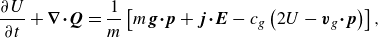 \begin{align} & \frac {\partial U}{\partial t} + {\boldsymbol{\nabla }} {\boldsymbol\cdot} {\boldsymbol{Q}} = \frac {1}{m} \left [ {m {\boldsymbol{g}} {\boldsymbol\cdot} {\boldsymbol{p}} + {\boldsymbol{j}} {\boldsymbol\cdot} {\boldsymbol{E}} - c_g \left ( {2 U - {\boldsymbol{v}}_g {\boldsymbol\cdot} {\boldsymbol{p}}}\right ) }\right ], \end{align}
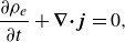 \begin{align} &\qquad\qquad\qquad\qquad \frac {\partial \rho _e}{\partial t} + {\boldsymbol{\nabla }} {\boldsymbol\cdot} {\boldsymbol{j}} = 0, \end{align}
where, in addition to the moments already defined in (3.5),
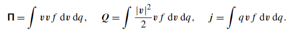
These moments of the distribution function can be computed approximately in conditions of near equilibrium when $f=f_{eq}$
at leading order in an expansion of the distribution function in powers of the Knudsen number
$f=f_{eq}$
at leading order in an expansion of the distribution function in powers of the Knudsen number ${ Kn} = \lambda /L \ll 1$
, where
${ Kn} = \lambda /L \ll 1$
, where $L$
is again the characteristic size of the suspension.
$L$
is again the characteristic size of the suspension.
The moments $U$
,
$U$
, ![]() and
and $\boldsymbol {Q}$
are the same as for a monoatomic gas, because the integrals over
$\boldsymbol {Q}$
are the same as for a monoatomic gas, because the integrals over $q$
can be done beforehand, and these moments depend only on the marginal velocity distribution
$q$
can be done beforehand, and these moments depend only on the marginal velocity distribution $f_{{eq}_v}({\boldsymbol{v}})$
. Thus
$f_{{eq}_v}({\boldsymbol{v}})$
. Thus
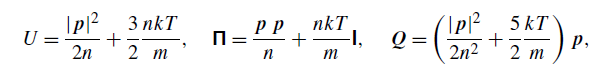
where $\boldsymbol{\mathsf{I}}$
is the unit tensor.
$\boldsymbol{\mathsf{I}}$
is the unit tensor.
The components of the current density $\boldsymbol{j}$
perpendicular to the electric field,
$\boldsymbol{j}$
perpendicular to the electric field, ${\boldsymbol{j}}_{\perp }$
say, can also be simply evaluated as
${\boldsymbol{j}}_{\perp }$
say, can also be simply evaluated as ${\boldsymbol{j}}_{\perp }=\rho _e {\boldsymbol{p}}_{\perp }/n$
, because the variables
${\boldsymbol{j}}_{\perp }=\rho _e {\boldsymbol{p}}_{\perp }/n$
, because the variables ${\boldsymbol{v}}_{\perp }$
and
${\boldsymbol{v}}_{\perp }$
and $q$
are statistically independent.
$q$
are statistically independent.
Finally, the component of $\boldsymbol{j}$
parallel to the electric field can be written as
$\boldsymbol{j}$
parallel to the electric field can be written as
 \begin{equation} j_{_{\parallel }}=\int {q v_{_{\parallel }} f \, \textrm {d} {\boldsymbol{v}} \, \textrm {d} q} = \frac {\rho _e p_{_{\parallel }}}{n} + \int {\left ( {q - \frac {\rho _e}{n} }\right ) \left ( {v_{_{\parallel }} - \frac {p_{_{\parallel }}}{n} }\right ) f \, \textrm {d} {\boldsymbol{v}} \, \textrm {d} q} , \end{equation}
where only the second term requires using the full distribution function computed approximately in the previous section. Since this function is known only numerically, the integral must also be evaluated numerically. The result is $0.45 \, n\, \sqrt {k T/m}\, \gamma \epsilon _0 a^2 E$
, where the universal shape of the joint distribution function has been used, and the factor 0.45 is known only to the accuracy of the previous computations.
$0.45 \, n\, \sqrt {k T/m}\, \gamma \epsilon _0 a^2 E$
, where the universal shape of the joint distribution function has been used, and the factor 0.45 is known only to the accuracy of the previous computations.
Carrying these results to (3.9)–(3.12), introducing the notation $\overline {{\boldsymbol{v}}}={\boldsymbol{p}}/n$
,
$\overline {{\boldsymbol{v}}}={\boldsymbol{p}}/n$
, $\overline {q}=\rho _e/n$
, and then suppressing the bars in
$\overline {q}=\rho _e/n$
, and then suppressing the bars in $\overline {{\boldsymbol{v}}}$
and
$\overline {{\boldsymbol{v}}}$
and $\overline {q}$
, which are no longer necessary, we obtain conservation equations analogous to the Euler equations for a monoatomic gas:
$\overline {q}$
, which are no longer necessary, we obtain conservation equations analogous to the Euler equations for a monoatomic gas:
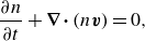 \begin{align} &\qquad\qquad\qquad\qquad\qquad\qquad\quad \frac {\partial n}{\partial t} + {\boldsymbol{\nabla }} {\boldsymbol\cdot} \left ( {n {\boldsymbol{v}}} \right ) = 0, \end{align}
 \begin{align} &\qquad\qquad \frac {\partial }{\partial t} \left ( {n {\boldsymbol{v}}}\right ) + {\boldsymbol{\nabla }} {\boldsymbol\cdot} \left ( {n {\boldsymbol{v}} {\boldsymbol{v}}}\right ) + {\boldsymbol{\nabla }} \frac {n k T}{m} = \frac {n}{m} [ {m {\boldsymbol{g}} + q {\boldsymbol{E}} - c_f ( {{\boldsymbol{v}} - {\boldsymbol{v}}_g}) }], \end{align}
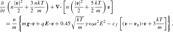 \begin{align} & \frac {\partial }{\partial t} \left ( {n \frac {|{\boldsymbol{v}}|^2}{2} + \frac {3}{2} \frac {n k T}{m} }\right ) + {\boldsymbol{\nabla }} {\boldsymbol\cdot} \left [ {n \left ( {\frac {|{\boldsymbol{v}}|^2}{2} + \frac {5}{2} \frac {k T}{m} }\right ) {\boldsymbol{v}}}\right ] \nonumber \\ & \quad = \frac {n}{m} \left \{ {m {\boldsymbol{g}} {\boldsymbol\cdot} {\boldsymbol{v}} + q {\boldsymbol{E}} {\boldsymbol\cdot} {\boldsymbol{v}} + 0.45 \, \sqrt {\frac {k T}{m}}\, \gamma \epsilon _0 a^2 E^2 - c_f \left [ {( {{\boldsymbol{v}} - {\boldsymbol{v}}_g} ) {\boldsymbol\cdot} {\boldsymbol{v}} + 3 \frac {k T}{m} }\right ] } \right \}, \end{align}
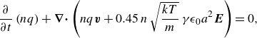 \begin{align} &\qquad\qquad\quad \frac {\partial }{\partial t} \left ( {n q} \right ) + {\boldsymbol{\nabla }} {\boldsymbol\cdot} \left ( {n q {\boldsymbol{v}} + 0.45 \, n\, \sqrt {\frac {k T}{m}}\, \gamma \epsilon _0 a^2 {\boldsymbol{E}}} \right ) = 0 , \end{align}
which must be supplemented with a Poisson equation for the electric potential,
 \begin{equation} \nabla ^2 \phi =-\frac {\rho _e}{\epsilon _0} , \end{equation}
and the Navier–Stokes equations for the gas. Leaving out compressibility effects, and taking into account the force that the particles exert on the gas, these equations read
 \begin{equation} {\boldsymbol{\nabla }} {\boldsymbol\cdot} {\boldsymbol{v}}_g=0 , \quad \frac {\partial {\boldsymbol{v}}_g}{\partial t} + {\boldsymbol{v}}_g {\boldsymbol\cdot} {\boldsymbol{\nabla }} {\boldsymbol{v}}_g =-{\boldsymbol{\nabla }} \frac {p_g}{\rho _g} + \mu _g\, \nabla ^2 {\boldsymbol{v}}_g + n c_f ( {{\boldsymbol{v}} - {\boldsymbol{v}}_g}) , \end{equation}
for a dilute suspension with very small solid volume fraction.
Equations (3.16)–(3.18) can be transformed much as the Euler equations for a gas. Both (3.17) and (3.18) can be rewritten in non-conservation form by subtracting from them the continuity equation (3.16) multiplied by $\boldsymbol{v}$
or
$\boldsymbol{v}$
or $|{\boldsymbol{v}}|^2/2+(3/2) k T/m$
. The following form of the energy equation is obtained by subtracting from the non-conservative form of (3.18) the dot product of
$|{\boldsymbol{v}}|^2/2+(3/2) k T/m$
. The following form of the energy equation is obtained by subtracting from the non-conservative form of (3.18) the dot product of $\boldsymbol{v}$
with the non-conservation form of (3.17):
$\boldsymbol{v}$
with the non-conservation form of (3.17):
 \begin{equation} n\, \frac {\partial }{\partial t} \left ( {\frac {3}{2} \frac {k T}{m} }\right ) + n {\boldsymbol{v}} {\boldsymbol\cdot} {\boldsymbol{\nabla }} \left ( {\frac {3}{2} \frac {k T}{m} }\right ) + \frac {n k T}{m}\, {\boldsymbol{\nabla }} {\boldsymbol\cdot} {\boldsymbol{v}} = \frac {n}{m} \left ( {0.45 \, \sqrt {\frac {k T}{m}}\, \gamma \epsilon _0 a^2 E^2 - 3 c_f \frac {k T}{m} }\right ) . \end{equation}
This equation will be used in the next subsection instead of (3.18).
3.4. Simplification of the particle phase equations when viscous friction dominates
The effect of the viscous friction of the particles with the gas is small during the streaming of the particles between consecutive collisions because the viscous adaptation time is large compared with the mean time between collisions, $t_s \gg t_{coll}$
. However, viscous friction may play an important role in longer time scales. In an EPS cell,
$t_s \gg t_{coll}$
. However, viscous friction may play an important role in longer time scales. In an EPS cell, $t_s$
is typically short compared with the transit time of a typical particle across the cell,
$t_s$
is typically short compared with the transit time of a typical particle across the cell, $t_r=L/v_c$
.
$t_r=L/v_c$
.
In these conditions, assuming that the macroscopic state of the suspension changes in times of order $t_r$
or larger, the first two terms on the left-hand side of the momentum equation (3.17) are of order
$t_r$
or larger, the first two terms on the left-hand side of the momentum equation (3.17) are of order $n_c v_c/t_r=n_c v_c^2/L$
. Now, the velocity of the gas,
$n_c v_c/t_r=n_c v_c^2/L$
. Now, the velocity of the gas, ${\boldsymbol{v}}_g$
in the right-hand side of this equation, is at most of the order of the mean velocity of the particles, because the motion of the gas is due to the drag of the particles. Therefore the last term on the right-hand side of (3.17) (the friction force) is of order
${\boldsymbol{v}}_g$
in the right-hand side of this equation, is at most of the order of the mean velocity of the particles, because the motion of the gas is due to the drag of the particles. Therefore the last term on the right-hand side of (3.17) (the friction force) is of order $(n_c/m) c_f v_c=n_c v_c/t_s$
, which is much larger than the first two terms terms on the left-hand side. The other two terms on the right-hand side (the gravity and electric forces) are at least of the order of the friction force, because this force is a consequence of the motion of the particles, which is induced by the gravity and the electric forces in an EPS cell. In summary, (3.17) reduces to
$(n_c/m) c_f v_c=n_c v_c/t_s$
, which is much larger than the first two terms terms on the left-hand side. The other two terms on the right-hand side (the gravity and electric forces) are at least of the order of the friction force, because this force is a consequence of the motion of the particles, which is induced by the gravity and the electric forces in an EPS cell. In summary, (3.17) reduces to
 \begin{equation} {\boldsymbol{\nabla }} \frac {n k T}{m} = \frac {n}{m} \left [ {m {\boldsymbol{g}} + q {\boldsymbol{E}} - c_f({\boldsymbol{v}}-{\boldsymbol{v}}_g)} \right ] \end{equation}
in first approximation for $t_r \gg t_s$
. This equation differs from the balance of forces found in the previous section for inertialess particles only in the pressure-like force on its left-hand side.
$t_r \gg t_s$
. This equation differs from the balance of forces found in the previous section for inertialess particles only in the pressure-like force on its left-hand side.
The ratio of the order-of-magnitude of each of the three terms on the left-hand side of (3.22) to the order-of-magnitude of the last term on the right-hand side is $t_s/t_r \ll 1$
, so (3.22) reduces to
$t_s/t_r \ll 1$
, so (3.22) reduces to
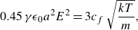 \begin{equation} 0.45 \, \gamma \epsilon _0 a^2 E^2 = 3 c_f\, \sqrt {\frac {k T}{m}} , \end{equation}
which is a local balance between the energy supplied to the suspension by the electric field and the energy lost by viscous friction with the gas.
Summarising, (3.16)–(3.19) simplify to
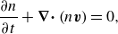 \begin{align} &\qquad\qquad\qquad\quad \frac {\partial n}{\partial t} + {\boldsymbol{\nabla }} {\boldsymbol\cdot} \left ( {n {\boldsymbol{v}}} \right ) = 0, \end{align}
 \begin{align} &\qquad\,\, {\boldsymbol{\nabla }} \frac {n k T}{m} = \frac {n}{m} [ {m {\boldsymbol{g}} + q {\boldsymbol{E}} - c_f ({\boldsymbol{v}} - {\boldsymbol{v}}_g) }], \end{align}
 \begin{align} &\qquad\qquad\,\,\, 0.45 \, \gamma \epsilon _0 a^2 E^2 = 3 c_f\, \sqrt {\frac {k T}{m}}, \end{align}
 \begin{align} & \frac {\partial }{\partial t} (n q) + {\boldsymbol{\nabla }} {\boldsymbol\cdot} \left ( {n q {\boldsymbol{v}} + 0.45 \, n\, \sqrt {\frac {k T}{m}}\, \gamma \epsilon _0 a^2 {\boldsymbol{E}}} \right ) = 0, \end{align}
when $t_{coll} \ll t_s \ll t_r$
.
$t_{coll} \ll t_s \ll t_r$
.
Equation (3.28) can be further simplified to
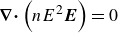 \begin{equation} {\boldsymbol{\nabla }} {\boldsymbol\cdot} \left ( {n E^2 {\boldsymbol{E}}} \right ) = 0 \end{equation}
by using (3.27) to eliminate $\sqrt {k T/m}$
and assuming that the suspension is sufficiently close to neutrality (
$\sqrt {k T/m}$
and assuming that the suspension is sufficiently close to neutrality ( $q/(\gamma \epsilon _0 a^2 E) \ll 1$
) to leave out the first two terms of (3.28).
$q/(\gamma \epsilon _0 a^2 E) \ll 1$
) to leave out the first two terms of (3.28).
4. Summary and future work
The dynamics of dilute suspensions of small, bipolarly charged particles in a gas has been analysed for particles of high electrical conductivity in two conditions of interest.
The inertia of the particles can be neglected when the mean time between particle collisions, $t_{coll}$
, is large compared with the viscous adaptation time
$t_{coll}$
, is large compared with the viscous adaptation time $t_s$
required for the particles to attain their terminal velocity under the action of electrical, gravity and viscous drag forces. The suspension approaches a continuum regime when the mean free path of the particles becomes small compared with the suspension size, which in an EPS cell occurs for values of the interelectrode voltage that are large compared with the minimum voltage required to electrically lift the particles, and values of the number of particles per unit electrode area nearing the maximum possible for the applied voltage.
$t_s$
required for the particles to attain their terminal velocity under the action of electrical, gravity and viscous drag forces. The suspension approaches a continuum regime when the mean free path of the particles becomes small compared with the suspension size, which in an EPS cell occurs for values of the interelectrode voltage that are large compared with the minimum voltage required to electrically lift the particles, and values of the number of particles per unit electrode area nearing the maximum possible for the applied voltage.
The inertia of the particles plays an important role in the opposite limit when $t_{coll} \ll t_s$
. The equilibrium distribution function in the continuum regime has been computed approximately in this case, and hydrodynamic equations analogous to the Euler equations for a monoatomic gas have been derived for the local number density of particles, their mean momentum and energy, and their mean charge, which are the magnitudes conserved in collisions. These equations simplify when the viscous adaptation time is small compared with the transit time of a particle across the suspension.
$t_{coll} \ll t_s$
. The equilibrium distribution function in the continuum regime has been computed approximately in this case, and hydrodynamic equations analogous to the Euler equations for a monoatomic gas have been derived for the local number density of particles, their mean momentum and energy, and their mean charge, which are the magnitudes conserved in collisions. These equations simplify when the viscous adaptation time is small compared with the transit time of a particle across the suspension.
Some limitations and future extensions of the work are briefly summarised.
The volume fraction of the particle phase, $\Phi =({4}/{3}) \unicode{x03C0} a^3 n \sim (a/L)/(\lambda /L)$
, has been assumed to be small, despite the small value of
$\Phi =({4}/{3}) \unicode{x03C0} a^3 n \sim (a/L)/(\lambda /L)$
, has been assumed to be small, despite the small value of $\lambda /L$
in the continuum regime. This is appropriate for dilute suspensions of small particles. An extension to account for non-zero values of
$\lambda /L$
in the continuum regime. This is appropriate for dilute suspensions of small particles. An extension to account for non-zero values of $\Phi$
would be desirable. This would require accounting for effects of the particles on the motion of the gas beyond the Stokes drag in (3.21), and probably also a modified kinetic equation for the distribution function.
$\Phi$
would be desirable. This would require accounting for effects of the particles on the motion of the gas beyond the Stokes drag in (3.21), and probably also a modified kinetic equation for the distribution function.
The electrical conductivity of the particles has been assumed to be sufficiently high for the transfer of charge in collisions to be effectively instantaneous. This is appropriate for metallic particles free from an oxide cover. A finite electrical conductivity introduces an electric relaxation time to characterise this process. This time is to be compared with the duration of particle contacts, which depends on the elastic properties of the particles and the electrodes. The problem for values of this time ratio of order unity has been tackled in Zhebelev (Reference Zhebelev1991, Reference Zhebelev1993) and Higuera (Reference Higuera2023) for inertialess particles using an effective conductivity model, and the analysis can be extended to account for the particle inertia. More complex mechanisms of contact charging (Matsusaka & Masuda Reference Matsusaka and Masuda2003; Laurentie, Traoré & Dascalescu Reference Laurentie, Traoré and Dascalescu2013) are needed to describe suspensions of less conducting or insulating materials of interest for other applications.
Inelastic collisions have not been taken into account. These collisions increase the energy dissipation rate above that due to viscous friction of the particles with the gas, which amounts to decreasing the dissipation time $t_s$
. Strongly inelastic collisions are incompatible with a condition of the type
$t_s$
. Strongly inelastic collisions are incompatible with a condition of the type $t_{coll}/t_s \ll 1$
, though they can be immediately accommodated in the analysis of § 2 for
$t_{coll}/t_s \ll 1$
, though they can be immediately accommodated in the analysis of § 2 for $t_{coll}/t_s$
large. Mildly inelastic collisions, leading to a dissipation rate of the same order as viscous friction, can be expected to fit into an extended form of the analysis in § 3 for small values of this time ratio.
$t_{coll}/t_s$
large. Mildly inelastic collisions, leading to a dissipation rate of the same order as viscous friction, can be expected to fit into an extended form of the analysis in § 3 for small values of this time ratio.
Funding
This work was supported by grants PID2020–115730GB-C22 and PID2023–150329NB-C22 funded by MCIN/AEI/10.13039, and by ERDF A way of making Europe.
Declaration of interests
The author reports no conflict of interest.
Appendix A. Collision operator for the marginal distribution function
The term ${\mathcal C}^-$
in (3.2) is just
${\mathcal C}^-$
in (3.2) is just
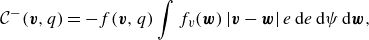 \begin{equation} {\mathcal C}^-({\boldsymbol{v}},q) =-f({\boldsymbol{v}},q) \int {f_v({\boldsymbol{w}})\, |{\boldsymbol{v}}-{\boldsymbol{w}}|\, e \, \textrm {d} e \, \textrm {d} \psi \, \textrm {d} {\boldsymbol{w}}} , \end{equation}
so on integrating over $q$
,
$q$
,
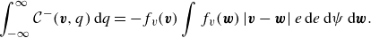 \begin{equation} \int _{-\infty }^{\infty }{{\mathcal C}^-({\boldsymbol{v}},q) \, \textrm {d} q} = -f_v({\boldsymbol{v}}) \int {f_v({\boldsymbol{w}})\, |{\boldsymbol{v}} - {\boldsymbol{w}}|\, e \, \textrm {d} e \, \textrm {d} \psi \, \textrm {d} {\boldsymbol{w}}} . \end{equation}
As for ${\mathcal C}^+$
, disposing of the
${\mathcal C}^+$
, disposing of the $\delta$
function in (3.3), we have
$\delta$
function in (3.3), we have
 \begin{equation} \int _{-\infty }^{\infty }{{\mathcal C}^+({\boldsymbol{v}},q) \, \textrm {d} q} = \int {f \left ( {{\boldsymbol{v}}', q-q_{_E} - \frac {r'}{2} }\right ) f({\boldsymbol{w}}',r')\, |{\boldsymbol{v}} - {\boldsymbol{w}}|\, e \, \textrm {d} e \, \textrm {d} \psi \, \textrm {d} {\boldsymbol{w}} \, \textrm {d} r' \, \textrm {d} q } , \end{equation}
which with the change of variables $\widetilde {q}=q-q_{_E}-r'/2$
,
$\widetilde {q}=q-q_{_E}-r'/2$
, $\widetilde {r}'=r'$
, becomes
$\widetilde {r}'=r'$
, becomes
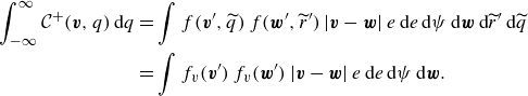 \begin{align} \int _{-\infty }^{\infty }{{\mathcal C}^+({\boldsymbol{v}},q) \, \textrm {d} q} & = \int {f({\boldsymbol{v}}',\widetilde {q})\, f({\boldsymbol{w}}',\widetilde {r}')\, |{\boldsymbol{v}}-{\boldsymbol{w}}|\, e \, \textrm {d} e \, \textrm {d} \psi \, \textrm {d} {\boldsymbol{w}} \, \textrm {d} \widetilde {r}' \, \textrm {d} \widetilde {q}} \nonumber \\ &= \int {f_v({\boldsymbol{v}}')\, f_v({\boldsymbol{w}}')\, |{\boldsymbol{v}}-{\boldsymbol{w}}|\, e \, \textrm {d} e \, \textrm {d} \psi \, \textrm {d} {\boldsymbol{w}}} . \end{align}
In summary, $\int _{-\infty }^{\infty }{ [{\mathcal C}^-({\boldsymbol{v}},q) + {\mathcal C}^+({\boldsymbol{v}},q) ] \, \textrm {d} q}$
coincides with the collision term for a gas of rigid neutral spheres, written in terms of the marginal distribution function
$\int _{-\infty }^{\infty }{ [{\mathcal C}^-({\boldsymbol{v}},q) + {\mathcal C}^+({\boldsymbol{v}},q) ] \, \textrm {d} q}$
coincides with the collision term for a gas of rigid neutral spheres, written in terms of the marginal distribution function $f_v({\boldsymbol{v}})=\int _{-\infty }^{\infty }{f({\boldsymbol{v}},q) \, \textrm {d} q}$
.
$f_v({\boldsymbol{v}})=\int _{-\infty }^{\infty }{f({\boldsymbol{v}},q) \, \textrm {d} q}$
.
Appendix B. Equations for conserved moments
Multiplying (3.1) by $1$
,
$1$
, $\boldsymbol{v}$
,
$\boldsymbol{v}$
, $|{\boldsymbol{v}}|^2/2$
or
$|{\boldsymbol{v}}|^2/2$
or $q$
, and integrating over
$q$
, and integrating over $\boldsymbol{v}$
and
$\boldsymbol{v}$
and $q$
as mentioned in the text, we have
$q$
as mentioned in the text, we have
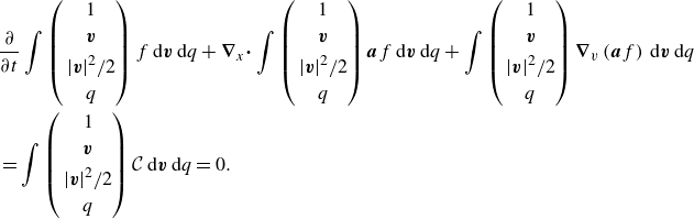 \begin{align} & \frac {\partial }{\partial t} \int { \left ( \begin{gathered} 1 \\ {\boldsymbol{v}} \\ |{\boldsymbol{v}}|^2/2 \\ q \end{gathered} \right ) f \, \textrm {d} {\boldsymbol{v}} \, \textrm {d} q} + {\boldsymbol{\nabla }}_x {\boldsymbol\cdot} \int { \left ( \begin{gathered} 1 \\ {\boldsymbol{v}} \\ |{\boldsymbol{v}}|^2/2 \\ q \end{gathered} \right ) {\boldsymbol{a}} f \, \textrm {d} {\boldsymbol{v}} \, \textrm {d} q} + \int { \left ( \begin{gathered} 1 \\ {\boldsymbol{v}} \\ |{\boldsymbol{v}}|^2/2 \\ q \end{gathered} \right ) {\boldsymbol{\nabla }}_v \left ( {{\boldsymbol{a}} f} \right ) \, \textrm {d} {\boldsymbol{v}} \, \textrm {d} q} \nonumber \\ & = \int { \left ( \begin{gathered} 1 \\ {\boldsymbol{v}} \\ |{\boldsymbol{v}}|^2/2 \\ q \end{gathered} \right ) {\mathcal C} \, \textrm {d} {\boldsymbol{v}} \, \textrm {d} q} = 0 . \end{align}
The last term on the left-hand side can be rewritten as
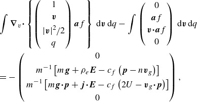 \begin{align} & \int {{\boldsymbol{\nabla }}_v {\boldsymbol\cdot} \left \{ { \left ( \begin{gathered} 1 \\ {\boldsymbol{v}} \\ |{\boldsymbol{v}}|^2/2 \\ q \end{gathered} \right ) {\boldsymbol{a}} f }\right \} \, \textrm {d} {\boldsymbol{v}} \, \textrm {d} q} - \int { \left ( \begin{gathered} 0 \\ {\boldsymbol{a}} f \\ {\boldsymbol{v}} {\boldsymbol\cdot} {\boldsymbol{a}} f \\ 0 \end{gathered} \right ) \, \textrm {d} {\boldsymbol{v}} \, \textrm {d} q} \nonumber \\ & = -\left ( \begin{gathered} 0 \\ m^{-1} \left [ m {\boldsymbol{g}} + \rho _e {\boldsymbol{E}} - c_f \left ( {{\boldsymbol{p}} - n {\boldsymbol{v}}_g} \right ) \right ] \\ m^{-1} \left [ m {\boldsymbol{g}} {\boldsymbol\cdot} {\boldsymbol{p}} + {\boldsymbol{j}} {\boldsymbol\cdot} {\boldsymbol{E}} - c_f \left ( {2 U - {\boldsymbol{v}}_g {\boldsymbol\cdot} {\boldsymbol{p}}} \right ) \right ] \\ 0 \end{gathered} \right ) , \end{align}
where the first term is zero, and use has been made of ${\boldsymbol{a}}=m^{-1} [ m {\boldsymbol{g}} + q {\boldsymbol{E}} - c_f({\boldsymbol{v}}-{\boldsymbol{v}}_g) ]$
in (3.1), the definitions of
${\boldsymbol{a}}=m^{-1} [ m {\boldsymbol{g}} + q {\boldsymbol{E}} - c_f({\boldsymbol{v}}-{\boldsymbol{v}}_g) ]$
in (3.1), the definitions of $n$
,
$n$
, $\boldsymbol{p}$
,
$\boldsymbol{p}$
, $U$
and
$U$
and $\rho _e$
in (3.5), and
$\rho _e$
in (3.5), and $\boldsymbol{j}$
in (3.13), to evaluate the integrals in the second term.
$\boldsymbol{j}$
in (3.13), to evaluate the integrals in the second term.
Equations (3.9)–(3.12) are just (B1) with the definitions of the moments in (3.5) and (3.13) used in the first two terms, the results (B2) moved to the right-hand sides, and the subscript $x$
in
$x$
in ${\boldsymbol{\nabla }}_x$
removed.
${\boldsymbol{\nabla }}_x$
removed.


 Open access