


1. Introduction
Particle-laden multiphase flows have long been, and actively remain, a critical area of study due to their broad application in various natural and industrial processes. These flows are essential for understanding applications such as sediment transport in rivers (Mercier et al. Reference Mercier, Wang, Péméja, Ern and Ardekani2020; Seyed-Ahmadi & Wachs Reference Seyed-Ahmadi and Wachs2021), polluant dispersion in oceans (Rahmani et al. Reference Rahmani, Gupta and Jofre2022, Reference Rahmani, Banaei, Brandt and Martinez2023), fluidised beds in chemical engineering (Dupuy, Ansart & Simonin Reference Dupuy, Ansart and Simonin2024; Hardy, Fede & Simonin Reference Hardy, Fede and Simonin2024) and bubbly flows in mechanical engineering (Chaparian & Frigaard Reference Chaparian and Frigaard2021; Bonnefis et al. Reference Bonnefis, Sierra-Ausin, Fabre and Magnaudet2024). The study of flows around rotating bluff bodies, including spheres, cylinders and other non-spherical particles, is essential for understanding the dynamics of these multiphase flows. It is well-established that the flow past a fixed bluff body, beyond a critical Reynolds number, leads to asymmetrical vortex shedding behind the body. These vortex-induced fluctuations are a primary cause of flow-induced vibration and fatigue, which, in extreme cases, may result in structural failure. Assigning rotation to the bluff body significantly modifies the flow dynamics compared with fixed bodies, potentially eliminating or reducing vortex shedding and the associated oscillations (Rashidi, Hayatdavoodi & Esfahani Reference Rashidi, Hayatdavoodi and Esfahani2016). These insights are critical for addressing various natural and engineering challenges, such as optimising the performance of drilling pipes (Chen et al. Reference Chen, Rheem, Lin and Li2020). Furthermore, the rotational dynamics of freely settling particles play a key role in determining path instability of individual particles (Gai & Wachs Reference Gai and Wachs2024), while also influencing the microstructure and collective behaviour of particle suspensions in inertial flow (Seyed-Ahmadi & Wachs Reference Seyed-Ahmadi and Wachs2019; Goyal et al. Reference Goyal, Gai, Cheng, Cunha, Zhu and Wachs2024) and turbulent boundary layers (Baker & Coletti Reference Baker and Coletti2021). Although extensive research has been conducted on flow past spheres and cylinders, flow interactions with rotating angular particles are less understood. Unlike their streamlined counterparts, angular particles with sharp edges and corners exhibit distinct flow characteristics, particularly in vortex generation and wake instability. This study seeks to address this gap by providing deeper insights into the complex flow interactions with a transversely rotating angular isometric polyhedron, uncovering the unique dynamics and behaviours that emerge from these interactions. In the following, we review the current understanding of flow past transversely rotating objects, such as spheres and cylinders, to provide context and clarify our motivation for focusing on the more complex and intriguing behaviour of rotating angular particles.
The dynamics of a flow around a rotating sphere has long attracted research interest and has been extensively studied, largely due to the simple geometry of the sphere. In both natural and industrial applications, transverse rotation is far more common than streamwise rotation in most practical scenarios, making it a key focus in the literature (Torobin & Gauvin Reference Torobin and Gauvin1959). A uniform flow past a transversely rotating sphere gives rise to a transverse hydrodynamic force known as the Magnus effect, which causes a deflection in the flight path of a freely moving sphere. Rubinow & Keller (Reference Rubinow and Keller1961) were among the first to investigate these dynamics in Stokes flow, discovering that while the drag force remains independent of rotation and equal to the Stokes drag, the lift coefficient is proportional to the rotation rate, expressed as $C_l = 2\Omega$
, where
$C_l = 2\Omega$
, where $\Omega$
is the dimensionless rotation rate of the particle, using the free stream velocity and the sphere radius as reference scales. For inertial flow, Tsuji, Morikawa & Mizuno (Reference Tsuji, Morikawa and Mizuno1985) assumed a proportional relationship between lift and rotation, and proposed the correlation
$\Omega$
is the dimensionless rotation rate of the particle, using the free stream velocity and the sphere radius as reference scales. For inertial flow, Tsuji, Morikawa & Mizuno (Reference Tsuji, Morikawa and Mizuno1985) assumed a proportional relationship between lift and rotation, and proposed the correlation $C_l = (0.4\pm 0.1)\Omega$
for Reynolds numbers
$C_l = (0.4\pm 0.1)\Omega$
for Reynolds numbers $550 \leqslant {{R}e} \leqslant 1600$
and rotation rates
$550 \leqslant {{R}e} \leqslant 1600$
and rotation rates $\Omega \lt 0.7$
. Oesterlé & Dinh (Reference Oesterlé and Dinh1998) focused on lower Reynolds numbers,
$\Omega \lt 0.7$
. Oesterlé & Dinh (Reference Oesterlé and Dinh1998) focused on lower Reynolds numbers, $10 \leqslant {{R}e} \leqslant 140$
, and higher rotation rates,
$10 \leqslant {{R}e} \leqslant 140$
, and higher rotation rates, $1 \leqslant \Omega \leqslant 6$
, providing a correlation based on experimental data:
$1 \leqslant \Omega \leqslant 6$
, providing a correlation based on experimental data: $C_l = 0.45 + (2\Omega - 0.45)\exp (-0.075\Omega ^{0.4}{{R}e}^{0.7})$
. For moderate flow inertia (
$C_l = 0.45 + (2\Omega - 0.45)\exp (-0.075\Omega ^{0.4}{{R}e}^{0.7})$
. For moderate flow inertia ( $100 \leqslant {{R}e} \leqslant 500$
) and low rotation rates (
$100 \leqslant {{R}e} \leqslant 500$
) and low rotation rates ( $0.16 \leqslant \Omega \leqslant 0.5$
), Niazmand & Renksizbulut (Reference Niazmand and Renksizbulut2003) introduced another empirical correlation:
$0.16 \leqslant \Omega \leqslant 0.5$
), Niazmand & Renksizbulut (Reference Niazmand and Renksizbulut2003) introduced another empirical correlation: $C_l = 0.11 (1 + \Omega )^{3.6}$
. Unless otherwise specified,
$C_l = 0.11 (1 + \Omega )^{3.6}$
. Unless otherwise specified, ${R}e$
is computed using the free stream velocity and the sphere diameter for a meaningful comparison with published work. Further efforts have been made to generalise these empirical correlations over broader ranges of
${R}e$
is computed using the free stream velocity and the sphere diameter for a meaningful comparison with published work. Further efforts have been made to generalise these empirical correlations over broader ranges of ${R}e$
and
${R}e$
and $\Omega$
, with these advancements thoroughly summarised by Shi & Rzehak (Reference Shi and Rzehak2019). In general, the lift coefficient
$\Omega$
, with these advancements thoroughly summarised by Shi & Rzehak (Reference Shi and Rzehak2019). In general, the lift coefficient $C_l$
of a rotating sphere increases with
$C_l$
of a rotating sphere increases with $\Omega$
, but decreases with
$\Omega$
, but decreases with ${R}e$
. A bifurcation effect occurs around
${R}e$
. A bifurcation effect occurs around ${{R}e} = 200$
, which significantly influences the Magnus effect, particularly at low rotation rates (Shi & Rzehak Reference Shi and Rzehak2019).
${{R}e} = 200$
, which significantly influences the Magnus effect, particularly at low rotation rates (Shi & Rzehak Reference Shi and Rzehak2019).
With regards to wake instability, the flow at low inertia past a rotating sphere undergoes a series of regime transitions, characterised by changes in wake vortical structures, as ${R}e$
and
${R}e$
and $\Omega$
vary. For low
$\Omega$
vary. For low ${R}e$
at
${R}e$
at $\Omega \lt 0.5$
, the rotation can trigger a vortex shedding, with the shedding frequency
$\Omega \lt 0.5$
, the rotation can trigger a vortex shedding, with the shedding frequency $\mathcal{S}\textit{tr}$
modulated by
$\mathcal{S}\textit{tr}$
modulated by $\Omega$
(Best Reference Best1998; Niazmand & Renksizbulut Reference Niazmand and Renksizbulut2003). As the rotation rate increases, the mean length of the recirculation region progressively shrinks and shifts towards the high-pressure side, eventually disappearing entirely for
$\Omega$
(Best Reference Best1998; Niazmand & Renksizbulut Reference Niazmand and Renksizbulut2003). As the rotation rate increases, the mean length of the recirculation region progressively shrinks and shifts towards the high-pressure side, eventually disappearing entirely for $\Omega \gt 0.5$
. The fluid passing through the low-pressure region is dragged along the lee side of the sphere until it encounters fluid moving downstream over the high-pressure side, where it is peeled off the sphere surface to form a shear layer. At
$\Omega \gt 0.5$
. The fluid passing through the low-pressure region is dragged along the lee side of the sphere until it encounters fluid moving downstream over the high-pressure side, where it is peeled off the sphere surface to form a shear layer. At ${{R}e} = 250$
, vortex suppression occurs around
${{R}e} = 250$
, vortex suppression occurs around $\Omega = 0.3$
, where two steady vortical threads form in the wake region, and the flow remains steady (Giacobello, Ooi & Balachandar Reference Giacobello, Ooi and Balachandar2009). At a higher Reynolds number of
$\Omega = 0.3$
, where two steady vortical threads form in the wake region, and the flow remains steady (Giacobello, Ooi & Balachandar Reference Giacobello, Ooi and Balachandar2009). At a higher Reynolds number of ${{R}e} = 300$
, periodic vortex shedding reappears for
${{R}e} = 300$
, periodic vortex shedding reappears for $\Omega \geqslant 0.8$
, where the vortical threads in the near-wake tilt and evolve into a one-sided hairpin structure, driven by oblique Kelvin–Helmholtz instability (Giacobello et al. Reference Giacobello, Ooi and Balachandar2009; Poon et al. Reference Poon, OOi, Giacobello and Cohen2013). With further increase of the flow inertia beyond
$\Omega \geqslant 0.8$
, where the vortical threads in the near-wake tilt and evolve into a one-sided hairpin structure, driven by oblique Kelvin–Helmholtz instability (Giacobello et al. Reference Giacobello, Ooi and Balachandar2009; Poon et al. Reference Poon, OOi, Giacobello and Cohen2013). With further increase of the flow inertia beyond ${{R}e} \geqslant 500$
and
${{R}e} \geqslant 500$
and $\Omega \geqslant 0.8$
, the flow structures transition into the shear layer stable foci regime before becoming fully chaotic (Poon et al. Reference Poon, Ooi, Giacobello, Iaccarino and Chung2014). A second type of studies investigates the turbulent regimes,
$\Omega \geqslant 0.8$
, the flow structures transition into the shear layer stable foci regime before becoming fully chaotic (Poon et al. Reference Poon, Ooi, Giacobello, Iaccarino and Chung2014). A second type of studies investigates the turbulent regimes, ${{R}e} \geqslant 10^4$
, particularly focusing on the inverse Magnus effect (Kim et al. Reference Kim, Choi, Park and Yoo2014). Recent experiments have revealed varying Magnus effects, in the intermediate range of
${{R}e} \geqslant 10^4$
, particularly focusing on the inverse Magnus effect (Kim et al. Reference Kim, Choi, Park and Yoo2014). Recent experiments have revealed varying Magnus effects, in the intermediate range of $10^3 \leqslant {{R}e} \leqslant 10^4$
(Sareen, Hourigan & Thompson Reference Sareen, Hourigan and Thompson2024). At extremely high rotation rates,
$10^3 \leqslant {{R}e} \leqslant 10^4$
(Sareen, Hourigan & Thompson Reference Sareen, Hourigan and Thompson2024). At extremely high rotation rates, $\Omega \geqslant 4$
, upstream vortex shedding has been observed, characterised by the formation of multiple small-scale vortex filaments (De & Sarkar Reference De and Sarkar2023). Additionally, many studies have explored wake instability in the flow past a rotating sphere through linear and weakly nonlinear analyses, shedding light on the competitive interactions of global modes in pattern formation (Citro et al. Reference Citro, Tchoufag, Fabre, Giannetti and Luchini2016; Jiménez-González et al. Reference Jiménez-González, Manglano-Villamarín and Coenen2019; Sierra-Ausín et al. Reference Sierra-Ausín, Lorite-Díez, Jiménez-González, Citro and Fabre2022). These analyses provide deep insights into the mechanisms driving flow transitions and vortex dynamics in various regimes of transversely rotating spheres.
$\Omega \geqslant 4$
, upstream vortex shedding has been observed, characterised by the formation of multiple small-scale vortex filaments (De & Sarkar Reference De and Sarkar2023). Additionally, many studies have explored wake instability in the flow past a rotating sphere through linear and weakly nonlinear analyses, shedding light on the competitive interactions of global modes in pattern formation (Citro et al. Reference Citro, Tchoufag, Fabre, Giannetti and Luchini2016; Jiménez-González et al. Reference Jiménez-González, Manglano-Villamarín and Coenen2019; Sierra-Ausín et al. Reference Sierra-Ausín, Lorite-Díez, Jiménez-González, Citro and Fabre2022). These analyses provide deep insights into the mechanisms driving flow transitions and vortex dynamics in various regimes of transversely rotating spheres.
In addition to spheres, bluff bodies with non-spherical geometries, particularly cylinder-like shapes, have also been the focus of extensive research. In two-dimensional (2-D) simulations, vortex suppression has been observed in rotating circular and square cylinders (Kang, Choi & Lee Reference Kang, Choi and Lee1999; Khan et al. Reference Khan, Anwer, Khan and Hasan2021; Karimi-Zindashti & Kurç Reference Karimi-Zindashti and Kurç2024). A distinctive feature of flow past rotating square cylinders is the development of near-field wakes along the upper or lower (depending on the rotation direction) side of the square, which evolve independently from the main wake and differ significantly from the case of circular cylinders or spheres (Karimi-Zindashti & Kurç Reference Karimi-Zindashti and Kurç2024). Yang et al. (Reference Yang, Wang, Guo and Zhang2023) explored three-dimensional flow dynamics around a rotating circular cylinder of finite length with the axis perpendicular to the flow at ${{R}e} \lt 500$
and
${{R}e} \lt 500$
and $\Omega \leqslant 2$
. For a cylinder with aspect ratio of
$\Omega \leqslant 2$
. For a cylinder with aspect ratio of $1$
and
$1$
and $\Omega \leqslant 0.3$
, the wake pattern is similar to that of a fixed cylinder, though with a new linearly unstable mode competing to dominate the wake saturation state. At
$\Omega \leqslant 0.3$
, the wake pattern is similar to that of a fixed cylinder, though with a new linearly unstable mode competing to dominate the wake saturation state. At $\Omega \geqslant 0.9$
, a new low-frequency wake structure emerges, characterised by stronger oscillations. Yang et al. (Reference Yang, Wang, Guo and Zhang2023) also identified new flow modes and conducted global stability analyses, finding that the dynamics of a rotating short cylinder with an aspect ratio slightly greater than
$\Omega \geqslant 0.9$
, a new low-frequency wake structure emerges, characterised by stronger oscillations. Yang et al. (Reference Yang, Wang, Guo and Zhang2023) also identified new flow modes and conducted global stability analyses, finding that the dynamics of a rotating short cylinder with an aspect ratio slightly greater than $1$
resembles that of a rotating sphere. As the aspect ratio increases, the flow becomes increasingly unstable at
$1$
resembles that of a rotating sphere. As the aspect ratio increases, the flow becomes increasingly unstable at $\Omega \lt 0.6$
, emphasising the significant influence of particle shape on wake instability.
$\Omega \lt 0.6$
, emphasising the significant influence of particle shape on wake instability.
In recent years, there has been a growing interest in the flow interactions with angular particles, driven by their unique behaviours in fluid flow and critical roles in chemical and mechanical engineering processes (Seyed-Ahmadi & Wachs Reference Seyed-Ahmadi and Wachs2019; Angle, Rau & Byron Reference Angle, Rau and Byron2024; Marquardt, Hafen & Krause Reference Marquardt, Hafen and Krause2024; Wang et al. Reference Wang, Xiao, Liu, Sun, Liu, Liang, Zhang and Zhang2024). A exemplary case is the use of soft hydro-gel cubes, which swell in response to changes in pressure, temperature and pH of the flow environment. These hydrogel cubes present an innovative approach for detecting fluctuations in brain fluids, offering significant potential for non-invasive in vivo diagnostics (Tang et al. Reference Tang2024). As a result, understanding the intricate flow interactions with angular particles, such as cubes, is becoming increasingly vital for advancing technological applications. Numerous studies have examined the interactions between flows and fixed angular particles. Saha (Reference Saha2004) conducted body-fitted numerical simulations of the laminar flow past a fixed cube at $20 \leqslant {{R}e}_{{edge}} \leqslant 300$
, with
$20 \leqslant {{R}e}_{{edge}} \leqslant 300$
, with ${{R}e}_{{edge}}$
the Reynolds number based on cube edge length. They found that the transition sequence and flow structures are comparable to those observed around a fixed sphere, although with different critical Reynolds numbers of regime transition. Later, Klotz et al. (Reference Klotz, Goujon-Durand, Rokicki and Wesfreid2014) carried out an extensive experimental investigation of the wake behind a fixed cube for
${{R}e}_{{edge}}$
the Reynolds number based on cube edge length. They found that the transition sequence and flow structures are comparable to those observed around a fixed sphere, although with different critical Reynolds numbers of regime transition. Later, Klotz et al. (Reference Klotz, Goujon-Durand, Rokicki and Wesfreid2014) carried out an extensive experimental investigation of the wake behind a fixed cube for $20 \leqslant {{R}e}_{{edge}} \leqslant 400$
, using particle image velocimetry and laser-induced fluorescence. Their study identified two bifurcations indicating the transition from steady to unsteady flow regimes. More recently, Meng et al. (Reference Meng, An, Cheng and Kimiaei2021) performed high-fidelity body-fitted numerical simulation of flows past a fixed cube at
$20 \leqslant {{R}e}_{{edge}} \leqslant 400$
, using particle image velocimetry and laser-induced fluorescence. Their study identified two bifurcations indicating the transition from steady to unsteady flow regimes. More recently, Meng et al. (Reference Meng, An, Cheng and Kimiaei2021) performed high-fidelity body-fitted numerical simulation of flows past a fixed cube at $1 \leqslant {{R}e}_{{edge}} \leqslant 400$
, providing accurate critical Reynolds numbers for regime transition further confirmed by weakly nonlinear instability analysis. In our previous works, we systematically explored the flow behaviour past a fixed Platonic polyhedron at
$1 \leqslant {{R}e}_{{edge}} \leqslant 400$
, providing accurate critical Reynolds numbers for regime transition further confirmed by weakly nonlinear instability analysis. In our previous works, we systematically explored the flow behaviour past a fixed Platonic polyhedron at $100 \leqslant {{R}e} \leqslant 500$
(Gai & Wachs Reference Gai and Wachs2023a
,Reference Gai and Wachs
c
,Reference Gai and Wachs
d
). Our findings revealed that both the angularity and the angular position of the particle significantly influence wake structures in steady and unsteady regimes. In the steady regime, the generation of streamwise vortex pairs is determined by the inclined particle front faces. The shape of the particle significantly influences the recirculation region, resulting in distinct vortex shedding patterns. These dynamic wake features, in turn, modify the hydrodynamic force and torque acting on the particle (Gai & Wachs Reference Gai and Wachs2023b
). In terms of moving angular particles, new regimes, such as the helical settling regime, emerge for freely settling Platonic polyhedrons in quiescent flow, driven by enhanced rotation of particles with high angularity (Rahmani & Wachs Reference Rahmani and Wachs2014; Seyed-Ahmadi & Wachs Reference Seyed-Ahmadi and Wachs2019; Gai & Wachs Reference Gai and Wachs2024). Daghooghi & Borazjani (Reference Daghooghi and Borazjani2018) demonstrated that irregular-shaped particles, which have more extended surface areas or mass distributions farther from their centres, experience amplified hydrodynamic forces. They further showed that modelling such particles using simple regular shapes can lead to underestimation of both stress and viscosity, emphasising the critical role of realistic particle shape in accurately predicting suspension rheology.
$100 \leqslant {{R}e} \leqslant 500$
(Gai & Wachs Reference Gai and Wachs2023a
,Reference Gai and Wachs
c
,Reference Gai and Wachs
d
). Our findings revealed that both the angularity and the angular position of the particle significantly influence wake structures in steady and unsteady regimes. In the steady regime, the generation of streamwise vortex pairs is determined by the inclined particle front faces. The shape of the particle significantly influences the recirculation region, resulting in distinct vortex shedding patterns. These dynamic wake features, in turn, modify the hydrodynamic force and torque acting on the particle (Gai & Wachs Reference Gai and Wachs2023b
). In terms of moving angular particles, new regimes, such as the helical settling regime, emerge for freely settling Platonic polyhedrons in quiescent flow, driven by enhanced rotation of particles with high angularity (Rahmani & Wachs Reference Rahmani and Wachs2014; Seyed-Ahmadi & Wachs Reference Seyed-Ahmadi and Wachs2019; Gai & Wachs Reference Gai and Wachs2024). Daghooghi & Borazjani (Reference Daghooghi and Borazjani2018) demonstrated that irregular-shaped particles, which have more extended surface areas or mass distributions farther from their centres, experience amplified hydrodynamic forces. They further showed that modelling such particles using simple regular shapes can lead to underestimation of both stress and viscosity, emphasising the critical role of realistic particle shape in accurately predicting suspension rheology.
Despite these valuable insights gained for fixed and freely moving angular particles, our understanding of the flow dynamics around rotating angular particles remains limited. To bridge this gap, we investigate the flow past a transversely rotating cube at moderate Reynolds numbers and extend the analysis to other isometric angular polyhedrons, including the tetrahedron and octahedron, to gain a more comprehensive understanding. This study aims to address four key questions: (i) what drives vortex generation on the surface of a rotating angular particle?; (ii) what mechanisms control the suppression and reemergence of vortex shedding behind angular particles?; (iii) how do rotational symmetry and particle geometry affect wake stability and regime transitions?; and (iv) what impact does particle angularity have on hydrodynamic forces?
The rest of the paper is organised as follows. Section 2 outlines the numerical methods, defines the dimensionless parameters and details the simulation set-up. Section 3 presents the numerical validation of the flow past a rotating sphere. In § 4, we provide a detailed analysis of the flow dynamics around a rotating cube, with a focus on regime transitions, on vortex generation and merging, and on the influence of rotation on wake instability, hydrodynamic forces and vortex shedding frequency. Building on the insights gained from the rotating cube, § 5 expands the investigation to other angular particles, specifically tetrahedrons and octahedrons, with different numbers of rotational symmetry folds. Finally, § 6 presents the key conclusions and potential perspectives for future research.
2. Numerical method, dimensionless numbers and numerical set-up
The distributed Lagrange multiplier/fictitious domain (DLM/FD) method simulates a rigid body immersed in the fluid by introducing a fictitious domain $P$
. Within this domain, rigid-body constraints are enforced to ensure it behaves like a rigid particle. Throughout this paper, dimensional quantities are indicated with a superscript
$P$
. Within this domain, rigid-body constraints are enforced to ensure it behaves like a rigid particle. Throughout this paper, dimensional quantities are indicated with a superscript $^*$
, while non-dimensional quantities are presented without any superscript. We consider a large cubic computational domain
$^*$
, while non-dimensional quantities are presented without any superscript. We consider a large cubic computational domain $\mathcal{D}$
with boundary
$\mathcal{D}$
with boundary $\Gamma$
, containing a solid sub-domain
$\Gamma$
, containing a solid sub-domain $P$
, which represents a rigid body immersed in a Newtonian fluid with constant density
$P$
, which represents a rigid body immersed in a Newtonian fluid with constant density $\rho _f^*$
and viscosity
$\rho _f^*$
and viscosity $\mu _f^*$
. To clearly distinguish between the fluid and solid regions, the fluid sub-domain is defined as
$\mu _f^*$
. To clearly distinguish between the fluid and solid regions, the fluid sub-domain is defined as $\mathcal{D} \setminus P$
, ensuring no overlap between the fluid and solid domains, i.e.
$\mathcal{D} \setminus P$
, ensuring no overlap between the fluid and solid domains, i.e. $\mathcal{D} \setminus P \cap P = \emptyset$
. The DLM/FD method used in this study has been thoroughly discussed and validated in prior works (Glowinski et al. Reference Glowinski, Pan, Hesla and Joseph1999; Wachs Reference Wachs2009, Reference Wachs2011; Wachs et al. Reference Wachs, Hammouti, Vinay and Rahmani2015; Selçuk et al. Reference Selçuk, Ghigo, Popinet and Wachs2021). For the sake of brevity, we present only a brief overview of the governing equations for fluid motion and the coupled equations governing the motion of the particle–fluid mixture in Appendix A.
$\mathcal{D} \setminus P \cap P = \emptyset$
. The DLM/FD method used in this study has been thoroughly discussed and validated in prior works (Glowinski et al. Reference Glowinski, Pan, Hesla and Joseph1999; Wachs Reference Wachs2009, Reference Wachs2011; Wachs et al. Reference Wachs, Hammouti, Vinay and Rahmani2015; Selçuk et al. Reference Selçuk, Ghigo, Popinet and Wachs2021). For the sake of brevity, we present only a brief overview of the governing equations for fluid motion and the coupled equations governing the motion of the particle–fluid mixture in Appendix A.
2.1. Dimensionless numbers
The governing equations (A1)–(A2) can be non-dimensionalised using the following reference scales: the reference length $L_{ref}^* = D_{sph}^*$
, where
$L_{ref}^* = D_{sph}^*$
, where $D_{sph}^*$
is the diameter of the volume-equivalent sphere defined later; the reference velocity
$D_{sph}^*$
is the diameter of the volume-equivalent sphere defined later; the reference velocity $U_{ref}^* = U_0^*$
, corresponding to the incoming flow velocity; the reference time scale
$U_{ref}^* = U_0^*$
, corresponding to the incoming flow velocity; the reference time scale $L_{ref}^*/U_{ref}^*$
; the reference pressure
$L_{ref}^*/U_{ref}^*$
; the reference pressure $\rho _f^* U_{ref}^{*,2}$
and the reference moment of inertia tensor
$\rho _f^* U_{ref}^{*,2}$
and the reference moment of inertia tensor $\rho _s^* L_{ref}^{*,5}$
.
$\rho _s^* L_{ref}^{*,5}$
.
The key dimensionless quantities considered in this study are: (i) the particle Reynolds number ${R}e$
, the rotational rate
${R}e$
, the rotational rate $\Omega$
, the particle angularity
$\Omega$
, the particle angularity $\phi$
and rotational symmetry fold
$\phi$
and rotational symmetry fold $n_{\Omega }$
; and (ii) output parameters such as the lift coefficient
$n_{\Omega }$
; and (ii) output parameters such as the lift coefficient $C_l$
, the drag coefficient
$C_l$
, the drag coefficient $C_d$
, the rotation coefficient
$C_d$
, the rotation coefficient $C_{\Omega }$
, the vortex shedding frequency
$C_{\Omega }$
, the vortex shedding frequency $\mathcal{S}\textit{tr}$
and the dimensionless vorticity
$\mathcal{S}\textit{tr}$
and the dimensionless vorticity $\boldsymbol{\omega }$
, along with other relevant quantities.
$\boldsymbol{\omega }$
, along with other relevant quantities.
The particle Reynolds number ${R}e$
is defined as
${R}e$
is defined as
 \begin{equation} {{R}e} = \frac {\rho _f^* U_{ref}^*D_{sph}^*}{\mu _f^*}. \end{equation}
Since we consider different angular particles with the same volume, ${R}e$
is defined based on the diameter of a sphere with the same volume as the angular particle, referred to as the volume-equivalent sphere and computed by
${R}e$
is defined based on the diameter of a sphere with the same volume as the angular particle, referred to as the volume-equivalent sphere and computed by
 \begin{equation} D_{sph}^* = \left ( \frac {6}{\pi } V_{Particle}^* \right )^{1/3}, \end{equation}
where $V_{Particle}^*$
is the volume of the angular particle.
$V_{Particle}^*$
is the volume of the angular particle.
Particle sphericity, denoted by $\phi$
, quantifies how closely an angular particle resembles a perfect sphere. Specifically,
$\phi$
, quantifies how closely an angular particle resembles a perfect sphere. Specifically, $\phi$
is defined as the ratio of the surface area of the volume-equivalent sphere,
$\phi$
is defined as the ratio of the surface area of the volume-equivalent sphere, $S_{sph}^*$
, to the surface area of an angular particle,
$S_{sph}^*$
, to the surface area of an angular particle, $S_p^*$
, as given by the following equation:
$S_p^*$
, as given by the following equation:
 \begin{equation} \phi = \frac {S_{sph}^*}{S_p^*}. \end{equation}
The level of non-sphericity is inversely proportional to $\phi$
. When
$\phi$
. When $\phi$
is close to
$\phi$
is close to $1$
, the particle shape closely approximates a sphere. In the present study, non-sphericity is equivalent to angularity, and the level of angularity is inversely proportional to
$1$
, the particle shape closely approximates a sphere. In the present study, non-sphericity is equivalent to angularity, and the level of angularity is inversely proportional to $\phi$
. As expected, we have
$\phi$
. As expected, we have $\phi _{tetrahedron} \lt \phi _{cube} \lt \phi _{octahedron}$
.
$\phi _{tetrahedron} \lt \phi _{cube} \lt \phi _{octahedron}$
.
We define the dimensionless rotation rate as follows:
 \begin{equation} \boldsymbol{\Omega } = \frac {\boldsymbol{\Omega ^*} D_{sph}^*}{2U_{ref}^*}, \end{equation}
where $\boldsymbol{\Omega ^*}$
represents the rotation rate of the angular particle around the transverse direction, chosen here as the
$\boldsymbol{\Omega ^*}$
represents the rotation rate of the angular particle around the transverse direction, chosen here as the $z$
direction. During the rotation, the number of rotational symmetry folds
$z$
direction. During the rotation, the number of rotational symmetry folds $n_{\Omega }$
refers to the number of times an angular particle can be rotated by equal angles around the rotation axis and still appear identical to its original angular position.
$n_{\Omega }$
refers to the number of times an angular particle can be rotated by equal angles around the rotation axis and still appear identical to its original angular position.
The drag coefficient $C_d$
and the lift coefficients
$C_d$
and the lift coefficients $C_{l,y}$
and
$C_{l,y}$
and $C_{l,z}$
for a rotating particle are defined as follows:
$C_{l,z}$
for a rotating particle are defined as follows:
 \begin{equation} C_d = \frac {8F_x^*}{\pi \rho _f^*{U_{ref}^*}^{2}D_{sph}^{*,2}}, \quad C_{l,y} = \frac {8F_y^*}{\pi \rho _f^*{U_{ref}^*}^{2}D_{sph}^{*,2}}, \quad C_{l,z} = \frac {8F_z^*}{\pi \rho _f^*{U_{ref}^*}^{2}D_{sph}^{*,2}}, \end{equation}
where $\boldsymbol{F}^*$
denotes the hydrodynamic force exerted on the angular particle. Similarly, the torque coefficients are calculated as
$\boldsymbol{F}^*$
denotes the hydrodynamic force exerted on the angular particle. Similarly, the torque coefficients are calculated as
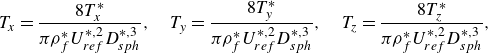 \begin{equation} T_x = \frac {8T_x^*}{\pi \rho _f^* U_{ref}^{*,2} D_{sph}^{*,3}}, \quad T_y = \frac {8T_y^*}{\pi \rho _f^* U_{ref}^{*,2} D_{sph}^{*,3}}, \quad T_z = \frac {8T_z^*}{\pi \rho _f^* U_{ref}^{*,2} D_{sph}^{*,3}}, \end{equation}
where $T_i^*$
represents the
$T_i^*$
represents the $i$
th component of the hydrodynamic torque
$i$
th component of the hydrodynamic torque $\boldsymbol{T^*}$
for
$\boldsymbol{T^*}$
for $i \in \{x, y, z\}$
. Please note that in the context of the DLM/FD method (Seyed-Ahmadi & Wachs Reference Seyed-Ahmadi and Wachs2020), the hydrodynamic force
$i \in \{x, y, z\}$
. Please note that in the context of the DLM/FD method (Seyed-Ahmadi & Wachs Reference Seyed-Ahmadi and Wachs2020), the hydrodynamic force $\boldsymbol{F}^*$
and torque
$\boldsymbol{F}^*$
and torque $\boldsymbol{T}^*$
are calculated using the integral of the Lagrange multipliers over
$\boldsymbol{T}^*$
are calculated using the integral of the Lagrange multipliers over $P$
, such that
$P$
, such that
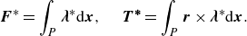 \begin{equation} {\boldsymbol{F}}^*= \int _{P} \boldsymbol{\lambda }^*{\rm d}\boldsymbol{x}, \,\quad \boldsymbol{T^*}= \int _{P} \boldsymbol{r}\times \boldsymbol{\lambda }^*{\rm d}\boldsymbol{x}. \end{equation}
Furthermore, the rotation coefficient $C_\Omega$
is introduced to quantify the relationship between the Magnus lift force and the rotation rate
$C_\Omega$
is introduced to quantify the relationship between the Magnus lift force and the rotation rate $\Omega ^*=||\boldsymbol{\Omega ^*}||$
. It is calculated as
$\Omega ^*=||\boldsymbol{\Omega ^*}||$
. It is calculated as
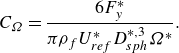 \begin{equation} C_{\Omega } = \frac {6F_y^*}{\pi \rho _f U_{ref}^* D_{sph}^{*,3}{\Omega ^*}}. \end{equation}
The Strouhal number characterises the oscillatory behaviour of the flow in the wake of the particle and is defined as
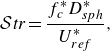 \begin{equation} \mathcal{S}\textit{tr} = \frac {f_c^* D_{sph}^*}{U_{ref}^*}, \end{equation}
By normalising $f_c^*$
with
$f_c^*$
with $U_{ref}^*/D_{sph}^*$
, which corresponds to the inverse of the advective time scale, the
$U_{ref}^*/D_{sph}^*$
, which corresponds to the inverse of the advective time scale, the $\mathcal{S}\textit{tr}$
captures the characteristic frequency of vortex shedding.
$\mathcal{S}\textit{tr}$
captures the characteristic frequency of vortex shedding.
To better visualise the wake structures, the dimensionless vorticity, which measures fluid rotation, is computed as follows:
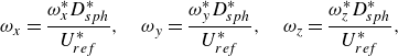 \begin{equation} \omega _x = \frac {\omega ^*_x D_{sph}^*}{U_{ref}^*}, \quad \omega _y = \frac {\omega ^*_y D_{sph}^*}{U_{ref}^*}, \quad \omega _z = \frac {\omega ^*_z D_{sph}^*}{U_{ref}^*}, \end{equation}
where $\omega ^*_x$
,
$\omega ^*_x$
, $\omega ^*_y$
and
$\omega ^*_y$
and $\omega ^*_z$
are the components of the vorticity in the
$\omega ^*_z$
are the components of the vorticity in the $x$
,
$x$
, $y$
and
$y$
and $z$
directions, respectively.
$z$
directions, respectively.
2.2. Numerical set-up
We present in figure 1 the cubic computational domain $\mathcal{D}$
selected to perform our numerical simulations. The cubic domain has an edge length of
$\mathcal{D}$
selected to perform our numerical simulations. The cubic domain has an edge length of $L_0=40$
and is filled with a Newtonian fluid. The angular particle is positioned at (
$L_0=40$
and is filled with a Newtonian fluid. The angular particle is positioned at ( $10$
,
$10$
, $20$
,
$20$
, $20$
), with a transversely rotating axis along the
$20$
), with a transversely rotating axis along the $z$
direction. Figure 1 shows the vortex structures identified by the isosurface of
$z$
direction. Figure 1 shows the vortex structures identified by the isosurface of $\lambda _2 = -1$
in the wake of a rotating cube with a four-fold rotational symmetry axis (hereafter referred to as RCF4). The negative value of the
$\lambda _2 = -1$
in the wake of a rotating cube with a four-fold rotational symmetry axis (hereafter referred to as RCF4). The negative value of the $\lambda _2$
-criterion identifies vortex cores as regions where local fluid rotation dominates over strain (Jeong & Hussain Reference Jeong and Hussain1995). The flow is depicted at
$\lambda _2$
-criterion identifies vortex cores as regions where local fluid rotation dominates over strain (Jeong & Hussain Reference Jeong and Hussain1995). The flow is depicted at ${{R}e} = 200$
and
${{R}e} = 200$
and $\Omega = 0.3$
, with the region of interest highlighted in a pink box. The size disparity between the particle and the computational domain is particularly noticeable. Figure 1 illustrates the octree grid within the three-dimensional computational domain, highlighting the advantages of adaptive mesh refinement in accurately simulating flow dynamics in a large domain that models a quasi unbounded domain. To enhance visualisation, two zoomed views are provided: an
$\Omega = 0.3$
, with the region of interest highlighted in a pink box. The size disparity between the particle and the computational domain is particularly noticeable. Figure 1 illustrates the octree grid within the three-dimensional computational domain, highlighting the advantages of adaptive mesh refinement in accurately simulating flow dynamics in a large domain that models a quasi unbounded domain. To enhance visualisation, two zoomed views are provided: an $x$
-
$x$
- $z$
cut-plane at
$z$
cut-plane at $y=19$
on the right-top panel of figure 1 and a side view of the
$y=19$
on the right-top panel of figure 1 and a side view of the $x$
-
$x$
- $y$
cut-plane at
$y$
cut-plane at $z=20$
on the right-bottom panel, which reveal the high mesh resolution near the surface of the cube as well as in the wake region loaded with vortex structures.
$z=20$
on the right-bottom panel, which reveal the high mesh resolution near the surface of the cube as well as in the wake region loaded with vortex structures.
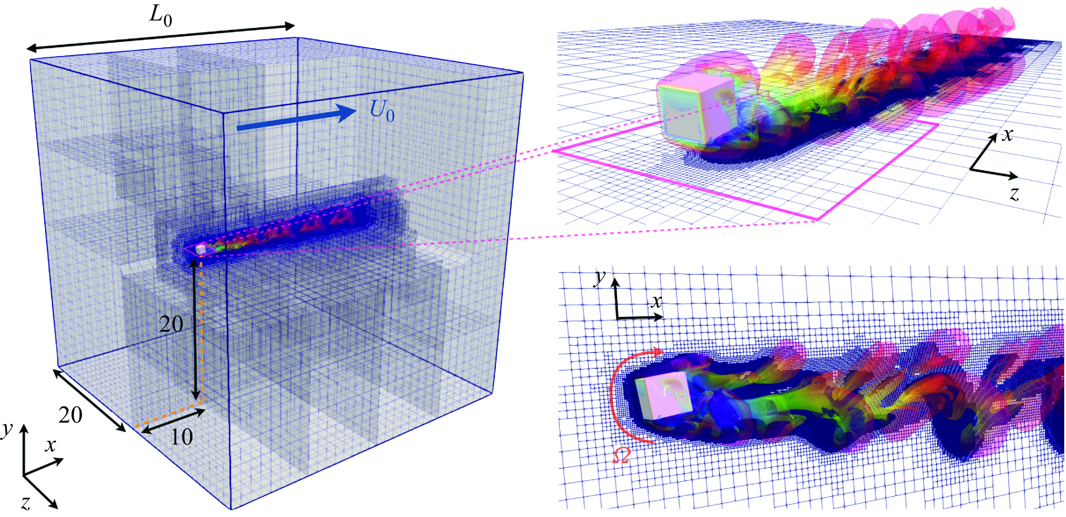
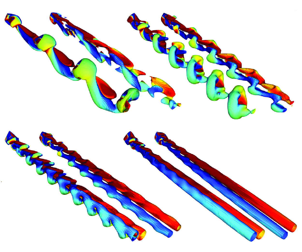
Figure 1. Computational domain and wake structures of the flow past a rotating cube at $\Omega =0.3$
and
$\Omega =0.3$
and ${{R}e}=200$
with a four-fold rotational symmetry axis (RCF4) aligned along the
${{R}e}=200$
with a four-fold rotational symmetry axis (RCF4) aligned along the $z$
-axis. Vortical structures, identified by
$z$
-axis. Vortical structures, identified by $\lambda _2=-1$
, are coloured by the streamwise velocity
$\lambda _2=-1$
, are coloured by the streamwise velocity $u_x$
(red indicating high velocity, blue indicating low velocity). The right panels show adaptive mesh refinement on both the
$u_x$
(red indicating high velocity, blue indicating low velocity). The right panels show adaptive mesh refinement on both the $x$
-
$x$
- $z$
and
$z$
and $x$
-
$x$
- $y$
cut planes.
$y$
cut planes.
The boundaries of the cubic computational domain are defined as follows: left and right in the $x$
direction, top and bottom in the
$x$
direction, top and bottom in the $y$
direction, and front and behind in the
$y$
direction, and front and behind in the $z$
direction, such that
$z$
direction, such that $\Gamma = \text{left} \cup \text{right} \cup \text{top} \cup \text{bottom} \cup \text{front} \cup \text{behind}$
. The velocity field
$\Gamma = \text{left} \cup \text{right} \cup \text{top} \cup \text{bottom} \cup \text{front} \cup \text{behind}$
. The velocity field $\boldsymbol{u}^*$
satisfies homogeneous Dirichlet boundary conditions on the left, top, bottom, front and behind boundaries. Homogeneous Neumann boundary conditions are imposed on the right boundary and a no-slip condition is imposed on the particle surface
$\boldsymbol{u}^*$
satisfies homogeneous Dirichlet boundary conditions on the left, top, bottom, front and behind boundaries. Homogeneous Neumann boundary conditions are imposed on the right boundary and a no-slip condition is imposed on the particle surface $\partial P$
. The complete set of boundary and initial conditions is given by
$\partial P$
. The complete set of boundary and initial conditions is given by
 \begin{align}& {\boldsymbol{u}}^*({\boldsymbol{x}}^*,t^*) = (U_0^*,0,0) \quad \text{on} \ \Gamma \setminus \text{right}, \end{align}
 \begin{align}&\,\,\, \frac {\partial {{\boldsymbol{u}}^*}}{\partial {x^*}}({\boldsymbol{x}}^*,t^*) = (0,0,0) \quad \text{on} \ \text{right}, \end{align}
 \begin{align}&\quad {\boldsymbol{u}}^*({\boldsymbol{x}}^*,t^*) = \boldsymbol{\Omega ^*} \times \boldsymbol{r^*} \quad \text{on} \ \partial P, \end{align}
 \begin{align}&\,\,\, {\boldsymbol{u}}^*({\boldsymbol{x}}^*,0) = (U_0^*,0,0) \quad \text{in} \ \mathcal{D} \setminus P, \end{align}
where ${\boldsymbol{x}}^* = (x^*, y^*, z^*)$
is the position vector.
${\boldsymbol{x}}^* = (x^*, y^*, z^*)$
is the position vector.
In the Cartesian octree adaptive grid strategy implemented in Basilisk, a parent cube is subdivided into eight smaller sub-cubes to achieve local mesh refinement in regions of interest (Popinet Reference Popinet2015; Selçuk et al. Reference Selçuk, Ghigo, Popinet and Wachs2021). At each time step, the grid dynamically adapts, refining areas with strong gradient variations in any field of interest while coarsening regions with weak gradient variations. In this study, the flow velocity is the primary field of interest. To accurately model fluid–particle interactions, a phase indicator field is used, taking a value of $0$
in the fluid and
$0$
in the fluid and $1$
within the solid particle. This approach ensures that the region near the particle surface is always resolved with the finest grid, allowing precise capture of flow structures in both the boundary layer and the wake region. The hierarchical grid is constructed such that the cell size between successive levels differs by a factor of
$1$
within the solid particle. This approach ensures that the region near the particle surface is always resolved with the finest grid, allowing precise capture of flow structures in both the boundary layer and the wake region. The hierarchical grid is constructed such that the cell size between successive levels differs by a factor of $2$
. As a result, the smallest cell size is given by
$2$
. As a result, the smallest cell size is given by $\Delta x = L_0/2^{n_l}$
, where
$\Delta x = L_0/2^{n_l}$
, where $n_l$
represents the maximum refinement level of the octree grid. In our simulations, the highest level of adaptive mesh refinement (AMR) is chosen as
$n_l$
represents the maximum refinement level of the octree grid. In our simulations, the highest level of adaptive mesh refinement (AMR) is chosen as $n_l=12$
, providing sufficient grid resolution with approximately
$n_l=12$
, providing sufficient grid resolution with approximately $102$
grid points per
$102$
grid points per $D_{sph}^*$
. Additional details on the mesh convergence test can be found in Appendix B.
$D_{sph}^*$
. Additional details on the mesh convergence test can be found in Appendix B.
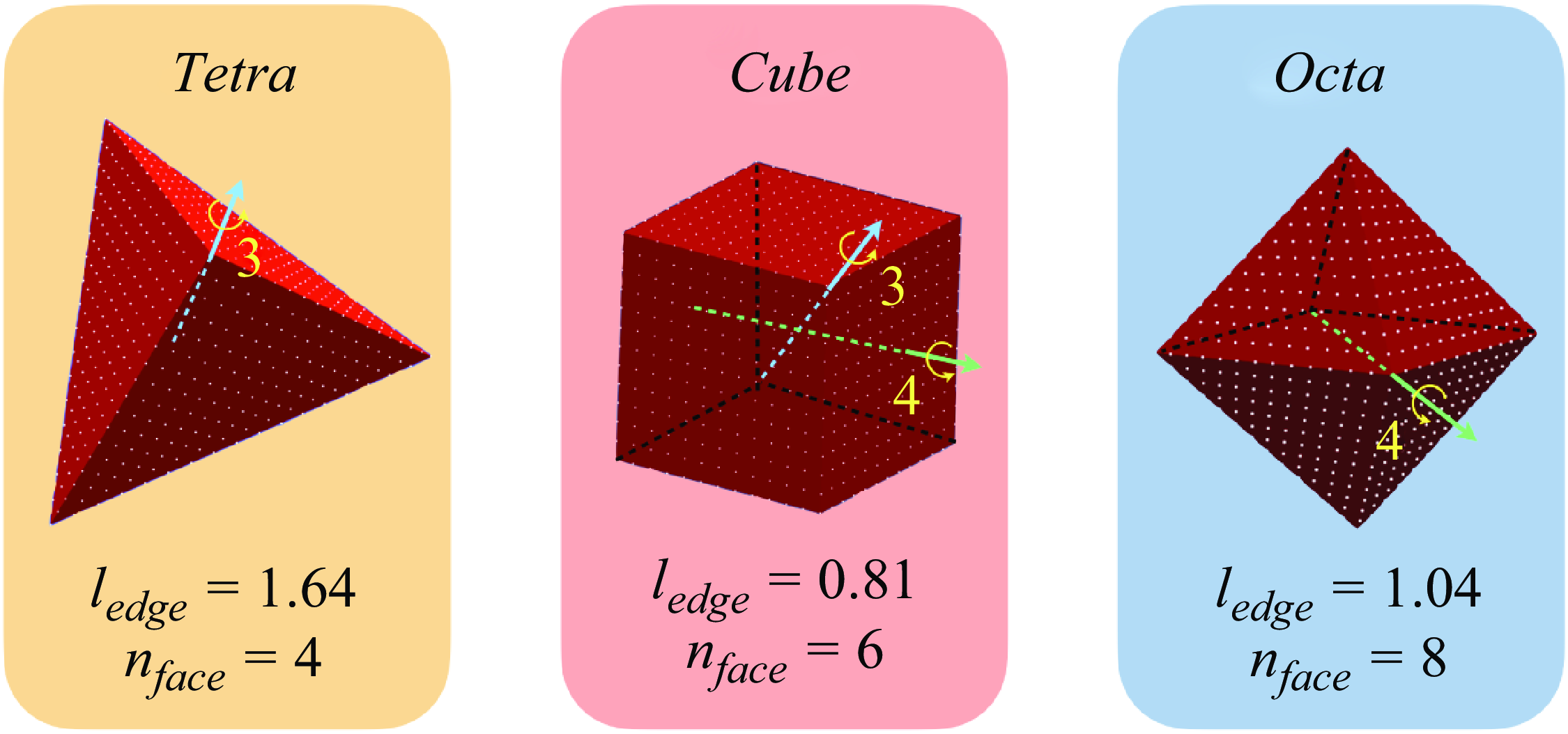
Figure 2. Distribution of Lagrange multipliers (white dots) on the surface of three Platonic polyhedrons (tetrahedron $\phi =0.67$
, cube
$\phi =0.67$
, cube $\phi =0.806$
and octahedron
$\phi =0.806$
and octahedron $\phi =0.846$
), illustrating their edge lengths (
$\phi =0.846$
), illustrating their edge lengths ( $l_{edge}$
), number of faces (
$l_{edge}$
), number of faces ( $n_{\textit{face}}$
) and axis of rotation with their corresponding number of rotational symmetry folds.
$n_{\textit{face}}$
) and axis of rotation with their corresponding number of rotational symmetry folds.
In this study, we use a collocation point method (Glowinski et al. Reference Glowinski, Pan, Hesla and Joseph1999; Wachs et al. Reference Wachs, Hammouti, Vinay and Rahmani2015; Gai & Wachs Reference Gai and Wachs2023a
) within the DLM/FD solver to enforce rigid-body motion constraints on three Platonic polyhedrons, as depicted in figure 2. The point set comprises interior points, which are grid nodes situated inside the particle, as well as surface points. It is shown that the surface of the tetrahedron and of the octahedron consists of triangular faces, while the surface of the cube consists of square faces. The surface points are uniformly distributed parallel to the edges on the particle surface. Despite being isometric, these three angular particles exhibit distinct interaction dynamics with the flow at different angular positions. To investigate the transverse rotation of these particles, we choose several rotation axes with different symmetry fold $n_{\Omega }$
: a three-fold rotational symmetry axis for the tetrahedron (referred to as RTF3), both three-fold and four-fold rotational symmetry axis for the cube (RCF3 and RCF4), and a four-fold rotational symmetry axis for the octahedron (ROF4), as shown in figure 2. For a better resolution of the sharp edges and corners, we strategically place points along all the edges and vertices of the particles. We use a consistent point-to-point distance of
$n_{\Omega }$
: a three-fold rotational symmetry axis for the tetrahedron (referred to as RTF3), both three-fold and four-fold rotational symmetry axis for the cube (RCF3 and RCF4), and a four-fold rotational symmetry axis for the octahedron (ROF4), as shown in figure 2. For a better resolution of the sharp edges and corners, we strategically place points along all the edges and vertices of the particles. We use a consistent point-to-point distance of $l_{pp} = 2\Delta x$
, aligning with the smallest grid cell size around the particle. As the refinement level
$l_{pp} = 2\Delta x$
, aligning with the smallest grid cell size around the particle. As the refinement level $n_l$
increases, more surface points are added on the particle. This distribution approach, known as the parallel point set, has been demonstrated to provide satisfactory spatial accuracy (Wachs et al. Reference Wachs, Hammouti, Vinay and Rahmani2015) and can be effectively applied to angular particles (Gai & Wachs Reference Gai and Wachs2023a
,Reference Gai and Wachs
b
).
$n_l$
increases, more surface points are added on the particle. This distribution approach, known as the parallel point set, has been demonstrated to provide satisfactory spatial accuracy (Wachs et al. Reference Wachs, Hammouti, Vinay and Rahmani2015) and can be effectively applied to angular particles (Gai & Wachs Reference Gai and Wachs2023a
,Reference Gai and Wachs
b
).
As already pointed out earlier in this section, we use the advective time scale $t_{ref}^* = D_{sph}^*/U_{ref}^*$
as the characteristic time scale. In terms of time resolution, the dimensionless time step
$t_{ref}^* = D_{sph}^*/U_{ref}^*$
as the characteristic time scale. In terms of time resolution, the dimensionless time step $\Delta t = \Delta t^*/t_{ref}^*$
is kept below
$\Delta t = \Delta t^*/t_{ref}^*$
is kept below $5 \times 10^{-3}$
in all our simulations to minimise numerical errors introduced by the operator splitting algorithm. For slowly rotating particles with
$5 \times 10^{-3}$
in all our simulations to minimise numerical errors introduced by the operator splitting algorithm. For slowly rotating particles with $\Omega \leqslant 0.1$
, the time step is set to
$\Omega \leqslant 0.1$
, the time step is set to $\Delta t = 5 \times 10^{-3}$
to ensure a sufficient number of complete rotation periods for accurate time-averaging at the post-processing level. When
$\Delta t = 5 \times 10^{-3}$
to ensure a sufficient number of complete rotation periods for accurate time-averaging at the post-processing level. When $\Omega \gt 0.1$
, a smaller time step of
$\Omega \gt 0.1$
, a smaller time step of $\Delta t = 5 \times 10^{-4}$
is used to provide enough frames per rotation period, thereby enhancing numerical accuracy and eliminating unphysical oscillations. Additionally, we ensure numerical stability by satisfying the Courant–Friedrichs–Lewy (CFL) condition, which is necessary for the explicit treatment of the advective term in the momentum conservation equation. The time step
$\Delta t = 5 \times 10^{-4}$
is used to provide enough frames per rotation period, thereby enhancing numerical accuracy and eliminating unphysical oscillations. Additionally, we ensure numerical stability by satisfying the Courant–Friedrichs–Lewy (CFL) condition, which is necessary for the explicit treatment of the advective term in the momentum conservation equation. The time step $\Delta t$
is dynamically updated according to the following formula:
$\Delta t$
is dynamically updated according to the following formula:
 \begin{equation} \Delta t = \left \{ \begin{array}{l} \displaystyle {\min \left ( \: 5\times 10^{-3}\:,\: \min _{i} \frac {0.8\Delta x_i^*}{\big | {\boldsymbol{u}}_i^* t_{ref}^*\big |} \: \right )\,\, \mbox{for}\,\,\Omega \leqslant 0.1}, \\ \\ \displaystyle {\min \left ( \: 5\times 10^{-4}\:,\: \min _{i} \frac {0.8\Delta x_i^*}{\big | {\boldsymbol{u}}_i^* t_{ref}^*\big |} \: \right )\,\, \mbox{for}\,\,\Omega \gt 0.1}. \end{array} \right . \end{equation}
In this formula, $i$
denotes a grid cell index and the minimum operator performs over all grid cells. By simulating over a sufficiently long physical time, we ensure that the flow regimes are fully developed. Additional information on the time convergence validation can be found in Appendix B.
$i$
denotes a grid cell index and the minimum operator performs over all grid cells. By simulating over a sufficiently long physical time, we ensure that the flow regimes are fully developed. Additional information on the time convergence validation can be found in Appendix B.
3. Flow past a rotating sphere
Prior to discussing the flow past a rotating angular particle, we analyse the behaviour of a rotating sphere in an inertial flow. Figure 3 shows the evolution of the time-averaged drag coefficient $\overline {C_d}$
and lift coefficient
$\overline {C_d}$
and lift coefficient $\overline {C_{l,y}}$
for a transversely rotating sphere in flows at
$\overline {C_{l,y}}$
for a transversely rotating sphere in flows at ${{R}e} = 100$
,
${{R}e} = 100$
, $300$
and
$300$
and $500$
, with our numerical results depicted by solid lines. Note that the temporal evolution of
$500$
, with our numerical results depicted by solid lines. Note that the temporal evolution of $C_d$
and
$C_d$
and $C_{l,y}$
can exhibit oscillatory behaviour due to vortex shedding in the wake. To obtain reliable estimates of
$C_{l,y}$
can exhibit oscillatory behaviour due to vortex shedding in the wake. To obtain reliable estimates of $\overline {C_d}$
and
$\overline {C_d}$
and $\overline {C_{l,y}}$
, we compute their time-averaged values over a sufficiently long period after the transient behaviour has subsided. For a given
$\overline {C_{l,y}}$
, we compute their time-averaged values over a sufficiently long period after the transient behaviour has subsided. For a given ${R}e$
, both
${R}e$
, both $\overline {C_d}$
and
$\overline {C_d}$
and $\overline {C_{l,y}}$
increase as the rotation rate
$\overline {C_{l,y}}$
increase as the rotation rate $\Omega$
varies from
$\Omega$
varies from $0.05$
to
$0.05$
to $1$
. In figure 3(a), it is shown that
$1$
. In figure 3(a), it is shown that $\overline {C_d}$
attains lower values as flow inertia increases from
$\overline {C_d}$
attains lower values as flow inertia increases from ${{R}e}=100$
to
${{R}e}=100$
to ${{R}e}=500$
. Figure 3(b) shows that
${{R}e}=500$
. Figure 3(b) shows that $\overline {C_{l,y}}$
exhibits a clear decreasing trend with
$\overline {C_{l,y}}$
exhibits a clear decreasing trend with ${R}e$
when
${R}e$
when $\Omega \gt 0.25$
. The data reported in the literature (Giacobello et al. Reference Giacobello, Ooi and Balachandar2009; Poon et al. Reference Poon, Ooi, Giacobello, Iaccarino and Chung2014) are presented with scatter points using the colour matching the solid lines for the corresponding
$\Omega \gt 0.25$
. The data reported in the literature (Giacobello et al. Reference Giacobello, Ooi and Balachandar2009; Poon et al. Reference Poon, Ooi, Giacobello, Iaccarino and Chung2014) are presented with scatter points using the colour matching the solid lines for the corresponding ${{R}e} = 100$
,
${{R}e} = 100$
, $300$
and
$300$
and $500$
. Overall, our numerical results are in excellent agreement with those reported in the literature.
$500$
. Overall, our numerical results are in excellent agreement with those reported in the literature.
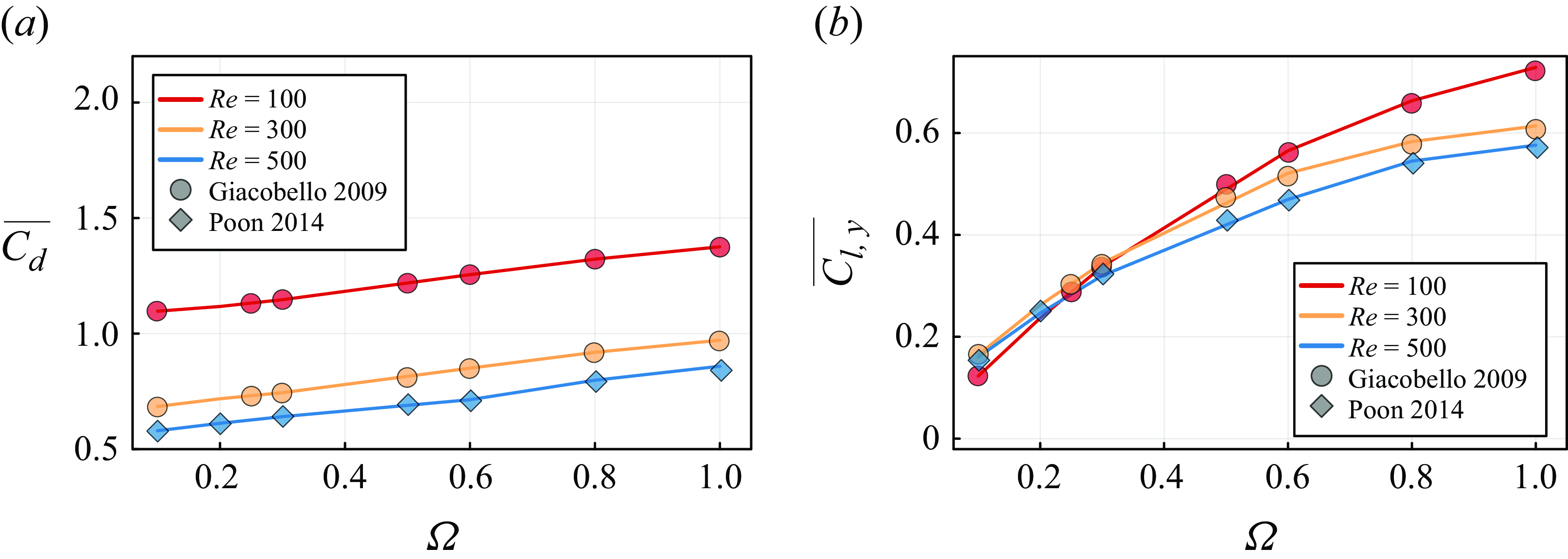
Figure 3. Validation of the evolution of $\overline {C_d}$
and
$\overline {C_d}$
and $\overline {C_{l,y}}$
as a function of
$\overline {C_{l,y}}$
as a function of $\Omega$
in the flow past a rotating sphere. The solid lines represent our numerical results at different Reynolds numbers
$\Omega$
in the flow past a rotating sphere. The solid lines represent our numerical results at different Reynolds numbers $100 \leqslant {{R}e} \leqslant 500$
. These results are compared with the data from Giacobello et al. (Reference Giacobello, Ooi and Balachandar2009) and Poon et al. (Reference Poon, Ooi, Giacobello, Iaccarino and Chung2014), shown by markers of matching colours.
$100 \leqslant {{R}e} \leqslant 500$
. These results are compared with the data from Giacobello et al. (Reference Giacobello, Ooi and Balachandar2009) and Poon et al. (Reference Poon, Ooi, Giacobello, Iaccarino and Chung2014), shown by markers of matching colours.
4. Flow past a rotating cube
4.1. Flow regime transition
We start by presenting an overview of the regimes for 143 simulations of flow past a transversely rotating cube (RCF4) performed in this study. The regime transition map depicted in figure 4 illustrates how the wake structure evolves across the range of rotation rate $0.02 \leqslant \Omega \leqslant 1$
and Reynolds numbers
$0.02 \leqslant \Omega \leqslant 1$
and Reynolds numbers $40 \leqslant {{R}e} \leqslant 400$
. Flow regimes are represented by colour-coded rectangles, with the upper and lower bounds of
$40 \leqslant {{R}e} \leqslant 400$
. Flow regimes are represented by colour-coded rectangles, with the upper and lower bounds of $\Omega$
clearly marked, offering a visual representation of the flow transitions. We distinguish and discuss the following flow regimes.
$\Omega$
clearly marked, offering a visual representation of the flow transitions. We distinguish and discuss the following flow regimes.
-
(i) Steady vortical regime (SV,
 ): the wake region of the particle displays a steady, typically straight vortical structure.
 -
(ii) Unsteady vortical regime (UV,
): the wake flow exhibits unsteady, fragmented vortical structures with irregular sizes. -
(iii) Periodic hairpin vortex shedding regime (HS,
): the particle wake structure manifests periodic hairpin vortex shedding, maintaining a planar symmetry with respect to the
$x$
-
$y$
plane passing through the particle centroid. -
(iv) Vortex suppression regime (VS,
): vortex shedding is suppressed due to the rotation of the particle, where the wake vortical structure becomes straight and steady. -
(v) Shear-induced vortex shedding regime (KH,
): fluctus vortical structures form in the far-field wake of the particle, arising from Kelvin–Helmholtz instability. -
(vi) Double shear-induced shedding regime (DS,
): the wake structure exhibits a second shear-induced vortex tail, in addition to the vortical structures caused by Kelvin–Helmholtz instability. -
(vii) Chaotic shedding regime (CS,
): the wake structure becomes unpredictable and irregular, losing its planar symmetry and exhibiting chaotic vortex shedding due to the increased fluid inertia.


Figure 4. Regime map of the flow past the transversely rotating RCF4 cube at $40 \leqslant {{R}e} \leqslant 400$
and
$40 \leqslant {{R}e} \leqslant 400$
and $0.02 \leqslant \Omega \leqslant 1$
: steady vortical (SV,
$0.02 \leqslant \Omega \leqslant 1$
: steady vortical (SV,
![]() ), unsteady vortical (UV,
), unsteady vortical (UV,
![]() ), periodic hairpin vortex shedding (HS,
), periodic hairpin vortex shedding (HS,
![]() ), vortex suppression (VS,
), vortex suppression (VS,
![]() ), shear-induced shedding (KH,
), shear-induced shedding (KH,
![]() ), double shear-induced shedding (DS,
), double shear-induced shedding (DS,
![]() ) and chaotic shedding (CS,
) and chaotic shedding (CS,
![]() ) regime.
) regime.
At very low rotation rate, $\Omega = 0.02$
, the flow past a rotating cube undergoes a sequence of regime transitions as
$\Omega = 0.02$
, the flow past a rotating cube undergoes a sequence of regime transitions as ${R}e$
increases: SV, UV, HS and ultimately CS at high
${R}e$
increases: SV, UV, HS and ultimately CS at high ${R}e$
. At low flow inertia
${R}e$
. At low flow inertia ${{R}e} = 40{-} 100$
, slow particle rotation
${{R}e} = 40{-} 100$
, slow particle rotation $\Omega \leqslant 0.2$
promotes the formation of vortical structures and their periodic shedding in the particle wake. As the rotation rate increases to
$\Omega \leqslant 0.2$
promotes the formation of vortical structures and their periodic shedding in the particle wake. As the rotation rate increases to $\Omega = 0.3$
, vortex shedding in the particle wake is suppressed, marking the onset of the VS regime. With increasing flow inertia, the suppressed wake structure becomes unsteady at high rotation rates due to the K-H instability, a phenomenon caused by velocity shear between the particle wake and the bulk flow. The KH regime emerges at
$\Omega = 0.3$
, vortex shedding in the particle wake is suppressed, marking the onset of the VS regime. With increasing flow inertia, the suppressed wake structure becomes unsteady at high rotation rates due to the K-H instability, a phenomenon caused by velocity shear between the particle wake and the bulk flow. The KH regime emerges at $\textit{Re} = 120$
and
$\textit{Re} = 120$
and $\Omega = 1$
. From
$\Omega = 1$
. From $\textit{Re} = 160$
to
$\textit{Re} = 160$
to $\textit{Re} = 200$
, both the HS and KH regimes expand, gradually replacing the VS regime in the range
$\textit{Re} = 200$
, both the HS and KH regimes expand, gradually replacing the VS regime in the range $0.3 \leqslant \Omega \leqslant 0.8$
. At
$0.3 \leqslant \Omega \leqslant 0.8$
. At ${{R}e} = 250$
and
${{R}e} = 250$
and $\Omega = 0.8$
, a second shear-induced vortex tail appears in the upper wake, marking the onset of the DS regime. Beyond
$\Omega = 0.8$
, a second shear-induced vortex tail appears in the upper wake, marking the onset of the DS regime. Beyond ${{R}e} = 250$
, the HS, KH and DS regimes are superseded by the CS regime due to the increased flow instability. At
${{R}e} = 250$
, the HS, KH and DS regimes are superseded by the CS regime due to the increased flow instability. At ${{R}e} = 400$
, the flow past a rotating cube still exhibits periodic, organised wake structures in the HS and KH regimes at
${{R}e} = 400$
, the flow past a rotating cube still exhibits periodic, organised wake structures in the HS and KH regimes at $\Omega = 0.2$
and
$\Omega = 0.2$
and $0.3$
, while all other cases transition to chaotic behaviour. Overall, we observe that a moderate rotation rate, particularly in the range of
$0.3$
, while all other cases transition to chaotic behaviour. Overall, we observe that a moderate rotation rate, particularly in the range of $\Omega = 0.2 \sim 0.4$
, either stabilises or reorganises the wake: at low
$\Omega = 0.2 \sim 0.4$
, either stabilises or reorganises the wake: at low ${R}e$
, it leads to vortex suppression, while at high
${R}e$
, it leads to vortex suppression, while at high ${R}e$
, it restructures the wake into periodic shedding within a highly unsteady flow.
${R}e$
, it restructures the wake into periodic shedding within a highly unsteady flow.
4.2. Vortex generation on the cube
4.2.1. Slowly rotating cube
To better understand the regime transitions and wake stability in the flow past a transversely rotating cube, it is important to first clarify the mechanism of vortex generation on the cube. In the RCF4 configuration, the transversely rotating cube has two primary angular positions: one with a face directly facing the incoming flow and the other with an edge (dividing two front faces) facing the flow. We consider an extreme case where the cube is fixed in the flow at these two angular positions and illustrate the corresponding streamwise vorticity $\omega _x$
generation in figure 5(a). Here, the choice of
$\omega _x$
generation in figure 5(a). Here, the choice of $\omega _x$
is motivated by its higher sensitivity to wake structure evolution, enabling more accurate and precise characterisation of the wake dynamics (Gai & Wachs Reference Gai and Wachs2023a
).
$\omega _x$
is motivated by its higher sensitivity to wake structure evolution, enabling more accurate and precise characterisation of the wake dynamics (Gai & Wachs Reference Gai and Wachs2023a
).

Figure 5. Vortex generation mechanism on the surface and in the wake of the slowly rotating RCF4 cube. (a) Schematic of vortex generation on the front surface (left subpanels with black backgrounds) and in the wake of fixed cubes (right subpanels with white backgrounds), with one edge and one face facing the incoming flow ( $x^+$
direction). In all subpanels, red and blue regions indicate positive and negative
$x^+$
direction). In all subpanels, red and blue regions indicate positive and negative $\omega _x$
, respectively. (b) Regime transition sequence for a slowly rotating cube at
$\omega _x$
, respectively. (b) Regime transition sequence for a slowly rotating cube at ${{R}e}=60$
and
${{R}e}=60$
and $\Omega = 0.02$
, compared with the regime transition in the flow past a fixed cube with an edge or a face facing the flow. The temporal evolution of the vorticity pattern
$\Omega = 0.02$
, compared with the regime transition in the flow past a fixed cube with an edge or a face facing the flow. The temporal evolution of the vorticity pattern $\omega _x$
in the particle wake is illustrated, along with side views of the isosurfaces
$\omega _x$
in the particle wake is illustrated, along with side views of the isosurfaces $\omega _x = \pm 0.03$
.
$\omega _x = \pm 0.03$
.
As thoroughly discussed in our previous work (Gai & Wachs Reference Gai and Wachs2023d
), an inclined front face of the fixed angular particle generates a pair of counter-rotating streamwise vortices $\omega _x$
. For example, when the cube has an edge facing the flow, one pair of vortices (
$\omega _x$
. For example, when the cube has an edge facing the flow, one pair of vortices ( $\omega _1$
,
$\omega _1$
, $\omega _2$
) forms on the upper front face, while a second pair (
$\omega _2$
) forms on the upper front face, while a second pair ( $\omega _3$
,
$\omega _3$
, $\omega _4$
) forms on the lower front face. These two vortex pairs are then advected into the wake of the cube, maintaining a typical pattern of two vortex pairs (shown in blue and red) as depicted in figure 5(a). When a square face of the cube is oriented perpendicular to the flow, four pairs of oppositely signed streamwise vortices are generated. In addition to the two pairs formed on the upper and lower faces of the cube, two more vortex pairs appear on the side faces: the pair (
$\omega _4$
) forms on the lower front face. These two vortex pairs are then advected into the wake of the cube, maintaining a typical pattern of two vortex pairs (shown in blue and red) as depicted in figure 5(a). When a square face of the cube is oriented perpendicular to the flow, four pairs of oppositely signed streamwise vortices are generated. In addition to the two pairs formed on the upper and lower faces of the cube, two more vortex pairs appear on the side faces: the pair ( $\omega _5$
,
$\omega _5$
, $\omega _6$
) on the left side face and the pair (
$\omega _6$
) on the left side face and the pair ( $\omega _7$
,
$\omega _7$
, $\omega _8$
) on the right face. Although these side vortex pairs are also generated in the edge facing the flow configuration, their intensity is significantly lower and much less visible compared with the vortices produced on the upper and lower faces.
$\omega _8$
) on the right face. Although these side vortex pairs are also generated in the edge facing the flow configuration, their intensity is significantly lower and much less visible compared with the vortices produced on the upper and lower faces.
Now, we rotate the cube slowly at $\Omega =0.02$
around the
$\Omega =0.02$
around the $z$
-axis to observe how the vorticity pattern in the particle wake evolves with time. In figure 5(b), we present several snapshots of the temporal evolution of the
$z$
-axis to observe how the vorticity pattern in the particle wake evolves with time. In figure 5(b), we present several snapshots of the temporal evolution of the $\omega _x$
pattern in the
$\omega _x$
pattern in the $y$
-
$y$
- $z$
plane at
$z$
plane at $x=x_p + 1.5$
(
$x=x_p + 1.5$
( $x_p$
denotes the
$x_p$
denotes the $x$
coordinate of the particle centroid) for the case at
$x$
coordinate of the particle centroid) for the case at ${{R}e}=60$
in the upper panel. The side views of the isosurface
${{R}e}=60$
in the upper panel. The side views of the isosurface $\omega _x=\pm 0.03$
are illustrated in the bottom of the upper panel for better clarity. In the SV regime, the
$\omega _x=\pm 0.03$
are illustrated in the bottom of the upper panel for better clarity. In the SV regime, the $\omega _x$
patterns are planar and symmetric, exhibiting a high similarity to those in the fixed edge cube case shown in figure 5(a). The two pairs of streamwise vortices are clearly visible in the side view. We know that in the case of a fixed edge cube in the multi-axis steady symmetry regime (MSS,
$\omega _x$
patterns are planar and symmetric, exhibiting a high similarity to those in the fixed edge cube case shown in figure 5(a). The two pairs of streamwise vortices are clearly visible in the side view. We know that in the case of a fixed edge cube in the multi-axis steady symmetry regime (MSS,
![]() ), the four vortex filaments in the wake are of equal length and remain steady. With transverse rotation, the length of the vortex pairs evolves in time. The length of the vortex pair (
), the four vortex filaments in the wake are of equal length and remain steady. With transverse rotation, the length of the vortex pairs evolves in time. The length of the vortex pair ( $\omega _1$
,
$\omega _1$
, $\omega _2$
) is clearly shorter than that of the vortex pair (
$\omega _2$
) is clearly shorter than that of the vortex pair ( $\omega _3$
,
$\omega _3$
, $\omega _4$
) in the first snapshot I. In snapshot II, the upper vortex pair (
$\omega _4$
) in the first snapshot I. In snapshot II, the upper vortex pair ( $\omega _1$
,
$\omega _1$
, $\omega _2$
) becomes longer instead. In the following, we will demonstrate how the reciprocal motion of vortex pairs and the evolution of their relative strength can explain the vortex suppression.
$\omega _2$
) becomes longer instead. In the following, we will demonstrate how the reciprocal motion of vortex pairs and the evolution of their relative strength can explain the vortex suppression.
The similarity between the slowly rotating cube and a fixed edge cube can also be observed from the regime map. In the lower panel of figure 5(b), we present the regime map of flow past an edge and a face cube for ${{R}e}=40{-} 400$
. In place of the SV and UV regimes, the fixed cube exhibits the MSS (
${{R}e}=40{-} 400$
. In place of the SV and UV regimes, the fixed cube exhibits the MSS (
![]() ) and the planar steady symmetry regime (PSS,
) and the planar steady symmetry regime (PSS,
![]() ), respectively. It is evident that the regime transition sequence of the slowly rotating cube shows very similar critical
), respectively. It is evident that the regime transition sequence of the slowly rotating cube shows very similar critical ${R}e$
for the first two regime transitions as those observed for the fixed edge cube, rather than those observed for the fixed face cube. At higher
${R}e$
for the first two regime transitions as those observed for the fixed edge cube, rather than those observed for the fixed face cube. At higher ${R}e$
, rotation causes flow instability to occur earlier (at
${R}e$
, rotation causes flow instability to occur earlier (at ${{R}e}=300$
) compared with the fixed edge cube (at
${{R}e}=300$
) compared with the fixed edge cube (at ${{R}e}=340$
).
${{R}e}=340$
).
4.2.2. Vortex merging induced by rotation
Unlike the multi-axis symmetry typically observed in the wake of a fixed cube, the particle rotation promotes the merging of surface vortices, resulting in a planar symmetry of vortex distribution, even at low Reynolds numbers such as ${{R}e}=60$
. The merging process occurs once the vortices are generated on the front surface of the cube. In figure 6, we present the
${{R}e}=60$
. The merging process occurs once the vortices are generated on the front surface of the cube. In figure 6, we present the $\omega _x$
distribution in the
$\omega _x$
distribution in the $y$
-
$y$
- $z$
plane at
$z$
plane at $x = x_p - 0.1$
for flows at
$x = x_p - 0.1$
for flows at ${{R}e}=60$
,
${{R}e}=60$
, $160$
,
$160$
, $350$
and
$350$
and $\Omega =0.02{-} 1$
. We highlight the vortex cores by setting the colour bar to
$\Omega =0.02{-} 1$
. We highlight the vortex cores by setting the colour bar to $\omega _x \in [-1,1]$
, where regions with higher magnitude of
$\omega _x \in [-1,1]$
, where regions with higher magnitude of $\omega _x$
are represented by red and blue, while areas with values close to
$\omega _x$
are represented by red and blue, while areas with values close to $0$
appear in black.
$0$
appear in black.

Figure 6. Visualisation of vortex merging on the front surface of the rotating RCF4 cube in the $y$
-
$y$
- $z$
plane at
$z$
plane at $x = x_p - 0.1$
, with red and blue regions representing positive and negative
$x = x_p - 0.1$
, with red and blue regions representing positive and negative $\omega _x$
, respectively. Flow streamlines are included to enhance the visualisation of the wake vortices. The various flow regimes are highlighted in colour-coded boxes, and the cube projected outline on the
$\omega _x$
, respectively. Flow streamlines are included to enhance the visualisation of the wake vortices. The various flow regimes are highlighted in colour-coded boxes, and the cube projected outline on the $y$
-
$y$
- $z$
plane is sketched for reference.
$z$
plane is sketched for reference.
In the case of ${{R}e}=60$
and
${{R}e}=60$
and $\Omega =0.02$
, we observe the generation of four pairs of streamwise vortices (
$\Omega =0.02$
, we observe the generation of four pairs of streamwise vortices ( $\omega _1 - \omega _8$
) similar to the fixed cube case in figure 5(a). Under the cube rotation in figure 6, the two side vortices
$\omega _1 - \omega _8$
) similar to the fixed cube case in figure 5(a). Under the cube rotation in figure 6, the two side vortices $\omega _5$
and
$\omega _5$
and $\omega _8$
are fairly weak and get pushed away from the cube surface by their opposite-signed counter-parts
$\omega _8$
are fairly weak and get pushed away from the cube surface by their opposite-signed counter-parts $\omega _6$
and
$\omega _6$
and $\omega _7$
, respectively. This gives room for the vortex
$\omega _7$
, respectively. This gives room for the vortex $\omega _6$
to spread on the left side of the cube and to reach its arm to its neighbour of the same positive sign, the stronger
$\omega _6$
to spread on the left side of the cube and to reach its arm to its neighbour of the same positive sign, the stronger $\omega _4$
generated by the lower face. We observe the same mechanism between
$\omega _4$
generated by the lower face. We observe the same mechanism between $\omega _7$
and
$\omega _7$
and $\omega _3$
. This process depicts the initiation of the surface vortex merging
$\omega _3$
. This process depicts the initiation of the surface vortex merging $\omega _4 \cup \omega _6$
and
$\omega _4 \cup \omega _6$
and $\omega _3 \cup \omega _7$
that play key roles in the wake stability of the rotating cube. With the increase of the rotation rate, at
$\omega _3 \cup \omega _7$
that play key roles in the wake stability of the rotating cube. With the increase of the rotation rate, at ${{R}e}=60$
and
${{R}e}=60$
and $\Omega =0.1$
, we observe that the weak side vortices
$\Omega =0.1$
, we observe that the weak side vortices $\omega _5$
and
$\omega _5$
and $\omega _8$
, which are pushed away from the side faces, find their way to reach their neighbours of the same sign,
$\omega _8$
, which are pushed away from the side faces, find their way to reach their neighbours of the same sign, $\omega _1$
and
$\omega _1$
and $\omega _2$
from the upper face, respectively. A second merging process takes place on the top of the cube, but slightly away from the surface, resulting in the vortex structure
$\omega _2$
from the upper face, respectively. A second merging process takes place on the top of the cube, but slightly away from the surface, resulting in the vortex structure $\omega _1 \cup \omega _5$
and
$\omega _1 \cup \omega _5$
and $\omega _2 \cup \omega _8$
as depicted at
$\omega _2 \cup \omega _8$
as depicted at ${{R}e}=60$
and
${{R}e}=60$
and $\Omega = 0.3$
. We note that all the investigated cases exhibit these two types of rotation-induced vortex merging processes on the cube front surface, resulting in an inner pair and an outer pair of streamwise vortices propagating to the wake.
$\Omega = 0.3$
. We note that all the investigated cases exhibit these two types of rotation-induced vortex merging processes on the cube front surface, resulting in an inner pair and an outer pair of streamwise vortices propagating to the wake.
It is worth mentioning that some variations of the merging process may occur. At low rotating rate, such as $\Omega =0.02$
, we observe that the merging of the outer vortex may not happen, this is visible in the cases
$\Omega =0.02$
, we observe that the merging of the outer vortex may not happen, this is visible in the cases ${{R}e}=160$
and
${{R}e}=160$
and ${{R}e}=350$
in figure 6. In the HS regime, the periodic vortex shedding takes place, and we note that the roles of the inner and outer vortex pairs can swap in time. For instance, in the snapshot of the case at
${{R}e}=350$
in figure 6. In the HS regime, the periodic vortex shedding takes place, and we note that the roles of the inner and outer vortex pairs can swap in time. For instance, in the snapshot of the case at ${{R}e}=160$
and
${{R}e}=160$
and $\Omega =0.1$
, the merged vortex
$\Omega =0.1$
, the merged vortex $\omega _1 \cup \omega _5$
appears on the cube surface while vortex
$\omega _1 \cup \omega _5$
appears on the cube surface while vortex $\omega _6$
is pushed away to meet
$\omega _6$
is pushed away to meet $\omega _4$
, due to the larger inclination angle of the upper face. As the cube continues to rotate, we see that the merged vortex
$\omega _4$
, due to the larger inclination angle of the upper face. As the cube continues to rotate, we see that the merged vortex $\omega _1 \cup \omega _5$
moves aways from the side face, while the merged vortex
$\omega _1 \cup \omega _5$
moves aways from the side face, while the merged vortex $\omega _4 \cup \omega _6$
returns to the surface, similar to the snapshot at
$\omega _4 \cup \omega _6$
returns to the surface, similar to the snapshot at ${{R}e}=60$
and
${{R}e}=60$
and $\Omega =0.1$
. With the increase of the rotation rate,
$\Omega =0.1$
. With the increase of the rotation rate, $\Omega \geqslant 0.4$
, the impact of the cube angular position diminishes, and the alternating role swap ceases. The merged vortices
$\Omega \geqslant 0.4$
, the impact of the cube angular position diminishes, and the alternating role swap ceases. The merged vortices $\omega _4 \cup \omega _6$
and
$\omega _4 \cup \omega _6$
and $\omega _3 \cup \omega _7$
consistently form the inner pair, as observed in the KH regime at
$\omega _3 \cup \omega _7$
consistently form the inner pair, as observed in the KH regime at ${{R}e} = 160$
,
${{R}e} = 160$
, $\Omega = 0.8$
and
$\Omega = 0.8$
and $\Omega = 1$
. In the CS regime, even though the planar symmetry is broken on the front surface, the merging process still follows the same mechanism, as shown in the case
$\Omega = 1$
. In the CS regime, even though the planar symmetry is broken on the front surface, the merging process still follows the same mechanism, as shown in the case ${{R}e}=350$
and
${{R}e}=350$
and $\Omega =0.8$
in figure 6.
$\Omega =0.8$
in figure 6.
4.2.3. Near-wake vortex structures
Now that we clarified the vortex generation and merging process, we present in figure 7 the $\omega _x$
distribution in the particle wake region in the
$\omega _x$
distribution in the particle wake region in the $y$
-
$y$
- $z$
plane, right next to the rear face at
$z$
plane, right next to the rear face at $x = x_p + 0.6$
. At this point, the interaction between the vortices and the particle surface terminates. The evolution of the wake structure is driven solely by fluid dynamics and vortex interactions. Four Reynolds numbers (
$x = x_p + 0.6$
. At this point, the interaction between the vortices and the particle surface terminates. The evolution of the wake structure is driven solely by fluid dynamics and vortex interactions. Four Reynolds numbers ( ${{R}e} = 60 {-} 350$
) are selected to illustrate the wake vortices across the seven flow regimes studied. The same colour scale (
${{R}e} = 60 {-} 350$
) are selected to illustrate the wake vortices across the seven flow regimes studied. The same colour scale ( $\omega _x \in [-1,1]$
) as that used in figure 6 is used for consistency and better comparison. Regions in red and blue indicate higher vorticity magnitude, while black areas represent lower vorticity magnitude. In the case
$\omega _x \in [-1,1]$
) as that used in figure 6 is used for consistency and better comparison. Regions in red and blue indicate higher vorticity magnitude, while black areas represent lower vorticity magnitude. In the case ${{R}e} = 60$
and
${{R}e} = 60$
and $\Omega = 0.02$
, the vortex pattern appears blurred due to the low vortex strength.
$\Omega = 0.02$
, the vortex pattern appears blurred due to the low vortex strength.

Figure 7. Visualisation of vortex pair generation near the rear surface of the rotating RCF4 cube in the $y$
-
$y$
- $z$
plane at
$z$
plane at $x = x_p + 0.6$
, with red and blue regions representing positive and negative
$x = x_p + 0.6$
, with red and blue regions representing positive and negative $\omega _x$
, respectively. Flow streamlines are included to enhance the visualisation of the wake vortices. The various flow regimes are highlighted in colour-coded boxes, and the projected outline of the cube on the
$\omega _x$
, respectively. Flow streamlines are included to enhance the visualisation of the wake vortices. The various flow regimes are highlighted in colour-coded boxes, and the projected outline of the cube on the $y$
-
$y$
- $z$
plane is sketched for reference.
$z$
plane is sketched for reference.
At low flow inertia, ${{R}e} = 60$
, the merged vortex pairs near the cube surface,
${{R}e} = 60$
, the merged vortex pairs near the cube surface, $\omega _{46}$
(hereafter denoting the merged vortex
$\omega _{46}$
(hereafter denoting the merged vortex $\omega _4 \cup \omega _6$
) and
$\omega _4 \cup \omega _6$
) and $\omega _{37}$
(hereafter denoting the merged vortex
$\omega _{37}$
(hereafter denoting the merged vortex $\omega _3 \cup \omega _7$
), exhibit dominant magnitudes and maintain symmetry with respect to the
$\omega _3 \cup \omega _7$
), exhibit dominant magnitudes and maintain symmetry with respect to the $x$
-
$x$
- $y$
plane across the cube centroid. A higher
$y$
plane across the cube centroid. A higher $\Omega$
enhances
$\Omega$
enhances $\omega _x$
, particularly in the VS regime, highlighted by the pink box in the first row of figure 7. In this regime, periodic vortex shedding is suppressed by the cube rotation, resulting in a steady vorticity distribution that only includes the vortex pairs
$\omega _x$
, particularly in the VS regime, highlighted by the pink box in the first row of figure 7. In this regime, periodic vortex shedding is suppressed by the cube rotation, resulting in a steady vorticity distribution that only includes the vortex pairs $\omega _{46}$
and
$\omega _{46}$
and $\omega _{37}$
, as seen in the case
$\omega _{37}$
, as seen in the case ${{R}e} = 60$
and
${{R}e} = 60$
and $\Omega = 0.6$
. At
$\Omega = 0.6$
. At ${{R}e} = 160$
and
${{R}e} = 160$
and ${{R}e} = 250$
, particularly in the UV and HS regimes, we observe the formation of the outer vortex pairs
${{R}e} = 250$
, particularly in the UV and HS regimes, we observe the formation of the outer vortex pairs $\omega _{15}$
and
$\omega _{15}$
and $\omega _{28}$
, originating from the upper front surface of the cube, as shown in the cases at
$\omega _{28}$
, originating from the upper front surface of the cube, as shown in the cases at $\Omega = 0.3$
. In the HS regime, the periodic interactions between the inner and outer vortex pairs result in a variety of vorticity distribution patterns, as illustrated in figure 7.
$\Omega = 0.3$
. In the HS regime, the periodic interactions between the inner and outer vortex pairs result in a variety of vorticity distribution patterns, as illustrated in figure 7.
At ${{R}e} = 160$
, increasing the rotation rate to
${{R}e} = 160$
, increasing the rotation rate to $\Omega = 0.4$
results in relatively weak outer vortex pairs
$\Omega = 0.4$
results in relatively weak outer vortex pairs $\omega _{15}$
and
$\omega _{15}$
and $\omega _{28}$
, as they are pushed away from the wake, marking the onset of the VS regime. In the KH regime indicated by the blue box, at
$\omega _{28}$
, as they are pushed away from the wake, marking the onset of the VS regime. In the KH regime indicated by the blue box, at $\Omega = 0.8$
and
$\Omega = 0.8$
and $\Omega = 1$
, the magnitude of
$\Omega = 1$
, the magnitude of $\omega _{15}$
and
$\omega _{15}$
and $\omega _{28}$
increases again, and they tightly wrap around the inner vortex pair like tulip petals. A similar vorticity pattern is also observed in the DS regime at
$\omega _{28}$
increases again, and they tightly wrap around the inner vortex pair like tulip petals. A similar vorticity pattern is also observed in the DS regime at ${{R}e} = 250$
and
${{R}e} = 250$
and ${{R}e} = 350$
, as shown in the green box in figure 7. In the DS regime, a second shear-induced vortical tail forms in the wake, with the vortex cores of this second tail clearly visible at
${{R}e} = 350$
, as shown in the green box in figure 7. In the DS regime, a second shear-induced vortical tail forms in the wake, with the vortex cores of this second tail clearly visible at $\Omega = 1$
for both
$\Omega = 1$
for both ${{R}e} = 250$
and
${{R}e} = 250$
and ${{R}e} = 350$
. Overall, the near-wake vortex structure maintains a planar or pseudo-planar symmetry with respect to the
${{R}e} = 350$
. Overall, the near-wake vortex structure maintains a planar or pseudo-planar symmetry with respect to the $x$
-
$x$
- $y$
plane, except in cases within the CS regime.
$y$
plane, except in cases within the CS regime.
In summary, the generation and merging of vortex pairs on the particle surface dictate the near-wake vortex patterns, which in turn influence the formation, dynamics and stability of the wake vortical structures, thereby shaping the flow regimes. Our findings demonstrate that the formation of two vortex pairs – inner and outer – is a universal process across all flow regimes within the investigated parameter space.
4.3. Wake vortical structures
Once formed at the particle surface, the streamwise vortices are advected into the wake region, where they develop into complex vortical structures. In the following sections, we will closely examine the interactions between these wake structures, with a focus on gaining new insights into how the sharp edges of the cube influence wake flow instability.
4.3.1. Vortex shedding and suppression
We recall that behind a transversely rotating sphere, the particle rotation amplifies wake unsteadiness, leading to periodic hairpin vortex shedding at lower critical ${R}e$
compared with a fixed sphere. This shedding follows a characteristic build-up and release process. As
${R}e$
compared with a fixed sphere. This shedding follows a characteristic build-up and release process. As $\Omega$
increases, the vortices in the recirculation region disappear, and vortex shedding is suppressed within
$\Omega$
increases, the vortices in the recirculation region disappear, and vortex shedding is suppressed within $0.3 \leqslant \Omega \leqslant 0.5$
for
$0.3 \leqslant \Omega \leqslant 0.5$
for ${{R}e} = 100 {-} 300$
(Giacobello et al. Reference Giacobello, Ooi and Balachandar2009). Beyond this suppression, at higher values of both
${{R}e} = 100 {-} 300$
(Giacobello et al. Reference Giacobello, Ooi and Balachandar2009). Beyond this suppression, at higher values of both $\Omega$
and
$\Omega$
and ${R}e$
, the steady vortical tail becomes unsteady once again, driven by a Kelvin–Helmholtz instability.
${R}e$
, the steady vortical tail becomes unsteady once again, driven by a Kelvin–Helmholtz instability.
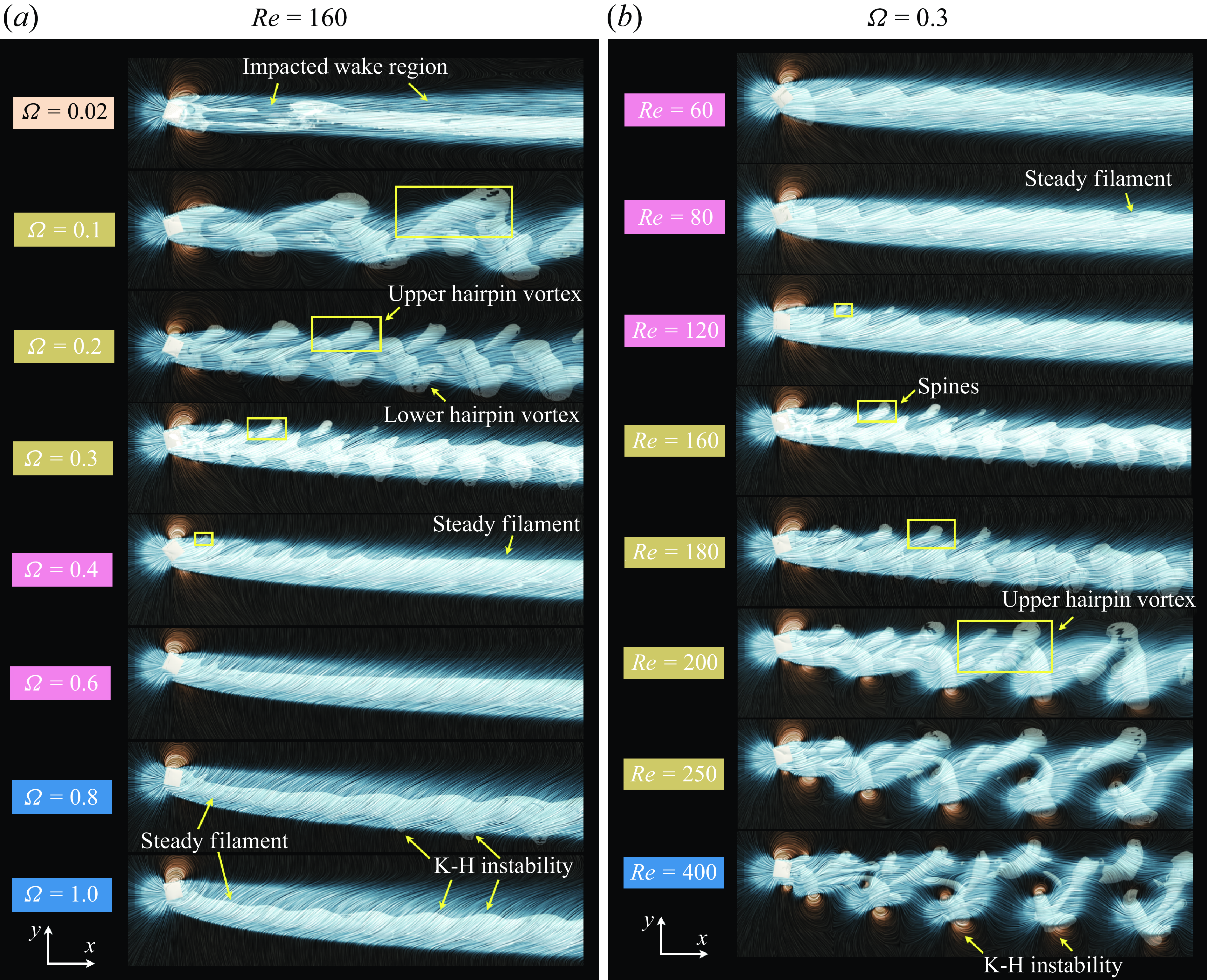
Figure 8. Vortical structures identified by $\lambda _2=-1$
in the wake of the rotating RCF4 cube (a) at
$\lambda _2=-1$
in the wake of the rotating RCF4 cube (a) at ${{R}e}=160$
and (b) at
${{R}e}=160$
and (b) at $\Omega =0.3$
in the
$\Omega =0.3$
in the $x$
-
$x$
- $y$
plane. The red and blue regions indicate positive and negative disturbed velocity,
$y$
plane. The red and blue regions indicate positive and negative disturbed velocity, $\tilde {u}_x \in [-0.1,0.1]$
, respectively. Flow streamlines based on
$\tilde {u}_x \in [-0.1,0.1]$
, respectively. Flow streamlines based on $\boldsymbol{\tilde {u}}$
are plotted to enhance the clarity of the wake flow field. The different flow regimes are distinguished by colour-coded boxes on the left of each subpanel.
$\boldsymbol{\tilde {u}}$
are plotted to enhance the clarity of the wake flow field. The different flow regimes are distinguished by colour-coded boxes on the left of each subpanel.
How different are the wake structures of a rotating angular particle compared with those of a rotating sphere? To investigate this, we present snapshots of the vortical structures behind a rotating cube in the $x$
-
$x$
- $y$
plane, as shown in figure 8. The vortex structures are identified using the isosurface
$y$
plane, as shown in figure 8. The vortex structures are identified using the isosurface $\lambda _2 = -1$
. Due to the dominance of the streamwise incoming velocity over the other velocity components, important details of the wake region may be obscured. To better capture the wake dynamics, we plot the streamlines of the disturbed flow velocity
$\lambda _2 = -1$
. Due to the dominance of the streamwise incoming velocity over the other velocity components, important details of the wake region may be obscured. To better capture the wake dynamics, we plot the streamlines of the disturbed flow velocity $\boldsymbol{\tilde {u}} = (\boldsymbol{u^*} - U^*_{ref}\boldsymbol{e_x}) / U^*_{ref}$
and colour these streamlines using the scale of
$\boldsymbol{\tilde {u}} = (\boldsymbol{u^*} - U^*_{ref}\boldsymbol{e_x}) / U^*_{ref}$
and colour these streamlines using the scale of $\tilde {u}_x \in [-0.1, 0.1]$
, to reveal more details of the wake region.
$\tilde {u}_x \in [-0.1, 0.1]$
, to reveal more details of the wake region.
As an example, figure 8(a) illustrates the evolution of wake structures with increasing rotation rates $0.02 \leqslant \Omega \leqslant 1$
at
$0.02 \leqslant \Omega \leqslant 1$
at ${{R}e} = 160$
. The flow regime transitions from UV to HS, VS and eventually KH, following a sequence similar to that observed for a sphere. At
${{R}e} = 160$
. The flow regime transitions from UV to HS, VS and eventually KH, following a sequence similar to that observed for a sphere. At $\Omega = 0.02$
, the wake behind the rotating cube appears straight, with fragmented vortical structures shed from the cube at a low frequency. Beneath the vortical structures, a broad, elongated strip region (
$\Omega = 0.02$
, the wake behind the rotating cube appears straight, with fragmented vortical structures shed from the cube at a low frequency. Beneath the vortical structures, a broad, elongated strip region ( $\tilde {u}_x \leqslant 0$
) is visible in light blue, extending behind the cube. This impacted wake region, present in all subpanels of figure 8, encloses the wake vortical structures and defines the boundary of the disturbed wake flow. As the rotation rate increases to
$\tilde {u}_x \leqslant 0$
) is visible in light blue, extending behind the cube. This impacted wake region, present in all subpanels of figure 8, encloses the wake vortical structures and defines the boundary of the disturbed wake flow. As the rotation rate increases to $\Omega = 0.1 {-}0.3$
, hairpin vortex shedding occurs with increasing frequency.
$\Omega = 0.1 {-}0.3$
, hairpin vortex shedding occurs with increasing frequency.
A notable difference from the rotating sphere case is that the vortex shedding frequency behind a rotating cube is significantly higher at the same ${R}e$
and
${R}e$
and $\Omega$
. Two distinct types of vortex structures are observed: upper hairpin vortices originate from the upper front face of the rotating cube, while lower hairpin vortices emerge from the lower front face and side faces. Compared with
$\Omega$
. Two distinct types of vortex structures are observed: upper hairpin vortices originate from the upper front face of the rotating cube, while lower hairpin vortices emerge from the lower front face and side faces. Compared with $\Omega = 0.2$
, the wake vortex structures become smaller at
$\Omega = 0.2$
, the wake vortex structures become smaller at $\Omega = 0.3$
. In the highlighted yellow rectangles, it is clear that the size of the upper hairpin vortices decreases with increasing
$\Omega = 0.3$
. In the highlighted yellow rectangles, it is clear that the size of the upper hairpin vortices decreases with increasing $\Omega$
, disappearing entirely at
$\Omega$
, disappearing entirely at $\Omega = 0.4$
, where wake vortex shedding is suppressed and manifests as a steady filament. Some residual bumpy structures remain near the top rear face of the cube at
$\Omega = 0.4$
, where wake vortex shedding is suppressed and manifests as a steady filament. Some residual bumpy structures remain near the top rear face of the cube at $\Omega = 0.4$
, but they vanish completely at
$\Omega = 0.4$
, but they vanish completely at $\Omega = 0.6$
. At higher rotation rates, the fluctus structures resulting from the Kelvin–Helmholtz instability are observed along the steady filaments near the lower boundary of the impacted wake region at
$\Omega = 0.6$
. At higher rotation rates, the fluctus structures resulting from the Kelvin–Helmholtz instability are observed along the steady filaments near the lower boundary of the impacted wake region at $\Omega = 0.8$
and
$\Omega = 0.8$
and $\Omega = 1$
.
$\Omega = 1$
.
In terms of flow inertia, we present the evolution of wake vortical structures in the $x$
-
$x$
- $y$
plane at the same
$y$
plane at the same $\Omega = 0.3$
while varying the Reynolds number in the range
$\Omega = 0.3$
while varying the Reynolds number in the range $60 \leqslant {{R}e} \leqslant 400$
in figure 8(b). We focus on the influence of flow inertia on wake instability, particularly in cases where vortex shedding is suppressed in the VS regime. At
$60 \leqslant {{R}e} \leqslant 400$
in figure 8(b). We focus on the influence of flow inertia on wake instability, particularly in cases where vortex shedding is suppressed in the VS regime. At ${{R}e} = 60$
and
${{R}e} = 60$
and ${{R}e} = 80$
, the
${{R}e} = 80$
, the $\lambda _2$
isosurface shows bumpy structures near the rear surface of the cube, but it stabilises into a steady filament in the far-wake region of the cube; this is not the case at
$\lambda _2$
isosurface shows bumpy structures near the rear surface of the cube, but it stabilises into a steady filament in the far-wake region of the cube; this is not the case at $\Omega = 0.2$
and the same
$\Omega = 0.2$
and the same ${R}e$
. Thus, we classify these cases in the VS regime, where vortex suppression is effective. As
${R}e$
. Thus, we classify these cases in the VS regime, where vortex suppression is effective. As ${R}e$
increases, vortex shedding reemerges, and the size of the vortical structures grows with
${R}e$
increases, vortex shedding reemerges, and the size of the vortical structures grows with ${R}e$
. At
${R}e$
. At ${{R}e} = 120$
, small spine-like structures appear along the top boundary of the impacted wake region near the cube rear surface, highlighted in yellow rectangles in figure 8(b). As
${{R}e} = 120$
, small spine-like structures appear along the top boundary of the impacted wake region near the cube rear surface, highlighted in yellow rectangles in figure 8(b). As ${R}e$
increases, the spine structures grow in size and gradually evolve into upper hairpin vortices, as depicted in the HS regime at
${R}e$
increases, the spine structures grow in size and gradually evolve into upper hairpin vortices, as depicted in the HS regime at ${{R}e} = 200$
. This process reverses the vortex suppression highlighted in the yellow rectangles in figure 8(a). Specifically, the spines (or upper hairpin vortices) generated by the upper front face of the rotating cube are suppressed as
${{R}e} = 200$
. This process reverses the vortex suppression highlighted in the yellow rectangles in figure 8(a). Specifically, the spines (or upper hairpin vortices) generated by the upper front face of the rotating cube are suppressed as $\Omega$
increases, but as flow inertia rises, these vortices reemerge through a reversed yet similar mechanism. Between
$\Omega$
increases, but as flow inertia rises, these vortices reemerge through a reversed yet similar mechanism. Between ${{R}e} = 180$
and
${{R}e} = 180$
and ${{R}e} = 200$
, the vortex shedding frequency noticeably decreases and remains constant up to
${{R}e} = 200$
, the vortex shedding frequency noticeably decreases and remains constant up to ${{R}e} = 400$
. At this point, the hairpin vortical structures become more complex, while still maintaining periodicity and symmetry about the
${{R}e} = 400$
. At this point, the hairpin vortical structures become more complex, while still maintaining periodicity and symmetry about the $x$
-
$x$
- $y$
plane.
$y$
plane.
From figure 8, it is clear that the sharp edges of the rotating cube, particularly those on the upper front face, play a critical role in both the suppression and reemergence of vortex shedding. These edges strongly influence the generation of vortices, which in turn drive flow instabilities through their interactions in the wake region. To better understand these interactions, we examine the evolution of streamwise vortex pairs $\omega _x$
in the
$\omega _x$
in the $x$
-
$x$
- $z$
plane, visualised by isosurfaces at
$z$
plane, visualised by isosurfaces at $\omega _x = \pm 0.03$
(with red indicating positive
$\omega _x = \pm 0.03$
(with red indicating positive $\omega _x$
and blue indicating negative
$\omega _x$
and blue indicating negative $\omega _x$
) for
$\omega _x$
) for $40 \leqslant {{R}e} \leqslant 200$
and
$40 \leqslant {{R}e} \leqslant 200$
and $0.1 \leqslant \Omega \leqslant 0.8$
in figure 9. Our analysis focuses on the case at
$0.1 \leqslant \Omega \leqslant 0.8$
in figure 9. Our analysis focuses on the case at $\Omega = 0.3$
and
$\Omega = 0.3$
and ${{R}e} = 120$
, while reducing the transparency of other cases for enhanced clarity.
${{R}e} = 120$
, while reducing the transparency of other cases for enhanced clarity.
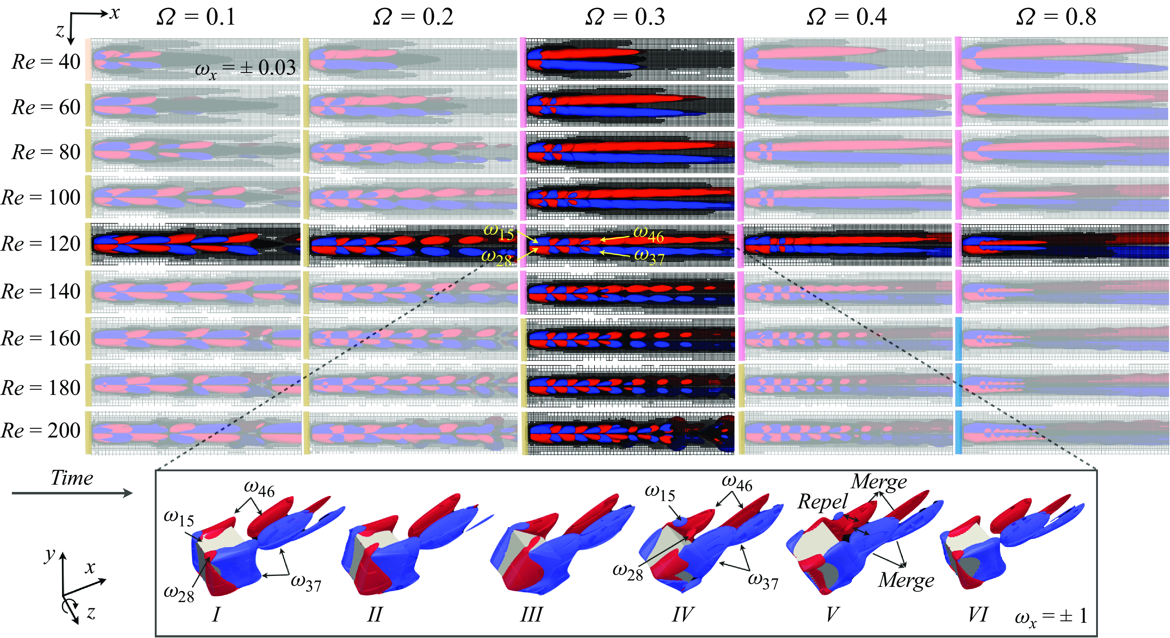
Figure 9. Evolution of streamwise vortex pairs identified by isosurfaces of $\omega _x=\pm 0.03$
(red for positive
$\omega _x=\pm 0.03$
(red for positive $\omega _x$
and blue for negative
$\omega _x$
and blue for negative $\omega _x$
) in the
$\omega _x$
) in the $x$
-
$x$
- $z$
plane. Lower panel shows snapshots of temporal evolution of the core of the vortex pairs identified by
$z$
plane. Lower panel shows snapshots of temporal evolution of the core of the vortex pairs identified by $\omega _x=\pm 1$
within a single rotation period.
$\omega _x=\pm 1$
within a single rotation period.
The flow past a rotating cube generates alternating vortex pairs of opposite sign in the $x$
-
$x$
- $z$
plane. As discussed in figure 7, one vortex pair, consisting of
$z$
plane. As discussed in figure 7, one vortex pair, consisting of $\omega _{15}$
and
$\omega _{15}$
and $\omega _{28}$
, originates from the upper front face of the cube and is located in the upper region of the wake (relative to the
$\omega _{28}$
, originates from the upper front face of the cube and is located in the upper region of the wake (relative to the $y$
-axis). The other pair,
$y$
-axis). The other pair, $\omega _{46}$
and
$\omega _{46}$
and $\omega _{37}$
, forms from the merging of vortices generated by the lower front and side faces, and resides in the lower region of the wake. These two vortex pairs are shed alternately into the wake, as highlighted in yellow at
$\omega _{37}$
, forms from the merging of vortices generated by the lower front and side faces, and resides in the lower region of the wake. These two vortex pairs are shed alternately into the wake, as highlighted in yellow at ${{R}e} = 120$
and
${{R}e} = 120$
and $\Omega = 0.3$
in figure 9.
$\Omega = 0.3$
in figure 9.
Considering ${{R}e} = 120$
, at a low rotation rate
${{R}e} = 120$
, at a low rotation rate $\Omega = 0.1$
, the size of the upper vortex pair (
$\Omega = 0.1$
, the size of the upper vortex pair ( $\omega _{15}$
,
$\omega _{15}$
, $\omega _{28}$
) is comparable to that of the lower vortex pair (
$\omega _{28}$
) is comparable to that of the lower vortex pair ( $\omega _{46}$
,
$\omega _{46}$
, $\omega _{37}$
), leading to a standard periodic hairpin vortex shedding. As
$\omega _{37}$
), leading to a standard periodic hairpin vortex shedding. As $\Omega$
increases, with the rotation vector aligned along the
$\Omega$
increases, with the rotation vector aligned along the $z$
-axis, the first direct effect is a reduction in fluid–particle relative velocity on the upper side (
$z$
-axis, the first direct effect is a reduction in fluid–particle relative velocity on the upper side ( $y^+$
) of the cube, while the relative velocity on the lower side (
$y^+$
) of the cube, while the relative velocity on the lower side ( $y^-$
) increases (within the range
$y^-$
) increases (within the range $\Omega \leqslant 1$
in this study). This weakens the upper vortex pair (
$\Omega \leqslant 1$
in this study). This weakens the upper vortex pair ( $\omega _{15}$
,
$\omega _{15}$
, $\omega _{28}$
) while strengthening the lower vortex pair (
$\omega _{28}$
) while strengthening the lower vortex pair ( $\omega _{46}$
,
$\omega _{46}$
, $\omega _{37}$
). Another key point is that, during each rotation period, four faces of the cube contribute to the generation of the upper vortex pair, with each face producing one. These faces are referred to as effective faces, and their number, denoted as
$\omega _{37}$
). Another key point is that, during each rotation period, four faces of the cube contribute to the generation of the upper vortex pair, with each face producing one. These faces are referred to as effective faces, and their number, denoted as $N_{\mathcal{F}}$
, depends on the particle shape and the axis of rotation. The effective faces directly determine the primary shedding frequency of the vortex pairs, which is typically proportional to
$N_{\mathcal{F}}$
, depends on the particle shape and the axis of rotation. The effective faces directly determine the primary shedding frequency of the vortex pairs, which is typically proportional to $N_{\mathcal{F}}$
, a distinctive feature of rotating angular particles. Hence, with
$N_{\mathcal{F}}$
, a distinctive feature of rotating angular particles. Hence, with $\Omega$
increasing from
$\Omega$
increasing from $0.1$
to
$0.1$
to $0.2$
in the HS regime, the shedding frequency doubles. As a result of these combined effects, at
$0.2$
in the HS regime, the shedding frequency doubles. As a result of these combined effects, at $\Omega =0.3$
, the lower vortex pair shedding becomes more frequent and stronger, resulting in vortex merging in the wake. In the upper wake, the upper vortex pair is too weak to pinch off its lower counterpart. This imbalance results in a long, steady vortical tail with two filaments in the VS regime, explaining the vortex suppression, which persists up to
$\Omega =0.3$
, the lower vortex pair shedding becomes more frequent and stronger, resulting in vortex merging in the wake. In the upper wake, the upper vortex pair is too weak to pinch off its lower counterpart. This imbalance results in a long, steady vortical tail with two filaments in the VS regime, explaining the vortex suppression, which persists up to $\Omega =1$
at
$\Omega =1$
at ${{R}e}=120$
.
${{R}e}=120$
.
In the lower panel of figure 9, we present six snapshots of the vortex pair shedding process over a single rotation period for the flow at ${{R}e}=120$
and
${{R}e}=120$
and $\Omega =0.3$
, shown from a side view. The positions of the upper and lower vortex pairs are indicated. To improve the clarity of the visualisation, the vorticity isosurface criterion has been increased to
$\Omega =0.3$
, shown from a side view. The positions of the upper and lower vortex pairs are indicated. To improve the clarity of the visualisation, the vorticity isosurface criterion has been increased to $\omega _x = \pm 1$
to better highlight the vortex cores. At
$\omega _x = \pm 1$
to better highlight the vortex cores. At $\Omega = 0.3$
, the upper vortex pair (
$\Omega = 0.3$
, the upper vortex pair ( $\omega _{15}$
,
$\omega _{15}$
, $\omega _{28}$
) is clearly weaker than the lower vortex pair (
$\omega _{28}$
) is clearly weaker than the lower vortex pair ( $\omega _{46}$
,
$\omega _{46}$
, $\omega _{37}$
), as seen in snapshot I. As the cube keeps rotating, snapshots IV and V show the interaction between the upper and lower vortex pairs. Due to their opposite signs,
$\omega _{37}$
), as seen in snapshot I. As the cube keeps rotating, snapshots IV and V show the interaction between the upper and lower vortex pairs. Due to their opposite signs, $\omega _{15}$
and
$\omega _{15}$
and $\omega _{46}$
repel each other in space, as do
$\omega _{46}$
repel each other in space, as do $\omega _{28}$
and
$\omega _{28}$
and $\omega _{37}$
. In snapshots V and VI, the upper vortex pair is pushed away and dissipates due to diffusion, while the two successive lower vortex pairs begin to merge. The presence of the weak upper vortex pair acts as wedges on the strong lower pair isosurface and leads to the formation of the spine structures observed in figure 8. As
$\omega _{37}$
. In snapshots V and VI, the upper vortex pair is pushed away and dissipates due to diffusion, while the two successive lower vortex pairs begin to merge. The presence of the weak upper vortex pair acts as wedges on the strong lower pair isosurface and leads to the formation of the spine structures observed in figure 8. As ${R}e$
increases, the upper vortex pairs strengthen and grow in size, significantly influencing the wake stability. At
${R}e$
increases, the upper vortex pairs strengthen and grow in size, significantly influencing the wake stability. At ${{R}e} = 160$
, their increased presence becomes substantial enough to prevent the merging of the lower vortex pairs, thereby leading to the HS regime. Consequently, the reemergence of periodic vortex shedding follows the same mechanism as previously discussed, but in reverse.
${{R}e} = 160$
, their increased presence becomes substantial enough to prevent the merging of the lower vortex pairs, thereby leading to the HS regime. Consequently, the reemergence of periodic vortex shedding follows the same mechanism as previously discussed, but in reverse.
In summary, our results provide a clear explanation for vortex suppression and reemergence mechanism through the lens of vortex interaction. The alternating shedding of upper and lower vortex pairs characterises the periodic hairpin vortex formation, while the merging of the lower vortex pair is the primary mechanism behind vortex suppression. The weakened upper vortex pairs are responsible for the formation of spine structures in the wake. Compared with the smooth geometry of a sphere, the sharp edges and distinct faces of the rotating cube provide a clearer understanding of the roles played by the upper and lower vortex pairs in these processes.
4.3.2. Wake structures in high-
${R}e$
regimes


Figure 10. Vortical structures identified by $\lambda _2=-1$
in the wake of the rotating RCF4 cube at (a)
$\lambda _2=-1$
in the wake of the rotating RCF4 cube at (a) ${{R}e}=250$
, (b)
${{R}e}=250$
, (b) ${{R}e}=300$
and (c)
${{R}e}=300$
and (c) ${{R}e}=400$
. The red and blue regions indicate positive and negative disturbed velocity,
${{R}e}=400$
. The red and blue regions indicate positive and negative disturbed velocity, $\tilde {u}_x \in [-0.1,0.1]$
, respectively. Flow streamlines based on
$\tilde {u}_x \in [-0.1,0.1]$
, respectively. Flow streamlines based on $\boldsymbol{\tilde {u}}$
are plotted to enhance the clarity of the wake vortex patterns. The different flow regimes are distinguished by colour-coded boxes, corresponding to each rotation rate.
$\boldsymbol{\tilde {u}}$
are plotted to enhance the clarity of the wake vortex patterns. The different flow regimes are distinguished by colour-coded boxes, corresponding to each rotation rate.
A remarkable feature of the flow past an angular particle is the wide variety of vortex shedding patterns that form in the wake. At high flow inertia, specifically when ${{R}e} \geqslant 250$
, the rotation of the cube introduces new dynamics in the wake structures, leading to distinct flow regimes. In figure 10, we present snapshots of these complex vortical structures and shedding patterns for
${{R}e} \geqslant 250$
, the rotation of the cube introduces new dynamics in the wake structures, leading to distinct flow regimes. In figure 10, we present snapshots of these complex vortical structures and shedding patterns for ${{R}e} \geqslant 250$
in the
${{R}e} \geqslant 250$
in the $x$
-
$x$
- $y$
plane. The streamlines of the disturbed velocity field
$y$
plane. The streamlines of the disturbed velocity field $\boldsymbol{\tilde {u}}$
are drawn to provide a clearer depiction.
$\boldsymbol{\tilde {u}}$
are drawn to provide a clearer depiction.
At ${{R}e}=250$
, as shown in figure 10(a), vortices follow a classical periodic hairpin vortex shedding pattern in the HS regime for
${{R}e}=250$
, as shown in figure 10(a), vortices follow a classical periodic hairpin vortex shedding pattern in the HS regime for $0.02 \leqslant \Omega \leqslant 0.3$
. While the shedding frequency generally increases with
$0.02 \leqslant \Omega \leqslant 0.3$
. While the shedding frequency generally increases with $\Omega$
, a slight decrease is observed between
$\Omega$
, a slight decrease is observed between $\Omega =0.2$
and
$\Omega =0.2$
and $\Omega =0.3$
. Interestingly, at
$\Omega =0.3$
. Interestingly, at $\Omega =0.2$
, the upper and lower vortex pairs, which are similar in size, are shed in phase, leading to a double-symmetric hairpin vortex shedding (DHS regime), resembling the pattern observed in the flow past an edge tetrahedron (Gai & Wachs Reference Gai and Wachs2023b
). At
$\Omega =0.2$
, the upper and lower vortex pairs, which are similar in size, are shed in phase, leading to a double-symmetric hairpin vortex shedding (DHS regime), resembling the pattern observed in the flow past an edge tetrahedron (Gai & Wachs Reference Gai and Wachs2023b
). At $\Omega \leqslant 0.3$
, the impacted wake region (
$\Omega \leqslant 0.3$
, the impacted wake region ( $\tilde {u}_x\leqslant 0$
) no longer appears as a wide strip, instead displaying blue regions tightly surrounding the vortical structures. As
$\tilde {u}_x\leqslant 0$
) no longer appears as a wide strip, instead displaying blue regions tightly surrounding the vortical structures. As $\Omega$
increases, the flow transitions to the KH regime, and the impacted wake region once again takes on a long strip shape. In this regime, the upper vortex pairs are moderated by mechanisms discussed earlier but are not fully suppressed. The lower vortex pairs, due to high fluid inertia, are unable to merge. At
$\Omega$
increases, the flow transitions to the KH regime, and the impacted wake region once again takes on a long strip shape. In this regime, the upper vortex pairs are moderated by mechanisms discussed earlier but are not fully suppressed. The lower vortex pairs, due to high fluid inertia, are unable to merge. At $\Omega =0.4$
and
$\Omega =0.4$
and $\Omega =0.6$
, we observe the formation of fluctus at the lower boundary of the impacted wake region, where red zones indicate the part of streamwise acceleration of the vortex cores. It is evident that the shedding frequency of the shear-induced vortices is higher than that of the vortices released from the recirculation region at
$\Omega =0.6$
, we observe the formation of fluctus at the lower boundary of the impacted wake region, where red zones indicate the part of streamwise acceleration of the vortex cores. It is evident that the shedding frequency of the shear-induced vortices is higher than that of the vortices released from the recirculation region at $\Omega =0.3$
. As
$\Omega =0.3$
. As $\Omega$
increases further, the shear-induced vortex shedding stabilises at
$\Omega$
increases further, the shear-induced vortex shedding stabilises at $\Omega =0.8$
and
$\Omega =0.8$
and $\Omega =1$
. Interestingly, under high rotation rates, the upper vortex pairs become enhanced and tend to merge, forming a steady, elongated structure – referred to as the second tail – at
$\Omega =1$
. Interestingly, under high rotation rates, the upper vortex pairs become enhanced and tend to merge, forming a steady, elongated structure – referred to as the second tail – at ${{R}e}=250$
and
${{R}e}=250$
and $\Omega =1$
. Note that this secondary tail is located at the upper boundary of the impacted wake region, which also contains two filaments symmetric to the
$\Omega =1$
. Note that this secondary tail is located at the upper boundary of the impacted wake region, which also contains two filaments symmetric to the $x$
-
$x$
- $y$
plane. The emergence of the secondary tail marks the onset of the DS regime. Due to the interplay of the flow inertia and angular particle rotation, we obtain a steady flow at relatively high
$y$
plane. The emergence of the secondary tail marks the onset of the DS regime. Due to the interplay of the flow inertia and angular particle rotation, we obtain a steady flow at relatively high ${R}e$
and
${R}e$
and $\Omega$
.
$\Omega$
.
Figure 10(b) presents the vortex shedding pattern at ${{R}e}=300$
, where the CS regime kicks in. Even when the cube slowly rotates at
${{R}e}=300$
, where the CS regime kicks in. Even when the cube slowly rotates at $\Omega =0.02$
, the wake vortex distribution behind the cube is no longer planar symmetric. As
$\Omega =0.02$
, the wake vortex distribution behind the cube is no longer planar symmetric. As $\Omega$
increases, the wake structure reorganises and the HS regime is observed for
$\Omega$
increases, the wake structure reorganises and the HS regime is observed for $0.1 \leqslant \Omega \leqslant 0.3$
. Especially, the double-hairpin shedding is also observed for
$0.1 \leqslant \Omega \leqslant 0.3$
. Especially, the double-hairpin shedding is also observed for ${{R}e}=300$
and
${{R}e}=300$
and $\Omega =0.2$
. With further increase of
$\Omega =0.2$
. With further increase of $\Omega$
, we note that the shear-induced shedding becomes predominant at
$\Omega$
, we note that the shear-induced shedding becomes predominant at $\Omega =0.4$
and
$\Omega =0.4$
and $\Omega =0.6$
. The upper vortex pairs are much enhanced by the flow inertia compared with the case
$\Omega =0.6$
. The upper vortex pairs are much enhanced by the flow inertia compared with the case ${{R}e}=250$
in figure 10(a). At
${{R}e}=250$
in figure 10(a). At $\Omega =0.8$
, the interaction between the upper and lower vortices becomes irregular, eliminating planar symmetry. Interestingly, at
$\Omega =0.8$
, the interaction between the upper and lower vortices becomes irregular, eliminating planar symmetry. Interestingly, at $\Omega =1$
, the planar symmetry is restored and the DS regime emerges. However, both tails at the upper and lower boundaries of the impacted wake region become unsteady. At
$\Omega =1$
, the planar symmetry is restored and the DS regime emerges. However, both tails at the upper and lower boundaries of the impacted wake region become unsteady. At ${{R}e}=400$
, as shown in figure 10(c), the wake structure loses its periodicity in the CS regime, except at
${{R}e}=400$
, as shown in figure 10(c), the wake structure loses its periodicity in the CS regime, except at $\Omega =0.2$
and
$\Omega =0.2$
and $0.3$
. Compared with the wake patterns observed at
$0.3$
. Compared with the wake patterns observed at ${{R}e}=250$
and
${{R}e}=250$
and $300$
, the impacted wake region at
$300$
, the impacted wake region at $\Omega =1$
is less inclined and more aligned with the cube. Although a second tail is still present, the vortex shedding pattern becomes fully chaotic and irregular.
$\Omega =1$
is less inclined and more aligned with the cube. Although a second tail is still present, the vortex shedding pattern becomes fully chaotic and irregular.
To offer readers a more in-depth understanding of vortex shedding, suppression and wake instability, the wake structures in the flow past a rotating cube in the $x$
-
$x$
- $y$
plane are presented for additional selected cases in Appendix C.
$y$
plane are presented for additional selected cases in Appendix C.
4.4. Hydrodynamic forces on the cube
The previous analysis offers new insights into the dynamics of vortical structures in the wake of a rotating cube. As these vortices form and shed, they induce changes to the velocity and pressure fields, and these changes significantly impact the lift and drag forces. We now turn our attention to the hydrodynamic forces exerted by the surrounding fluid on the particle.
4.4.1. Magnus effect and lift coefficient
We know that the flow interaction with the cube is predominantly influenced by two factors: the flow inertia ${R}e$
and the rotation rate
${R}e$
and the rotation rate $\Omega$
. To quantitatively assess the impact of these factors, we plot the evolution of the time-averaged lift coefficient,
$\Omega$
. To quantitatively assess the impact of these factors, we plot the evolution of the time-averaged lift coefficient, $\overline {C_{l,y}}$
, as a function of
$\overline {C_{l,y}}$
, as a function of $\Omega$
for
$\Omega$
for $40 \leqslant {{R}e} \leqslant 200$
, as shown in figure 11(a). For higher flow inertia (
$40 \leqslant {{R}e} \leqslant 200$
, as shown in figure 11(a). For higher flow inertia ( ${{R}e} \geqslant 250$
), the evolution of
${{R}e} \geqslant 250$
), the evolution of $\overline {C_{l,y}}$
is presented separately in figure 11(b), using the same colour bar for clarity. To ensure accurate temporal averaging,
$\overline {C_{l,y}}$
is presented separately in figure 11(b), using the same colour bar for clarity. To ensure accurate temporal averaging, $\overline {C_{l,y}}$
is computed over a sufficiently long period once the flow has fully developed.
$\overline {C_{l,y}}$
is computed over a sufficiently long period once the flow has fully developed.
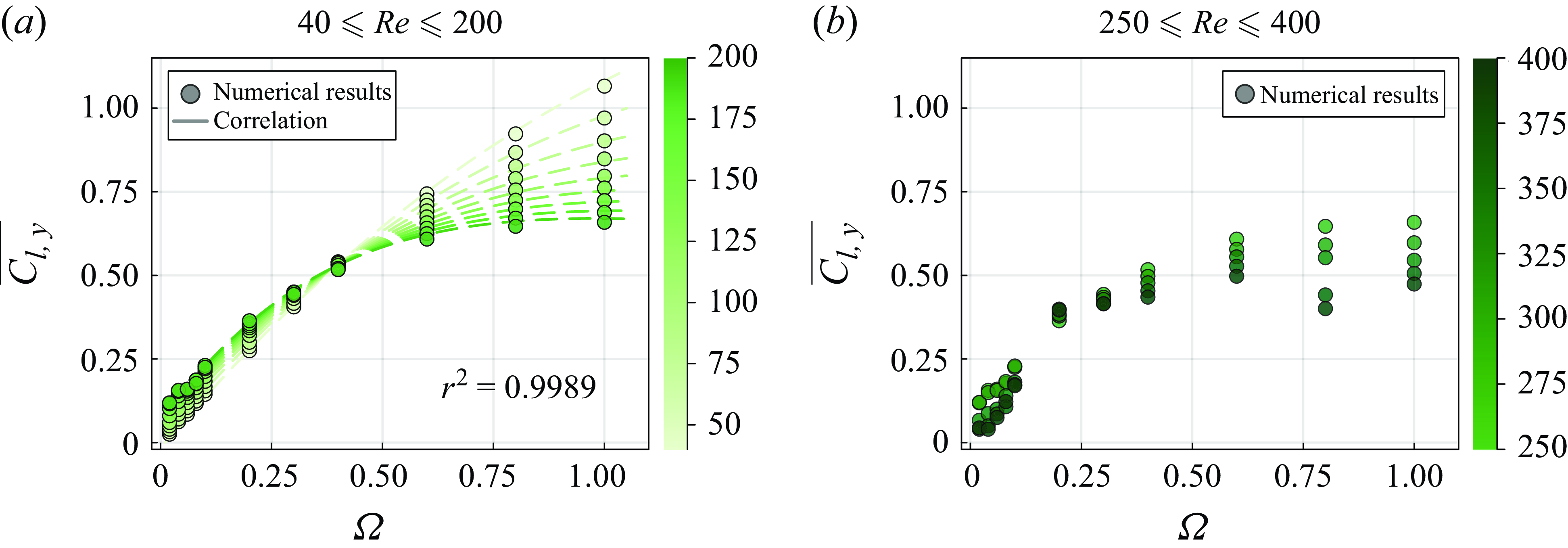
Figure 11. (a) Evolution of the time-averaged lift coefficient $\overline {C_{l,y}}$
of the rotating RCF4 cube as a function of
$\overline {C_{l,y}}$
of the rotating RCF4 cube as a function of $\Omega$
at
$\Omega$
at $40 \leqslant {{R}e} \leqslant 200$
with increment
$40 \leqslant {{R}e} \leqslant 200$
with increment $\Delta {{R}e}=20$
. Our numerical simulation results (coloured circles) are compared with the empirical correlation proposed in (4.1) (dashed lines). (b) Evolution of
$\Delta {{R}e}=20$
. Our numerical simulation results (coloured circles) are compared with the empirical correlation proposed in (4.1) (dashed lines). (b) Evolution of $\overline {C_{l,y}}$
at higher Reynolds numbers,
$\overline {C_{l,y}}$
at higher Reynolds numbers, $250 \leqslant {{R}e} \leqslant 400$
with increment
$250 \leqslant {{R}e} \leqslant 400$
with increment $\Delta {{R}e}=50$
. Darker circles indicate higher values of
$\Delta {{R}e}=50$
. Darker circles indicate higher values of ${R}e$
.
${R}e$
.
In general, increasing $\Omega$
results in a higher lift force due to the enhanced Magnus effect. The rotation of the cube causes a direct deceleration of the flow velocity on the bottom side (
$\Omega$
results in a higher lift force due to the enhanced Magnus effect. The rotation of the cube causes a direct deceleration of the flow velocity on the bottom side ( $y^-$
) compared with the top side (
$y^-$
) compared with the top side ( $y^+$
). According to Bernoulli’s principle, the higher velocity on the top corresponds to lower pressure, while the lower velocity on the bottom creates higher pressure, generating lift pointing to the
$y^+$
). According to Bernoulli’s principle, the higher velocity on the top corresponds to lower pressure, while the lower velocity on the bottom creates higher pressure, generating lift pointing to the $y^+$
direction. At low flow inertia, such as
$y^+$
direction. At low flow inertia, such as ${{R}e}=40$
,
${{R}e}=40$
, $\overline {C_{l,y}}$
increases almost linearly with
$\overline {C_{l,y}}$
increases almost linearly with $\Omega$
. With the increase of inertia, however, the increase in
$\Omega$
. With the increase of inertia, however, the increase in $\overline {C_{l,y}}$
becomes constrained, causing the curves to bend downward in figure 11(a). The influence of
$\overline {C_{l,y}}$
becomes constrained, causing the curves to bend downward in figure 11(a). The influence of ${R}e$
on
${R}e$
on $\overline {C_{l,y}}$
can be divided into two parts: for
$\overline {C_{l,y}}$
can be divided into two parts: for $\Omega \leqslant 0.4$
, the effect of
$\Omega \leqslant 0.4$
, the effect of ${R}e$
is small and tends to enhance
${R}e$
is small and tends to enhance $\overline {C_{l,y}}$
; for
$\overline {C_{l,y}}$
; for $\Omega \gt 0.4$
, higher
$\Omega \gt 0.4$
, higher ${R}e$
leads to a lower
${R}e$
leads to a lower $\overline {C_{l,y}}$
. A possible explanation is that the enhanced flow unsteadiness results in reducing the pressure difference between the top and bottom surfaces of the rotating cube, thereby diminishing the Magnus effect. Between
$\overline {C_{l,y}}$
. A possible explanation is that the enhanced flow unsteadiness results in reducing the pressure difference between the top and bottom surfaces of the rotating cube, thereby diminishing the Magnus effect. Between $\Omega =0.3$
and
$\Omega =0.3$
and $\Omega =0.4$
, we find a critical regime transition region where all the data points exhibit a very close value of
$\Omega =0.4$
, we find a critical regime transition region where all the data points exhibit a very close value of $\overline {C_{l,y}}$
. In this region, the rotation-driven time scale becomes smaller than the vortex formation time scale. We observe the complete suppression of vortex shedding and a reorganisation of the wake. The wake flow fully transitions from the HS regime to the VS regime (KH regime for
$\overline {C_{l,y}}$
. In this region, the rotation-driven time scale becomes smaller than the vortex formation time scale. We observe the complete suppression of vortex shedding and a reorganisation of the wake. The wake flow fully transitions from the HS regime to the VS regime (KH regime for ${{R}e}=180$
and
${{R}e}=180$
and ${{R}e}=200$
), as shown in figure 4. An extraordinary property of
${{R}e}=200$
), as shown in figure 4. An extraordinary property of $\Omega =0.4$
is that the lift coefficient
$\Omega =0.4$
is that the lift coefficient $\overline {C_{l,y}}$
becomes independent of
$\overline {C_{l,y}}$
becomes independent of ${R}e$
.
${R}e$
.
By incorporating ${R}e$
and
${R}e$
and $\Omega$
, we have developed an empirical correlation to predict
$\Omega$
, we have developed an empirical correlation to predict $\overline {C_{l,y}}$
through multivariable regression analysis:
$\overline {C_{l,y}}$
through multivariable regression analysis:
 \begin{equation} \overline {C_{l,y}} = 0.53 + {{R}e}^{-0.11}(2.02\Omega - 0.8)\exp (-0.017\Omega ^{1.08}{{R}e}^{0.86}). \end{equation}
Figure 11(a) shows that this correlation effectively captures the numerical results of $\overline {C_{l,y}}$
across the considered range of
$\overline {C_{l,y}}$
across the considered range of $40 \leqslant {{R}e} \leqslant 200$
and
$40 \leqslant {{R}e} \leqslant 200$
and $0.02 \leqslant \Omega \leqslant 1$
. The high determination coefficient,
$0.02 \leqslant \Omega \leqslant 1$
. The high determination coefficient, $R^2 = 0.9989$
, underscores the accuracy of the prediction. Furthermore, the model predicts that
$R^2 = 0.9989$
, underscores the accuracy of the prediction. Furthermore, the model predicts that $\overline {C_{l,y}}$
becomes independent of
$\overline {C_{l,y}}$
becomes independent of ${R}e$
at
${R}e$
at $\Omega \approxeq 0.4$
, where all curves converge to
$\Omega \approxeq 0.4$
, where all curves converge to $\overline {C_{l,y}}\approxeq 0.53$
, indicating a common point of overlap.
$\overline {C_{l,y}}\approxeq 0.53$
, indicating a common point of overlap.
At higher flow inertia, the lift coefficient exhibits a different behaviour with increasing ${R}e$
, potentially due to a bifurcation in the base flow regardless of rotation (Citro et al. Reference Citro, Tchoufag, Fabre, Giannetti and Luchini2016). The increased inertia brings flow instability to the near-wake region accompanied by pronounced pressure fluctuations. We present the evolution of
${R}e$
, potentially due to a bifurcation in the base flow regardless of rotation (Citro et al. Reference Citro, Tchoufag, Fabre, Giannetti and Luchini2016). The increased inertia brings flow instability to the near-wake region accompanied by pronounced pressure fluctuations. We present the evolution of $\overline {C_{l,y}}$
for
$\overline {C_{l,y}}$
for ${{R}e} \geqslant 250$
in figure 11(b). A key distinction is that for
${{R}e} \geqslant 250$
in figure 11(b). A key distinction is that for $\Omega \leqslant 0.1$
, an increase in
$\Omega \leqslant 0.1$
, an increase in ${R}e$
leads to lower values of
${R}e$
leads to lower values of $\overline {C_{l,y}}$
. This effect becomes particularly pronounced as planar symmetry breaks down in the CS regime. For
$\overline {C_{l,y}}$
. This effect becomes particularly pronounced as planar symmetry breaks down in the CS regime. For $\Omega \geqslant 0.2$
, increasing
$\Omega \geqslant 0.2$
, increasing ${R}e$
continues to reduce
${R}e$
continues to reduce $\overline {C_{l,y}}$
, following a mechanism similar to that observed for
$\overline {C_{l,y}}$
, following a mechanism similar to that observed for ${{R}e} \leqslant 200$
. The common point of overlap of
${{R}e} \leqslant 200$
. The common point of overlap of $\overline {C_{l,y}}$
at
$\overline {C_{l,y}}$
at ${{R}e} \geqslant 250$
shifts to a value lower than
${{R}e} \geqslant 250$
shifts to a value lower than $\Omega =0.4$
observed at
$\Omega =0.4$
observed at $40 \leqslant {{R}e} \leqslant 200$
, and a similar region emerges between
$40 \leqslant {{R}e} \leqslant 200$
, and a similar region emerges between $\Omega =0.2$
and
$\Omega =0.2$
and $\Omega =0.3$
, where the variation of
$\Omega =0.3$
, where the variation of $\overline {C_{l,y}}$
with
$\overline {C_{l,y}}$
with ${R}e$
is small. It is noteworthy that this region aligns closely with the onset of the KH regime, as shown in figure 4. When the wake flow transitions from the HS regime to the VS and KH regimes, the surface vortex structures generated on the rotating cube tend to stabilise. In this scenario, the increase in flow inertia affects both the upper and lower sides of the cube equally. This similar value of
${R}e$
is small. It is noteworthy that this region aligns closely with the onset of the KH regime, as shown in figure 4. When the wake flow transitions from the HS regime to the VS and KH regimes, the surface vortex structures generated on the rotating cube tend to stabilise. In this scenario, the increase in flow inertia affects both the upper and lower sides of the cube equally. This similar value of $\overline {C_{l,y}}$
suggests that the pressure difference is maintained at a constant level despite changes in flow inertia.
$\overline {C_{l,y}}$
suggests that the pressure difference is maintained at a constant level despite changes in flow inertia.
4.4.2. Drag coefficient and lift-to-drag ratio
Along the streamwise direction, we present the evolution of the time-averaged drag coefficient, $\overline {C_d}$
, and its relationship with
$\overline {C_d}$
, and its relationship with $\overline {C_{l,y}}$
in figure 12. The numerical results indicate that increasing
$\overline {C_{l,y}}$
in figure 12. The numerical results indicate that increasing $\Omega$
consistently leads to higher values of
$\Omega$
consistently leads to higher values of $\overline {C_d}$
in figure 12(a). This occurs because the rotation reduces the magnitude of the negative pressure in the wake region and shifts it downward, while having minimal impact on the positive pressure on the front surface of the cube, resulting in the increased pressure difference. Same as the flow past a fixed cube, increasing flow inertia has the opposite effect, reducing
$\overline {C_d}$
in figure 12(a). This occurs because the rotation reduces the magnitude of the negative pressure in the wake region and shifts it downward, while having minimal impact on the positive pressure on the front surface of the cube, resulting in the increased pressure difference. Same as the flow past a fixed cube, increasing flow inertia has the opposite effect, reducing $\overline {C_d}$
for all the
$\overline {C_d}$
for all the $\Omega$
investigated. At
$\Omega$
investigated. At ${{R}e} \geqslant 250$
, we observe a region of insensitivity in
${{R}e} \geqslant 250$
, we observe a region of insensitivity in $\overline {C_d}$
at
$\overline {C_d}$
at $\Omega =0.2$
, where
$\Omega =0.2$
, where $\overline {C_d}$
remains independent of further increases in
$\overline {C_d}$
remains independent of further increases in ${R}e$
. One possible explanation is that the shedding frequency of the surface-generated vortices reaches its peak at this specific rotation rate. The rapid release of low-pressure vortex cores raises the time-averaged pressure in the wake region behind the rotating cube. This mechanism is further supported by the evolution of the recirculation region volume
${R}e$
. One possible explanation is that the shedding frequency of the surface-generated vortices reaches its peak at this specific rotation rate. The rapid release of low-pressure vortex cores raises the time-averaged pressure in the wake region behind the rotating cube. This mechanism is further supported by the evolution of the recirculation region volume $V_r$
, where a local minimum is observed at
$V_r$
, where a local minimum is observed at $\Omega = 0.2$
due to high shedding frequency, as discussed in Appendix D. This high shedding frequency helps sustain the pressure difference between the front and rear faces of the cube, keeping
$\Omega = 0.2$
due to high shedding frequency, as discussed in Appendix D. This high shedding frequency helps sustain the pressure difference between the front and rear faces of the cube, keeping $\overline {C_d}$
at a nearly constant level despite increases in flow inertia from
$\overline {C_d}$
at a nearly constant level despite increases in flow inertia from ${{R}e}=250$
to
${{R}e}=250$
to $400$
. Interestingly, double-hairpin vortex shedding (DHS) is observed in this region at
$400$
. Interestingly, double-hairpin vortex shedding (DHS) is observed in this region at ${{R}e}=250$
and
${{R}e}=250$
and ${{R}e}=300$
, as shown in figure 10. To fully leverage our numerical dataset, we derived a novel empirical correlation for
${{R}e}=300$
, as shown in figure 10. To fully leverage our numerical dataset, we derived a novel empirical correlation for $\overline {C_d}$
in (E1) that builds upon the classical Schiller–Naumann formulation (Schiller & Naumann Reference Schiller and Naumann1935). The derivation and resulting expression are detailed in Appendix E.
$\overline {C_d}$
in (E1) that builds upon the classical Schiller–Naumann formulation (Schiller & Naumann Reference Schiller and Naumann1935). The derivation and resulting expression are detailed in Appendix E.
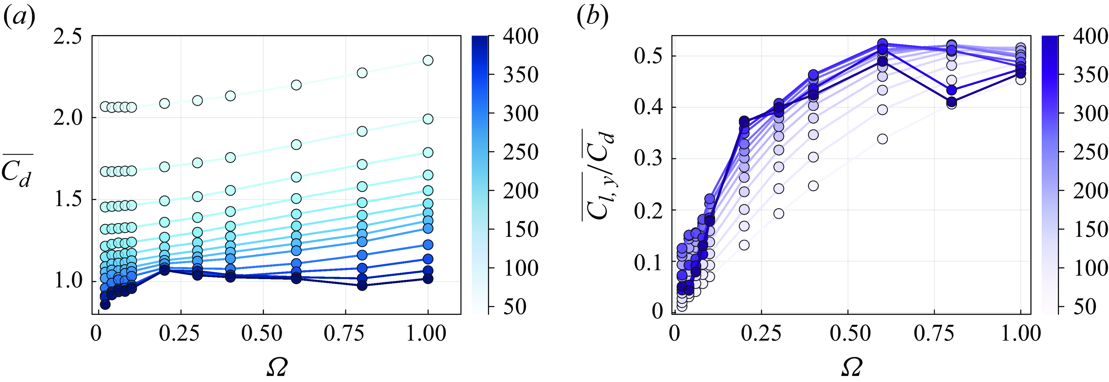
Figure 12. (a) Evolution of the time-averaged drag coefficient $\overline {C_d}$
of the rotating RCF4 cube as a function of
$\overline {C_d}$
of the rotating RCF4 cube as a function of $\Omega$
at
$\Omega$
at $40 \leqslant {{R}e} \leqslant 400$
. The increasing darkness of the circles represents higher flow inertia. (b) Evolution of the lift-to-drag ratio,
$40 \leqslant {{R}e} \leqslant 400$
. The increasing darkness of the circles represents higher flow inertia. (b) Evolution of the lift-to-drag ratio, $\overline {C_{l,y}}/\overline {C_d}$
, as a function of
$\overline {C_{l,y}}/\overline {C_d}$
, as a function of $\Omega$
at
$\Omega$
at $40 \leqslant {{R}e} \leqslant 400$
. The increasing darkness of the circles represents higher
$40 \leqslant {{R}e} \leqslant 400$
. The increasing darkness of the circles represents higher ${R}e$
.
${R}e$
.
Knowing the behaviour of both $\overline {C_{l,y}}$
and
$\overline {C_{l,y}}$
and $\overline {C_d}$
, we now plot the ratio of these two coefficients,
$\overline {C_d}$
, we now plot the ratio of these two coefficients, $\overline {C_{l,y}}/\overline {C_d}$
, in figure 12(b) to gain further insights into the hydrodynamic forces. A general trend is that the ratio
$\overline {C_{l,y}}/\overline {C_d}$
, in figure 12(b) to gain further insights into the hydrodynamic forces. A general trend is that the ratio $\overline {C_{l,y}}/\overline {C_d}$
increases with
$\overline {C_{l,y}}/\overline {C_d}$
increases with $\Omega$
. The effects of flow inertia tend to increase the ratio
$\Omega$
. The effects of flow inertia tend to increase the ratio $\overline {C_{l,y}}/\overline {C_d}$
, particularly for
$\overline {C_{l,y}}/\overline {C_d}$
, particularly for ${{R}e} \leqslant 200$
. However, at
${{R}e} \leqslant 200$
. However, at ${{R}e} \geqslant 250$
, the flow inertia has the opposite effect, decreasing this ratio. We know that the flow inertia and the particle rotation are competing factors in vortex generation. For
${{R}e} \geqslant 250$
, the flow inertia has the opposite effect, decreasing this ratio. We know that the flow inertia and the particle rotation are competing factors in vortex generation. For ${{R}e} \geqslant 250$
, the increasing flow inertia strengthens the vortex pairs on both the upper and lower surfaces of the rotating cube. This enhanced vortex activity moderates the strong lift forces generated by the Magnus effect, preventing further amplification of Magnus-induced lift and stabilising
${{R}e} \geqslant 250$
, the increasing flow inertia strengthens the vortex pairs on both the upper and lower surfaces of the rotating cube. This enhanced vortex activity moderates the strong lift forces generated by the Magnus effect, preventing further amplification of Magnus-induced lift and stabilising $\overline {C_{l,y}}/\overline {C_d}$
. The moderating effect of
$\overline {C_{l,y}}/\overline {C_d}$
. The moderating effect of ${R}e$
on the ratio is particularly pronounced in both slow rotation (
${R}e$
on the ratio is particularly pronounced in both slow rotation ( $0.02 \leftarrow \Omega$
) and fast rotation cases (
$0.02 \leftarrow \Omega$
) and fast rotation cases ( $\Omega \rightarrow 1$
). One exception is the region of drag insensitivity at
$\Omega \rightarrow 1$
). One exception is the region of drag insensitivity at $\Omega =0.2$
for
$\Omega =0.2$
for $250 \leqslant {{R}e} \leqslant 400$
, where we see the
$250 \leqslant {{R}e} \leqslant 400$
, where we see the $\overline {C_{l,y}}/\overline {C_d}$
keeps increasing with
$\overline {C_{l,y}}/\overline {C_d}$
keeps increasing with ${R}e$
. It is important to highlight that in all the cases investigated,
${R}e$
. It is important to highlight that in all the cases investigated, $\overline {C_{l,y}}/\overline {C_d}$
remains consistently bounded below
$\overline {C_{l,y}}/\overline {C_d}$
remains consistently bounded below $0.6$
, as depicted in figure 12(b). With increasing
$0.6$
, as depicted in figure 12(b). With increasing $\Omega$
,
$\Omega$
, $\overline {C_{l,y}}/\overline {C_d}$
does not increase monotonically, but instead reaches a plateau, as the flow dynamics at high rotation rates restrain further amplification of lift relative to drag.
$\overline {C_{l,y}}/\overline {C_d}$
does not increase monotonically, but instead reaches a plateau, as the flow dynamics at high rotation rates restrain further amplification of lift relative to drag.
4.4.3. Rotation coefficient
Given the significant impact of $\Omega$
and
$\Omega$
and ${R}e$
on the Magnus effect, we calculate the rotation coefficient, using (2.8), to quantify how effectively the rotation rate contributes to generating lift. A higher
${R}e$
on the Magnus effect, we calculate the rotation coefficient, using (2.8), to quantify how effectively the rotation rate contributes to generating lift. A higher $\overline {C_{\Omega }}$
indicates a greater efficiency of Magnus effect for a given
$\overline {C_{\Omega }}$
indicates a greater efficiency of Magnus effect for a given $\Omega$
. In figure 13, we show the evolution of the time-averaged rotation coefficient
$\Omega$
. In figure 13, we show the evolution of the time-averaged rotation coefficient $\overline {C_{\Omega }}$
as a function of
$\overline {C_{\Omega }}$
as a function of $\Omega$
, with marker darkness increasing with
$\Omega$
, with marker darkness increasing with ${R}e$
.
${R}e$
.
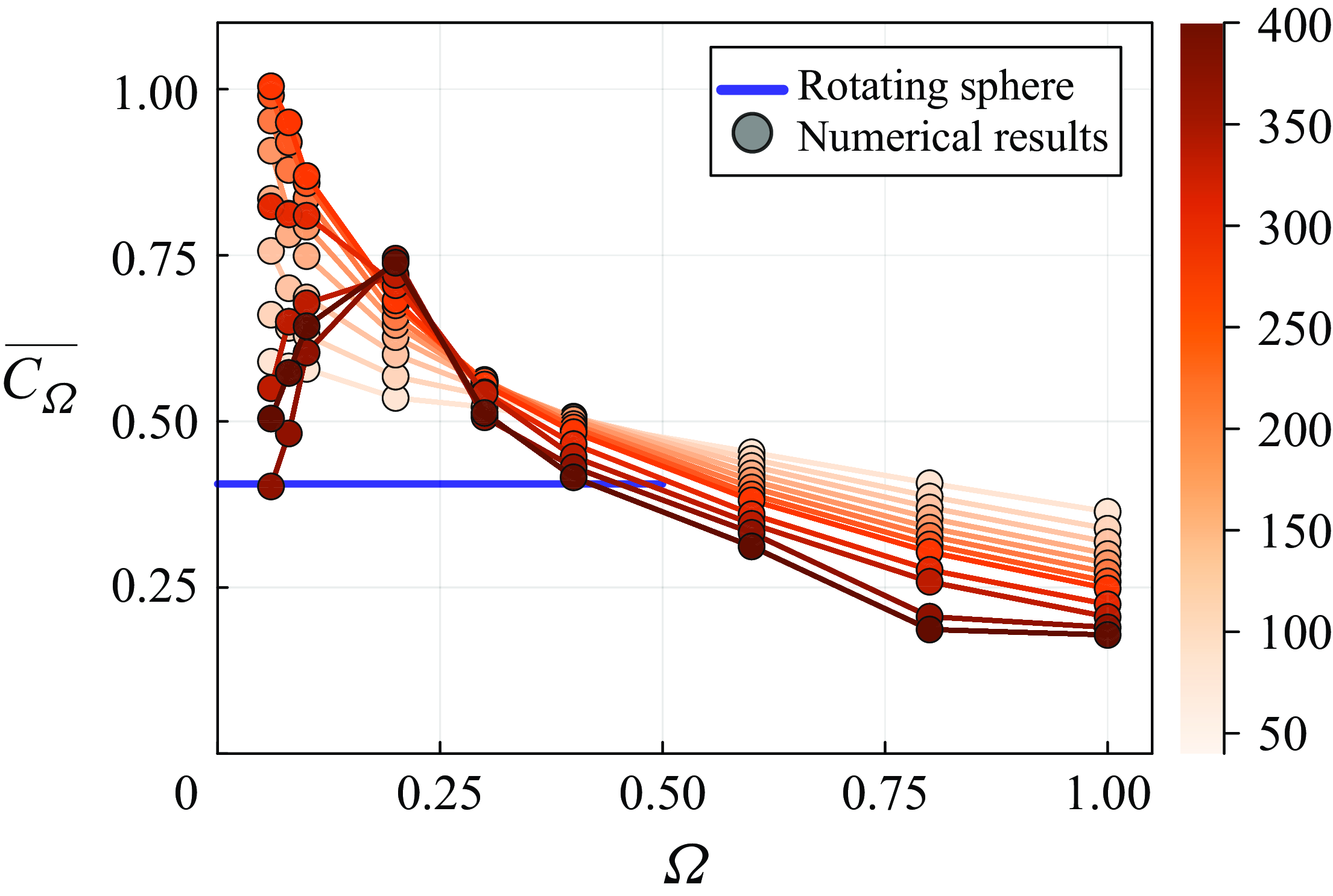
Figure 13. Evolution of the time-averaged rotation coefficient $\overline {C_\Omega }$
of the rotating RCF4 cube as a function of
$\overline {C_\Omega }$
of the rotating RCF4 cube as a function of $0.06 \leqslant \Omega \leqslant 1$
at
$0.06 \leqslant \Omega \leqslant 1$
at $40 \leqslant {{R}e} \leqslant 400$
. The increasing darkness of the circles represents higher
$40 \leqslant {{R}e} \leqslant 400$
. The increasing darkness of the circles represents higher ${R}e$
. The rotation coefficient of a rotating sphere,
${R}e$
. The rotation coefficient of a rotating sphere, $C_{\Omega , S} = 0.41$
, is marked by a blue horizontal line for
$C_{\Omega , S} = 0.41$
, is marked by a blue horizontal line for $\Omega \leqslant 0.5$
, as reported by Clanet (Reference Clanet2015), providing a comparative reference.
$\Omega \leqslant 0.5$
, as reported by Clanet (Reference Clanet2015), providing a comparative reference.
We observe that the efficiency of lift generation via the Magnus effect decreases monotonically with increasing $\Omega$
for low flow inertia cases
$\Omega$
for low flow inertia cases ${{R}e} \leqslant 200$
. For example, at
${{R}e} \leqslant 200$
. For example, at ${{R}e}=40$
,
${{R}e}=40$
, $\overline {C_{\Omega }}$
drops from
$\overline {C_{\Omega }}$
drops from $0.55$
at
$0.55$
at $\Omega =0.06$
to
$\Omega =0.06$
to $0.4$
at
$0.4$
at $\Omega =1$
, indicating that the flow becomes less responsive to rotation. The effects of increasing
$\Omega =1$
, indicating that the flow becomes less responsive to rotation. The effects of increasing ${R}e$
on
${R}e$
on $\overline {C_{\Omega }}$
are twofold. For
$\overline {C_{\Omega }}$
are twofold. For $\Omega \leqslant 0.2$
, higher flow inertia enhances the interaction between the rotating cube and the fluid, strengthening the Magnus effect. However, for faster-rotating cubes at
$\Omega \leqslant 0.2$
, higher flow inertia enhances the interaction between the rotating cube and the fluid, strengthening the Magnus effect. However, for faster-rotating cubes at $\Omega \geqslant 0.3$
, increasing
$\Omega \geqslant 0.3$
, increasing ${R}e$
reduces
${R}e$
reduces $\overline {C_{\Omega }}$
, as the enhanced flow unsteadiness decreases the pressure difference between the top and bottom of the particle, diminishing lift generation. As shown in figure 11, the decline in
$\overline {C_{\Omega }}$
, as the enhanced flow unsteadiness decreases the pressure difference between the top and bottom of the particle, diminishing lift generation. As shown in figure 11, the decline in $\overline {C_{l,y}}$
with
$\overline {C_{l,y}}$
with ${R}e$
at
${R}e$
at $\Omega \geqslant 0.4$
is a direct result of the diminished efficiency of the Magnus effect. At higher flow inertia,
$\Omega \geqslant 0.4$
is a direct result of the diminished efficiency of the Magnus effect. At higher flow inertia, ${{R}e} \geqslant 250$
,
${{R}e} \geqslant 250$
, $\overline {C_{\Omega }}$
generally decreases, except at
$\overline {C_{\Omega }}$
generally decreases, except at $\Omega = 0.2$
. At low rotation rates,
$\Omega = 0.2$
. At low rotation rates, $\Omega \leqslant 0.1$
, increasing
$\Omega \leqslant 0.1$
, increasing ${R}e$
reduces lift due to chaotic shedding, which disrupts vortex distribution and diminishes the lift force. However, at
${R}e$
reduces lift due to chaotic shedding, which disrupts vortex distribution and diminishes the lift force. However, at $\Omega = 0.2$
,
$\Omega = 0.2$
, $\overline {C_{\Omega }}$
shows a distinct trend, continuing to increase across the entire Reynolds number range
$\overline {C_{\Omega }}$
shows a distinct trend, continuing to increase across the entire Reynolds number range $40 \leqslant {{R}e} \leqslant 400$
, indicating enhanced rotational efficiency. This behaviour is closely linked to the reorganisation of vortex pairs and their high shedding frequency at
$40 \leqslant {{R}e} \leqslant 400$
, indicating enhanced rotational efficiency. This behaviour is closely linked to the reorganisation of vortex pairs and their high shedding frequency at $\Omega = 0.2$
. A comparison is made with the characteristic rotation coefficient of a sphere
$\Omega = 0.2$
. A comparison is made with the characteristic rotation coefficient of a sphere $C_{\Omega , S} = 0.41$
for
$C_{\Omega , S} = 0.41$
for $\Omega \leqslant 0.5$
(Clanet Reference Clanet2015). The blue horizontal line in figure 13 serves as a reference to compare the rotating cube with a sphere under similar conditions. The cube demonstrates higher rotational efficiency, particularly at lower rotation rates, indicating a stronger Magnus effect due to its sharp edges. Analogous to the empirical correlation for
$\Omega \leqslant 0.5$
(Clanet Reference Clanet2015). The blue horizontal line in figure 13 serves as a reference to compare the rotating cube with a sphere under similar conditions. The cube demonstrates higher rotational efficiency, particularly at lower rotation rates, indicating a stronger Magnus effect due to its sharp edges. Analogous to the empirical correlation for $\overline {C_{l,y}}$
, we propose an equally valuable correlation for
$\overline {C_{l,y}}$
, we propose an equally valuable correlation for $\overline {C_{\Omega }}$
at
$\overline {C_{\Omega }}$
at $40 \leqslant {{R}e} \leqslant 200$
in (E2) (see Appendix E).
$40 \leqslant {{R}e} \leqslant 200$
in (E2) (see Appendix E).
From a broader perspective, the force coefficients ( $\overline {C_d}$
,
$\overline {C_d}$
, $\overline {C_{l,y}}$
and
$\overline {C_{l,y}}$
and $\overline {C_{\Omega }}$
) of the RCF4 provide essential insights on trajectories of settling angular particles. In our prior work (Gai & Wachs Reference Gai and Wachs2024), we demonstrated that the Magnus force and hydrodynamic torque play significant roles in shaping the trajectory of a freely settling cube, sustaining an intriguing helical motion in the HS regime. The Magnus force serves as the primary driver of the cube horizontal motion. Then, the resulting rotation-induced drift generates a secondary Magnus force that amplifies the settling drag. It is also demonstrated that the enhanced hydrodynamic torque triggers the transition from the oblique to the helical settling regimes. An additional analysis of the hydrodynamic torque
$\overline {C_{\Omega }}$
) of the RCF4 provide essential insights on trajectories of settling angular particles. In our prior work (Gai & Wachs Reference Gai and Wachs2024), we demonstrated that the Magnus force and hydrodynamic torque play significant roles in shaping the trajectory of a freely settling cube, sustaining an intriguing helical motion in the HS regime. The Magnus force serves as the primary driver of the cube horizontal motion. Then, the resulting rotation-induced drift generates a secondary Magnus force that amplifies the settling drag. It is also demonstrated that the enhanced hydrodynamic torque triggers the transition from the oblique to the helical settling regimes. An additional analysis of the hydrodynamic torque $\overline {T_z}$
is presented in Appendix F, where we propose a simple scaling law to model
$\overline {T_z}$
is presented in Appendix F, where we propose a simple scaling law to model $\overline {T_z}$
of the RCF4 over the range
$\overline {T_z}$
of the RCF4 over the range $200 \leqslant {{R}e} \leqslant 400$
, yielding a correlation with an
$200 \leqslant {{R}e} \leqslant 400$
, yielding a correlation with an $r^2=0.999$
.
$r^2=0.999$
.
In previous studies, the absence of accurate correlations necessitated the use of approximate values in force balance analysis to gain insight into the underlying physics. By providing more accurate lift, drag and torque coefficients, and correlations for a centre-fixed rotating cube, we offer an approach to overcome this limitation, paving the way for more robust and physically grounded analyses in future research.
4.5. Vortex shedding frequency
While time-averaged drag and lift forces serve as essential design and engineering metrics, understanding the unsteady fluctuations and their frequencies is crucial for analysing particle trajectory instabilities, mixing and collision dynamics. Figures 8–10 reveal that the flow past a rotating cube displays a variety of vortex shedding patterns. The shedding frequency increases with rising $\Omega$
, before stabilising in the VS and KH regimes. To clarify how the vortex shedding frequencies evolve with
$\Omega$
, before stabilising in the VS and KH regimes. To clarify how the vortex shedding frequencies evolve with $\Omega$
, we apply fast Fourier transform (FFT) to the temporal evolution of the lift force, resulting in the frequency spectra presented in figure 14. Three Reynolds numbers (
$\Omega$
, we apply fast Fourier transform (FFT) to the temporal evolution of the lift force, resulting in the frequency spectra presented in figure 14. Three Reynolds numbers ( ${{R}e} = 80$
,
${{R}e} = 80$
, $ 160$
and
$ 160$
and $ 400$
) are selected as representative examples of low, moderate and high flow inertia. Each subpanel shows the frequency spectrum (solid blue lines) from
$ 400$
) are selected as representative examples of low, moderate and high flow inertia. Each subpanel shows the frequency spectrum (solid blue lines) from $\Omega = 0.02$
to
$\Omega = 0.02$
to $\Omega = 1$
, with the frequency of the primary peak annotated next to it. We report in each subpanel the rotation rate
$\Omega = 1$
, with the frequency of the primary peak annotated next to it. We report in each subpanel the rotation rate $\Omega$
as a red dashed line in addition to reporting its value in the top right corner. As reference points, we also plot two characteristic frequencies of the flow past a fixed cube: (i) the vortex shedding frequency, i.e. the primary peak, as yellow dashed lines and (ii) the first harmonic of the primary peak as grey dashed lines (Gai & Wachs Reference Gai and Wachs2023b
).
$\Omega$
as a red dashed line in addition to reporting its value in the top right corner. As reference points, we also plot two characteristic frequencies of the flow past a fixed cube: (i) the vortex shedding frequency, i.e. the primary peak, as yellow dashed lines and (ii) the first harmonic of the primary peak as grey dashed lines (Gai & Wachs Reference Gai and Wachs2023b
).
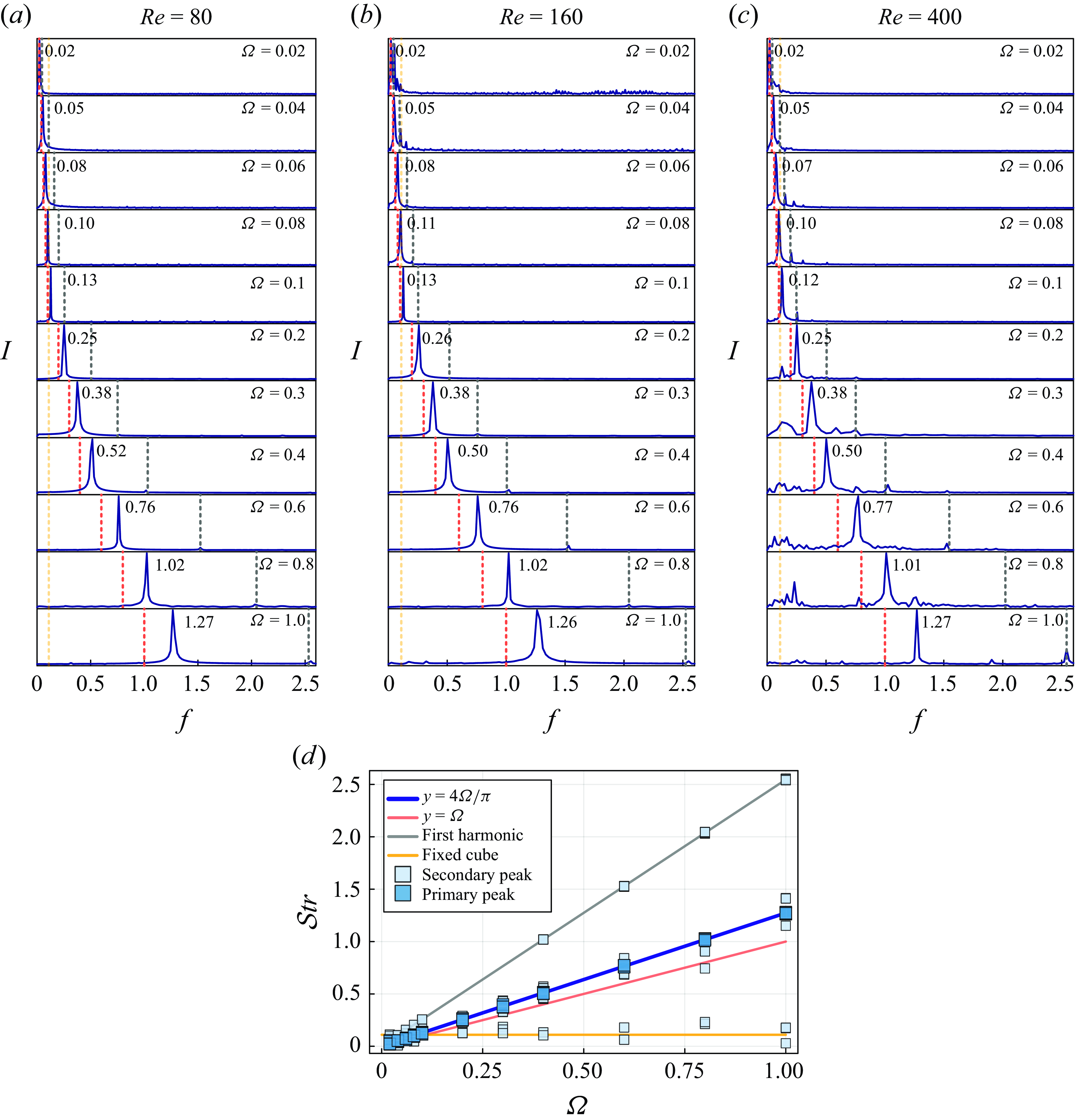
Figure 14. (a–c) Vortex shedding frequency $f$
spectrum of the rotating RCF4 cube at
$f$
spectrum of the rotating RCF4 cube at ${{R}e} = 80, 160$
and
${{R}e} = 80, 160$
and $400$
.
$400$
. $I$
represents the frequency intensity obtained via FFT and is displayed on a linear scale in each panel. (d) Strouhal number
$I$
represents the frequency intensity obtained via FFT and is displayed on a linear scale in each panel. (d) Strouhal number $\mathcal{S}\textit{tr}$
of the primary and secondary peaks as a function of
$\mathcal{S}\textit{tr}$
of the primary and secondary peaks as a function of $\Omega$
for all values of
$\Omega$
for all values of $\Omega$
and
$\Omega$
and ${R}e$
considered. The blue curve represents the fitting for the primary peak
${R}e$
considered. The blue curve represents the fitting for the primary peak $\mathcal{S}\textit{tr}_1$
, following
$\mathcal{S}\textit{tr}_1$
, following $y=4\Omega /\pi$
, while the red curve shows the imposed rotation rate,
$y=4\Omega /\pi$
, while the red curve shows the imposed rotation rate, $y=\Omega$
. The grey curve indicates the first harmonic of the primary peak frequency, and the yellow curve corresponds to the characteristic
$y=\Omega$
. The grey curve indicates the first harmonic of the primary peak frequency, and the yellow curve corresponds to the characteristic $\mathcal{S}\textit{tr}_0=0.11$
of the flow past a fixed cube (Gai & Wachs Reference Gai and Wachs2023b
). Dashed lines in the corresponding colours are reported in panel (a–c) in each case.
$\mathcal{S}\textit{tr}_0=0.11$
of the flow past a fixed cube (Gai & Wachs Reference Gai and Wachs2023b
). Dashed lines in the corresponding colours are reported in panel (a–c) in each case.
At ${{R}e} = 80$
, the frequency spectrum shows a single dominant peak across all rotation rates
${{R}e} = 80$
, the frequency spectrum shows a single dominant peak across all rotation rates $0.02 \leqslant \Omega \leqslant 1$
, with values increasing proportionally to
$0.02 \leqslant \Omega \leqslant 1$
, with values increasing proportionally to $\Omega$
. As shown in figure 23, at low flow inertia, the wake vortical structures using
$\Omega$
. As shown in figure 23, at low flow inertia, the wake vortical structures using $\lambda _2=-1$
remain steady or fragmented within the SV, UV and VS regimes. Vortex shedding occurs only at
$\lambda _2=-1$
remain steady or fragmented within the SV, UV and VS regimes. Vortex shedding occurs only at $\Omega = 0.1$
and
$\Omega = 0.1$
and $\Omega = 0.2$
in the HS regime at
$\Omega = 0.2$
in the HS regime at ${{R}e} = 80$
. The dominant frequency seen in the blue curves in figure 14(a) corresponds to the generation and shedding of the upper and lower streamwise vortex pairs, as illustrated in figure 9. The lower panel of figure 9 shows that each effective face of the rotating cube produces one pair of upper vortices and one pair of lower vortices. Consequently, for a rotating cube with a four-fold axis, four pairs of upper/lower streamwise vortices are generated during a complete rotation cycle. At higher flow inertia,
${{R}e} = 80$
. The dominant frequency seen in the blue curves in figure 14(a) corresponds to the generation and shedding of the upper and lower streamwise vortex pairs, as illustrated in figure 9. The lower panel of figure 9 shows that each effective face of the rotating cube produces one pair of upper vortices and one pair of lower vortices. Consequently, for a rotating cube with a four-fold axis, four pairs of upper/lower streamwise vortices are generated during a complete rotation cycle. At higher flow inertia, ${{R}e} = 160$
, the primary peak values in figure 14(b) remain nearly identical to those at
${{R}e} = 160$
, the primary peak values in figure 14(b) remain nearly identical to those at ${{R}e} = 80$
, despite differences in the flow regime transition sequence. For
${{R}e} = 80$
, despite differences in the flow regime transition sequence. For $\Omega \geqslant 0.3$
, a small secondary peak emerges as the first harmonic frequency, likely due to nonlinear effects such as intricate vortex interactions or flow instabilities. At
$\Omega \geqslant 0.3$
, a small secondary peak emerges as the first harmonic frequency, likely due to nonlinear effects such as intricate vortex interactions or flow instabilities. At ${{R}e} = 400$
, while the primary peak is still similar to those at lower Reynolds numbers, the first harmonic becomes significantly more pronounced. Interestingly, a distinct high-intensity region appears near the characteristic vortex shedding frequency for a fixed cube,
${{R}e} = 400$
, while the primary peak is still similar to those at lower Reynolds numbers, the first harmonic becomes significantly more pronounced. Interestingly, a distinct high-intensity region appears near the characteristic vortex shedding frequency for a fixed cube, $\mathcal{S}\textit{tr}_0 = 0.11$
. Between
$\mathcal{S}\textit{tr}_0 = 0.11$
. Between $\Omega = 0.3$
and
$\Omega = 0.3$
and $\Omega = 0.8$
, the high-value plateau around
$\Omega = 0.8$
, the high-value plateau around $\mathcal{S}\textit{tr}_0 = 0.11$
stands out, reflecting the persistent obstacle effect of the cube in the flow, independent of its rotation.
$\mathcal{S}\textit{tr}_0 = 0.11$
stands out, reflecting the persistent obstacle effect of the cube in the flow, independent of its rotation.
To capture the overall behaviour of the shedding frequency, we apply FFT to all cases investigated and compute $\mathcal{S}\textit{tr}$
using (2.9). The results are plotted as a function of
$\mathcal{S}\textit{tr}$
using (2.9). The results are plotted as a function of $\Omega$
in figure 14(d). The dark and light blue square markers represent the Strouhal numbers based on the primary peak (
$\Omega$
in figure 14(d). The dark and light blue square markers represent the Strouhal numbers based on the primary peak ( $\mathcal{S}\textit{tr}_1$
) and the secondary peak (
$\mathcal{S}\textit{tr}_1$
) and the secondary peak ( $\mathcal{S}\textit{tr}_2$
), respectively. By applying linear regression to the evolution of
$\mathcal{S}\textit{tr}_2$
), respectively. By applying linear regression to the evolution of $\mathcal{S}\textit{tr}_1$
with
$\mathcal{S}\textit{tr}_1$
with $\Omega$
, we derive the following relationship:
$\Omega$
, we derive the following relationship:
 \begin{equation} \mathcal{S}\textit{tr}_1 = \frac {4}{\pi }\Omega \end{equation}
with a coefficient of determination $R^2 = 0.99$
. The fitting curve is represented by the navy solid line in figure 14(d). This equation describes the shedding frequency of the streamwise vortex pairs on the particle surface, and is therefore closely correlated with both the rotation rate
$R^2 = 0.99$
. The fitting curve is represented by the navy solid line in figure 14(d). This equation describes the shedding frequency of the streamwise vortex pairs on the particle surface, and is therefore closely correlated with both the rotation rate $\Omega$
and the rotational symmetry fold (
$\Omega$
and the rotational symmetry fold ( $n_{\Omega }=4$
for RCF4).
$n_{\Omega }=4$
for RCF4).
In figure 14(d), the secondary peaks $\mathcal{S}\textit{tr}_2$
from all
$\mathcal{S}\textit{tr}_2$
from all $143$
simulations of RCF4 can be clearly categorised into three distinct groups: (i) those adjacent to the primary peak, representing the shedding of vortex pairs from the cube surface; (ii) those along the curve of the first harmonics (grey solid line), reflecting more intricate vortex interactions; and (iii) those near the fixed cube frequency
$143$
simulations of RCF4 can be clearly categorised into three distinct groups: (i) those adjacent to the primary peak, representing the shedding of vortex pairs from the cube surface; (ii) those along the curve of the first harmonics (grey solid line), reflecting more intricate vortex interactions; and (iii) those near the fixed cube frequency $\mathcal{S}\textit{tr}_0 = 0.11$
(orange horizontal line), which corresponds to the obstacle effect of the cube without rotation. In general, increasing flow inertia amplifies the intensity of the first harmonics. For flows with low inertia,
$\mathcal{S}\textit{tr}_0 = 0.11$
(orange horizontal line), which corresponds to the obstacle effect of the cube without rotation. In general, increasing flow inertia amplifies the intensity of the first harmonics. For flows with low inertia, ${{R}e} \leqslant 200$
, the wake structure shedding frequency, identified using the
${{R}e} \leqslant 200$
, the wake structure shedding frequency, identified using the $\lambda = -1$
criterion, is primarily dominated by
$\lambda = -1$
criterion, is primarily dominated by $\mathcal{S}\textit{tr}_1$
for
$\mathcal{S}\textit{tr}_1$
for $\Omega \leqslant 0.2$
, as shown in figure 8(a). In the KH regime, the shedding of wake vortices caused by K-H instabilities occurs farther from the rear surface of the particle, making them difficult to observe directly in figure 14. At higher flow inertia, as seen in figure 10, the obstacle effect of the cube becomes dominant in the CS regime. Their wake structure shedding frequency is predominantly governed by
$\Omega \leqslant 0.2$
, as shown in figure 8(a). In the KH regime, the shedding of wake vortices caused by K-H instabilities occurs farther from the rear surface of the particle, making them difficult to observe directly in figure 14. At higher flow inertia, as seen in figure 10, the obstacle effect of the cube becomes dominant in the CS regime. Their wake structure shedding frequency is predominantly governed by $\mathcal{S}\textit{tr}_2 \approx 0.11$
, closely aligned with the orange curve in figure 14(d). Additional vortex shedding patterns are presented in Appendix C for further reference.
$\mathcal{S}\textit{tr}_2 \approx 0.11$
, closely aligned with the orange curve in figure 14(d). Additional vortex shedding patterns are presented in Appendix C for further reference.
5. Extending insights to general angular particles
In this section, we extend our analysis from the cube to other rotating angular particles to further investigate the impact of particle shape on the Magnus effect and wake instability. A key challenge in studying angular particles is the infinite number of possible angular positions, particularly when the particle is rotating. To address this, we focus on the rotation axis of the particle and explore how the number of rotational symmetry folds $n_{\Omega }$
affects the vortex shedding and its suppression, offering insights into the relationship between particle geometry and wake instability.
$n_{\Omega }$
affects the vortex shedding and its suppression, offering insights into the relationship between particle geometry and wake instability.
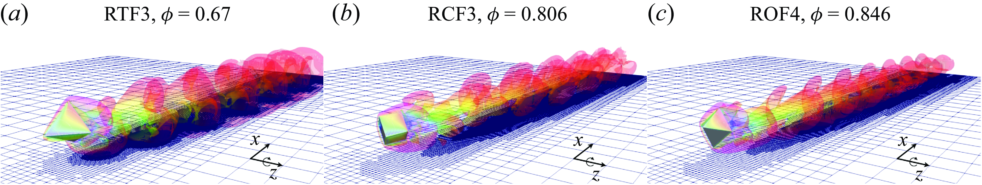
Figure 15. Configuration of the flow past a transversely rotating angular particle at ${{R}e}=100$
and
${{R}e}=100$
and $\Omega =0.2$
with rotation axis along the
$\Omega =0.2$
with rotation axis along the $z$
-direction, illustrating wake vortex structures identified by
$z$
-direction, illustrating wake vortex structures identified by $\lambda _2 = -1$
, coloured by the streamwise velocity
$\lambda _2 = -1$
, coloured by the streamwise velocity $u_x$
(red for high velocity and blue for low velocity). (a) Rotating RTF3 tetrahedron with a three-fold axis, (b) rotating RCF3 cube with a three-fold axis and (c) rotating ROF4 octahedron with a four-fold axis.
$u_x$
(red for high velocity and blue for low velocity). (a) Rotating RTF3 tetrahedron with a three-fold axis, (b) rotating RCF3 cube with a three-fold axis and (c) rotating ROF4 octahedron with a four-fold axis.
In addition to the four-fold rotating cube (RCF4) discussed earlier, we examine three angular particles: a tetrahedron (three-fold, RTF3), another cube (three-fold, RCF3) and an octahedron (four-fold, ROF4), with their rotation axis illustrated in figure 2. We recall that $n_{\Omega }$
refers to the number of times an angular particle can be rotated by equal angles around the axis while retaining an identical appearance. To provide a clearer visualisation of their rotation in the computational domain, figure 15 presents the flow configurations in the three additional cases. At the same
$n_{\Omega }$
refers to the number of times an angular particle can be rotated by equal angles around the axis while retaining an identical appearance. To provide a clearer visualisation of their rotation in the computational domain, figure 15 presents the flow configurations in the three additional cases. At the same ${R}e$
and
${R}e$
and $\Omega$
, the wake structures vary significantly depending on both the particle angularity
$\Omega$
, the wake structures vary significantly depending on both the particle angularity $\phi$
and
$\phi$
and $n_{\Omega }$
. We perform 99 additional numerical simulations of the flow past these three angular particles, covering
$n_{\Omega }$
. We perform 99 additional numerical simulations of the flow past these three angular particles, covering ${{R}e} = 60$
,
${{R}e} = 60$
, $100$
and
$100$
and $160$
, and a range of
$160$
, and a range of $0.02 \leqslant \Omega \leqslant 1$
.
$0.02 \leqslant \Omega \leqslant 1$
.
5.1. Influence of the number of rotational symmetry folds on flow regimes and wake instability
For a comprehensive view of the effects of particle shape and $n_{\Omega }$
on flow regime transitions, we present the regime map for flows past transversely rotating angular particles at
$n_{\Omega }$
on flow regime transitions, we present the regime map for flows past transversely rotating angular particles at $60 \leqslant {{R}e} \leqslant 160$
in figure 16. The lower subpanel compares the two angular particles with
$60 \leqslant {{R}e} \leqslant 160$
in figure 16. The lower subpanel compares the two angular particles with $n_{\Omega }=3$
, specifically RCF3 and RTF3, while the upper subpanel focuses on the particles with
$n_{\Omega }=3$
, specifically RCF3 and RTF3, while the upper subpanel focuses on the particles with $n_{\Omega }=4$
. The regimes of the RCF4 are included for comparison with the ROF4. For consistency, the same colour scheme as that used in the regime map in figure 4 is used. Within the selected range of
$n_{\Omega }=4$
. The regimes of the RCF4 are included for comparison with the ROF4. For consistency, the same colour scheme as that used in the regime map in figure 4 is used. Within the selected range of ${R}e$
, figure 16 illustrates the transition sequence, starting from the SV regime to vortex shedding in the HS regime, followed by vortex suppression in the VS and KH regimes.
${R}e$
, figure 16 illustrates the transition sequence, starting from the SV regime to vortex shedding in the HS regime, followed by vortex suppression in the VS and KH regimes.
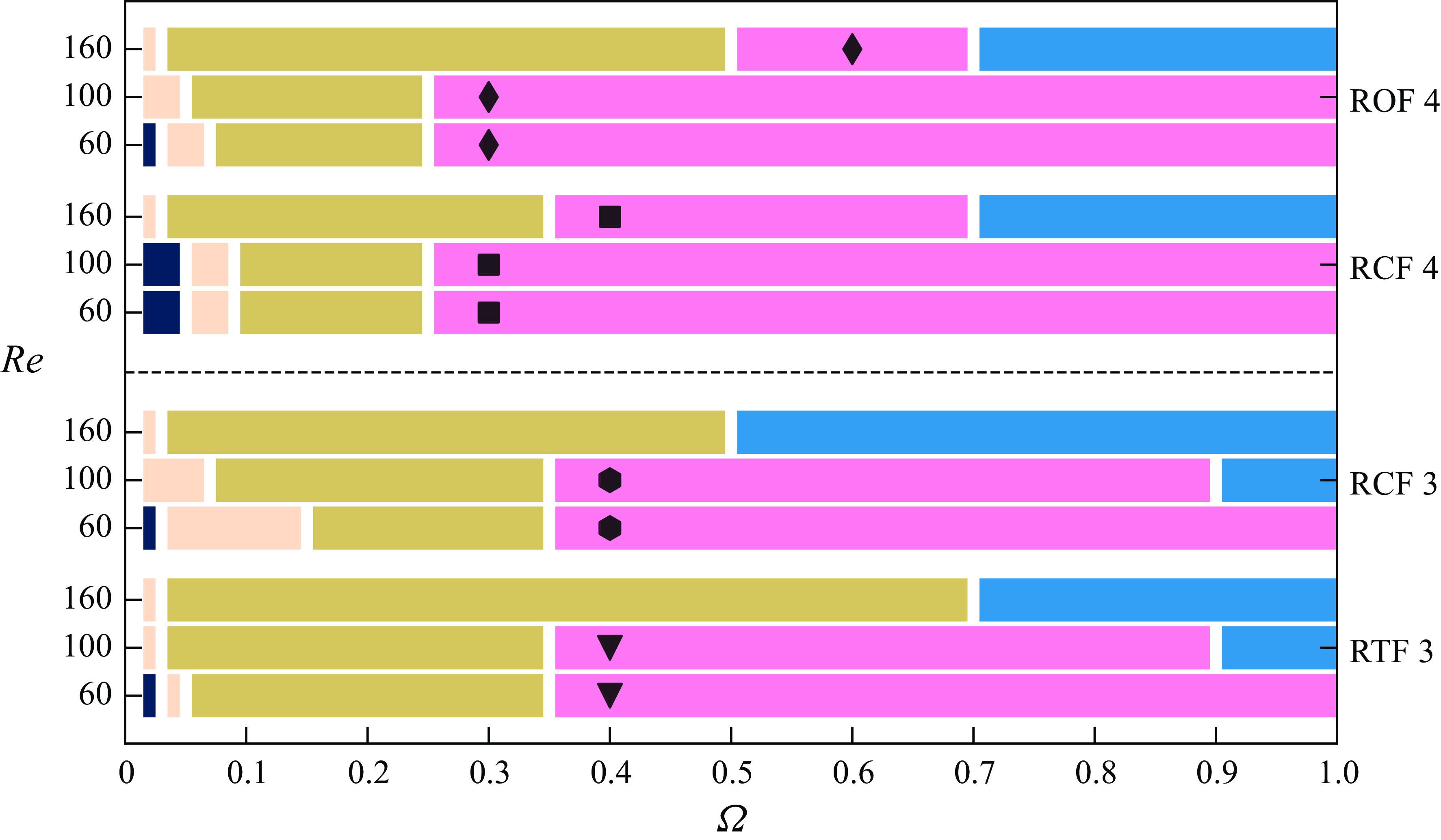
Figure 16. Regime transitions of the flow past a rotating angular particle at ${{R}e}=60,100$
and
${{R}e}=60,100$
and $160$
for
$160$
for $0.02 \leqslant \Omega \leqslant 1$
. Onset of vortex suppression for RTF3 (
$0.02 \leqslant \Omega \leqslant 1$
. Onset of vortex suppression for RTF3 (
![]() ), RCF3 (
), RCF3 (
![]() ), RCF4 (
), RCF4 (
![]() ) and ROF4 (
) and ROF4 (
![]() ).
).
A key observation from figure 16 is that $n_{\Omega }$
plays a dominant role in regime transitions. For the three-fold cases, RTF3 and RCF3 exhibit highly similar transition sequences, as shown in the lower subpanel. Vortex suppression begins at the same rotation rate,
$n_{\Omega }$
plays a dominant role in regime transitions. For the three-fold cases, RTF3 and RCF3 exhibit highly similar transition sequences, as shown in the lower subpanel. Vortex suppression begins at the same rotation rate, $\Omega = 0.4$
, for both
$\Omega = 0.4$
, for both ${{R}e} = 60$
and
${{R}e} = 60$
and $100$
. The KH regime replaces the VS regime at
$100$
. The KH regime replaces the VS regime at ${{R}e} = 160$
in both cases. In the four-fold cases, vortex suppression occurs at a lower rotation rate,
${{R}e} = 160$
in both cases. In the four-fold cases, vortex suppression occurs at a lower rotation rate, $\Omega = 0.3$
, for both RCF4 and ROF4 at
$\Omega = 0.3$
, for both RCF4 and ROF4 at ${{R}e} = 60$
and
${{R}e} = 60$
and $100$
. A slight difference emerges at
$100$
. A slight difference emerges at ${{R}e} = 160$
, where vortex suppression for ROF4 occurs at a higher
${{R}e} = 160$
, where vortex suppression for ROF4 occurs at a higher $\Omega$
compared with RCF4. Overall, the regime transition for RCF4 shows strong similarities with the regime transition for ROF4.
$\Omega$
compared with RCF4. Overall, the regime transition for RCF4 shows strong similarities with the regime transition for ROF4.
By comparing the upper and lower subpanels, we observe that increasing $n_{\Omega }$
leads to vortex suppression at a lower critical
$n_{\Omega }$
leads to vortex suppression at a lower critical $\Omega$
. Within the range of
$\Omega$
. Within the range of ${R}e$
discussed, particle rotation stabilises the wake structure through vortex merging, while flow inertia tends to induce instabilities. A higher
${R}e$
discussed, particle rotation stabilises the wake structure through vortex merging, while flow inertia tends to induce instabilities. A higher $n_{\Omega }$
enhances this stabilising effect, as seen in the four-fold cases where the VS regime persists at
$n_{\Omega }$
enhances this stabilising effect, as seen in the four-fold cases where the VS regime persists at ${{R}e} = 160$
. By contrast, in the three-fold cases, the VS regime is replaced by the KH regime at the same
${{R}e} = 160$
. By contrast, in the three-fold cases, the VS regime is replaced by the KH regime at the same ${R}e$
, as shown in the lower subpanel. Particle angularity
${R}e$
, as shown in the lower subpanel. Particle angularity $\phi$
has less impact than
$\phi$
has less impact than $n_{\Omega }$
on regime transitions. As illustrated in figure 16, RTF3 (
$n_{\Omega }$
on regime transitions. As illustrated in figure 16, RTF3 ( $\phi =0.67$
) begins vortex shedding at a lower rotation rate than the less angular RCF3 (
$\phi =0.67$
) begins vortex shedding at a lower rotation rate than the less angular RCF3 ( $\phi =0.806$
). However, this trend does not hold for the four-fold cases, as RCF4 (
$\phi =0.806$
). However, this trend does not hold for the four-fold cases, as RCF4 ( $\phi =0.806$
) and ROF4 (
$\phi =0.806$
) and ROF4 ( $\phi =0.846$
) exhibit the opposite behaviour.
$\phi =0.846$
) exhibit the opposite behaviour.
To elucidate the effects of $\phi$
and
$\phi$
and $n_{\Omega }$
on wake instabilities, figure 17 illustrates the wake structures for flows at
$n_{\Omega }$
on wake instabilities, figure 17 illustrates the wake structures for flows at ${{R}e} = 100$
with rotation rates in the range
${{R}e} = 100$
with rotation rates in the range $0.1 \leqslant \Omega \leqslant 0.4$
. We show a side view of the wake vortical structures for the three-fold angular particles RTF3 and RCF3 in figure 17(a). At
$0.1 \leqslant \Omega \leqslant 0.4$
. We show a side view of the wake vortical structures for the three-fold angular particles RTF3 and RCF3 in figure 17(a). At $\Omega = 0.1$
, RCF3 exhibits more fragmented vortex structures than RTF3, due to the higher number of effective faces
$\Omega = 0.1$
, RCF3 exhibits more fragmented vortex structures than RTF3, due to the higher number of effective faces $N_{\mathcal{F}}$
. In the flow configuration of figure 15(b), the three-fold cube RCF3 has six faces
$N_{\mathcal{F}}$
. In the flow configuration of figure 15(b), the three-fold cube RCF3 has six faces $N_{\mathcal{F}}=6$
contributing to vortex generation during rotation, while the three-fold tetrahedron RTF3 has only three
$N_{\mathcal{F}}=6$
contributing to vortex generation during rotation, while the three-fold tetrahedron RTF3 has only three $N_{\mathcal{F}}=3$
, as its fourth face is parallel to the flow and hardly impacts the wake. At
$N_{\mathcal{F}}=3$
, as its fourth face is parallel to the flow and hardly impacts the wake. At $\Omega \geqslant 0.2$
, the wake structures and shedding frequencies of RTF3 and RCF3 become more similar. Although some shape effects remain noticeable at
$\Omega \geqslant 0.2$
, the wake structures and shedding frequencies of RTF3 and RCF3 become more similar. Although some shape effects remain noticeable at $\Omega = 0.2$
, they diminish at
$\Omega = 0.2$
, they diminish at $\Omega = 0.3$
, and by
$\Omega = 0.3$
, and by $\Omega = 0.4$
, both RTF3 and RCF3 exhibit the same steady wake structures in the VS regime. In figure 17(b), the wake structures behind RCF4 and ROF4 exhibit a striking similarity in both topology and frequency, with minimal influence from angularity. Note that ROF4 features two faces per fold; however, since they are in phase, they operate as one single effective face per fold. Hence, ROF4 and RCF4 both have four effective faces per rotation period
$\Omega = 0.4$
, both RTF3 and RCF3 exhibit the same steady wake structures in the VS regime. In figure 17(b), the wake structures behind RCF4 and ROF4 exhibit a striking similarity in both topology and frequency, with minimal influence from angularity. Note that ROF4 features two faces per fold; however, since they are in phase, they operate as one single effective face per fold. Hence, ROF4 and RCF4 both have four effective faces per rotation period $N_{\mathcal{F}}=4$
. At
$N_{\mathcal{F}}=4$
. At $\Omega = 0.3$
, both particles exhibit clear signs of vortex suppression. Despite differences in shape and angularity, RCF4 and ROF4 behave almost identically, suggesting that
$\Omega = 0.3$
, both particles exhibit clear signs of vortex suppression. Despite differences in shape and angularity, RCF4 and ROF4 behave almost identically, suggesting that $n_{\Omega }$
is the key factor that controls wake dynamics.
$n_{\Omega }$
is the key factor that controls wake dynamics.
We further plot the isosurfaces of streamwise vortices $\omega _x = \pm 0.03$
in figure 17(c) to compare RTF3 and RCF3. The vortex generation on the surface of the tetrahedron differs significantly from that on the surface of the cube. In the RTF3 case at
$\omega _x = \pm 0.03$
in figure 17(c) to compare RTF3 and RCF3. The vortex generation on the surface of the tetrahedron differs significantly from that on the surface of the cube. In the RTF3 case at $\Omega = 0.1$
, an entwined structure of blue and red vortices is observed, while in the RCF3 case, the two opposite-signed vortices are more separated, positioned on either side of the horizontal centreline in the
$\Omega = 0.1$
, an entwined structure of blue and red vortices is observed, while in the RCF3 case, the two opposite-signed vortices are more separated, positioned on either side of the horizontal centreline in the $x$
-
$x$
- $z$
plane. This difference in vortex pair generation explains the variation in wake structures between RTF3 and RCF3. From
$z$
plane. This difference in vortex pair generation explains the variation in wake structures between RTF3 and RCF3. From $\Omega = 0.3$
to
$\Omega = 0.3$
to $\Omega = 0.4$
, we highlight the merging of three blue streamwise vortices into a single one, as indicated by the yellow arrow. The distribution of
$\Omega = 0.4$
, we highlight the merging of three blue streamwise vortices into a single one, as indicated by the yellow arrow. The distribution of $\omega _x$
in the
$\omega _x$
in the $y$
-
$y$
- $z$
plane in the particle wake shows that planar symmetry is already broken in these cases. However, by
$z$
plane in the particle wake shows that planar symmetry is already broken in these cases. However, by $\Omega = 0.4$
, the wake structure becomes steady as a result of vortex merging. Despite differences in vortex patterns between RTF3 and RCF3, the merging process remains consistent in both cases.
$\Omega = 0.4$
, the wake structure becomes steady as a result of vortex merging. Despite differences in vortex patterns between RTF3 and RCF3, the merging process remains consistent in both cases.
Similarly, figure 17(d) presents the isosurface of $\omega _x = \pm 0.03$
for RCF4 and ROF4. The distribution of
$\omega _x = \pm 0.03$
for RCF4 and ROF4. The distribution of $\omega _x$
in the
$\omega _x$
in the $y$
-
$y$
- $z$
plane at
$z$
plane at $x = x_p + 1.5$
is shown in the middle of the figure, with green lines indicating their position in the
$x = x_p + 1.5$
is shown in the middle of the figure, with green lines indicating their position in the $x$
-
$x$
- $z$
plane. Since RCF4 and ROF4 both have four effective faces during rotation, we observe highly symmetric vortex pairs in both the
$z$
plane. Since RCF4 and ROF4 both have four effective faces during rotation, we observe highly symmetric vortex pairs in both the $x$
-
$x$
- $z$
and
$z$
and $y$
-
$y$
- $z$
planes. For
$z$
planes. For $0.2 \leqslant \Omega \leqslant 0.3$
, the yellow arrow highlights the merging of three smaller blue vortices into a long blue tail in the ROF4 case. This indicates that vortex suppression occurs due to the merging of vortices of same sign, a process enhanced by the increased rotation rate. Remarkably, this mechanism, thoroughly discussed in § 4.3.1 for RCF4, remains consistent and universal across all particle shapes and number of rotational symmetry folds.
$0.2 \leqslant \Omega \leqslant 0.3$
, the yellow arrow highlights the merging of three smaller blue vortices into a long blue tail in the ROF4 case. This indicates that vortex suppression occurs due to the merging of vortices of same sign, a process enhanced by the increased rotation rate. Remarkably, this mechanism, thoroughly discussed in § 4.3.1 for RCF4, remains consistent and universal across all particle shapes and number of rotational symmetry folds.
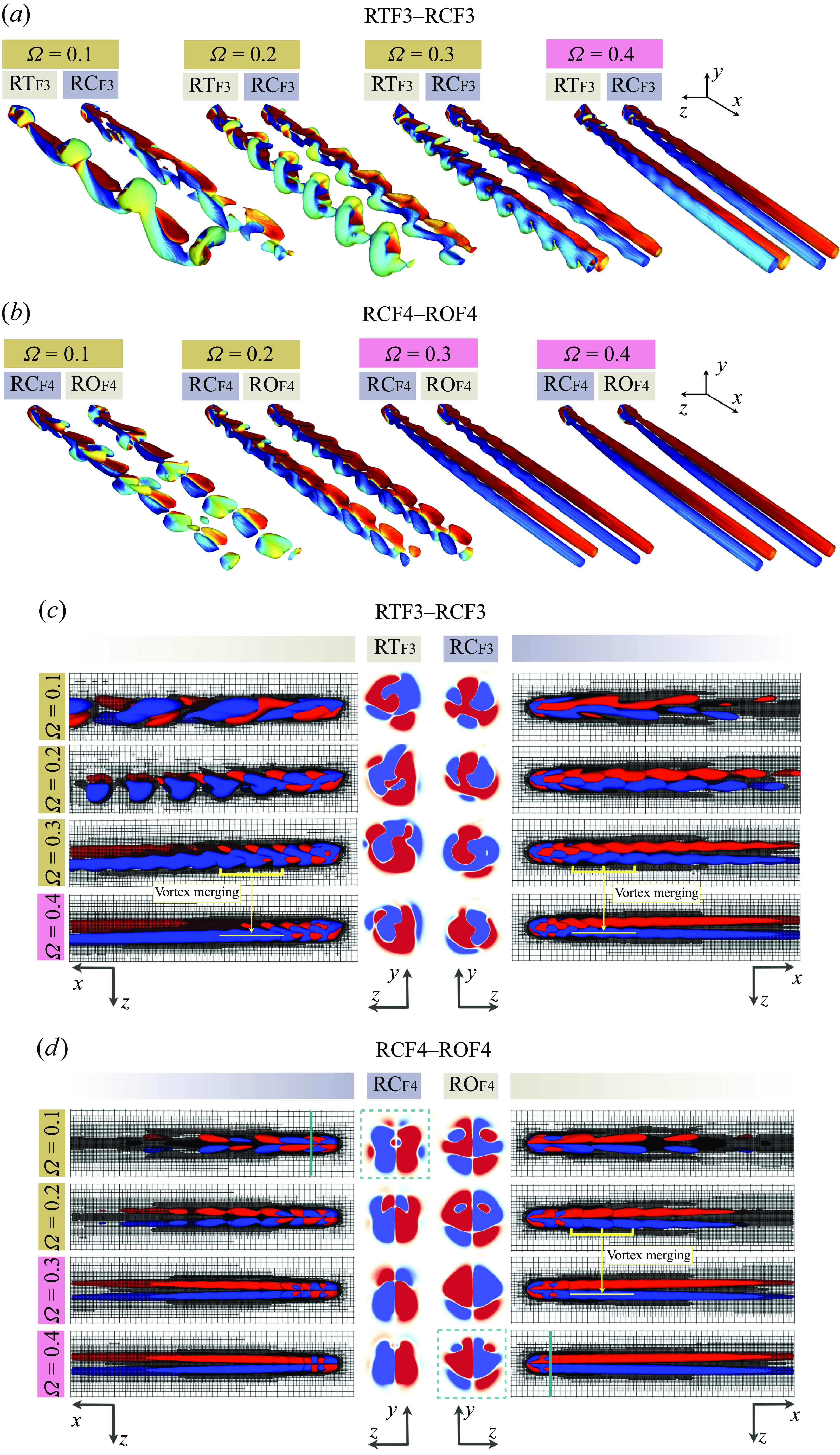
Figure 17. Evolution of wake structures before and after the vortex suppression in the flow past a rotating angular particle at ${{R}e}=100$
. Side view of the wake structures, identified by
${{R}e}=100$
. Side view of the wake structures, identified by $\lambda _2=-1$
and coloured by
$\lambda _2=-1$
and coloured by $u_x$
, are shown for comparison between the (a) three-fold cases and (b) four-fold cases. Top views of the wake structures, identified by vorticity
$u_x$
, are shown for comparison between the (a) three-fold cases and (b) four-fold cases. Top views of the wake structures, identified by vorticity $\omega _x=\pm 0.03$
in the
$\omega _x=\pm 0.03$
in the $x$
-
$x$
- $z$
plane, are compared for the (c) three-fold cases and (d) four-fold cases. The
$z$
plane, are compared for the (c) three-fold cases and (d) four-fold cases. The $\omega _x$
distribution in the
$\omega _x$
distribution in the $y$
-
$y$
- $z$
plane at
$z$
plane at $x=x_p+1.5$
are also depicted in panels (c) and (d).
$x=x_p+1.5$
are also depicted in panels (c) and (d).
5.2. Impact of particle angularity on hydrodynamic forces
We now shift our attention from the wake structure to the rotating particle itself, examining how $\phi$
and
$\phi$
and $n_{\Omega }$
affect the hydrodynamic forces acting on the particle. Figure 18 illustrates the evolution of
$n_{\Omega }$
affect the hydrodynamic forces acting on the particle. Figure 18 illustrates the evolution of $\overline {C_{l,y}}$
of the three angular particles – RTF3, RCF3 and ROF4 – as a function of increasing
$\overline {C_{l,y}}$
of the three angular particles – RTF3, RCF3 and ROF4 – as a function of increasing $\Omega$
at
$\Omega$
at ${{R}e} = 60$
–
${{R}e} = 60$
– $160$
. It is clear that
$160$
. It is clear that $\overline {C_{l,y}}$
increases monotonically with
$\overline {C_{l,y}}$
increases monotonically with $\Omega$
at any given
$\Omega$
at any given ${R}e$
. At
${R}e$
. At ${{R}e} = 60$
, particle angularity has a pronounced effect, significantly amplifying the lift. The rotating tetrahedron RTF3 in figure 18(a) reaches
${{R}e} = 60$
, particle angularity has a pronounced effect, significantly amplifying the lift. The rotating tetrahedron RTF3 in figure 18(a) reaches $\overline {C_{l,y}} = 1.12$
, which is 15 % higher than RCF3 in figure 18(b) and 20 % higher than ROF4 in figure 18(c). As flow inertia increases,
$\overline {C_{l,y}} = 1.12$
, which is 15 % higher than RCF3 in figure 18(b) and 20 % higher than ROF4 in figure 18(c). As flow inertia increases, $\overline {C_{l,y}}$
tends to decrease. By
$\overline {C_{l,y}}$
tends to decrease. By ${{R}e} = 160$
, the influence of particle angularity diminishes, especially at higher rotation rates. For instance, at
${{R}e} = 160$
, the influence of particle angularity diminishes, especially at higher rotation rates. For instance, at $\Omega = 1$
, all three angular particles exhibit the same lift coefficient
$\Omega = 1$
, all three angular particles exhibit the same lift coefficient $\overline {C_{l,y}} = 0.75$
.
$\overline {C_{l,y}} = 0.75$
.
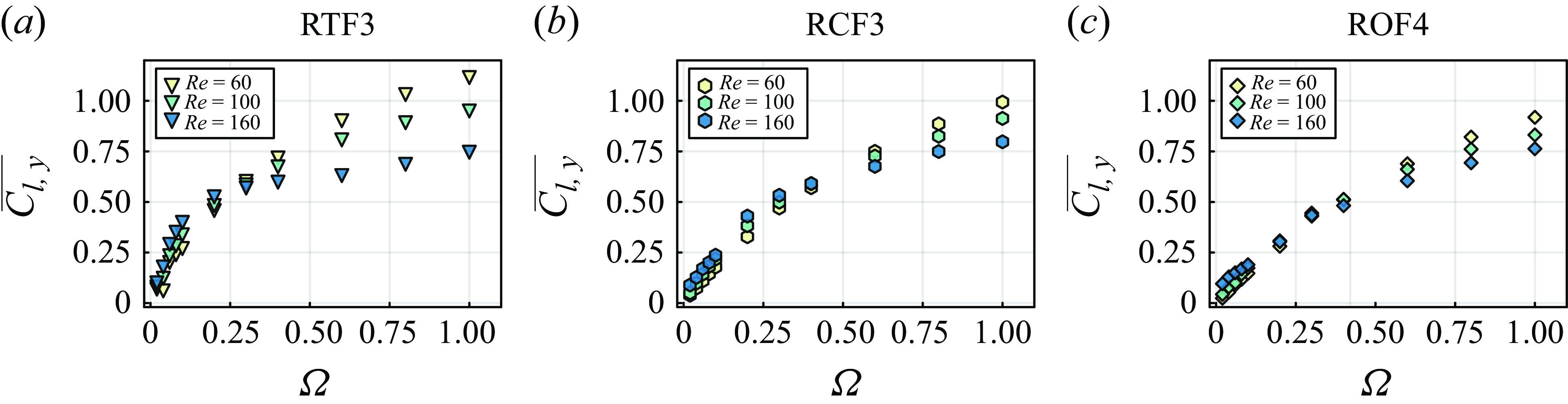
Figure 18. Evolution of $\overline {C_{l,y}}$
of a rotating angular particle as a function of
$\overline {C_{l,y}}$
of a rotating angular particle as a function of $\Omega$
at
$\Omega$
at ${{R}e} = 60$
,
${{R}e} = 60$
, $100$
and
$100$
and $160$
: (a) RTF3; (b) RCF3 and (c) ROF4.
$160$
: (a) RTF3; (b) RCF3 and (c) ROF4.
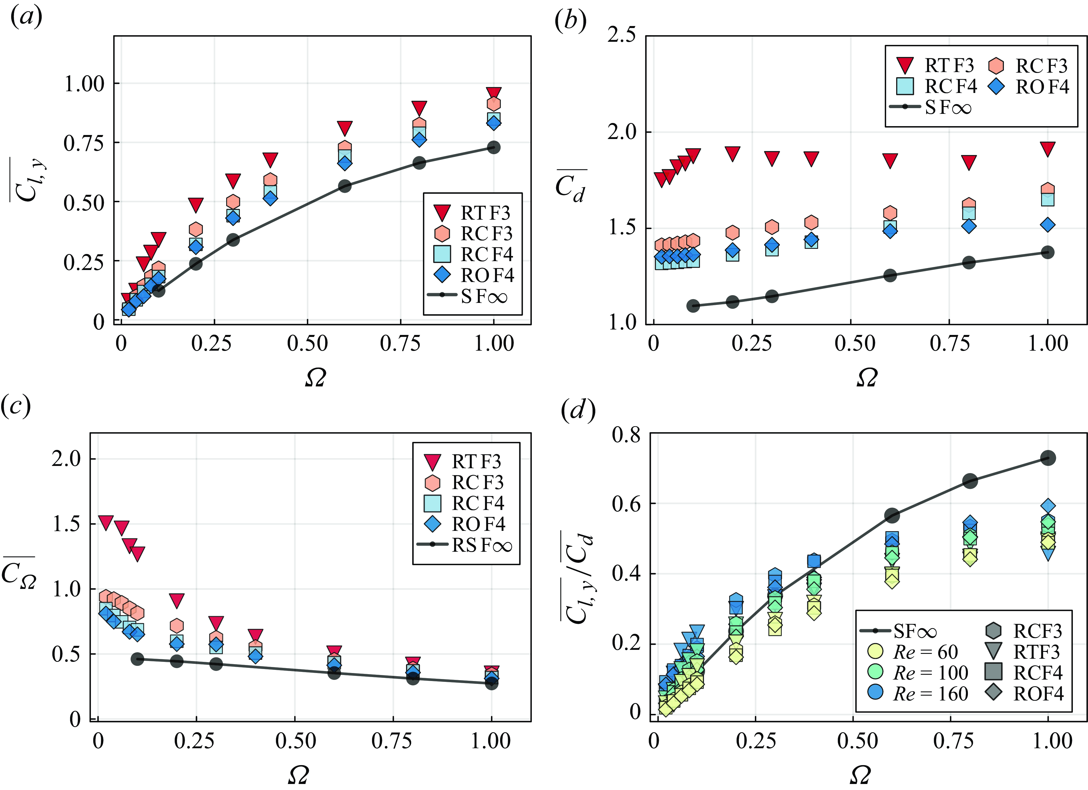
Figure 19. Effects of particle angularity on the hydrodynamic forces exerted on a rotating angular particle: (a) lift coefficient $\overline {C_{l,y}}$
at
$\overline {C_{l,y}}$
at ${{R}e}=100$
; (b) drag coefficient
${{R}e}=100$
; (b) drag coefficient $\overline {C_{d}}$
at
$\overline {C_{d}}$
at ${{R}e}=100$
; (c) rotation coefficient
${{R}e}=100$
; (c) rotation coefficient $\overline {C_{\Omega }}$
at
$\overline {C_{\Omega }}$
at ${{R}e}=100$
and (d) the lift-to-drag ratio
${{R}e}=100$
and (d) the lift-to-drag ratio $\overline {C_{l,y}}/\overline {C_{d}}$
at
$\overline {C_{l,y}}/\overline {C_{d}}$
at ${{R}e}=60$
–
${{R}e}=60$
– $160$
. The case of the flow past a rotating
$160$
. The case of the flow past a rotating $RSF\infty$
sphere at
$RSF\infty$
sphere at ${{R}e}=100$
is provided as a reference and shown by the black solid lines.
${{R}e}=100$
is provided as a reference and shown by the black solid lines.
Recognising that particle shape has a more pronounced impact in low-inertia flows, we fix ${{R}e} = 100$
and examine the evolution of the lift, drag and rotation coefficients in figure 19 to gain deeper insights into the hydrodynamic behaviour. Figure 19(a) illustrates the evolution of
${{R}e} = 100$
and examine the evolution of the lift, drag and rotation coefficients in figure 19 to gain deeper insights into the hydrodynamic behaviour. Figure 19(a) illustrates the evolution of $\overline {C_{l,y}}$
as a function of
$\overline {C_{l,y}}$
as a function of $\Omega$
for all the shapes examined in this study. It is clear that particle angularity enhances the Magnus effect, leading to higher
$\Omega$
for all the shapes examined in this study. It is clear that particle angularity enhances the Magnus effect, leading to higher $\overline {C_{l,y}}$
. Particles with a three-fold symmetry axis generate higher lift compared with those with a four-fold symmetry axis, and both significantly outperform the sphere, which represents the infinite-fold symmetry case (RSF
$\overline {C_{l,y}}$
. Particles with a three-fold symmetry axis generate higher lift compared with those with a four-fold symmetry axis, and both significantly outperform the sphere, which represents the infinite-fold symmetry case (RSF $\infty$
). Additionally,
$\infty$
). Additionally, $\overline {C_d}$
is affected by
$\overline {C_d}$
is affected by $\phi$
, with the tetrahedron showing significantly higher values than the other shapes, as seen in figure 19(b). This behaviour results from the large recirculation region volume
$\phi$
, with the tetrahedron showing significantly higher values than the other shapes, as seen in figure 19(b). This behaviour results from the large recirculation region volume $V_r$
in the RTF3 case, as depicted in figure 24(e) in Appendix D. Here,
$V_r$
in the RTF3 case, as depicted in figure 24(e) in Appendix D. Here, $\overline {C_d}$
of RTF3 increases until
$\overline {C_d}$
of RTF3 increases until $\Omega = 0.1$
, after which it stabilises around
$\Omega = 0.1$
, after which it stabilises around $1.9$
and remains constant up to
$1.9$
and remains constant up to $\Omega = 1$
. Meanwhile, RCF3 exhibits slightly higher drag values than RCF4 and ROF4. All angular particles exhibit higher
$\Omega = 1$
. Meanwhile, RCF3 exhibits slightly higher drag values than RCF4 and ROF4. All angular particles exhibit higher $\overline {C_d}$
than the rotating sphere.
$\overline {C_d}$
than the rotating sphere.
The $\overline {C_{\Omega }}$
increases when particle angularity increases, as shown in figure 19(c), demonstrating that sharp edges enhance the efficiency of the Magnus effect. It is especially pronounced in slow-rotating cases
$\overline {C_{\Omega }}$
increases when particle angularity increases, as shown in figure 19(c), demonstrating that sharp edges enhance the efficiency of the Magnus effect. It is especially pronounced in slow-rotating cases $\Omega \leqslant 0.6$
. For example, at
$\Omega \leqslant 0.6$
. For example, at $\Omega = 0.1$
, RTF3 exhibits a
$\Omega = 0.1$
, RTF3 exhibits a $\overline {C_{\Omega }}$
two and a half times greater than that of the sphere. However, as the rotation rate increases, the influence of particle angularity diminishes and
$\overline {C_{\Omega }}$
two and a half times greater than that of the sphere. However, as the rotation rate increases, the influence of particle angularity diminishes and $\overline {C_{\Omega }}$
in all cases converges to a similar value of
$\overline {C_{\Omega }}$
in all cases converges to a similar value of $0.35$
at
$0.35$
at $\Omega = 1$
, where particle shape no longer plays a significant role. Figure 19(d) illustrates the evolution of the ratio
$\Omega = 1$
, where particle shape no longer plays a significant role. Figure 19(d) illustrates the evolution of the ratio $\overline {C_{l,y}}/\overline {C_{d}}$
for particles of various shapes at
$\overline {C_{l,y}}/\overline {C_{d}}$
for particles of various shapes at ${{R}e} = 60$
–
${{R}e} = 60$
– $160$
. Unlike the individual lift and drag coefficients,
$160$
. Unlike the individual lift and drag coefficients, $\overline {C_{l,y}}/\overline {C_{d}}$
shows very limited dependence on particle angularity. In contrast, flow inertia plays a more noticeable role, contributing to the increase of the ratio. It is noteworthy that the rotating sphere (plotted in black solid line for
$\overline {C_{l,y}}/\overline {C_{d}}$
shows very limited dependence on particle angularity. In contrast, flow inertia plays a more noticeable role, contributing to the increase of the ratio. It is noteworthy that the rotating sphere (plotted in black solid line for ${{R}e} = 100$
) exhibits values comparable to the angular particles at
${{R}e} = 100$
) exhibits values comparable to the angular particles at $\Omega \leqslant 0.4$
. However, at
$\Omega \leqslant 0.4$
. However, at $\Omega \geqslant 0.6$
, the sphere shows higher values than the angular particles, as indicated by the light green markers. Remarkably, for all particle shapes, the ratio
$\Omega \geqslant 0.6$
, the sphere shows higher values than the angular particles, as indicated by the light green markers. Remarkably, for all particle shapes, the ratio $\overline {C_{l,y}}/\overline {C_{d}}$
remains consistently bounded by
$\overline {C_{l,y}}/\overline {C_{d}}$
remains consistently bounded by $0.6$
across the entire range of
$0.6$
across the entire range of $0.02 \leqslant \Omega \leqslant 1$
. The upper bound
$0.02 \leqslant \Omega \leqslant 1$
. The upper bound $0.6$
also holds true for all
$0.6$
also holds true for all $40 \leqslant {{R}e} \leqslant 400$
considered in RCF4 cases, as shown in figure 12(b). This key finding reveals a consistent upper limit on the lift-to-drag ratio of flow past a rotating angular particle, independent of particle shape and rotation rate. In addition to affecting hydrodynamic forces, increased particle angularity substantially amplifies hydrodynamic torques. Further details on how particle angularity influences
$40 \leqslant {{R}e} \leqslant 400$
considered in RCF4 cases, as shown in figure 12(b). This key finding reveals a consistent upper limit on the lift-to-drag ratio of flow past a rotating angular particle, independent of particle shape and rotation rate. In addition to affecting hydrodynamic forces, increased particle angularity substantially amplifies hydrodynamic torques. Further details on how particle angularity influences $\overline {T_z}$
are provided in Appendix F.
$\overline {T_z}$
are provided in Appendix F.
5.3. Role of effective faces in determining shedding frequency
From the previous sections, we know that $n_{\Omega }$
significantly influences vortex generation, while
$n_{\Omega }$
significantly influences vortex generation, while $\phi$
has a greater impact on the hydrodynamic forces. We now shift our focus to the shedding frequency, a crucial aspect of wake dynamics driven by vortex shedding. The key question we aim to address is how
$\phi$
has a greater impact on the hydrodynamic forces. We now shift our focus to the shedding frequency, a crucial aspect of wake dynamics driven by vortex shedding. The key question we aim to address is how $n_{\Omega }$
of different angular particles affects
$n_{\Omega }$
of different angular particles affects $\mathcal{S}\textit{tr}$
. Similarly to what we did to produce figure 14, we apply FFT to the temporal evolution of
$\mathcal{S}\textit{tr}$
. Similarly to what we did to produce figure 14, we apply FFT to the temporal evolution of $C_{l,y}$
for RTF3, ROF4 and RCF3, and compute the corresponding
$C_{l,y}$
for RTF3, ROF4 and RCF3, and compute the corresponding $\mathcal{S}\textit{tr}$
values, shown in figure 20.
$\mathcal{S}\textit{tr}$
values, shown in figure 20.
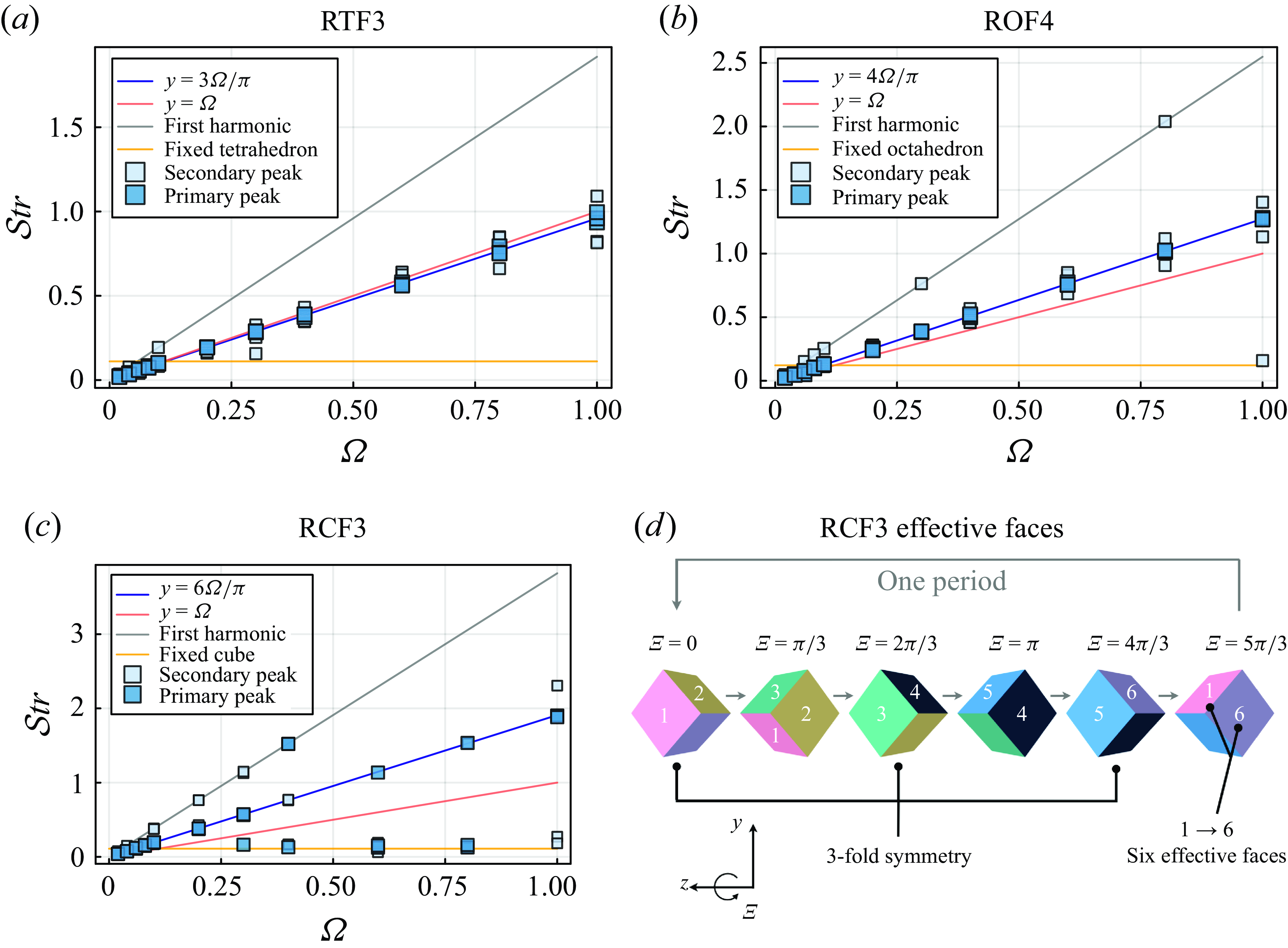
Figure 20. $\mathcal{S}\textit{tr}$
of the primary and secondary peaks as a function of
$\mathcal{S}\textit{tr}$
of the primary and secondary peaks as a function of $\Omega$
for (a) RTF3, (b) ROF4 and (c) RCF3. The blue curve represents the proposed model for the primary peak
$\Omega$
for (a) RTF3, (b) ROF4 and (c) RCF3. The blue curve represents the proposed model for the primary peak $\mathcal{S}\textit{tr}_1$
, while the red curve corresponds to
$\mathcal{S}\textit{tr}_1$
, while the red curve corresponds to $y = \Omega$
. The grey curve indicates the first harmonic of the primary peak frequency, and the yellow curve denotes the characteristic
$y = \Omega$
. The grey curve indicates the first harmonic of the primary peak frequency, and the yellow curve denotes the characteristic $\mathcal{S}\textit{tr}_0$
of the flow past a fixed tetrahedron
$\mathcal{S}\textit{tr}_0$
of the flow past a fixed tetrahedron $\mathcal{S}\textit{tr}_0=0.11$
in panel (a), a fixed octahedron
$\mathcal{S}\textit{tr}_0=0.11$
in panel (a), a fixed octahedron $\mathcal{S}\textit{tr}_0=0.12$
in panel (b) and a fixed cube
$\mathcal{S}\textit{tr}_0=0.12$
in panel (b) and a fixed cube $\mathcal{S}\textit{tr}_0=0.11$
in panel (c) (Gai & Wachs Reference Gai and Wachs2023b
). (d) Rear view of RCF3 with snapshots showing incremental rotation angles (
$\mathcal{S}\textit{tr}_0=0.11$
in panel (c) (Gai & Wachs Reference Gai and Wachs2023b
). (d) Rear view of RCF3 with snapshots showing incremental rotation angles ( $\varDelta \Xi = \pi /3$
) over a complete rotation period, where the six effective faces of RCF3 are depicted in different colours.
$\varDelta \Xi = \pi /3$
) over a complete rotation period, where the six effective faces of RCF3 are depicted in different colours.
As discussed in the RCF4 case, each effective face generates a pair of oppositely signed upper/lower streamwise vortices as it pushes fluid into the wake. Since RCF4 has four effective faces, it produces four pairs of upper/lower streamwise vortices per rotation period. Extending this mechanism to other angular particles, we hypothesise that the number of vortex pairs generated per period is proportional to the number of effective faces $N_{\mathcal{F}}$
. In Fourier space, this implies that
$N_{\mathcal{F}}$
. In Fourier space, this implies that $\mathcal{S}\textit{tr}$
associated with the primary peak should be proportional to
$\mathcal{S}\textit{tr}$
associated with the primary peak should be proportional to $N_{\mathcal{F}}$
. Based on this reasoning, we propose the following model for
$N_{\mathcal{F}}$
. Based on this reasoning, we propose the following model for $\mathcal{S}\textit{tr}_1$
, as derived from (4.2):
$\mathcal{S}\textit{tr}_1$
, as derived from (4.2):
 \begin{equation} \mathcal{S}\textit{tr}_1 = \frac {N_{\mathcal{F}}}{\pi }\Omega . \end{equation}
We plot the prediction of $\mathcal{S}\textit{tr}_1$
from (5.1) for the RTF3 case as a function of
$\mathcal{S}\textit{tr}_1$
from (5.1) for the RTF3 case as a function of $\Omega$
and compare it with the numerical results in figure 20(a). RTF3 has a three-fold rotational symmetry, corresponding to three effective faces
$\Omega$
and compare it with the numerical results in figure 20(a). RTF3 has a three-fold rotational symmetry, corresponding to three effective faces $N_{\mathcal{F}} = 3$
. As shown in figure 20(a), the numerical data align closely with the prediction from (5.1), with all primary peaks falling along the prediction curve (navy solid line). The secondary peaks also follow the primary peaks closely. Similarly, in the ROF4 case (figure 20
b), the primary peaks match very well the model prediction, with
$N_{\mathcal{F}} = 3$
. As shown in figure 20(a), the numerical data align closely with the prediction from (5.1), with all primary peaks falling along the prediction curve (navy solid line). The secondary peaks also follow the primary peaks closely. Similarly, in the ROF4 case (figure 20
b), the primary peaks match very well the model prediction, with $N_{\mathcal{F}} = 4$
. Several secondary peaks appear along the first harmonic curve, indicating intensified vortex interactions.
$N_{\mathcal{F}} = 4$
. Several secondary peaks appear along the first harmonic curve, indicating intensified vortex interactions.
RCF3 presents a unique case because, although it has a three-fold rotational symmetry, each fold consists of two effective faces, resulting in a total of six effective faces, compared with only three in the RTF3 case. In figure 20(d), we show a rear view of RCF3 with snapshots illustrating incremental rotation angles $\varDelta \Xi = \pi /3$
over a complete rotation period around the
$\varDelta \Xi = \pi /3$
over a complete rotation period around the $z$
-axis. Starting from the initial angular position at
$z$
-axis. Starting from the initial angular position at $\Xi = 0$
, each rotation by
$\Xi = 0$
, each rotation by $\varDelta \Xi = 2\pi /3$
returns the cube to the same angular position, confirming its three-fold rotational symmetry. In figure 20(d), the six distinct faces, each highlighted in a different colour, all contribute to pushing fluid into the wake region during a single period, leading to
$\varDelta \Xi = 2\pi /3$
returns the cube to the same angular position, confirming its three-fold rotational symmetry. In figure 20(d), the six distinct faces, each highlighted in a different colour, all contribute to pushing fluid into the wake region during a single period, leading to $N_{\mathcal{F}} = 6$
. As a result, the frequency distribution in figure 20(c) shows distinct behaviour compared with figure 20(a). While most of the primary peaks align well with the prediction of (5.1), several primary peaks correspond to
$N_{\mathcal{F}} = 6$
. As a result, the frequency distribution in figure 20(c) shows distinct behaviour compared with figure 20(a). While most of the primary peaks align well with the prediction of (5.1), several primary peaks correspond to $\mathcal{S}\textit{tr}_0$
, i.e. to the Strouhal number of the flow past a fixed cube. This occurs because, at higher shedding frequencies (with six pairs of vortices per period), the streamwise upper vortex pairs generated by each effective face become relatively weak, allowing the build-up and release process of the recirculation region in the lower wake to dominate. Additionally, more secondary peaks appear along the first harmonic curve.
$\mathcal{S}\textit{tr}_0$
, i.e. to the Strouhal number of the flow past a fixed cube. This occurs because, at higher shedding frequencies (with six pairs of vortices per period), the streamwise upper vortex pairs generated by each effective face become relatively weak, allowing the build-up and release process of the recirculation region in the lower wake to dominate. Additionally, more secondary peaks appear along the first harmonic curve.
Although $N_{\mathcal{F}}$
directly influences
$N_{\mathcal{F}}$
directly influences $\mathcal{S}\textit{tr}_1$
, the vortex suppression is noted to be primarily governed by
$\mathcal{S}\textit{tr}_1$
, the vortex suppression is noted to be primarily governed by $n_{\Omega }$
. Recall that in cases of low flow inertia, vortex suppression occurs at
$n_{\Omega }$
. Recall that in cases of low flow inertia, vortex suppression occurs at $\Omega = 0.3$
for RCF4 and ROF4, and at
$\Omega = 0.3$
for RCF4 and ROF4, and at $\Omega = 0.4$
for RTF3 and RCF3. An intriguing observation is that multiplying these critical rotation rates by the corresponding number of rotational symmetry folds yields a critical Strouhal number,
$\Omega = 0.4$
for RTF3 and RCF3. An intriguing observation is that multiplying these critical rotation rates by the corresponding number of rotational symmetry folds yields a critical Strouhal number, $\mathcal{S}\textit{tr}_c = n_{\Omega }\Omega _c/\pi \approx 0.38$
, which is nearly four times the characteristic Strouhal number of the flow past a fixed angular particle,
$\mathcal{S}\textit{tr}_c = n_{\Omega }\Omega _c/\pi \approx 0.38$
, which is nearly four times the characteristic Strouhal number of the flow past a fixed angular particle, $\mathcal{S}\textit{tr}_0 \approx 0.1$
. This suggests that the shedding frequency of streamwise vortex pairs driven by the effective faces must be sufficiently high to promote vortex merging, eventually leading to suppression. For angular particles, this process can be more easily controlled, as the finite number of effective faces allows for fine-tuning of the shedding frequency to stabilise the wake.
$\mathcal{S}\textit{tr}_0 \approx 0.1$
. This suggests that the shedding frequency of streamwise vortex pairs driven by the effective faces must be sufficiently high to promote vortex merging, eventually leading to suppression. For angular particles, this process can be more easily controlled, as the finite number of effective faces allows for fine-tuning of the shedding frequency to stabilise the wake.
6. Conclusions
We explored the dynamics, wake instabilities and regime transitions of inertial flow past transversely rotating angular particles. Our findings provide new insights into how particle angularity and rotational symmetry fold influence flow instabilities, deepening our understanding of how sharp edges affect inertial flow.
By investigating the rotating cube (RCF4, four-fold cube), we find the driving mechanisms of vortex generation on the front inclined faces, and the merging process on the cube surface and in the wake region. Our results reveal intricate vortex shedding structures, and show that the generation and merging of streamwise vortex pairs are key mechanisms leading to vortex suppression. The four effective faces of RCF4 produce four pairs of opposite-signed upper/lower streamwise vortices per rotation period. At low rotation rates, $\Omega \leqslant 0.2$
, rotation induces periodic impulses to the wake, resulting in periodic hairpin vortex shedding at lower
$\Omega \leqslant 0.2$
, rotation induces periodic impulses to the wake, resulting in periodic hairpin vortex shedding at lower ${R}e$
compared with a fixed cube. However, as the rotation rate increases to
${R}e$
compared with a fixed cube. However, as the rotation rate increases to $\Omega = 0.3$
, the higher shedding frequency of streamwise vortex pairs promotes the merging of vortices with the same sign, leading to vortex suppression and wake stabilisation. At even higher rotation rates, the stabilised wake becomes wavy further downstream due to the onset of Kelvin–Helmholtz instabilities, similar to the rotating sphere.
$\Omega = 0.3$
, the higher shedding frequency of streamwise vortex pairs promotes the merging of vortices with the same sign, leading to vortex suppression and wake stabilisation. At even higher rotation rates, the stabilised wake becomes wavy further downstream due to the onset of Kelvin–Helmholtz instabilities, similar to the rotating sphere.
A detailed analysis of the hydrodynamic forces, with a focus on the Magnus effect, reveals how the sharp edges of the particle significantly influence the lift, drag, rotation coefficients and the shedding frequency. In low-inertia flows, ${{R}e} \leqslant 200$
, an intriguing fixed point is observed in the evolution of
${{R}e} \leqslant 200$
, an intriguing fixed point is observed in the evolution of $\overline {C_{l,y}}$
. At
$\overline {C_{l,y}}$
. At $\Omega = 0.4$
, the Magnus effect becomes largely independent of flow inertia, with
$\Omega = 0.4$
, the Magnus effect becomes largely independent of flow inertia, with $\overline {C_{l,y}}$
stabilising at a constant value of
$\overline {C_{l,y}}$
stabilising at a constant value of $0.5$
, regardless of
$0.5$
, regardless of ${R}e$
. The evolution of drag and rotation coefficients also exhibits unique behaviours due to the sharp edges of the cube. The spectrum of shedding frequency of RCF4 shows that the primary peak in the frequency spectrum is directly linked to the shedding of streamwise vortex pairs.
${R}e$
. The evolution of drag and rotation coefficients also exhibits unique behaviours due to the sharp edges of the cube. The spectrum of shedding frequency of RCF4 shows that the primary peak in the frequency spectrum is directly linked to the shedding of streamwise vortex pairs.
We then extend the analysis to general angular particles with different numbers of rotational symmetry folds $n_{\Omega }$
: RTF3 (three-fold tetrahedron), RCF3 (three-fold cube) and ROF4 (four-fold octahedron). We demonstrate that particle shape and rotation have a significant impact on wake stability, regime transitions and the resulting hydrodynamic forces. The vortex generation and suppression mechanisms observed for RCF4 are found to hold for other angular particles, with
$n_{\Omega }$
: RTF3 (three-fold tetrahedron), RCF3 (three-fold cube) and ROF4 (four-fold octahedron). We demonstrate that particle shape and rotation have a significant impact on wake stability, regime transitions and the resulting hydrodynamic forces. The vortex generation and suppression mechanisms observed for RCF4 are found to hold for other angular particles, with $n_{\Omega }$
emerging as a key factor in determining regime transitions. Additionally, the number of effective faces
$n_{\Omega }$
emerging as a key factor in determining regime transitions. Additionally, the number of effective faces $N_{\mathcal{F}}$
alters the topology of the wake structures. In contrast, particle angularity
$N_{\mathcal{F}}$
alters the topology of the wake structures. In contrast, particle angularity $\phi$
plays a more dominant role in hydrodynamic forces, with higher angularity enhancing the Magnus effect especially in the low inertia flow. Using
$\phi$
plays a more dominant role in hydrodynamic forces, with higher angularity enhancing the Magnus effect especially in the low inertia flow. Using $N_{\mathcal{F}}$
, we propose a generic model to predict the Strouhal number, which accurately captures the primary peaks of the frequency spectrum
$N_{\mathcal{F}}$
, we propose a generic model to predict the Strouhal number, which accurately captures the primary peaks of the frequency spectrum $\mathcal{S}\textit{tr}_1$
. We further show that increased
$\mathcal{S}\textit{tr}_1$
. We further show that increased $n_{\Omega }$
promotes vortex merging and suppression. Ultimately, this study demonstrates that wake flow stability can be effectively harnessed through the interplay between particle shape (
$n_{\Omega }$
promotes vortex merging and suppression. Ultimately, this study demonstrates that wake flow stability can be effectively harnessed through the interplay between particle shape ( $\phi$
,
$\phi$
, $N_{\mathcal{F}}$
) and rotational properties (
$N_{\mathcal{F}}$
) and rotational properties ( $\Omega$
,
$\Omega$
, $n_{\Omega }$
).
$n_{\Omega }$
).
This study presents a decoupled perspective on the complex interactions between a rotating particle and the surrounding fluid under controlled conditions. While freely moving particles introduce additional complexities– such as varying angular positions, added mass effects and particle–particle interactions– the findings from centre-fixed rotating particles provide valuable insights to comprehensively understand force balance and wake structure evolutions. These insights, in turn, aid in predicting the trajectories and regime transitions of freely settling angular particles. In addition, the deeper understanding we offer paves the way for advancements in controlling flow instabilities and optimising system designs across a variety of applications. Future research could explore a broader parameter space, particularly at $\Omega \geqslant 1$
, to determine the threshold at which the influence of particle angularity becomes negligible and the effects of rotation dominate. This would provide a clearer understanding of when angularity can be disregarded in favour of rotational effects in flow stabilisation. Another intriguing direction would be to investigate streamwise rotating angular particles and compare their wake dynamics with those of the transversely rotating angular particles studied in this paper. Such a study could provide valuable perspectives into the most effective rotational strategies for stabilising the wake flow past angular particles.
$\Omega \geqslant 1$
, to determine the threshold at which the influence of particle angularity becomes negligible and the effects of rotation dominate. This would provide a clearer understanding of when angularity can be disregarded in favour of rotational effects in flow stabilisation. Another intriguing direction would be to investigate streamwise rotating angular particles and compare their wake dynamics with those of the transversely rotating angular particles studied in this paper. Such a study could provide valuable perspectives into the most effective rotational strategies for stabilising the wake flow past angular particles.
Acknowledgement
Guodong Gai expresses his gratitude to the Pacific Institute of Mathematical Sciences for their support via his PIMS-CNRS postdoctoral fellowship.
Funding
The authors greatly appreciate the financial support of the Natural Sciences and Engineering Research Council of Canada (NSERC) via Anthony Wachs New Frontiers in Research Fund grant NFRFE-2018–01922. This research was enabled by support provided by Digital Research Alliance of Canada (https://alliancecan.ca/en) through Anthony Wachs’ 2023–2024 Computing Resources for Research Groups allocation qpf-764-ac. This research was also supported in part through computational resources and services provided by Advanced Research Computing at the University of British Columbia (https://arc.ubc.ca).
Declaration of interests
The authors report no conflict of interest.
Appendix A. Distributed Lagrange multiplier/fictitious domain (DLM/FD) method
The governing equations for conservation of mass and momentum in an incompressible Newtonian fluid are given by
 \begin{align}& \rho _f^*\left (\frac {\partial \boldsymbol{u}^*}{\partial t^*} + \boldsymbol{u}^*\cdot \nabla \boldsymbol{u}^*\right ) = -\nabla p^* + \mu _f^* \Delta {\boldsymbol{u}}^* \,\,\,\, \mbox{in} \ \mathcal{D}\setminus P, \end{align}
 \begin{align}&\qquad\qquad\qquad\,\,\, \nabla \cdot \boldsymbol{u}^*=0 \,\,\,\, \mbox{in} \ \mathcal{D}\setminus P, \\[6pt] \nonumber \end{align}
where $\boldsymbol{u}^*$
denotes the fluid velocity vector,
$\boldsymbol{u}^*$
denotes the fluid velocity vector, $p^*$
represents the pressure,
$p^*$
represents the pressure, $\mathcal{D}$
is the computational domain and
$\mathcal{D}$
is the computational domain and $P$
refers to the solid particle.
$P$
refers to the solid particle.
The particle rotates around the z-axis with an imposed constant angular velocity, $\boldsymbol{\Omega ^*}$
, which remains unchanged throughout the simulations. The hydrodynamic force and torque (relative to the centre of mass) acting on the particle
$\boldsymbol{\Omega ^*}$
, which remains unchanged throughout the simulations. The hydrodynamic force and torque (relative to the centre of mass) acting on the particle $\boldsymbol{F^*}$
and
$\boldsymbol{F^*}$
and $\boldsymbol{T^*}$
are
$\boldsymbol{T^*}$
are
 \begin{align}&\quad\,\,\, \boldsymbol{F^*} = \int _{\partial P} \boldsymbol{\sigma ^*}\cdot \boldsymbol{\hat {n}}\,{\rm d}S^*, \end{align}
 \begin{align}& \boldsymbol{T^*} = \int _{\partial P} \boldsymbol{r^*}\times \left (\boldsymbol{\sigma ^*}\cdot \boldsymbol{\hat {n}}\right )\,{\rm d}S^*, \end{align}
where $\boldsymbol{\hat {n}}$
is the outward-pointing unit normal vector to the particle surface
$\boldsymbol{\hat {n}}$
is the outward-pointing unit normal vector to the particle surface $\partial P$
, and the stress tensor for a Newtonian fluid is given by:
$\partial P$
, and the stress tensor for a Newtonian fluid is given by:
 \begin{equation} \boldsymbol{\sigma ^*} = -p^*\boldsymbol{I_d} + 2\mu _f^*\boldsymbol{D[u]^*}. \end{equation}
The DLM/FD method combines the weak formulations of the fluid motion equation and the rigid particle motion equation to derive the governing equation for the fluid–particle mixture. First, the weak formulation for the fluid sub-domain $\mathcal{D} \setminus P$
is derived by enforcing rigid-body constraints on the particle surface
$\mathcal{D} \setminus P$
is derived by enforcing rigid-body constraints on the particle surface $\partial P$
. This formulation is then extended to the entire computational domain
$\partial P$
. This formulation is then extended to the entire computational domain $\mathcal{D}$
by applying the rigid-body constraints across the entire particle domain
$\mathcal{D}$
by applying the rigid-body constraints across the entire particle domain $P$
, leading to the combined equation of motion. The rigid-body motion constraints within the particle sub-domain are relaxed through the use of Lagrange multipliers, denoted as
$P$
, leading to the combined equation of motion. The rigid-body motion constraints within the particle sub-domain are relaxed through the use of Lagrange multipliers, denoted as $\boldsymbol{\lambda }^*$
. We define
$\boldsymbol{\lambda }^*$
. We define $\mathcal{W}_\Gamma$
,
$\mathcal{W}_\Gamma$
, $\mathcal{W}_0$
,
$\mathcal{W}_0$
, $\mathcal{L}_0$
and
$\mathcal{L}_0$
and $\Lambda$
as the functional spaces of the solution that satisfy the boundary conditions (Selçuk et al. Reference Selçuk, Ghigo, Popinet and Wachs2021).
$\Lambda$
as the functional spaces of the solution that satisfy the boundary conditions (Selçuk et al. Reference Selçuk, Ghigo, Popinet and Wachs2021).
Next, we consider the following constrained optimisation problem for a single rotating particle $P$
: find
$P$
: find $\boldsymbol{u^*} \in \mathcal{W}_\Gamma$
,
$\boldsymbol{u^*} \in \mathcal{W}_\Gamma$
, $p^*\in \mathcal{L}^2_0$
and
$p^*\in \mathcal{L}^2_0$
and $\boldsymbol{\lambda }^*\in \Lambda$
such that we obtain the following.
$\boldsymbol{\lambda }^*\in \Lambda$
such that we obtain the following.
-
(i) Combined equations of motion:
(A6)
\begin{align} &\int _{\mathcal{D}} \rho _f^* \left (\frac {\partial \boldsymbol{u}^*}{\partial t^*} + \boldsymbol{u}^*\cdot \nabla \boldsymbol{u}^*\right )\cdot \boldsymbol{v}^*\,{\rm d}\boldsymbol{x} - \int _{\mathcal{D}}p^*\nabla \cdot \boldsymbol{v}^*{\rm d}\boldsymbol{x} \end{align}
(A7)
\begin{align} &\qquad + \int _{\mathcal{D}}\mu _f^*\nabla \boldsymbol{u}^*:\nabla \boldsymbol{v}^*{\rm d}\boldsymbol{x} = -\int _{P}\boldsymbol{\lambda }^*\cdot \boldsymbol{v}^*\,{\rm d}\boldsymbol{x}. \end{align}
-
(ii) Continuity equation:
(A8)
\begin{equation} \int _{\mathcal{D}} -q^*\nabla \cdot \boldsymbol{u}^*\,{\rm d}\boldsymbol{x} = 0. \end{equation}
-
(iii) For the particle:
(A9)
\begin{align}& \left (1-\frac {\rho _f^*}{\rho _p^*}\right )\frac {{\rm d}\boldsymbol{I^*\Omega ^*}}{{\rm d}t^*}\cdot \boldsymbol{\xi ^*} = \int _{P}\boldsymbol{\lambda }^*\cdot \left (\boldsymbol{\xi ^*}\times \boldsymbol{r^*}\right )\,{\rm d}\boldsymbol{x}, \end{align}
(A10)
\begin{align}&\qquad\quad \int _{P}\boldsymbol{\alpha }^*\cdot \left (\boldsymbol{u^*} - (\boldsymbol{\Omega ^*}\times \boldsymbol{r^*})\right )\,{\rm d}\boldsymbol{x} = 0 \end{align}


for all $\boldsymbol{v}^*\in \mathcal{W}_0$
,
$\boldsymbol{v}^*\in \mathcal{W}_0$
, $\boldsymbol{\xi }\in \mathbb{R}^3$
,
$\boldsymbol{\xi }\in \mathbb{R}^3$
, $q^*\in \mathcal{L}^2(\mathcal{D})$
and
$q^*\in \mathcal{L}^2(\mathcal{D})$
and $\boldsymbol{\alpha }^*\in \Lambda$
. Equations (A6)–(A8) can be reformulated into a non-variational form, making them more suitable for spatial discretization using finite volume methods (Wachs et al. Reference Wachs, Hammouti, Vinay and Rahmani2015; Selçuk et al. Reference Selçuk, Ghigo, Popinet and Wachs2021).
$\boldsymbol{\alpha }^*\in \Lambda$
. Equations (A6)–(A8) can be reformulated into a non-variational form, making them more suitable for spatial discretization using finite volume methods (Wachs et al. Reference Wachs, Hammouti, Vinay and Rahmani2015; Selçuk et al. Reference Selçuk, Ghigo, Popinet and Wachs2021).
We employ the DLM/FD solver developed and implemented by Reference Selçuk, Ghigo, Popinet and WachsSelçuk et al. (2021) within Basilisk, an open-source code known for its ability to solve Navier–Stokes equations using adaptively refined octree Cartesian grids and the efficient convergence of its multigrid solvers for Poisson/Helmholtz-type problems (Popinet Reference Popinet2015). This method offers several advantages, including improved fluid–solid coupling through implicit hydrodynamic interaction calculations, and robust convergence properties of the Uzawa algorithm (Yu Reference Yu2005; Wachs et al. Reference Wachs, Hammouti, Vinay and Rahmani2015; Xia et al. Reference Xia, Yu, Pan, Lin and Guo2022). For simulations involving rotating particles, we leverage our in-house Grains3D solver, which excels at handling rigid particles with complex shapes (Wachs et al. Reference Wachs, Girolami, Vinay and Ferrer2012; Rakotonirina et al. Reference Rakotonirina, Delenne, Radjai and Wachs2019). Further details on the implementation and validation of the DLM/FD solver can be found in our previous works (Wachs Reference Wachs2011; Wachs et al. Reference Wachs, Hammouti, Vinay and Rahmani2015; Gai & Wachs Reference Gai and Wachs2023b , Reference Gai and Wachs2024).
Appendix B. Numerical validation: grid and time convergence
For the numerical validation of the DLM/FD solver, we investigate the impact of grid resolution on the convergence of the time-averaged drag coefficient, $\overline {C_d}$
, for flow past a fixed tetrahedron and a fixed cube in figure 21. A domain size of
$\overline {C_d}$
, for flow past a fixed tetrahedron and a fixed cube in figure 21. A domain size of $L_0=40$
was confirmed to be sufficiently large to eliminate boundary effects in our previous study (Gai & Wachs Reference Gai and Wachs2023
c). Figure 21(a) illustrates the effect of mesh refinement, from
$L_0=40$
was confirmed to be sufficiently large to eliminate boundary effects in our previous study (Gai & Wachs Reference Gai and Wachs2023
c). Figure 21(a) illustrates the effect of mesh refinement, from $n_l=8$
to
$n_l=8$
to $n_l=12$
, on
$n_l=12$
, on $\overline {C_d}$
for flow at
$\overline {C_d}$
for flow at ${{R}e}=100$
past a fixed tetrahedron, the most angular isometric polyhedron, with a triangular face facing the flow. The results show that
${{R}e}=100$
past a fixed tetrahedron, the most angular isometric polyhedron, with a triangular face facing the flow. The results show that $\overline {C_d}$
begins to converge at
$\overline {C_d}$
begins to converge at $1/\Delta x=25$
, with only a minor discrepancy of 2.83 % between
$1/\Delta x=25$
, with only a minor discrepancy of 2.83 % between $1/\Delta x=51$
and
$1/\Delta x=51$
and $1/\Delta x=102$
. Beyond this level of refinement, higher grid resolution has a negligible impact on
$1/\Delta x=102$
. Beyond this level of refinement, higher grid resolution has a negligible impact on $\overline {C_d}$
. Therefore, we confidently use a grid resolution of
$\overline {C_d}$
. Therefore, we confidently use a grid resolution of $(n_l=12, 1/\Delta x=102)$
for all computations in this study.
$(n_l=12, 1/\Delta x=102)$
for all computations in this study.
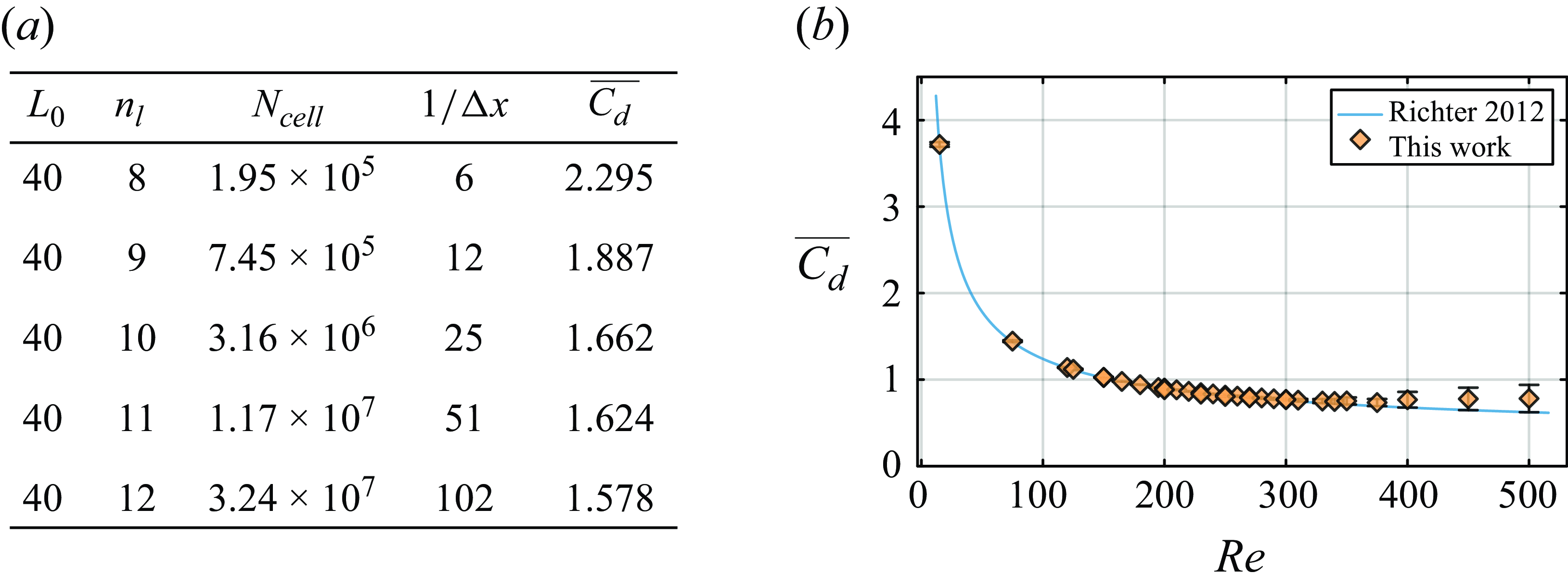
Figure 21. (a) Mesh convergence of $\overline {C_d}$
in the flow past a fixed tetrahedron at
$\overline {C_d}$
in the flow past a fixed tetrahedron at ${{R}e} = 100$
with grid refinement.
${{R}e} = 100$
with grid refinement. $L_0$
denotes the dimensionless domain size,
$L_0$
denotes the dimensionless domain size, $n_l$
the adaptive grid refinement level,
$n_l$
the adaptive grid refinement level, $N_{cell}$
the total number of cells and
$N_{cell}$
the total number of cells and $1/\Delta x$
the number of cells per equivalent diameter. (b) Validation of
$1/\Delta x$
the number of cells per equivalent diameter. (b) Validation of $\overline {C_d}$
as a function of
$\overline {C_d}$
as a function of ${R}e$
in the flow past a fixed cube with a face facing the flow, compared with Richter & Nikrityuk (Reference Richter and Nikrityuk2012).
${R}e$
in the flow past a fixed cube with a face facing the flow, compared with Richter & Nikrityuk (Reference Richter and Nikrityuk2012).
Furthermore, we perform a series of simulations of the flow past a fixed cube with a square face facing the flow, covering a Reynolds number range of $1 \leqslant {{R}e} \leqslant 500$
. The results are presented in figure 21(b). For reference, we use the correlation provided by Richter & Nikrityuk (Reference Richter and Nikrityuk2012), which offers values of
$1 \leqslant {{R}e} \leqslant 500$
. The results are presented in figure 21(b). For reference, we use the correlation provided by Richter & Nikrityuk (Reference Richter and Nikrityuk2012), which offers values of $\overline {C_d}$
for laminar flow past a fixed cube within the range
$\overline {C_d}$
for laminar flow past a fixed cube within the range $10 \leqslant {{R}e} \leqslant 250$
. The grid resolution for these simulations is set to
$10 \leqslant {{R}e} \leqslant 250$
. The grid resolution for these simulations is set to $(n_l=12, 1/\Delta x=102)$
. Figure 21(b) shows excellent agreement between our numerical results with Richter’s correlation (relative error
$(n_l=12, 1/\Delta x=102)$
. Figure 21(b) shows excellent agreement between our numerical results with Richter’s correlation (relative error $\varepsilon \lt 1\,\%$
) for
$\varepsilon \lt 1\,\%$
) for $10 \leqslant \textit{Re} \leqslant 300$
. For
$10 \leqslant \textit{Re} \leqslant 300$
. For $300 \leqslant {{R}e} \leqslant 500$
, higher relative errors (
$300 \leqslant {{R}e} \leqslant 500$
, higher relative errors ( $1\,\% \lt \varepsilon \lt 10\,\%$
) are observed. However, note that Richter’s correlation is valid for
$1\,\% \lt \varepsilon \lt 10\,\%$
) are observed. However, note that Richter’s correlation is valid for $10 \leqslant {{R}e} \leqslant 250$
and has not been verified beyond this range. Additionally, the trend in
$10 \leqslant {{R}e} \leqslant 250$
and has not been verified beyond this range. Additionally, the trend in $\overline {C_d}(\textit{Re})$
– featuring a plateau around
$\overline {C_d}(\textit{Re})$
– featuring a plateau around ${{R}e} = 300 {-} 350$
followed by a slight increase – aligns well with numerical results from Seyed-Ahmadi & Wachs (Reference Seyed-Ahmadi and Wachs2019) and Meng et al. (Reference Meng, An, Cheng and Kimiaei2021) under similar flow conditions. Therefore, the relative errors compared with Richter’s correlation for
${{R}e} = 300 {-} 350$
followed by a slight increase – aligns well with numerical results from Seyed-Ahmadi & Wachs (Reference Seyed-Ahmadi and Wachs2019) and Meng et al. (Reference Meng, An, Cheng and Kimiaei2021) under similar flow conditions. Therefore, the relative errors compared with Richter’s correlation for ${{R}e} \gt 250$
are considered acceptable.
${{R}e} \gt 250$
are considered acceptable.
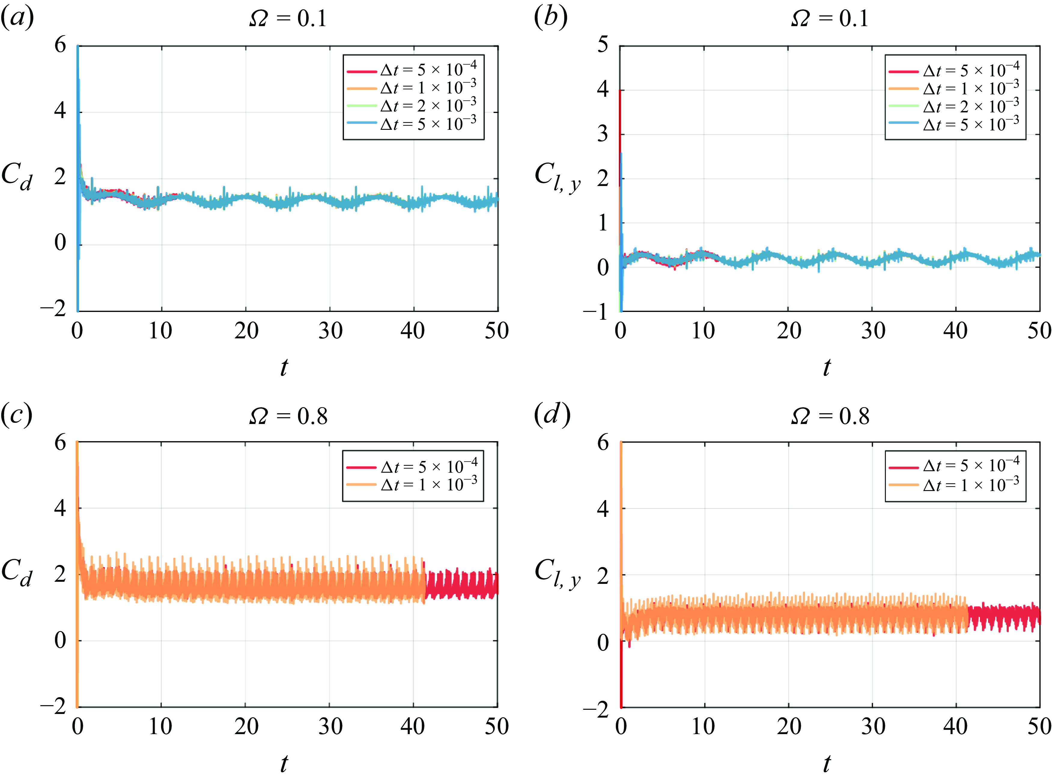
Figure 22. Temporal evolution of $C_d$
and
$C_d$
and $C_{l,y}$
of the rotating RCF4 cube at: (a,b)
$C_{l,y}$
of the rotating RCF4 cube at: (a,b) ${{R}e}=100$
and
${{R}e}=100$
and $\Omega =0.1$
, with increasing time step magnitude from
$\Omega =0.1$
, with increasing time step magnitude from $\Delta t = 5\times 10^{-4}$
to
$\Delta t = 5\times 10^{-4}$
to $5\times 10^{-3}$
; (c,d)
$5\times 10^{-3}$
; (c,d) ${{R}e}=100$
and
${{R}e}=100$
and $\Omega =0.8$
, from
$\Omega =0.8$
, from $\Delta t = 5\times 10^{-4}$
to
$\Delta t = 5\times 10^{-4}$
to $1\times 10^{-3}$
.
$1\times 10^{-3}$
.
Accurate simulations of particle–flow interactions for a rotating angular particle requires careful choice of time resolution. In figure 22, we show the evolution of $C_d$
and
$C_d$
and $C_{l,y}$
for a transversely rotating cube (RCF4) in the flow at
$C_{l,y}$
for a transversely rotating cube (RCF4) in the flow at ${{R}e}=100$
. Two scenarios must be considered separately: (i) for a slowly rotating particle,
${{R}e}=100$
. Two scenarios must be considered separately: (i) for a slowly rotating particle, $\Delta t$
needs to be large enough to capture a sufficient number of periods to accurately compute time-averaged physical quantities; (ii) for a rapidly rotating particle, a smaller
$\Delta t$
needs to be large enough to capture a sufficient number of periods to accurately compute time-averaged physical quantities; (ii) for a rapidly rotating particle, a smaller $\Delta t$
is necessary to ensure enough frames within a single period, thereby avoiding unphysical oscillatory signals.
$\Delta t$
is necessary to ensure enough frames within a single period, thereby avoiding unphysical oscillatory signals.
In figures 22(a) and 22(b), we present the temporal evolution of $C_d$
and
$C_d$
and $C_{l,y}$
for RCF4 at
$C_{l,y}$
for RCF4 at $\Omega =0.1$
. At this rotation rate, we observe that all four curves overlap as the time step increases from
$\Omega =0.1$
. At this rotation rate, we observe that all four curves overlap as the time step increases from $\Delta t = 5\times 10^{-4}$
to
$\Delta t = 5\times 10^{-4}$
to $\Delta t = 5\times 10^{-3}$
. A similar pattern is observed for lower rotation rates,
$\Delta t = 5\times 10^{-3}$
. A similar pattern is observed for lower rotation rates, $\Omega \leqslant 0.1$
. Therefore, we select
$\Omega \leqslant 0.1$
. Therefore, we select $\Delta t=5\times 10^{-3}$
as the maximum time step for these simulations. At higher rotation rates, such as
$\Delta t=5\times 10^{-3}$
as the maximum time step for these simulations. At higher rotation rates, such as $\Omega =0.8$
, we plot the temporal evolution of
$\Omega =0.8$
, we plot the temporal evolution of $C_d$
and
$C_d$
and $C_{l,y}$
in figures 22(c) and 22(d). For these cases, a smaller time step is necessary, and we find that
$C_{l,y}$
in figures 22(c) and 22(d). For these cases, a smaller time step is necessary, and we find that $\Delta t=5\times 10^{-4}$
closely matches the behaviour observed with
$\Delta t=5\times 10^{-4}$
closely matches the behaviour observed with $\Delta t = 1\times 10^{-3}$
for both
$\Delta t = 1\times 10^{-3}$
for both $C_d$
and
$C_d$
and $C_{l,y}$
. To achieve the best resolution in our simulations, we choose
$C_{l,y}$
. To achieve the best resolution in our simulations, we choose $\Delta t=5\times 10^{-4}$
as maximal time step for fast rotating cases,
$\Delta t=5\times 10^{-4}$
as maximal time step for fast rotating cases, $\Omega \gt 0.1$
. The time step selection in the simulations is adaptive and dynamic, carefully adjusted to satisfy the CFL condition. A more detailed and complete strategy for this approach is provided in (2.15).
$\Omega \gt 0.1$
. The time step selection in the simulations is adaptive and dynamic, carefully adjusted to satisfy the CFL condition. A more detailed and complete strategy for this approach is provided in (2.15).
Consequently, the chosen spatial and time resolutions for this study have been reliably validated, ensuring that the generated data set is free from significant biases due to computational spatial and temporal errors.
Appendix C. Vortex shedding and wake structures of RCF4
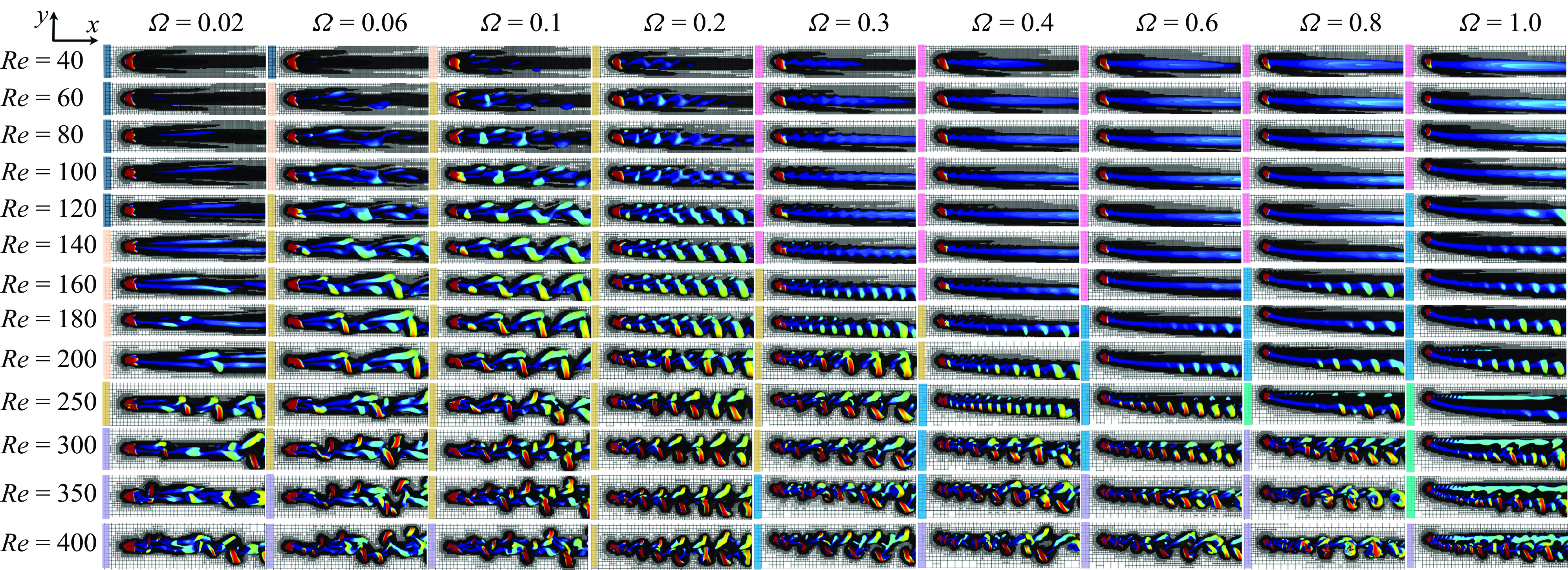
Figure 23. Vortex shedding and suppression in the wake of the rotating RCF4 cube in the $x$
-
$x$
- $y$
plane at
$y$
plane at $0.02 \leqslant \Omega \leqslant 1$
and
$0.02 \leqslant \Omega \leqslant 1$
and $40\leqslant {{R}e}\leqslant 400$
. Isosurfaces are identified using the criterion
$40\leqslant {{R}e}\leqslant 400$
. Isosurfaces are identified using the criterion $\lambda _2 = -1$
, and coloured by streamwise velocity
$\lambda _2 = -1$
, and coloured by streamwise velocity $u_x$
, with red indicating high velocity and blue indicating low velocity.
$u_x$
, with red indicating high velocity and blue indicating low velocity.
To provide a comprehensive view of regime transitions, figure 23 presents the vortical structures identified by $\lambda _2 = -1$
in the
$\lambda _2 = -1$
in the $x$
-
$x$
- $y$
plane for most cases of RCF4 investigated in this study, spanning
$y$
plane for most cases of RCF4 investigated in this study, spanning $40 \leqslant {{R}e} \leqslant 400$
and
$40 \leqslant {{R}e} \leqslant 400$
and $0.02 \leqslant \Omega \leqslant 1$
. The vortical structures are coloured by
$0.02 \leqslant \Omega \leqslant 1$
. The vortical structures are coloured by $u_x$
. The colour-coded boxes to the left of each case indicate the corresponding regimes, matching the regimes in figure 4. This vortex-shedding map illustrates the effects of varying
$u_x$
. The colour-coded boxes to the left of each case indicate the corresponding regimes, matching the regimes in figure 4. This vortex-shedding map illustrates the effects of varying ${R}e$
and
${R}e$
and $\Omega$
on the wake instability. At low
$\Omega$
on the wake instability. At low $\Omega$
and
$\Omega$
and ${R}e$
, the wake exhibits steady, straight or fragmented vortical structures. As both parameters increase, the flow becomes progressively more unsteady, with periodic vortex shedding patterns emerging in the HS regime. Vortex suppression is observed at
${R}e$
, the wake exhibits steady, straight or fragmented vortical structures. As both parameters increase, the flow becomes progressively more unsteady, with periodic vortex shedding patterns emerging in the HS regime. Vortex suppression is observed at ${{R}e} \leqslant 140$
and
${{R}e} \leqslant 140$
and $\Omega \geqslant 0.3$
for RCF4. As
$\Omega \geqslant 0.3$
for RCF4. As ${R}e$
and
${R}e$
and $\Omega$
further increase, the previously suppressed wake becomes unsteady again, transitioning to the HS, KH and DS regimes. At
$\Omega$
further increase, the previously suppressed wake becomes unsteady again, transitioning to the HS, KH and DS regimes. At ${{R}e} \geqslant 400$
, the flow generally transitions to a chaotic state, with the exception of the cases at
${{R}e} \geqslant 400$
, the flow generally transitions to a chaotic state, with the exception of the cases at $\Omega = 0.2$
and
$\Omega = 0.2$
and $\Omega = 0.3$
.
$\Omega = 0.3$
.
Appendix D. Length and volume of recirculation region
In the study of flow past a fixed angular particle, the length, shape and size of the recirculation region play crucial roles in determining the pattern and frequency of vortex shedding, which significantly influence wake instability (Gai & Wachs Reference Gai and Wachs2023b ). For rotating angular particles, this becomes even more pronounced, as the added rotational motion introduces complex interactions between the flow and the geometry of the particle, further impacting the structure and behaviour of the wake.
We define the recirculation region as the region where the streamwise velocity $u_x$
is less than or equal to zero. Its volume is given by
$u_x$
is less than or equal to zero. Its volume is given by
 \begin{equation} V_r = \int _{\Omega } H(-u_x) \, dV = \sum _{i,j,k} \mathcal{H}(-u_x(i,j,k)) \Delta V, \end{equation}
where $u_x(i,j,k)$
is the streamwise velocity at the grid cell located at indices
$u_x(i,j,k)$
is the streamwise velocity at the grid cell located at indices $(i,j,k)$
. Here,
$(i,j,k)$
. Here, $H(-u_x(i,j,k))$
is the discrete Heaviside function, which equals
$H(-u_x(i,j,k))$
is the discrete Heaviside function, which equals $1$
if
$1$
if $u_x(i,j,k) \leqslant 0$
, indicating flow reversal in that cell, and
$u_x(i,j,k) \leqslant 0$
, indicating flow reversal in that cell, and $0$
otherwise. Additionally,
$0$
otherwise. Additionally, $\Delta V = \Delta V^*/V^*_{sph}$
is the dimensionless volume of a single grid cell. Since the angular position of the rotating angular particles keeps changing in time, we define
$\Delta V = \Delta V^*/V^*_{sph}$
is the dimensionless volume of a single grid cell. Since the angular position of the rotating angular particles keeps changing in time, we define $L_r$
as the
$L_r$
as the $x$
-component of the displacement from the particle centroid to the grid cell with the largest
$x$
-component of the displacement from the particle centroid to the grid cell with the largest $x$
-coordinate where the streamwise velocity component satisfies
$x$
-coordinate where the streamwise velocity component satisfies $u_x(i,j,k) \leqslant 0$
. Mathematically, it can be expressed as
$u_x(i,j,k) \leqslant 0$
. Mathematically, it can be expressed as
 \begin{equation} L_r =(\max \left ( x_{i} \mid u_x(i,j,k) \leqslant 0 \right ) - x_p), \end{equation}
where $x_p = x_p^*/D^*_{sph}$
is the dimensionless
$x_p = x_p^*/D^*_{sph}$
is the dimensionless $x$
-coordinate of the particle centroid.
$x$
-coordinate of the particle centroid.
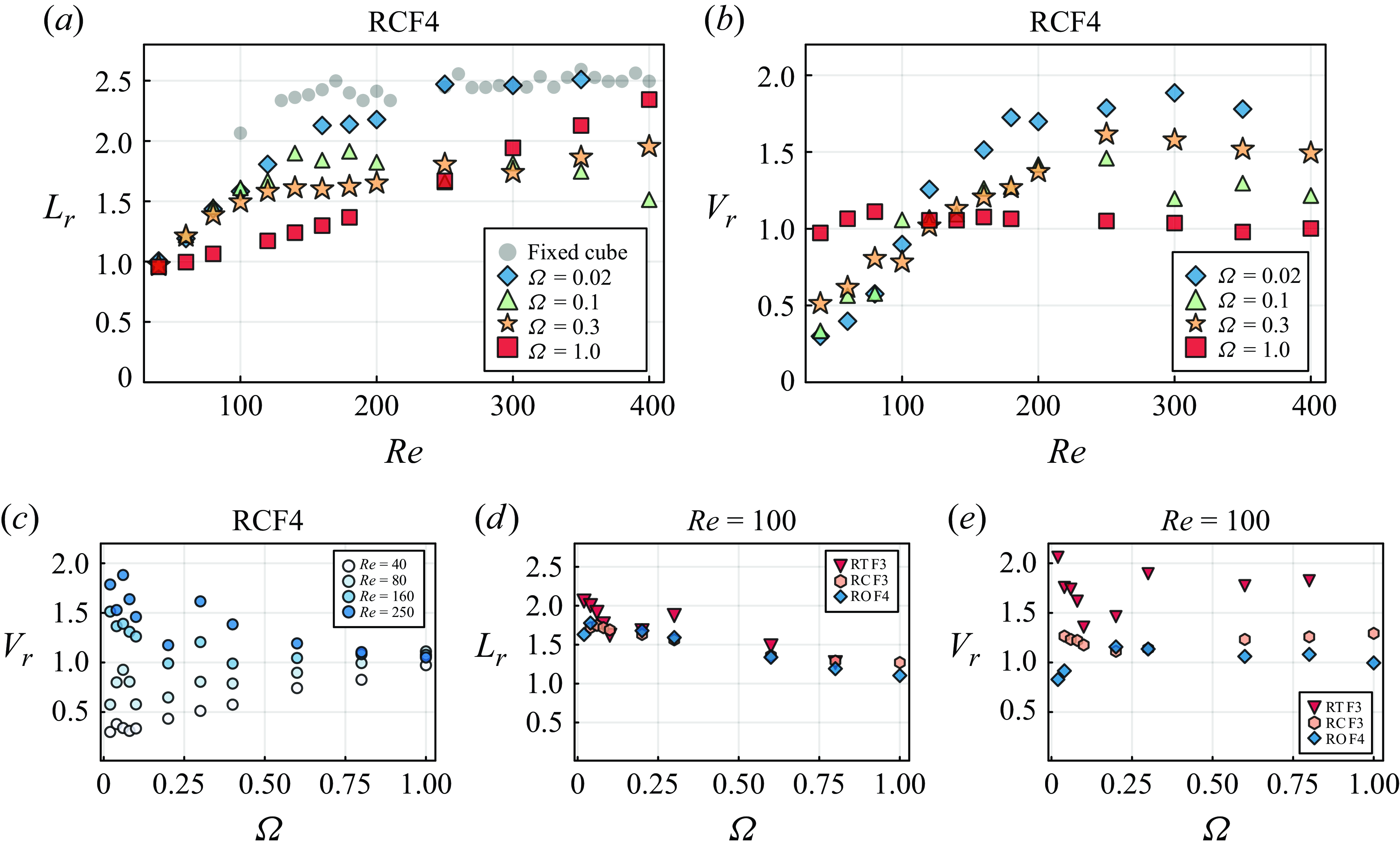
Figure 24. Evolution of recirculation region length $L_r$
and volume
$L_r$
and volume $V_r$
in the wake of a transversely rotating angular particle. RCF4: (a)
$V_r$
in the wake of a transversely rotating angular particle. RCF4: (a) $L_r$
as a function of
$L_r$
as a function of ${R}e$
for increasing
${R}e$
for increasing $\Omega$
, with reference values of the flow past a fixed cube plotted as grey dots; (b)
$\Omega$
, with reference values of the flow past a fixed cube plotted as grey dots; (b) $V_r$
as a function of
$V_r$
as a function of ${R}e$
for different
${R}e$
for different $\Omega$
; (c)
$\Omega$
; (c) $V_r$
as a function of
$V_r$
as a function of $\Omega$
for different
$\Omega$
for different ${R}e$
. The effects of particle angularity on
${R}e$
. The effects of particle angularity on $L_r$
and
$L_r$
and $V_r$
as a function of
$V_r$
as a function of $\Omega$
are depicted in panels (d) and (e), respectively.
$\Omega$
are depicted in panels (d) and (e), respectively.
We begin with RCF4 and then discuss the effects of particle angularity, as shown in figure 24. From figure 24(a), we observe that $L_r$
of RCF4 increases with flow inertia for
$L_r$
of RCF4 increases with flow inertia for $40 \leqslant {{R}e} \leqslant 400$
. At
$40 \leqslant {{R}e} \leqslant 400$
. At ${{R}e} \leqslant 200$
, higher
${{R}e} \leqslant 200$
, higher $\Omega$
results in a shorter
$\Omega$
results in a shorter $L_r$
. For
$L_r$
. For ${{R}e} \geqslant 250$
, at
${{R}e} \geqslant 250$
, at $\Omega = 0.02$
, the effects of rotation are minimal, with
$\Omega = 0.02$
, the effects of rotation are minimal, with $L_r$
values closely matching those of the fixed cube case in grey circles. However, as
$L_r$
values closely matching those of the fixed cube case in grey circles. However, as $\Omega$
increases, the trend becomes less obvious. Regarding the volume of the recirculation region, figure 24(b) shows that
$\Omega$
increases, the trend becomes less obvious. Regarding the volume of the recirculation region, figure 24(b) shows that $V_r$
increases with
$V_r$
increases with ${R}e$
before reaching a plateau. For
${R}e$
before reaching a plateau. For ${{R}e} \leqslant 100$
, higher
${{R}e} \leqslant 100$
, higher $\Omega$
results in a larger
$\Omega$
results in a larger $V_r$
. The slow-rotating cube at
$V_r$
. The slow-rotating cube at $\Omega = 0.02$
continues to exhibit an increase in
$\Omega = 0.02$
continues to exhibit an increase in $V_r$
for
$V_r$
for ${{R}e} \geqslant 100$
. Interestingly, for the fast-rotating cube at
${{R}e} \geqslant 100$
. Interestingly, for the fast-rotating cube at $\Omega = 1$
,
$\Omega = 1$
, $V_r$
remains approximately constant at
$V_r$
remains approximately constant at $V_r \approx 1$
across the range
$V_r \approx 1$
across the range $40 \leqslant {{R}e} \leqslant 400$
. Additionally, for
$40 \leqslant {{R}e} \leqslant 400$
. Additionally, for ${{R}e} \geqslant 250$
, we observe that
${{R}e} \geqslant 250$
, we observe that $V_r$
at
$V_r$
at $\Omega = 0.3$
is larger than that at
$\Omega = 0.3$
is larger than that at $\Omega = 0.1$
, which can be attributed to the regime transition from the HS regime to the VS regime. This behaviour is further clarified in figure 24(c), where
$\Omega = 0.1$
, which can be attributed to the regime transition from the HS regime to the VS regime. This behaviour is further clarified in figure 24(c), where $V_r$
is plotted as a function of
$V_r$
is plotted as a function of $\Omega$
for several selected values of
$\Omega$
for several selected values of ${R}e$
. It is important to note that even though the vortex within the recirculation region disappears in the VS regime, as observed in the rotating sphere case (Giacobello et al. Reference Giacobello, Ooi and Balachandar2009), the recirculation volume
${R}e$
. It is important to note that even though the vortex within the recirculation region disappears in the VS regime, as observed in the rotating sphere case (Giacobello et al. Reference Giacobello, Ooi and Balachandar2009), the recirculation volume $V_r$
, as defined in (D1), is not zero. Two key insights emerge from this figure: (i)
$V_r$
, as defined in (D1), is not zero. Two key insights emerge from this figure: (i) $V_r$
exhibits a local minimum at
$V_r$
exhibits a local minimum at $\Omega =0.2$
, which corresponds to high-frequency vortex shedding, leading to a local maximum of the drag coefficient
$\Omega =0.2$
, which corresponds to high-frequency vortex shedding, leading to a local maximum of the drag coefficient $C_d$
, as shown in figure 12(a); (ii) as
$C_d$
, as shown in figure 12(a); (ii) as $\Omega$
increases,
$\Omega$
increases, $V_r$
converges to a value of approximately
$V_r$
converges to a value of approximately $1$
, regardless of the flow inertia. The rotational motion of the cube becomes dominant over the flow inertia, leading to a constant
$1$
, regardless of the flow inertia. The rotational motion of the cube becomes dominant over the flow inertia, leading to a constant $V_r$
. Yang et al. (Reference Yang, Wang, Guo and Zhang2023) also observed that
$V_r$
. Yang et al. (Reference Yang, Wang, Guo and Zhang2023) also observed that $L_r$
becomes less sensitive to variations in
$L_r$
becomes less sensitive to variations in ${R}e$
for flow past a rotating short cylinder.
${R}e$
for flow past a rotating short cylinder.
We further examine the effects of $\phi$
on
$\phi$
on $L_r$
in figure 24(d), focusing on the RTF3, RCF3 and ROF4 cases. Since the three angular particles have the same volume,
$L_r$
in figure 24(d), focusing on the RTF3, RCF3 and ROF4 cases. Since the three angular particles have the same volume, $L_r$
exhibits a similar decreasing trend with increasing
$L_r$
exhibits a similar decreasing trend with increasing $\Omega$
. This occurs because, as
$\Omega$
. This occurs because, as $\Omega$
increases, the recirculation region shifts towards the lower part of the particle, reducing its extent in the streamwise direction. Similar results were reported for flow past a rotating short cylinder, where the decrease in
$\Omega$
increases, the recirculation region shifts towards the lower part of the particle, reducing its extent in the streamwise direction. Similar results were reported for flow past a rotating short cylinder, where the decrease in $L_r$
at high
$L_r$
at high $\Omega$
was found to stabilise the flow (Yang et al. Reference Yang, Wang, Guo and Zhang2023). RTF3 shows slightly higher
$\Omega$
was found to stabilise the flow (Yang et al. Reference Yang, Wang, Guo and Zhang2023). RTF3 shows slightly higher $L_r$
values in the slow-rotating regimes (for example,
$L_r$
values in the slow-rotating regimes (for example, $\Omega \leqslant 0.08$
) than those of the other two particles. However,
$\Omega \leqslant 0.08$
) than those of the other two particles. However, $V_r$
increases clearly with the particle angularity, i.e. as
$V_r$
increases clearly with the particle angularity, i.e. as $\phi$
decreases. In figure 24(e), we note that RTF3 consistently exhibits larger
$\phi$
decreases. In figure 24(e), we note that RTF3 consistently exhibits larger $V_r$
than those of RCF3 and ROF4 throughout the range
$V_r$
than those of RCF3 and ROF4 throughout the range $0.02 \leqslant \Omega \leqslant 1$
. A local minimum in
$0.02 \leqslant \Omega \leqslant 1$
. A local minimum in $V_r$
around
$V_r$
around $\Omega \approx 0.2$
is observed for both RTF3 and RCF3.
$\Omega \approx 0.2$
is observed for both RTF3 and RCF3.
Appendix E. Correlations for
$C_d$
and
$C_{\Omega }$
at
${{R}e} \leqslant 200$


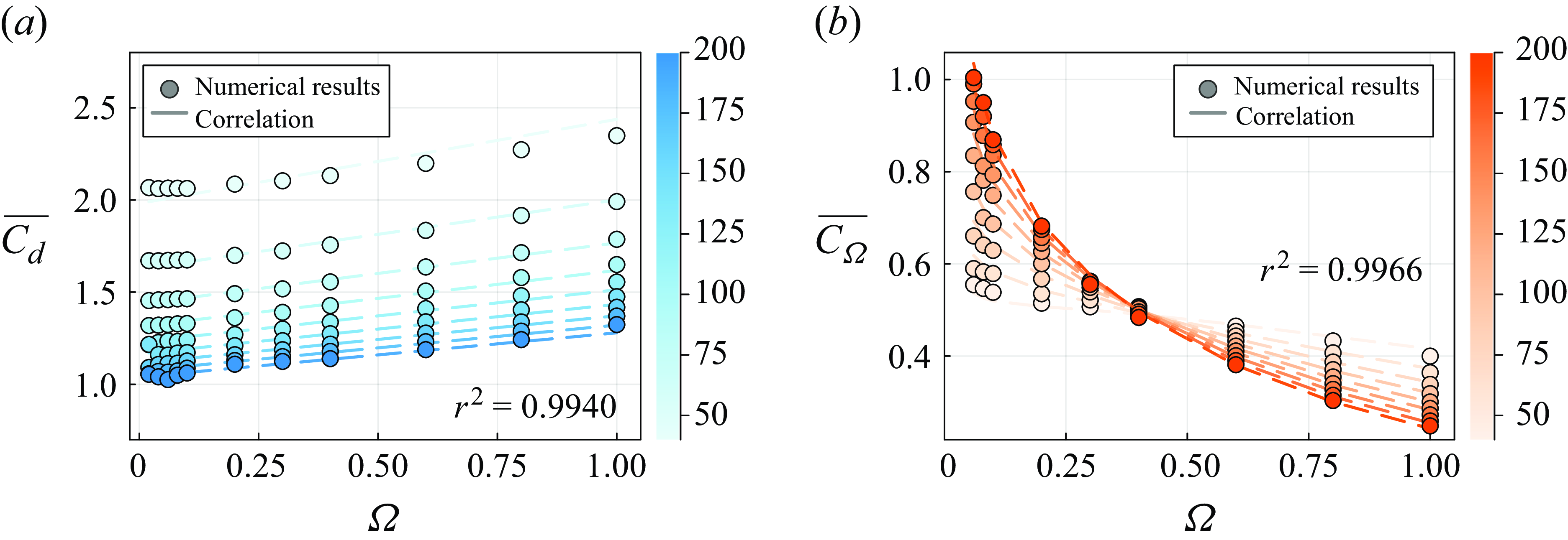
Figure 25. (a) Evolution of the time-averaged drag coefficient $\overline {C_{d}}$
of the rotating RCF4 cube as a function of
$\overline {C_{d}}$
of the rotating RCF4 cube as a function of $\Omega$
at
$\Omega$
at $40 \leqslant {{R}e} \leqslant 200$
with increment
$40 \leqslant {{R}e} \leqslant 200$
with increment $\Delta {{R}e}=20$
. (b) Evolution of
$\Delta {{R}e}=20$
. (b) Evolution of $\overline {C_{\Omega }}$
at
$\overline {C_{\Omega }}$
at $40 \leqslant {{R}e} \leqslant 200$
with increment
$40 \leqslant {{R}e} \leqslant 200$
with increment $\Delta {{R}e}=20$
and
$\Delta {{R}e}=20$
and $0.06 \leqslant \Omega \leqslant 1$
. Our numerical simulation results (coloured circles) are compared with the empirical correlations from (E1) for
$0.06 \leqslant \Omega \leqslant 1$
. Our numerical simulation results (coloured circles) are compared with the empirical correlations from (E1) for $C_d$
and (E2) for
$C_d$
and (E2) for $C_{\Omega }$
, shown by dashed lines. Darker circles indicate higher values of
$C_{\Omega }$
, shown by dashed lines. Darker circles indicate higher values of ${R}e$
.
${R}e$
.
The drag coefficient plays a central role in fluid–particle interactions. However, existing correlations in the literature are typically derived for spheres or stationary particles, and thus fail to account for the added complexity introduced by angular particle rotation. For rotating cubes – like the RCF4 cube – the flow separation, wake structure and drag force differ significantly from spheres. Therefore, developing a new empirical correlation to the rotating cube is crucial for accurately modelling drag forces in CFD–DEM simulations.
Similarly to the $\overline {C_{l,y}}$
correlation, we derive an empirical correlation for
$\overline {C_{l,y}}$
correlation, we derive an empirical correlation for $\overline {C_d}$
based on our numerical dataset within the range
$\overline {C_d}$
based on our numerical dataset within the range $40 \leqslant {{R}e} \leqslant 200$
. To capture the influence of particle rotation, we introduce a correction factor to the classical drag correlation proposed by Schiller & Naumann (Reference Schiller and Naumann1935). Using multivariate regression, we determine the coefficients of each term and propose the following new correlation:
$40 \leqslant {{R}e} \leqslant 200$
. To capture the influence of particle rotation, we introduce a correction factor to the classical drag correlation proposed by Schiller & Naumann (Reference Schiller and Naumann1935). Using multivariate regression, we determine the coefficients of each term and propose the following new correlation:
 \begin{equation} \displaystyle {\overline {C_d} = \frac {24}{\textit{Re}}(1 + 0.0628{{R}e}^{0.833})(1.401 + 0.323 \Omega )}, \end{equation}
In this expression, the first term represents the Stokes drag, the second term accounts for inertial corrections and the third term captures the influence of cube rotation. A direct comparison with our numerical results is shown in figure 25(a) for varying $\Omega$
across the range of Reynolds number
$\Omega$
across the range of Reynolds number $40 \leqslant {{R}e} \leqslant 200$
. The near-linear increase of
$40 \leqslant {{R}e} \leqslant 200$
. The near-linear increase of $\overline {C_d}$
with
$\overline {C_d}$
with $\Omega$
is accurately captured by the third term in (E1), while the decrease of
$\Omega$
is accurately captured by the third term in (E1), while the decrease of $\overline {C_d}$
with increasing
$\overline {C_d}$
with increasing ${R}e$
is also well represented. Overall, the proposed correlation in (E1) exhibits excellent agreement with the numerical results, achieving a coefficient of determination
${R}e$
is also well represented. Overall, the proposed correlation in (E1) exhibits excellent agreement with the numerical results, achieving a coefficient of determination $R^2 = 0.9940$
.
$R^2 = 0.9940$
.
As discussed in § 4.4.3, the rotation coefficient $C_{\Omega }$
is of vital importance in force balance and trajectory instability analyses of freely moving particles. However, few studies have developed correlations for this important coefficient, especially in the context of rotating angular particles. To address this gap, we introduce a novel empirical correlation for
$C_{\Omega }$
is of vital importance in force balance and trajectory instability analyses of freely moving particles. However, few studies have developed correlations for this important coefficient, especially in the context of rotating angular particles. To address this gap, we introduce a novel empirical correlation for $\overline {C_{\Omega }}$
as a function of
$\overline {C_{\Omega }}$
as a function of $\Omega$
and
$\Omega$
and ${R}e$
, derived from our numerical dataset:
${R}e$
, derived from our numerical dataset:
 \begin{equation} \displaystyle {\overline {C_{\Omega }} = (0.0817 + 0.59\Omega )(4.75 + 0.17{{R}e})\exp (-\Omega ^{0.409}{{R}e}^{0.291})}. \end{equation}
This expression consists of two multiplicative factors accounting separately for the effects of flow inertia and particle rotation, followed by an exponential term that captures their coupling. Figure 25(b) compares the correlation and numerical results of $\overline {C_{\Omega }}$
for
$\overline {C_{\Omega }}$
for $40 \leqslant {{R}e} \leqslant 200$
. The correlation accurately reflects the influences of both
$40 \leqslant {{R}e} \leqslant 200$
. The correlation accurately reflects the influences of both ${R}e$
and
${R}e$
and $\Omega$
, achieving an overall coefficient of determination
$\Omega$
, achieving an overall coefficient of determination $R^2 = 0.9966$
. In addition, the invariance region of
$R^2 = 0.9966$
. In addition, the invariance region of $\overline {C_{\Omega }}$
with respect to
$\overline {C_{\Omega }}$
with respect to ${R}e$
at
${R}e$
at $\Omega = 0.3 {-} 0.4$
is well captured by the balance between the linear term
$\Omega = 0.3 {-} 0.4$
is well captured by the balance between the linear term $4.75 + 0.17\,{{R}e}$
and the exponential term
$4.75 + 0.17\,{{R}e}$
and the exponential term $\exp \bigl (-\Omega ^{0.409}\,{{R}e}^{0.291}\bigr )$
in (E2).
$\exp \bigl (-\Omega ^{0.409}\,{{R}e}^{0.291}\bigr )$
in (E2).
Appendix F. Hydrodynamic torque on the rotating angular particle
In addition to drag and lift forces, hydrodynamic torques are instrumental in determining the trajectories of freely moving particles. They alter particle angular positions, rotation velocities and thereby affect the Magnus effect, which is particularly significant for non-spherical particles (Fernandes et al. Reference Fernandes, Ern, Risso and Magnaudet2008; Ern et al. Reference Ern, Risso, Fernandes and Magnaudet2009; Gai & Wachs Reference Gai and Wachs2024).
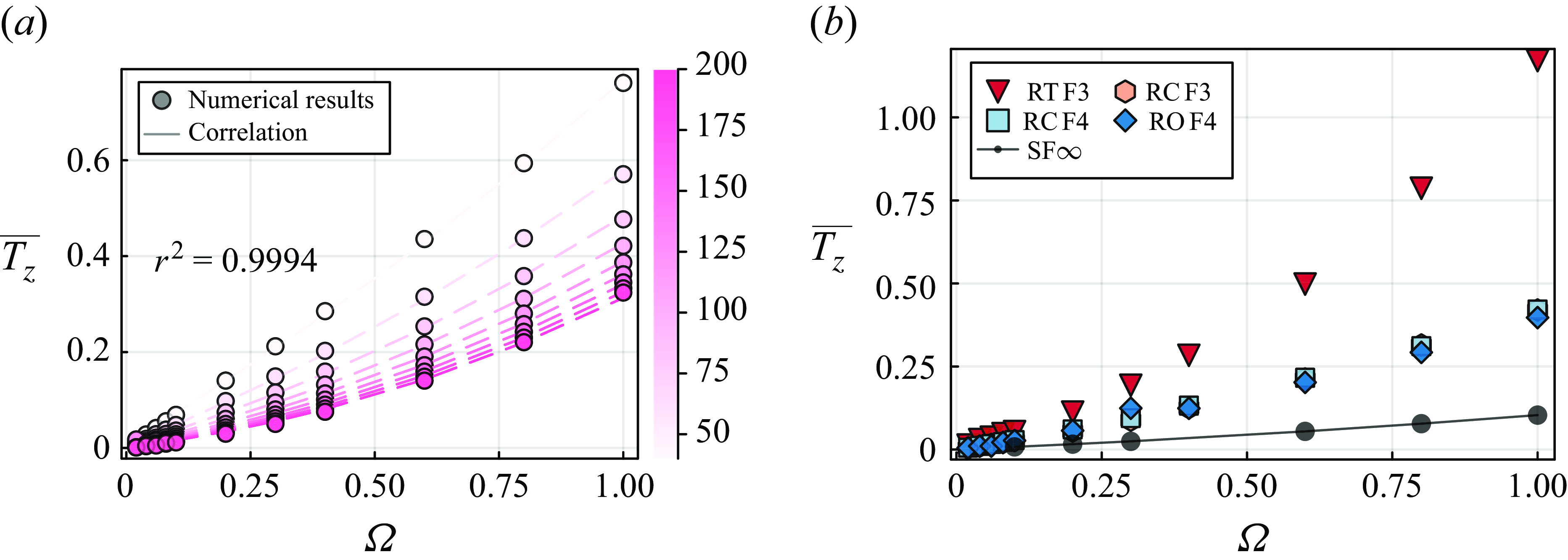
Figure 26. (a) Time-averaged torque $\overline {T_z}$
of the rotating RCF4 cube as a function of
$\overline {T_z}$
of the rotating RCF4 cube as a function of $0.02 \leqslant \Omega \leqslant 1$
at
$0.02 \leqslant \Omega \leqslant 1$
at $40 \leqslant {{R}e} \leqslant 200$
. The increasing darkness of the circles represents higher
$40 \leqslant {{R}e} \leqslant 200$
. The increasing darkness of the circles represents higher ${R}e$
. For comparison, the empirical correlation in (F1) is illustrated by the dashed lines. (b) Effects of particle angularity on the
${R}e$
. For comparison, the empirical correlation in (F1) is illustrated by the dashed lines. (b) Effects of particle angularity on the $\overline {T_z}$
exerted on a rotating particle at
$\overline {T_z}$
exerted on a rotating particle at ${{R}e}=100$
. The case of a rotating sphere (
${{R}e}=100$
. The case of a rotating sphere ( $RSF\infty$
) at
$RSF\infty$
) at ${{R}e}=100$
is provided as a reference and shown by the black solid line with circles.
${{R}e}=100$
is provided as a reference and shown by the black solid line with circles.
We thoroughly examine and present the evolution of the time-averaged torque, $\overline {T_z}$
, using (2.6) for a rotating RCF4 cube at
$\overline {T_z}$
, using (2.6) for a rotating RCF4 cube at $40 \leqslant {{R}e} \leqslant 200$
, as shown in figure 26(a). Since
$40 \leqslant {{R}e} \leqslant 200$
, as shown in figure 26(a). Since $\Omega$
is imposed and held constant,
$\Omega$
is imposed and held constant, $\overline {T_z}$
reflects the hydrodynamic response of the fluid to the rotating particle. Clearly,
$\overline {T_z}$
reflects the hydrodynamic response of the fluid to the rotating particle. Clearly, $\overline {T_z}$
increases with
$\overline {T_z}$
increases with $\Omega$
. At higher
$\Omega$
. At higher ${R}e$
, flow inertia dominates over viscous forces, resulting in a thinner boundary layer and reduced shear stresses that generate torque. Moreover, the decrease of
${R}e$
, flow inertia dominates over viscous forces, resulting in a thinner boundary layer and reduced shear stresses that generate torque. Moreover, the decrease of $\overline {T_z}$
is less pronounced with increasing flow inertia to
$\overline {T_z}$
is less pronounced with increasing flow inertia to $200 \leqslant {{R}e} \leqslant 400$
(data not shown for brevity). To better understand the coupling between
$200 \leqslant {{R}e} \leqslant 400$
(data not shown for brevity). To better understand the coupling between ${R}e$
and
${R}e$
and $\Omega$
and their overall effect on
$\Omega$
and their overall effect on $\overline {T_z}$
, we establish a simple scaling relation for
$\overline {T_z}$
, we establish a simple scaling relation for $\overline {T_z}$
as follows:
$\overline {T_z}$
as follows:
 \begin{equation} \displaystyle {\overline {T_z} = 0.2 \Omega ^2\left (1 + 4.743\Omega ^{-1.1}\frac {24}{{{R}e}}\right )}. \end{equation}
This relation matches the numerical results for $40 \leqslant {{R}e} \leqslant 200$
remarkably well, with
$40 \leqslant {{R}e} \leqslant 200$
remarkably well, with $R^2 = 0.9994$
as indicated in figure 26(a). It is interesting to note that for small
$R^2 = 0.9994$
as indicated in figure 26(a). It is interesting to note that for small ${R}e$
and
${R}e$
and $\Omega$
,
$\Omega$
, $\overline {T_z}$
scales with the Stokes drag factor
$\overline {T_z}$
scales with the Stokes drag factor $24/{{R}e}$
. In particular, as
$24/{{R}e}$
. In particular, as ${R}e$
approaches zero,
${R}e$
approaches zero, $\overline {T_z}$
varies linearly with
$\overline {T_z}$
varies linearly with $\Omega$
, a behaviour that is consistent with the observations in figure 26(a).
$\Omega$
, a behaviour that is consistent with the observations in figure 26(a).
How does $\overline {T_z}$
evolve for particles of different shapes? In figure 26(b), we compute and present
$\overline {T_z}$
evolve for particles of different shapes? In figure 26(b), we compute and present $\overline {T_z}$
for particles with varying angularities and rotational symmetry folds
$\overline {T_z}$
for particles with varying angularities and rotational symmetry folds $N_{\mathcal{F}}$
at
$N_{\mathcal{F}}$
at ${{R}e}=100$
. We observe that RTF3, which has high angularity (
${{R}e}=100$
. We observe that RTF3, which has high angularity ( $\phi =0.67$
), exhibits a higher value of
$\phi =0.67$
), exhibits a higher value of $\overline {T_z}$
than cubes (
$\overline {T_z}$
than cubes ( $\phi =0.806$
) and octahedrons (
$\phi =0.806$
) and octahedrons ( $\phi =0.846$
). The difference between RTF3 and the other angular particles becomes more pronounced with increasing
$\phi =0.846$
). The difference between RTF3 and the other angular particles becomes more pronounced with increasing $\Omega$
, reaching up to 2.8 times that of RCF4 at
$\Omega$
, reaching up to 2.8 times that of RCF4 at $\Omega =1$
. From figure 26(b), the difference between cubes and octahedrons are quite subtle. As a reference,
$\Omega =1$
. From figure 26(b), the difference between cubes and octahedrons are quite subtle. As a reference, $\overline {T_z}$
of a rotating sphere is also provided, and it is smaller than that of all angular particles. Overall, the particle angularity is a key factor playing a more significant role than the rotational symmetry fold
$\overline {T_z}$
of a rotating sphere is also provided, and it is smaller than that of all angular particles. Overall, the particle angularity is a key factor playing a more significant role than the rotational symmetry fold $N_{\mathcal{F}}$
on the evolution of
$N_{\mathcal{F}}$
on the evolution of $\overline {T_z}$
.
$\overline {T_z}$
.
Similar trends are also observed at ${{R}e}=60$
and
${{R}e}=60$
and $160$
(data not shown for brevity). Note that for these particles, the other two components of the hydrodynamic torque,
$160$
(data not shown for brevity). Note that for these particles, the other two components of the hydrodynamic torque, $\overline {T_x}$
and
$\overline {T_x}$
and $\overline {T_y}$
, are much smaller than
$\overline {T_y}$
, are much smaller than $\overline {T_z}$
at
$\overline {T_z}$
at $60 \leqslant {{R}e} \leqslant 160$
and are therefore not discussed. An exception is observed for RTF3, where the tetrahedron high angularity results in a non-negligible
$60 \leqslant {{R}e} \leqslant 160$
and are therefore not discussed. An exception is observed for RTF3, where the tetrahedron high angularity results in a non-negligible $\overline {T_x}$
, unlike the cases for the cube, octahedron or sphere. A comprehensive investigation of hydrodynamic torque components requires a wider range of particle shapes and axis of rotation to draw more general conclusions.
$\overline {T_x}$
, unlike the cases for the cube, octahedron or sphere. A comprehensive investigation of hydrodynamic torque components requires a wider range of particle shapes and axis of rotation to draw more general conclusions.


 Open access