


1. Introduction
1.1. Background
Incompressible multiphase flows are ubiquitous in nature, science and engineering, with a wide range of applications. (In this work, the term ‘phase’ denotes the different fluid materials/constituents (e.g. air and water)). The development of continuum models (and corresponding methods) that describe these flows has been an active field of research for the last few decades. This research can be (roughly) divided into (i) sharp interface models (Hirt & Nichols Reference Hirt and Nichols1981, Sethian Reference Sethian2001, ten Eikelder & Akkerman Reference ten Eikelder and Akkerman2021, Bothe Reference Bothe2022) and (ii) diffuse-interface models. Within the diffuse-interface category, phase-field models constitute a well-known class (Cahn & Hilliard Reference Cahn and Hilliard1958; Cahn Reference Cahn1959; Anderson, McFadden & Wheeler Reference Anderson, McFadden and Wheeler1998; Gomez & van der Zee Reference Gomez and van der Zee2018). While we acknowledge the importance of each of these approaches, the current article focuses on phase-field models.
Phase-field models have gained popularity over the last decades, and have become a versatile modelling technology with a wide range of applications in science and engineering. They offer resolutions to challenging moving-boundary problems by simultaneously addressing the geometrical representation and the physical model, see e.g. Anderson et al. (Reference Anderson, McFadden and Wheeler1998), Steinbach (Reference Steinbach2009). By representing interfaces implicitly through continuous field variables, phase-field models eliminate the need for explicit boundary tracking, enabling accurate and efficient simulations of phenomena such as solidification (Boettinger et al. Reference Boettinger, Warren, Beckermann and Karma2002), crack propagation in fracture mechanics (Ambati, Gerasimov & De Lorenzis Reference Ambati, Gerasimov and De Lorenzis2015) and two-fluid flow dynamics (Yue et al. Reference Yue, Feng, Liu and Shen2004).
The vast majority of incompressible, viscous, multiphase flow models in the literature is restricted to two fluids. In the realm of phase-field modelling, a prototypical model is the Navier–Stokes Cahn–Hilliard Allen–Cahn (NSCHAC) model. The first model of this kind, now known as model H, was proposed in Hohenberg & Halperin (Reference Hohenberg and Halperin1977). This model may be understood as a simplification of the more complete two-phase NSCHAC model in the sense that (i) it is restricted to matching fluid densities and (ii) it does not permit mass transfer between phases (i.e. it does not contain an Allen–Cahn-type term). The foundation of this model is based largely on empirical arguments; a derivation based on the concept of microforces (see Gurtin Reference Gurtin1996) was established in Gurtin, Polignone & Vinals (Reference Gurtin, Polignone and Vinals1996). In subsequent years, several efforts have been made to relax the matching-density restriction, see e.g. Lowengrub & Truskinovsky (Reference Lowengrub and Truskinovsky1998), Abels, Garcke & Grün (Reference Abels, Garcke and Grün2012), Aki et al. (Reference Aki, Dreyer, Giesselmann and Kraus2014), and see e.g. Kay & Welford (Reference Kay and Welford2007), Guo, Lin & Lowengrub (Reference Guo, Lin and Lowengrub2014), Khanwale et al. (Reference Khanwale, Saurabh, Fernando, Calo, Sundar, Rossmanith and Ganapathysubramanian2022), ten Eikelder & Schillinger (Reference ten Eikelder and Schillinger2024) for numerical simulations. Initially, these models were classified into two distinct categories: (i) models with a mass-averaged mixture velocity and (ii) models with a volume-averaged mixture velocity. In a recent article, we proposed a unified framework, rooted in continuum mixture theory, which leads to a single Navier–Stokes Cahn–Hilliard (NSCH) model that is invariant to the set of fundamental variables (ten Eikelder et al. Reference ten Eikelder, van der Zee, Akkerman and Schillinger2023); see ten Eikelder & Schillinger (Reference ten Eikelder and Schillinger2024) for a divergence-conforming discretisation with benchmarks. Contrary to the aforementioned classification, the framework indicates that the aforementioned classes of models coincide, up to minor modifications.
Although most research in the field of multiphase flows focuses on $N=2$
phases, there are various
$N=2$
phases, there are various $N$
-phase (
$N$
-phase ( $N\gt 2$
) incompressible flow models. Similar to the two-phase case, the literature on
$N\gt 2$
) incompressible flow models. Similar to the two-phase case, the literature on $N$
-phase models that (partly) utilise continuum mixture theory is divided into two categories: (i) models with a mass-averaged mixture velocity and (ii) models with a volume-averaged mixture velocity. Without attempting to be complete, we mention the
$N$
-phase models that (partly) utilise continuum mixture theory is divided into two categories: (i) models with a mass-averaged mixture velocity and (ii) models with a volume-averaged mixture velocity. Without attempting to be complete, we mention the $N$
-phase mass-averaged velocity models of Kim & Lowengrub (Reference Kim and Lowengrub2005) (
$N$
-phase mass-averaged velocity models of Kim & Lowengrub (Reference Kim and Lowengrub2005) ( $N=3$
) and Heida, Málek & Rajagopal (Reference Heida, Málek and Rajagopal2012), Li & Wang (Reference Li and Wang2014) (
$N=3$
) and Heida, Málek & Rajagopal (Reference Heida, Málek and Rajagopal2012), Li & Wang (Reference Li and Wang2014) ( $N\geqslant 2$
), and the
$N\geqslant 2$
), and the $N$
-phase volume-averaged models of Dong (Reference Dong2015, Reference Dong2018), Huang, Lin & Ardekani (Reference Huang, Lin and Ardekani2021) (
$N$
-phase volume-averaged models of Dong (Reference Dong2015, Reference Dong2018), Huang, Lin & Ardekani (Reference Huang, Lin and Ardekani2021) ( $N\geqslant 2$
). Furthermore, there are incompressible
$N\geqslant 2$
). Furthermore, there are incompressible $N$
-phase NSCH models that are not (partly) based on continuum mixture theory; rather, these models are established via coupling a multiphase Cahn–Hilliard (CH) model to the Navier–Stokes equations, see Boyer & Lapuerta (Reference Boyer and Lapuerta2006), Boyer et al. (Reference Boyer, Lapuerta, Minjeaud, Piar and Quintard2010), Tóth et al. (Reference Tóth, Pusztai and Gránásy2015), Zhang & Wang (Reference Zhang and Wang2016), Baňas & Nürnberg (Reference Baňas and Nürnberg2017), Xia, Kim & Li (Reference Xia, Kim and Li2022), Xiao et al. (Reference Xiao, Zeng, Zhang, Wang, Wang and Huang2024). We also refer to several theoretical considerations of Allen–Cahn/Cahn–Hilliard (AC/CH) systems in isolation (ignoring inertial phenomena present in fluid mechanic systems), see e.g. Eyre (Reference Eyre1993), Boyer & Minjeaud (Reference Boyer and Minjeaud2014), Tóth et al. (Reference Tóth, Pusztai and Gránásy2015), Li, Choi & Kim (Reference Li, Choi and Kim2016), Wu & Xu (Reference Wu and Xu2017), and to phase-field
$N$
-phase NSCH models that are not (partly) based on continuum mixture theory; rather, these models are established via coupling a multiphase Cahn–Hilliard (CH) model to the Navier–Stokes equations, see Boyer & Lapuerta (Reference Boyer and Lapuerta2006), Boyer et al. (Reference Boyer, Lapuerta, Minjeaud, Piar and Quintard2010), Tóth et al. (Reference Tóth, Pusztai and Gránásy2015), Zhang & Wang (Reference Zhang and Wang2016), Baňas & Nürnberg (Reference Baňas and Nürnberg2017), Xia, Kim & Li (Reference Xia, Kim and Li2022), Xiao et al. (Reference Xiao, Zeng, Zhang, Wang, Wang and Huang2024). We also refer to several theoretical considerations of Allen–Cahn/Cahn–Hilliard (AC/CH) systems in isolation (ignoring inertial phenomena present in fluid mechanic systems), see e.g. Eyre (Reference Eyre1993), Boyer & Minjeaud (Reference Boyer and Minjeaud2014), Tóth et al. (Reference Tóth, Pusztai and Gránásy2015), Li, Choi & Kim (Reference Li, Choi and Kim2016), Wu & Xu (Reference Wu and Xu2017), and to phase-field $N$
-phase flow models of Xia, Yang & Li (Reference Xia, Yang and Li2023), Mirjalili & Mani (Reference Mirjalili and Mani2024) that are not of NSCH type.
$N$
-phase flow models of Xia, Yang & Li (Reference Xia, Yang and Li2023), Mirjalili & Mani (Reference Mirjalili and Mani2024) that are not of NSCH type.
Although various $N$
-phase models have been proposed, their differences in assumptions and methodologies pose challenges for both theoretical analysis and practical application. A unified perspective remains elusive, complicating efforts to compare and refine these models.
$N$
-phase models have been proposed, their differences in assumptions and methodologies pose challenges for both theoretical analysis and practical application. A unified perspective remains elusive, complicating efforts to compare and refine these models.
1.2. Objective and main results
A number of the existing $N$
-phase phase-field models, already mentioned, and in the references therein, provide different models (alongside computational methodologies) for the same physical situation: the dynamics of viscous, incompressible (isothermal)
$N$
-phase phase-field models, already mentioned, and in the references therein, provide different models (alongside computational methodologies) for the same physical situation: the dynamics of viscous, incompressible (isothermal) $N$
-phase mixture flows. Naturally, there is some leeway in constitutive modelling, and not all models have the same complexity level. (To organise the various existing models one can adopt the classification introduced in Hutter & Jöhnk (Reference Hutter and Jöhnk2013)). This classification is for example utilised in Bothe & Dreyer (Reference Bothe and Dreyer2015), Hutter et al. (Reference Hutter, Wang, Hutter and Wang2018). However, one can infer that models within the same complexity class are already distinct before constitutive modelling. These observations raise questions regarding differences and connections between the models. While the aforementioned unified framework of NSCHAC models (ten Eikelder et al. Reference ten Eikelder, van der Zee, Akkerman and Schillinger2023) is presented for the two-phase case, the adopted modelling principles therein are at the core not restricted to two phases. There are, however, a number of non-trivial considerations that come into play when examining the more general case
$N$
-phase mixture flows. Naturally, there is some leeway in constitutive modelling, and not all models have the same complexity level. (To organise the various existing models one can adopt the classification introduced in Hutter & Jöhnk (Reference Hutter and Jöhnk2013)). This classification is for example utilised in Bothe & Dreyer (Reference Bothe and Dreyer2015), Hutter et al. (Reference Hutter, Wang, Hutter and Wang2018). However, one can infer that models within the same complexity class are already distinct before constitutive modelling. These observations raise questions regarding differences and connections between the models. While the aforementioned unified framework of NSCHAC models (ten Eikelder et al. Reference ten Eikelder, van der Zee, Akkerman and Schillinger2023) is presented for the two-phase case, the adopted modelling principles therein are at the core not restricted to two phases. There are, however, a number of non-trivial considerations that come into play when examining the more general case $N\geqslant 2$
. Important elements to consider are (i) symmetry properties with respect to the numbering of the phases, (ii) the reduction-consistency property (an
$N\geqslant 2$
. Important elements to consider are (i) symmetry properties with respect to the numbering of the phases, (ii) the reduction-consistency property (an $N$
-phase system reduces to an
$N$
-phase system reduces to an $(N-M)$
-phase system in absence of
$(N-M)$
-phase system in absence of $M$
phases) and (iii) and the saturation constraint (volume fractions/concentrations add up to one).
$M$
phases) and (iii) and the saturation constraint (volume fractions/concentrations add up to one).
In light of these challenges, a systematic approach is needed to reconcile and unify existing models while addressing key theoretical considerations such as symmetry, reduction-consistency and the saturation constraint. For this purpose, we utilise continuum mixture theory (Truesdell & Toupin Reference Truesdell and Toupin1960) as the point of departure. Continuum mixture theory provides a macroscopic framework for modelling systems composed of multiple interacting constituents, such as phases or chemical species. In this theory, each constituent is treated as a continuous field, characterised by its own set of properties, such as mass density, velocity and concentration. These fields coexist and interact within the same spatial domain, governed by balance laws for mass, momentum and energy. A key aspect of this mixture theory is its ability to account for inter-constituent interactions through constitutive relations, ensuring that the overall behaviour reflects the combined effects of the individual phases. The framework serves as a foundation for deriving governing equations for multiphase flows and provides a systematic approach to connect microscopic processes with macroscopic behaviour.
The primary objective of this article is to lay down a unified framework of $N$
-phase NSCHAC mixture models. We limit our focus to isothermal phases. In particular, we derive the following multiphase-field model for phases (constituents)
$N$
-phase NSCHAC mixture models. We limit our focus to isothermal phases. In particular, we derive the following multiphase-field model for phases (constituents) $\alpha = 1, \ldots , N$
:
$\alpha = 1, \ldots , N$
:
 \begin{align} \partial _t (\rho \boldsymbol{v}) \!+\! \textrm{div} \left ( \rho \boldsymbol{v}\otimes \boldsymbol{v} \right ) \!+\! \sum _{\beta } \phi _{\beta } \nabla \mu _{\beta } \!+\! \nabla \lambda - \textrm{div} \left ( \nu (2 \nabla ^s \boldsymbol{v}\!+\!\bar {\lambda }(\textrm{div}\boldsymbol{v}) \boldsymbol{I}) \right )-\rho \boldsymbol{b} &= 0, \end{align}
 \begin{align} \partial _t \phi _\alpha + \textrm{div}(\phi _\alpha \boldsymbol{v}) +\rho _\alpha ^{-1}\textrm{div} (\hat {\boldsymbol{J}}_\alpha + \hat {\boldsymbol{j}}_\alpha ) -\rho _\alpha ^{-1} \hat {\zeta }_\alpha &=\,0, \end{align}
 \begin{align} \textrm{div} \boldsymbol{v} + \sum _\alpha \rho ^{-1}_\alpha \textrm{div}(\hat {\boldsymbol{J}}_\alpha + \hat {\boldsymbol{j}}_\alpha ) - \rho ^{-1}_\alpha \hat {\zeta }_\alpha &=\,0, \end{align}
subject to the initial condition $\sum _{\beta } \phi _{\beta }|_{t=0} =1$
, where
$\sum _{\beta } \phi _{\beta }|_{t=0} =1$
, where $\phi _\alpha$
is the volume fraction of constituent
$\phi _\alpha$
is the volume fraction of constituent $\alpha$
,
$\alpha$
, $\boldsymbol{v}$
denotes the fluid velocity,
$\boldsymbol{v}$
denotes the fluid velocity, $\rho _\alpha$
and
$\rho _\alpha$
and $\tilde {\rho }_\alpha$
represent the constituent mass densities,
$\tilde {\rho }_\alpha$
represent the constituent mass densities, $\rho = \sum _{\beta } \tilde {\rho }_{\beta }$
is the mixture density,
$\rho = \sum _{\beta } \tilde {\rho }_{\beta }$
is the mixture density, $\boldsymbol{b}$
is the force vector,
$\boldsymbol{b}$
is the force vector, $\nu$
is the dynamic viscosity,
$\nu$
is the dynamic viscosity, $\nu \bar {\lambda }$
is the second viscosity coefficient,
$\nu \bar {\lambda }$
is the second viscosity coefficient, $\nabla ^s \boldsymbol{v}$
represents the symmetric velocity gradient, and
$\nabla ^s \boldsymbol{v}$
represents the symmetric velocity gradient, and $\lambda$
is the Lagrange multiplier pressure. Furthermore, we have defined the quantities
$\lambda$
is the Lagrange multiplier pressure. Furthermore, we have defined the quantities $\hat {\boldsymbol{J}}_\alpha =- \sum _{\beta } \boldsymbol{M}_{\alpha {\beta }}\nabla g_{\beta }$
,
$\hat {\boldsymbol{J}}_\alpha =- \sum _{\beta } \boldsymbol{M}_{\alpha {\beta }}\nabla g_{\beta }$
, $\hat {\boldsymbol{j}}_\alpha =- \sum _{\beta } \boldsymbol{K}_{\alpha {\beta }}\nabla g_{\beta }$
, and
$\hat {\boldsymbol{j}}_\alpha =- \sum _{\beta } \boldsymbol{K}_{\alpha {\beta }}\nabla g_{\beta }$
, and $\hat {\zeta }_\alpha =- \sum _{\beta } m_{\alpha {\beta }} g_{\beta }$
, where
$\hat {\zeta }_\alpha =- \sum _{\beta } m_{\alpha {\beta }} g_{\beta }$
, where $\boldsymbol{M}_{\alpha {\beta }}, \boldsymbol{K}_{\alpha {\beta }}$
and
$\boldsymbol{M}_{\alpha {\beta }}, \boldsymbol{K}_{\alpha {\beta }}$
and $m_{\alpha {\beta }}$
are mobility parameters. Additionally,
$m_{\alpha {\beta }}$
are mobility parameters. Additionally, $\mu _\alpha , g_\alpha$
are constituent chemical potentials. The model is composed of equation (1.1a
) that details the mixture momentum equation,
$\mu _\alpha , g_\alpha$
are constituent chemical potentials. The model is composed of equation (1.1a
) that details the mixture momentum equation, $N$
constituent mass balance equations (1.1b
), (1.1c
) that enforces the saturation condition
$N$
constituent mass balance equations (1.1b
), (1.1c
) that enforces the saturation condition $\sum _{\beta } \phi _{\beta } =1$
, and the already-defined models for peculiar velocities
$\sum _{\beta } \phi _{\beta } =1$
, and the already-defined models for peculiar velocities $\hat {\boldsymbol{J}}_\alpha$
, and conservative and non-conservative mass transfer models
$\hat {\boldsymbol{J}}_\alpha$
, and conservative and non-conservative mass transfer models $\hat {\boldsymbol{j}}_\alpha$
,
$\hat {\boldsymbol{j}}_\alpha$
, $\hat {\zeta }_\alpha$
.
$\hat {\zeta }_\alpha$
.
Model (1.1) is expressed in terms of the mass-averaged mixture velocity $\boldsymbol{v}$
. An alternative – but equivalent – formulation emerges when adopting the volume-averaged mixture velocity
$\boldsymbol{v}$
. An alternative – but equivalent – formulation emerges when adopting the volume-averaged mixture velocity $\boldsymbol{u}$
:
$\boldsymbol{u}$
:
 \begin{align} \partial _t \left (\rho \boldsymbol{v} \right ) + \textrm{div} \left ( \rho \boldsymbol{v} \otimes \boldsymbol{v} \right ) + \sum _{\beta } \phi _{\beta } \nabla \mu _{\beta } + \nabla \lambda & \nonumber \\ - \textrm{div} \left ( \nu \left (2\nabla ^s \boldsymbol{v}+\bar {\lambda }\textrm{div}\boldsymbol{v} \boldsymbol{I}\right ) \right ) -\rho \boldsymbol{b} &=\, 0, \end{align}
 \begin{align} \partial _t \phi _\alpha + \textrm{div}\left (\phi _\alpha \boldsymbol{v} \right ) +\rho _\alpha ^{-1}\textrm{div} (\hat {\boldsymbol{J}}_\alpha + \hat {\boldsymbol{j}}_\alpha ) - \rho _\alpha ^{-1} \hat {\zeta }_\alpha &=\,0, \end{align}
 \begin{align} \textrm{div} \boldsymbol{u} + \sum _{{\beta }} \rho _{\beta }^{-1} \textrm{div}\hat {\boldsymbol{j}}_{\beta }- \sum _{{\beta }} \rho _{\beta }^{-1}\hat {\zeta }_{\beta } &=\,0, \end{align}
for $\alpha = 1, \ldots , N$
, subject to
$\alpha = 1, \ldots , N$
, subject to $\sum _{\beta } \phi _{\beta } =1|_{t=0}$
with
$\sum _{\beta } \phi _{\beta } =1|_{t=0}$
with $\boldsymbol{v} = \boldsymbol{u}- \sum _{\beta } \rho _{\beta }^{-1} \hat {\boldsymbol{J}}_{\beta }$
, where
$\boldsymbol{v} = \boldsymbol{u}- \sum _{\beta } \rho _{\beta }^{-1} \hat {\boldsymbol{J}}_{\beta }$
, where $\hat {\boldsymbol{J}}_\alpha , \hat {\boldsymbol{j}}_\alpha$
and
$\hat {\boldsymbol{J}}_\alpha , \hat {\boldsymbol{j}}_\alpha$
and $\hat {\zeta }_\alpha$
are defined as before. Analogously to this formulation, the model comprises a mixture momentum equation (1.2a
),
$\hat {\zeta }_\alpha$
are defined as before. Analogously to this formulation, the model comprises a mixture momentum equation (1.2a
), $N$
constituent mass balance laws (1.2b
), and (1.2c
) that enforces
$N$
constituent mass balance laws (1.2b
), and (1.2c
) that enforces $\sum _{\beta } \phi _{\beta } =1$
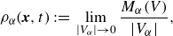
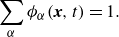
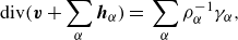
. We provide precise definitions of all quantities in the remainder of the article. A key property of the framework is its invariance to the set of fundamental variables, both before and after constitutive modelling (see figure 1).
$\sum _{\beta } \phi _{\beta } =1$
. We provide precise definitions of all quantities in the remainder of the article. A key property of the framework is its invariance to the set of fundamental variables, both before and after constitutive modelling (see figure 1).
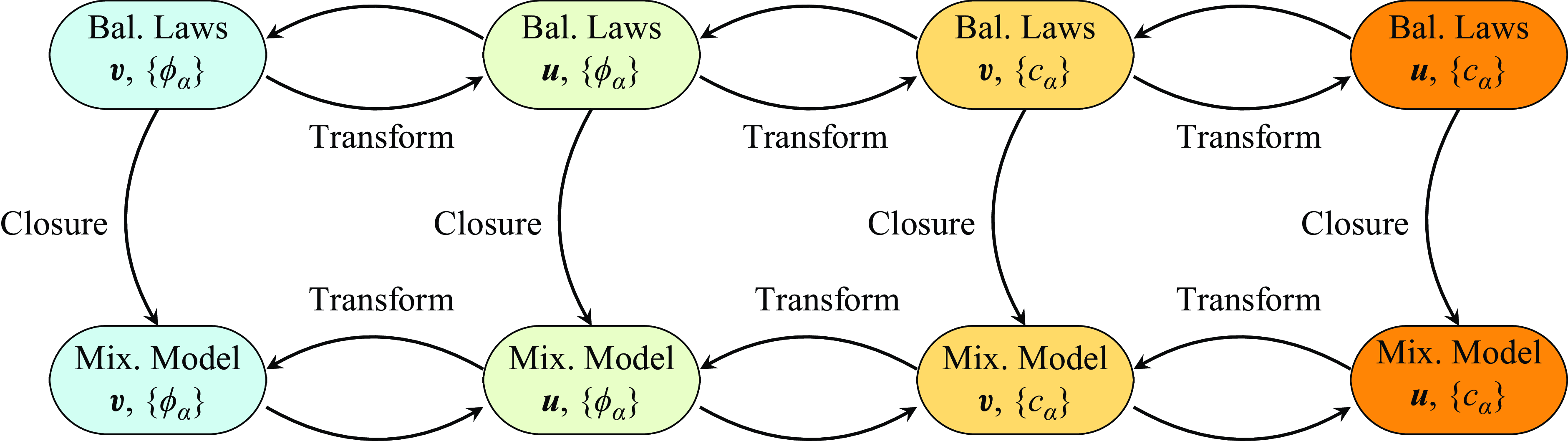
Figure 1. Invariance of the unified framework, both at the level of balance laws (Bal. Laws) and, after closure, at the level of mixture models (Mix. Model).
The classification as an NSCHAC model is evident in the combination of a momentum equation with ( $N$
) mass balance laws that are of Cahn–Hilliard Allen–Cahn type for specific free energy choices. The Cahn–Hilliard components appear in the third members of the mass balance laws, whereas the Allen–Cahn character materialises in the latter terms of the mass balance laws. Furthermore, the model – in both formulations – displays a strong coupling between the various equations, through the constituent densities
$N$
) mass balance laws that are of Cahn–Hilliard Allen–Cahn type for specific free energy choices. The Cahn–Hilliard components appear in the third members of the mass balance laws, whereas the Allen–Cahn character materialises in the latter terms of the mass balance laws. Furthermore, the model – in both formulations – displays a strong coupling between the various equations, through the constituent densities $\tilde {\rho }_\alpha$
, the velocity
$\tilde {\rho }_\alpha$
, the velocity $\boldsymbol{v}$
(or
$\boldsymbol{v}$
(or $\boldsymbol{u}$
) and the Lagrange multiplier pressure
$\boldsymbol{u}$
) and the Lagrange multiplier pressure $\lambda$
.
$\lambda$
.
The secondary objective of this article is to reveal connections between model (1.1) and (1.2) and existing models in the literature. First, we compare model (1.1)–(1.2) with the unified NSCHAC model (ten Eikelder et al. Reference ten Eikelder, van der Zee, Akkerman and Schillinger2023) for the situation of two phases. Subsequently, we compare the framework to that of Dong (Reference Dong2018). Finally, we discuss the connections of the proposed framework with the mixture-theory-compatible $N$
-phase model (ten Eikelder, van der Zee & Schillinger Reference ten Eikelder, van der Zee and Schillinger2024).
$N$
-phase model (ten Eikelder, van der Zee & Schillinger Reference ten Eikelder, van der Zee and Schillinger2024).
1.3. Plan of the paper
The remainder of the paper is organised as follows. In § 2 we present the continuum theory of rational mechanics for incompressible isothermal fluid mixtures, highlighting the connections between different quantities and formulations of evolution equations. Next, in § 3, we conduct constitutive modelling using the Coleman–Noll procedure. Following that, § 4 addresses the properties of the model. Subsequently, in § 5 we explore the connections of the properties of the model. Subsequently, in § 5, we explore the connections of the novel model with existing models in the literature. Finally, in § 6, we provide a conclusion and outlook.
2. Continuum mixture theory
The purpose of this section is to outline the continuum theory of mixtures for incompressible constituents, excluding thermal effects. This section aligns with ten Eikelder et al. (Reference ten Eikelder, van der Zee and Schillinger2024) at several points.
The continuum theory of mixtures is grounded in three general principles introduced in the pioneering work of Truesdell & Toupin (Reference Truesdell and Toupin1960):
-
(i) All properties of the mixture must be mathematical consequences of properties of the constituents.
-
(ii) So as to describe the motion of a constituent, we may in imagination isolate it from the rest of the mixture, provided we allow properly for the actions of the other constituents upon it.
-
(iii) The motion of the mixture is governed by the same equations as is a single body.
The first principle communicates that the mixture is made up of its constituent parts. The second principle asserts the connection of the different components of the physical model through interaction terms. Lastly, the latter principle states that one cannot distinguish the motion of a mixture from that of a single fluid.
In § 2.1 we introduce the fundamentals of the continuum theory of mixtures and the necessary kinematics. Then, in § 2.2 and § 2.3, we provide balance laws of individual constituents and associated mixtures.
2.1. Preliminaries
In the continuum theory of mixtures, the material body $\mathscr{B}$
comprises
$\mathscr{B}$
comprises $N$
constituent bodies
$N$
constituent bodies $\mathscr{B}_\alpha$
, with
$\mathscr{B}_\alpha$
, with $\alpha = 1, \dots , N$
. The bodies
$\alpha = 1, \dots , N$
. The bodies $\mathscr{B}_\alpha$
are permitted to simultaneously occupy a shared region in space. Denoting by
$\mathscr{B}_\alpha$
are permitted to simultaneously occupy a shared region in space. Denoting by $\boldsymbol{X}_{\alpha }$
the spatial position of a particle of
$\boldsymbol{X}_{\alpha }$
the spatial position of a particle of $\mathscr{B}_\alpha$
in the Lagrangian (reference) configuration, the (invertible) deformation map defines the spatial position of a particle:
$\mathscr{B}_\alpha$
in the Lagrangian (reference) configuration, the (invertible) deformation map defines the spatial position of a particle:
 \begin{align} \boldsymbol{x} := \boldsymbol{\chi }_{\alpha }(\boldsymbol{X}_{\alpha },t), \end{align}
where $\boldsymbol{x} \in \Omega$
, with
$\boldsymbol{x} \in \Omega$
, with $\Omega \in \mathbb{R}^d$
the domain (dimension
$\Omega \in \mathbb{R}^d$
the domain (dimension
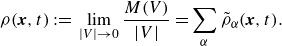
 $d$
). We refer for more details on continuum mixture theory to Truesdell & Toupin (Reference Truesdell and Toupin1960), and sketch the situation in figure 2.
$d$
). We refer for more details on continuum mixture theory to Truesdell & Toupin (Reference Truesdell and Toupin1960), and sketch the situation in figure 2.
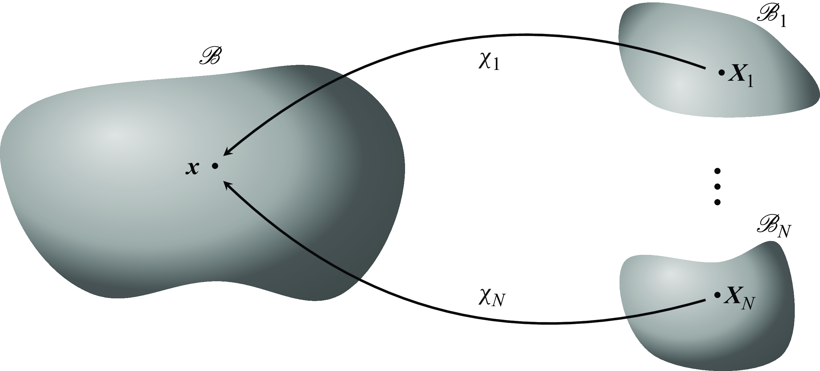
Figure 2. Situation sketch continuum mixture theory.
We introduce the constituent partial mass density $\tilde {\rho }_{\alpha }$
and specific mass density
$\tilde {\rho }_{\alpha }$
and specific mass density $\rho _{\alpha }\gt 0$
, respectively, as
$\rho _{\alpha }\gt 0$
, respectively, as
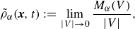 \begin{align} \tilde {\rho }_{\alpha }(\boldsymbol{x},t) :=&\, \displaystyle \lim _{ \vert V \vert \rightarrow 0} \frac {M_{\alpha }(V)}{\vert V \vert }, \end{align}
 \begin{align} \rho _{\alpha }(\boldsymbol{x},t) :=&\, \displaystyle \lim _{\vert V_{\alpha }\vert \rightarrow 0} \frac {M_{\alpha }(V)}{\vert V_{\alpha }\vert }, \end{align}
where $V \subset \Omega$
(measure
$V \subset \Omega$
(measure $\vert V \vert$
) is an arbitrary control volume around
$\vert V \vert$
) is an arbitrary control volume around $\boldsymbol{x}$
,
$\boldsymbol{x}$
, $V_{\alpha } \subset V$
(measure
$V_{\alpha } \subset V$
(measure $\vert V_{\alpha }\vert$
) is the volume of constituent
$\vert V_{\alpha }\vert$
) is the volume of constituent $\alpha$
so that
$\alpha$
so that $V =\cup _{\alpha }V_{\alpha }$
. Here, the constituents masses are
$V =\cup _{\alpha }V_{\alpha }$
. Here, the constituents masses are $M_{\alpha }=M_{\alpha }(V)$
, and the total mass in
$M_{\alpha }=M_{\alpha }(V)$
, and the total mass in $V$
is
$V$
is $M=M(V)=\sum _{\alpha }M_{\alpha }(V)$
. The mixture density is the sum of the partial mass densities:
$M=M(V)=\sum _{\alpha }M_{\alpha }(V)$
. The mixture density is the sum of the partial mass densities:
 \begin{align} \rho (\boldsymbol{x},t):=&\, \displaystyle \lim _{ \vert V \vert \rightarrow 0} \frac {M(V)}{\vert V \vert }=\displaystyle \sum _{\alpha }\tilde {\rho }_\alpha (\boldsymbol{x},t). \end{align}
Additionally, we introduce the mass concentrations (or mass fractions) and volume fractions, respectively, as:
 \begin{align} c_\alpha (\boldsymbol{x},t):=&\, \displaystyle \lim _{ \vert V \vert \rightarrow 0} \frac {M_{\alpha }(V)}{M(V)}=\frac {\tilde {\rho }_\alpha }{\rho }, \end{align}
 \begin{align} \phi _\alpha (\boldsymbol{x},t):=&\, \displaystyle \lim _{ \vert V \vert \rightarrow 0} \frac {|V_{\alpha }|}{|V|}=\frac {\tilde {\rho }_\alpha }{\rho _\alpha }, \end{align}
which sum up to one:
 \begin{align} \displaystyle \sum _{\alpha } c_{\alpha }(\boldsymbol{x},t)=&\, 1, \end{align}
 \begin{align} \displaystyle \sum _{\alpha } \phi _{\alpha }(\boldsymbol{x},t)=&\, 1. \end{align}
We assume that the constituents are incompressible, meaning that the specific mass densities are (constituent-wise) constant:
 \begin{align} \rho _\alpha (\boldsymbol{x},t) = \rho _\alpha . \end{align}
By means of the incompressibility of the constituents, (2.6), and the definitions (2.4), the volume fractions and concentrations are related by
 \begin{align} \phi _\alpha =&\, \frac {c_\alpha }{\rho _\alpha }\left (\sum _{\beta }\frac {c_{\beta }}{\rho _{\beta }}\right )^{-1}, \end{align}
 \begin{align} c_\alpha =&\, \rho _\alpha \phi _\alpha \left (\sum _{\beta }\rho _{\beta }\phi _{\beta }\right )^{-1}, \end{align}
for $\alpha =1, \ldots , N$
.
$\alpha =1, \ldots , N$
.
Remark 2.1 (Incompressibility $N$
-phase model). The relations (2.7) hinge on the assumption that the constituents are incompressible, i.e. definition (2.6), and the saturation constraint (2.5). The variables
$N$
-phase model). The relations (2.7) hinge on the assumption that the constituents are incompressible, i.e. definition (2.6), and the saturation constraint (2.5). The variables $\phi _\alpha$
(or
$\phi _\alpha$
(or $c_\alpha$
) are interdependent via (2.5), which must be considered explicitly when formulating or deducing relationships to avoid overdetermined or inconsistent expressions. For example, the mappings (2.7) are not invertible. We discuss these challenges throughout the article, and in Appendix B.
$c_\alpha$
) are interdependent via (2.5), which must be considered explicitly when formulating or deducing relationships to avoid overdetermined or inconsistent expressions. For example, the mappings (2.7) are not invertible. We discuss these challenges throughout the article, and in Appendix B.
Remark 2.2 (Alternative definitions incompressible mixtures). Besides the current definition of incompressible constituents (2.6), which is adopted frequently in the literature (see e.g. Li & Wang Reference Li and Wang2014, Dong Reference Dong2015, Reference Dong2018, Huang et al. Reference Huang, Lin and Ardekani2021), there exist other notions of incompressibility in mixture flows. We refer for an alternative to Bothe, Dreyer & Druet (Reference Bothe, Dreyer and Druet2023) and the references therein.
We proceed with the introduction of the material time derivative $\grave {\psi }_\alpha$
of the differentiable constituent function
$\grave {\psi }_\alpha$
of the differentiable constituent function $\psi _\alpha$
:
$\psi _\alpha$
:
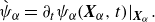 \begin{align} \grave {\psi }_\alpha =\partial _t\psi _{\alpha }(\boldsymbol{X}_{\alpha },t) \vert _{\boldsymbol{X}_\alpha }. \end{align}
Here we adopt the notation $\vert _{\boldsymbol{X}_\alpha }$
to indicate that
$\vert _{\boldsymbol{X}_\alpha }$
to indicate that $\boldsymbol{X}_\alpha$
is held fixed. The constituent velocity now follows as the constituent material derivative of the deformation map:
$\boldsymbol{X}_\alpha$
is held fixed. The constituent velocity now follows as the constituent material derivative of the deformation map:
 \begin{align} \boldsymbol{v}_{\alpha }(\boldsymbol{x},t)=\partial _t\boldsymbol{\chi }_{\alpha }(\boldsymbol{X}_{\alpha },t) \vert _{\boldsymbol{X}_\alpha } = \grave {\boldsymbol{\chi }}_\alpha . \end{align}
In contrast to the mixture density, there appear various mixture velocities in the literature. Among the most popular ones are the mass-averaged velocity, denoted $\boldsymbol{v}$
, and the volume-averaged velocity, denoted
$\boldsymbol{v}$
, and the volume-averaged velocity, denoted $\boldsymbol{u}$
, which are, respectively, given by
$\boldsymbol{u}$
, which are, respectively, given by
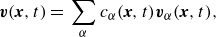 \begin{align} \boldsymbol{v}(\boldsymbol{x},t) =&\, \displaystyle \sum _{\alpha } c_\alpha (\boldsymbol{x},t) \boldsymbol{v}_\alpha (\boldsymbol{x},t), \end{align}
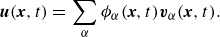 \begin{align} \boldsymbol{u}(\boldsymbol{x},t) =&\, \displaystyle \sum _{\alpha } \phi _\alpha (\boldsymbol{x},t) \boldsymbol{v}_\alpha (\boldsymbol{x},t). \end{align}
We introduce peculiar velocities of the constituents relative to both mixture velocities:
 \begin{align} \boldsymbol{w}_{\alpha }(\boldsymbol{x},t):=&\,\boldsymbol{v}_{\alpha }(\boldsymbol{x},t)-\boldsymbol{v}(\boldsymbol{x},t), \end{align}
 \begin{align} \boldsymbol{\omega }_{\alpha }(\boldsymbol{x},t):=&\,\boldsymbol{v}_{\alpha }(\boldsymbol{x},t)-\boldsymbol{u}(\boldsymbol{x},t). \end{align}
Additionally, we define the following (scaled) peculiar velocities (that depend on $\boldsymbol{x}$
and
$\boldsymbol{x}$
and $t$
):
$t$
):
 \begin{align} \boldsymbol{J}_\alpha :=&\, \tilde {\rho }_\alpha \boldsymbol{w}_\alpha , \end{align}
 \begin{align} \boldsymbol{h}_\alpha = &\, \phi _\alpha \boldsymbol{w}_\alpha , \end{align}
 \begin{align} \boldsymbol{J}_\alpha ^u = &\, \tilde {\rho }_\alpha \boldsymbol{\omega }_\alpha, \end{align}
 \begin{align} \boldsymbol{h}_\alpha ^u = &\, \phi _\alpha \boldsymbol{\omega }_\alpha . \end{align}
Remark 2.3 (Terminology peculiar velocities). The quantities (2.11) and (2.12) are in the literature often referred to as ‘diffusion velocities’ and ‘diffusive fluxes’, respectively. This terminology is natural because the terms (2.12) appear in constituent mass balance laws (see § 2.2) as flux terms, and their constitutive models (see § 3.4) have a diffusive character. However, utilising constitutive models for (2.12) is not essential (see ten Eikelder et al. Reference ten Eikelder, van der Zee and Schillinger2024), and therefore we use the terminology ‘(scaled) peculiar velocity’ to reflect their original definitions (2.11) and (2.12).
Direct consequences of (2.11), (2.12a ) and (2.12d ) are the following properties:
 \begin{align} \displaystyle \sum _{\alpha } \boldsymbol{J}_\alpha =&\, 0, \end{align}
 \begin{align} \displaystyle \sum _{\alpha } \boldsymbol{h}_\alpha ^u =&\, 0. \end{align}
The relation between the mass-averaged and volume-averaged velocities is specified in the following lemma.
Lemma 2.4 (Relation mass-averaged and volume-averaged velocities). The mass-averaged and volume-averaged velocity variables are related via
 \begin{align} \boldsymbol{u} =&\, \boldsymbol{v} + \displaystyle \sum _\alpha \rho _\alpha ^{-1} \boldsymbol{J}_\alpha = \boldsymbol{v} + \sum _\alpha \boldsymbol{h}_\alpha , \end{align}
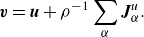 \begin{align} \boldsymbol{v} =&\, \boldsymbol{u} + \rho ^{-1} \sum _\alpha \boldsymbol{J}_\alpha ^u. \end{align}
Proof. These relations result from the following sequences of identities:
 \begin{align} \boldsymbol{u} &= \sum _\alpha \phi _\alpha \boldsymbol{v}_\alpha = \sum _\alpha \phi _\alpha \boldsymbol{w}_\alpha + \sum _\alpha \phi _\alpha \boldsymbol{v} = \sum _\alpha \rho _\alpha ^{-1} \boldsymbol{J}_\alpha + \boldsymbol{v}, \end{align}
 \begin{align} 0 &= \sum _\alpha \boldsymbol{J}_\alpha = \sum _\alpha \tilde {\rho }_\alpha (\boldsymbol{v}_\alpha -\boldsymbol{v}) = \sum _\alpha \tilde {\rho }_\alpha (\boldsymbol{v}_\alpha -\boldsymbol{u} + \boldsymbol{u}-\boldsymbol{v}) \nonumber \\ & = \sum _\alpha \boldsymbol{J}_\alpha ^u + \rho (\boldsymbol{u}-\boldsymbol{v}).\\ \nonumber \end{align}
The relation between the scaled peculiar velocities is displayed in the next lemma.
Lemma 2.5 (Relation scaled peculiar velocities). The scaled peculiar velocities are related via
 \begin{align} \boldsymbol{J}_\alpha =&\, \boldsymbol{J}_\alpha ^u - c_\alpha \sum _{\beta } \boldsymbol{J}_{\beta }^u, \end{align}
 \begin{align} \boldsymbol{J}_\alpha ^u =&\, \boldsymbol{J}_\alpha - \tilde {\rho }_\alpha \sum _{\beta } \rho _{\beta }^{-1} \boldsymbol{J}_{\beta }, \end{align}
 \begin{align} \boldsymbol{h}_\alpha =&\, \boldsymbol{h}_\alpha ^u - \phi _\alpha \rho ^{-1} \sum _{\beta } \rho _{\beta }\boldsymbol{h}_{\beta }^u, \end{align}
 \begin{align} \boldsymbol{h}_\alpha ^u =&\, \boldsymbol{h}_\alpha - \phi _\alpha \sum _{\beta } \boldsymbol{h}_{\beta }. \end{align}
Proof. These identities are a direct consequence of Lemma2.4.
Lastly, we define the material derivative of the mixture relative to the mass-averaged velocity:
 \begin{align} \dot {\psi }(\boldsymbol{x},t) =&\, \partial _t \psi (\boldsymbol{x},t) + \boldsymbol{v}(\boldsymbol{x},t)\ {\boldsymbol\cdot}\ \nabla \psi (\boldsymbol{x},t). \end{align}
2.2. Constituent balance laws
In the continuum theory of mixtures, each constituent moves according to a distinct set of balance laws, as specified by the second general principle. These laws incorporate terms that model the interactions among the different constituents. The following local balance laws apply to the motion of each constituent $\alpha = 1, \dots , N$
for all
$\alpha = 1, \dots , N$
for all $\boldsymbol{x}\in \Omega$
and
$\boldsymbol{x}\in \Omega$
and $t \gt 0$
:
$t \gt 0$
:
 \begin{align} \partial _t \tilde {\rho }_\alpha + \textrm{div}(\tilde {\rho }_\alpha \boldsymbol{v}_\alpha ) &=\, \gamma _\alpha , \end{align}
 \begin{align} \partial _t (\tilde {\rho }_\alpha \boldsymbol{v}_\alpha ) + \textrm{div} \left ( \tilde {\rho }_\alpha \boldsymbol{v}_\alpha \otimes \boldsymbol{v}_\alpha \right ) - \textrm{div} \boldsymbol{T}_\alpha - \tilde {\rho }_\alpha \boldsymbol{b}_\alpha &=\, \boldsymbol{\pi }_\alpha , \end{align}
 \begin{align} \boldsymbol{T}_\alpha -\boldsymbol{T}_\alpha ^{T} &=\,\boldsymbol{N}_\alpha . \end{align}
Equations (2.18a
) describe the local constituent mass balance laws, where the interaction terms $\gamma _{\alpha }$
denote the mass supply of constituent
$\gamma _{\alpha }$
denote the mass supply of constituent $\alpha$
due to chemical reactions with the other constituents. Then, (2.18b
) represent the local constituent linear momentum balance laws, where
$\alpha$
due to chemical reactions with the other constituents. Then, (2.18b
) represent the local constituent linear momentum balance laws, where $\boldsymbol{T}_\alpha$
is the Cauchy stress tensor of constituent
$\boldsymbol{T}_\alpha$
is the Cauchy stress tensor of constituent $\alpha$
,
$\alpha$
, $\boldsymbol{b}_\alpha$
is the constituent external body force, and
$\boldsymbol{b}_\alpha$
is the constituent external body force, and $\boldsymbol{\pi }_\alpha$
is the momentum exchange rate of constituent
$\boldsymbol{\pi }_\alpha$
is the momentum exchange rate of constituent $\alpha$
with the other constituents. We assume equal body forces (
$\alpha$
with the other constituents. We assume equal body forces ( $\boldsymbol{b}_\alpha = \boldsymbol{b}$
for
$\boldsymbol{b}_\alpha = \boldsymbol{b}$
for $\alpha = 1, \dots , N$
) throughout the article. Additionally, we restrict to gravitational body forces:
$\alpha = 1, \dots , N$
) throughout the article. Additionally, we restrict to gravitational body forces: $\boldsymbol{b} = -b \boldsymbol{\jmath } = -b \nabla y$
, with
$\boldsymbol{b} = -b \boldsymbol{\jmath } = -b \nabla y$
, with $y$
being the vertical coordinate,
$y$
being the vertical coordinate, $\boldsymbol{\jmath }$
the vertical unit vector, and
$\boldsymbol{\jmath }$
the vertical unit vector, and $b$
a constant. Finally, (2.18c
) describes the local constituent angular momentum balance with
$b$
a constant. Finally, (2.18c
) describes the local constituent angular momentum balance with $\boldsymbol{N}_\alpha$
the intrinsic moment of momentum.
$\boldsymbol{N}_\alpha$
the intrinsic moment of momentum.
We introduce a split of the mass transfer term into a conservative part and a potentially non-conservative contribution via
 \begin{align} \gamma _\alpha = \zeta _\alpha - \textrm{div} \boldsymbol{j}_\alpha . \end{align}
The mass balance laws (3.1a ) take the form
 \begin{align} \partial _t \tilde {\rho }_\alpha + \textrm{div}(\tilde {\rho }_\alpha \boldsymbol{v}_\alpha ) + \textrm{div} \boldsymbol{j}_\alpha = \zeta _\alpha . \end{align}
By invoking the definitions in § 2.1, one can deduce various alternative – equivalent – formulations of the constituent mass balance laws (2.18a ), such as
 \begin{align} \partial _t \tilde {\rho }_\alpha + \textrm{div}(\tilde {\rho }_\alpha \boldsymbol{v}) + \textrm{div} (\boldsymbol{J}_\alpha + \boldsymbol{j}_\alpha ) &=\, \zeta _\alpha , \end{align}
 \begin{align} \partial _t \tilde {\rho }_\alpha + \textrm{div}(\tilde {\rho }_\alpha \boldsymbol{u}) + \textrm{div} (\boldsymbol{J}_\alpha ^u + \boldsymbol{j}_\alpha ) &=\, \zeta _\alpha , \end{align}
 \begin{align} \partial _t \phi _\alpha + \textrm{div}(\phi _\alpha \boldsymbol{v}) + \textrm{div} \boldsymbol{h}_\alpha + \rho _\alpha ^{-1}\textrm{div} \boldsymbol{j}_\alpha &=\, \rho _\alpha ^{-1}\zeta _\alpha , \end{align}
 \begin{align} \partial _t \phi _\alpha + \textrm{div}\left (\phi _\alpha \boldsymbol{u}\right )+ \textrm{div}\boldsymbol{h}_\alpha ^u + \rho _\alpha ^{-1}\textrm{div} \boldsymbol{j}_\alpha &=\, \rho _\alpha ^{-1}\zeta _\alpha , \end{align}
 \begin{align} \rho \partial _t c_\alpha + \rho \boldsymbol{v} {\boldsymbol\cdot} \nabla c_\alpha + \textrm{div} (\boldsymbol{J}_\alpha + \boldsymbol{j}_\alpha ) &=\, \zeta _\alpha , \end{align}
 \begin{align} \rho \partial _t c_\alpha + \rho \boldsymbol{u} {\boldsymbol\cdot} \nabla c_\alpha + \textrm{div} (\boldsymbol{J}_\alpha ^u + \boldsymbol{j}_\alpha ) - c_\alpha \textrm{div}\!\left ( \sum _{\beta } \boldsymbol{J}_{\beta }^u \right ) &=\, \zeta _\alpha . \end{align}
Additionally, by invoking the relation (2.7) we can deduce numerous alternative – equivalent – formulations; for example, by inserting (2.7) into (2.21c ) we arrive at an uncommon formulation:
 \begin{align} \partial _t \left (\frac {c_\alpha }{\rho _\alpha }\left (\sum _{\beta }\frac {c_{\beta }}{\rho _{\beta }}\right )^{-1}\right ) + \textrm{ div}\left (\frac {c_\alpha }{\rho _\alpha }\left (\sum _{\beta }\frac {c_{\beta }}{\rho _{\beta }}\right )^{-1} \boldsymbol{v}\right ) &\nonumber \\ +\, \textrm{div} \boldsymbol{h}_\alpha + \rho _\alpha ^{-1}\textrm{div} \boldsymbol{j}_\alpha & = \rho _\alpha ^{-1}\zeta _\alpha . \end{align}
Similarly, one can write the constituent momentum balance laws (2.18b ) as
 \begin{align} \partial _t (\tilde {\rho }_\alpha \boldsymbol{v} + \boldsymbol{J}_\alpha ) + \textrm{div} \left ( \tilde {\rho }_\alpha \boldsymbol{v}\otimes \boldsymbol{v} +\boldsymbol{J}_\alpha \otimes \boldsymbol{v} + \boldsymbol{v}\otimes \boldsymbol{J}_\alpha \right )&\nonumber \\ - \, \textrm{div} \left (\boldsymbol{T}_\alpha - \tilde {\rho }_\alpha \boldsymbol{w}_\alpha \otimes \boldsymbol{w}_\alpha \right ) - \tilde {\rho }_\alpha \boldsymbol{b}_\alpha &=\, \boldsymbol{\pi }_\alpha , \end{align}
 \begin{align} \partial _t (\tilde {\rho }_\alpha \boldsymbol{u} + \boldsymbol{J}_\alpha ^u) + \textrm{div} \left ( \tilde {\rho }_\alpha \boldsymbol{u}\otimes \boldsymbol{u} +\boldsymbol{J}_\alpha ^u \otimes \boldsymbol{u} + \boldsymbol{u}\otimes \boldsymbol{J}_\alpha ^u \right )&\nonumber \\ + \, \textrm{div} \left (\tilde {\rho }_\alpha \boldsymbol{\omega }_\alpha \otimes \boldsymbol{\omega }_\alpha - \tilde {\rho }_\alpha \boldsymbol{w}_\alpha \otimes \boldsymbol{w}_\alpha \right )&\nonumber \\ -\, \textrm{div} \left (\boldsymbol{T}_\alpha - \tilde {\rho }_\alpha \boldsymbol{w}_\alpha \otimes \boldsymbol{w}_\alpha \right ) - \tilde {\rho }_\alpha \boldsymbol{b}_\alpha &=\, \boldsymbol{\pi }_\alpha . \end{align}
Finally, we introduce the constituent kinetic and gravitational energies, respectively, as
 \begin{align} \mathscr{K}_\alpha =&\,\tilde {\rho }_\alpha \|\boldsymbol{v}_\alpha \|^2/2, \end{align}
 \begin{align} \mathscr{G}_\alpha =&\,\tilde {\rho }_\alpha b y, \end{align}
where $\|\boldsymbol{v}_\alpha \|=(\boldsymbol{v}_\alpha\, {\boldsymbol\cdot}\, \boldsymbol{v}_\alpha )^{1/2}$
is the Euclidean norm of the velocity
$\|\boldsymbol{v}_\alpha \|=(\boldsymbol{v}_\alpha\, {\boldsymbol\cdot}\, \boldsymbol{v}_\alpha )^{1/2}$
is the Euclidean norm of the velocity $\boldsymbol{v}_\alpha$
.
$\boldsymbol{v}_\alpha$
.
2.3. Mixture balance laws
The standard formulation of mixture balance laws is well-known and follows from summing the balance laws (2.18) over all constituents. To establish the precise form, one can, for example, utilise the formulations (2.21a ) and (2.23a ) and invoke the identity (2.13a ) to obtain
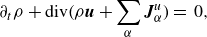
 \begin{align} \partial _t \rho + \textrm{div}(\rho \boldsymbol{v}) &=\, 0, \end{align}
 \begin{align} \partial _t (\rho \boldsymbol{v}) + \textrm{div} \left ( \rho \boldsymbol{v} \otimes \boldsymbol{v} \right ) - \textrm{div} \boldsymbol{T} - \rho \boldsymbol{b} &=\,0, \end{align}
 \begin{align} \boldsymbol{T}-\boldsymbol{T}^{T} &=\,0, \end{align}
where the mixture stress and mixture body force are given, respectively, by:
 \begin{align} \boldsymbol{T} =&\, \sum _\alpha \boldsymbol{T}_\alpha -\tilde {\rho }_\alpha \boldsymbol{w}_\alpha \otimes \boldsymbol{w}_\alpha , \end{align}
 \begin{align} \boldsymbol{b} =&\,\frac {1}{\rho }\sum _\alpha \tilde {\rho }_\alpha \boldsymbol{b}_\alpha , \end{align}
and where we have postulated the following balance conditions to hold as follows:
 \begin{align} \displaystyle \sum _\alpha \gamma _\alpha =&\, 0, \end{align}
 \begin{align} \displaystyle \sum _\alpha \boldsymbol{\pi }_\alpha =&\, 0, \end{align}
 \begin{align} \displaystyle \sum _\alpha \boldsymbol{N}_\alpha =&\, 0, \end{align}
and where we invoke (2.27a ) via
 \begin{align} \sum _\alpha \zeta _\alpha =&\, 0, \end{align}
 \begin{align} \sum _\alpha \boldsymbol{j}_\alpha =&\, 0. \end{align}
This formulation is compatible with the first general principle: the motion of the mixture is derived from the motion of its individual constituents. In addition, the postulate (2.27) is essential to ensure general principle three. Even though the forms presented in (2.21) and (2.23) are equivalent, the summation of these laws over the constituents does not provide a suitable system of mixture balance laws for each of the formulations. Namely, general principle three communicates that the resulting equations of the mixture are indistinguishable from that of a single body. Complying with this principle restricts the forms of the mass balance law to (2.21a
) and (2.21b
), and requires the identification of suitable mixture variables. These variables are $\rho$
,
$\rho$
, $\boldsymbol{v}$
,
$\boldsymbol{v}$
, $\boldsymbol{T}$
and
$\boldsymbol{T}$
and $\boldsymbol{b}$
, as defined earlier. In this sense, the framework of continuum mixture theory serves as a guideline for defining mixture variables. However, one can work with other variables as well; and this is fully compatible with the framework.
$\boldsymbol{b}$
, as defined earlier. In this sense, the framework of continuum mixture theory serves as a guideline for defining mixture variables. However, one can work with other variables as well; and this is fully compatible with the framework.
We discuss other formulations that emerge from (2.21) and (2.23). Summation of (2.21b )–(2.21f ) over the constituents provides
 \begin{align} \partial _t \rho + \textrm{div}\bigg(\rho \bigg(\boldsymbol{u} + \rho ^{-1}\sum _\alpha \boldsymbol{J}_\alpha ^u \bigg)\bigg) &=\, \sum _\alpha \gamma _\alpha = 0, \end{align}
 \begin{align} \textrm{div}\bigg(\boldsymbol{v} + \sum _\alpha \boldsymbol{h}_\alpha \bigg) &=\, \sum _\alpha \rho _\alpha ^{-1}\gamma _\alpha , \end{align}
 \begin{align} \textrm{div}\boldsymbol{u} &=\, \sum _\alpha \rho _\alpha ^{-1}\gamma _\alpha , \end{align}
 \begin{align} 0 &=\, \sum _\alpha \gamma _\alpha , \end{align}
where (2.29a
)–(2.29c
) follow from (2.21b
)–(2.21d
), respectively, and (2.29d
) results from both (2.21e
) and (2.21f
). We observe from (2.29a
) that the term in the inner brackets in the second term represents the mixture velocity. Obviously, this matches the mass-averaged velocity by invoking Lemma2.4. Next, note that (2.29b
) also follows from the summation over the constituents of (2.22). With the aid of Lemma2.4, one can infer that (2.29b
) and (2.29c
) are identical. Furthermore, $\boldsymbol{v} + \sum _\alpha \boldsymbol{h}_\alpha = \boldsymbol{u}$
is a divergence-free velocity whenever either (i) mass transfer is absent (
$\boldsymbol{v} + \sum _\alpha \boldsymbol{h}_\alpha = \boldsymbol{u}$
is a divergence-free velocity whenever either (i) mass transfer is absent ( $\gamma _\alpha = 0$
for all
$\gamma _\alpha = 0$
for all $\alpha$
), or (ii) the constituent densities match (
$\alpha$
), or (ii) the constituent densities match ( $\rho _\alpha = \rho _{\beta }$
for all
$\rho _\alpha = \rho _{\beta }$
for all $\alpha ,{\beta }$
). Next, (2.29d
) complies with the balance condition (2.27a
) and shows that no velocity divergence equation results from using concentration variables. Finally, the summation of (2.23) yields
$\alpha ,{\beta }$
). Next, (2.29d
) complies with the balance condition (2.27a
) and shows that no velocity divergence equation results from using concentration variables. Finally, the summation of (2.23) yields
 \begin{align} \partial _t \bigg(\rho \bigg(\boldsymbol{u} + \rho ^{-1}\sum _\alpha \boldsymbol{J}_\alpha ^u\bigg)\bigg) + \textrm{div} \bigg( \rho \bigg(\boldsymbol{u}\otimes \boldsymbol{u} + \rho ^{-1} \sum _\alpha \boldsymbol{J}_\alpha ^u \otimes \boldsymbol{u} + \rho ^{-1}\boldsymbol{u}\otimes \sum _\alpha \boldsymbol{J}_\alpha ^u \bigg)\bigg)\nonumber \\ + \, \textrm{div} \bigg( \sum _\alpha \tilde {\rho }_\alpha \boldsymbol{\omega }_\alpha \otimes \boldsymbol{\omega }_\alpha - \tilde {\rho }_\alpha \boldsymbol{w}_\alpha \otimes \boldsymbol{w}_\alpha \bigg)- \textrm{div} \boldsymbol{T} - \rho \boldsymbol{b} =\,0. \end{align}
Invoking Lemma2.4 and Lemma2.5, this may be written as
 \begin{align}& \partial _t \bigg(\rho \bigg(\boldsymbol{u} + \rho ^{-1}\sum _\alpha \boldsymbol{J}_\alpha ^u\bigg)\bigg) + \textrm{div} \bigg( \rho \bigg(\boldsymbol{u}\otimes \boldsymbol{u} + \rho ^{-1} \sum _\alpha \boldsymbol{J}_\alpha ^u \otimes \boldsymbol{u} + \rho ^{-1}\boldsymbol{u}\otimes \sum _\alpha \boldsymbol{J}_\alpha ^u \bigg)\bigg)\nonumber \\& \qquad + \, \textrm{div} \bigg( \rho ^{-1} \sum _\alpha \boldsymbol{J}_\alpha ^u\otimes \sum _\alpha \boldsymbol{J}_\alpha ^u\bigg) - \textrm{div} \boldsymbol{T} - \rho \boldsymbol{b} =\,0. \end{align}
One can infer equivalence with the mass-averaged momentum equation by noting the identities
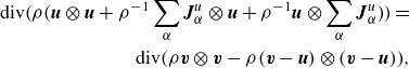 \begin{align} \textrm{div} \bigg ( \rho \bigg (\boldsymbol{u}\otimes \boldsymbol{u} + \rho ^{-1} \sum _\alpha \boldsymbol{J}_\alpha ^u \otimes \boldsymbol{u} + \rho ^{-1}\boldsymbol{u}\otimes \sum _\alpha \boldsymbol{J}_\alpha ^u \bigg )\bigg ) = \nonumber \\ \textrm{div} \bigg ( \rho \boldsymbol{v} \otimes \boldsymbol{v} -\rho (\boldsymbol{v}-\boldsymbol{u})\otimes (\boldsymbol{v}-\boldsymbol{u})\bigg ), \end{align}
 \begin{align} \textrm{div} \bigg ( \sum _\alpha \tilde {\rho }_\alpha \boldsymbol{\omega }_\alpha \otimes \boldsymbol{\omega }_\alpha - \tilde {\rho }_\alpha \boldsymbol{w}_\alpha \otimes \boldsymbol{w}_\alpha \bigg ) = \textrm{div} \bigg (\rho (\boldsymbol{v}-\boldsymbol{u})\otimes (\boldsymbol{v}-\boldsymbol{u})\bigg ). \end{align}
In summary, an – equivalent – formulation of mixture balance laws (2.25) in terms of the volume-averaged velocity is
 \begin{align} \partial _t \rho + \textrm{div}\bigg (\rho \boldsymbol{u} + \sum _\alpha \boldsymbol{J}_\alpha ^u \bigg ) &=\, 0, \end{align}
 \begin{align} \partial _t \bigg (\rho \boldsymbol{u} + \sum _\alpha \boldsymbol{J}_\alpha ^u\bigg ) + \textrm{div} \bigg ( \rho \boldsymbol{u}\otimes \boldsymbol{u} + \sum _\alpha \boldsymbol{J}_\alpha ^u \otimes \boldsymbol{u} \bigg .& \nonumber \\ + \bigg . \boldsymbol{u}\otimes \sum _\alpha \boldsymbol{J}_\alpha ^u + \rho ^{-1} \sum _\alpha \boldsymbol{J}_\alpha ^u\otimes \sum _\alpha \boldsymbol{J}_\alpha ^u\bigg ) - \textrm{div} \boldsymbol{T} - \rho \boldsymbol{b} &=\,0, \end{align}
 \begin{align} \boldsymbol{T}-\boldsymbol{T}^{T} &=\,0. \end{align}
The various forms presented in this section show that the set of balance laws, on both constituent level (§ 2.2) and mixture level (§ 2.3), is invariant to the set of fundamental variables.
We close this section with a remark on the kinetic and gravitational energies. According to the first metaphysical principle of mixture theory, the kinetic and gravitational energies of the mixture equal the summation of the constituent energies:
 \begin{align} \mathscr{K} =&\, \displaystyle \sum _{\alpha } \mathscr{K}_\alpha , \end{align}
 \begin{align} \mathscr{G} =&\, \displaystyle \sum _{\alpha } \mathscr{G}_\alpha . \end{align}
The kinetic energy of the mixture can be decomposed as
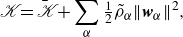 \begin{align} \mathscr{K} =&\, \bar {\mathscr{K}} + \displaystyle \sum _{\alpha } \tfrac {1}{2} \tilde {\rho }_\alpha \|\boldsymbol{w}_\alpha \|^2, \end{align}
 \begin{align} \bar {\mathscr{K}} =&\, \tfrac {1}{2} \rho \|\boldsymbol{v}\|^2, \end{align}
where $\bar {\mathscr{K}}$
represents the kinetic energy of the mixture variables, and where the other term is the kinetic energy of the constituents utilising the peculiar velocity. The second terms may also be expressed in terms of volume-averaged quantities:
$\bar {\mathscr{K}}$
represents the kinetic energy of the mixture variables, and where the other term is the kinetic energy of the constituents utilising the peculiar velocity. The second terms may also be expressed in terms of volume-averaged quantities:
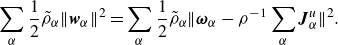 \begin{align} \displaystyle \sum _{\alpha } \frac {1}{2} \tilde {\rho }_\alpha \|\boldsymbol{w}_\alpha \|^2 = \displaystyle \sum _{\alpha } \frac {1}{2} \tilde {\rho }_\alpha \Bigg\|\boldsymbol{\omega }_\alpha - \rho ^{-1} \sum _\alpha \boldsymbol{J}_\alpha ^u \Bigg\|^2. \end{align}
3. Constitutive modelling
This section details the development of constitutive models under the constraints of an energy-dissipative postulate. First, § 3.1 outlines the fundamental assumptions and modelling choices. Next, § 3.2 establishes the constitutive modelling restriction introduced in § 3.1, and § 3.3 describes alternative modelling classes. Finally, in § 3.4, we select particular constitutive models that adhere to these established restrictions.
3.1. Assumptions and modelling choices
Rather than using the complete set of balance laws as given in (2.18a ), (2.18b ) and (2.18c ), we limit our focus to the simplified subset:
 \begin{align} \partial _t \phi _\alpha + \textrm{div}(\phi _\alpha \boldsymbol{v}) + \rho _\alpha ^{-1}\textrm{div} \boldsymbol{H}_\alpha &=\, \rho _\alpha ^{-1}\zeta _\alpha , \end{align}
 \begin{align} \partial _t (\rho \boldsymbol{v}) + \textrm{div} \left ( \rho \boldsymbol{v}\otimes \boldsymbol{v} \right ) - \textrm{div} \boldsymbol{T} - \rho \boldsymbol{b} &=\,0, \end{align}
 \begin{align} \boldsymbol{T}-\boldsymbol{T}^{T} &=\,0, \end{align}
with $\boldsymbol{H}_\alpha := \boldsymbol{J}_\alpha + \boldsymbol{j}_\alpha$
, where (3.1a
) holds for constituents
$\boldsymbol{H}_\alpha := \boldsymbol{J}_\alpha + \boldsymbol{j}_\alpha$
, where (3.1a
) holds for constituents $\alpha =1,\ldots ,N$
. At this point, the system comprises the unknown quantities: volume fractions
$\alpha =1,\ldots ,N$
. At this point, the system comprises the unknown quantities: volume fractions $\phi _\alpha$
(
$\phi _\alpha$
( $\alpha = 1,\ldots ,N$
), where we recall the identity (2.4b
), mass-averaged mixture velocity
$\alpha = 1,\ldots ,N$
), where we recall the identity (2.4b
), mass-averaged mixture velocity $\boldsymbol{v}$
, peculiar velocities
$\boldsymbol{v}$
, peculiar velocities $\boldsymbol{J}_\alpha$
(
$\boldsymbol{J}_\alpha$
( $\alpha = 1,\ldots ,N$
), mass transfer terms
$\alpha = 1,\ldots ,N$
), mass transfer terms $\zeta _\alpha , \boldsymbol{j}_\alpha$
(
$\zeta _\alpha , \boldsymbol{j}_\alpha$
( $\alpha = 1,\ldots ,N$
) and mixture stress
$\alpha = 1,\ldots ,N$
) and mixture stress $\boldsymbol{T}$
. In order to close the system, we seek for constitutive models for
$\boldsymbol{T}$
. In order to close the system, we seek for constitutive models for $\boldsymbol{J}_\alpha$
,
$\boldsymbol{J}_\alpha$
, $\boldsymbol{j}_\alpha$
,
$\boldsymbol{j}_\alpha$
, $\zeta _\alpha$
and
$\zeta _\alpha$
and $\boldsymbol{T}$
. Seeking for constitutive models for the peculiar velocities
$\boldsymbol{T}$
. Seeking for constitutive models for the peculiar velocities $\boldsymbol{J}_\alpha$
could be perceived as a simplification procedure. Namely, substituting a constitutive model (in § 3.4), in general, violates the continuum mixture theory definitions (2.12). We discard these definitions (2.12) in the following, but design models compatible with Lemma2.4 and Lemma2.5 to ensure invariance with respect to the set of fundamental variables. Instead of working with
$\boldsymbol{J}_\alpha$
could be perceived as a simplification procedure. Namely, substituting a constitutive model (in § 3.4), in general, violates the continuum mixture theory definitions (2.12). We discard these definitions (2.12) in the following, but design models compatible with Lemma2.4 and Lemma2.5 to ensure invariance with respect to the set of fundamental variables. Instead of working with $N$
velocities quantities
$N$
velocities quantities $\boldsymbol{v}_\alpha$
, the simplified system contains a single unknown velocity quantity
$\boldsymbol{v}_\alpha$
, the simplified system contains a single unknown velocity quantity $\boldsymbol{v}$
and constitutive models for peculiar velocities
$\boldsymbol{v}$
and constitutive models for peculiar velocities $\boldsymbol{J}_\alpha$
. This is compatible with the structure of the system: the full system is composed of
$\boldsymbol{J}_\alpha$
. This is compatible with the structure of the system: the full system is composed of $N$
linear momentum (mixture) balance laws whereas the simplified system contains a single linear momentum balance law. Additionally, we enforce the balance condition for the peculiar velocities (2.13a
) and the mass transfer terms (2.27a
) as follows:
$N$
linear momentum (mixture) balance laws whereas the simplified system contains a single linear momentum balance law. Additionally, we enforce the balance condition for the peculiar velocities (2.13a
) and the mass transfer terms (2.27a
) as follows:
 \begin{align} \sum _\alpha \boldsymbol{J}_\alpha =&\, 0, \end{align}
 \begin{align} \sum _\alpha \boldsymbol{j}_\alpha =&\, 0, \end{align}
 \begin{align} \sum _\alpha \zeta _\alpha =&\, 0, \end{align}
where we recall the decomposition (2.19). The system (3.1) contains the unknown variables $\boldsymbol{v}$
and
$\boldsymbol{v}$
and $\phi _\alpha$
(
$\phi _\alpha$
( $\alpha = 1,\ldots ,N$
). We emphasise that directly enforcing the summation condition (2.5b
) at this point would imply that the set
$\alpha = 1,\ldots ,N$
). We emphasise that directly enforcing the summation condition (2.5b
) at this point would imply that the set $\left \{\phi _\alpha \right \}_{\alpha =1,\ldots ,N}$
comprises
$\left \{\phi _\alpha \right \}_{\alpha =1,\ldots ,N}$
comprises $N-1$
independent variables. As such, system (3.1) would have a degenerate nature; it contains
$N-1$
independent variables. As such, system (3.1) would have a degenerate nature; it contains $N+1$
equations for
$N+1$
equations for $N$
variables (we preclude (2.25c
) in this count). Instead, a natural approach to restore the balance is by enforcing the constraint with a Lagrange multiplier construction, see § 3.2.
$N$
variables (we preclude (2.25c
) in this count). Instead, a natural approach to restore the balance is by enforcing the constraint with a Lagrange multiplier construction, see § 3.2.
Remark 3.1 (Classification). The previous assumptions lead to a model that includes $N$
constituent mass balance laws along with a single momentum balance law. According to the classification by Hutter & Jöhnk (Reference Hutter and Jöhnk2013), this configuration aligns best with a class-I model.
$N$
constituent mass balance laws along with a single momentum balance law. According to the classification by Hutter & Jöhnk (Reference Hutter and Jöhnk2013), this configuration aligns best with a class-I model.
We adopt the well-known Coleman–Noll procedure (Coleman & Noll Reference Coleman and Noll1974) as a guiding principle to design constitutive models. For this purpose, we postulate the energy-dissipation law:
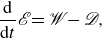 \begin{align} \frac {\textrm{d}}{\textrm{d}t} \mathscr{E} = \mathscr{W} - \mathscr{D}, \end{align}
satisfying $\mathscr{D}\geqslant 0$
. The total energy comprises the Helmholtz free energy, the kinetic energy and the gravitational energy:
$\mathscr{D}\geqslant 0$
. The total energy comprises the Helmholtz free energy, the kinetic energy and the gravitational energy:
 \begin{align} \mathscr{E} = \displaystyle \int _{\mathcal{R}(t)}(\Psi + \bar {\mathscr{K}} + \mathscr{G})\,\textrm{d}v. \end{align}
In this context, $\mathcal{R}=\mathcal{R}(t) \subset \Omega$
refers to a time-dependent control volume with volume element
$\mathcal{R}=\mathcal{R}(t) \subset \Omega$
refers to a time-dependent control volume with volume element $\textrm{d}v$
and a unit outward normal
$\textrm{d}v$
and a unit outward normal $\boldsymbol{\nu }$
that is transported by the velocity field
$\boldsymbol{\nu }$
that is transported by the velocity field $\boldsymbol{v}$
. Additionally,
$\boldsymbol{v}$
. Additionally, $\mathscr{W}$
represents a work rate term on the boundary
$\mathscr{W}$
represents a work rate term on the boundary $\partial \mathcal{R}(t)$
(with boundary element
$\partial \mathcal{R}(t)$
(with boundary element $\textrm{d}a$
), and
$\textrm{d}a$
), and $\mathscr{D}$
denotes the dissipation within the interior of
$\mathscr{D}$
denotes the dissipation within the interior of $\mathcal{R}(t)$
.
$\mathcal{R}(t)$
.
Remark 3.2 (Energy-dissipation postulate). As mentioned in ten Eikelder et al. (Reference ten Eikelder, van der Zee, Akkerman and Schillinger2023, Reference ten Eikelder, van der Zee and Schillinger2024), the energy-dissipation statement (3.3) can be perceived as an approximation of the second law of thermodynamics for mixtures.
We postulate that the free energy to pertain to the constitutive class is:
 \begin{align} \Psi =&\, \hat {\Psi }\left (\left \{\phi _\alpha \right \}_{\alpha =1,\ldots ,N},\left \{\nabla \phi _\alpha \right \}_{\alpha =1,\ldots ,N}\right ), \end{align}
and introduce the chemical potential quantities ( $\alpha = 1,\ldots ,N$
)
$\alpha = 1,\ldots ,N$
)
 \begin{align} \hat {\mu }_\alpha =&\, \frac { \partial \hat {\Psi }}{\partial \phi _\alpha } - \textrm{div}\frac {\partial \hat {\Psi }}{\partial \nabla \phi _\alpha }. \end{align}
At this point the volume fractions $\left \{\phi _\alpha \right \}_{\alpha =1,\ldots ,N}$
(and their gradients
$\left \{\phi _\alpha \right \}_{\alpha =1,\ldots ,N}$
(and their gradients $\left \{\nabla \phi _\alpha \right \}_{\alpha =1,\ldots ,N}$
) are independent quantities and (3.5) and (3.6) are obviously well-defined. However, this is no longer the case when the saturation constraint (2.5b
) would be directly enforced, which would make the chemical potentials individually arbitrary. Namely, addition of the term
$\left \{\nabla \phi _\alpha \right \}_{\alpha =1,\ldots ,N}$
) are independent quantities and (3.5) and (3.6) are obviously well-defined. However, this is no longer the case when the saturation constraint (2.5b
) would be directly enforced, which would make the chemical potentials individually arbitrary. Namely, addition of the term $(1-\sum _\alpha \phi _\alpha )$
to
$(1-\sum _\alpha \phi _\alpha )$
to $\hat {\Psi }$
does not alter it, but it modifies the chemical potentials
$\hat {\Psi }$
does not alter it, but it modifies the chemical potentials $\mu _\alpha$
. We return to this point at the end of this subsection.
$\mu _\alpha$
. We return to this point at the end of this subsection.
Remark 3.3 (Reduced free energy class). Instead of utilising the class (3.5), one can also directly enforce the summation constraint (2.5b) to arrive at a class with reduced dependency. In general, this breaks the symmetry of the approach, and therefore we do not adopt this alternative here. We discuss this option in Appendix A.
Remark 3.4 (Concentration-dependent free energy class). One can also work with a constituent class that depends on concentration quantities. We discuss this option in § 3.3.
3.2. Modelling restriction
Moving forward, we study in detail the restriction (3.3). First, we analyse the evolution of the energy (3.4). Through the application of the Reynolds transport theorem to the free energy $\hat {\Psi }$
, we have
$\hat {\Psi }$
, we have
 \begin{align} \frac {\textrm{d}}{\textrm{d}t}\displaystyle \int _{\mathcal{R}(t)} \hat {\Psi } \,\textrm{d}v = \displaystyle \int _{\mathcal{R}(t)} \partial _t \hat {\Psi } \,\textrm{d}v + \displaystyle \int _{\partial \mathcal{R}(t)} \hat {\Psi } \boldsymbol{v} {\boldsymbol\cdot} \boldsymbol{\nu } \,\textrm{d}a. \end{align}
We notice that directly enforcing the summation constraint (2.5b ) would not alter the derivative of the free energy class (3.5).
Lemma 3.5 (Derivative of the free energy). The derivative of the free energy class (3.5) , i.e.
 \begin{align} \textrm{d}\hat {\Psi } = \sum _{\alpha } \frac {\partial \hat {\Psi }}{\partial \phi _\alpha } \textrm{d}\phi _\alpha + \sum _{\alpha } \frac {\partial \hat {\Psi }}{\partial \nabla \phi _\alpha } \textrm{d}(\nabla \phi _\alpha ), \end{align}
is not altered by enforcing the summation constraint (2.5b), where $\textrm{d}$
is the derivative operator.
$\textrm{d}$
is the derivative operator.
Proof. See LemmaA.2.
Invoking Lemma3.5 and the divergence theorem yields
 \begin{align} \frac {\textrm{d}}{\textrm{d}t}\int _{\mathcal{R}(t)} \hat {\Psi } \,\textrm{d}v = \int _{\mathcal{R}(t)} &\ \hat {\Psi } \,\textrm{div} \boldsymbol{v} + \sum _{\alpha }\frac {\partial \hat {\Psi }}{\partial \phi _\alpha } \dot {\phi }_\alpha +\sum _{\alpha } \frac {\partial \hat {\Psi }}{\partial \nabla \phi _\alpha }{\boldsymbol{\cdot}} \left (\nabla \phi _\alpha \right )^{\boldsymbol{\cdot}}\,\textrm{d}v. \end{align}
Integrating by parts provides
 \begin{align} \frac {\textrm{d}}{\textrm{d}t}\displaystyle \int _{\mathcal{R}(t)} \hat {\Psi } \,\textrm{d}v =&\, \displaystyle \int _{\mathcal{R}(t)} \hat {\Psi }\,\textrm{div} \boldsymbol{v} + \sum _{\alpha } \hat {\mu }_\alpha \dot {\phi }_\alpha - \sum _{\alpha } \nabla \phi _\alpha \otimes \frac {\partial \hat {\Psi }}{\partial \nabla \phi _\alpha }: \nabla \boldsymbol{v} \,\textrm{d}v \nonumber \\ &\,+ \displaystyle \int _{\partial \mathcal{R}(t)}\sum _{\alpha } \dot {\phi }_\alpha \frac {\partial \hat {\Psi }}{\partial \nabla \phi _\alpha }{\boldsymbol\cdot} \boldsymbol{\nu } \,\textrm{d}a, \end{align}
where we have substituted the identity
 \begin{align} (\nabla \unicode{x03C8} )^{\boldsymbol{\cdot}} = \nabla (\dot {\psi }) - (\nabla \psi )^{T}\nabla \boldsymbol{v} \end{align}
for $\psi = \phi _\alpha$
. We note that the free energy terms are well-defined.
$\psi = \phi _\alpha$
. We note that the free energy terms are well-defined.
Lemma 3.6 (Well-defined free energy terms). The following free energy terms in(3.10)are well-defined when enforcing the summation constraint (2.5b):
 \begin{align} \sum _{\alpha } \hat {\mu }_\alpha \dot {\phi }_\alpha ; \quad \sum _{\alpha } \nabla \phi _\alpha \otimes \frac {\partial \hat {\Psi }}{\partial \nabla \phi _\alpha }; \quad \sum _{\alpha } \dot {\phi }_\alpha \frac {\partial \hat {\Psi }}{\partial \nabla \phi _\alpha }. \end{align}
Proof. See LemmaA.3.
Substituting the constituent mass balance laws (3.1a ) provides
 \begin{align} \frac {\textrm{d}}{\textrm{d}t}\displaystyle \int _{\mathcal{R}(t)} \hat {\Psi } \,\textrm{d}v =&\, \displaystyle \int _{\mathcal{R}(t)} \hat {\Psi }\,\textrm{div} \boldsymbol{v} + \sum _{\alpha } \hat {\mu }_\alpha \left(-\phi _\alpha \textrm{ div}\boldsymbol{v} - \rho _\alpha ^{-1}\textrm{div} \boldsymbol{H}_\alpha + \rho _\alpha ^{-1}\zeta _\alpha \right) \nonumber \\ &- \sum _{\alpha } \nabla \phi _\alpha \otimes \frac {\partial \hat {\Psi }}{\partial \nabla \phi _\alpha }: \nabla \boldsymbol{v} \,\textrm{d}v + \displaystyle \int _{\partial \mathcal{R}(t)}\sum _{\alpha } \dot {\phi }_\alpha \frac {\partial \hat {\Psi }}{\partial \nabla \phi _\alpha }{\boldsymbol\cdot} \boldsymbol{\nu } \,\textrm{d}a, \end{align}
where we recall $\boldsymbol{H}_\alpha = \boldsymbol{J}_\alpha + \boldsymbol{j}_\alpha$
. By again applying integration by parts one can infer that
$\boldsymbol{H}_\alpha = \boldsymbol{J}_\alpha + \boldsymbol{j}_\alpha$
. By again applying integration by parts one can infer that
 \begin{align} \frac {\textrm{d}}{\textrm{d}t}\displaystyle \int _{\mathcal{R}(t)} \sum _{\alpha } \hat {\Psi } \,\textrm{d}v = &\, \displaystyle \int _{\mathcal{R}(t)} \hat {\Psi }\,\textrm{div} \boldsymbol{v} -\sum _{\alpha } \hat {\mu }_\alpha \phi _\alpha \textrm{div}\boldsymbol{v} + \sum _{\alpha } \nabla (\rho _\alpha ^{-1}\hat {\mu }_\alpha )\ {\boldsymbol\cdot}\ \boldsymbol{H}_\alpha \nonumber \\ &\ \ \ - \sum _{\alpha } \nabla \phi _\alpha \otimes \frac {\partial \hat {\Psi }}{\partial \nabla \phi _\alpha }: \nabla \boldsymbol{v} + \sum _{\alpha } \rho _\alpha ^{-1}\hat {\mu }_\alpha \zeta _\alpha \,\textrm{d}v\nonumber \\ &\,+ \displaystyle \int _{\partial \mathcal{R}(t)}\sum _{\alpha } \left (\dot {\phi }_\alpha \frac {\partial \hat {\Psi }}{\partial \nabla \phi _\alpha }-\rho _\alpha ^{-1}\hat {\mu }_\alpha \boldsymbol{H}_\alpha \right )\,{\boldsymbol\cdot}\, \boldsymbol{\nu } \,\textrm{d}a. \end{align}
Next, the evolution of the kinetic and gravitational energies take the form (see ten Eikelder et al. (Reference ten Eikelder, van der Zee, Akkerman and Schillinger2023) for details)
 \begin{align} \frac {\textrm{d}}{\textrm{d}t}\displaystyle \int _{\mathcal{R}(t)} \mathscr{K} \,\textrm{d}v =&\, \displaystyle \int _{\mathcal{R}(t)} - \nabla \boldsymbol{v} : \boldsymbol{T}+\rho \boldsymbol{v}\ {\boldsymbol\cdot}\ \boldsymbol{b} \,\textrm{d}v+ \displaystyle \int _{\partial \mathcal{R}(t)} \boldsymbol{v}\ {\boldsymbol\cdot}\ \boldsymbol{T} \boldsymbol{\nu } \,\textrm{d}a, \end{align}
 \begin{align} \frac {\textrm{d}}{\textrm{d}t}\displaystyle \int _{\mathcal{R}(t)} \mathscr{G} \,\textrm{d}v =&\,- \displaystyle \int _{\mathcal{R}(t)} \rho \boldsymbol{v}\ {\boldsymbol\cdot}\ \boldsymbol{b}\,\textrm{d}v. \end{align}
The superposition of (3.14) and (3.15) provides the evolution of the total energy:
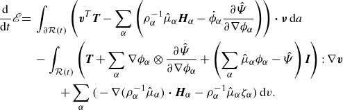 \begin{align} \frac {\textrm{d}}{\textrm{d}t} \mathscr{E} = &\, \displaystyle \int _{\partial \mathcal{R}(t)}\left (\boldsymbol{v}^{T}\boldsymbol{T}-\sum _{\alpha } \left (\rho _\alpha ^{-1}\hat {\mu }_\alpha \boldsymbol{H}_\alpha -\dot {\phi }_\alpha \frac {\partial \hat {\Psi }}{\partial \nabla \phi _\alpha }\right )\right ){\boldsymbol\cdot}\, \boldsymbol{\nu } \,\textrm{d}a \nonumber \\ &\,- \displaystyle \int _{\mathcal{R}(t)} \left (\boldsymbol{T} +\sum _{\alpha } \nabla \phi _\alpha \otimes \frac {\partial \hat {\Psi }}{\partial \nabla \phi _\alpha } +\left (\sum _{\alpha } \hat {\mu }_\alpha \phi _\alpha - \hat {\Psi }\right )\boldsymbol{I}\right ):\nabla \boldsymbol{v}\nonumber \\ &\,\,\,\,\,\,\,\,\,\,\,+ \sum _{\alpha }\Big(-\nabla \big(\rho _\alpha ^{-1}\hat {\mu }_\alpha \big)\ {\boldsymbol\cdot}\ \boldsymbol{H}_\alpha - \rho _\alpha ^{-1}\hat {\mu }_\alpha \zeta _\alpha \Big)\,\textrm{d}v. \end{align}
As mentioned in § 3.1, the system of balance laws (3.1) subjected to the balance conditions (3.2) is degenerate. Namely, the terms $\nabla \boldsymbol{v}$
,
$\nabla \boldsymbol{v}$
, $\boldsymbol{H}_\alpha$
and
$\boldsymbol{H}_\alpha$
and $\zeta _\alpha$
are connected via (2.29b
). This manifests itself in the energy dissipation statement (3.16). The degeneracy needs to be eliminated in order to exploit the energy-dissipation condition as a guiding principle for constitutive modelling. To this purpose we enforce (2.29b
) with the Lagrange multiplier construction:
$\zeta _\alpha$
are connected via (2.29b
). This manifests itself in the energy dissipation statement (3.16). The degeneracy needs to be eliminated in order to exploit the energy-dissipation condition as a guiding principle for constitutive modelling. To this purpose we enforce (2.29b
) with the Lagrange multiplier construction:
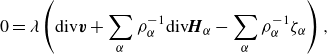 \begin{align} 0=&\, \lambda \left ( \textrm{div}\boldsymbol{v} + \displaystyle \sum _{\alpha } \rho _\alpha ^{-1} \textrm{div} \boldsymbol{H}_\alpha - \displaystyle \sum _{\alpha }\rho _\alpha ^{-1}\zeta _\alpha \right ), \end{align}
where $\lambda$
is the scalar Lagrange multiplier.
$\lambda$
is the scalar Lagrange multiplier.
Remark 3.7 (Lagrange multiplier constraint). Recalling Lemma 2.4, we observe that the Lagrange multiplier $\lambda$
enforces the constraint (2.29c). As such, in absence of mass transfer (
$\lambda$
enforces the constraint (2.29c). As such, in absence of mass transfer ( $\gamma _\alpha =0$
,
$\gamma _\alpha =0$
, $\alpha =1,\ldots ,N$
), it constrains
$\alpha =1,\ldots ,N$
), it constrains $\textrm{div}\boldsymbol{u}=0$
.
$\textrm{div}\boldsymbol{u}=0$
.
Integrating (3.17) over $\mathcal{R}(t)$
and subtracting the result from (3.16) provides
$\mathcal{R}(t)$
and subtracting the result from (3.16) provides
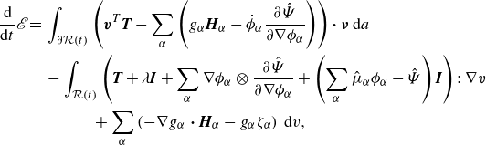 \begin{align} \frac {\textrm{d}}{\textrm{d}t} \mathscr{E} = &\, \displaystyle \int _{\partial \mathcal{R}(t)}\left (\boldsymbol{v}^{T}\boldsymbol{T}-\sum _{\alpha } \left (g_\alpha \boldsymbol{H}_\alpha -\dot {\phi }_\alpha \frac {\partial \hat {\Psi }}{\partial \nabla \phi _\alpha }\right )\right ){\boldsymbol\cdot}\, \boldsymbol{\nu } \,\textrm{d}a \nonumber \\ &\,- \displaystyle \int _{\mathcal{R}(t)} \left (\boldsymbol{T} + \lambda \boldsymbol{I} +\sum _{\alpha } \nabla \phi _\alpha \otimes \frac {\partial \hat {\Psi }}{\partial \nabla \phi _\alpha } +\left (\sum _{\alpha } \hat {\mu }_\alpha \phi _\alpha - \hat {\Psi }\right )\boldsymbol{I}\right ):\nabla \boldsymbol{v}\nonumber \\ &\,\,\,\,\,\,\,\,\,\,\,\,\,\,\,\,+ \sum _{\alpha }\left (-\nabla g_\alpha\ {\boldsymbol\cdot}\ \boldsymbol{H}_\alpha - g_\alpha \zeta _\alpha \right )\,\textrm{d}v, \end{align}
where we have utilised Gauß divergence theorem, and where we have defined the (generalised) chemical potential quantities:
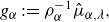 \begin{align} g_\alpha :=&\, \rho _\alpha ^{-1}\hat {\mu }_{\alpha ,\lambda }, \end{align}
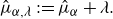 \begin{align} \hat {\mu }_{\alpha ,\lambda } :=&\, \hat {\mu }_\alpha +\lambda . \end{align}
We identify the rate of work and the dissipation, respectively, as
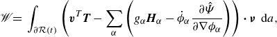 \begin{align} \mathscr{W} =&\, \displaystyle \int _{\partial \mathcal{R}(t)}\left (\boldsymbol{v}^{T}\boldsymbol{T}-\sum _{\alpha } \left (g_\alpha \boldsymbol{H}_\alpha -\dot {\phi }_\alpha \frac {\partial \hat {\Psi }}{\partial \nabla \phi _\alpha }\right )\right ){\boldsymbol\cdot}\, \boldsymbol{\nu } \,\textrm{ d}a, \end{align}
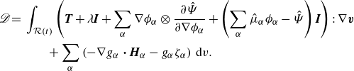 \begin{align} \mathscr{D} =&\,\displaystyle \int _{\mathcal{R}(t)} \left (\boldsymbol{T} + \lambda \boldsymbol{I} +\sum _{\alpha } \nabla \phi _\alpha \otimes \frac {\partial \hat {\Psi }}{\partial \nabla \phi _\alpha } +\left (\sum _{\alpha } \hat {\mu }_\alpha \phi _\alpha - \hat {\Psi }\right )\boldsymbol{I}\right ):\nabla \boldsymbol{v}\nonumber \\ &\qquad + \sum _{\alpha }\left (-\nabla g_\alpha\ {\boldsymbol\cdot}\ \boldsymbol{H}_\alpha -g_\alpha \zeta _\alpha \right )\,\textrm{d}v. \end{align}
Given the arbitrary nature of the control volume $\mathcal{R}=\mathcal{R}(t)$
, the fulfilment of the energy-dissipation law is contingent upon satisfying the local inequality:
$\mathcal{R}=\mathcal{R}(t)$
, the fulfilment of the energy-dissipation law is contingent upon satisfying the local inequality:
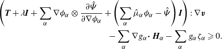 \begin{align} \left (\boldsymbol{T} + \lambda \boldsymbol{I} +\sum _{\alpha } \nabla \phi _\alpha \otimes \frac {\partial \hat {\Psi }}{\partial \nabla \phi _\alpha } +\left (\sum _{\alpha } \hat {\mu }_\alpha \phi _\alpha - \hat {\Psi }\right )\boldsymbol{I}\right ):\nabla \boldsymbol{v}&\nonumber \\ - \sum _{\alpha }\nabla g_\alpha {\boldsymbol\cdot}\ \boldsymbol{H}_\alpha -\sum _{\alpha } g_\alpha \zeta _\alpha &\geqslant 0. \end{align}
Remark 3.8 (Compatibility with continuum mixture theory). This section has demonstrated that the energy-dissipation postulate (3.3) is fulfilled when the local inequality (3.21) is satisfied. As mentioned in Remark 3.2, the energy-dissipation postulate is an approximation of the second law of mixture theory. However, we emphasise that the presented derivations are fully compatible with continuum mixture theory.
We finalise this section with a remark on the connection between the chemical potentials and the Lagrange multiplier. Directly enforcing the saturation constraint (2.5b ) provides
 \begin{align} \lambda + \sum _{\alpha }\hat {\mu }_\alpha \phi _\alpha = \sum _\alpha \hat {\mu }_{\alpha ,\lambda } \phi _\alpha . \end{align}
This observation reveals that chemical potentials in (3.21) occur solely in the form $\hat {\mu }_{\alpha ,\lambda }$
. In other words, the chemical potentials
$\hat {\mu }_{\alpha ,\lambda }$
. In other words, the chemical potentials $\hat {\mu }_\alpha$
are tightly connected with the Lagrange multiplier
$\hat {\mu }_\alpha$
are tightly connected with the Lagrange multiplier $\lambda$
. This is consistent with the examination that the addition of
$\lambda$
. This is consistent with the examination that the addition of $\sum _\alpha \phi _\alpha - 1$
should not alter the free energy. Indeed, we have
$\sum _\alpha \phi _\alpha - 1$
should not alter the free energy. Indeed, we have
 \begin{align} \Psi =&\, \hat {\Psi }\left (\left \{\phi _\alpha \right \}_{\alpha =1,\ldots ,N},\left \{\nabla \phi _\alpha \right \}_{\alpha =1,\ldots ,N}\right ) + \lambda \left (\sum _\alpha \phi _\alpha -1 \right ), \end{align}
and the associated chemical potential quantities ( $\alpha = 1,\ldots ,N$
) naturally include the Lagrange multiplier
$\alpha = 1,\ldots ,N$
) naturally include the Lagrange multiplier $\lambda$
:
$\lambda$
:
 \begin{align} \hat {\mu }_{\alpha ,\lambda } = \frac { \partial \Psi }{\partial \phi _\alpha } - \textrm{div}\frac {\partial \Psi }{\partial \nabla \phi _\alpha }, \end{align}
where we recall (3.19b ). We do not directly enforce (2.5b ) and continue with the left-hand side of (3.22).
3.3. Alternative free energy classes
As mentioned in Remark3.4, as an alternative for (3.5), we explore the approach of working with a class that depends on concentration. This exploration is motivated by its occurrence in the literature on two-phase models (e.g. Lowengrub & Truskinovsky Reference Lowengrub and Truskinovsky1998). We consider the following constitutive class:
 \begin{align} \Psi =&\, \check {\Psi }\left (\left \{c_\alpha \right \},\left \{\nabla c_\alpha \right \}\right ), \end{align}
subject to the summation constraint (2.5a
). Alongside free energy class (3.25), we introduce the chemical potential quantities ( $\alpha = 1,\ldots ,N$
):
$\alpha = 1,\ldots ,N$
):
 \begin{align} \check {\mu }_\alpha =&\, \frac { \partial \hat {\Psi }}{\partial c_\alpha } - \textrm{div}\frac {\partial \hat {\Psi }}{\partial \nabla c_\alpha }. \end{align}
In Appendix C we provide the derivation of the modelling restriction that emerges from the constitutive class (3.25). The modelling restriction takes the form
 \begin{align} \left (\boldsymbol{T} + \check {\lambda }\boldsymbol{I} +\sum _{\alpha } \nabla c_\alpha \otimes \frac {\partial \check {\Psi }}{\partial \nabla c_\alpha } - \check {\Psi }\boldsymbol{I}\right ):\nabla \boldsymbol{v}&\nonumber \\ - \sum _{\alpha }\nabla \left ( \rho ^{-1}\check {\mu }_\alpha + \rho _\alpha ^{-1}\check {\lambda } \right ){\boldsymbol\cdot}\ \boldsymbol{H}_\alpha -\sum _{\alpha } \left ( \rho ^{-1}\check {\mu }_\alpha + \rho _\alpha ^{-1}\check {\lambda } \right ) \zeta _\alpha &\geqslant 0, \end{align}
where $\check {\lambda }$
is the Lagrange multiplier associated with the constraint (2.29b
). Noting that the volume fractions and concentrations are connected via (2.7):
$\check {\lambda }$
is the Lagrange multiplier associated with the constraint (2.29b
). Noting that the volume fractions and concentrations are connected via (2.7):
 \begin{align} \phi _\alpha =&\, \phi _\alpha ( \{c_{\beta } \}), \end{align}
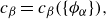 \begin{align} c_{\beta } =&\, c_{\beta }(\{\phi _\alpha \}), \end{align}
the identification
 \begin{align} \hat {\Psi }(\{\phi _\alpha\}) =\check {\Psi }(\{c_{\beta }\}) \end{align}
reveals that the free energy classes coincide. Given that the initial modelling restriction is the same for both classes, we conclude that the resulting modelling restrictions must coincide as well. In other words, the modelling restriction is independent of the choice of order parameters.
Theorem 3.9 (Equivalence of modelling restrictions). The modelling restrictions(3.21)and(3.27)are equivalent.
For an alternative path to show equivalence of the modelling restrictions, one could apply the variable transformation (3.28) defined in (2.7) to show that (3.27) coincides with (3.21). We discuss this approach in Appendix B.
Guided by Theorem3.9, we proceed with the formulation of the modelling restriction presented in (3.21).
3.4. Selection of constitutive models
By means of the Colemann–Noll concept, we utilise (3.21) as a guiding principle to design constitutive models. Inspired by the specific form of the constraint (3.21), we restrict ourselves to mixture stress tensors $\boldsymbol{T}$
, constituent peculiar velocities
$\boldsymbol{T}$
, constituent peculiar velocities $\boldsymbol{J}_\alpha$
, and constituent mass transfer terms
$\boldsymbol{J}_\alpha$
, and constituent mass transfer terms $\boldsymbol{j}_\alpha , \zeta _\alpha$
that belong to the constitutive classes:
$\boldsymbol{j}_\alpha , \zeta _\alpha$
that belong to the constitutive classes:
 \begin{align} \boldsymbol{T} =&\, \hat {\boldsymbol{T}}\left (\nabla \boldsymbol{v}, \left \{\phi _\alpha \right \}, \left \{\nabla \phi _\alpha \right \}, \left \{g_{\alpha }\right \}, \left \{\nabla g_{\alpha }\right \}\right ), \end{align}
 \begin{align} \boldsymbol{J}_\alpha =&\, \hat {\boldsymbol{J}}_\alpha \left (\left \{\phi _\alpha \right \}, \left \{\nabla g_\alpha \right \}\right ), \end{align}
 \begin{align} \boldsymbol{j}_\alpha =&\, \hat {\boldsymbol{j}}_\alpha \left (\left \{\phi _\alpha \right \}, \left \{\nabla g_\alpha \right \}\right ), \end{align}
 \begin{align} \zeta _\alpha =&\, \hat {\zeta }_\alpha \left (\left \{\phi _\alpha \right \}, \left \{g_\alpha \right \}\right ), \end{align}
and define $\hat {\boldsymbol{H}}_\alpha = \hat {\boldsymbol{J}}_\alpha + \hat {\boldsymbol{j}}_\alpha$
. Generally speaking, the introduction of the class (3.30b
) deviates from continuum mixture theory. Arguably, a natural approximation is simply taking
$\hat {\boldsymbol{H}}_\alpha = \hat {\boldsymbol{J}}_\alpha + \hat {\boldsymbol{j}}_\alpha$
. Generally speaking, the introduction of the class (3.30b
) deviates from continuum mixture theory. Arguably, a natural approximation is simply taking $\hat {\boldsymbol{J}}_\alpha = 0$
, which, for instance, models the situation of matching velocities
$\hat {\boldsymbol{J}}_\alpha = 0$
, which, for instance, models the situation of matching velocities $\boldsymbol{v}_\alpha =\boldsymbol{v}_{\beta }$
. We return to this case in § 4.2.
$\boldsymbol{v}_\alpha =\boldsymbol{v}_{\beta }$
. We return to this case in § 4.2.
We do not seek the most complete constitutive theory, rather our goal is to find a set of practical constitutive models compatible with (3.21). To this end, we aim to identify constitutive models (3.30) so that all three terms in (3.21) are positive, which occurs when
 \begin{align} \left (\boldsymbol{T} + \lambda \boldsymbol{I} +\sum _{\alpha } \nabla \phi _\alpha \otimes \frac {\partial \hat {\Psi }}{\partial \nabla \phi _\alpha } +\left (\sum _{\alpha } \hat {\mu }_{\alpha }\phi _\alpha - \hat {\Psi }\right )\boldsymbol{I}\right ):\nabla \boldsymbol{v}&\geqslant 0, \end{align}
 \begin{align} -\sum _{\alpha }\nabla g_\alpha {\boldsymbol\cdot}\ \boldsymbol{J}_\alpha &\geqslant 0, \end{align}
 \begin{align} -\sum _{\alpha }\nabla g_\alpha {\boldsymbol\cdot}\ \boldsymbol{j}_\alpha &\geqslant 0, \end{align}
 \begin{align} -\sum _{\alpha } g_\alpha \zeta _\alpha &\geqslant 0. \end{align}
Remark 3.10 (Onsager reciprocal relations). As mentioned earlier, our objective is to find a set of practical constitutive models. A more complete theory follows from working with the original constraint (3.21), and extending the dependency of the classes (3.30). In particular, the classes may be interconnected. The well-known Onsager reciprocal relations take a central place in this framework. We refer to Onsager (Reference Onsager1931a,Reference Onsagerb).
In the following, we provide constitutive models for the mixture stress tensor, constituent peculiar velocities and constituent mass transfer, respectively.
Mixture stress tensor. We select the following constitutive model for the stress tensor:
 \begin{align} \hat {\boldsymbol{T}} = -\lambda \boldsymbol{I}-\sum _{\alpha } \nabla \phi _\alpha \otimes \frac {\partial \hat {\Psi }}{\partial \nabla \phi _\alpha }-\left (\sum _{\alpha } \hat {\mu }_{\alpha }\phi _\alpha - \hat {\Psi }\right )\boldsymbol{I} + \nu (2\nabla ^s \boldsymbol{v}+\bar {\lambda }(\textrm{div}\boldsymbol{v}) \boldsymbol{I}), \end{align}
subject to the symmetry condition
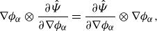 \begin{align} \nabla \phi _\alpha \otimes \frac {\partial \hat {\Psi }}{\partial \nabla \phi _\alpha } = \frac {\partial \hat {\Psi }}{\partial \nabla \phi _\alpha } \otimes \nabla \phi _\alpha , \end{align}
where the scalar field $\nu \geqslant 0$
is the mixture dynamic viscosity,
$\nu \geqslant 0$
is the mixture dynamic viscosity, $\bar {\lambda } \geqslant -2/d$
is a scalar, and
$\bar {\lambda } \geqslant -2/d$
is a scalar, and $d$
is the number of dimensions. Possible choices for the mixture viscosity include
$d$
is the number of dimensions. Possible choices for the mixture viscosity include $\nu = \sum _\alpha \nu _\alpha \phi _\alpha$
and
$\nu = \sum _\alpha \nu _\alpha \phi _\alpha$
and $\nu = \sum _\alpha \nu _\alpha c_\alpha$
, where
$\nu = \sum _\alpha \nu _\alpha c_\alpha$
, where $\nu _\alpha$
are constituent viscosities. The condition (3.33) ensures compatibility with the angular momentum constraint (2.25c
).
$\nu _\alpha$
are constituent viscosities. The condition (3.33) ensures compatibility with the angular momentum constraint (2.25c
).
Lemma 3.11 (Compatibility mixture stress tensor). The mixture stress tensor(3.32)adheres to the constraint(3.31a).
Proof. An elementary calculation gives
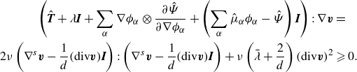 \begin{align} \left (\hat {\boldsymbol{T}} +\lambda \boldsymbol{I} +\sum _{\alpha } \nabla \phi _\alpha \otimes \frac {\partial \hat {\Psi }}{\partial \nabla \phi _\alpha } +\left (\sum _{\alpha } \hat {\mu }_{\alpha }\phi _\alpha - \hat {\Psi }\right )\boldsymbol{I}\right ):\nabla \boldsymbol{v} &= \nonumber \\ 2 \nu \left ( \nabla ^s \boldsymbol{v} - \frac {1}{d} (\textrm{div} \boldsymbol{v}) \boldsymbol{I}\right ):\left (\nabla ^s \boldsymbol{v} - \frac {1}{d} (\textrm{div} \boldsymbol{v}) \boldsymbol{I}\right ) + \nu \left (\bar {\lambda } + \frac {2}{d}\right )\left (\textrm{div} \boldsymbol{v}\right )^2 &\geqslant 0. \end{align}
Constituent peculiar velocities. We choose the peculiar velocities of the form
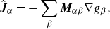 \begin{align} \hat {\boldsymbol{J}}_\alpha = -\sum _{\beta } \boldsymbol{M}_{\alpha {\beta }} \nabla g_{\beta }, \end{align}
with mobility tensor $\boldsymbol{M}_{\alpha {\beta }}=\boldsymbol{M}_{{\beta }\alpha }$
. The mobility tensor is positive definite (
$\boldsymbol{M}_{\alpha {\beta }}=\boldsymbol{M}_{{\beta }\alpha }$
. The mobility tensor is positive definite ( $\boldsymbol{y}_\alpha ^{T} \boldsymbol{M}_{\alpha {\beta }}\boldsymbol{y}_{\beta } \geqslant 0$
for all
$\boldsymbol{y}_\alpha ^{T} \boldsymbol{M}_{\alpha {\beta }}\boldsymbol{y}_{\beta } \geqslant 0$
for all $\boldsymbol{y}_\alpha \in \mathbb{R}^d, \alpha = 1,\ldots ,N$
), has the same dependencies as (3.31b
), is compatible with
$\boldsymbol{y}_\alpha \in \mathbb{R}^d, \alpha = 1,\ldots ,N$
), has the same dependencies as (3.31b
), is compatible with $\sum _\alpha \boldsymbol{M}_{\alpha {\beta }} = \sum _\alpha \boldsymbol{M}_{{\beta }\alpha } = 0$
for all
$\sum _\alpha \boldsymbol{M}_{\alpha {\beta }} = \sum _\alpha \boldsymbol{M}_{{\beta }\alpha } = 0$
for all ${\beta }=1,..,N$
, and vanishes in the single fluid region
${\beta }=1,..,N$
, and vanishes in the single fluid region $\boldsymbol{M}_{\alpha {\beta }}|_{\phi _{\gamma }=1}=0, {\gamma } =1,\ldots ,N$
(thus is degenerate). We note that the symmetry requirement follows from the Onsager reciprocal relations, the positive definiteness from (3.31b
), and the zero sum of rows and columns from (3.2a
). A possible choice for the mobility tensor is
$\boldsymbol{M}_{\alpha {\beta }}|_{\phi _{\gamma }=1}=0, {\gamma } =1,\ldots ,N$
(thus is degenerate). We note that the symmetry requirement follows from the Onsager reciprocal relations, the positive definiteness from (3.31b
), and the zero sum of rows and columns from (3.2a
). A possible choice for the mobility tensor is $\boldsymbol{M}_{\alpha {\beta }}=-\boldsymbol{M}_0 \tilde {\rho }_\alpha \tilde {\rho }_{\beta }$
for
$\boldsymbol{M}_{\alpha {\beta }}=-\boldsymbol{M}_0 \tilde {\rho }_\alpha \tilde {\rho }_{\beta }$
for $\alpha \neq {\beta }$
, and
$\alpha \neq {\beta }$
, and $\boldsymbol{M}_{\alpha \alpha } = \boldsymbol{M}_{0}\tilde {\rho }_\alpha \sum _{{\gamma }\neq \alpha } \tilde {\rho }_{\gamma }$
for some
$\boldsymbol{M}_{\alpha \alpha } = \boldsymbol{M}_{0}\tilde {\rho }_\alpha \sum _{{\gamma }\neq \alpha } \tilde {\rho }_{\gamma }$
for some $\boldsymbol{M}_0$
that does not depend on the constituent number.
$\boldsymbol{M}_0$
that does not depend on the constituent number.
Remark 3.12 (Lagrange multiplier in constituent peculiar velocities). In most incompressible $N$
-phase models, the Lagrange multiplier
$N$
-phase models, the Lagrange multiplier $\lambda$
does not explicitly appear in the constituent peculiar velocities
$\lambda$
does not explicitly appear in the constituent peculiar velocities $\hat {\boldsymbol{J}}_\alpha$
, whereas in the proposed framework, it appears as a component of
$\hat {\boldsymbol{J}}_\alpha$
, whereas in the proposed framework, it appears as a component of $g_\alpha$
. Notably, when all constituent densities are identical (
$g_\alpha$
. Notably, when all constituent densities are identical ( $\rho _\alpha = \rho$
for
$\rho _\alpha = \rho$
for $\alpha =1,\ldots ,N$
), the Lagrange multiplier vanishes, yielding the relation
$\alpha =1,\ldots ,N$
), the Lagrange multiplier vanishes, yielding the relation $g_\alpha - g_{\beta } = \rho ^{-1}(\hat {\mu }_\alpha -\hat {\mu }_{\beta })$
.
$g_\alpha - g_{\beta } = \rho ^{-1}(\hat {\mu }_\alpha -\hat {\mu }_{\beta })$
.
Lemma 3.13 (Compatibility constituent peculiar velocities). The choice(3.35)aligns with both the balance(2.13)and the restriction(3.31b).
Constituent diffusive flux. Analogously to the constituent peculiar velocities, we select
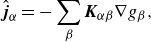 \begin{align} \hat {\boldsymbol{j}}_\alpha = -\sum _{\beta } \boldsymbol{K}_{\alpha {\beta }} \nabla g_{\beta }, \end{align}
for some positive definite constitutive tensor $\boldsymbol{K}_{\alpha {\beta }}=\boldsymbol{K}_{{\beta }\alpha }$
compatible with
$\boldsymbol{K}_{\alpha {\beta }}=\boldsymbol{K}_{{\beta }\alpha }$
compatible with $\sum _\alpha \boldsymbol{K}_{\alpha {\beta }}=\sum _\alpha \boldsymbol{K}_{{\beta }\alpha }=0$
, with the same dependencies as (3.30c
), and which vanishes in the single fluid region
$\sum _\alpha \boldsymbol{K}_{\alpha {\beta }}=\sum _\alpha \boldsymbol{K}_{{\beta }\alpha }=0$
, with the same dependencies as (3.30c
), and which vanishes in the single fluid region $\boldsymbol{K}_{\alpha {\beta }}|_{\phi _{\gamma }=1}=0, {\gamma } =1,\ldots ,N$
. Similarly as for the peculiar velocity, a possible choice for the mobility tensor is
$\boldsymbol{K}_{\alpha {\beta }}|_{\phi _{\gamma }=1}=0, {\gamma } =1,\ldots ,N$
. Similarly as for the peculiar velocity, a possible choice for the mobility tensor is $\boldsymbol{K}_{\alpha {\beta }}=-\boldsymbol{K}_0 \tilde {\rho }_\alpha \tilde {\rho }_{\beta }$
for
$\boldsymbol{K}_{\alpha {\beta }}=-\boldsymbol{K}_0 \tilde {\rho }_\alpha \tilde {\rho }_{\beta }$
for $\alpha \neq {\beta }$
, and
$\alpha \neq {\beta }$
, and $\boldsymbol{K}_{\alpha \alpha } = \boldsymbol{K}_{0}\tilde {\rho }_\alpha \sum _{{\gamma }\neq \alpha } \tilde {\rho }_{\gamma }$
for some
$\boldsymbol{K}_{\alpha \alpha } = \boldsymbol{K}_{0}\tilde {\rho }_\alpha \sum _{{\gamma }\neq \alpha } \tilde {\rho }_{\gamma }$
for some $\boldsymbol{K}_0$
that is not dependent on the constituent number.
$\boldsymbol{K}_0$
that is not dependent on the constituent number.
Lemma 3.14 (Compatibility constituent diffusive fluxes). The choice(3.36)aligns with both the balance(2.28b)and the restriction(3.31c).
Constituent mass transfer. We select the constituent mass transfer terms analogously to the constituent peculiar velocities:
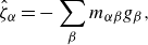 \begin{align} \hat {\zeta }_\alpha = -\sum _{\beta } m_{\alpha {\beta }} g_{\beta }, \end{align}
where the positive definite scalar mobility $m_{\alpha {\beta }}=m_{{\beta }\alpha }$
has the same dependencies as (3.30d
), is compatible with
$m_{\alpha {\beta }}=m_{{\beta }\alpha }$
has the same dependencies as (3.30d
), is compatible with $\sum _\alpha m_{\alpha {\beta }} = \sum _\alpha m_{{\beta }\alpha } = 0$
, and vanishes in the single fluid region
$\sum _\alpha m_{\alpha {\beta }} = \sum _\alpha m_{{\beta }\alpha } = 0$
, and vanishes in the single fluid region $m_{\alpha {\beta }}|_{\phi _{\gamma }=1}=0, {\gamma } =1,\ldots ,N$
.
$m_{\alpha {\beta }}|_{\phi _{\gamma }=1}=0, {\gamma } =1,\ldots ,N$
.
Lemma 3.15 (Compatibility mass transfer). The choice(3.37)is compatible with the balance of mass supply(2.27b)and the constraint(3.31d).
Remark 3.16 (Related constitutive models). In the case,
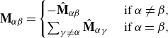 \begin{align} \textbf{M}_{\alpha {\beta }} = \begin{cases} -\hat {\textbf{M}}_{\alpha {\beta }} & \text{ if }\alpha \neq {\beta },\\ \sum _{{\gamma }\neq \alpha } \hat {\textbf{M}}_{\alpha {\gamma }} & \text{ if }\alpha = {\beta }, \end{cases} \end{align}
for some symmetric $\hat {\textbf{M}}_{\alpha {\beta }}$
, we find
$\hat {\textbf{M}}_{\alpha {\beta }}$
, we find
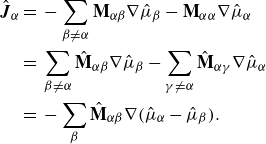 \begin{align} \hat {\boldsymbol{J}}_\alpha =&\, - \sum _{{\beta }\neq \alpha } \textbf{M}_{\alpha {\beta }}\nabla \hat {\mu }_{\beta } - \textbf{M}_{\alpha \alpha }\nabla \hat {\mu }_\alpha \nonumber \\ =&\, \sum _{{\beta }\neq \alpha } \hat {\textbf{M}}_{\alpha {\beta }}\nabla \hat {\mu }_{\beta } - \sum _{{\gamma }\neq \alpha }\hat {\textbf{M}}_{\alpha {\gamma }}\nabla \hat {\mu }_\alpha \nonumber \\ =&\, -\sum _{{\beta }} \hat {\textbf{M}}_{\alpha {\beta }}\nabla (\hat {\mu }_\alpha -\hat {\mu }_{\beta }). \end{align}
This model matches (for the isotropic case $\textbf{M}_{\alpha {\beta }} = {\rm M}_{\alpha {\beta }}\textbf{I}$
) that of ten Eikelder et al. (Reference ten Eikelder, van der Zee and Schillinger2024). It also closely resembles the form adopted in Li & Wang (Reference Li and Wang2014). Both closure models involve the Lagrange multiplier
$\textbf{M}_{\alpha {\beta }} = {\rm M}_{\alpha {\beta }}\textbf{I}$
) that of ten Eikelder et al. (Reference ten Eikelder, van der Zee and Schillinger2024). It also closely resembles the form adopted in Li & Wang (Reference Li and Wang2014). Both closure models involve the Lagrange multiplier $\lambda$
; a difference lies in the fact that the model proposed by Li & Wang (Reference Li and Wang2014) depends on the numbering of the constituents. Finally, we note that forms similar to (3.39) may be adopted for the diffusive fluxes and the mass transfer terms.
$\lambda$
; a difference lies in the fact that the model proposed by Li & Wang (Reference Li and Wang2014) depends on the numbering of the constituents. Finally, we note that forms similar to (3.39) may be adopted for the diffusive fluxes and the mass transfer terms.
This finalises the construction of constitutive models compatible with the imposed energy-dissipative postulate. Substitution of the models (3.32), (3.35) and (3.37) yields the class of incompressible $N$
-phase models:
$N$
-phase models:
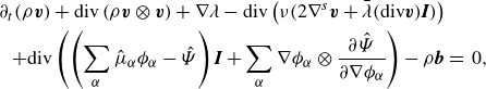 \begin{align} \partial _t (\rho \boldsymbol{v}) + \textrm{div} \left ( \rho \boldsymbol{v}\otimes \boldsymbol{v} \right ) + \nabla \lambda - \textrm{div} \left ( \nu (2\nabla ^s \boldsymbol{v}+\bar {\lambda }(\textrm{div}\boldsymbol{v}) \boldsymbol{I}) \right )& \nonumber \\ + \textrm{div} \left (\left (\sum _\alpha \hat {\mu }_\alpha \phi _\alpha -\hat {\Psi }\right )\boldsymbol{I} + \sum _\alpha \nabla \phi _\alpha \otimes \frac {\partial \hat {\Psi }}{\partial \nabla \phi _\alpha } \right )-\rho \boldsymbol{b}&=\, 0, \end{align}
 \begin{align} \partial _t \phi _\alpha + \textrm{div}(\phi _\alpha \boldsymbol{v}) + \rho _\alpha ^{-1}\textrm{div}\hat {\boldsymbol{J}}_\alpha + \rho _\alpha ^{-1}\textrm{ div}\hat {\boldsymbol{j}}_\alpha - \hat {\zeta }_\alpha &=\,0, \end{align}
 \begin{align} \textrm{div} \boldsymbol{v} + \sum _\alpha \rho ^{-1}_\alpha \textrm{div}(\hat {\boldsymbol{J}}_\alpha + \hat {\boldsymbol{j}}_\alpha ) - \rho ^{-1}_\alpha \hat {\zeta }_\alpha &=\,0, \end{align}
 \begin{align} \hat {\mu }_\alpha - \frac {\partial \hat {\Psi }}{\partial \phi _\alpha } + \textrm{div} \left ( \frac {\partial \hat {\Psi }}{\partial \nabla \phi _\alpha } \right )&=\,0, \end{align}
 \begin{align} \hat {\boldsymbol{J}}_\alpha + \sum _{\beta } \boldsymbol{M}_{\alpha {\beta }} \nabla g_{\beta }&\,=0, \end{align}
 \begin{align} \hat {\boldsymbol{j}}_\alpha + \sum _{\beta } \boldsymbol{K}_{\alpha {\beta }}\nabla g_{\beta } &\,=0, \end{align}
 \begin{align} \hat {\zeta }_\alpha + \sum _{\beta } m_{\alpha {\beta }} g_{\beta } &\,=0, \end{align}
where (3.40b
) and (3.40c
) and the initial condition $\sum _{\beta } \phi _{{\beta }}(\boldsymbol{x},t=0) =1$
together ensure
$\sum _{\beta } \phi _{{\beta }}(\boldsymbol{x},t=0) =1$
together ensure $\sum _{\beta } \phi _{{\beta }}(\boldsymbol{x},t) =1$
. Formulation (3.40) constitutes a class of models in the sense that particular closure relations (
$\sum _{\beta } \phi _{{\beta }}(\boldsymbol{x},t) =1$
. Formulation (3.40) constitutes a class of models in the sense that particular closure relations ( $\boldsymbol{M}_{\alpha {\beta }}$
,
$\boldsymbol{M}_{\alpha {\beta }}$
, $\boldsymbol{K}_{\alpha {\beta }}$
,
$\boldsymbol{K}_{\alpha {\beta }}$
, $m_{\alpha {\beta }}$
and
$m_{\alpha {\beta }}$
and $\Psi$
) need to be specified. A possible Cahn–Hilliard-type free energy is
$\Psi$
) need to be specified. A possible Cahn–Hilliard-type free energy is $\hat {\Psi }=\Psi _0(\left \{\phi _\alpha \right \})+{1}/{2}\sum _{\alpha {\beta }} \sigma _{\alpha {\beta }}\nabla \phi _\alpha {\boldsymbol\cdot} \nabla \phi _{\beta }$
, with
$\hat {\Psi }=\Psi _0(\left \{\phi _\alpha \right \})+{1}/{2}\sum _{\alpha {\beta }} \sigma _{\alpha {\beta }}\nabla \phi _\alpha {\boldsymbol\cdot} \nabla \phi _{\beta }$
, with $\sigma$
positive semidefinite. Given these relations, (3.40) is a well-defined closed model; this model is invariant to the renumbering of the constituents, invariant to the set of independent variables, and reduction-consistent. Additionally, it exhibits energy dissipation, which we state explicitly in the following theorem.
$\sigma$
positive semidefinite. Given these relations, (3.40) is a well-defined closed model; this model is invariant to the renumbering of the constituents, invariant to the set of independent variables, and reduction-consistent. Additionally, it exhibits energy dissipation, which we state explicitly in the following theorem.
Theorem 3.17 (Compatibility energy dissipation). The model (3.40) is compatible with the energy-dissipation condition(3.3).
Proof. This follows from Lemma3.11, Lemma3.13 and Lemma3.15. In particular, the dissipation takes the form
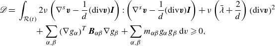 \begin{align} \mathscr{D} = &\, \displaystyle \int _{\mathcal{R}(t)} 2 \nu \left ( \nabla ^s \boldsymbol{v} - \frac {1}{d} (\textrm{div} \boldsymbol{v}) \boldsymbol{I}\right ):\left (\nabla ^s \boldsymbol{v} - \frac {1}{d} (\textrm{div} \boldsymbol{v}) \boldsymbol{I}\right )+ \nu \left (\bar\lambda + \frac {2}{d}\right )\left (\textrm{div} \boldsymbol{v}\right )^2 \nonumber \\ &\,\quad \quad + \displaystyle \sum _{\alpha ,{\beta }} \left (\nabla g_\alpha \right )^{T} \boldsymbol{B}_{\alpha {\beta }} \nabla g_{\beta }+ \sum _{\alpha ,{\beta }} m_{\alpha {\beta }}g_\alpha g_{\beta }\,\textrm{d}v \geqslant 0, \end{align}
with $\boldsymbol{B}_{\alpha {\beta }}=\boldsymbol{M}_{\alpha {\beta }}+\boldsymbol{K}_{\alpha {\beta }}$
.
$\boldsymbol{B}_{\alpha {\beta }}=\boldsymbol{M}_{\alpha {\beta }}+\boldsymbol{K}_{\alpha {\beta }}$
.
4. Model characteristics
In this section, we explore the characteristics of the modelling framework outlined in § 3. To this end, we discuss alternative – equivalent – formulations in § 4.1. We present the case of matching velocities in § 4.2. Subsequently, § 4.3 details the equilibrium characteristics.
4.1. Alternative formulations
As discussed in § 2 and § 3, the unified modelling framework outlined in these sections is invariant to the choice of variables. However, it is worthwhile to discuss some of the formulations that are associated with particular variables.
First, we note that one can identify a pressure quantity in the model as
 \begin{align} p: = \sum _\alpha \hat {\mu }_\alpha \phi _\alpha -\hat {\Psi }. \end{align}
With this choice, the model takes the more compact form:
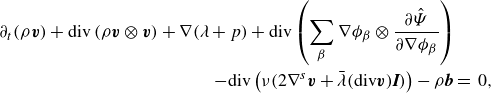 \begin{align} \partial _t (\rho \boldsymbol{v}) + \textrm{div} \left ( \rho \boldsymbol{v}\otimes \boldsymbol{v} \right ) + \nabla (\lambda + p) + \textrm{div} \left ( \sum _{\beta } \nabla \phi _{\beta } \otimes \frac {\partial \hat {\Psi }}{\partial \nabla \phi _{\beta }} \right )& \nonumber \\ - \textrm{div} \left ( \nu (2\nabla ^s \boldsymbol{v}+\bar {\lambda }(\textrm{div}\boldsymbol{v}) \boldsymbol{I}) \right )-\rho \boldsymbol{b} &=\, 0, \end{align}
 \begin{align} \partial _t \phi _\alpha + \textrm{div}(\phi _\alpha \boldsymbol{v}) + \rho _\alpha ^{-1}\textrm{div}\hat {\boldsymbol{H}}_\alpha - \hat {\zeta }_\alpha &=\,0, \end{align}
 \begin{align} \textrm{div} \boldsymbol{v} + \sum _\alpha \rho ^{-1}_\alpha \textrm{div}(\hat {\boldsymbol{J}}_\alpha + \hat {\boldsymbol{j}}_\alpha ) - \rho ^{-1}_\alpha \hat {\zeta }_\alpha &=\,0. \end{align}
In accordance with the first metaphysical principle of continuum mixture theory, the mixture free energy comprises constituent free energies:
 \begin{align} \hat {\Psi } = \sum _\alpha \hat {\Psi }_\alpha , \end{align}
where $\hat {\Psi }_\alpha$
are the volume-measure constituent free energies. Utilising (4.3) we observe that the pressure satisfies Dalton’s law:
$\hat {\Psi }_\alpha$
are the volume-measure constituent free energies. Utilising (4.3) we observe that the pressure satisfies Dalton’s law:
 \begin{align} p = &\, \sum _\alpha p_\alpha , \end{align}
 \begin{align} p_\alpha = &\, \sum _{{\beta }}\hat {\mu }_{\alpha {\beta }} \phi _{\beta } - \hat {\Psi }_\alpha , \end{align}
where $p_\alpha$
is the partial pressure of constituent
$p_\alpha$
is the partial pressure of constituent $\alpha$
with
$\alpha$
with $\hat {\mu }_{\alpha {\beta }}=\partial _{\phi _{\beta }}\hat {\Psi }_\alpha - \textrm{div}\partial _{\nabla \phi _{\beta }}\hat {\Psi }_\alpha$
. Thus, the split (4.3) reveals that the system may be written as
$\hat {\mu }_{\alpha {\beta }}=\partial _{\phi _{\beta }}\hat {\Psi }_\alpha - \textrm{div}\partial _{\nabla \phi _{\beta }}\hat {\Psi }_\alpha$
. Thus, the split (4.3) reveals that the system may be written as
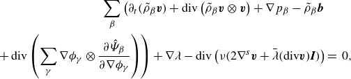 \begin{align} \sum _{\beta } \left ( \partial _t (\tilde {\rho }_{\beta } \boldsymbol{v}) + \textrm{div} \left ( \tilde {\rho }_{\beta } \boldsymbol{v}\otimes \boldsymbol{v} \right ) + \nabla p_{\beta } -\tilde {\rho }_{\beta } \boldsymbol{b} \right . &\nonumber \\ \left .+\, \textrm{div} \left ( \sum _{\gamma } \nabla \phi _{\gamma } \otimes \frac {\partial \hat {\Psi }_{\beta }}{\partial \nabla \phi _{\gamma }} \right )\right ) +\nabla \lambda - \textrm{div} \left ( \nu (2\nabla ^s \boldsymbol{v}+\bar\lambda (\textrm{div}\boldsymbol{v}) \boldsymbol{I}) \right ) &=\, 0, \end{align}
 \begin{align} \partial _t \phi _\alpha + \textrm{div}(\phi _\alpha \boldsymbol{v}) + \rho _\alpha ^{-1}\textrm{div}\hat {\boldsymbol{H}}_\alpha - \hat {\zeta }_\alpha &=\,0, \end{align}
 \begin{align} \textrm{div} \boldsymbol{v} + \sum _\alpha \rho ^{-1}_\alpha \textrm{div}(\hat {\boldsymbol{J}}_\alpha + \hat {\boldsymbol{j}}_\alpha ) - \rho ^{-1}_\alpha \hat {\zeta }_\alpha &=\,0. \end{align}
An alternative compact form is obtained with the aid of the following lemma.
Lemma 4.1 (Identity free energy). The free energy contributions collapse into
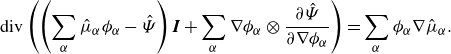 \begin{align} \textrm{div} \left (\left (\sum _\alpha \hat {\mu }_\alpha \phi _\alpha -\hat {\Psi }\right )\boldsymbol{I} + \sum _\alpha \nabla \phi _\alpha \otimes \frac {\partial \hat {\Psi }}{\partial \nabla \phi _\alpha } \right ) = \sum _\alpha \phi _\alpha \nabla \hat {\mu }_\alpha . \end{align}
Proof. See LemmaA.4.
Invoking Lemma4.1, model (3.40) takes a more compact form:
 \begin{align} \partial _t (\rho \boldsymbol{v}) \!+\! \textrm{div} \left ( \rho \boldsymbol{v}\otimes \boldsymbol{v} \right ) \!+\! \nabla \lambda \!+\! \sum _\alpha \phi _\alpha \nabla \hat {\mu }_\alpha - \textrm{div} \left ( \nu (2\nabla ^s \boldsymbol{v}\!+\!\bar {\lambda }(\textrm{div}\boldsymbol{v}) \boldsymbol{I}) \right )-\rho \boldsymbol{b} &= 0, \end{align}
 \begin{align} \partial _t \phi _\alpha + \textrm{div}(\phi _\alpha \boldsymbol{v}) + \rho _\alpha ^{-1}\textrm{div}\hat {\boldsymbol{H}}_\alpha - \hat {\zeta }_\alpha &=\,0, \end{align}
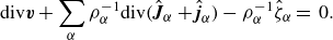 \begin{align} \textrm{div} \boldsymbol{v} + \sum _\alpha \rho ^{-1}_\alpha \textrm{div}(\hat {\boldsymbol{J}}_\alpha + \hat {\boldsymbol{j}}_\alpha ) - \rho ^{-1}_\alpha \hat {\zeta }_\alpha &=\,0. \end{align}
Considering the third and fourth terms in the momentum equation in isolation, when enforcing (2.5b ) these terms can be written as
 \begin{align} \nabla \lambda + \sum _\alpha \phi _\alpha \nabla \hat {\mu }_\alpha = \sum _\alpha \phi _\alpha \nabla (\lambda + \hat {\mu }_\alpha ) = \sum _\alpha \tilde {\rho }_\alpha \nabla g_\alpha . \end{align}
Similarly, in the mass balance (4.7b
), we observe that the chemical potentials $\hat {\mu }_\alpha$
and the Lagrange multiplier
$\hat {\mu }_\alpha$
and the Lagrange multiplier $\lambda$
appear solely as a sum via
$\lambda$
appear solely as a sum via $g_\alpha$
.
$g_\alpha$
.
Additionally, we note that the model can alternatively be written in a form that more closely links to existing phase-field models:
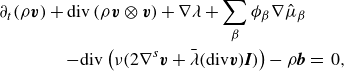 \begin{align} \partial _t (\rho \boldsymbol{v}) + \textrm{div} \left ( \rho \boldsymbol{v}\otimes \boldsymbol{v} \right ) + \nabla \lambda + \sum _{{\beta }} \phi _{\beta }\nabla \hat {\mu }_{\beta } &\nonumber \\ - \textrm{div} \left ( \nu (2\nabla ^s \boldsymbol{v}+\bar {\lambda }(\textrm{div}\boldsymbol{v}) \boldsymbol{I}) \right )-\rho \boldsymbol{b} &=\, 0, \end{align}
 \begin{align} \partial _t \rho + \textrm{div}(\rho \boldsymbol{v}) &=\,0, \end{align}
 \begin{align} \partial _t \phi _\alpha + \textrm{div}(\phi _\alpha \boldsymbol{v}) + \rho _\alpha ^{-1}\textrm{div}\hat {\boldsymbol{H}}_\alpha - \rho _\alpha ^{-1}\hat {\zeta }_\alpha &=\,0, \end{align}
 \begin{align} \textrm{div} \boldsymbol{v} + \sum _\alpha \rho ^{-1}_\alpha \textrm{div}(\hat {\boldsymbol{J}}_\alpha + \hat {\boldsymbol{j}}_\alpha ) - \rho ^{-1}_\alpha \hat {\zeta }_\alpha &=\,0. \end{align}
While we refrain from discussing formulations that adopt concentration variables, we discuss a formulation in terms of the volume-averaged velocity $\boldsymbol{u}$
. Inserting the constitutive model for the peculiar velocities (3.35) into Lemma2.4 we obtain
$\boldsymbol{u}$
. Inserting the constitutive model for the peculiar velocities (3.35) into Lemma2.4 we obtain
 \begin{align} \boldsymbol{v} = \boldsymbol{u} + \rho ^{-1}\displaystyle \sum _{\beta } \hat {\boldsymbol{J}}_{\beta }^u. \end{align}
By substituting this identity, we express the model using the volume-averaged velocity:
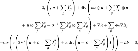 \begin{align} \partial _t \left (\rho \boldsymbol{u} + \sum _{\beta } \hat {\boldsymbol{J}}_{\beta }^u\right ) + \textrm{div} \left ( \rho \boldsymbol{u}\otimes \boldsymbol{u} + \sum _{\beta } \hat {\boldsymbol{J}}_{\beta }^u \otimes \boldsymbol{u} \right .& \nonumber \\+ \left . \boldsymbol{u}\otimes \sum _{\beta } \hat {\boldsymbol{J}}_{\beta }^u + \rho ^{-1} \sum _{\beta } \hat {\boldsymbol{J}}_{\beta }^u\otimes \sum _{\beta } \hat {\boldsymbol{J}}_{\beta }^u\right ) + \nabla \lambda + \sum _{{\beta }} \phi _{\beta }\nabla \hat {\mu }_{\beta } & \nonumber \\- \textrm{div} \! \left ( \nu \! \left (2\nabla ^s \! \left (\boldsymbol{u} +\rho ^{-1} \sum _{\beta } \hat {\boldsymbol{J}}_{\beta }^u \right )+\bar {\lambda }\textrm{ div} \! \left (\boldsymbol{u} +\rho ^{-1} \sum _{\beta } \hat {\boldsymbol{J}}_{\beta }^u \right ) \boldsymbol{I}\right ) \right )-\rho \boldsymbol{b}&=\, 0, \end{align}
 \begin{align} \partial _t \phi _\alpha + \textrm{div}\left (\phi _\alpha \boldsymbol{u}\right )+ \textrm{div}\hat {\boldsymbol{h}}_\alpha ^u + \rho _\alpha ^{-1}\textrm{ div}\hat {\boldsymbol{j}}_\alpha -\rho _\alpha ^{-1}\hat {\zeta }_\alpha &=\,0, \end{align}
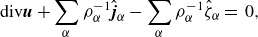 \begin{align} \textrm{div} \boldsymbol{u} +\sum _{\alpha } \rho _\alpha ^{-1} \hat {\boldsymbol{j}}_\alpha -\sum _{\alpha } \rho _\alpha ^{-1}\hat {\zeta }_\alpha &=\,0, \end{align}
where the latter two terms in (4.11c ) vanish when densities match or mass transfer is absent (recall (2.29c )). Arguably, the formulation (4.11) is rather involved. We discuss a simplification in the next subsection.
4.2. Matching velocities
We consider the case in which the peculiar velocities are zero; taking $\boldsymbol{M}_{\alpha {\beta }} = 0$
, we find
$\boldsymbol{M}_{\alpha {\beta }} = 0$
, we find
 \begin{align} \hat {\boldsymbol{J}}_\alpha =\hat {\boldsymbol{h}}_\alpha = \hat {\boldsymbol{J}}_\alpha ^u = \hat {\boldsymbol{h}}_\alpha ^u = 0. \end{align}
As a consequence, the mass-averaged and volume-averaged velocities are equal:
 \begin{align} \boldsymbol{v} = \boldsymbol{u}. \end{align}
This choice models the situation where the constituent velocities are matching. We explicitly state the simplified formulations of the model:
 \begin{align} \partial _t (\rho \boldsymbol{v}) + \textrm{div} \left ( \rho \boldsymbol{v}\otimes \boldsymbol{v} \right ) + \nabla \lambda + \sum _{\beta }\phi _{\beta }\nabla \hat {\mu }_{\beta } &\nonumber \\ - \textrm{div} \left ( \nu (2\nabla ^s \boldsymbol{v}+\bar {\lambda }(\textrm{div}\boldsymbol{v}) \boldsymbol{I}) \right )-\rho \boldsymbol{b} &=\, 0, \end{align}
 \begin{align} \partial _t \phi _\alpha + \textrm{div}(\phi _\alpha \boldsymbol{v}) + \rho _\alpha ^{-1} \textrm{div}\hat {\boldsymbol{j}}_\alpha - \rho _\alpha ^{-1}\hat {\zeta }_\alpha &=\,0, \end{align}
 \begin{align} \textrm{div} \boldsymbol{v} +\sum _{\alpha } \rho _\alpha ^{-1}\textrm{div} \hat {\boldsymbol{j}}_\alpha -\sum _{\alpha } \rho _\alpha ^{-1}\hat {\zeta }_\alpha &=\,0, \end{align}
and, obviously,
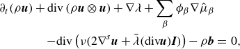 \begin{align} \partial _t (\rho \boldsymbol{u}) + \textrm{div} \left ( \rho \boldsymbol{u}\otimes \boldsymbol{u} \right ) + \nabla \lambda + \sum _{\beta }\phi _{\beta }\nabla \hat {\mu }_{\beta } &\nonumber \\- \textrm{div} \left ( \nu (2\nabla ^s \boldsymbol{u}+\bar {\lambda }(\textrm{div}\boldsymbol{u}) \boldsymbol{I}) \right )-\rho \boldsymbol{b} &=\, 0, \end{align}
 \begin{align} \partial _t \phi _\alpha + \textrm{div}(\phi _\alpha \boldsymbol{u}) + \rho _\alpha ^{-1} \textrm{div}\hat {\boldsymbol{j}}_\alpha - \rho _\alpha ^{-1}\hat {\zeta }_\alpha &=\,0, \end{align}
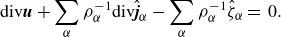 \begin{align} \textrm{div} \boldsymbol{u} +\sum _{\alpha } \rho _\alpha ^{-1}\textrm{div} \hat {\boldsymbol{j}}_\alpha -\sum _{\alpha } \rho _\alpha ^{-1}\hat {\zeta }_\alpha &=\,0. \end{align}
The formulation (4.15) demonstrates that a simplified – consistent – model in terms of the volume-averaged velocity involves a straightforward momentum equation. We emphasise that the volume-averaged velocity $\boldsymbol{u}$
is in general not divergence-free (recall (2.29c
)).
$\boldsymbol{u}$
is in general not divergence-free (recall (2.29c
)).
4.3. Equilibrium conditions
We utilise formulation (4.7) to study equilibrium properties. We characterise the set equilibrium solutions $\left \{\textbf{q}_E=(\boldsymbol{v}_E,\phi _{\alpha ,E},\lambda _E,\mu _{\alpha ,E})\right \}$
of (4.7) as stationary solutions subject to boundary conditions for which the dissipation vanishes:
$\left \{\textbf{q}_E=(\boldsymbol{v}_E,\phi _{\alpha ,E},\lambda _E,\mu _{\alpha ,E})\right \}$
of (4.7) as stationary solutions subject to boundary conditions for which the dissipation vanishes: $\mathscr{D}(\textbf{q}_E) = 0$
. Invoking (3.41) yields the conditions
$\mathscr{D}(\textbf{q}_E) = 0$
. Invoking (3.41) yields the conditions
 \begin{align} \left ( \nabla ^s \boldsymbol{v}_E - \frac {1}{d} (\textrm{div} \boldsymbol{v}_E) \boldsymbol{I}\right ):\left (\nabla ^s \boldsymbol{v}_E - \frac {1}{d} (\textrm{ div} \boldsymbol{v}_E) \boldsymbol{I}\right )=&\,0, \end{align}
 \begin{align} \left (\bar\lambda _E + \frac {2}{d}\right )\left (\textrm{div} \boldsymbol{v}_E\right )^2 =&\,0, \end{align}
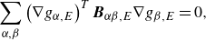 \begin{align} \displaystyle \sum _{\alpha ,{\beta }} \left (\nabla g_{\alpha ,E}\right )^T \boldsymbol{B}_{\alpha {\beta },E} \nabla g_{{\beta },E} =&\,0, \end{align}
 \begin{align} \sum _{\alpha ,{\beta }} m_{\alpha {\beta },E}g_{\alpha ,E}g_{{\beta },E} =&\,0, \end{align}
in $\Omega$
, where
$\Omega$
, where $\boldsymbol{B}_{\alpha {\beta }}=\boldsymbol{M}_{\alpha {\beta }} + \boldsymbol{K}_{\alpha {\beta }}$
, and where the subscript
$\boldsymbol{B}_{\alpha {\beta }}=\boldsymbol{M}_{\alpha {\beta }} + \boldsymbol{K}_{\alpha {\beta }}$
, and where the subscript $E$
denotes the equilibrium configuration of the quantity. We deduce from (4.16a
)–(4.16b
) that
$E$
denotes the equilibrium configuration of the quantity. We deduce from (4.16a
)–(4.16b
) that $\boldsymbol{v}_E$
are rigid body motions. Simplifying the analysis, we take
$\boldsymbol{v}_E$
are rigid body motions. Simplifying the analysis, we take $\boldsymbol{v}_E = 0$
, which causes the inertia terms to vanish. Additionally, we assume the absence of gravitational forces (
$\boldsymbol{v}_E = 0$
, which causes the inertia terms to vanish. Additionally, we assume the absence of gravitational forces ( $\boldsymbol{b} = 0$
). Substituting into the momentum equation (4.7a
) provides
$\boldsymbol{b} = 0$
). Substituting into the momentum equation (4.7a
) provides
 \begin{align} \nabla \lambda _E + \sum _\alpha \phi _{\alpha ,E}\nabla \hat {\mu }_{\alpha ,E} = 0. \end{align}
Recalling (4.8), we deduce
 \begin{align} \sum _\alpha \tilde {\rho }_{\alpha ,E}\nabla g_{\alpha ,E} = 0. \end{align}
Next, from (4.16c
) we deduce that $\nabla g_{E}$
lies in the null space of
$\nabla g_{E}$
lies in the null space of $\boldsymbol{B}_{E}$
in the sense
$\boldsymbol{B}_{E}$
in the sense $\sum _{\beta } \boldsymbol{B}_{\alpha {\beta },E}\nabla g_{{\beta },E} = 0$
(
$\sum _{\beta } \boldsymbol{B}_{\alpha {\beta },E}\nabla g_{{\beta },E} = 0$
( $\alpha = 1,\ldots ,N$
), and hence
$\alpha = 1,\ldots ,N$
), and hence $\hat {\boldsymbol{J}}_{\alpha ,E} + \hat {\boldsymbol{j}}_{\alpha ,E} = 0$
in equilibrium. In the special case
$\hat {\boldsymbol{J}}_{\alpha ,E} + \hat {\boldsymbol{j}}_{\alpha ,E} = 0$
in equilibrium. In the special case $\boldsymbol{B}_{\alpha {\beta }}=-\boldsymbol{B}_0 \tilde {\rho }_\alpha \tilde {\rho }_{\beta }$
for
$\boldsymbol{B}_{\alpha {\beta }}=-\boldsymbol{B}_0 \tilde {\rho }_\alpha \tilde {\rho }_{\beta }$
for $\alpha \neq {\beta }$
, and
$\alpha \neq {\beta }$
, and $\boldsymbol{B}_{\alpha \alpha } = \boldsymbol{B}_{0}\tilde {\rho }_\alpha \sum _{{\gamma }\neq \alpha } \tilde {\rho }_{\gamma }$
for some
$\boldsymbol{B}_{\alpha \alpha } = \boldsymbol{B}_{0}\tilde {\rho }_\alpha \sum _{{\gamma }\neq \alpha } \tilde {\rho }_{\gamma }$
for some $\boldsymbol{B}_0$
that does not depend on
$\boldsymbol{B}_0$
that does not depend on $\tilde {\rho }_\alpha$
,
$\tilde {\rho }_\alpha$
, $\alpha =1,\ldots ,N$
; this coincides with (4.18). Similarly, (4.16d
) provides
$\alpha =1,\ldots ,N$
; this coincides with (4.18). Similarly, (4.16d
) provides $\sum _{\beta } m_{\alpha {\beta },E} g_{{\beta },E} = 0$
, and hence
$\sum _{\beta } m_{\alpha {\beta },E} g_{{\beta },E} = 0$
, and hence $\hat {\zeta }_{\alpha ,E}=0$
(
$\hat {\zeta }_{\alpha ,E}=0$
( $\alpha = 1,\ldots ,N$
).
$\alpha = 1,\ldots ,N$
).
5. Connections to existing models
This section provides connections with existing models. First, we discuss the binary-phase situation in § 5.1. Next, in § 5.2 we compare the framework with the model of Dong (Reference Dong2018). Finally, § 5.3 discusses the link to a model with $N$
-momentum equations.
$N$
-momentum equations.
5.1. Binary-phase case
In this section, we restrict to binary mixtures ( $\alpha = 1,2)$
, and compare with the framework presented in ten Eikelder et al. (Reference ten Eikelder, van der Zee, Akkerman and Schillinger2023). A formulation of this two-phase modelling framework is
$\alpha = 1,2)$
, and compare with the framework presented in ten Eikelder et al. (Reference ten Eikelder, van der Zee, Akkerman and Schillinger2023). A formulation of this two-phase modelling framework is
 \begin{align} \partial _t (\rho \boldsymbol{v}) + \textrm{div} \left ( \rho \boldsymbol{v}\otimes \boldsymbol{v} \right ) + \nabla \lambda + \phi \nabla \breve {\mu } - \textrm{div} \left ( \nu (2\nabla ^s \boldsymbol{v}+\bar {\lambda }(\textrm{div}\boldsymbol{v}) \boldsymbol{I}) \right )-\rho \boldsymbol{b} &=\, 0, \end{align}
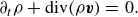 \begin{align} \partial _t \rho + \textrm{div}(\rho \boldsymbol{v}) &=\,0. \end{align}
 \begin{align} \partial _t \phi + \textrm{div}(\phi \boldsymbol{v}) - \textrm{div} \left ( \breve {\boldsymbol{M}} \nabla \left (\breve {\mu }+\omega \lambda \right )\right ) +\breve {m} \left (\breve {\mu }+\omega \breve {\lambda }\right ) &=\,0. \end{align}
Here $\phi$
is the phase-field quantity defined as the difference between volume fractions:
$\phi$
is the phase-field quantity defined as the difference between volume fractions:
 \begin{align} \phi = \phi _1 - \phi _2, \end{align}
where we recall $\phi _1+\phi _2=1$
. The chemical potential quantity is defined as
$\phi _1+\phi _2=1$
. The chemical potential quantity is defined as
 \begin{align} \breve {\mu } = \frac {\partial \Psi }{\partial \phi } - \textrm{div}\frac {\partial \Psi }{\partial \nabla \phi }. \end{align}
Finally, the quantity $\omega$
is
$\omega$
is $\omega = (\rho _1^{-1}-\rho _2^{-1})/(\rho _1^{-1}+\rho _2^{-1})$
. On the other hand, the model (4.7) takes for binary mixtures the following form (where we directly enforce
$\omega = (\rho _1^{-1}-\rho _2^{-1})/(\rho _1^{-1}+\rho _2^{-1})$
. On the other hand, the model (4.7) takes for binary mixtures the following form (where we directly enforce $\phi _1+\phi _2=1$
):
$\phi _1+\phi _2=1$
):
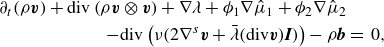 \begin{align} \partial _t (\rho \boldsymbol{v}) + \textrm{div} \left ( \rho \boldsymbol{v}\otimes \boldsymbol{v} \right ) + \nabla \lambda + \phi _1\nabla \hat {\mu }_1 + \phi _2\nabla \hat {\mu }_2 &\nonumber \\ - \textrm{div} \left ( \nu (2\nabla ^s \boldsymbol{v}+\bar {\lambda }(\textrm{div}\boldsymbol{v}) \boldsymbol{I}) \right )-\rho \boldsymbol{b} &=\, 0, \end{align}
 \begin{align} \partial _t \phi _1 + \textrm{div}(\phi _1 \boldsymbol{v}) - \rho _1^{-1}\textrm{div} \left ( \boldsymbol{M} \nabla \left (g_1 -g_2\right )\right ) +\rho _1^{-1}m \left (g_1 -g_2\right ) &=\,0, \end{align}
 \begin{align} \partial _t \phi _2 + \textrm{div}(\phi _2 \boldsymbol{v}) - \rho _2^{-1}\textrm{div} \left ( \boldsymbol{M} \nabla \left (g_2 -g_1\right )\right ) +\rho _2^{-1} m \left (g_2 -g_1\right ) &=\,0, \end{align}
where $\boldsymbol{M} = \boldsymbol{M}_{12}=\boldsymbol{M}_{21}$
and
$\boldsymbol{M} = \boldsymbol{M}_{12}=\boldsymbol{M}_{21}$
and $m=m_{12}=m_{21}$
. By means of variable transformation, we aim to express the model in terms of the quantities of model (5.1). The mass balance equations (5.4b
) and (5.4c
) can be written as
$m=m_{12}=m_{21}$
. By means of variable transformation, we aim to express the model in terms of the quantities of model (5.1). The mass balance equations (5.4b
) and (5.4c
) can be written as
 \begin{align} \partial _t \phi \!+\! \textrm{div}(\phi \boldsymbol{v}) - \textrm{div} \left ( (\rho _1^{-1}\!+\!\rho _2^{-1})\boldsymbol{M} \nabla \left (g_1 -g_2\right )\right ) \!+\! (\rho _1^{-1}+\rho _2^{-1})m \left (g_1 -g_2\right ) &=0, \end{align}
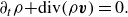 \begin{align} \partial _t \rho \!+\! \textrm{div}(\rho \boldsymbol{v}) &=0. \end{align}
With the aim of comparing the two models, we select the relations $\breve {\boldsymbol{M}}=(\rho _1^{-1}+\rho _2^{-1})^2\boldsymbol{M}$
and
$\breve {\boldsymbol{M}}=(\rho _1^{-1}+\rho _2^{-1})^2\boldsymbol{M}$
and $\breve {m}=(\rho _1^{-1}+\rho _2^{-1})^2m$
, which converts (5.5a
) into
$\breve {m}=(\rho _1^{-1}+\rho _2^{-1})^2m$
, which converts (5.5a
) into
 \begin{align} \partial _t \phi + \textrm{div}(\phi \boldsymbol{v}) - \textrm{div} \left ( \breve {\boldsymbol{M}} \nabla \left (\grave {\mu } +\omega \lambda \right )\right ) +\breve {m} \left (\grave {\mu }+\omega \lambda \right ) &=\,0, \end{align}
with $\grave {\mu } = (\rho _1^{-1}+\rho _2^{-1})^{-1}(\rho _1^{-1}\mu _1-\rho _2^{-1}\mu _2)$
. As a consequence, in case the identities
$\grave {\mu } = (\rho _1^{-1}+\rho _2^{-1})^{-1}(\rho _1^{-1}\mu _1-\rho _2^{-1}\mu _2)$
. As a consequence, in case the identities
 \begin{align} \phi _1 \nabla \hat {\mu }_1 + \phi _2 \nabla \hat {\mu }_2 =&\, \phi \nabla \breve {\mu }, \end{align}
 \begin{align} \grave {\mu } =&\,\breve {\mu }, \end{align}
hold, we find that (5.4) coincides with (5.1). This is in general not the case, i.e. in general the two models do not match. (An $N$
-phase theory that reduces to existing two-phase models emerges when working with
$N$
-phase theory that reduces to existing two-phase models emerges when working with $N-1$
order parameters
$N-1$
order parameters $\phi _\alpha$
, rather than the current case of
$\phi _\alpha$
, rather than the current case of $N$
order parameters
$N$
order parameters $\phi _\alpha$
.) There are, however, specific situations in which the models coincide, for instance when
$\phi _\alpha$
.) There are, however, specific situations in which the models coincide, for instance when $\mu _1 + \mu _2 = 0$
and
$\mu _1 + \mu _2 = 0$
and $\breve {\mu } = \mu _1 = -\mu _2$
. These conditions are inspired by the chain rule for chemical potentials, where
$\breve {\mu } = \mu _1 = -\mu _2$
. These conditions are inspired by the chain rule for chemical potentials, where $\phi =\phi (\phi _1,\phi _2)=\phi _1-\phi _2$
so that
$\phi =\phi (\phi _1,\phi _2)=\phi _1-\phi _2$
so that $\partial \phi /\partial \phi _1 = 1$
,
$\partial \phi /\partial \phi _1 = 1$
, $\partial \phi /\partial \phi _2 = -1$
of (5.2).
$\partial \phi /\partial \phi _2 = -1$
of (5.2).
5.2. $N$
-phase model Dong (Reference Dong2018)
$N$
-phase model Dong (Reference Dong2018)

The $N$
-phase incompressible model proposed by Dong (Reference Dong2018) is given by
$N$
-phase incompressible model proposed by Dong (Reference Dong2018) is given by
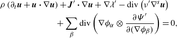 \begin{align} \rho \left (\partial _t \boldsymbol{u} + \boldsymbol{u}\,{\boldsymbol\cdot}\, \nabla \boldsymbol{u} \right ) + \boldsymbol{J}' \,{\boldsymbol\cdot}\, \nabla \boldsymbol{u} + \nabla \lambda ' - \textrm{div}\left ( \nu ' \nabla ^s \boldsymbol{u} \right ) &\nonumber \\ + \sum _{\beta } \textrm{div}\left (\nabla \phi _\alpha \otimes \frac {\partial \Psi '}{\partial (\nabla \phi _{\beta })}\right ) =&\,0, \end{align}
 \begin{align} \textrm{div}\boldsymbol{u} =&\,0, \end{align}
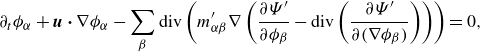 \begin{align} \partial _t \phi _\alpha + \boldsymbol{u}\,{\boldsymbol\cdot}\, \nabla \phi _\alpha - \sum _{\beta } \textrm{div}\left ( m_{\alpha {\beta }}' \nabla \left ( \frac {\partial \Psi '}{\partial \phi _{\beta }} - \textrm{div}\left (\frac {\partial \Psi '}{\partial (\nabla \phi _{\beta })}\right )\right ) \right ) =&\,0, \end{align}
for $\alpha = 1,\ldots , N$
, where
$\alpha = 1,\ldots , N$
, where $\lambda '$
is the Lagrange multiplier pressure,
$\lambda '$
is the Lagrange multiplier pressure, $\nu '$
is the dynamic viscosity,
$\nu '$
is the dynamic viscosity, $\Psi '$
is the free energy,
$\Psi '$
is the free energy, $\boldsymbol{J}'$
is the peculiar velocity, and
$\boldsymbol{J}'$
is the peculiar velocity, and $m_{\alpha {\beta }}'$
is the mobility. For the purpose of comparing the model (5.8) to the proposed framework, we define the chemical potential:
$m_{\alpha {\beta }}'$
is the mobility. For the purpose of comparing the model (5.8) to the proposed framework, we define the chemical potential:
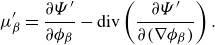 \begin{align} \mu _{\beta }' = \frac {\partial \Psi '}{\partial \phi _{\beta }} - \textrm{div}\left (\frac {\partial \Psi '}{\partial (\nabla \phi _{\beta })}\right ). \end{align}
Invoking Lemma4.1, we rewrite the model (5.8) as
 \begin{align} \rho \left (\partial _t \boldsymbol{u} + \boldsymbol{u}{\boldsymbol\cdot} \nabla \boldsymbol{u} \right ) + \boldsymbol{J}'{\boldsymbol\cdot} \nabla \boldsymbol{u} + \nabla \tilde {\lambda }' + \sum _{\beta } \phi _\alpha \nabla \mu _\alpha ' - \textrm{div}\left ( \nu ' \nabla ^s \boldsymbol{u} \right ) =&\,0, \end{align}
 \begin{align} \textrm{div}\boldsymbol{u} =&\,0, \end{align}
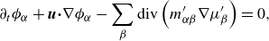 \begin{align} \partial _t \phi _\alpha + \boldsymbol{u}{\boldsymbol\cdot} \nabla \phi _\alpha - \sum _{\beta } \textrm{div}\left ( m_{\alpha {\beta }}' \nabla \mu _{\beta }' \right ) =&\,0, \end{align}
with
 \begin{align} \tilde {\lambda }' = \lambda ' + \Psi ' - \sum _{\beta } \phi _\alpha \mu _\alpha '. \end{align}
This model (5.10) is not compatible with the framework proposed in the current paper. In particular, comparing (5.10) with (4.11), we observe the following.
-
(i) Model (5.10) does not contain each of the peculiar velocity terms in the momentum equation; this applies to both inertia and viscous terms.
-
(ii) Model (5.10) does not include mass transfer terms.
-
(iii) The constitutive model for the diffusive flux in (5.10) is different; in particular the Lagrange multiplier is absent. As a consequence, the equilibrium conditions are different.
5.3. Class-II mixture model
We compare the proposed unified modelling framework with an incompressible mixture model presented in ten Eikelder et al. (Reference ten Eikelder, van der Zee and Schillinger2024):
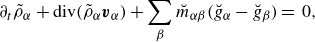 \begin{align} \partial _t \tilde {\rho }_\alpha + \textrm{div}(\tilde {\rho }_\alpha \boldsymbol{v}_\alpha ) + \sum _{\beta } \breve {m}_{\alpha {\beta }}(\breve {g}_\alpha -\breve {g}_{\beta }) &=\, 0, \end{align}
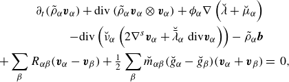 \begin{align} \partial _t (\tilde {\rho }_\alpha \boldsymbol{v}_\alpha ) + \textrm{div} \left ( \tilde {\rho }_\alpha \boldsymbol{v}_\alpha \otimes \boldsymbol{v}_\alpha \right ) + \phi _\alpha \nabla \left (\breve {\lambda } + \breve {\mu }_\alpha \right ) \nonumber \\ - \textrm{div}\left (\breve {\nu }_\alpha \left (2\nabla ^s \boldsymbol{v}_\alpha + \breve {\bar {\lambda }}_\alpha \textrm{ div}\boldsymbol{v}_\alpha \right )\right ) -\tilde {\rho }_\alpha \boldsymbol{b}&\nonumber \\ +\displaystyle \sum _{{\beta }} R_{\alpha {\beta }} (\boldsymbol{v}_\alpha -\boldsymbol{v}_{\beta }) + \tfrac {1}{2}\sum _{\beta } \breve {m}_{\alpha {\beta }}(\breve {g}_\alpha -\breve {g}_{\beta })(\boldsymbol{v}_\alpha +\boldsymbol{v}_{\beta }) &=\, 0, \end{align}
for constituents $\alpha = 1,\ldots ,N$
. Here
$\alpha = 1,\ldots ,N$
. Here $\boldsymbol{v}_\alpha$
is the constituent velocity,
$\boldsymbol{v}_\alpha$
is the constituent velocity, $\breve {\lambda }$
is a Lagrange multiplier,
$\breve {\lambda }$
is a Lagrange multiplier, $\tilde {\nu }_\alpha$
the constituent dynamical viscosity,
$\tilde {\nu }_\alpha$
the constituent dynamical viscosity, $\breve {\bar {\lambda }}_\alpha \geqslant 2/d$
,
$\breve {\bar {\lambda }}_\alpha \geqslant 2/d$
, $\nabla ^s \boldsymbol{v}_\alpha$
the constituent symmetric velocity gradient, and
$\nabla ^s \boldsymbol{v}_\alpha$
the constituent symmetric velocity gradient, and $\breve {m}_{\alpha {\beta }}$
and
$\breve {m}_{\alpha {\beta }}$
and $R_{\alpha {\beta }}$
are symmetric matrices (for the properties see ten Eikelder et al. Reference ten Eikelder, van der Zee and Schillinger2024). This model considers the free energy class:
$R_{\alpha {\beta }}$
are symmetric matrices (for the properties see ten Eikelder et al. Reference ten Eikelder, van der Zee and Schillinger2024). This model considers the free energy class:
 \begin{align} \Psi =&\, \sum _\alpha \breve {\Psi }_\alpha , \end{align}
 \begin{align} \breve {\Psi }_\alpha =&\, \breve {\Psi }_\alpha \left (\phi _\alpha , \nabla \phi _\alpha \right ). \end{align}
The associated constituent chemical potentials are defined as
 \begin{align} \breve {\mu }_\alpha =&\, \frac { \partial \breve {\Psi }_\alpha }{\partial \phi _\alpha } - \textrm{div}\frac {\partial \breve {\Psi }_\alpha }{\partial \nabla \phi _\alpha }, \end{align}
and $\breve {g}_\alpha = \rho _\alpha ^{-1}(\breve {\mu }_\alpha + \breve {\lambda })$
.
$\breve {g}_\alpha = \rho _\alpha ^{-1}(\breve {\mu }_\alpha + \breve {\lambda })$
.
Inserting the class (5.13) into the proposed modelling framework, we find $\breve {\mu }_\alpha =\hat {\mu }_\alpha$
. Additionally, we identify
$\breve {\mu }_\alpha =\hat {\mu }_\alpha$
. Additionally, we identify $\breve {\lambda }=\lambda$
; consequently
$\breve {\lambda }=\lambda$
; consequently $\breve {g}_\alpha =g_\alpha$
. In contrast to the unified modelling framework presented in the current paper, this model comprises
$\breve {g}_\alpha =g_\alpha$
. In contrast to the unified modelling framework presented in the current paper, this model comprises $N$
mass balance equations, and
$N$
mass balance equations, and $N$
momentum balance equations. As such, we compare the
$N$
momentum balance equations. As such, we compare the $N$
mass balance laws, and the single mixture momentum balance law of the models. Starting with the mass balance laws, (5.12a
) can be written as
$N$
mass balance laws, and the single mixture momentum balance law of the models. Starting with the mass balance laws, (5.12a
) can be written as
 \begin{align} \partial _t \phi _\alpha + \textrm{div}(\phi _\alpha \boldsymbol{v}) + \rho _\alpha ^{-1}\textrm{div}\boldsymbol{J}_\alpha + \rho _\alpha ^{-1}\breve {\gamma }_\alpha &=\, 0, \end{align}
 \begin{align} \breve {\gamma }_\alpha - \sum _{\beta } \breve {m}_{\alpha {\beta }}(\breve {g}_\alpha -\breve {g}_{\beta })&=\,0. \end{align}
This form is very similar to (4.7b
); the key difference is that the peculiar velocity $\boldsymbol{J}_\alpha$
is governed by a constitutive model
$\boldsymbol{J}_\alpha$
is governed by a constitutive model $\boldsymbol{J}_\alpha = \hat {\boldsymbol{J}}_\alpha$
in the current paper, whereas in (5.12) it follows from the constitutive velocities. With the identification
$\boldsymbol{J}_\alpha = \hat {\boldsymbol{J}}_\alpha$
in the current paper, whereas in (5.12) it follows from the constitutive velocities. With the identification $m_{\alpha {\beta }} = - \breve {m}_{\alpha {\beta }}$
for
$m_{\alpha {\beta }} = - \breve {m}_{\alpha {\beta }}$
for $\alpha \neq {\beta }$
and
$\alpha \neq {\beta }$
and $m_{\alpha {\beta }} = \sum _{{\gamma }\neq \alpha } \breve {m}_{\alpha {\gamma }}$
for
$m_{\alpha {\beta }} = \sum _{{\gamma }\neq \alpha } \breve {m}_{\alpha {\gamma }}$
for $\alpha = {\beta }$
(similar to Remark3.16) the mass transfer terms match (except for the difference
$\alpha = {\beta }$
(similar to Remark3.16) the mass transfer terms match (except for the difference $\hat {\boldsymbol{j}}_\alpha =0$
in (4.7b
)). Focusing on the momentum balance laws, addition of (5.12b
) provides
$\hat {\boldsymbol{j}}_\alpha =0$
in (4.7b
)). Focusing on the momentum balance laws, addition of (5.12b
) provides
 \begin{align} \partial _t (\rho \boldsymbol{v}) + \textrm{div} \left ( \rho \boldsymbol{v}\otimes \boldsymbol{v} \right ) + \sum \phi _\alpha \nabla \left (\breve {\lambda } + \breve {\mu }_\alpha \right )& \nonumber \\ - \textrm{div}\left (\sum _\alpha \breve {\nu }_\alpha \left (2\nabla ^s \boldsymbol{v} + \breve {\bar {\lambda }}_\alpha \textrm{div}\boldsymbol{v}\right )\right ) -\rho \boldsymbol{b}&\nonumber \\ - \textrm{div}\left (\sum _\alpha \breve {\nu }_\alpha \left (2\nabla ^s \boldsymbol{w}_\alpha + \breve {\bar {\lambda }}_\alpha \textrm{ div}\boldsymbol{w}_\alpha \right )- \sum _\alpha \tilde {\rho }_\alpha \boldsymbol{w}_\alpha \otimes \boldsymbol{w}_\alpha \right )&\,=0, \end{align}
where we have adopted the identities
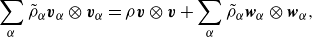 \begin{align} \sum _\alpha \tilde {\rho }_\alpha \boldsymbol{v}_\alpha \otimes \boldsymbol{v}_\alpha =&\, \rho \boldsymbol{v} \otimes \boldsymbol{v} + \sum _\alpha \tilde {\rho }_\alpha \boldsymbol{w}_\alpha \otimes \boldsymbol{w}_\alpha , \end{align}
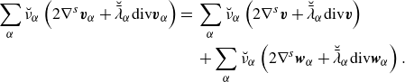 \begin{align} \sum _\alpha \breve {\nu }_\alpha \left (2\nabla ^s \boldsymbol{v}_\alpha + \breve {\bar {\lambda }}_\alpha \textrm{div}\boldsymbol{v}_\alpha \right ) =&\, \sum _\alpha \breve {\nu }_\alpha \left (2\nabla ^s \boldsymbol{v} + \breve {\bar {\lambda }}_\alpha \textrm{div}\boldsymbol{v}\right ) \nonumber \\ &\,+ \sum _\alpha \breve {\nu }_\alpha \left (2\nabla ^s \boldsymbol{w}_\alpha + \breve {\bar {\lambda }}_\alpha \textrm{div}\boldsymbol{w}_\alpha \right ). \end{align}
With the identifications $\nu = \sum _\alpha \breve {\nu }_\alpha$
and
$\nu = \sum _\alpha \breve {\nu }_\alpha$
and $\bar {\lambda }=\breve {\bar {\lambda }}_\alpha$
, the first two lines match the momentum equation (4.7a
). The last line in (5.16) consists of terms that are absent in (4.7a
). This is a direct consequence of energy-dissipation law (3.3) and the introduction of the model
$\bar {\lambda }=\breve {\bar {\lambda }}_\alpha$
, the first two lines match the momentum equation (4.7a
). The last line in (5.16) consists of terms that are absent in (4.7a
). This is a direct consequence of energy-dissipation law (3.3) and the introduction of the model $\boldsymbol{J}_\alpha =\hat {\boldsymbol{J}}_\alpha$
in (3.30b
). In the case of matching constitutive velocities, as described in § 4.2, these terms vanish.
$\boldsymbol{J}_\alpha =\hat {\boldsymbol{J}}_\alpha$
in (3.30b
). In the case of matching constitutive velocities, as described in § 4.2, these terms vanish.
6. Conclusion and outlook
This paper presents a unified framework for $N$
-phase Navier–Stokes Cahn–Hilliard Allen–Cahn mixture models with non-matching densities. The framework finds its roots in continuum mixture theory, which serves as a fundamental guiding principle for designing multiphysics models at large. The unified framework proposes a (phase-field) system of
$N$
-phase Navier–Stokes Cahn–Hilliard Allen–Cahn mixture models with non-matching densities. The framework finds its roots in continuum mixture theory, which serves as a fundamental guiding principle for designing multiphysics models at large. The unified framework proposes a (phase-field) system of $N$
mass balance laws, and one momentum balance law, that is invariant to the set of fundamental variables, has an energy-dissipative structure, is reduction-consistent, symmetric with respect to the numbering of the phases, and provides well-defined equilibrium solutions. More specifically, we draw the following conclusions.
$N$
mass balance laws, and one momentum balance law, that is invariant to the set of fundamental variables, has an energy-dissipative structure, is reduction-consistent, symmetric with respect to the numbering of the phases, and provides well-defined equilibrium solutions. More specifically, we draw the following conclusions.
-
(i) The form of the balance laws is invariant to the set of fundamental variables, at both the constituent and mixture levels (§ 2.2 and § 2.3).
-
(ii) The free energy class depends on all volume fractions (and their gradients) (§ 3.1 and § 3.2); this provides symmetry with respect to the numbering of the constituents.
-
(iii) Chemical potentials are tightly connected to the Lagrange multiplier that enforces volume conservation; these quantities occur only as superposition (§ 3.2).
-
(iv) The unified framework is invariant to the set of independent variables, both before and after constitutive modelling (§ 3.3 and § 3.4).
-
(v) Constitutive quantities are such that the resulting model exhibits energy dissipation (§ 3.4).
-
(vi) Consistency with the single-phase equations requires mobility quantities to be degenerate (§ 3.4).
-
(vii) Equilibrium solutions are determined by a balance of (generalised) chemical potentials (see § 4.3).
-
(viii) In the binary case, the framework does, in general, not coincide with existing two-phase models (see § 5.1). Furthermore, the framework is closely connected to a class-II model (see § 5.3), and the model of Dong (Reference Dong2018) does not fit into the framework (see § 5.2).
While the proposed unified framework offers insight into the modelling of $N$
-phase flows, we do not claim that it is complete. Therefore, we delineate potential future research directions. First, it is important to study the implications of the particular form of the free energy model, such as equilibrium characteristics, and Ostwald ripening phenomena (see e.g. ten Eikelder & Khanwale Reference ten Eikelder and Khanwale2024). To this purpose, we acknowledge the existence of numerous
$N$
-phase flows, we do not claim that it is complete. Therefore, we delineate potential future research directions. First, it is important to study the implications of the particular form of the free energy model, such as equilibrium characteristics, and Ostwald ripening phenomena (see e.g. ten Eikelder & Khanwale Reference ten Eikelder and Khanwale2024). To this purpose, we acknowledge the existence of numerous $N$
-phase free energy closure models (see e.g. Boyer & Minjeaud Reference Boyer and Minjeaud2014). Second, it is essential to investigate the sharp interface asymptotic behaviour (e.g. jump conditions at interfaces) for particular closure models. The last point concerns the design of (property-preserving) numerical schemes. Details of
$N$
-phase free energy closure models (see e.g. Boyer & Minjeaud Reference Boyer and Minjeaud2014). Second, it is essential to investigate the sharp interface asymptotic behaviour (e.g. jump conditions at interfaces) for particular closure models. The last point concerns the design of (property-preserving) numerical schemes. Details of $N$
-phase computations will be presented elsewhere; however, we provide some considerations here. First, a numerical simulation requires specification of the free energy (as mentioned earlier). It is hereby important to take (4.3) into account to ensure applicability to a general number of constituents. A second consideration concerns the choice of fundamental variables. Although the framework remains invariant to the choice of variables (e.g. using a mass-averaged (1.1) or volume-averaged velocity (1.2)), certain selections may be more advantageous for designing property-preserving numerical methods. Next, although the proposed system is fully symmetric with respect to the set of variables, in the numerical solution there are at least two roads one can pursue: (i) work with the full set of volume fractions and enforce the saturation constraint with a Lagrange multiplier (as detailed here), (ii) work with
$N$
-phase computations will be presented elsewhere; however, we provide some considerations here. First, a numerical simulation requires specification of the free energy (as mentioned earlier). It is hereby important to take (4.3) into account to ensure applicability to a general number of constituents. A second consideration concerns the choice of fundamental variables. Although the framework remains invariant to the choice of variables (e.g. using a mass-averaged (1.1) or volume-averaged velocity (1.2)), certain selections may be more advantageous for designing property-preserving numerical methods. Next, although the proposed system is fully symmetric with respect to the set of variables, in the numerical solution there are at least two roads one can pursue: (i) work with the full set of volume fractions and enforce the saturation constraint with a Lagrange multiplier (as detailed here), (ii) work with $N-1$
volume fractions and compute the
$N-1$
volume fractions and compute the $N$
th volume fraction from the others. In the second case, the system of equations becomes
$N$
th volume fraction from the others. In the second case, the system of equations becomes
 \begin{align} \partial _t (\rho \boldsymbol{v}) \!+\! \textrm{div} \left ( \rho \boldsymbol{v}\otimes \boldsymbol{v} \right ) \!+\! \sum _{\beta } \phi _{\beta } \nabla \mu _{\beta } \!+\! \nabla \lambda - \textrm{div} \left ( \nu (2 \nabla ^s \boldsymbol{v}\!+\!\bar {\lambda }(\textrm{div}\boldsymbol{v}) \boldsymbol{I}) \right )-\rho \boldsymbol{b} &= 0, \end{align}
 \begin{align} \partial _t \phi _\alpha + \textrm{div}(\phi _\alpha \boldsymbol{v}) +\rho _\alpha ^{-1}\textrm{div} (\hat {\boldsymbol{H}}_\alpha ) -\rho _\alpha ^{-1} \hat {\zeta }_\alpha &=0, \end{align}
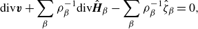 \begin{align} \textrm{div}\boldsymbol{v} + \displaystyle \sum _{{\beta }} \rho _{\beta }^{-1} \textrm{div} \hat {\boldsymbol{H}}_{\beta } - \displaystyle \sum _{{\beta }}\rho _{\beta }^{-1}\hat {\zeta }_{\beta } &= 0, \end{align}
for $\alpha \neq \gamma$
for some fixed
$\alpha \neq \gamma$
for some fixed $\gamma$
, with
$\gamma$
, with $\hat {\boldsymbol{H}}_\alpha =- \sum _{\beta } \boldsymbol{B}_{\alpha {\beta }}\nabla g_{\beta }$
,
$\hat {\boldsymbol{H}}_\alpha =- \sum _{\beta } \boldsymbol{B}_{\alpha {\beta }}\nabla g_{\beta }$
, $\hat {\zeta }_\alpha =- \sum _{\beta } m_{\alpha {\beta }} g_{\beta }$
, where the mass-averaged velocity is adopted. When working with the mass-averaged velocity, the terms
$\hat {\zeta }_\alpha =- \sum _{\beta } m_{\alpha {\beta }} g_{\beta }$
, where the mass-averaged velocity is adopted. When working with the mass-averaged velocity, the terms $\hat {\boldsymbol{H}}_\alpha = \hat {\boldsymbol{J}}_\alpha + \hat {\boldsymbol{j}}_\alpha$
may be modelled together rather than determining
$\hat {\boldsymbol{H}}_\alpha = \hat {\boldsymbol{J}}_\alpha + \hat {\boldsymbol{j}}_\alpha$
may be modelled together rather than determining $\hat {\boldsymbol{J}}_\alpha$
and
$\hat {\boldsymbol{J}}_\alpha$
and $\hat {\boldsymbol{j}}_\alpha$
independently. In contrast, within the volume-averaged velocity formulation of the model, these terms serve a distinct role. Taking
$\hat {\boldsymbol{j}}_\alpha$
independently. In contrast, within the volume-averaged velocity formulation of the model, these terms serve a distinct role. Taking $\boldsymbol{j}_\alpha = 0$
and
$\boldsymbol{j}_\alpha = 0$
and $\zeta _\alpha = 0$
,
$\zeta _\alpha = 0$
, $\alpha = 1,\ldots ,N$
then provides a divergence-free velocity. Finally, the model can accommodate large differences in specific densities between constituents. Ensuring this property in the fully discrete case requires a robust numerical method.
$\alpha = 1,\ldots ,N$
then provides a divergence-free velocity. Finally, the model can accommodate large differences in specific densities between constituents. Ensuring this property in the fully discrete case requires a robust numerical method.
Declaration of interests
The author reports no conflict of interest.
Appendix A. Reduced free energy class and proofs
We briefly discuss the free energy class with reduced dependency:
 \begin{align} \Psi =&\, {\hat {\hat {\Psi }}}^{(\beta )}\left (\left \{\phi _\alpha \right \}_{\alpha \neq {\beta }},\left \{\nabla \phi _\alpha \right \}_{\alpha \neq {\beta }}\right ), \end{align}
where the constituent number $\beta \in \{1,\ldots ,N\}$
is fixed, and where both
$\beta \in \{1,\ldots ,N\}$
is fixed, and where both $\left \{\phi _\alpha \right \}_{\alpha \neq {\beta }}$
and
$\left \{\phi _\alpha \right \}_{\alpha \neq {\beta }}$
and $\left \{\nabla \phi _\alpha \right \}_{\alpha \neq {\beta }}$
consist of independent variables. The class (A1) is connected to (3.5) via the identification
$\left \{\nabla \phi _\alpha \right \}_{\alpha \neq {\beta }}$
consist of independent variables. The class (A1) is connected to (3.5) via the identification
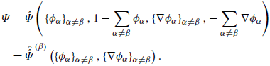
The associated chemical potentials take the form
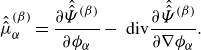 \begin{align} {\hat {\hat {\mu }}}_\alpha^{(\beta )} = \frac { \partial {\hat{\hat{\Psi}}}{}^{(\beta )}}{\partial \phi _\alpha } - \textrm{ div}\frac {\partial {\hat {\hat {\Psi }}}{}^{(\beta )}}{\partial \nabla \phi _\alpha }. \end{align}
Lemma A.1 (Chemical potentials reduced class). The chemical potentials of the reduced class may be expressed as
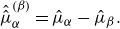 \begin{align} {\hat {\hat {\mu }}}_\alpha ^{(\beta )} = \hat {\mu }_\alpha - \hat {\mu }_{\beta }. \end{align}
Proof. Direct evaluation of the partial derivatives provides
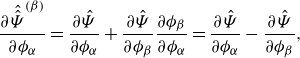 \begin{align} \frac {\partial {\hat {\hat {\Psi }}}^{(\beta )}}{\partial \phi _\alpha } =&\, \frac {\partial \hat {\Psi }}{\partial \phi _\alpha }+\frac {\partial \hat {\Psi }}{\partial \phi _{\beta }}\frac {\partial \phi _{\beta }}{\partial \phi _\alpha } = \frac {\partial \hat {\Psi }}{\partial \phi _\alpha }-\frac {\partial \hat {\Psi }}{\partial \phi _{\beta }}, \end{align}
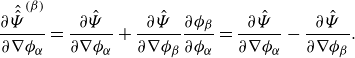 \begin{align} \frac {\partial {\hat {\hat {\Psi }}}^{(\beta )}}{\partial \nabla \phi _\alpha } = &\,\frac {\partial \hat {\Psi }}{\partial \nabla \phi _\alpha }+\frac {\partial \hat {\Psi }}{\partial \nabla \phi _{\beta }}\frac {\partial \phi _{\beta }}{\partial \phi _\alpha } = \frac {\partial \hat {\Psi }}{\partial \nabla \phi _\alpha }-\frac {\partial \hat {\Psi }}{\partial \nabla \phi _{\beta }}. \end{align}
The linearity of the divergence operator concludes the proof.
Lemma A.2 (Derivative of the free energy). The derivative of the free energy class (3.5) , i.e.
 \begin{align} \textrm{d}\hat {\Psi } = \sum _{\alpha } \frac {\partial \hat {\Psi }}{\partial \phi _\alpha } \textrm{d}\phi _\alpha + \sum _{\alpha } \frac {\partial \hat {\Psi }}{\partial \nabla \phi _\alpha } \textrm{d}(\nabla \phi _\alpha ), \end{align}
is not altered by enforcing the summation constraint (2.5b), where $\textrm{d}$
is the derivative operator.
$\textrm{d}$
is the derivative operator.
Proof.
Inserting (A5), the derivative of $\Psi$
takes the form
$\Psi$
takes the form
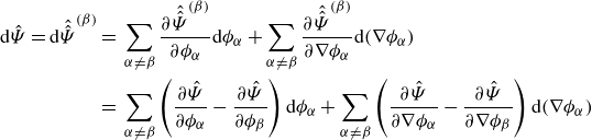 \begin{align*} \textrm{d}\hat {\Psi } =\textrm{d} {\hat {\hat {\Psi }}}^{(\beta )} =&\, \sum _{\alpha \neq {\beta }} \frac {\partial {\hat {\hat {\Psi }}}^{(\beta )}}{\partial \phi _\alpha } \textrm{d}\phi _\alpha + \sum _{\alpha \neq {\beta }} \frac {\partial {\hat {\hat {\Psi }}}^{(\beta )}}{\partial \nabla \phi _\alpha } \textrm{d}(\nabla \phi _\alpha )\nonumber \\=&\, \sum _{\alpha \neq {\beta }} \left (\frac {\partial \hat {\Psi }}{\partial \phi _\alpha }-\frac {\partial \hat {\Psi }}{\partial \phi _{\beta }}\right ) \textrm{d}\phi _\alpha + \sum _{\alpha \neq {\beta }} \left (\frac {\partial \hat {\Psi }}{\partial \nabla \phi _\alpha }-\frac {\partial \hat {\Psi }}{\partial \nabla \phi _{\beta }}\right ) \textrm{d}(\nabla \phi _\alpha ) \end{align*}
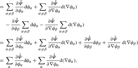 \begin{align} =&\, \sum _{\alpha \neq {\beta }} \frac {\partial \hat {\Psi }}{\partial \phi _\alpha } \textrm{d}\phi _\alpha + \sum _{\alpha \neq {\beta }} \frac {\partial \hat {\Psi }}{\partial \nabla \phi _\alpha } \textrm{d}(\nabla \phi _\alpha ) \nonumber \\ &\,- \frac {\partial \hat {\Psi }}{\partial \phi _{\beta }}\sum _{\alpha \neq {\beta }} \textrm{d}\phi _\alpha - \frac {\partial \hat {\Psi }}{\partial \nabla \phi _{\beta }}\sum _{\alpha \neq {\beta }} \textrm{d}(\nabla \phi _\alpha )\nonumber \\ =&\, \sum _{\alpha \neq {\beta }} \frac {\partial \hat {\Psi }}{\partial \phi _\alpha } \textrm{d}\phi _\alpha + \sum _{\alpha \neq {\beta }} \frac {\partial \hat {\Psi }}{\partial \nabla \phi _\alpha } \textrm{d}(\nabla \phi _\alpha ) + \frac {\partial \hat {\Psi }}{\partial \phi _{\beta }} \textrm{d}\phi _{\beta } + \frac {\partial \hat {\Psi }}{\partial \nabla \phi _{\beta }}\textrm{ d}(\nabla \phi _{\beta })\nonumber \\ =&\, \sum _{\alpha } \frac {\partial \hat {\Psi }}{\partial \phi _\alpha } \textrm{d}\phi _\alpha + \sum _{\alpha } \frac {\partial \hat {\Psi }}{\partial \nabla \phi _\alpha } \textrm{d}(\nabla \phi _\alpha ), \end{align}
where we have invoked $\sum _{\alpha }\textrm{d}\phi _\alpha = 0$
and
$\sum _{\alpha }\textrm{d}\phi _\alpha = 0$
and $\sum _{\alpha }\textrm{d}(\nabla \phi _\alpha ) = 0$
. The latter expression matches the unconstrained derivative.
$\sum _{\alpha }\textrm{d}(\nabla \phi _\alpha ) = 0$
. The latter expression matches the unconstrained derivative.
Lemma A.3 (Well-defined free energy terms). The following free energy terms in (3.10) are well-defined when enforcing the summation constraint (2.5b):
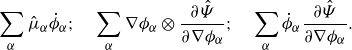 \begin{align} \sum _{\alpha } \hat {\mu }_\alpha \dot {\phi }_\alpha ; \quad \sum _{\alpha } \nabla \phi _\alpha \otimes \frac {\partial \hat {\Psi }}{\partial \nabla \phi _\alpha }; \quad \sum _{\alpha } \dot {\phi }_\alpha \frac {\partial \hat {\Psi }}{\partial \nabla \phi _\alpha }. \end{align}
Proof. We show that the first term subject to (2.5b ) is well-defined; the others follow similarly. Utilising an argumentation analogously to that of the proof of LemmaA.2, we have the following sequence of identities:
 \begin{align} \sum _{\alpha } \hat {\mu }_\alpha \dot {\phi }_\alpha =&\, \sum _{\alpha \neq {\beta }} \hat {\mu }_\alpha \dot {\phi }_\alpha + \hat {\mu }_{\beta }\dot {\phi }_{\beta }\nonumber \\ =&\,\sum _{\alpha \neq {\beta }} \hat {\mu }_\alpha \dot {\phi }_\alpha - \hat {\mu }_{\beta } \sum _{\alpha \neq {\beta }} \dot {\phi }_\alpha \nonumber \\ =&\, \sum _{\alpha \neq {\beta }} \left (\hat {\mu }_\alpha -\hat {\mu }_{\beta }\right ) \dot {\phi }_\alpha \nonumber \\ =&\,\sum _{\alpha \neq {\beta }} {\hat {\hat {\mu }}}_\alpha ^{(\beta )} \dot {\phi }_\alpha , \end{align}
where we have utilised LemmaA.1 in the last identity, where we have invoked $\sum _{\alpha }\phi _\alpha = 1$
. Since the latter expression is well-defined, so is the initial one.
$\sum _{\alpha }\phi _\alpha = 1$
. Since the latter expression is well-defined, so is the initial one.
Lemma A.4 (Free energy identity). The following identity holds:
 \begin{align} \sum _\alpha \phi _\alpha \nabla \mu _\alpha =\nabla \left (\sum _\alpha \phi _\alpha \hat {\mu }_\alpha - \hat {\Psi }\right ) + \textrm{div} \left (\sum _\alpha \nabla \phi _\alpha \otimes \frac {\partial \hat {\Psi }}{\partial \nabla \phi _\alpha } \right ). \end{align}
Proof. Expanding the derivatives of the right-hand side term yields
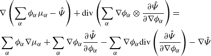 \begin{align*} &\nabla \left (\sum _\alpha \phi _\alpha \mu _\alpha - \hat {\Psi }\right ) + \textrm{div} \left (\sum _\alpha \nabla \phi _\alpha \otimes \frac {\partial \hat {\Psi }}{\partial \nabla \phi _\alpha } \right ) =\nonumber \\&\sum _\alpha \phi _\alpha \nabla \mu _\alpha +\sum _\alpha \nabla \phi _\alpha \frac { \partial \hat {\Psi }}{\partial \phi _\alpha } - \sum _\alpha \nabla \phi _\alpha \textrm{div}\left (\frac {\partial \hat {\Psi }}{\partial \nabla \phi _\alpha }\right ) - \nabla \hat {\Psi } \end{align*}
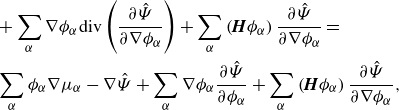 \begin{align} &+ \sum _\alpha \nabla \phi _\alpha \textrm{div} \left ( \frac {\partial \hat {\Psi }}{\partial \nabla \phi _\alpha } \right )+\sum _\alpha \left (\boldsymbol{H} \phi _\alpha \right ) \frac {\partial \hat {\Psi }}{\partial \nabla \phi _\alpha } =\nonumber \\&\sum _\alpha \phi _\alpha \nabla \mu _\alpha - \nabla \hat {\Psi } +\sum _\alpha \nabla \phi _\alpha \frac { \partial \hat {\Psi }}{\partial \phi _\alpha } +\sum _\alpha \left (\boldsymbol{H} \phi _\alpha \right ) \frac {\partial \hat {\Psi }}{\partial \nabla \phi _\alpha }, \end{align}
where $\boldsymbol{H} \phi _\alpha$
is the hessian of
$\boldsymbol{H} \phi _\alpha$
is the hessian of $\phi _\alpha$
. Observing that the sum of the latter three terms in the final expression in (A11) vanishes completes the proof.
$\phi _\alpha$
. Observing that the sum of the latter three terms in the final expression in (A11) vanishes completes the proof.
Appendix B. Equivalence of modelling restrictions
This section discusses the equivalence of the restrictions (3.21) and (3.27) via variable transformation, and some consequences of directly enforcing the saturation constraint.
First, we recall the variable transformation (2.7):
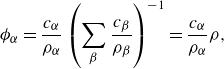 \begin{align} \phi _\alpha =&\, \frac {c_\alpha }{\rho _\alpha }\left (\sum _{\beta }\frac {c_{\beta }}{\rho _{\beta }}\right )^{-1} = \frac {c_\alpha }{\rho _\alpha }\rho , \end{align}
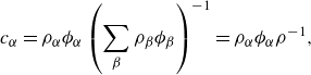 \begin{align} c_\alpha =&\, \rho _\alpha \phi _\alpha \left (\sum _{\beta }\rho _{\beta }\phi _{\beta }\right )^{-1} = \rho _\alpha \phi _\alpha \rho ^{-1}, \end{align}
where we note
 \begin{align} \rho = \hat {\rho }(\{c_{\beta }\})&\, \left (\sum _{\beta }\frac {c_{\beta }}{\rho _{\beta }}\right )^{-1}, \end{align}
 \begin{align} \rho ^{-1}=\check {\rho }^{-1}\left (\left \{\phi _{\beta }\right \}\right )&\, =\left (\sum _{\beta }\rho _{\beta }\phi _{\beta }\right )^{-1}, \end{align}
for $\alpha =1, \ldots , N$
. These variable transformations are established by directly enforcing (2.5), from which the following lemma is a consequence.
$\alpha =1, \ldots , N$
. These variable transformations are established by directly enforcing (2.5), from which the following lemma is a consequence.
Lemma B.1 (Invertibility transformation maps). The maps (B1) are not invertible.
Proof. A straightforward evaluation provides the elements of the Jacobian mappings:
 \begin{align} \frac {\partial \phi _{\beta }}{\partial c_\alpha } =&\, \rho \rho _{\beta }^{-1} \left (\delta _{\alpha {\beta }} - \rho c_{\beta } \rho _\alpha ^{-1}\right ), \end{align}
 \begin{align} \frac {\partial c_{\beta }}{\partial \phi _\alpha } =&\, \rho ^{-1} \rho _{\beta } \left (\delta _{\alpha {\beta }} - \rho ^{-1} \phi _{\beta } \rho _\alpha \right ), \end{align}
where $\delta _{\alpha {\beta }}$
is the Kronecker delta. Summation over
$\delta _{\alpha {\beta }}$
is the Kronecker delta. Summation over ${\beta } = 1,\ldots , N$
yields
${\beta } = 1,\ldots , N$
yields
 \begin{align} \sum _{\beta } \frac {\partial \phi _{\beta }}{\partial c_\alpha } = &\, 0, \end{align}
 \begin{align} \sum _{\beta } \frac {\partial c_{\beta }}{\partial \phi _\alpha } =&\, 0. \end{align}
Hence, each of the columns of the Jacobian sums to zero. Thus the columns are linearly dependent, and consequently the determinants of the both mappings vanish:
 \begin{align} \textrm{det} \frac {\partial \phi _{\beta }}{\partial c_\alpha } =&\, 0, \end{align}
 \begin{align} \textrm{det} \frac {\partial c_{\beta }}{\partial \phi _\alpha } =&\, 0.\\ \nonumber \end{align}
Next, we recall the chain rule for the chemical potential.
Lemma B.2 (Chain rule chemical potentials). We have the chain rule for chemical potentials:
 \begin{align} \check {\mu }_\alpha =&\,\sum _{\beta } \hat {\mu }_{\beta } \frac {\partial \phi _{\beta }}{\partial c_\alpha }, \end{align}
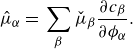 \begin{align} \hat {\mu }_\alpha =&\,\sum _{\beta } \check {\mu }_{\beta } \frac {\partial c_{\beta }}{\partial \phi _\alpha }. \end{align}
Proof. We show (B6a ) and note that (B6b ) follows similarly. A direct computation yields
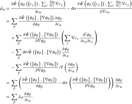 \begin{align} \check {\mu }_\alpha =&\, \frac {\partial \hat {\Psi }\left (\phi _{{\beta }}\left (\left \{c_{\gamma }\right \}\right ),\sum _{\gamma } \frac {\partial \phi _{\beta }}{\partial c_{\gamma }}\nabla c_{\gamma }\right )}{\partial c_\alpha } - \textrm{div} \frac {\partial \hat {\Psi }\left (\phi _{{\beta }}\left (\left \{c_{\gamma }\right \}\right ),\sum _{\gamma } \frac {\partial \phi _{\beta }}{\partial c_{\gamma }}\nabla c_{\gamma }\right )}{\partial \nabla c_\alpha } \nonumber \\ =&\, \sum _{\beta } \frac {\partial \hat {\Psi }\left (\left \{\phi _{{\beta }}\right \},\left \{\nabla \phi _{\beta }\right \}\right )}{\partial \phi _{\beta }}\frac {\partial \phi _{\beta }}{\partial c_\alpha }\nonumber \\ &\,+\sum _{\beta } \frac {\partial \hat {\Psi }\left (\left \{\phi _{{\beta }}\right \},\left \{\nabla \phi _{\beta }\right \}\right )}{\partial \nabla \phi _{\beta }}{\boldsymbol\cdot} \left (\sum _{\gamma } \nabla c_{\gamma }\,\frac {\partial ^2 \phi _{\beta }}{\partial c_\alpha \partial c_{\gamma }}\right )\nonumber \\ &\,-\sum _{\beta } \textrm{div} \hat {\Psi }\left (\left \{\phi _{{\beta }}\right \},\left \{\nabla \phi _{\beta }\right \}\right ) \frac {\partial \phi _{\beta }}{\partial c_\alpha } \nonumber \\ &\,-\sum _{\beta } \frac {\partial \hat {\Psi }\left (\left \{\phi _{{\beta }}\right \},\left \{\nabla \phi _{\beta }\right \}\right )}{\partial \nabla \phi _{\beta }}{\boldsymbol\cdot} \nabla \left (\frac {\partial \phi _{\beta }}{\partial c_\alpha }\right )\nonumber \\ =&\, \sum _{\beta } \left (\frac {\partial \hat {\Psi }\left (\left \{\phi _{{\beta }}\right \},\left \{\nabla \phi _{\beta }\right \}\right )}{\partial \phi _{\beta }}- \textrm{div} \left (\frac {\partial \hat {\Psi }\left (\left \{\phi _{{\beta }}\right \},\left \{\nabla \phi _{\beta }\right \}\right )}{\partial \nabla \phi _{\beta }} \right )\right ) \frac {\partial \phi _{\beta }}{\partial c_\alpha } \nonumber \\ =&\, \sum _{\beta } \hat {\mu }_{\beta } \frac {\partial \phi _{\beta }}{\partial c_\alpha }. \end{align}
Lemma B.3 (Relations between chemical quantities). The chemical potential quantities are related via the following identities:
 \begin{align} \hat {\mu }_\alpha =&\, \rho ^{-1} \rho _\alpha \left (\check {\mu }_\alpha - \sum _{\beta } \check {\mu }_{\beta } c_{\beta }\right ), \end{align}
 \begin{align} \check {\mu }_\alpha =&\, \rho \rho _\alpha ^{-1} \left (\hat {\mu }_\alpha - \sum _{\beta } \hat {\mu }_{\beta } \phi _{\beta }\right ). \end{align}
Lemma B.4 (Matching Korteweg tensors). The Korteweg stress tensors of the both modelling choices are identical:
 \begin{align} \sum _\alpha \nabla \phi _\alpha \otimes \frac {\partial \hat {\Psi }}{\partial \nabla \phi _\alpha } = \sum _\alpha \nabla c_\alpha \otimes \frac {\partial \check {\Psi }}{\partial \nabla c_\alpha }. \end{align}
Proof. This follows from (B3) and (2.5b ):
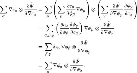 \begin{align} \sum _\alpha \nabla c_\alpha \otimes \frac {\partial \check {\Psi }}{\partial \nabla c_\alpha } =&\, \sum _\alpha \left (\sum _{\beta } \frac {\partial c_\alpha }{\partial \phi _{\beta }} \nabla \phi _{\beta }\right ) \otimes \left (\sum _{\gamma } \frac {\partial \hat {\Psi }}{\partial \nabla \phi _{\gamma }}\frac {\partial \phi _{\gamma }}{\partial c_\alpha }\right )\nonumber \\ =&\, \sum _{\alpha ,{\beta },{\gamma }} \left ( \frac {\partial c_\alpha }{\partial \phi _{\beta }} \frac {\partial \phi _{\gamma }}{\partial c_\alpha }\right ) \nabla \phi _{\beta } \otimes \frac {\partial \hat {\Psi }}{\partial \nabla \phi _{\gamma }}\nonumber \\ =&\, \sum _{{\beta },{\gamma }} \delta _{{\beta }{\gamma }} \nabla \phi _{\beta } \otimes \frac {\partial \hat {\Psi }}{\partial \nabla \phi _{\gamma }}\nonumber \\ =&\, \sum _\alpha \nabla \phi _\alpha \otimes \frac {\partial \hat {\Psi }}{\partial \nabla \phi _\alpha }. \end{align}
Theorem B.5 (Equivalence modelling restrictions). The modelling restrictions(3.21)and(3.27)are equivalent.
Proof. We select the following relations between the Lagrange multipliers of the two modelling choices:
 \begin{align} \check {\lambda }=&\, \hat {\lambda }+\sum _{\beta }\hat {\mu }_{\beta }\phi _{\beta }. \end{align}
Invoking LemmaB.4 and substituting the relation (B11) provides
 \begin{align} \check {\lambda }\boldsymbol{I} +\sum _{\alpha } \nabla c_\alpha \otimes \frac {\partial \check {\Psi }}{\partial \nabla c_\alpha } - \check {\Psi }\boldsymbol{I} = \hat {\lambda }\boldsymbol{I} +\sum _{\alpha } \nabla \phi _\alpha \otimes \frac {\partial \hat {\Psi }}{\partial \nabla \phi _\alpha } + \big(\hat {\mu }_\alpha \phi _\alpha - \check {\Psi }\big)\boldsymbol{I}. \end{align}
In a similar fashion, we find
 \begin{align} \rho ^{-1}\check {\mu }_\alpha + \rho _\alpha ^{-1}\check {\lambda } =&\, \rho _\alpha ^{-1} \Bigg (\hat {\mu }_\alpha - \sum _{\beta } \hat {\mu }_{\beta } \phi _{\beta }\Bigg ) +\rho _\alpha ^{-1}\Bigg (\hat {\lambda }+\sum _\alpha \hat {\mu }_{\beta }\phi _{\beta }\Bigg )= g_\alpha , \end{align}
and conclude
 \begin{align} - \sum _{\alpha }\nabla \left ( \rho ^{-1}\check {\mu }_\alpha + \rho _\alpha ^{-1}\check {\lambda } \right ){\boldsymbol\cdot}\ \boldsymbol{H}_\alpha =&\, - \sum _{\alpha }\nabla g_\alpha {\boldsymbol\cdot}\ \boldsymbol{H}_\alpha, \end{align}
 \begin{align} -\sum _{\alpha } \left ( \rho ^{-1}\check {\mu }_\alpha + \rho _\alpha ^{-1}\check {\lambda } \right ) \zeta _\alpha = &\,-\sum _{\alpha } g_\alpha \zeta _\alpha . \\[6pt] \nonumber \end{align}
Finally, we note that Lemma(B.1) may result in erroneous derivations. For example, from (B8) one can deduce
 \begin{align} \sum _\alpha \hat {\mu }_\alpha \phi _\alpha =&\, 0, \end{align}
 \begin{align} \sum _\alpha \check {\mu }_\alpha c_\alpha =&\, 0, \end{align}
which do not hold in general. In particular, this follows from the chain rule Lemma(B.2):
 \begin{align} \sum _\alpha \hat {\mu }_\alpha \phi _\alpha =&\, \sum _\alpha \left (\sum _{\beta } \check {\mu }_{\beta } \frac {\partial c_{\beta }}{\partial \phi _\alpha } \right )\phi _\alpha , \end{align}
 \begin{align} \sum _\alpha \check {\mu }_\alpha c_\alpha =&\,\sum _\alpha \left (\sum _{\beta } \hat {\mu }_{\beta } \frac {\partial \phi _{\beta }}{\partial c_\alpha } \right )c_\alpha , \end{align}
alongside the identities
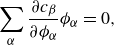 \begin{align} \sum _\alpha \frac {\partial c_{\beta }}{\partial \phi _\alpha } \phi _\alpha =&\, 0, \end{align}
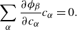 \begin{align} \sum _\alpha \frac {\partial \phi _{\beta }}{\partial c_\alpha } c_\alpha =&\, 0. \end{align}
In this situation, we have $\hat {\lambda }= \check {\lambda }$
.
$\hat {\lambda }= \check {\lambda }$
.
Appendix C. Alternative constitutive modelling
In this section, we provide some brief details on the constitutive modelling based on concentration variables. Appendix C.1 outlines the modelling assumptions, and Appendix C.2 derives the modelling restriction.
C.1. Assumptions and modelling choices
We use the balance laws (3.1), where the mass balance laws are now written in terms of concentration variables:
 \begin{align} \rho (\partial _t c_\alpha + \boldsymbol{v}{\boldsymbol\cdot} \nabla c_\alpha ) + \textrm{div} \boldsymbol{H}_\alpha &=\, \zeta _\alpha , \end{align}
 \begin{align} \partial _t (\rho \boldsymbol{v}) + \textrm{div} \left ( \rho \boldsymbol{v}\otimes \boldsymbol{v} \right ) - \textrm{div} \boldsymbol{T} - \rho \boldsymbol{b} &=\,0, \end{align}
 \begin{align} \boldsymbol{T}-\boldsymbol{T}^T &=\,0, \end{align}
where (C1a
) holds for constituents $\alpha =1,\ldots ,N$
. We use the energy-dissipation law (3.3):
$\alpha =1,\ldots ,N$
. We use the energy-dissipation law (3.3):
 \begin{align} \frac {\textrm{d}}{\textrm{d}t} \mathscr{E} = \mathscr{W} - \mathscr{D}, \end{align}
with dissipation $\mathscr{D}\geqslant 0$
and recall (3.4). We postulate the free energy to pertain to the constitutive class
$\mathscr{D}\geqslant 0$
and recall (3.4). We postulate the free energy to pertain to the constitutive class
 \begin{align} \Psi =&\, \check {\Psi }\left (\left \{c_\alpha \right \}_{\alpha =1,\ldots ,N},\left \{\nabla c_\alpha \right \}_{\alpha =1,\ldots ,N}\right ), \end{align}
subject to the summation constraint (2.5a
), and introduce the chemical potential quantities ( $\alpha = 1,\ldots ,N$
):
$\alpha = 1,\ldots ,N$
):
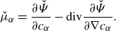 \begin{align} \check {\mu }_\alpha =&\, \frac { \partial \check {\Psi }}{\partial c_\alpha } - \textrm{div}\frac {\partial \check {\Psi }}{\partial \nabla c_\alpha }. \end{align}
C.2. Modelling restriction
By applying Reynolds transport theorem, the divergence theorem and integration by parts, and identity (3.11), the evolution of the free energy $\check {\Psi }$
takes the form
$\check {\Psi }$
takes the form
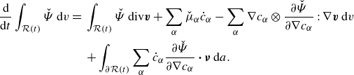 \begin{align} \frac {\textrm{d}}{\textrm{d}t}\displaystyle \int _{\mathcal{R}(t)} \check {\Psi } \,\textrm{d}v =&\, \displaystyle \int _{\mathcal{R}(t)} \check {\Psi }\,\textrm{div} \boldsymbol{v} + \sum _{\alpha } \check {\mu }_\alpha \dot {c}_\alpha - \sum _{\alpha } \nabla c_\alpha \otimes \frac {\partial \check {\Psi }}{\partial \nabla c_\alpha }: \nabla \boldsymbol{v} \,\textrm{d}v \nonumber \\ &\,+ \displaystyle \int _{\partial \mathcal{R}(t)}\sum _{\alpha } \dot {c}_\alpha \frac {\partial \check {\Psi }}{\partial \nabla c_\alpha }\,{\boldsymbol\cdot}\, \boldsymbol{\nu } \,\textrm{d}a. \end{align}
Substituting the constituent mass balance laws (3.1a ), and again applying integration by parts, yields
 \begin{align} \frac {\textrm{d}}{\textrm{d}t}\displaystyle \int _{\mathcal{R}(t)} \sum _{\alpha } \check {\Psi } \, \textrm{d}v = &\, \displaystyle \int _{\mathcal{R}(t)} \check {\Psi }\,\textrm{div} \boldsymbol{v} + \sum _{\alpha } \nabla (\rho ^{-1}\check {\mu }_\alpha )\ {\boldsymbol\cdot}\ \boldsymbol{H}_\alpha \nonumber \\ &\,\,\,- \sum _{\alpha } \nabla c_\alpha \otimes \frac {\partial \check {\Psi }}{\partial \nabla c_\alpha }: \nabla \boldsymbol{v} + \sum _{\alpha } \rho ^{-1}\check {\mu }_\alpha \zeta _\alpha \,\textrm{d}v\nonumber \\ &\,+ \displaystyle \int _{\partial \mathcal{R}(t)}\left (\sum _{\alpha } \dot {c}_\alpha \frac {\partial \check {\Psi }}{\partial \nabla c_\alpha }-\rho ^{-1}\check {\mu }_\alpha \boldsymbol{H}_\alpha \right ){\boldsymbol\cdot}\, \boldsymbol{\nu } \,\textrm{d}a. \end{align}
Addition of (3.15) and (C6) provides the evolution of the total energy:
 \begin{align} \frac {\textrm{d}}{\textrm{d}t} \mathscr{E} = &\, \displaystyle \int _{\partial \mathcal{R}(t)}\left (\boldsymbol{v}^T\boldsymbol{T}-\sum _{\alpha } \left (\rho ^{-1}\check {\mu }_\alpha \boldsymbol{H}_\alpha -\dot {c}_\alpha \frac {\partial \check {\Psi }}{\partial \nabla c_\alpha }\right )\right ){\boldsymbol\cdot}\, \boldsymbol{\nu } \,\textrm{d}a \nonumber \\ &\,- \displaystyle \int _{\mathcal{R}(t)} \left (\boldsymbol{T} +\sum _{\alpha } \nabla c_\alpha \otimes \frac {\partial \check {\Psi }}{\partial \nabla c_\alpha } - \check {\Psi }\boldsymbol{I}\right ):\nabla \boldsymbol{v}\nonumber \\ &\,\,\,\,\,\,\,\,\,\,\,+ \sum _{\alpha }\left (-\nabla (\rho ^{-1}\check {\mu }_\alpha )\ {\boldsymbol\cdot}\ \boldsymbol{H}_\alpha - \rho ^{-1}\check {\mu }_\alpha \zeta _\alpha \right )\,\textrm{d}v. \end{align}
Analogously to § 3.2, we restore the degenerate nature of (C7) via a Lagrange multiplier construction:
 \begin{align} 0=&\, \check {\lambda } \textrm{div}\boldsymbol{v} + \nabla \left (\check {\lambda } \displaystyle \sum _{\alpha } \rho _\alpha ^{-1} \boldsymbol{H}_\alpha \right ) - \sum _{\alpha } \rho _\alpha ^{-1}\boldsymbol{H}_\alpha {\boldsymbol\cdot} \nabla \check {\lambda } - \check {\lambda } \displaystyle \sum _{\alpha } \rho _\alpha ^{-1} \zeta _\alpha , \end{align}
where $\check {\lambda }$
is the scalar Lagrange multiplier. Equation (C8) follows from (2.29a
) and is impossible to derive from (C1a
) using (2.5a
). Integrating (C8) over
$\check {\lambda }$
is the scalar Lagrange multiplier. Equation (C8) follows from (2.29a
) and is impossible to derive from (C1a
) using (2.5a
). Integrating (C8) over $\mathcal{R}(t)$
and subtracting the result from (C7) provides
$\mathcal{R}(t)$
and subtracting the result from (C7) provides
 \begin{align*} \frac {\textrm{d}}{\textrm{d}t} \mathscr{E} = &\, \displaystyle \int _{\partial \mathcal{R}(t)}\left (\boldsymbol{v}^T\boldsymbol{T}-\sum _{\alpha } \left (\rho ^{-1}\check {\mu }_\alpha \boldsymbol{H}_\alpha -\dot {c}_\alpha \frac {\partial \check {\Psi }}{\partial \nabla c_\alpha }\right )-\check {\lambda } \displaystyle \sum _{\alpha } \rho _\alpha ^{-1} \boldsymbol{H}_\alpha \right ){\boldsymbol\cdot}\, \boldsymbol{\nu } \,\textrm{d}a \nonumber \\&\,- \displaystyle \int _{\mathcal{R}(t)} \left (\boldsymbol{T} + \check {\lambda }\boldsymbol{I} +\sum _{\alpha } \nabla c_\alpha \otimes \frac {\partial \check {\Psi }}{\partial \nabla c_\alpha } - \check {\Psi }\boldsymbol{I}\right ):\nabla \boldsymbol{v} \end{align*}
 \begin{align} &\,\,\,\,\,\,\,\,\,\,\,\,\,\,\,\,+ \sum _{\alpha }\left (-\nabla \left ( \rho ^{-1}\check {\mu }_\alpha + \rho _\alpha ^{-1}\check {\lambda } \right ){\boldsymbol\cdot}\ \boldsymbol{H}_\alpha \right .\nonumber \\&\,\,\,\,\,\,\,\,\,\,\,\,\,\,\,\,\,\,\,\,\,\left .- \left ( \rho ^{-1}\check {\mu }_\alpha + \rho _\alpha ^{-1}\check {\lambda } \right ) \zeta _\alpha \right )\,\textrm{d}v. \end{align}
The rate of work and the dissipation take the forms
 \begin{align} \mathscr{W} =&\, \displaystyle \int _{\partial \mathcal{R}(t)}\left (\boldsymbol{v}^T\boldsymbol{T}-\sum _{\alpha } \left (\rho ^{-1}\check {\mu }_\alpha \boldsymbol{H}_\alpha -\dot {c}_\alpha \frac {\partial \check {\Psi }}{\partial \nabla c_\alpha }\right )-\check {\lambda } \displaystyle \sum _{\alpha } \rho _\alpha ^{-1} \boldsymbol{H}_\alpha \right ){\boldsymbol\cdot}\, \boldsymbol{\nu } \,\textrm{ d}a, \end{align}
 \begin{align} \mathscr{D} =&\,\displaystyle \int _{\mathcal{R}(t)} \left (\boldsymbol{T} + \check {\lambda }\boldsymbol{I} +\sum _{\alpha } \nabla c_\alpha \otimes \frac {\partial \check {\Psi }}{\partial \nabla c_\alpha } - \check {\Psi }\boldsymbol{I}\right ):\nabla \boldsymbol{v}\nonumber \\ &\,\,\,\,\,\,\,\,\,\,\,\,\,+ \sum _{\alpha }\left (-\nabla \left ( \rho ^{-1}\check {\mu }_\alpha + \rho _\alpha ^{-1}\check {\lambda } \right ){\boldsymbol\cdot}\ \boldsymbol{H}_\alpha \right .\nonumber \\ &\,\,\,\,\,\,\,\,\,\,\,\,\,\,\,\,\,\,\, \left .-\left ( \rho ^{-1}\check {\mu }_\alpha + \rho _\alpha ^{-1}\check {\lambda } \right )\zeta _\alpha \right )\,\textrm{d}v. \end{align}
Given that the control volume $\mathcal{R}=\mathcal{R}(t)$
can be chosen arbitrarily, adhering to the energy-dissipation law requires that the following local inequality is satisfied:
$\mathcal{R}=\mathcal{R}(t)$
can be chosen arbitrarily, adhering to the energy-dissipation law requires that the following local inequality is satisfied:
 \begin{align} \left (\boldsymbol{T} + \check {\lambda }\boldsymbol{I} +\sum _{\alpha } \nabla c_\alpha \otimes \frac {\partial \check {\Psi }}{\partial \nabla c_\alpha } - \check {\Psi }\boldsymbol{I}\right ):\nabla \boldsymbol{v}&\nonumber \\ - \sum _{\alpha }\nabla \left ( \rho ^{-1}\check {\mu }_\alpha + \rho _\alpha ^{-1}\check {\lambda } \right ){\boldsymbol\cdot}\ \boldsymbol{H}_\alpha -\sum _{\alpha } \left ( \rho ^{-1}\check {\mu }_\alpha + \rho _\alpha ^{-1}\check {\lambda } \right ) \zeta _\alpha &\geqslant 0. \end{align}


 Open access