Bridging the gaps: Unraveling the impact of snow properties on brine wicking and runoff

Abstract

Brine migration from sea ice into the overlying snowpack is relatively understudied yet can significantly modify thermodynamic and electromagnetic properties of the snow. In this study, we investigate the impact of snow properties on brine wicking and runoff by producing samples of four distinctly different snow types (soft wind slab, hard wind slab, faceted grains and melt-freeze clusters) and monitor changes in snow properties after adding brine. The results illustrate that snow grain type and density have a pronounced effect on the height of brine wicking and runoff, snow compaction rates and salt concentrations. In all samples, we observed separation of the initial brine-saturated slush layer into two sublayers with distinctly different properties: solid saline snow-ice at the bottom and less saline brine-wetted snow above it. The maximum height of brine wicking ranged from 6.5 cm in faceted snow to 8.9 cm in hard wind slab samples, which was equivalent of 40 to 50% of total samples’ height. The volume and timing of brine runoff varied between samples, occurring later and in smaller volumes in hard wind slab compared to soft wind slab and coarse-grained samples.

1. Introduction

Snow on first-year sea ice can contain appreciable amounts of salt due to various processes (e.g. Massom and others, 2001; Domine and others, 2004), including the upward migration of brine rejected from the growing first-year sea and its subsequent wicking by the snow strata (Crocker, 1984, 1992; Perovich and Richter-Menge, 1994; Barber and others, 1995; Mallett and others, 2024), deposition of salts into the snowpack due to wind transfer of salt crystals and seawater aerosols (Wagenbach and others, 1998; Wolff and others, 2003), disintegration of ‘frost flowers’ (Rankin and others, 2000; Alvarez‐Aviles and others, 2008) and flooding of snow by sea water (Provost and others, 2017). Each of these processes results in an increase in snow salinity and change in physical properties of snow layers (Kuo and others, 2011; Sazaki and others, 2012).

In terms of sea ice mass and energy balance, the flooding of the snowpack is the most significant among these processes (Massom et al., 2001). It occurs when the snow load is sufficient to depress the ice freeboard below sea level and can lead to the rapid introduction of a significant volume of saline water into the snow cover, affecting snow properties and stratigraphy. This process dominates the relatively thin Antarctic sea ice that receives heavy snow loads (Fichefet and Maqueda, 1999) but can also occur in the Arctic (Arndt, 2022; Macfarlane and others, 2023; Arndt et al., 2024). When flooding occurs, it results in snow-to-ice conversion through the formation of slush and snow-ice layers (Jeffries and others, 2001; Maksym and Markus, 2008) which can represent a significant proportion of the total sea ice mass (Lange and others, 1990; Jeffries and others, 1997; Arndt and others, 2021). While snowpack flooding and subsequent snow-ice formation play an important role in the mass balance of sea ice, even a small amount of brine or liquid water in the snowpack can influence its electromagnetic properties and remote sensing of sea ice variables (Barber et al., 1995; Barber and others, 2003; Howell and others, 2008; Willatt and others, 2011; Stroeve and others, 2022).

Previous laboratory experiments have shown that transport of brine can be studied in a laboratory setting and that snow microstructure is a key control on salt transport (Huang, 2023; Mallett et al., 2024; Murphy, 2023). We further investigate, using processed natural snow and liquid brine with an artificially high salinity, how far brine can move upward through various snow types, how the microstructure of snow changes with brine infiltration, and how snow properties will impact the timing, volume, and salinity of brine runoff. Additionally, it remains uncertain which mechanisms of brine transfer dominate as a function of snowpack stratigraphy and how much salt can be transported by these mechanisms. Previous findings demonstrate that capillary action is a key mechanism of brine upward migration into the snowpack, and that it is largely controlled by snow microstructure (Colbeck, 1974; Geldsetzer and others, 2009; Mallett et al., 2024). After the introduction of liquid into the snow and during the development of young sea ice, several processes are known to occur: capillary forces counteract gravity to move the liquid upward to a limit determined by snow microstructure and pore space (Coléou and others, 1999; Jordan, 1999); heat transfer subsequently freezes the liquid, modifying the ice matrix and thereby altering hydraulic and thermal conductivity, which in turn affects capillary action (Maksym and Jeffries, 2000; Wever and others, 2020); brine freezing and salt rejection adjust the freezing point across the matrix, further influencing capillary action (Lake and Lewis, 1970; Raymond and Tusima, 1979; Geldsetzer et al., 2009; Tsironi and others, 2020); and, as temperatures increase, brine melts the walls of brine channels, weakening capillary forces and leading to brine runoff (Eide and Martin, 1975; Niedrauer and Martin, 1979).

This set of thermal and fluid flow processes control the brine wicking height, brine concentration and volume. However, the presence of quasi-liquid layers (QLL) and quasi-brine layers (QBL) on the surface of snow crystals can potentially contribute to more extensive brine migration (Cho and others, 2002). The thickness of QLLs in ‘dry’ cold snow is, at most, on the order of several tens of nanometers (Furukawa and others, 1987; Asakawa and others, 2016). With increasing salinity, the thickness of this QLL increases, and QLLs transform into QBLs, enabling transfer of salt due to molecular and ionic diffusion (Kuo et al., 2011; de Almeida and others, 2021). The thickness of these QBLs is much larger than that of the QLLs and may exceed hundreds of micrometres (Makkonen, 2012; Sazaki and others, 2012), which can correspond to one percent of the total sample volume. In QBLs, ions can diffuse more freely compared to QLL. However, diffusivities are lower than in the corresponding bulk liquid solutions at similar temperature (de Almeida Ribeiro et al., 2021).

Depending on snow microstructure, the height of brine wicking may differ significantly, influencing snow-ice contribution to the sea ice volume budget and affecting the accuracy of snow and ice thickness estimates. On Arctic sea ice, where low temperatures and high winds are common, the snowpack is predominately composed of hard wind slab and faceted/depth hoar layers (Sturm and Massom, 2009; Macfarlane et al., 2023). On Antarctic sea ice, the snow cover is deeper, warmer, and predominantly composed of wind slab, while depth hoar is less common but can form under specific conditions. (Sturm and others, 1998; Sturm and Massom, 2009). Near the marginal ice zone, melt-freeze layers and crusts are more common due to increased duration and frequency of winter thaws and rain-on-snow events. These three snow types have distinctly different microstructural properties of their grain shape and size, density, porosity, specific surface area, tortuosity, etc. (Fierz and others, 2009), each exhibiting different behaviour when and after seawater is introduced.

2. Experiment setup and methods

To study the effect of snow properties and stratigraphy on brine wicking, we developed an original protocol experiment at the field research site at the University of Manitoba, Winnipeg, Canada (49°48ʹ45.7”N 97°07ʹ36.0”W) during February and March 2024. We selected three types of natural snow (wind slab, faceted grains, and melt-freeze clusters), each characterized by distinctly different grain sizes and shapes (Figure 1; Table 1). Snow crystals from these three snow types were collected along a transect at the study site. The average snow depth from which the snow crystals were gathered was 15 cm.

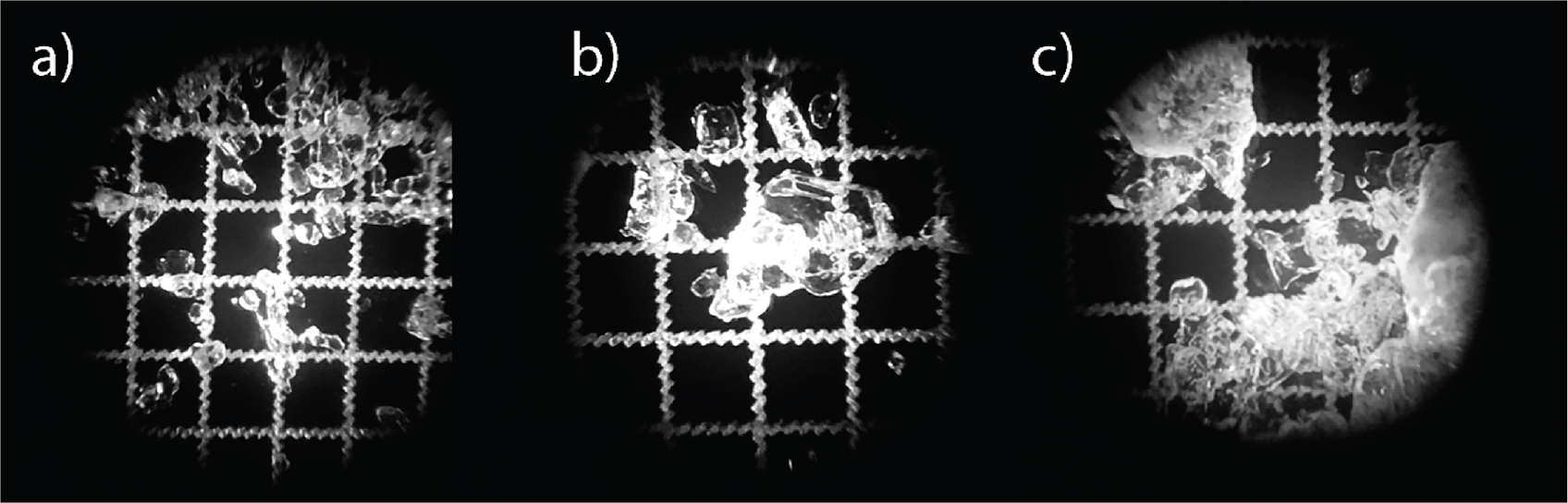
Figure 1. The three types of natural snow used in the experiment: a) 0.2–0.5 mm wind slab rounded grains (WS), b) 0.5–2 mm faceted grains (FC) and c) 0.2–5 mm melt-freeze clusters (MF). The grid scale is 1 mm.

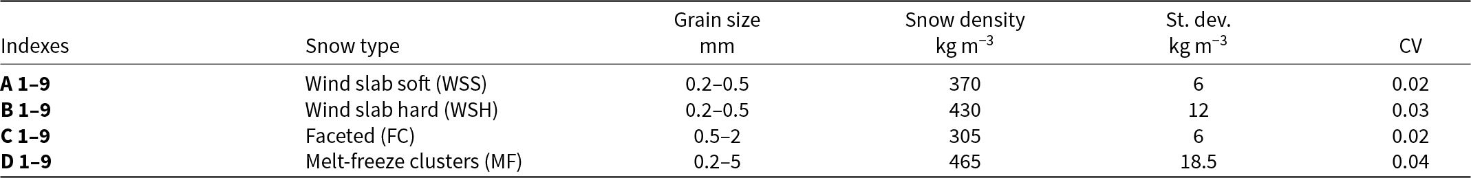
Table 1. Snow type, grain size, and initial average density together with their standard deviation (st. dev) and coefficient of variance (CV)

Melt-freeze clusters (MF) were collected from the 4-cm-thick bottom layer composed of dense and hard melt-freeze firn. Since this layer experienced substantial temperature gradient metamorphism from a previous melting event, the grains had become somewhat faceted. The collected snow was filtered through a 5-mm sieve to remove large icy particles and make the sample more homogeneous. Faceted crystal samples (FC) were collected from the middle layer of the snowpack. This layer also experienced strong temperature gradients, but no melt, and thus consisted of large faceted and depth hoar crystals formed from the original soft wind slab. This snow was sampled and sieved through 1- and 2-mm sieves. Wind slab (WS) snow was composed of small, rounded grains and was sampled from the top, relatively fresh soft wind slab layer. This snow also experienced a strong temperature gradient for only a short time and therefore had limited faceting on the rounded grains. This snow was filtered through 1-mm sieve. In summary, we produced significant volumes of three snow types after sieving from which samples could be acquired (Figure 1 and Table 1).

The sieved snow was then used to fill 20-cm-high plastic transparent tubes with a diameter of 8-cm to produce as homogeneous samples as possible. Altogether, 36 tubes were filled with sampled snow: the first 18 tubes were filled with WS snow, the next nine with FC snow and the last nine with MF clusters. Snow was manually compressed using a round plastic plate with an 8-cm diameter and a flat bottom surface to achieve desired densities typical of snow types found in sea ice environments (Sturm and Massom, 2009). All samples were placed at the field site and left for two days under sub-zero temperatures to produce sintered snow samples. By using transparent plastic tubes and a compaction technique we improved the measurement protocol suggested by (Mallett and others, 2024). Transparent tubes enabled us to observe change in brine migration daily, while compaction techniques reduced the unwanted effect of heterogeneous compaction of snow at the edges of the cutter when cutting snow samples from snow strata manually. After two days, all samples were weighted and numbered. The bulk density, standard deviation and coefficient of variance were calculated (Table 1).

Each sample was placed in a previously prepared snow ‘farm,’ a container built of snow to protect the samples from melting, wind, and rapid changes in air temperature (Figs. 2, 3). Each row of the farm hosted nine tubes filled with sieved snow.

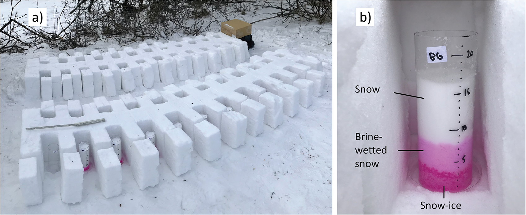
Figure 2. a) the snow ‘farm’ with sample tubes placed in individual cells and b) example of snow sample several days after adding brine, exhibiting brine layer separation.

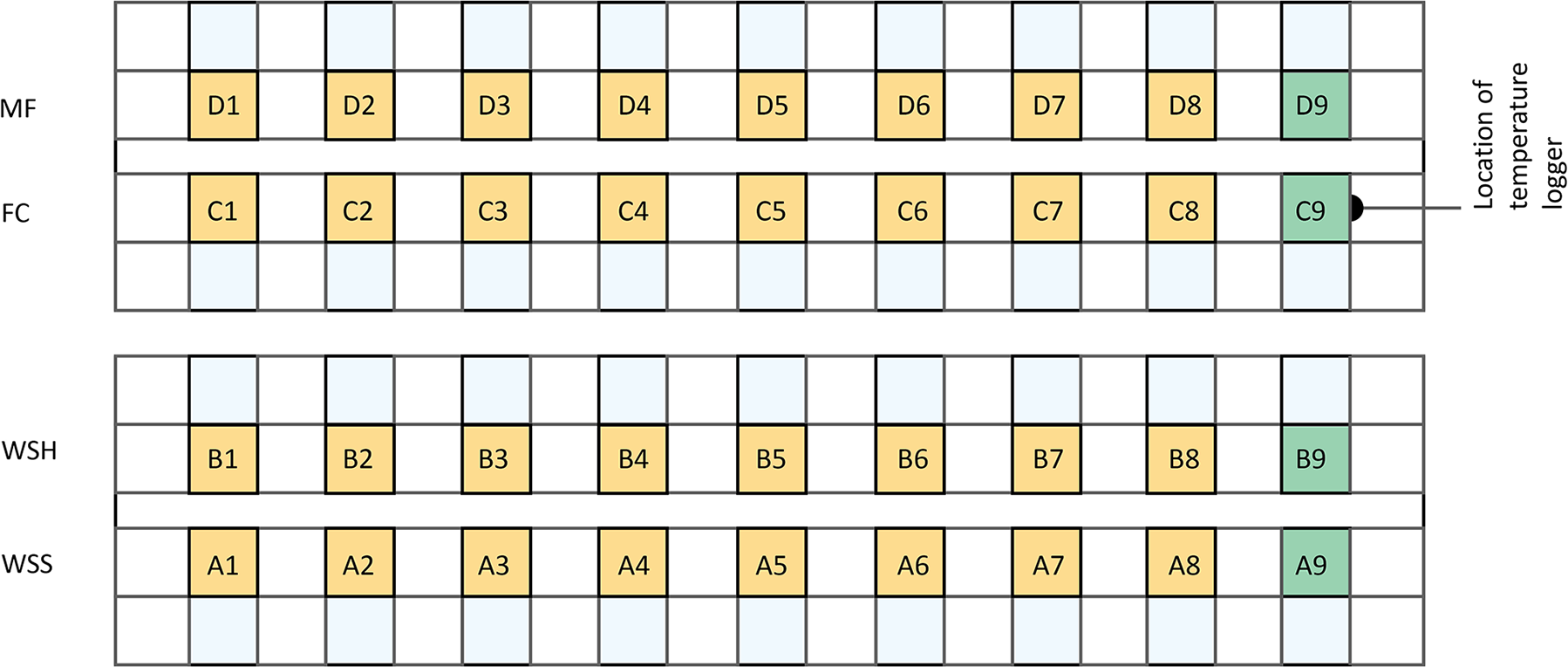
Figure 3. Map of the snow ‘farm’ (top view). Yellow squares represent the samples that wicked 50 ml of brine. Green squares A-C9 represent brine-free (non-saline) reference snow samples. A1-9—soft wind slab B1-9—hard wind slab; C1-9—faceted grains; D1-9—melt/freeze clusters (Table 1).

In the farm, samples were placed into plastic trays filled with a brine solution of known concentration (53.4 ppt) and volume (50 ml). The concentration was higher relative to seawater to ensure that the brine solution did not freeze immediately after adding to the samples. An exception was made for samples A-D 9, which were left brine-free as reference samples. This approach enabled comparison of the compaction rates between the samples with and without brine. To trace brine migration through the snow we added Rhodamine WT dye (Mallett et al., 2024) to the brine. The initial brine and resulting samples salinity was measured with the Orion Star 212A conductivity meter (0.01 ppt resolution; ± 0.5% accuracy) calibrated at three points with the solutions of 1413 µS cm⁻¹, 12.88 mS cm⁻¹ and 99.99 mS cm⁻¹. When brine was added to the samples, the farm bottom surface temperature was −7°C and the brine temperature was −3°C.

To measure the temperature inside the farm we combined manual (Testo 720, accuracy ± 0.5°C) and automatic (Campbell Scientific CR1000/T109, accuracy ± 0.06%) temperature sensors. We also acquired data from the nearby Winnipeg airport weather station to characterize the seasonal progression of Winnipeg weather from hourly time scale air temperature, precipitation and wind speed.

The samples were continuously monitored for 23 days, from February 19 to March 12, 2024. The fieldwork involved measuring snow stratigraphy and sampling to assess snow density, salinity, and snow water equivalent (SWE) across different stratigraphic layers. For the first 5 days, measurements were taken daily, followed by measurements every 2–3 days until the experiment concluded. In total, measurements were acquired on 13 days, with brine wicking levels recorded and salinity and density sampled eight times throughout the experiment.

The measurement protocol involved the following sequential steps:

1. 1. We recorded the temperature in every second cell to assess its variability.

2. 2. Each sample was photographed to determine the height of the snow, the height of brine wicking, and the thickness of the layers.

3. 3. For density and salinity analysis, we took one sample from each row, starting with number 1, and divided it into 2.5 cm segments.

4. 4. The segments were placed in plastic bags, weighed, melted, and measured for salinity, density, and SWE.

The snow height measurement resolution was limited to 1–2 mm, resulting in 5–10% uncertainty in layer density and SWE calculations. Recorded temperature fluctuations (0.6°C standard deviation) within the farm and vertical heterogeneity of the samples could potentially affect the brine wicking processes. However, this was not observed because the variability of wicking height in the samples for the same type and density of snow was negligible in most cases.

3. Weather conditions

Daily averaged air temperature measured at Winnipeg airport was highly variable and ranged from −26.1 to + 5.5°C during the winter (November to March) and from −21.2 to + 2.5°C during the experiment (February 19 to March 12). The mean air temperature during the experiment was −8.1°C. Wind speed exceeded 14 ms⁻¹ at times, leading to wind transport and formation of dense wind slab layers and drifts.

At the bottom of the C9 cell, the average temperature was −5.7°C, which was 2°C warmer than at the top. The minimum temperature was −13.5°C at the bottom and −20°C at the top (Figure 4). The maximum temperature remained just below freezing at the bottom (−0.1°C), while it exceeded freezing at the top (+0.02°C) on the last day of experiment, indicating active snowmelt, leading to compaction at the top of the sample. While a temperature gradient was present inside the samples, it was not strong enough to affect the snow stratigraphy.

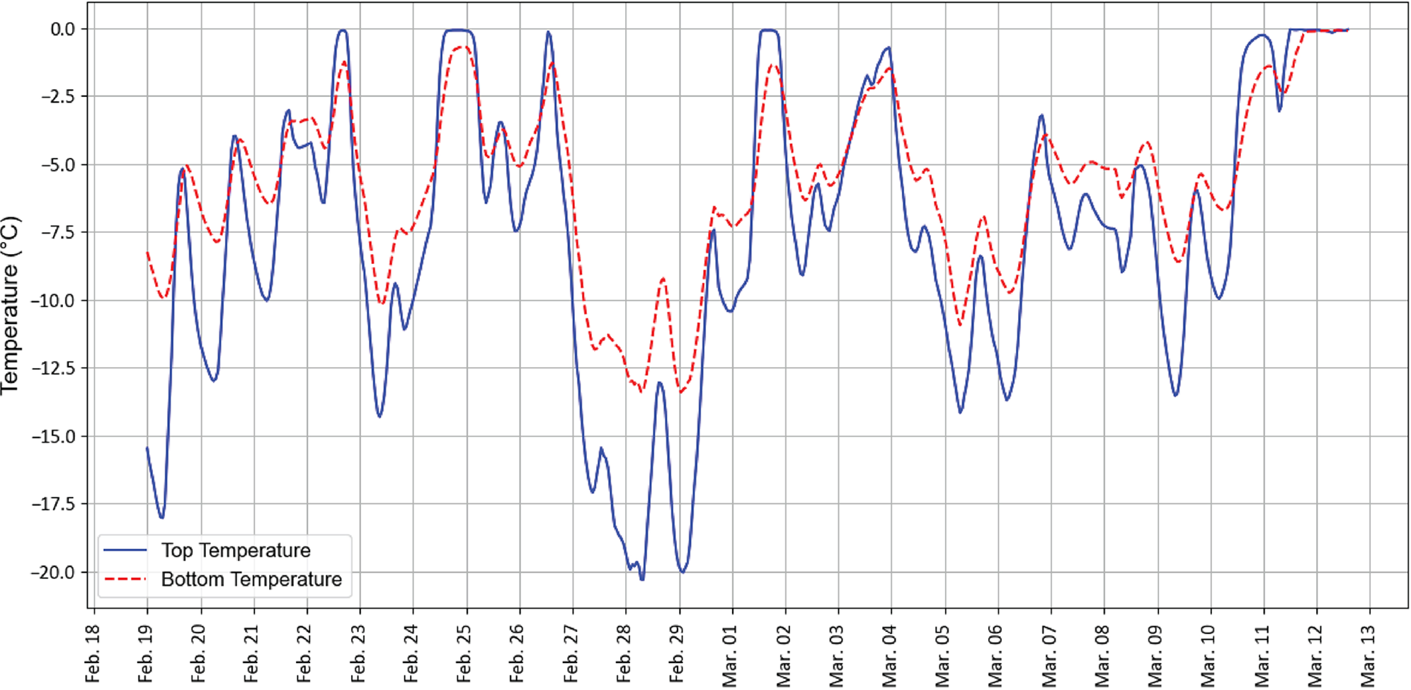
Figure 4. The temperature at the top and the bottom of the C9 snow sample tube measured at 15-min intervals (campbell scientific CR1000/T109 temperature logger). It remained below zero at both levels until the last day of experiment. During thaws temperature in the far reached near-zero values, but did not rise above zero until the last day of experiment.

Because the logger temperature data was obtained at a single cell (C9), we additionally measured temperature in other cells using a manual probe before acquiring other measurements (see protocol). According to this data, the logger point temperature was generally representative of the whole farm, with only slightly higher temperatures compared to the cells located in the center of the farm. The standard deviation of manually measured temperature was on average 0.6°C.

4. Results and data analysis

Our observations of brine migration in snow illustrate that microstructure and density control the height of brine wicking, salinity of brine-affected snow layers, as well as timing and volume of brine runoff from snow samples. The dataset presented in Appendix 1 provides the details of thickness, density, SWE and salinity measurements.

4.1. Brine wicking height

We found that all the added brine volume (50 ml) completely wicked into samples in just a few minutes after their artificial flooding, regardless of snow type or density, and produced a brine-saturated slush at the bottom of the snowpack. The initial brine wicking height varied from 2.1 to 2.7 cm, with slightly higher slush heights in MF and WSH snow compared to FC and WSS samples. Several hours after adding brine, we observed the development of two sublayers with distinctly different properties from the initial brine-saturated slush layer: solid, high-density saline snow-ice at the bottom and less saline brine-wetted snow above it, which retained a snow-like structure during the experiment. These two layers were distinct in color, microstructure, and density, enabling to distinguish them during field measurements. The third uppermost layer was represented by fresh, non-saline (as it was measured during the experiment), unwetted snow.

The thickness of slush/snow-ice layer continued to increase under sub-zero temperatures and reached its near-maximum values by March 2 (day 13) in most samples and demonstrated limited change afterwards until the last day of experiment, when liquid water downward percolation and intensive runoff began. The average thickness of the snow-ice layer was almost the same in the WSS and WSH samples (3.5 cm), indicating no effect of initial sample density on the thickness of this layer. The average thickness of this layer in large-grained MF and FC samples was 23% less (2.7 cm) than in wind slab samples (Figs. 5, 6).

Figure 5. Change in snow layer thickness for a) wind slab soft (WSS), b) wind slab hard (WSH), c) faceted (FC) and d) melt-freeze clusters (MF) snow samples during the 23-day experiment. The dashed lines represent the averages across samples of all types. Black dots represent dates of first brine runoff. Note that the top of the brine-wetted snow moves slowly upward about the same rate as the top of snow-ice layer suggesting coupled movement.

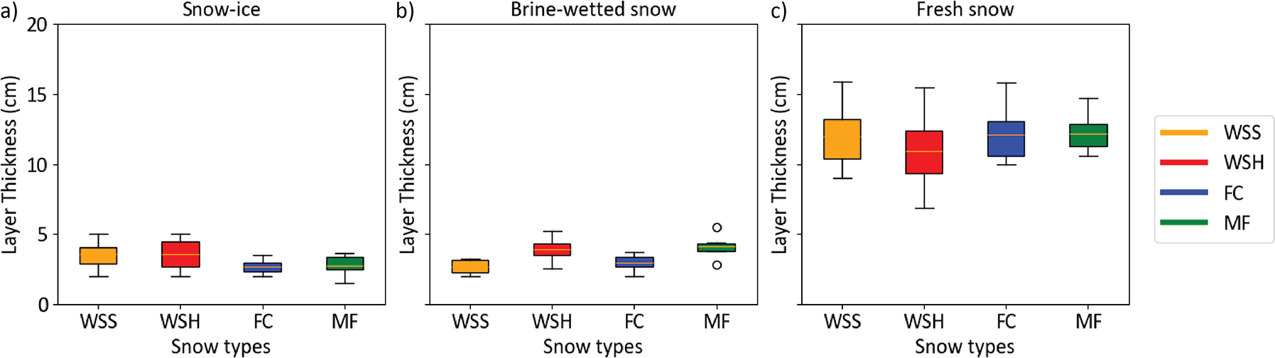
Figure 6. Box-with-whiskers plots of the layer thickness of a) snow-ice, b) brine wetted snow and c) fresh (non-saline) snow above it amongst the four snow types.

The brine-wetted layer developed in all samples within a day after the formation of the bottom slush layer and this process continued until the end of experiment. In all the snow types there was a rapid increase in the thickness of the brine-wetted layer during the first 24 hours. Then, it slowed down and continued at a diminishing rate until the last day of experiment when snowmelt began, and the thickness of this layer decreased in most samples. The total thickness of the brine-wetted layer remained essentially constant (variability less than 0.6 cm) after the third day of the experiment, moving upwards only as the snow-ice layer thickness increased. As this coupled upward migration took place, it continued to reduce the amount of fresh snow above, while thickening the snow-ice layer at the base. This coupled movement was further confirmed by snow salinity measurements. The average thickness of the brine-wetted layer was the largest in MF and WSH samples (4 cm) and the smallest in the WSS samples (2.7 cm); in FC samples, it was 3 cm. Unlike the snow-ice layer, there was a distinct difference in the thickness of the brine-wetted layer between soft WSS and dense WSH samples.

The total thickness of the brine-affected snow (snow-ice and brine-wetted layers) reached its near-maximum values on March 2 (day 13) and increased very slowly afterwards. The largest average brine wicking height occurred in hard WSH samples (7.1 cm), while in softer WSS samples, it was 17% less (5.9 cm). In MF samples, it was 8% less than in the dense WSH (6.5 cm), and in the FC coarse-grained samples, it was the smallest (5.4 cm), 25% smaller compared to the WSH samples. The absolute maximum height of the brine-affected layers was observed on March 11 (day 22) in all samples except the MF samples, where it was observed on February 29. It reached heights of 6.5 cm, 7.2 cm, 7.5 cm and 8.9 cm in FC, WSS, MF and WSH samples, respectively. This corresponds to the 39% (FC, MF), 42% (WSS) and 50% (WSH) of the total samples’ height on the date of measurement.

The total sample height was reduced from nearly 20 cm on February 19 (day 1) to 15.5–17.5 cm by March 12 (day 23). Snow compaction was nearly twice as fast in brine-affected samples compared to the reference fresh-snow samples, which only compressed from 20 cm to 18–19 cm. The highest compaction rates were observed in low-density WSS and FC samples, while the lowest were typical of the dense WSH and MF samples.

4.2. Brine runoff

Brine runoff was observed in all samples; however, its volume and the timing varied significantly between snow types (Figure 7). The earliest brine runoff was observed in MF samples. The first traces of brine drainage in the tray were observed as early as February 26 (day 8), after a strong thaw during the previous day. The volume of brine in the tray then increased gradually and reached 31.5 ml by March 11 (day 22). Unfortunately, we did not measure the brine runoff volume on March 12 as some brine was lost due to accumulation of wind-blown snow in the tray. However, we believe its volume increased further during the thaw. For FC samples, the first brine runoff was observed on March 2 (day 13). Its volume in the tray increased gradually during the rest of the experiment until it reached 39.2 ml on March 11 (day 22). The last measurement on March 12 (day 23) was lost. Brine runoff started earlier in the denser MF than in the FC snow, indicating weaker capillary powers in MF, probably due to melt of the smallest grains and subsequent increase in the diameter of the brine channels.

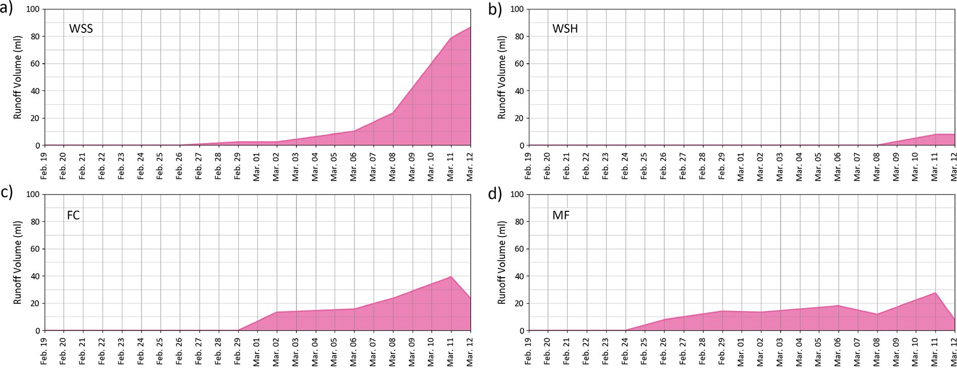
Figure 7. Volume of brine runoff from a) wind slab soft (WSS), b) wind slab hard (WSH), c) faceted (FC) and d) melt freeze clusters (MF) snow samples during the 23-day experiment.

WSS and WSH samples exhibited different runoff patterns compared to FC and MF samples. In WSS sample, the first brine traces were observed on March 6 (day 17); however, the runoff was less rapid then in large-grained samples and its accumulation rate was closer to exponential than linear. The volume of brine in trays increased rapidly during the period March 8–12, because of warm air temperatures on March 11 and 12 and reached 86 ml by the end of experiment. Unlike the other snow types, WSH samples demonstrated the least amount brine runoff. The first brine runoff from WSH snow was observed on March 11 (day 22) only, after the beginning of the March 11–12 warming event. It increased slightly during the next 24 hours and reached a maximum of 8 ml, which was more than ten times less than in WSS samples composed of the same type of snow, but less compacted, indicating the highest capillary retention ability of WSH snow type.

The brine runoff started earlier in the denser MF than in the FC snow, indicating weaker capillary powers in MF, probably due to melt of the smallest grains and subsequent increase in the diameter of the brine channels. In the denser, less porous WSH samples with higher specific surface area compared to WSS, the brine runoff was very limited (8 ml) indicating the highest capillary retention ability, while in WSS samples brine runoff started at least 5 days earlier and was almost 10× greater in magnitude, leading to the total brine runoff volume of 86 ml. This difference in runoff patterns and volume can be crucial for the process of meltwater ponding on sea ice beneath the snow cover.

4.3. Snow density

The density and the compaction rates differed in snow-ice, brine-wetted and fresh snow layers. The snow density increased by 12% in MF samples and by 30% in WSS, WSH, and FC samples after the addition of brine, whereas the reference brine-free snow samples exhibited only a modest increase of 4–11% in density by the end of the experiment. The vertical distribution of snow density in both snow-ice and brine-wetted layers changed over time and became less homogeneous by the end of experiment, with higher density at the bottom and lower density at the top of each layer. This gradient was stronger in WSS and FC samples compared to the denser WSH and MF.

From the 2.5 cm segments, we calculated the average density of snow layers (Appendix 1) and found that the average density of the snow-ice layer was in a range of 771 kg·m⁻³ (WSS) to 877 kg·m⁻³ (WSH). In FC and MF samples, the average densities of the snow-ice layer were 885 kg·m⁻³ and 834 kg·m⁻³, respectively. Thus, the snow-ice layers had similar average densities of nearly 850 kg·m⁻³ regardless of the snow type, with a slightly smaller density in WSS (Figure 8). While the thickness of the layer increased over time, its density did not exhibit a trend during the experiment. It was also found that the bottom of the snow-ice layer was less porous and 20–30% denser compared to the top half of it. Thus, the vertical density distribution within the snow-ice layer was not homogeneous and the density interface within the layers was not as sharp as the difference in the bulk density between these layers.

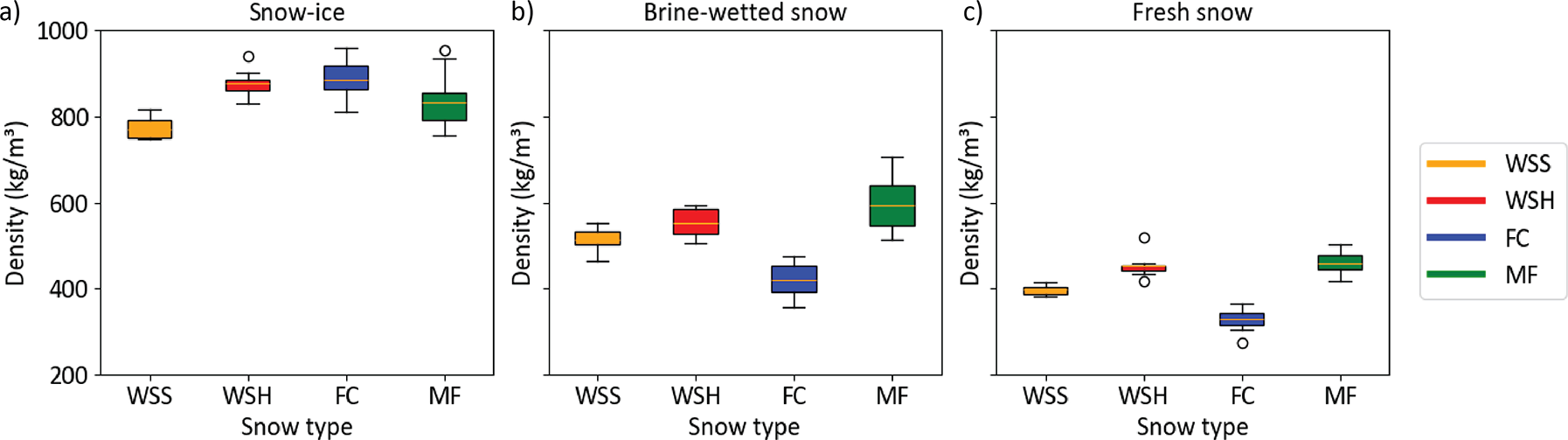
Figure 8. Box-and-whisker plots of the snow density of a) snow-ice layers, b) brine wetted layers and c) fresh (non-saline) snow above it amongst the four snow types.

The average density of the brine-wetted layer was nearly 40–50% that of the snow-ice layer and varied from 420 kg·m⁻³ (FC) to 590 kg·m⁻³ (MF). In the fine-grained WSS and WSH samples, it was 512 and 551 kg·m⁻³, respectively. Thus, it was not consistent between snow types but correlated well with initial snow density. Like the snow-ice layer, the brine-wetted layer density did not change significantly during the experiment but increased during the last two days due to enhanced snow compaction and melt under above-freezing air temperatures. The average density of fresh snow did not change as much as the brine-affected layers and varied from 335 kg·m⁻³ (FC) to 465 kg·m⁻³ (MF).

4.4. Snow water equivalent

SWE was computed from measured thickness (mm) and density (kg·m⁻³) of individual layers using the equation:

\begin{equation*}SWE = \sum\limits_{i = 0}^n {\left( {{H_i}*\frac{{{\rho _i}}}{{{\rho _w}}}} \right)} \end{equation*}

where

H_i—snow layer thickness (mm)

ρ_i—density of snow in the layer (kg·m⁻³)

ρ_w—density of water (1000 kg·m⁻³)

Considering the measured snow density, the fraction of the total SWE from brine-affected snow layers ranged from 49% to 67% of the total SWE by the end of experiment (day 23), which was 12–14% larger than the ratio of the height of the brine-affected snow layers to the total samples height (35–55%) (Figure 9).

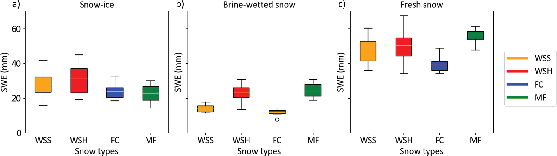
Figure 9. Box-and-whisker plots of snow water equivalent (SWE) of a) snow-ice layers, b) brine wetted layers and c) fresh (non-saline) snow above it in the four snow types.

Moreover, this difference increased over time in samples of all types, with the largest increase in WS samples. While the location of interfaces between snow-ice, brine-wetted and fresh snow layers remained nearly unchanged from day 13 to day 23 of the experiment, the ratio of the SWE changed significantly. This change indicated ongoing snow compaction and melt in the snow-ice and brine-wetted layers and transformation of the bottom portions of brine-wetted snow into snow-ice. This process was followed by upward migration of brine in brine-wetted layer that was compensated by snow compaction, so the location and thickness of the layers remains the same (but not the density and SWE).

4.5. Snow salinity

We calculated the average salinity of the three snow layers from the 2.5 cm segment data (Appendix 1) and found that despite the same initial brine salinity (53.4 ppt), the bulk salinity of the snow-ice layer and brine-wetted layer varied depending on the snow type. The salinity of snow-ice layers was on average two times higher than that of the brine-wetted layers. In the samples that demonstrated the highest brine wicking heights (MF, WSH), the bulk salinity of the snow-ice and brine-wetted layers was lower compared to those in the low-density WSS and FC samples. The average salinity of the snow-ice layer ranged from 15.3 ppt (MF) to 20.3 ppt (FC). In the WSS and WSH samples, the snow-ice layer salinity was on average 19 and 17.6 ppt, respectively (Figures 10, 11). However, the salinity of the snow-ice layers was not constant and gradually decreased during the experiment. In WSS samples, it decreased from 34 to 9 ppt, a larger decrease than in WSH samples where it decreased from 27 to 10 ppt. In FC and MF samples, salinity dropped from 30.5 to 13.7 ppt and from 20.7 to 9.8 ppt, respectively.

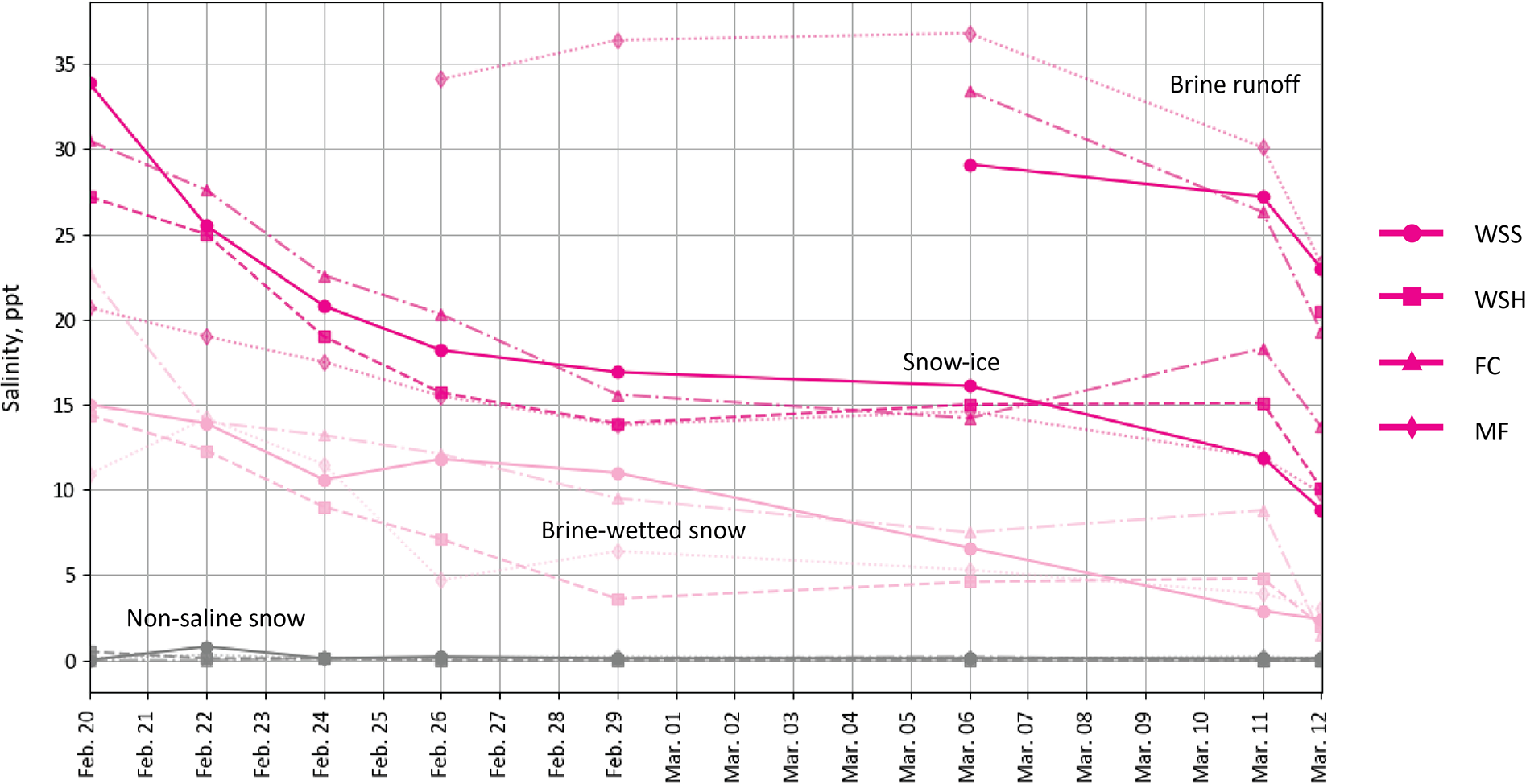
Figure 10. Change in snow sample salinity over time in snow-ice layers, brine wetted layers and fresh (non-saline) snow above it for the four snow types.

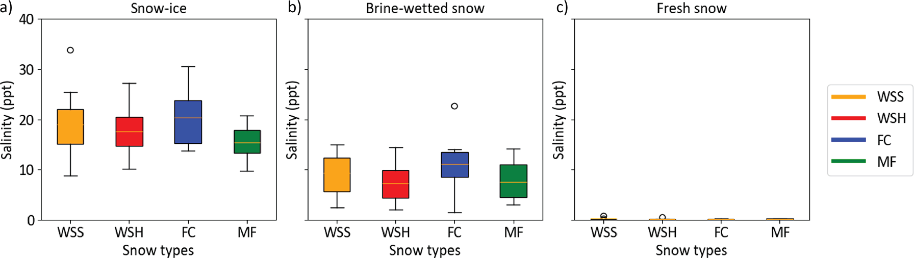
Figure 11. Box-and-whisker plots of the snow salinity in a) snow-ice layers, b) brine wetted layers and c) fresh (non-saline) snow above it amongst the four snow types.

The average salinity ranged from 7.5 ppt (MF) to 11.2 ppt (FC), while in WSS and WSH samples, it was 9.3 and 7.7 ppt, respectively. As for the snow-ice layer, a gradual decrease in snow salinity over time was observed in the brine-wetted layers, decreasing linearly from 15 to 2.4 ppt in WSS and from 14.4 to 2.9 ppt in WSH samples, respectively. However, in FC, it decreased from nearly 23 to 1.5 ppt and from 11 to 3 ppt in MF samples. The salinity of the snow layer above the snow-ice and brine-wetted layers remained negligible in all samples—less than 0.1–0.5 ppt—though trace amounts of brine could be present due to organic inclusions in snow.

By the end of experiment, we observed convergence of the salinity in both snow-ice and brine-wetted layers in all snow types. On March 12 (day 23), the salinity of snow-ice was nearly the same in all samples and ranged from nearly 10 ppt (WSS, WSH, MF) to 13.7 ppt (FC). The salinity of brine-wetted layer exhibited similar convergence trends and reached the values of 1.5 ppt (FC) to 3 ppt (MF). This strong decrease in salinity can be explained by an increase in the layer thickness due to ongoing brine upward migration and snow compaction, leading to continuous incorporation of new portions of less saline snow near the top boundaries of snow-ice and brine-wetted layers, and by the process of brine flushing from snow during brine runoff events.

Brine rejected from the samples was also collected and salinity of these samples was measured. We found that the salinity of brine drained from MF samples was the highest (32.1 ppt). It was less concentrated in WSS samples (27.4 ppt), while WSH samples were most diluted among all snow types (19.5 ppt) and in FC samples the drained brine concentration was 26.3 ppt.

Brine runoff in MF samples it started earlier than in other snow types. In all samples and regardless of snow type, the brine runoff was more diluted over time. At the end of the experiment the brine runoff concentration dropped significantly in all samples to a range of 19 ppt (WSH, FC) to 23 ppt (WSS, MF). Considering the volume of brine runoff and its concentration, we estimated that nearly 75% of the initial amount of salt introduced to the WSS samples was removed by the end of experiment, while in WSH samples, nearly 95% of initial brine was retained in the tubes and only 5% drained off. In FC and MF samples, nearly 22% and 34% of the initial brine drained on day 22, respectively. Unfortunately, we lost brine from FC and MF samples on the last day of experiment due to wind-driven snow accumulation in trays. However, it was observed that more brine drained from samples between days 22 and 23.

5. Discussion

Our experiment revealed that the process of brine migration in snow can be summarized by several key morphological stages as illustrated in Figure 12. From our observations, the brine initially migrates upwards (a, b, c) until it reaches its maximum height (d) after which it stays at that height in a near-equilibrium state for weeks. However, brine-related processes continue to occur in snow strata during this period, which is indicated by the observed brine runoff (e) despite subzero temperatures. At the end of the experiment, when the snow starts to melt, the rest of the brine is flushed from the snow samples, reducing its salinity to a few ppt (f).

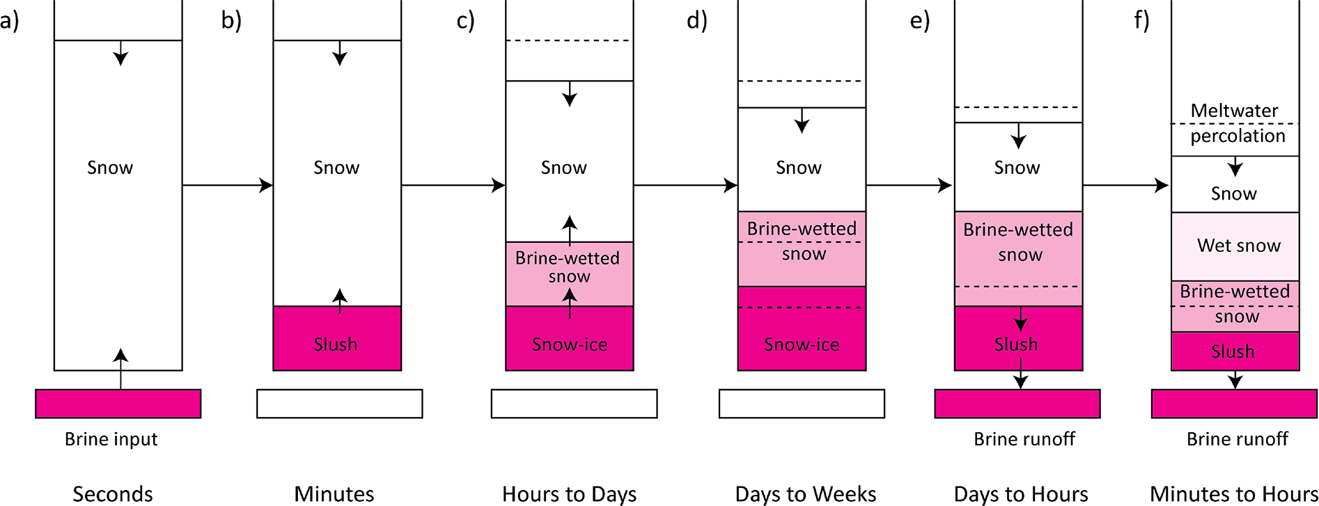
Figure 12. Schematic time series evolution of the formation of snow-ice, brine wicking, snow salinity and density stratification and brine runoff. After initial brine input to the base of the snow, (a) it wicks up rapidly during the first few minutes after introduction (b) and separation of a slush layer begins (c). Snow-ice layer further expands upwards by incorporating the bottom portions of a brine-wetted snow layer which also expands upwards (d). The compaction of snow occurs simultaneously, and it is more intensive in saline layers compared to non-saline snow. When the capillary retention capacity decreases due to changes in snow microstructure and morphology of brine channels, brine runoff begins, resulting in transformation of both saline layers and decrease in their salinity (e). When the snowmelt and meltwater downward percolation reaches the brine-affected layers, a rapid decrease in their salinity occurs due to the flushing of brine from pore space (f). The black arrows indicate the direction of the process and snow layer depth. Dotted lines are the locations of layers interfaces during the previous stage.

Our findings support the results of previous studies on liquid migration through the snow matrix and confirm that brine moves upwards in snow over time and reaches a fixed height. The initial brine rise is driven by capillary action as a function of snow microstructure. However, we are still lacking an understanding on how and why two brine-affected sublayers form, what are the dominant mechanisms of brine migration in these layers, and what is the fraction of liquid water in the layers under different temperature regimes and in different snow types and thicknesses.

5.1. Brine wicking mechanisms

We hypothesize that brine transfer in both slush-snow-ice and brine wetted layers can occur through two mechanisms: capillary rise and molecular/ionic diffusion through the QBL (Figure 13). However, in snow-ice, the volume of brine transferred through pore space due to capillary action is likely much larger compared to molecular diffusion transfer through the QBL. In brine-wetted snow, capillary rise may be possible but is likely limited to a limited number of capillary channels. Nonetheless, these limited capillary channels may be crucial in connecting the network of QBLs and the upward migration of brine. However, more detailed studies with higher temporal and spatial resolution are needed to study this hypothesis and to assess how much salt is transferred separately by each of these processes and how far it could be transferred.

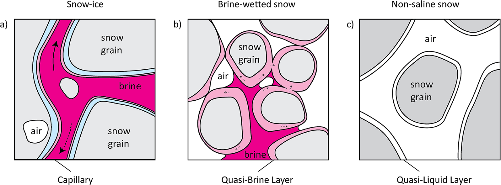
Figure 13. Hypothesized mechanisms of brine transfer in snow-ice (a), brine-wetted (b), and non-saline (c) snow layers. in snow-ice (a), brine is drawn into narrow channels between snow grains due to capillary action, facilitated by the QLL, which enhances the adhesive forces between the brine and the ice surface. when temperatures increase, brine melts the brine channel walls that can lead to brine downward migration and runoff (dotted arrow). With decreasing temperature, brine freezes on the surface of snow grains and the brine channel size decreases, enhancing capillary forces and leading to upward migration (solid arrow). in brine-wetted snow (b), individual brine capillaries may develop, while qbls form a connected quasi-liquid network surrounding the snow grains, with the QBL aiding in the wetting process and spreading of the brine through ionic diffusion. in non-saline snow (c), the QLL exists as a thin, liquid-like layer on the surface of snow grains, influencing inter-grain bonding and other surface interactions in the absence of brine.

5.2. Implications for remote sensing retrievals of snow depth and ice thickness

The introduction of brine-wetted snow is known to alter microwave snow scattering and emission, complicating satellite retrieval processes for snow depth, density and ice thickness (Takizawa, 1985; Drinkwater and Crocker, 1988; Nandan and others, 2017). Increasing amounts of brine-wetted snow result in stronger attenuation of the microwave energy due to an increase in the dielectric loss, which significantly influences the resulting signal retrieved from the passive microwave radiometers and radar altimeters (Barber and others, 1998; Barber and Nghiem, 1999; Tonboe and others, 2021; Stroeve et al., 2022). As a result, microwave emission from brine-wetted snow has a shallower emitting layer (i.e. closer to the air/snow interface); similarly, the dominant scattering horizon for radar altimeters is shifted upwards (Willatt and others, 2010; Nandan et al., 2017; Nandan and others, 2020).

On Antarctic sea ice, fine-grained hard wind slab snow is the most typical snow type and sea water flooding is common (Sturm and Massom, 2009). In the Arctic, the snow on sea ice is composed of softer wind slab and depth hoar snow types are common (Webster and others, 2018), and flooding events are rare. However, the process of brine rejection from growing ice and subsequent wicking into the overlying snow can produce saline snow layers with properties similar to the brine-wetted layer above snow-ice, that we observed.

In our study, after adding brine we observed separation of the initial slush layer into dense snow-ice at the bottom and brine-wetted snow above it. We assume that during the ‘slush’ state of the bottom layer, the microwave signal energy would be absorbed by this layer, altering the waveforms, and limiting the ability to retrieve accurate snow and sea ice thicknesses. During the ‘solid’ snow-ice state of the layer, the microwave signal could demonstrate stronger scattering from the snow-ice/brine-wetted layer interface. However, we did not estimate the volume and fraction of liquid brine in the layers in this study, so more experiments are needed to study this transfer from liquid to solid state and its effect on radar retrievals and mass balance of snow on sea ice.

The interactions between microwave signals and snow in the brine-wetted layer are still not well studied. In our experiment, brine-wetted snow layers retained snow-like structure and contained considerable amounts of brine. We believe most brine in this layer was stored in QBLs on the surface of the snow crystals and assume the increasing thickness of the QBL could influence the microwave signal absorption and backscatter, thus influencing the results of remote sensing retrievals. However, the limits (both height and volume) of brine upward migration through the QBL remain an open question.

6. Conclusion

To study the impact of snow properties on snow brine wicking, we performed a 23-day experiment at the field research site at the University of Manitoba, Winnipeg, Canada. We produced three snow types by compressing natural snow grains (wind slab, faceted grains, and melt-freeze clusters) and observed how the snow type and density affect the brine wicking height, SWE and salinity, position of stratigraphic layers as well as brine runoff timing and volume.

We found that in all the samples, regardless of snow type, the total volume of brine added to samples wicked up into snow and subsequently created two brine-affected sublayers, each with distinctly different physical properties. The slush/snow-ice layer at the bottom was nearly twice as dense and 50% more saline than the brine-wetted layer above, which retained its snow-like structure throughout the experiment. The thickness of the snow-ice layer increased during the experiment due to incorporation of the bottom portions of brine-wetted layer, while brine-wetted layer expanded further upwards, reducing the thickness of fresh, non-saline snow above it. Consequently, along with increasing thickness and SWE of the brine-affected layers, we observed a strong decrease in their salinity that correlated well with changes in layer thicknesses and SWE. The brine wicking mechanisms included capillary forces controlled by snow microstructure and molecular diffusion of brine through QBLs. However, it’s not yet clear how much brine can be transferred by each of these mechanisms at different stratigraphic levels, nor how these transfer mechanisms control the formation of snow-ice and brine-wetted snow sublayers.

The brine wicking height was not constant during the experiment. Brine-affected layers occupied nearly 25% of the total snow height on day 2 and up to 50% on day 23 of experiment. Brine wicking height increased fast during the first 24 hours, then slowed down and stabilized by day 12 in all samples but continued to increase very slowly during the second half of experiment. The highest brine wicking was observed in dense wind slab (WSH). It was on average 25% higher compared to FC samples, 17% higher than in WSS and 8% higher than in MF samples, indicating the influence of snow type and density on brine wicking. However, the average thickness of the snow-ice layer was almost the same in both wind slab samples, and 23% smaller in FC and MF samples. Unlike the snow-ice layer, the average thickness of the brine-wetted layer in WSS snow was 33% smaller than in denser WSH and MF, and 10% smaller than in FC samples.

Brine runoff was observed in all samples by the end of the experiment, demonstrating changes in snow microstructure and its brine retention capacity. WSS and MF samples exhibited the earliest beginning of runoff (days 7–9), while in FC, it started on day 11. It was notable that in denser WSH samples, the runoff process started much later (day 19), and the brine volume was 10× smaller compared to the lower density WSS. Brine runoff was more saline in samples where it occurred earlier compared to those where it occurred on later dates. This difference in brine salinity, volume and runoff patterns can be crucial for the processes of meltwater ponding on sea ice beneath the snow cover and sea ice melt.

The results of the experiment illustrate that snow initial properties affect the height of the brine upward wicking, volume, timing and salinity of brine runoff, as well as density and SWE of brine-affected layers. Because flooding events and considered snow types are common for sea ice environments in Antarctic, the demonstrated differences in brine wicking height and brine salinity could significantly affect estimates of sea-ice mass balance, particularly the microwave remote sensing-based retrievals. Consequently, the information on initial (before flooding) and resulting (after flooding) snow properties and stratigraphy is needed to better estimate brine wicking height and other snow properties.