


1. Introduction
Glide-snow avalanches release directly on the ground in the presence of liquid water between the ground and snowpack (Höller, Reference Höller2014; Ancey and Bain, Reference Ancey and Bain2015). Capillary suction was proposed as a mechanism for the formation of wet snow layers at the soil–snow interface by Mitterer and Schweizer (Reference Mitterer and Schweizer2012). They cited a brown layer of wet snow (about 10 cm) at the base of a glide crack as evidence that this water had originated within the soil. The authors then showed, through simulations, that large hydraulic pressure gradients could lead to water transport from the soil into the snow. This result, along with a review shortly after by Höller (Reference Höller2014); led to increased interest in the role of soil in gliding snow and glide-snow avalanche release (Ceaglio and others, Reference Ceaglio, Mitterer, Maggioni, Ferraris, Segor and Freppaz2017; Fromm and others, Reference Fromm, Baumgärtner, Leitinger, Tasser and Höller2018; Maggioni and others, Reference Maggioni, Godone, Frigo and Freppaz2019). However, aside from the simulations of Mitterer and Schweizer (Reference Mitterer and Schweizer2012); capillary suction across the soil–snow interface has not been investigated in detail. Therefore, it remains unclear if, when, or to what degree capillary suction plays a role in the formation of wet basal layers under gliding snowpacks.
While capillary forces are rarely addressed across the soil–snow interface, they are known to be important in both materials. For example, in both soil and snow, capillary forces are known to be responsible for the formation of capillary barriers (Jordan, Reference Jordan1995; Stormont and Anderson, Reference Stormont and Anderson1999; Avanzi and others, Reference Avanzi, Hirashima, Yamaguchi, Katsushima and De Michele2016) and preferential flow paths (Zhang and others, Reference Zhang, Zhang, Ma, Chen, Akbar, Zhang, Che, Zhang and Cerdà2018; Katsushima and others, Reference Katsushima, Adachi, Yamaguchi, Ozeki and Kumakura2020; Leroux and others, Reference Leroux, Marsh and Pomeroy2020; Nimmo, Reference Nimmo2021). Capillary forces in soil are often characterized with the so-called water retention curve (WRC), which describes the relationship between liquid water content (LWC) and matric potential expressed in units of pressure (tension) or length (head). The WRC is frequently described using models such as those introduced by Brooks and Corey (Reference Brooks and Corey1965) and van Genuchten (Reference van Genuchten1980). These models were subsequently adopted for describing the WRC of snow (Wankiewicz, 1976; Daanen and Nieber, Reference Daanen and Nieber2009).
The WRC of snow has been measured directly in several studies. Initial studies were limited in the number of samples and range of snow properties (Colbeck, Reference Colbeck1974; Reference Colbeck1975; Wankiewicz, 1976; Reference Wankiewicz1978; Jordan, Reference Jordan1983), while more recent studies were more extensive (Yamaguchi and others, Reference Yamaguchi, Katsushima, Sato and Kumakura2010; Reference Yamaguchi, Watanabe, Katsushima, Sato and Kumakura2012; Adachi and others, Reference Adachi, Yamaguchi, Ozeki and Kose2020). Currently, the parameterization by Yamaguchi and others (Reference Yamaguchi, Watanabe, Katsushima, Sato and Kumakura2012) is the most comprehensive. This parameterization is based on drainage experiments of sieved snow and uses the ratio of snow density divided by grain diameter ( $\rho/d$) to determine the shape of the WRC using the van Genuchten model (van Genuchten, Reference van Genuchten1980). Other studies have measured capillary rise (Marsh, Reference Marsh1991; Jordan, Reference Jordan1995; Coléou and Lesaffre, Reference Coléou and Lesaffre1998) and the residual LWC (Colbeck, Reference Colbeck1974; Coléou and Lesaffre, Reference Coléou and Lesaffre1998; Yamaguchi and others, Reference Yamaguchi, Katsushima, Sato and Kumakura2010) but did not describe the full WRC.
In soil science, WRC and van Genuchten parameter data are readily available in large databases (e.g. UNSODA (Nemes and others, Reference Nemes, Schaap, Leij and Wösten2001), EU-HYDI (Weynants and others, Reference Weynants2013)). However, these databases are generally biased toward lower-elevation (agricultural) soils, and there are little data for soils at higher elevations where glide-snow avalanches may occur. Furthermore, discrepancies between WRCs measured in the laboratory and field measurements are well documented (Morgan and others, Reference Morgan, Parsons and Wheaton2001; Iiyama, Reference Iiyama2016; Hedayati and others, Reference Hedayati, Ahmed, Hossain, Hossain and Sapkota2020), with only few field measurements reported in the databases. These discrepancies, along with the lack of alpine soil data, make it difficult to accurately characterize the hydraulic properties of the soil under gliding snowpacks.
Here, we present a quantitative evaluation of capillary suction as mechanism for the formation of wet basal layers at the soil–vegetation–snow interface under gliding snowpacks. For the evaluation, we generated a set of van Genuchten parameters from 40 alpine soil samples in Davos, Switzerland, as well as a field site in the region (Seewer Berg) with glide-snow avalanche activity (Fees and others, Reference Fees, van Herwijnen, Altenbach, Lombardo and Schweizer2025). The van Genuchten model parameters were determined using field measurements of LWC, matric potential and soil texture, as well as snow properties from snow profiles. The resulting WRCs were used to calculate the soil and snow conditions for which capillary flow from the soil into the snow is possible. These conditions were then compared to LWC measurements on Seewer Berg over three winters to determine if capillary suction was possible for the recorded glide-snow avalanches.
2. Methods
2.1. Sites
A total of 40 soil samples were analyzed, with 15 located on the Seewer Berg slope (Davos, Switzerland) and 25 from other locations within the Davos region (Fig. 1). Snow properties were also obtained from manual snow profiles on Seewer Berg. The complete dataset for each soil including coordinates, van Genuchten parameter values and soil texture is available on EnviDat (https://www.doi.org/10.16904/envidat.571).

Figure 1. Map of the soil sample locations near Davos, Switzerland. The inset shows the Seewer Berg (SWB) slope with the location of grid sensors (Gx), profile sensors (Px), snow profiles and the snow liquid water content (LWC) sensors. The Davos region (Rx) soil locations (red) are from various locations near Davos. The coordinates are in Swiss coordinate system (LV95) in meters.
2.1.1. Seewer Berg
The Seewer Berg field site is a predominantly southeast-facing slope with regular glide-snow avalanche activity at 1800 m a.s.l. on Dorfberg above Davos, Switzerland (Fees and others, Reference Fees, van Herwijnen, Altenbach, Lombardo and Schweizer2025). The site has a grid of LWC sensors (Teros 11, Meter Group, Pullman USA/Munich DE) at a depth of 5 cm at 8 m spacing (denoted as SWB G01–SWB G13 and together as SWB Gx, Fig. 1), as well as LWC sensors (Teros 11) in two vertical profiles located ∼1.5 m from each other (denoted as SWB P01 and SWB P02, and together as SWB Px, Fig. 1). These two profiles are adjacent to a profile of matric potential sensors (Tensiomark, ecoTech Umwelt-Messsysteme GmbH, DE). The matric potential sensors are ∼0.5 m from SWB P01 and 2 m from SWB P02. For SWB Px, matric potential and LWC sensors at a depth of 5 cm were used. The standard manufacturer calibrations were used for all soil sensors. In addition to the soil sensors, an LWC sensor (EC-5, Meter Group, Pullman USA/Munich DE) was installed on a metal wedge near the vertical soil profiles at a height of 5 cm above the ground. This sensor was calibrated for snow in the lab (Fees and others, Reference Fees, Lombardo, van Herwijnen, Lehmann and Schweizer2024a). Additional descriptions of the site and the glide-snow avalanche activity are provided by Fees and others (Reference Fees, van Herwijnen, Lombardo, Schweizer and Lehmann2024b; Reference Fees, van Herwijnen, Altenbach, Lombardo and Schweizer2025) and Fees and others (Reference Fees, Lombardo, van Herwijnen, Lehmann and Schweizer2024a).
A soil profile was sampled at the location of SWB P01 prior to sensor installation. The soil density was determined by sampling a known volume of soil that was dried at  $105^{\circ}\mathrm{C}$ and weighed. The fine earth was separated through a 2 mm sieve, and the remaining skeleton was weighed. The volume of the skeleton was calculated assuming a density of $2650\ \mathrm{kg\ m}^{-3}$. The bulk density (BD) of the soil was calculated using the volume and mass of the entire soil sample, including the skeleton (volumetric skeleton fraction of 4.3%). Grain size measurements followed the definition of sand ranging from 2 mm to 63 μm, silt from 63 μm to 2 μm and clay less than 2 μm. Samples were treated with a 30% hydrogen peroxide solution to remove organic matter before using the pipette method by Gee and Bauder (Reference Gee and Bauder1986) to determine grain size distribution.
In addition to the soil data from Seewer Berg, snow properties (density (ρ) and grain diameter (d)) were acquired from manual snow profiles taken regularly at a reference site (Fig. 1) as well as from the avalanche crown after avalanches released on the Seewer Berg slope. For each avalanche, profiles from the reference site were available 3–5 days prior to release and 3–5 days after release at the reference site and crown. An exception is the 25 March 2024 avalanche, for which a profile prior to release was only available 17 days before the event. The values for the lowest recorded snow layer were used (typically the first 5 cm to 10 cm above the ground). The grain types included small rounded grains, melt forms and occasionally rounding faceted particles as a secondary grain type (Fierz and others, Reference Fierz, Armstrong, Durand, Etchevers, Greene, McClung, Nishimura, Satyawali and Sokratov2009). The grain diameter was taken from the profiles, which were determined with a magnifying glass and crystal card (grid) (Fierz and others, Reference Fierz, Armstrong, Durand, Etchevers, Greene, McClung, Nishimura, Satyawali and Sokratov2009). The density was measured with a  $100\ \mathrm{cm}^{3}$ cylindrical density cutter and balance.
2.1.2. Region Davos
A total of 25 locations were sampled for density and soil texture along elevation gradients (2000–3000 m a.s.l.) on amphibolitic, gneissic and calcareous bedrock near Davos, Switzerland (DAV R01–DAV R25, together DAV Rx). A volume proportional excavation approach was chosen for BD analysis because of the rocky conditions in alpine soils (Holmes and others, Reference Holmes, Wherrett, Keating and Murphy2012). Samples were excavated at 0–5 cm or 5–10 cm, sieved and weighed in the field, and an aliquot was taken for lab analysis. The sample volume was measured with a measuring stick. Due to the high skeleton fractions (average volumetric fraction of 23%), the BD of the fine earth was used, which was calculated as
 \begin{equation}
\mathrm{BD} = \dfrac{M_{\mathrm{s}} - M_{\mathrm { \gt 2mm}}}{V_{\mathrm{s}} - \dfrac{M_{\mathrm{ \gt 2mm}}}{\rho_{\mathrm{ \gt 2mm}}}}
\end{equation}
\begin{equation}
\mathrm{BD} = \dfrac{M_{\mathrm{s}} - M_{\mathrm { \gt 2mm}}}{V_{\mathrm{s}} - \dfrac{M_{\mathrm{ \gt 2mm}}}{\rho_{\mathrm{ \gt 2mm}}}}
\end{equation} where  $M_{\mathrm{s}}$ is the dry mass of the whole sample in kg, $M_{\mathrm{ \gt 2mm}}$ is the mass of the stone fraction in kg, $V_{\mathrm{s}}$ is the volume of the sample measured in the field in $\mathrm{m}^{3}$ and $\rho_{\mathrm{ \gt 2mm}}$ is the stone density of $2650\ \mathrm{kg\ m}^{-3}$.
Grain size of the fine earth was determined following the same method as for the SWB P01 soil profile described above. For locations where texture and BD were only measured at 5–10 cm depth, these values were assumed to be the same for the surface layers (0–5 cm).
2.2. Water retention properties
The water retention properties of the soil and snow were parameterized with the van Genuchten model (van Genuchten, Reference van Genuchten1980) as
 \begin{equation}
\theta\left(h\right) = \theta_{\mathrm{r}} + \frac{\left(\theta_{\mathrm{s}} - \theta_{\mathrm{r}}\right)}{\left[ 1 + \left( \alpha h \right)^n \right]^m}
\end{equation}
\begin{equation}
\theta\left(h\right) = \theta_{\mathrm{r}} + \frac{\left(\theta_{\mathrm{s}} - \theta_{\mathrm{r}}\right)}{\left[ 1 + \left( \alpha h \right)^n \right]^m}
\end{equation} which describes the relationship between the matric potential (h, expressed here as the absolute value of the negative matric potential head) and LWC (θ) with five parameters: residual LWC ( $\theta_{\mathrm{r}}$), saturated LWC ( $\theta_{\mathrm{s}}$), α, n and m (Eqn (2)). Here, m was set equal to $1-1/n$ (van Genuchten, Reference van Genuchten1980). Throughout the paper, h is cm of water, α is in $\mathrm{cm}^{-1}$, LWC values are volumetric and expressed in fractions and n is unitless. Saturation is expressed as the effective saturation (S) (van Genuchten, Reference van Genuchten1980)
 \begin{equation}
S = \frac{\theta - \theta_{\mathrm{r}}}{\theta_{\mathrm{s}} - \theta_{\mathrm{r}}}
\end{equation}
\begin{equation}
S = \frac{\theta - \theta_{\mathrm{r}}}{\theta_{\mathrm{s}} - \theta_{\mathrm{r}}}
\end{equation} which differs from the saturation defined by the water filled fraction of the porosity. While  $\theta_{\mathrm{r}}$ and $\theta_{\mathrm{s}}$ have direct physical meanings as the minimum and maximum amount of water, α and n are more loosely related to the inverse of the air-entry pressure and width of pore-size distribution, respectively (van Lier and Pinheiro, Reference van Lier and Pinheiro2018).
2.2.1. Seewer Berg
Four methods were used to obtain the van Genuchten parameter values for the 15 soil samples on Seewer Berg (SWB Gx and Px): (i) the inverse solution method in numerical simulations of unsaturated flow using Hydrus-1D (Simunek and others, Reference Simunek, van Genuchten and Sejna2008), (ii) direct fitting of LWC and matric potential measurements and the pedotransfer functions (PTFs) by (iii) Wessolek and others (Reference Wessolek, Kaupenjohann and Renger2009) and (iv) Szabó and others (Reference Szabó, Weynants and Weber2021).
Hydrus-1D was used to determine the van Genuchten parameter values for the Seewer Berg soils (SWB Gx and Px). Hydrus numerically solves the Richards equation (Richards, Reference Richards1931) and was initialized with 301 nodes over 20 cm soil depth with the measured LWC at 5 cm. The lower boundary condition was set to free-drainage while the upper boundary condition utilized daily precipitation and evaporation data from the nearby Davos DAV MeteoSwiss station (1594 m a.s.l). θs was fixed to the maximum daily value during the simulated time period while all other variables were fit with the model. A time series of daily averaged LWC values (15 min resolution, 5 cm depth) from 1 May 2023 to 30 September 2023 were fit. Not all sensors could be successfully fit and these 9 sensors (22 total) were therefore excluded (see Discussion).
Direct fitting was used to determine the van Genuchten parameter values for the SWB Px soils. For the direct fitting, the WRC was fit directly to daily matric potential and LWC values at 5 cm for 15 April 2023 to 5 November 2023 using Eqn (2). The data were geometrically binned with respect to the matric potential and the largest LWC value of each bin was taken to approximate the main drying curve (see Fig. A1 and A2 in the Appendix). This was necessary due to the highly hysteretic nature of the measurements (see Discussion). The same matric potential measurements were used for both LWC measurements the Seewer Berg soil profiles (SWB P01 and SWB P02).
PTFs are functions that relate readily available or easily measurable soil properties (e.g. soil texture, density, pH) to more complicated or less readily available soil properties (e.g. hydraulic parameters). The PTFs by Wessolek and others (Reference Wessolek, Kaupenjohann and Renger2009) and Szabó and others (Reference Szabó, Weynants and Weber2021), hereafter referred to as the Wessolek and EuroV2 PTFs, respectively, were used to determine the van Genuchten parameter values for SWB P01 (density and texture were not measured at SWB P02). The PTFs determine the van Genuchten parameter values from a set of underlying physical soil measurements such as soil texture and BD. The Wessolek PTF was trained on forest, meadow and pasture soils in Germany (Wessolek and others, Reference Wessolek, Kaupenjohann and Renger2009), while the EuroV2 PTF is based on a broad range of soils from Europe (Weynants and others, Reference Weynants2013). The soil texture and BD of SWB P01 were used with the EuroV2 PTF using the ‘VG’ output. For the Wessolek PTF, only soil texture was used. The resulting textural class, Ls4 (German soil classification system KA5 (Eckelmann, Reference Eckelmann2009)), was chosen as the reference soil for future calculations because it resulted in the maximum capillary suction for any of the Seewer Berg soils (SWB Gx or Px) with any method. According to the USDA classification (Soil Survey Staff, 1999), SWB 01 corresponds to a sandy loam (Fig. 2).
2.2.2. Region Davos
The van Genuchten parameter values of the Davos region soils (DAV Rx) were determined using the Wessolek and EuroV2 PTFs. As with SWB P01, the soil texture was used with the Wessolek PTF, while the soil texture and BD were used with the EuroV2 PTF. No BD was measured for DAV R17 and DAV R25 and was therefore not included in the EuroV2 calculation for these soils. The Wessolek PTF resulted in ten soil textural classes (German soil classification system): Ts4, St3, Ls4, Sl3, Sl2, Su2, Ss, Lts, Sl4, Su3. According to the USDA classification (Soil Survey Staff, 1999), the DAV Rx soils were classified as sandy clay loam, sandy loam, loamy sand and sand (Fig. 2).

Figure 2. Soil texture distribution of the DAV Rx soils and SWB P01 according to the USDA classification (Soil Survey Staff, 1999). C: clay, SiC: silty clay, SiCL: silty clay loam, CL: clay loam, SC: sandy clay, SCL: sandy clay loam, Si: silt, SiL: silty loam, L: loam, SL: sandy loam, LS: loamy sand, S: sand.
2.2.3. Snow
For snow, α and n were calculated as a function of  $\rho/d$ using the parameterization by Yamaguchi and others (Reference Yamaguchi, Watanabe, Katsushima, Sato and Kumakura2012). To account for hysteresis between the drying and wetting curves (Adachi and others, Reference Adachi, Yamaguchi, Ozeki and Kose2020; Leroux and others, Reference Leroux, Marsh and Pomeroy2020), the relationship $\alpha_{\mathrm{wetting}} = 1.4\alpha_{\mathrm{drying}}$ was used (Adachi and others, Reference Adachi, Yamaguchi, Ozeki and Kose2020). No hysteresis in n was considered (Adachi and others, Reference Adachi, Yamaguchi, Ozeki and Kose2020). $\theta_{\mathrm{r}}$ and $\theta_{\mathrm{s}}$ were set to 0.02 (Yamaguchi and others, Reference Yamaguchi, Watanabe, Katsushima, Sato and Kumakura2012) and the porosity, respectively.
Based on the snow profiles,  $\rho/d$ values of $0.2\times10^{6}\ \mathrm{kg\ m}^{-4}$, $0.4\times10^{6}\ \mathrm{kg\ m}^{-4}$ and $1.2\times10^{6}\ \mathrm{kg\ m}^{-4}$ were determined to be representative of the minimum, average and maximum $\rho/d$ ratios, respectively. We define the average $\rho/d$ ratio ( $0.4\times10^{6}\ \mathrm{kg\ m}^{-4}$) as the ‘reference snow’ for the remainder of the paper. It should be noted that there are many combinations of densities and grain sizes that result in the same $\rho/d$ ratio. For example, the reference snow ratio of $0.4\times10^{6}\ \mathrm{kg\ m}^{-4}$ can be obtained with a density of $400\ \mathrm{kg\ m}^{-3}$ and a grain diameter of 1 mm, or snow with a density of $300\ \mathrm{kg\ m}^{-3}$ and a grain diameter of 0.75 mm.
2.3. Suction envelope
To assess the conditions under which capillary suction from the soil into the snow could occur, we introduce what we are calling the suction envelope (Fig. 3). The suction envelope shows the LWC of the basal snow for combinations of soil saturation and depth, when the system is in hydrostatic equilibrium (balance between gravity and capillary forces). Each point is extracted from an equilibrium LWC profile (Fig. 4) with the matric potential head (absolute value) equal to the distance from a free water table (i.e. constant pressure lower boundary condition). Points within the envelope result in an equilibrium LWC of the basal snow of at least 0.5% above  $\theta_{\mathrm{r}}$ (colored region in Fig. 3), while conditions resulting in LWC of less than 0.5% above $\theta_{\mathrm{r}}$ are considered to be outside of the envelope (white region in Fig. 3). Thus, points within the suction envelope would lead to capillary rise into dry snow ( $\mathrm{LWC}_{\mathrm{snow}}=\theta_{\mathrm{r}}$), resulting in the LWC shown in Fig. 3 (when $\mathrm{LWC}_{\mathrm{snow}}\geq\theta_{\mathrm{r}}\,+\,0.5\%$).
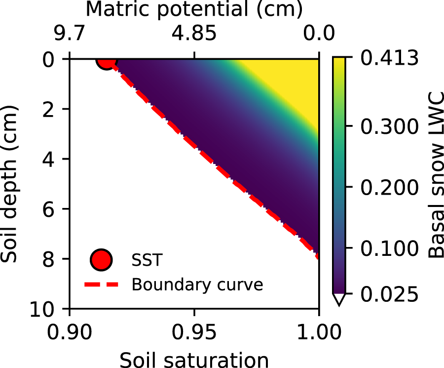
Figure 3. A suction envelope for the reference soil and snow. The colored region indicates the LWC of the lowermost snowpack layer at the vegetation–snow interface. The white area represents soil saturation and depth combinations that do not result in capillary suction (defined as 0.5% above the residual water content, here  $\theta_{\mathrm{r}}=2$%). The boundary curve indicates the minimum soil saturation that allows for capillary suction at a given soil depths. The SST is the value of the boundary curve at a soil depth of 0 cm. The absolute value of the negative soil matric potential is provided on the upper x-axis as a reference to the corresponding soil saturation.
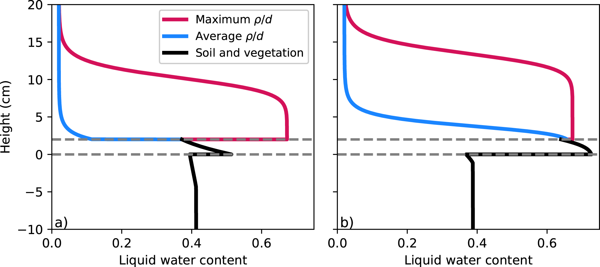
Figure 4. Vertical LWC profiles for average (reference snow,  $\rho/d=0.4\times10^{6}\ \mathrm{kg\ m}^{-4}$) and maximum $\rho/d$ ( $1.2\times 10^{6}\ \mathrm{kg\ m}^{-4}$) ratios (snow density/grain diameter) with (a) German soil texture class Ls4 (reference soil) and (b) German soil texture class Ss (resulted in the lowest surface saturation thresholds (SSTs)). The dashed gray lines indicate the location of the 2 cm thick vegetation layer with soil below and snow above. Both profiles use a soil saturation of 0.95 at 0 cm.
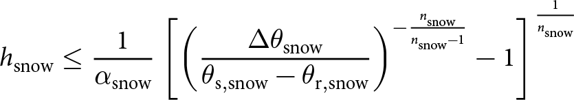
Mathematically, points within the suction envelope satisfy the condition (derived from Eqns. (2) and (3))
 \begin{equation}
h_{\mathrm{snow}} \leq \frac{1}{\alpha_{\mathrm{snow}}}
\left[
\left(
\frac{\Delta\theta_{\mathrm{snow}}}{\theta_{\mathrm{s,snow}}-\theta_{\mathrm{r,snow}}}\right)^{-{\frac{n_{_{\mathrm{snow}}}}{n_{_{\mathrm{snow}}}-1}}}-1\right]^{\frac{1}{n_{_{\mathrm{snow}}}}}
\end{equation}
\begin{equation}
h_{\mathrm{snow}} \leq \frac{1}{\alpha_{\mathrm{snow}}}
\left[
\left(
\frac{\Delta\theta_{\mathrm{snow}}}{\theta_{\mathrm{s,snow}}-\theta_{\mathrm{r,snow}}}\right)^{-{\frac{n_{_{\mathrm{snow}}}}{n_{_{\mathrm{snow}}}-1}}}-1\right]^{\frac{1}{n_{_{\mathrm{snow}}}}}
\end{equation} where  $\Delta\theta_{\mathrm{snow}}$ is the capillary suction threshold (here, 0.5%) and is equal to
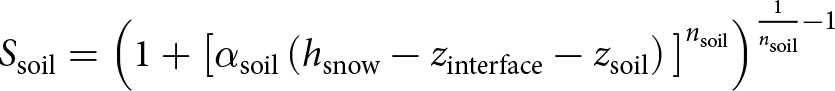
  $\theta_{\mathrm{snow}}-\theta_{\mathrm{r,snow}}$. The suction envelope considers soil and snow separated by 2 cm of vegetation (Fig. 4), since many glide-snow avalanches occur on vegetated slopes (Höller, Reference Höller2014; Maggioni and others, Reference Maggioni, Godone, Frigo and Freppaz2019), including Seewer Berg (Feistl and others, Reference Feistl, Bebi, Dreier, Hanewinkel and Bartelt2014). Thus, the relationship between $h_\mathrm{snow}$ and the soil saturation ( $S_{\mathrm{soil}}$) at a soil depth ( $z_{\mathrm{soil}}$) is
 \begin{equation}
S_{\mathrm{soil}} = \Big(1+
\big[\alpha_{\mathrm{soil}}
\left(h_{\mathrm{snow}}-z_{\mathrm{interface}}-z_{\mathrm{soil}}\right)
\big]^{n_{\mathrm{soil}}}
\Big)^{\frac{1}{n_{\mathrm{soil}}}-1}
\end{equation}
\begin{equation}
S_{\mathrm{soil}} = \Big(1+
\big[\alpha_{\mathrm{soil}}
\left(h_{\mathrm{snow}}-z_{\mathrm{interface}}-z_{\mathrm{soil}}\right)
\big]^{n_{\mathrm{soil}}}
\Big)^{\frac{1}{n_{\mathrm{soil}}}-1}
\end{equation} where  $z_{\mathrm{interface}}$ is the thickness of the vegetation layer (here, 2 cm).
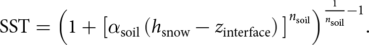
For clarity in subsequent plots and discussion, we define the ‘boundary curve’ as the points along the edge of the suction envelope where  $\Delta\theta_{\mathrm{snow}}=0.5$% (Fig. 3). We also define the ‘surface saturation threshold’ (SST) as the soil saturation of the boundary curve at the soil surface ( $z_{\mathrm{soil}}=0$). In other words, the soil saturation for $z_{\mathrm{soil}}=0$ and $\Delta\theta_{\mathrm{snow}}=0.5$% is given by
 \begin{equation}
\mathrm{SST} = \Big(1+
\big[\alpha_{\mathrm{soil}}
\left(h_{\mathrm{snow}}-z_{\mathrm{interface}}\right)
\big]^{n_{\mathrm{soil}}}
\Big)^{\frac{1}{n_{\mathrm{soil}}}-1}.
\end{equation}
\begin{equation}
\mathrm{SST} = \Big(1+
\big[\alpha_{\mathrm{soil}}
\left(h_{\mathrm{snow}}-z_{\mathrm{interface}}\right)
\big]^{n_{\mathrm{soil}}}
\Big)^{\frac{1}{n_{\mathrm{soil}}}-1}.
\end{equation}The step-by-step calculation is provided in the Appendix.
Since the calculation assumes that the soil and snow are hydraulically connected and are in hydrostatic equilibrium, the WRC of vegetation layer does not need to be considered and the vegetation only serves to add 2 cm of pressure head to the matric potential in the basal snow. The calculation also assumes that all three layers are static and isothermal ( ${0}^{\circ} \mathrm{C}$). No considerations of the rate of water transport, heat transfer or changes to snow microstructure are included.
The points within the suction envelope indicate the LWC of the basal snow, but each point also has a corresponding LWC profile (Fig. 4). For the full vertical profile, the van Genuchten parameter values for the vegetation are needed and were determined by measuring the WRC of Seewer Berg grass sample in the laboratory (see Appendix).
3. Results
3.1. Suction envelope
The suction envelope for the reference snow and soil shows that the LWC of the basal snow increases with increasing soil saturation and decreasing soil depth (Fig. 3). In other words, for the same soil saturation value (S), the basal snow LWC is higher when S is found closer to the surface. For this envelope, the SST is 91.5% and no capillary suction occurs for any soil saturation below a depth of 7.99 cm. The WRC of both the soil and the snow affect the LWC within the snow (Fig. 4).
3.2. Snow properties
The SST increases with increasing  $\rho/d$ (Fig. 5). Capillary suction therefore increases with increasing snow density and decreasing grain diameter. For the realistic values of $\rho/d$ used here, SSTs ranged between 0.84 and 0.94 for the reference soil. The maximum soil depth of the boundary curve also increases with increasing $\rho/d$ from 5.3 to 18.9 cm.
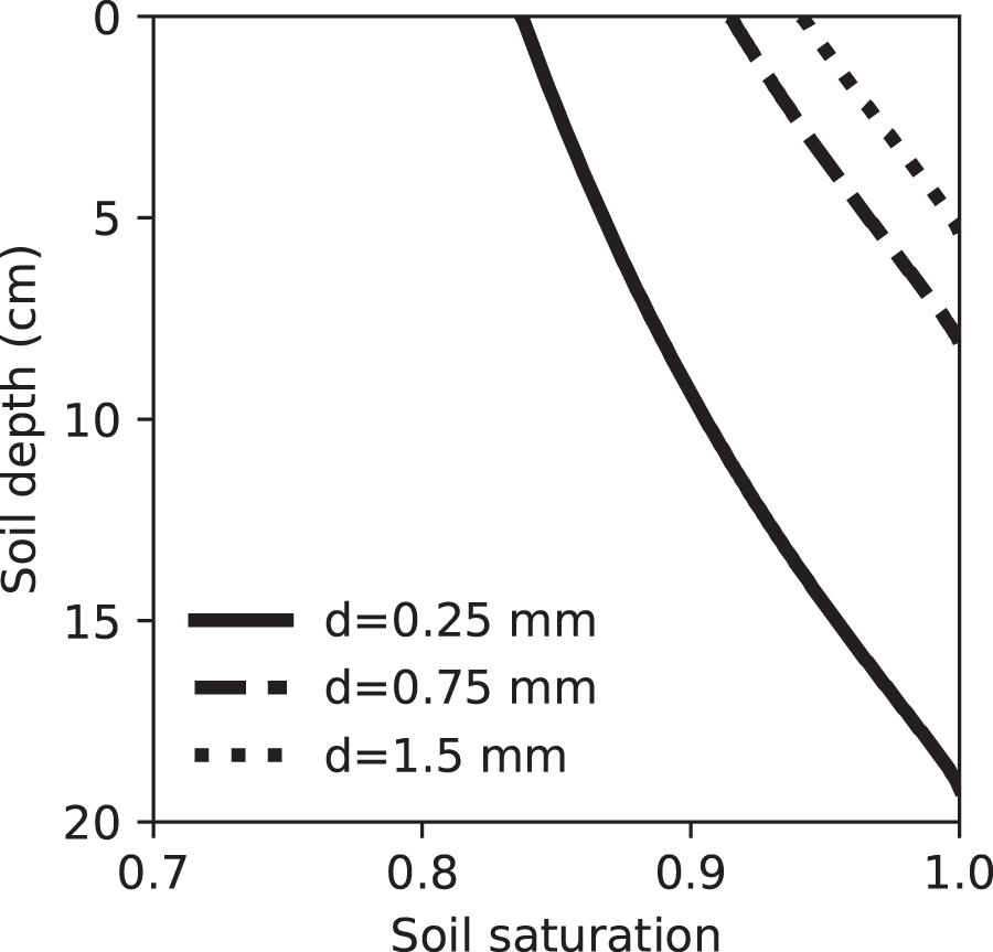
Figure 5. Three boundary curves for the reference soil and snow with a density (ρ) of  $300\ \mathrm{kg\ m}^{-3}$ and three grain diameters (d) corresponding to the minimum ( $\rho/d=0.2\times10^{6}\ \mathrm{kg\ m}^{-4}$, d = 1.5 mm), average ( $\rho/d=0.4\times10^{6}\ \mathrm{kg\ m}^{-4}$, d = 0.75 mm) and maximum ( $\rho/d=1.2\times10^{6}\ \mathrm{kg\ m}^{-4}$, d = 0.25 mm) $\rho/d$ ratios measured on Seewer Berg. The d = 0.75 mm curve corresponds to the suction envelope in Fig. 3.
3.3. Soils
For all soils (with the reference snow), SSTs ranged from 0.70 to 1.00, with a maximum soil depth of 7.99 cm at 100% saturation (Fig. 6). When using the maximum  $\rho/d$, the boundary curves shifted to lower SSTs (0.55–1.0) and greater soil depths (18.9 cm at 100% saturation). This shift is due to the higher capillary forces by the maximum $\rho/d$ snow. The Wessolek PTF resulted in the lowest SSTs while the Hydrus fitting method provided the highest SSTs. The boundary curves are clustered by method and soil.

Figure 6. Boundary curves for each soil and method with two ratios of snow density (ρ) to grain diameter (d). Left: reference (average ratio) snow ( $\rho/d=0.4\times10^{6}\ \mathrm{kg\ m}^{-4}$) and right: maximum ratio ( $\rho/d=1.2\times10^{6}\ \mathrm{kg\ m}^{-4}$). For each side of the plot (average and maximum $\rho/d$), the data are the same in each subplot, with the colors used to indicate soil samples and methods.
For the Davos region soils (DAV Rx), all of the ten texture classes from the Wessolek PTF resulted in lower SSTs than the EuroV2 PTF, except for the Lts soil texture class. The variability of the boundary curves for the Wessolek PTF is larger than the variability for the EuroV2 PTF.
For SWB P01, the Wessolek PTF also resulted in a lower SST than the EuroV2. The highest SST for SWB P01 was obtained with the Hydrus fitting method, while the direct fitting and EuroV2 resulted in similar boundary curves between the two extremes (Fig. 7). The EuroV2 PTF therefore matched the Hydrus and direct fitting methods for SWB P01 better than the Wessolek PTF. Both the Hydrus and direct fitting methods resulted in higher SSTs for SWB P02 compared to SWB P01. The Hydrus fitting method resulted in similar boundary curves for all Seewer Berg soils (SWB Gx and Px).
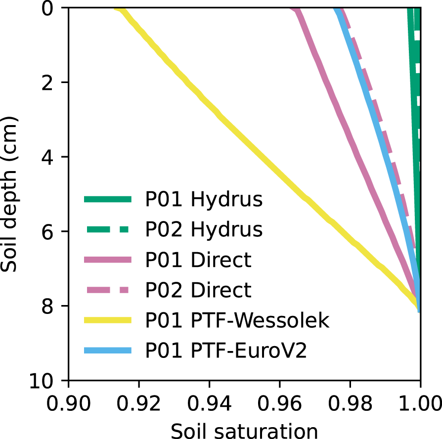
Figure 7. Boundary curves for SWB P01 and SWB P02 with each method using the reference snow.
To conclude, the PTF of Wessolek predicts the smallest soil capillary forces and inverse modeling with Hydrus the strongest capillary effects. This is manifested in the van Genuchten parameter values as discussed next.
3.4. van Genuchten parameter values
Similar to the clustering of the boundary curves in Fig. 6, the van Genuchten parameter values were also clustered by method (Figs. 8 and 9). As shown by the linear fits in Fig. 8, the SST correlated strongly with α, while correlating only weakly with the other parameters. This was verified with the Pearson correlation coefficients ( $r_{\mathrm{p}}$), which were −0.94 (p < 0.001) for α, 0.07 (p = 0.6) for n, 0.25 (p = 0.06) for $\theta_{\mathrm{r}}$ and 0.24 (p = 0.08) for $\theta_{\mathrm{s}}$, where +1 and −1 reflect perfect linear correlations and 0 represents no correlation. When using the maximum $\rho/d$, the linear correlations remained strong for α ( $r_{\mathrm{p}} =-0.89, p \lt 0.001$) and weak for n ( $r_{\mathrm{p}}= -0.12$, p = 0.4), $\theta_{\mathrm{r}}$ ( $r_{\mathrm{p}} = 0.14$, p = 0.3) and $\theta_{\mathrm{s}}$ ( $r_{\mathrm{p}}= 0.17$, p = 0.2) (Fig. 9). The correlation coefficient for n also changed sign, but the absolute value remained small. The changes in SSTs from the reference snow properties were not the same for each soil and method, indicating that changes in snow properties had a nonlinear effect on the SSTs. The strong negative correlation with α confirms that this parameter is dominant with respect to the strength of the capillary forces. Increasing the α value of the soil decreases the strength of the capillary forces and thus allows for more capillary suction into the snow.
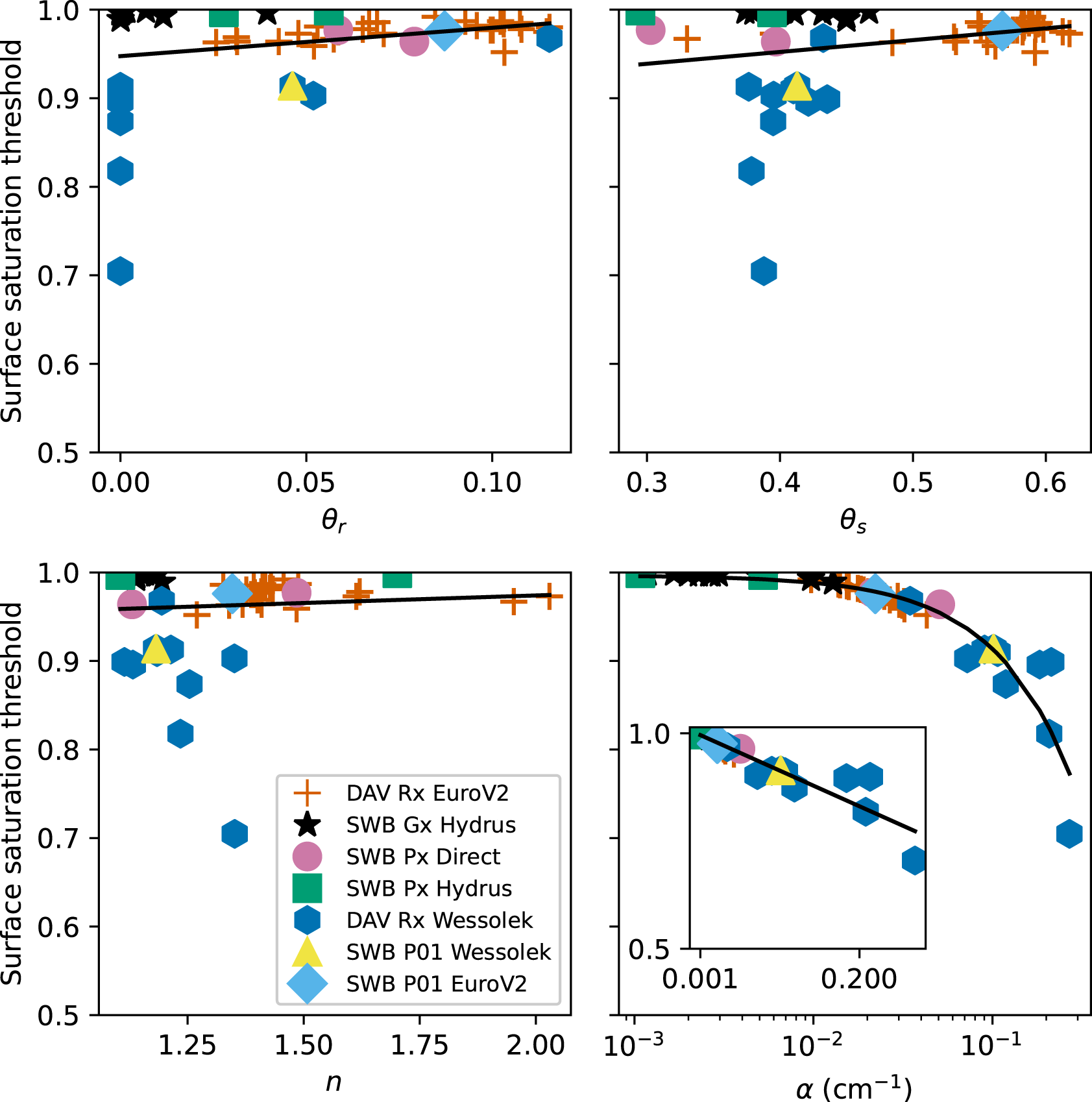
Figure 8. Dependence of the surface saturation threshold (SST) with each van Genuchten parameter using the reference snow. The black lines are linear fits that show a strong correlation between α and the SST, and weak correlations between SST and the other van Genuchten parameters. The inset in the plot for α has the same x and y bounds as the main plot, but with a linear x-scaling.
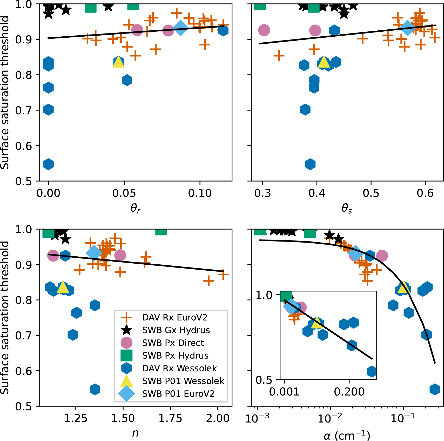
Figure 9. Dependence of the surface saturation threshold (SST) with each van Genuchten parameter using the maximum  $\rho/d$ (density/grain diameter) ratio ( $1.2 \times 10^{-6}\ \mathrm{kg\ m}^{-4}$) snow. The black lines are linear fits that show a strong correlation between α and the SST, and weak correlations between SST and the other van Genuchten parameters. The inset in the plot for α has the same x and y bounds as the main plot, but with a linear x-scaling.
The Hydrus and direct fitting methods resulted in different van Genuchten parameter values for Seewer Berg profiles (SWB Px) with differences in both α and n (Fig. 10). The PTFs also resulted in different van Genuchten parameter values for SWB P01, with small variations only for  $\theta_{\mathrm{r}}$.
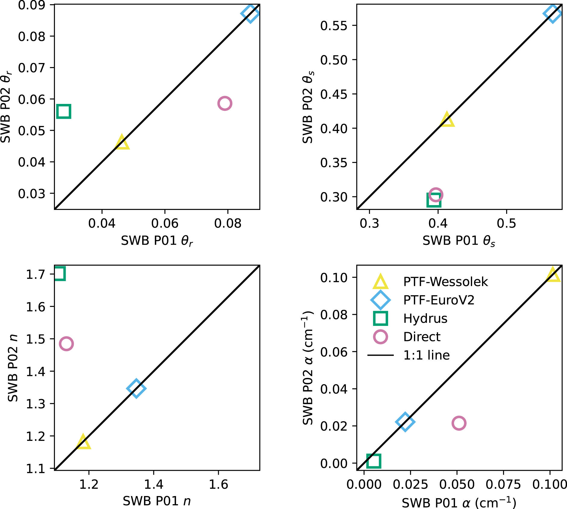
Figure 10. Comparison of van Genuchten parameters for the Seewer Berg profiles (SWB P01 and SWB P02). Points farther from the 1:1 line indicate greater differences between the profiles, while points closer to the 1:1 line indicate more similarity. The PTFs correspond only to SWB P01 since texture and density were only measured at SWB P01 and are plotted on the 1:1 line for reference.
3.5. Field measurements
The Seewer Berg grid sensors (SWB Gx) measured daily LWC values between 0.22 and 0.46 in the three winters presented here (Fig. 11). This corresponded to a range of saturation values between 0.55 and 1.11, which were defined using the maximum measured daily LWC during the fitting period as  $\theta_{\mathrm{s}}$. Saturation values above 1 are not realistic and indicate a discrepancy in the definition of $\theta_{\mathrm{s}}$ (maximum value between May and September 2023) and the measured values in the other time windows (see Discussion). In 2021/22, SWB G01 was the only sensor to exceed a saturation of 1 until the second half of March when four other sensors also slightly exceeded 1. In 2022/23, only SWB G01 exceeded a saturation of 1. In 2023/24, sensors SWB G02, G04 and G05 briefly exceeded a saturation of 1.
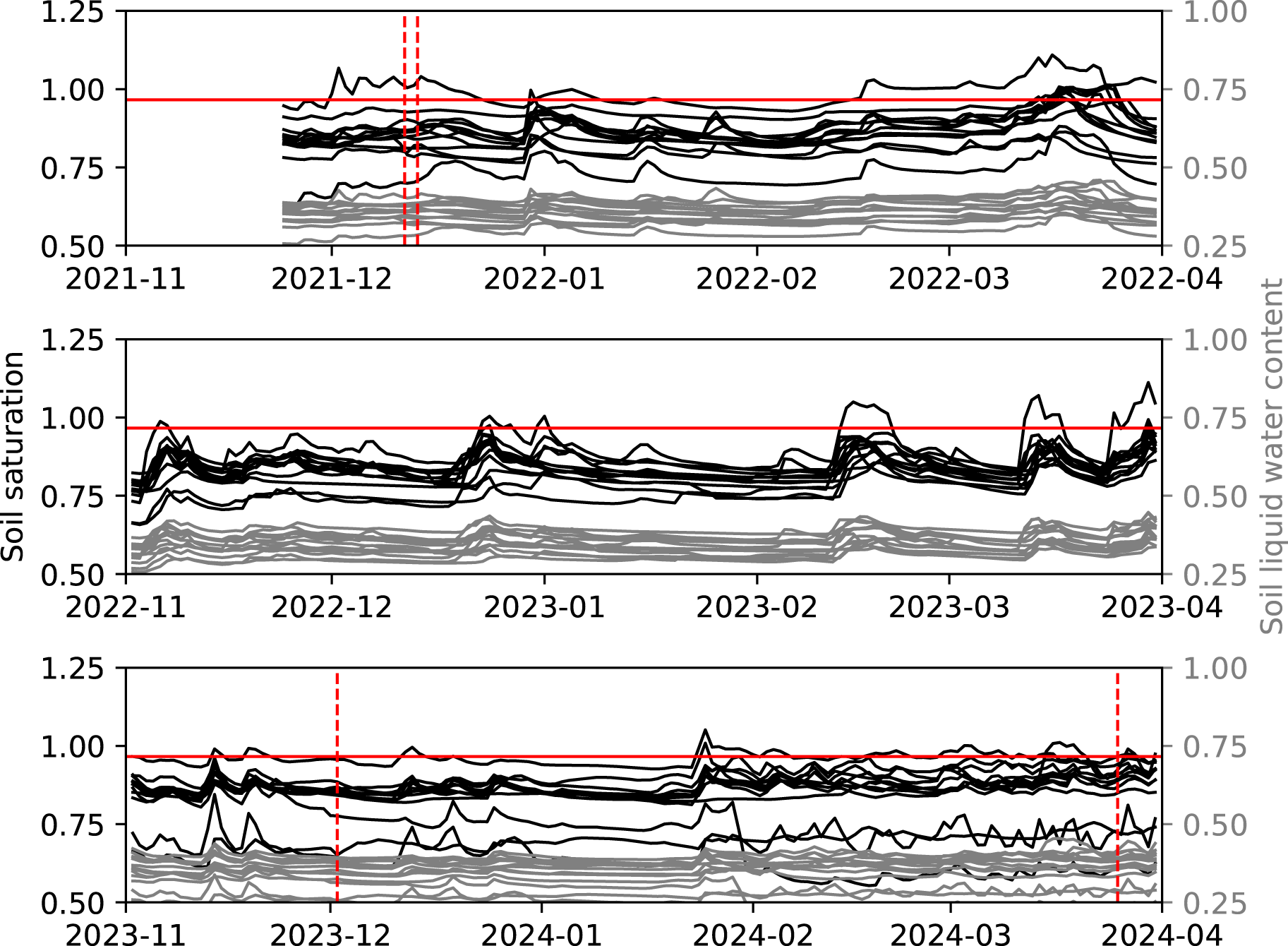
Figure 11. Time series of the daily LWC (gray) and saturation (black) of the 13 Seewer Berg grid sensors (SWB Gx) for three winters. Saturation was calculated as the effective saturation according to Eqn (3) where  $\theta_{\mathrm{s}}$ was set as the maximum daily LWC during the fitting period, 1 May–30 September 2023. The vertical dashed red lines indicate when avalanches classified as interface events (when capillary rise is thought to be relevant) released on the Seewer Berg. The horizontal solid red line marks a soil saturation of 96.6%, which corresponds to the boundary curve of the reference soil and snow at 5 cm soil depth (equal to sensor depth).
The LWC measurements in the soil showed an average daily range of 0.11, 0.10 and 0.15 in 2021/22, 2022/23 and 2023/24, respectively (Fig. 11), where the average daily range is the range of measured LWC values each day, averaged over the fitting period. Average daily saturation ranges were 0.26, 0.15 and 0.33 for 2021/22, 2022/23 and 2023/24, respectively. Thus, the sensor grid was the most homogeneous in 2022/23 and the least homogeneous in 2023/24.
When the SST of 91.5% from the reference snow and soil is adjusted for the 5 cm sensor depth, a saturation of 96.6% is required at 5 cm depth to allow for capillary suction. This threshold was exceeded for 7.5%, 1.9% and 3.6% of the measurements for 2021/22, 2022/23 and 2023/24, respectively. Some of the measurements that exceeded the threshold were from the aforementioned sensors with ill-defined  $\theta_{\mathrm{s}}$ values.
The field measurements were analyzed for four avalanches (11 December 2021, 13 December 2021, 02 December 2023, 25 March 2024) classified as ‘interface events’ (red dashed lines in Fig. 11). Avalanches were classified as interface events by Fees and others (Reference Fees, van Herwijnen, Altenbach, Lombardo and Schweizer2025) when the snowpack model indicated that liquid water could not have reached the ground from the snow surface. This condition is fulfilled when there is no surface melting or rain at the snow surface, or when the snowpack is cold enough that small amounts of surface melt cannot percolate to the ground. Thus, interface events are interesting as capillary suction is a plausible mechanism for the formation of wet basal layers during these events. For the four interface events analyzed, the saturation threshold of 96.6% was only exceeded by a single sensor at the time of release for the 11 December 2021, 13 December 2021 and 02 December 2023 avalanches (always the sensor with ill-defined  $\theta_{\mathrm{s}}$), and by no sensor for the 25 March 2024 avalanche.
When considering the maximum  $\rho/d$, the required saturation at 5 cm drops to 86.8% and was exceeded by 43.0%, 25.7% and 50.7% of the measurements in 2021/22, 2022/23 and 2023/24, respectively. This threshold was exceeded by five sensors for each of the avalanches in 2021/22, by three sensors for the 02 December 2023 avalanche and by nine sensors for the 25 March 2024 avalanche.
No avalanches were recorded in the 2022/23 winter and little snowfall during this winter led to frequent snow-free conditions on Seewer Berg.
4. Discussion
4.1. Suction envelope assumptions
The suction envelope shows the conditions under which capillary suction from the soil into the snow could occur and the resulting LWC of the basal snow. However, the results must be interpreted considering the assumptions of the calculation. One assumption is that the suction envelope represents the equilibrium condition and ignores all dynamic factors such as vapor transport, snow metamorphism and heat transfer. For example, temperature gradients in soils have been shown to cause liquid and vapor transport, with the cold side of the gradient having an increased LWC (Morel-Seytoux and Peck, Reference Morel-Seytoux and Peck1981). This effect has been shown to increase the LWC near the soil surface under a snow cover and during cold periods (Rollins, Reference Rollins1954; Joshua and Jong, Reference Joshua and Jong1973; Iwata and others, Reference Iwata, Hayashi, Suzuki, Hirota and Hasegawa2010). Temperature gradients with positive soil temperatures could also cause melting of the basal snow layers, which would increase the amount of available water for capillary suction. This is known as geothermal melting and is a separate mechanism for interfacial water formation (e.g. McClung and Clarke, Reference McClung and Clarke1987; Simenhois and Birkeland, Reference Simenhois and Birkeland2010).
Perhaps the most important factor that was not accounted for was snow metamorphism. Snow is known to undergo grain rounding and coarsening when wet (Wakahama, Reference Wakahama1974; Colbeck, Reference Colbeck1975; Raymond and Tusima, Reference Raymond and Tusima1979; Brun, Reference Brun1989), where the rate of metamorphism is proportional to LWC (Brun, Reference Brun1989). This grain coarsening decreases  $\rho/d$ and therefore also the amount of capillary suction. Since the profiles were taken several days before and after avalanche release, the true conditions at the time of release are unknown. We assumed that the true conditions were somewhere between the minimum and maximum $\rho/d$ values, and hopefully, near the average. More frequent profiles and/or snowpack modeling may be useful for determining the basal snow conditions at the time of release.
The calculation also assumed that the soil, vegetation and snow are hydraulically connected. Field observations on Seewer Berg show that the grass under the snowpack tends to be wet during most of the winter, which would suggest that the three materials are hydraulically connected. Glide-snow avalanches also occur on other substrates such as rock slabs (Clarke and McClung, Reference Clarke and McClung1999), shrubs (Kawashima and others, Reference Kawashima, Iyobe, Matsumoto and Greene2016) and bamboo (Endo, Reference Endo1985), which are less likely to allow for capillary suction. Rock slabs are frequently impermeable, while shrubs and bamboo can form thick interfaces (tens of centimeters) with large voids that are less likely to retain a hydraulic connection between the soil and snow. For sites in colder climates with shallow snowpacks, capillary suction may also be completely inhibited or delayed due to the presence of frozen soil layers or refreeze upon contact with a cold snowpack (Iwata and others, Reference Iwata, Hayashi, Suzuki, Hirota and Hasegawa2010; Watanabe and others, Reference Watanabe, Kito, Dun, Wu, Greer and Flury2013).
Finally, the soil was treated as a homogeneous layer. Because all of the measurements (LWC, matric potential, soil texture) used here were taken at depths between 0 cm and 10 cm, this assumption seems reasonable. When considering measurements deeper in the soil, these layers would need to be incorporated into the calculation and, for example, the Hydrus simulations.
While these assumptions are certainly a simplification of real conditions, the calculation still provides an estimation of the theoretical amount of capillary suction and allows for the calculation of capillary suction based on field measurements. Because the suction envelope depends on both the soil and snow properties, variations in both materials need to be considered.
4.2. Snow properties
Capillary suction was shown to increase with increasing snow density and decreasing grain diameter. This dependence is due to the parameterization by Yamaguchi and others (Reference Yamaguchi, Watanabe, Katsushima, Sato and Kumakura2012), which uses the  $\rho/d$ ratio to estimate the α and n parameters of the van Genuchten model. α is a scaling parameter that shifts the WRC, while n is related to the width of the pore-size distribution and affects the slope of the WRC (van Lier and Pinheiro, Reference van Lier and Pinheiro2018). This means that α has a dominant effect on the SST and maximum soil depth (Fig. 5), while n predominantly affects the shape of the LWC profile within the snow (Fig. 4).
Smaller n values result in more gradual changes of LWC with height, while larger n values cause a more rapid change. In Fig. 4, we see rapid changes from saturated to dry conditions over ∼5 cm height, which is consistent with high n materials such as coarse sands (Benson and others, Reference Benson, Chiang, Chalermyanont and Sawangsuriya2014). For the average and maximum  $\rho/d$, n was 8.06 and 14.79, respectively. This means that small changes in the matric potential (a few centimeters of pressure) can lead to large changes in the basal LWC and LWC profile.
The rapid transition from saturated to dry conditions makes the estimation of the α parameter very important. The α parameter controls the height of this transition and can be compared to the air-entry value (as 1/α) (van Lier and Pinheiro, Reference van Lier and Pinheiro2018), also referred to as the capillary rise height or the height of the capillary fringe. Here, the α values of the parameterization by Yamaguchi and others (Reference Yamaguchi, Watanabe, Katsushima, Sato and Kumakura2012) were adjusted by a factor of 1.4 to retrieve the wetting curve based on reported hysteresis (Adachi and others, Reference Adachi, Yamaguchi, Ozeki and Kose2020; Leroux and others, Reference Leroux, Marsh and Pomeroy2020). For the minimum, average and maximum  $\rho/d$ ratios, the air-entry values are 2.5 cm, 5.0 cm and 14.7 cm, respectively. These values are consistent with the reported values of capillary rise by Jordan (Reference Jordan1995) (1.5–8.75 cm) and the height of the saturated capillary fringe by Coléou and Lesaffre (Reference Coléou and Lesaffre1998) (1.5–11 cm). The accuracy of measurement techniques used to determine snow density and grain diameter are therefore very important.
Density measurements are relatively consistent, with errors of ∼10% between various methods (Proksch and others, Reference Proksch, Rutter, Fierz and Schneebeli2016; Hao and others, Reference Hao, Mind’je, Feng and Li2021). Grain size measurements, on the other hand, are extremely variable due to the number of techniques and differences in how grain size is defined. While an comparison of the many techniques (e.g. Baunach and others, Reference Baunach, Fierz, Satyawali and Schneebeli2001; Fierz and others, Reference Fierz, Armstrong, Durand, Etchevers, Greene, McClung, Nishimura, Satyawali and Sokratov2009; Yamaguchi and others, Reference Yamaguchi, Watanabe, Katsushima, Sato and Kumakura2012; Leppänen and others, Reference Leppanen, Kontu, Vehvilainen, Lemmetyinen and Pulliainen2015) is outside the scope of this paper, we address a few practical points. The traditional method for grain size estimation in the field is typically performed with a crystal card and magnifying glass and results in a subjective range from the average grain size to the average maximum grain size (Fierz and others, Reference Fierz, Armstrong, Durand, Etchevers, Greene, McClung, Nishimura, Satyawali and Sokratov2009). However, the parameterization by Yamaguchi and others (Reference Yamaguchi, Watanabe, Katsushima, Sato and Kumakura2012) is based on a more quantitative approach using microscope photographs of individual grains with automatic area measurements. This means it is difficult to compare the results of studies that used different grain size measurement methods. In any case, determination of the grain size is extremely important and an improved parameterization based on more quantitative values such as specific surface area (Legagneux and others, Reference Legagneux, Cabanes and Dominé2002) may be necessary to improve descriptions of the WRC for snow.
4.3. Limitations of the soil characterization methods
In addition to the effects of the snow properties discussed above, the van Genuchten parameter values of the soils also affect the suction envelope (Fig. 6). The differences are due to the methods used to determine the van Genuchten parameter values as well as the physical properties of the soils themselves (e.g. pore size distribution). The PTFs use physical information such as soil texture and density to predict the van Genuchten parameter values, while the Hydrus and direct fitting methods only use LWC and matric potential measurements. Thus, the PTFs depend on the data upon which they are based, while the fitting methods depend on the soil moisture measurements.
For the 25 Davos region soils (DAV Rx), the same variations in soil texture led to larger variations of the boundary curves for the Wessolek PTF compared to the EuroV2 PTF (Fig. 6). The Wessolek PTF is therefore more sensitive to soil texture. However, the intra-PTF variations were smaller than the inter-PTF differences (Cornelis and others, Reference Cornelis, Ronsyn, Van Meirvenne and Hartmann2001), demonstrating the importance of selecting an appropriate PTF. Since no PTF for alpine soils exists, other methods, such as the fitting methods used here, for retrieving the van Genuchten parameter values may be more appropriate.
We can compare the PTFs to the fitting methods for SWB P01, since all four methods were used for this soil. The Wessolek PTF resulted in the lowest SST, followed by the direct fitting, EuroV2 PTF and Hydrus fitting (Fig. 7). This order can be explained with the α parameter values (Fig. 10) and is consistent with the correlation between α and the SST. If we consider the fitting methods as ground truth, the EuroV2 PTF seemed to perform better than the Wessolek PTF for SWB P01 and may be more representative of this soil. Additional data are necessary to make more generalized statements about existing PTFs and their applicability to alpine soils.
For the fitting methods themselves, we see good agreement between the methods (Figs. 6 and 7). Specifically, the Hydrus method resulted in relatively low α values. The low α values correspond to large capillary forces (high suction) within the soil and therefore simply inhibit any significant capillary suction into the snow. The direct fitting method resulted in larger α values and therefore more capillary suction.
In addition to the aforementioned differences between the fitting methods, each method also has a few noteworthy limitations. For example, as stated above, the fitting methods are limited by the field data and are only able to provide accurate values for  $\theta_{\mathrm{r}}$ and $\theta_{\mathrm{s}}$ when sufficiently wet and dry conditions are achieved. This can be problematic because some tensiometers dry out before measuring the dry end of the WRC (e.g.
Wicki and others, Reference Wicki, Halter and Stähli2024) while other matric potential sensors are unreliable close to saturation. For the Seewer Berg profiles (SWB Px), matric potential values down to −1 hPa (manufacturer minimum measurable value) were measured. We therefore assume that saturated or nearly saturated conditions were correctly detected. However, as seen in the field data, quantification of
$\theta_{\mathrm{s}}$ when sufficiently wet and dry conditions are achieved. This can be problematic because some tensiometers dry out before measuring the dry end of the WRC (e.g.
Wicki and others, Reference Wicki, Halter and Stähli2024) while other matric potential sensors are unreliable close to saturation. For the Seewer Berg profiles (SWB Px), matric potential values down to −1 hPa (manufacturer minimum measurable value) were measured. We therefore assume that saturated or nearly saturated conditions were correctly detected. However, as seen in the field data, quantification of  $\theta_{\mathrm{s}}$ was challenging for the Seewer Berg grid sensors (SWB Gx) and was due to the use of a single fitting period. The use of a single and short fitting period is problematic because field measurements of LWC and matric potential are known to show seasonal variations (Fu and others, Reference Fu, Liao, Chai, Li and Lv2021; Aqel and others, Reference Aqel, Reusser, Margreth, Carminati and Lehmann2024) and to change year-over-year due to structural variations (Hannes and others, Reference Hannes, Wollschläger, Wöhling and Vogel2016; Sourbeer and Loheide II, Reference Sourbeer and Loheide2016; Fu and others, Reference Fu, Liao, Chai, Li and Lv2021). Thus, the fitting methods could be improved with an increased frequency of fitting.
Field measurements are also known to be highly hysteretic (Hannes and others, Reference Hannes, Wollschläger, Wöhling and Vogel2016). Hysteresis was addressed for the direct fitting of the Seewer Berg profiles (SWB Px) by averaging and geometrically binning the LWC vs matric potential curves prior to fitting. This allowed for an estimation of the drainage curve and provided a more accurate estimation of  $\theta_{\mathrm{s}}$, since fitting to the raw, unbinned data tended to reduce $\theta_{\mathrm{s}}$. Hysteresis was also an issue for the inverse solution method with Hydrus. Including hysteresis in the solver can improve results but also adds complexity by introducing additional parameters to describe both the wetting and drying curves. For simplicity, the fits performed for the Seewer Berg grid sensors (SWB Gx) were done without hysteresis.
The inverse fitting with Hydrus also has a few other limitations. For example, the method is limited by the need for accurate precipitation and evaporation data as well as, optionally, root water uptake, which was not used here. This means the method requires a nearby weather station. Another issue with the inverse fitting was that not all of the Seewer Berg grid sensors (SWB Gx) could be successfully fit (13 of 22). The sensors that could not be fit did not react at all, only very little, or delayed to precipitation events. These sensors may be installed in a location where precipitation does not reach the soil due to structural barriers such as vegetation or large macropores that transport most of the water around the sensors. Dynamic fitting of these sensors is then not appropriate. Finally, the inverse fitting is dependent on the initial values for the fitting parameters. This means that the results are not necessarily unique and there is no guarantee that the true best fit has been achieved.
4.4. Spatial variability
While the soil characterization techniques were responsible for significant differences in the suction envelopes, the spatial variability of the soil is also important. Spatial variability in soils is well-known and has been reported as variations between sensors at 1 m spacing (Bauser and others, Reference Bauser, Kim, Ng, Bugaj and Troch2022) and as correlation lengths down to 0.15 m (Deurer and others, Reference Deurer, Duijnisveld and Böttcher2000). This is supported by the differences in the measured LWC values between SWB P01 and P02 (Appendix), which are only 1.5 m apart. The differences in measured LWC resulted in different van Genuchten parameter values (Fig. 10), but only marginal differences between the direct fitting boundary curves (Fig. 7). The differences in the measured LWC could be due to many parameters including BD (Cai and others, Reference Cai, Zhou and Sheng2013), skeleton fraction (Arias and others, Reference Arias, Virto, Enrique, Bescansa, Walton and Wendroth2019; Naseri and others, Reference Naseri, Iden, Richter and Durner2019) or root network (Lu and others, Reference Lu, Zhang, Werner, Li, Jiang and Tan2020). For example, Seewer Berg is known to contain multiple types of grasses and shrubs (Feistl and others, Reference Feistl, Bebi, Dreier, Hanewinkel and Bartelt2014) and local differences in how the vegetation was disturbed and regrew could have led to differences between the two profiles. Alternatively, the differences could be related to the use of a single matric potential sensor applied to both LWC sensors. The relationship between the soil conditions at the matric potential measurement may be more or less representative of the conditions at each of the LWC sensors. Ideally, paired LWC and matric potential sensors would be distributed in a grid like the SWB Gx sensors, to allow for spatio-temporal measurements and quantification of the WRC.
In addition to the spatial variability of the soil, the variability of snow must also be considered. Correlation lengths of various snow properties have been reported down to 0.5 m (Schweizer and others, Reference Schweizer, Kronholm, Jamieson and Birkeland2008; Meloche and others, Reference Meloche, Gauthier and Langlois2024). Thus, it appears that the relevant length scale for fully describing capillary suction across the soil–snow interface is on the order of centimeters to 1 m. Recent finding on Seewer Berg indicate that the spatial correlation of the soil LWC in the week prior to avalanche release varied between about 12 m and 21 m (Fees and others (Reference Fees, Lombardo, van Herwijnen, Lehmann and Schweizer2024a); submitted). While noticeably larger than the aforementioned 1 m length scale, the correlation lengths may have been limited by the 8 m sensor spacing.
4.5. Capillary suction conditions on Seewer Berg
The required saturation at 5 cm depth for the reference soil was 96.6% with reference snow (average  $\rho/d$ ratio) and 86.8% with the maximum $\rho/d$ ratio. The results showed that significantly more sensors exceeded the saturation threshold when using the maximum compared to the average ratio. In order to determine the $\rho/d$ ratios for each avalanche, we used the lower value in the reported range of grain size as this has been shown to be more representative of the average determined through objective imaging techniques (Baunach and others, Reference Baunach, Fierz, Satyawali and Schneebeli2001). The two avalanches in December 2021 had $\rho/d$ ratios in a profile prior to avalanche release of $1.2 \times 10^{-6}\ \mathrm{kg\ m}^{-4}$ (i.e. the maximum $\rho/d$). Thus, considering the representative soil, 5 of the 13 Seewer Berg grid sensors (SWB Gx) were within the suction envelope in the days preceding the avalanche releases (snow profile taken 3 and 5 days prior to release, respectively). For the 02 December 2023 avalanche, the $\rho/d$ ratio was $0.4 \times 10^{-6}\ \mathrm{kg\ m}^{-4}$ (i.e. the average $\rho/d$) and suggests that only 1 of the 13 sensors were within the suction envelope (snow profile take 4 days prior to release). For the 25 March 2024 avalanche, a $\rho/d$ ratio of $0.6\ \times\ 10^{-6}\ \mathrm{kg\ m}^{-4}$ was measured 17 days prior to avalanche release. Since this was so long before avalanche release, we also consider the profile taken 1 day after the avalanche, which resulted in a $\rho/d$ of $0.9 \times 10^{-6}\ \mathrm{kg\ m}^{-4}$. These values fall between the average and maximum $\rho/d$ and indicate that up to nine sensors could have been within the suction envelope. Because only 13 of the 22 grid sensors could be fit with the Hydrus method, it is difficult to make conclusive statements about the fraction of the slope that was within the suction envelope for a given event. However, the snow in early winter tended to have higher $\rho/d$ ratios, supporting the idea that capillary suction is relevant for interface events in early winter (Fees and others, Reference Fees, van Herwijnen, Altenbach, Lombardo and Schweizer2025).
For the 2021 and 2023 avalanches, Fees and others (Reference Fees, Lombardo, van Herwijnen, Lehmann and Schweizer2024a) showed an increased LWC within the snow at a height of 5 cm. These data are reproduced in Figs. 12 and 13 with the Seewer Berg profile sensors (SWB Px), which were the closest soil sensors. The snow LWC sensor was not operational for the 2024 avalanche and this avalanche was therefore not included here. While the snow LWC increased prior to the 2021 and 2023 avalanche releases, Fig. 14 shows that both soil sensors were outside of the suction envelope for all three events, even when considering the maximum  $\rho/d$ ratio. Thus, the data suggest that capillary suction of water out of the soil was unlikely for these avalanches. Instead, the increase in snow LWC was more likely due to capillary rise of water generated from melting of the basal snow layers by the warm soil (Fees and others, Reference Fees, Lombardo, van Herwijnen, Lehmann and Schweizer2024a). We cannot, however, completely rule out capillary suction from the soil due to the spatial variability of the soil and snow properties, as well as the uncertainties in estimating the van Genuchten parameter values. In any case, the snow LWC sensor curves in Figs. 12 and 13 likely show how the LWC within the snow responds to capillary rise, regardless of whether the water originates from within the soil or the snow.
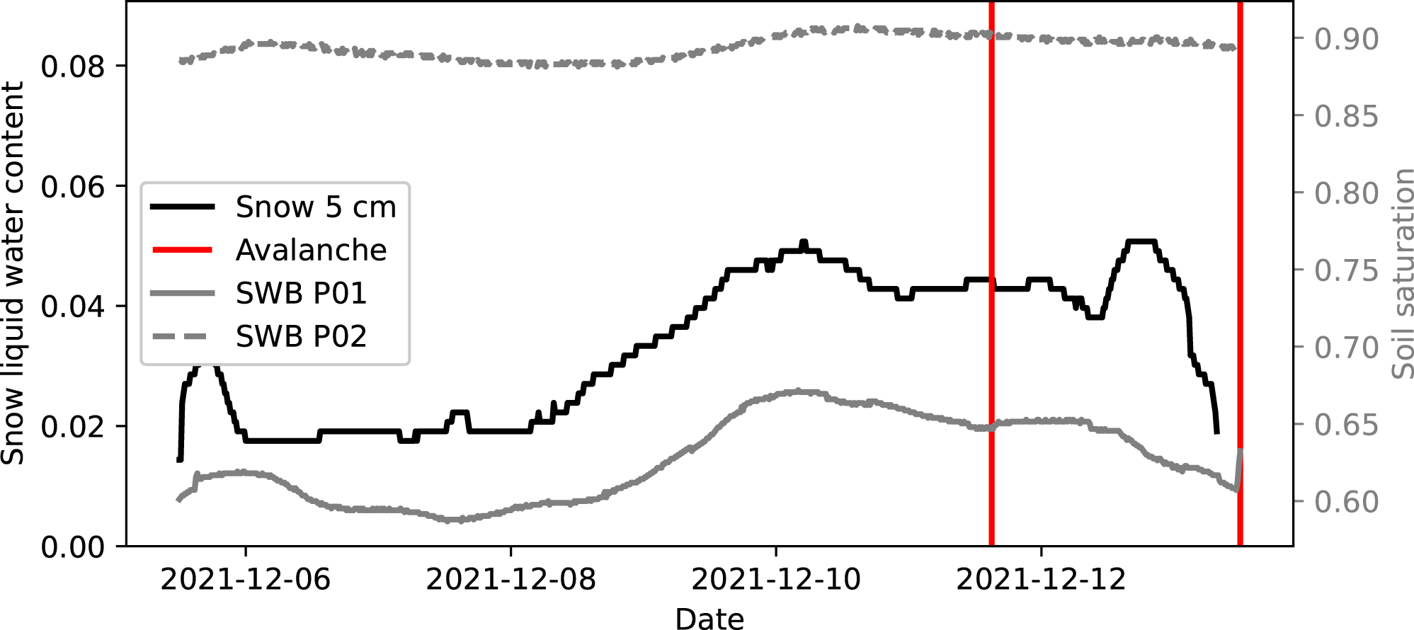
Figure 12. Time series of liquid water content measurements of the snow sensor at a height of 5 cm and the Seewer Berg soil profile sensors (SWB P01 and P02) for the two avalanches in December 2021 (red lines). The liquid water content of the soil sensors is displayed as soil saturation using the same method used for the grid sensors (SWB Gx). The vertical lines indicate the estimated avalanche release time (+/− 1 hour).
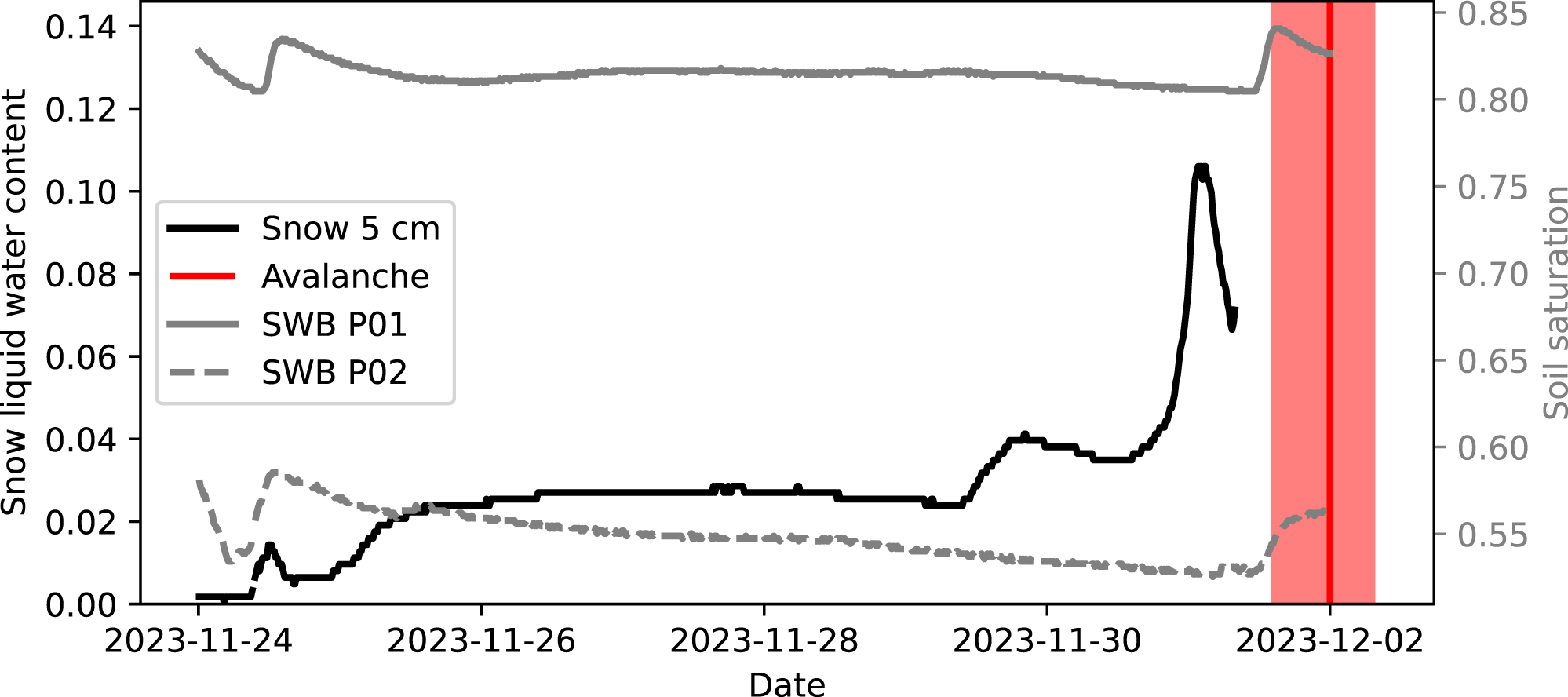
Figure 13. Time series of liquid water content measurements of the snow sensor at a height of 5 cm and the Seewer Berg soil profile sensors (SWB P01 and P02) for the avalanche in December 2023. The liquid water content of the soil sensors is displayed as soil saturation using the same method used for the grid sensors (SWB Gx). The vertical line indicates the estimated avalanche release time with the shading indicating the uncertainty since the avalanche released during a period of poor visibility.
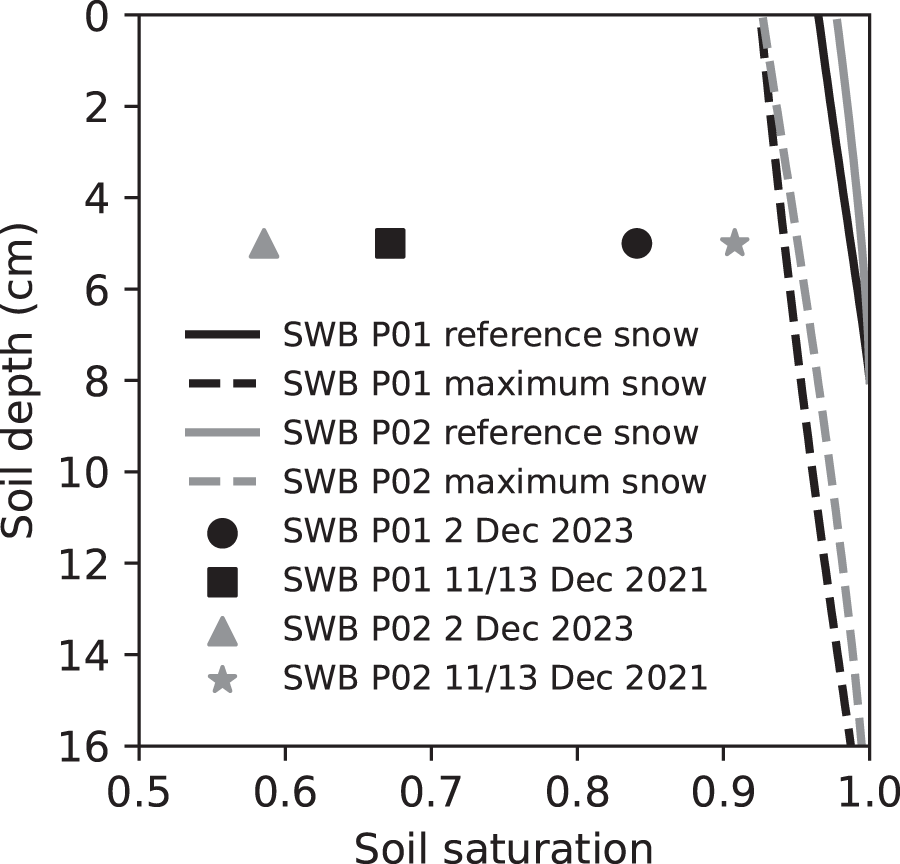
Figure 14. Lines representing the boundary curves of the suction envelopes for the Seewer Berg soil profiles (SWB P01 and P02) considering both the reference snow ( $\rho/d=0.2\times10^{6}\ \mathrm{kg\ m}^{-4}$) and maximum $\rho/d$ ratio ( $\rho/d=1.2\times10^{6}\ \mathrm{kg\ m}^{-4}$). The points indicate the maximum soil saturation in the time period prior to avalanche release (Figs. 12 and 13).
Another factor that influences the fraction of the Seewer Berg slope within the suction envelope is the threshold for capillary suction. All calculations presented here were done with an increase in LWC of 0.5% above  $\theta_{\mathrm{r}}$. However if a LWC larger than 0.5% above $\theta_{\mathrm{r}}$ is necessary, the boundary curves will shift to higher values. Recent results by Fees and others (Reference Fees, Lombardo, van Herwijnen, Lehmann and Schweizer2024a) suggest that the threshold may be around 3% LWC for interface events. Thus, even higher soil saturation values than those presented here may be needed to generate sufficient water in the basal snow for avalanche release.
5. Conclusions and outlook
We investigated capillary suction as a mechanism for the formation of wet basal snow layers at the soil–snow interface for gliding snow and glide-snow avalanches as proposed by Mitterer and Schweizer (Reference Mitterer and Schweizer2012). The suction envelopes for 40 alpine soils in Davos, Switzerland were calculated using field measurements of LWC, matric potential and soil texture data.
The results showed that capillary suction of water across the soil–snow interface is possible under certain conditions but generally requires a high soil saturation near the soil surface. The necessary surface soil saturation of 91.5% for the reference soil and snow used here was rarely achieved for the interface events on Seewer Berg. Thus, it is unlikely that capillary suction contributed significant amounts of interfacial water for these avalanches. Instead, other mechanisms for interfacial water formation such as geothermal melting were likely responsible (Fees and others, Reference Fees, Lombardo, van Herwijnen, Lehmann and Schweizer2024a).
The results also showed that capillary forces of both the soil and snow are important for determining the conditions under which capillary suction could occur. Namely, that soils with low capillary forces (high α values) allow for more capillary suction, while snow with high capillary forces (low α values; high density and small grain diameter) increases capillary suction.
These results have several implications for future investigations of glide-snow avalanches. First, while capillary suction does not seem to be a dominant mechanism for the formation of wet basal layers on Seewer Berg, the result could be highly site specific and additional data are needed to make more general conclusions. For scenarios where capillary suction does occur, the capillary rise is limited to about 10 cm for realistic snow properties, which should be considered with respect to effects on the mechanical properties of snow and proposed release mechanisms (McClung, Reference McClung1981; McClung and Clarke, Reference McClung and Clarke1987; Bartelt and Lehning, Reference Bartelt and Lehning2002). The theoretical results of this study should be verified with laboratory experiments or controlled field measurements in the future to confirm that the suction envelope accurately predicts conditions with capillary flow into the basal snow layers.
Second, considering the high spatial variability of soil and snow properties, in-situ monitoring is likely the only method capable of providing the necessary spatial and temporal resolution for studying water formation at the soil–snow interface (e.g. Fees and others, Reference Fees, Lombardo, van Herwijnen, Lehmann and Schweizer2024a). This means that the common practice of using a reference location outside of the gliding slope is likely insufficient. Field studies on glide-snow avalanches should therefore focus on glide-snow avalanches that release in a similar location year after year (e.g. Humstad and others, Reference Humstad, Venås, Dahle, Orset and Skrede2016), so that the slope can be well instrumented. Since spatially resolved snow profiling is difficult within the active slope due to safety considerations and disturbance of the snowpack, snowpack modeling (e.g. Lehning and others, Reference Lehning, Bartelt, Brown and Fierz2002a; Reference Lehning, Bartelt, Brown, Fierz and Satyawali2002b) will likely need to be incorporated. Advances in remote sensing (e.g. radar) may also eventually allow for detection of the LWC spatial heterogeneity at the soil–snow interface (Vuyovich and others, Reference Vuyovich, Jacobs, Hiemstra and Deeb2017; Naderpour and chwank, Reference Naderpour and Schwank2018).
Finally, an improved description of the WRC for snow, covering the full range of naturally occurring grain types (or ideally objective parameters such as specific surface area) and densities, would be of great value. Capillary forces of snow are relevant not only for capillary suction at the soil–snow interface but also for snowpack drainage (Lombardo and others, Reference Lombardo, Lehmann, Kaestner, Fees, Van Herwijnen and Schweizer2025), capillary barriers within the snowpack (Avanzi and others, Reference Avanzi, Hirashima, Yamaguchi, Katsushima and De Michele2016) and capillary rise of brine on sea ice (Domine and others, Reference Domine, Sparapani, Ianniello and Beine2004; Wever and others, Reference Wever, Rossmann, Maaß, Leonard, Kaleschke, Nicolaus and Lehning2020).
In summary, capillary suction across the soil–snow interface can introduce water into the basal snowpack under certain conditions. Additional investigations are needed to understand the interplay between capillary suction, other mechanisms for interfacial water formation and the mechanisms for glide-snow avalanche release.
Data availability statement
The full soil dataset used here including coordinates, LWC, matric potential, texture and density is available on EnviDat (https://www.doi.org/10.16904/envidat.571).
Acknowledgements
This project was funded by SNSF Grant 200021-212949.
Competing interests
The authors declare no competing interests.
Appendix
SWB P01 and P02 fits
The LWC and matric potential measurements for SWB P01 (Fig. A1) and SWB P02 (Fig. A2) were averaged (daily), geometrically binned and fit to Eqn (2).
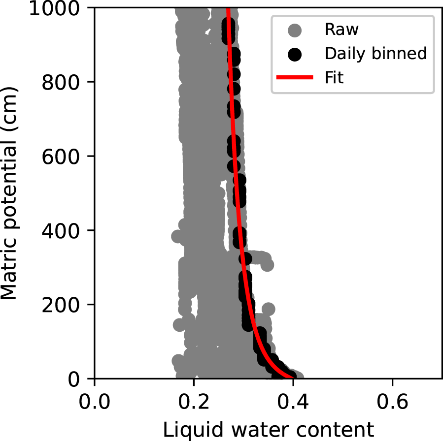
Figure A1. Fit for SWB P01. Raw data are at 15 min resolution.
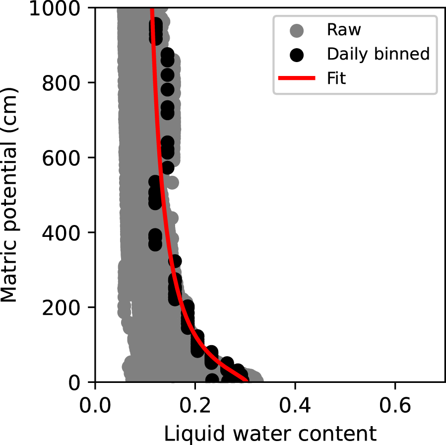
Figure A2. Fit for SWB P02. Raw data are at 15 min resolution.
Suction envelope calculation
To calculate the suction envelope, the matric potential of the soil ( $h_{\mathrm{soil}}$) is first determined using Eqn (2) and the van Genuchten parameter values for the soil as
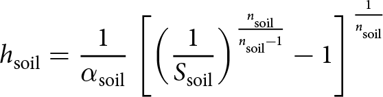 \begin{equation}
h_{\mathrm{soil}} = \frac{1}{\alpha_{\mathrm{soil}}}
\left[
\left(\frac{1}{S_{\mathrm{soil}}}
\right)^{{\frac{n_{_{\mathrm{soil}}}}{n_{_\mathrm{soil}}-1}}}-1\right]^{\frac{1}{n_{_{\mathrm{soil}}}}}
\end{equation}
\begin{equation}
h_{\mathrm{soil}} = \frac{1}{\alpha_{\mathrm{soil}}}
\left[
\left(\frac{1}{S_{\mathrm{soil}}}
\right)^{{\frac{n_{_{\mathrm{soil}}}}{n_{_\mathrm{soil}}-1}}}-1\right]^{\frac{1}{n_{_{\mathrm{soil}}}}}
\end{equation} with soil saturation ( $S_{\mathrm{soil}}$) and soil depth ( $z_{\mathrm{soil}}$). The matric potential of the snow is then given by
 \begin{equation}
h_{\mathrm{snow}} = h_{\mathrm{soil}} + z_{\mathrm{soil}} + z_{\mathrm{interface}}
\end{equation}
\begin{equation}
h_{\mathrm{snow}} = h_{\mathrm{soil}} + z_{\mathrm{soil}} + z_{\mathrm{interface}}
\end{equation} where  $z_{\mathrm{interface}}$ is the thickness of the vegetation layer. Since the suction envelope is defined by the LWC of the basal snow, we only consider values of $h_{\mathrm{snow}}$ that satisfy Eqn (A.3) (same as Eqn (4) in the main text)
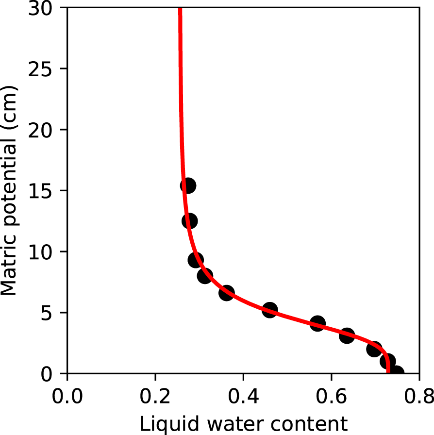
Figure A3. Measured and fit water retention curve for a grass sample from Seewer Berg.
 \begin{equation}
h_{\mathrm{snow}} \leq \frac{1}{\alpha_{\mathrm{snow}}}
\left[
\left(
\frac{\Delta\theta_{\mathrm{snow}}}{\theta_{\mathrm{s,snow}}-\theta_{\mathrm{r,snow}}}\right)^{-{\frac{n_{_{\mathrm{snow}}}}{n_{_{\mathrm{snow}}}-1}}}-1\right]^{\frac{1}{n_{_{\mathrm{snow}}}}}
\end{equation}
\begin{equation}
h_{\mathrm{snow}} \leq \frac{1}{\alpha_{\mathrm{snow}}}
\left[
\left(
\frac{\Delta\theta_{\mathrm{snow}}}{\theta_{\mathrm{s,snow}}-\theta_{\mathrm{r,snow}}}\right)^{-{\frac{n_{_{\mathrm{snow}}}}{n_{_{\mathrm{snow}}}-1}}}-1\right]^{\frac{1}{n_{_{\mathrm{snow}}}}}
\end{equation} where  $\Delta\theta_{\mathrm{snow}}$ is the capillary suction threshold (here, 0.5%). The values of $h_{\mathrm{snow}}$ from Eqn (A.3) that satisfy Eqn (A.3) are then substituted into Eqn (2) with the snow van Genuchten parameter values to obtain the snow LWC
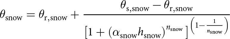 \begin{equation}
\theta_{\mathrm{snow}} = \theta_{\mathrm{r,snow}} + \frac{\theta_{\mathrm{s,snow}} - \theta_{\mathrm{r,snow}}}{\big[ 1 + \left( \alpha_{\mathrm{snow}} h_{\mathrm{snow}} \right)^{n_{\mathrm{snow}}} \big]^{\left(1-\frac{1}{n_{\mathrm{snow}}}\right)}}
\end{equation}
\begin{equation}
\theta_{\mathrm{snow}} = \theta_{\mathrm{r,snow}} + \frac{\theta_{\mathrm{s,snow}} - \theta_{\mathrm{r,snow}}}{\big[ 1 + \left( \alpha_{\mathrm{snow}} h_{\mathrm{snow}} \right)^{n_{\mathrm{snow}}} \big]^{\left(1-\frac{1}{n_{\mathrm{snow}}}\right)}}
\end{equation} and the suction envelope. This is repeated for each point ( $h_{\mathrm{soil}}$, $z_{\mathrm{soil}}$) to generate the entire suction envelope.
Grass WRC
Grass samples were taken from Seewer Berg near the SWB P01 soil profile. This grass was layered into a cylinder and compressed with a weight corresponding to the pressure of a 1 m snowpack (density  $400\ \mathrm{kg\ m}^{-3}$). This cylinder was connected to a water reservoir and the WRC was measured by measuring the change in mass as the water level was lowered.


 Open access