Extreme melt events on northern James Ross Island, Antarctic Peninsula region, linked to isentropic drawdown and Foehn winds

Abstract

The Antarctic Peninsula (AP) and James Ross Island (JRI) region have experienced exceptionally warm spells in recent decades, leading to substantial glacier mass loss. This study investigates a sequence of three massive heat waves between November 2022 and January 2023, leading to extreme surface ablation. Their impact was examined through a wide range of in-situ atmospheric and glaciological observations on two JRI glaciers: the cirque-based Triangular Glacier and the dome-shaped Davies Dome. Furthermore, the Weather Research and Forecasting model was used with a very-high horizontal resolution of 300 m to provide insights into surface–atmosphere interactions and the synoptic- and meso-scale drivers of the exceptionally high near-surface air temperatures. The three investigated events generated total surface ablation of 1237 mm w.e. on Triangular Glacier and 271 mm w.e. on Davies Dome contributing to annual ablation ≥4 times higher than a recent mean on Triangular Glacier. A striking local variability in atmosphere–glacier energy exchange was found in the complicated topography of the northeastern AP region. A complex foehn mechanism analysis revealed that isentropic drawdown with a small contribution of latent heat release played a crucial role in enhancing leeward warming and surface melt.

1. Introduction

The Antarctic Peninsula (AP) region is known for high climate variability, recent atmospheric warming and consequences related to the cryosphere. In the late 20th century, rapid warming was reported at many AP locations (Vaughan and others, 2003). An increase in air temperature led to significant glacier area reduction and mass loss (Davies and others, 2012; Engel and others, 2012), as well as rapid disintegration of the A and B segments of the Larsen Ice Shelf (LIS) (Scambos and others, 2003). A short-term absence of warming or even occasional cooling was observed at some AP stations in the period 2000–2015 (Turner and others, 2016), together with corresponding cryospheric responses such as increased snow accumulation and positive glacier surface mass balance (Oliva and others, 2017). The cooler period has been subsided by a restored temperature increase and acceleration of glacier area loss in the most recent years (Carrasco and others, 2021).

The warming trend was amplified along the eastern AP coast by a significant (p < 0.01) increase in the Southern Annular Mode (SAM) index (1965–2000). This tendency resulted in strengthening westerlies and enhanced foehn-favouring conditions (Marshall and others, 2006; Orr and others, 2008). The foehn hypothesis was supported by a statistically significant relationship between increased foehn frequency and raised air temperature at the Matienzo station located between Larsen A and B embayments (Cape and others, 2015). It was concluded that foehn winds significantly contributed to the catastrophic collapse of the Larsen A and B Ice Shelves (Laffin and others, 2022).

The foehn conditions in the AP region are characterised by relatively strong northwestern winds, reduced relative humidity and air temperatures commonly exceeding 0°C (Cape and others, 2015). In the LIS area, foehn is most common in winter and early spring; however, it still occurs 30–60 h per month in summer (Wiesenekker and others, 2017). The foehn wind can induce intense surface melt driven by sensible heat flux even in winter. Kuipers Munneke and others, (2018) reported sensible heat flux values of up to 300 W m⁻² in May 2016 at the Cabinet Inlet on LIS.

Foehn-induced warming can be caused by multiple mechanisms, such as isentropic drawdown and latent heat release during ascent. Mechanical mixing and radiative heating can also play an important role in leeward warming (Elvidge and others, 2015). Depending on the properties of the incoming flow (particularly the static stability and wind speed), the foehn impact may either rapidly weaken with distance from a mountain range or spread hundreds of kilometres into the leeward region, of which LIS is a prime example (Elvidge and others, 2016b, King and others, 2017). The leeward air temperature and wind vector fields can feature a complex structure due to the presence of relatively cool and moist foehn jets, which were also documented over LIS (Elvidge and others, 2015). The leading driver of the LIS surface melt during foehn events could be sensible heat flux (in the case of strong wind and stably stratified flow) or shortwave radiation (under light wind and weakly stratified flow) (Elvidge and others, 2020).

In recent years, multiple extreme warm events have been documented in the northern and eastern AP regions. A record-breaking air temperature of 18.3°C was reported on 06 February 2020 at the Esperanza station near the northern tip of the AP. This event was driven by the advection of warm Pacific Ocean air towards the AP around a high-pressure centre near Patagonia. The large-scale advection was combined with foehn development in the northeastern AP region (Xu and others, 2021; González-Herrero and others, 2022). The following very-high air temperature of 15.5°C observed on 09 February 2020 at the Marambio station (∼100 km south of Esperanza) was also related to foehn development with significant warming contribution by the isentropic drawdown mechanism (Bae and others, 2022).

The next extreme heat wave reached the AP in February 2022, when a large amount of heat and moisture was transported to the Peninsula by an atmospheric river (Gorodetskaya and others, 2023). As a result, anomalously high air temperatures and specific humidities were observed throughout the troposphere on the South Shetland Islands. The near-surface air temperature at King Sejong (13.7°C) and Carlini (13.6°C) stations on King George Island and at Palmer (11.6°C) and Faraday–Vernadsky (12.7°C) stations in the western AP region reached record-breaking levels. This warm spell was accompanied by unusually high rainfall amounts and intense snow melt in both eastern and western AP regions. Foehn development enhanced the melt over the eastern AP due to increased sensible and shortwave radiation heat fluxes. However, the impact of foehn clearance (i.e. cloud cover reduction in the leeward region) was limited in places affected by strong and moist gap flows (Gorodetskaya and others, 2023; Zou and others, 2023).

This paper focuses on three of the most recent heat waves recorded at the northeastern AP, particularly on James Ross Island (JRI), between November 2022 and January 2023, which induced massive melt but have not yet been reported in the literature. Their impact on the boundary layer characteristics and the cryosphere is described using a wide range of atmospheric and glaciological observations from two JRI glaciers. Furthermore, numerical model output at a very high horizontal resolution is used to analyze the large- and meso-scale processes, leading to the observed intense snow melting and glacier ablation. Attention is given to the principal mechanisms of foehn winds, as well as foehn’s impact on surface energy fluxes. These results are compared with available AP–foehn-related papers focused mostly on the LIS. Finally, we assess the atmospheric and cryospheric findings within the regional context of northern AP changes.

2. Data and methods

2.1. Study area

This study focuses on the northern AP region, particularly selected JRI glaciers Figs. 1 and 2. The JRI is located in the northwestern part of the Weddell Sea, separated by the Prince Gustav Channel from the AP. Most of its surface is glaciated, while the northwestern part, the Ulu Peninsula, represents one of the largest ice-free areas in the AP region (312 km²) (Kavan and others, 2017). Within the ice-free zone, multiple small cirque, valley and dome glaciers are located, surrounded by a complex topography of mesas, valleys and an extensive lowland (the Abernethy Flats). This work focuses on the cirque Triangular Glacier, with an area of 0.524 km² and an altitudinal range of 104–329 m a.s.l. (Engel and others, 2023), and the dome-shaped Davies Dome glacier, with an area of 6.49 km² and an altitudinal range of 0–514 m a.s.l. (Engel and others, 2018). An impression and the locations of the glaciers within the AP and JRI contexts are given in Figs. 1 and 2.

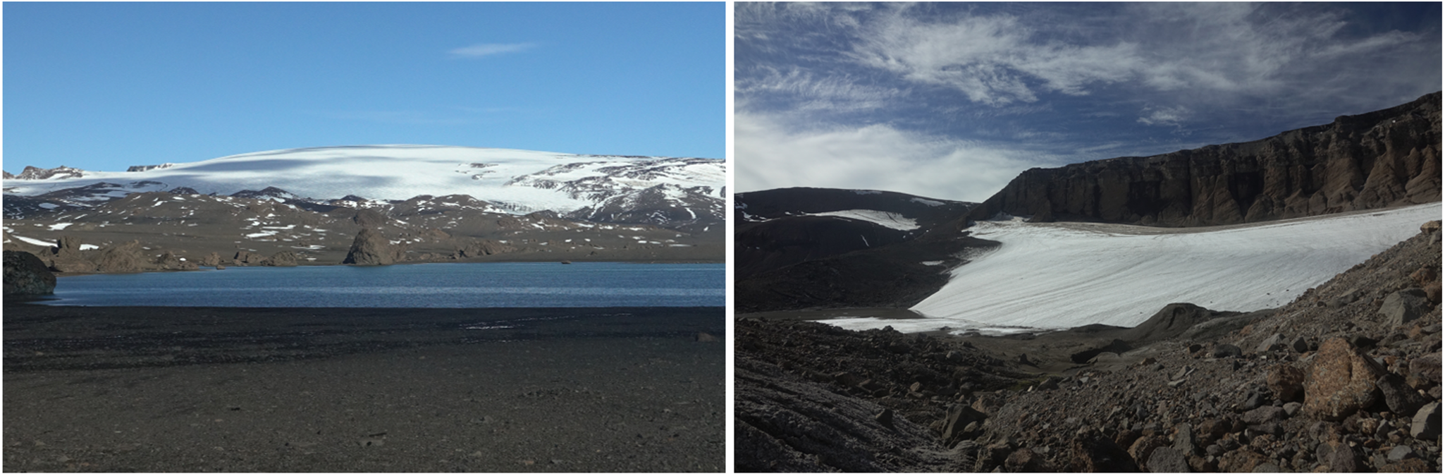
Figure 1. View on Davies Dome (left) and Triangular Glacier (right).

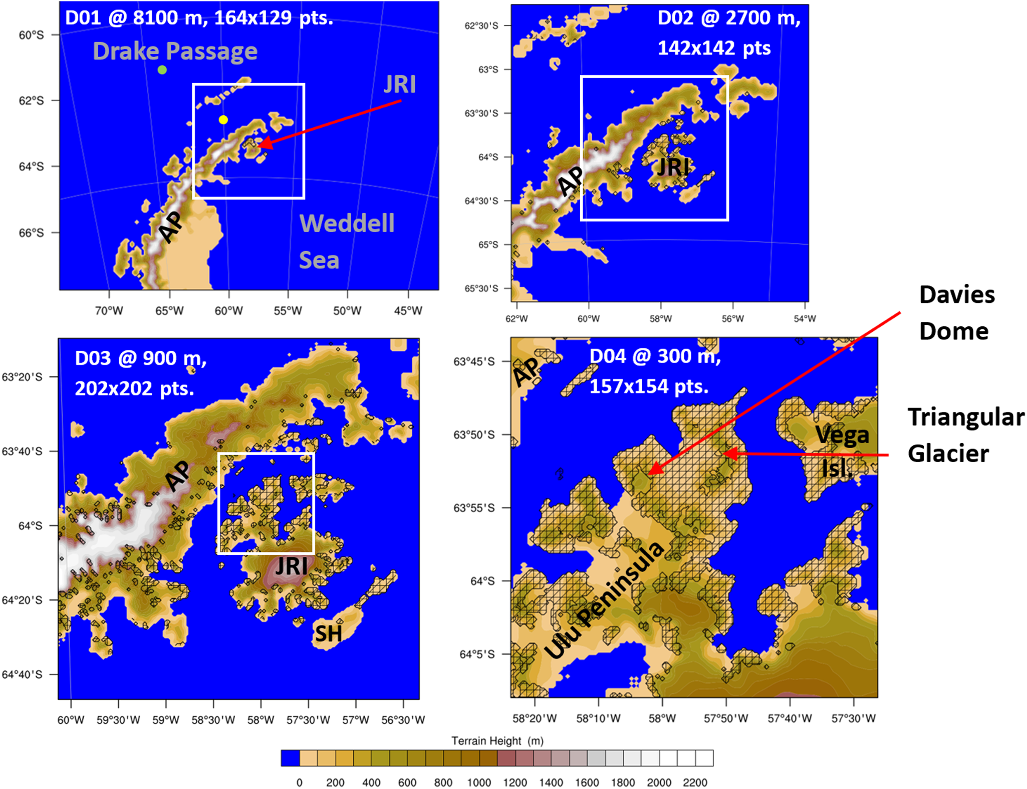
Figure 2. The WRF model domains D01–D04, their horizontal resolution and number of the WRF grid points. The geographical extent of the corresponding nested domains is indicated in the maps by the white rectangles. Ice-free areas are marked with a black grid. AP = Antarctic Peninsula, JRI = James Ross Island, SH = Snow Hill Island. The locations of air temperature vertical profiles (Figure 10) for open Southern Ocean and Bransfield Strait are shown in the D01 map by the green and yellow points, respectively.

2.2. In-situ observations

Both Davies Dome and Triangular Glacier are equipped with an automatic weather station (AWS) based on an EMS Brno V12 datalogger (Table 1). The Davies Dome AWS is located on the summit plateau of the dome-shaped glacier, while the Triangular Glacier AWS is placed in the central part of this glacier. The 2-m air temperature was observed using an EMS33H sensor with an accuracy of ±0.15°C. Wind speed was measured 2 m above the surface using a Young 05305 wind monitor (accuracy: ±0.2 m s⁻¹). The Triangular Glacier AWS was also equipped with a Kipp & Zonen NR-Lite 2 net radiometer.

Table 1. Geographical coordinates, physical and WRF model elevation of automatic weather stations (AWS) on Triangular Glacier and Davies Dome

Snow or ice surface height was observed at both AWSs using an ultrasonic distance sensor from Judd Communications, providing surface level data at 2-h (Davies Dome) and 4-h (Triangular Glacier) intervals. Snow water equivalent was calculated using snow density observations undertaken at both AWS sites in January and February 2022 (364.5 kg m⁻³ for Triangular Glacier and 360.6 kg m⁻³ for Davies Dome). For the Triangular Glacier, where the AWS is located below the recent equilibrium line altitude (ELA; Engel and others, 2023), a density of 900 kg m⁻³ was used for glacier ice. This density value was derived from earlier JRI glaciological studies (Engel and others, 2018, 2023).

2.3. Weather Research and Forecasting model configuration

The simulations were conducted using the Weather Research and Forecasting (WRF) model (Skamarock, 2019), version 4.3. Initial and boundary conditions for WRF simulations were derived from the ERA5 reanalysis (resolution of 0.25° × 0.25°) provided by ECMWF (Hersbach and others, 2020). A high-resolution (3.125 km) sea ice concentration dataset from the University of Bremen (Spreen and others, 2008) was included in the WRF lower boundary files to improve the representation of heat and moisture exchange at the ocean–atmosphere interface. Similarly, the default digital elevation model (DEM) was replaced by Reference Elevation Model of Antarctica, a highly detailed and accurate DEM (Howat and others, 2019). The land-cover grid was derived from the SCAR Antarctic Digital Database (British Antarctic Survey, 2018) and the topography map by the Czech Geological Survey (2009). Four one-way-nested domains were used to achieve 300-m horizontal resolution in the innermost domain (Fig. 2). The model was run with 65-eta levels while the lowest level was located at ∼7 m above the ground to represent boundary layer processes well.

The selection of physical parameterisations followed the results of the WRF model validation studies in the JRI region (Matějka and others, 2021; Matějka and Láska, 2022), particularly the 3D TKE boundary layer scheme was selected (Zhang and others, 2018). This scheme was designed to be also valid for simulations in hundreds-of-metres order, that is, the ‘grey zone’ between the validity of traditional boundary layer parameterisations and large eddy scale (Doubrawa and Muñoz-Esparza, 2020). A positive impact of the 3D TKE scheme is likely to be more significant on the cirque-confined Triangular Glacier than at the higher-elevated and windy areas as is the summit region of Davies Dome glacier (Matějka and Láska, 2022). A detailed model configuration is provided in the Supporting Material (Table S1).

2.4. WRF simulations layout and postprocessing

For model initialisation, a rather simple setup of snow initial conditions with 1000 mm w.e. of snow cover on the glaciers was used. An exception was the glaciated grid points north of 64°S and below 320 m a.s.l., where the observed snow height at the Triangular Glacier was used as the initial snow height. The altitude of 320 m was selected, as it equals the ELA at northern JRI (Engel and others, 2018), while the latitude limit was set to avoid snow height underestimation in the cooler southern sectors of the WRF domains. Before each analysed ablation period, the model was given at least 6 days for the spin-up of small- and meso-scale processes (Warner, 2010). After simulation completion, the 10-m simulated wind speed was recalculated at 2-m observation height using a logarithmic formula to ensure that simulated and observed wind speeds are for the same height above the surface (details are given in Matějka and Láska, 2022). Furthermore, as a part of the foehn mechanism analysis, the non-dimensional mountain height of the flow approaching the AP was computed as follows:

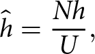\begin{equation*}\hat h = \frac{{Nh}}{U},\end{equation*}

where U is the upstream wind speed (in practice, averaged over a layer of an appropriate thickness considering obstacle height; see Elvidge and others, 2016b), N is the Brunt–Väisälä frequency, and h is the mountain height. The number ĥ describes the behaviour of the flow interacting with an obstacle. The value of ĥ <1 indicates a tendency towards the linear flow-over regime, while a value of ĥ >1 favours nonlinear phenomena, such as foehn winds (Lu and others, 2023), low-level blocking and leeside hydraulic jumps; a deeper theoretical context can thus be found (Orr and others, 2008; Elvidge and others, 2015).

2.5. Trajectory analysis

The Visualization and Analysis Platform for atmospheric, Oceanic, and solar Research v3.7.0 software (Li and others, 2019; Visualization & Analysis Systems Technologies, 2023) was used to compute backward trajectories of foehn wind using the WRF domain D03-based 3D wind fields. The trajectory computation was initiated over the northern part of JRI, covering both investigated glaciers (63.7732°S–63.8922°S; 57.7254°W–58.1362°W). Only trajectories overcoming the AP mountain range (i.e. reaching west of 59.4°W and north of 63.75°S) were selected to describe the foehn wind source region. The difference in trajectories’ altitude and air thermodynamical properties between the source region and leeward (foehn-affected) region contributed to the foehn mechanism analysis (Section 3.3).

2.6. Remote sensing imagery

To verify and support the WRF-based ablation maps, an analysis of snowmelt extent was conducted using available remote sensing images from the MODIS/Aqua Snow Cover Daily L3 Global 500 m SIN Grid product (Hall and Riggs, 2021). Due to cloud cover, only images with minimal cloud coverage between 15 and 28 December 2022, which cover the second warming period, were selected.

3. Results

3.1. Significant ablation events in the 2022/2023 summer on James Ross Island

Both Triangular Glacier and Davies Dome experienced significant surface ablation during the summer of 2022/2023 (Fig. 3). Between 01 November 2022, 20:00 UTC, and 16 January 2023, 00:00 UTC, total surface ablation on Triangular Glacier reached 1454 mm w.e., whereas 232 mm w.e. was observed on Davies Dome. After 16 January, the surface height data from Triangular Glacier ceased to be available due to the melting out of the sensor-mounting rod. There were three main periods (Fig. 3) of enhanced melt in late spring and the first half of the summer: 11–23 November 2022 (hereinafter Nov 22), 14–25 December 2022 (Dec 22) and 05–16 January 2023 (Jan 23) clearly separated by cooler periods with slow or absent surface ablation. From 01 February 2022, that is, from the beginning of the mass balance year (e.g. Engel and others, 2024), until sensor-mounting rod melt-out (16 January 2023), the surface lowering at Triangular Glacier AWS site reached 1614 mm w.e. It is highly probable that the surface ablation continued in the subsequent period until 01 February 2023, as the surface at the higher-elevated Davies Dome AWS lowered by 5 mm w.e. between 16 January 2023 and 01 February 2023. The surface mass loss at the Triangular Glacier AWS site was ≥4 times higher than the mean value in the 2014/15–2019/20 period, which was ∼400 mm w.e. y⁻¹ (Engel and others, 2023). At the Davies Dome AWS site, the surface mass loss between 01 February 2022 and 01 February 2023 was 270 mm w.e., while the mean mass balance in the 2009/10–2020/21 period was 0–100 mm w.e. y⁻¹ (Engel and others, 2024).

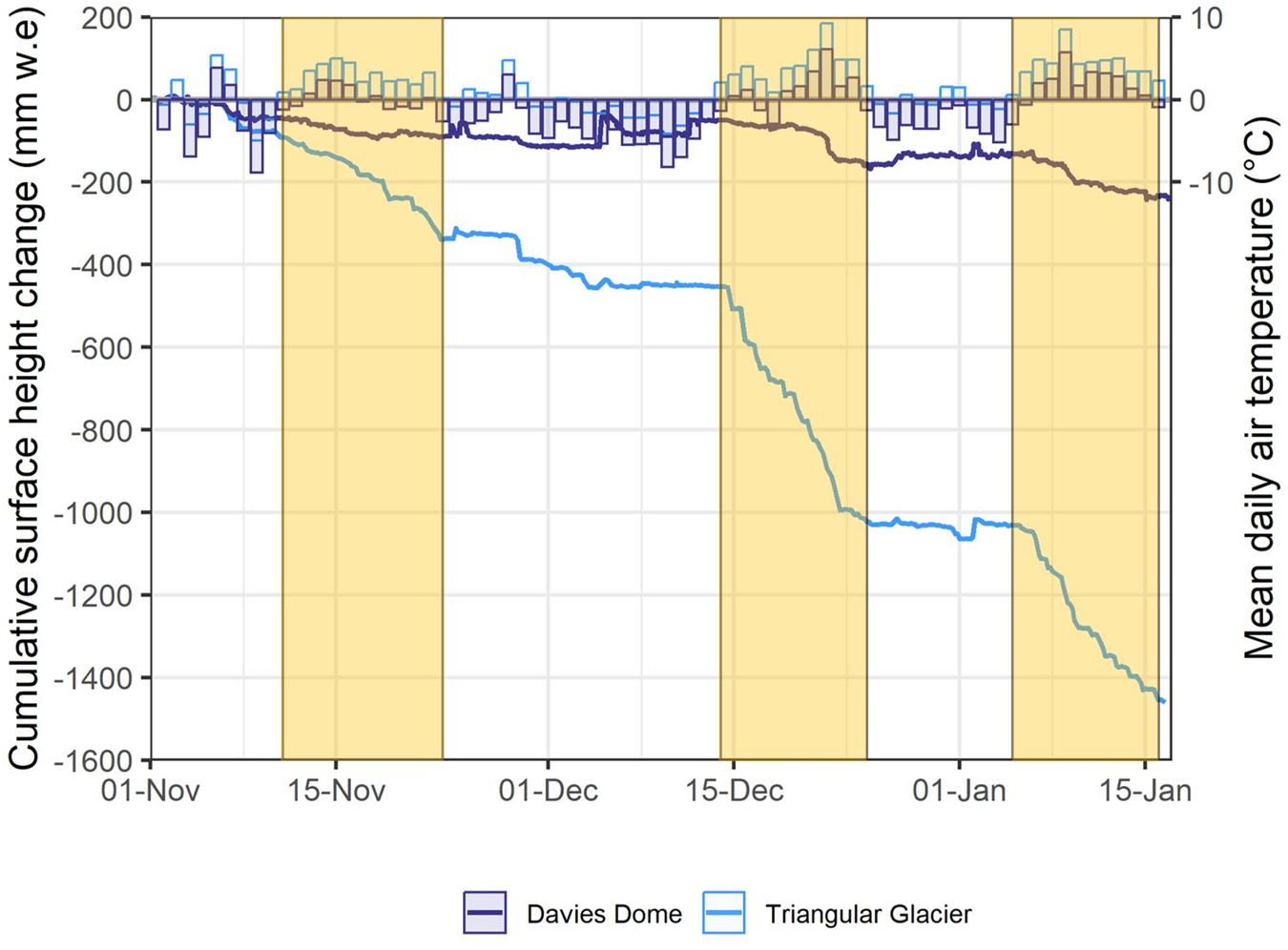
Figure 3. Cumulative surface height change in mm w. e. (solid line) and mean daily air temperature (bars) on Davies Dome and Triangular Glacier from 01 November 2022 00 UTC to 17 January 2023 00 UTC. Orange rectangles mark intense ablations periods.

The Nov 22 event was generally less intense than the Dec 22 and Jan 23 events. The mean melt intensity in the first event reached 0.86 mm w.e. h⁻¹ on Triangular Glacier and 0.16 mm w.e. h⁻¹ on Davies Dome, while it increased in the following events to 2.16 mm w.e. h⁻¹ (Dec 22) and 1.60 mm w.e. h⁻¹ (Jan 23) on Triangular Glacier and to 0.44 mm w.e. h⁻¹ (Dec 22) and 0.42 mm w.e. h⁻¹ (Jan 23) on Davies Dome. The lower ablation intensity in the Nov 22 event was accompanied by cooler conditions compared to the Dec 22 and Jan 23 periods (Table 2). The net radiation (i.e. the sum of shortwave [incoming and reflected] and longwave [emitted and received] radiation fluxes) measured on Triangular Glacier reached higher intensity in the Dec 22 (129.3 W m⁻²) and Jan 23 (103.5 W m⁻²) events compared to the Nov 22 event (81.4 W m⁻²).

Table 2. Summary of observed mean near-surface air temperature, wind speed, net radiation and surface melt rate during intense ablation events in summer 2022/2023 on Davies Dome (DD) and Triangular Glacier (TG). In addition, WRF-simulated mean surface energy fluxes (net radiation, sensible heat flux and latent heat flux) and total available energy for glacier mass warming or melting (i.e. the surface energy balance; SEB) is provided

Based on the WRF model output, the surface energy balance (SEB), that is, the sum of net radiation, sensible and latent heat fluxes, was positive in all events (Table 2). In this case it led to snow and glacier ice warming and melting, while a negative SEB would lead to snow and ice cooling and refreezing. This total flux into glacier surface was more intense on Triangular Glacier than on Davies Dome. Its highest values were simulated during the Dec 22 event, reaching 225.7 W m⁻² on Triangular Glacier and 74.1 W m⁻² on Davies Dome. The Jan 23 event was slightly less impactful in terms of the total energy input into the surface (by 12%–17%) while the Nov 22 event was markedly less intense on Triangular Glacier (with a mean value of 114.2 W m⁻²) and Davies Dome (with a mean value of 14.7 W m⁻²). In all events and on both glaciers, the positive SEB was driven by net radiation (30.9–149.0 W m⁻²) and sensible heat flux (39.7–99.3 W m⁻²) and partly compensated by the latent heat flux, that is, sublimation or evaporation (reaching between −55.9 and −22.7 W m⁻²).

3.2. The ablation event during 14–25 December 2022

3.2.1. In-situ meteorological conditions and surface energy fluxes

The main focus in this multi-scale analysis is the peak phase of the Dec 22 event. An identical examination of the Nov 22 and Jan 23 events revealed very similar results (albeit less pronounced during the Nov 22 event) and their description is therefore provided in the Supporting Material (Figs S1 to S8) to make this section easier to read. Note that the foehn mechanism analysis (Section 3.3) and the investigation of the regional context of surface heat fluxes and melting (Section 3.4) focus on all three events.

An unusually strong ablation event occurred on northern JRI on 14–25 December 2022, when highly favourable conditions led to extremely intense snow and ice melt. Based on the Judd sensor data, surface lowering on Triangular Glacier reached 568.4 mm w.e. in the event in total. A notable snow melt of 114.9 mm w.e. was also observed on Davies Dome. Exceptionally high air temperatures were recorded on 22 December 2022, reaching 9.5°C on Davies Dome and 12.1°C on Triangular Glacier (Fig. 4). On Davies Dome, the very high air temperature was accompanied by wind speed exceeding 20 m s⁻¹. High wind speed can be related to the exposed location of the dome-shaped glacier (in contrast to the rather confined location of Triangular Glacier).

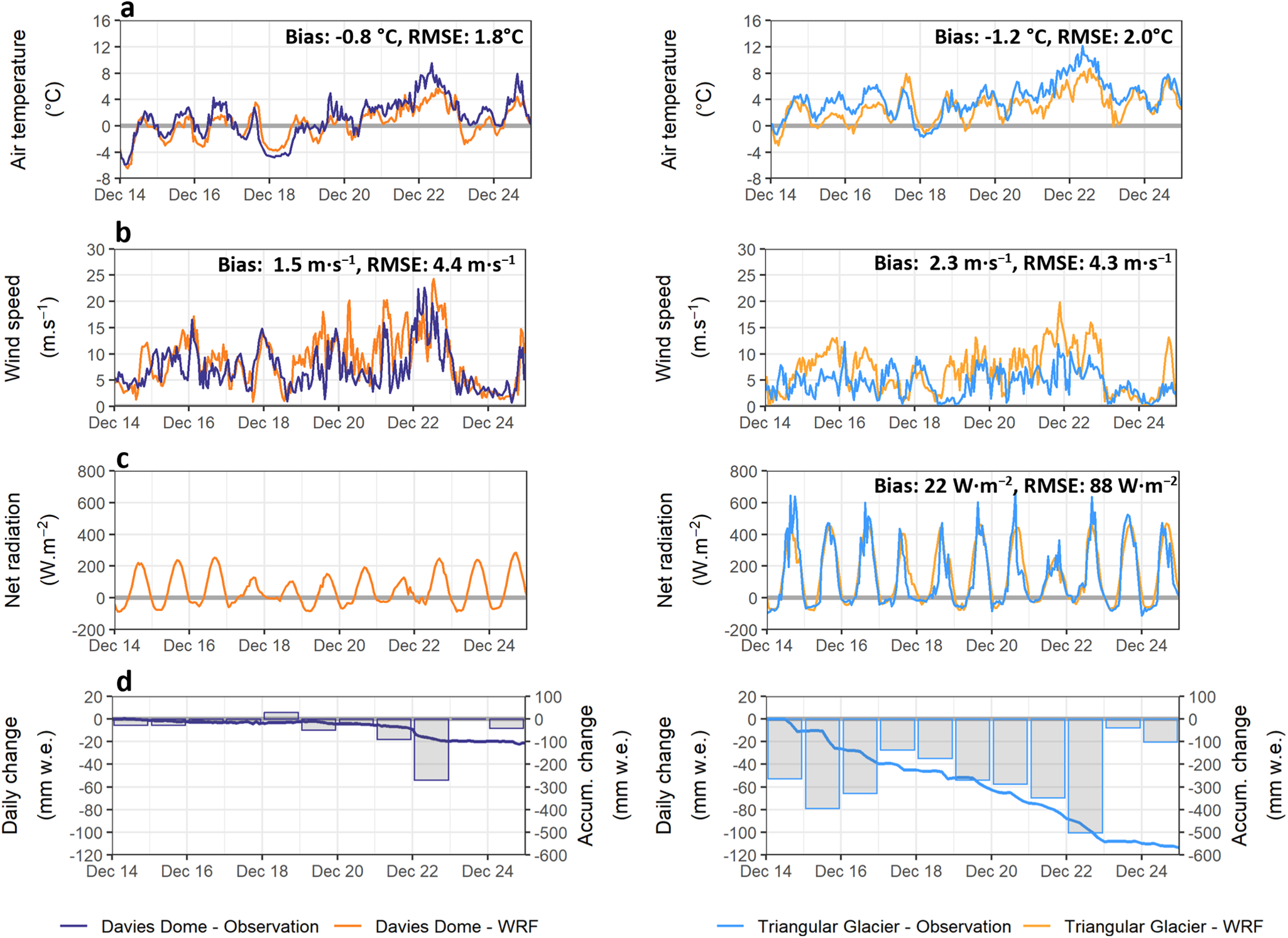
Figure 4. Observed and WRF-simulated near-surface meteorological parameters: air temperature (a), wind speed (b), net radiation (c), daily and accumulated surface height changes in mm w. e. (d), on Davies Dome (left) and Triangular Glacier (right) between 14 and 25 December 2022. Where available, the root-mean-squared error (RMSE) and bias of the WRF model are given in the plot.

The WRF-simulated mean net radiation flux during the event was positive and nearly three times higher on Triangular Glacier (149.0 W m⁻²) than on Davies Dome (53.4 W m⁻²). On Triangular Glacier WRF-based estimates of net radiation exceeded 400 W m⁻² in multiple days (the same is true for observations), while on Davies Dome, the modelled maximum value was 249 W m⁻² (net radiation observations were not available there). During the Dec 22 event, sensible heat flux contributed significantly to surface warming and glacier ablation with the mean WRF-simulated values between 58.8 W m⁻² on Davies Dome and 99.3 W m⁻² on Triangular Glacier.

Due to extremely high air temperatures and increased wind speed on 21–22 December, the WRF-based sensible heat flux reached highly elevated levels, peaking at >400 W m⁻² at both AWSs, while the latent heat flux was near zero or slightly positive (Fig. 5). Moreover, simulated positive net radiation (reaching up to >400 W m⁻² on Triangular Glacier and up to >200 W m⁻² on Davies Dome) further supported surface ablation. The combination of excessive turbulent and net radiation heat fluxes into the glacier surface on 22 December 2022 led to the highest observed daily ablation within all investigated periods. On Davies Dome, daily ablation reached an exceptionally high 53.8 mm w.e. (i.e. 19.9 mm w.e. more than the second highest recorded value within investigated events), while a daily rate of 100.4 mm w.e. was observed on Triangular Glacier.

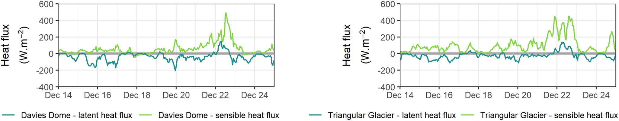
Figure 5. WRF-simulated sensible and latent heat fluxes on Davies Dome (left) and Triangular Glacier (right) between 14–25 December 2022.

3.2.2. Synoptic- and meso-scale processes leading to significant glacier ablation

The Dec 22 event culminated on 22 December 2022, at 08:00 UTC when the air temperature on Triangular Glacier reached 12.1°C. Prior to that, the northern AP was affected by strengthening warm-air advection from the northwest. The large-scale flow was driven by the pressure gradient between the Bellingshausen Sea Low and a high-pressure area placed northeasterly off the AP tip (Fig. 6). Later in the day of 22 December, cooler air from the west-southwestern direction started to be advected to the northern AP, and the air temperature on JRI glaciers began to decrease (Fig. 4a).

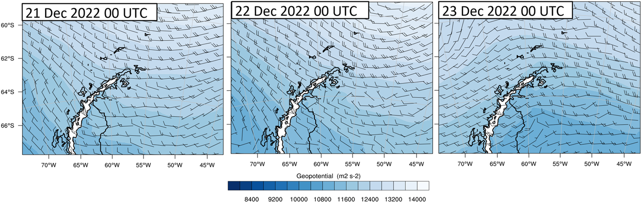
Figure 6. WRF-simulated 850-hPa wind vectors and geopotential over the Antarctic Peninsula region from 21 to 23 December 2022, always at 00:00 UTC.

Based on the WRF model output, the warming was amplified over the eastern AP region, including JRI, Vega Island and the surrounding Weddell Sea (Fig. 7a), indicating a potential foehn event. In the cross-sections perpendicular to the AP mountain range, further typical signs of foehn development could be observed (Figs. 7b, c), that is, isentropic drawdown leeward of AP and JRI (i.e. increase of air temperature in particular elevations), relative humidity decrease and fast downward motion followed by a development of mountain leeward waves. The air temperature in the foehn-affected area locally exceeded 10°C, whereas it remained close to 2°C over the sea to the west of the AP mountain range.

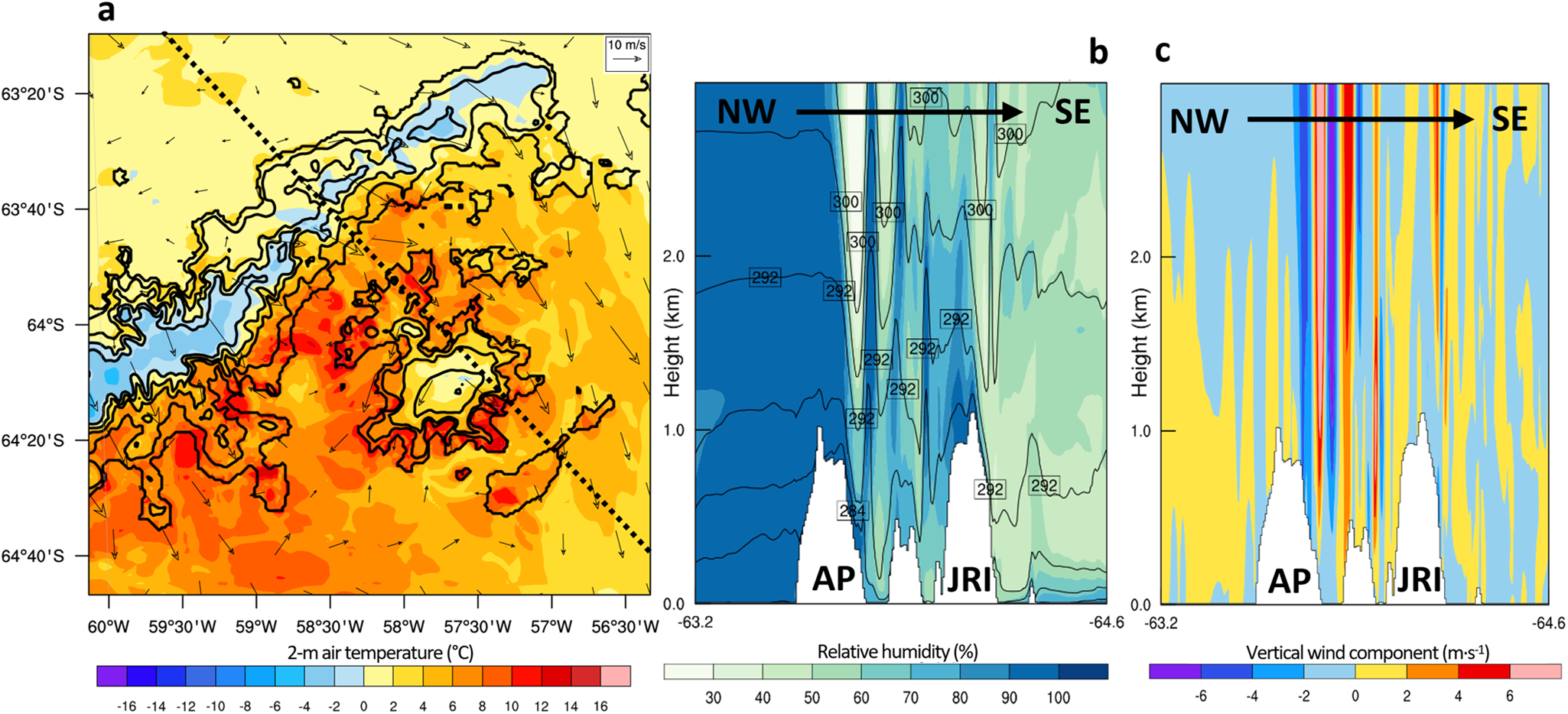
Figure 7. WRF-simulated 2-m air temperature (color), 10-m wind speed (arrows), and contours of model terrain at 400-m interval (black lines) in the northern Antarctic Peninsula region (a), vertical cross-sections of relative humidity and potential temperature in NW-SE direction (b), the same for vertical wind component (c). The position of the cross-section is shown as a dotted line in panel a. The horizontal arrows in the upper part of the cross-sections indicate the prevailing flow direction. The outputs are valid for the peak phase of the ablation event on 22 December 2022 at 08:00 UTC.

An analysis of the Nov 22 and Jan 23 events revealed that the foehn signature was very similar during the peak phase of the Jan 23 event (Fig. S8). The Nov 22 event also produced an isentropic drawdown and relative humidity drop while the leeward waves were less pronounced compared to the other two events (Fig. S6).

3.3. Foehn mechanisms analysis

Further insights into the processes driving and accompanying the three investigated foehn events were obtained through an investigation of moisture transport and precipitation (Section 3.3.1), analysis of vertical stratification of the air mass advected to the AP (Section 3.3.2) and, finally, a thorough examination of the vertical displacement of foehn trajectories and changes to their thermodynamical properties (Section 3.3.3).

3.3.1. Integrated water vapour transport and precipitation

Integrated water vapour transport (IVT) was analysed using the ERA5 data due to a limited spatial extent of the WRF model outermost domain D01. During the peak of the Nov 22 event, there was limited moisture transport towards the AP, while more intense transport was directed to the northwestern Drake Passage (Fig. 8a). The Dec 22 event was accompanied by a moderately intense atmospheric river related to the IVT values of ∼400 kg m⁻¹ s⁻¹ over the South Shetland Islands and the Bransfield Strait between these islands and the northwestern AP. During the Jan 23 event, a massive amount of moisture was transported towards the ocean east of the Tierra del Fuego, marginally also affecting the northern AP, where IVT values reached 100–300 kg m⁻¹ s⁻¹.

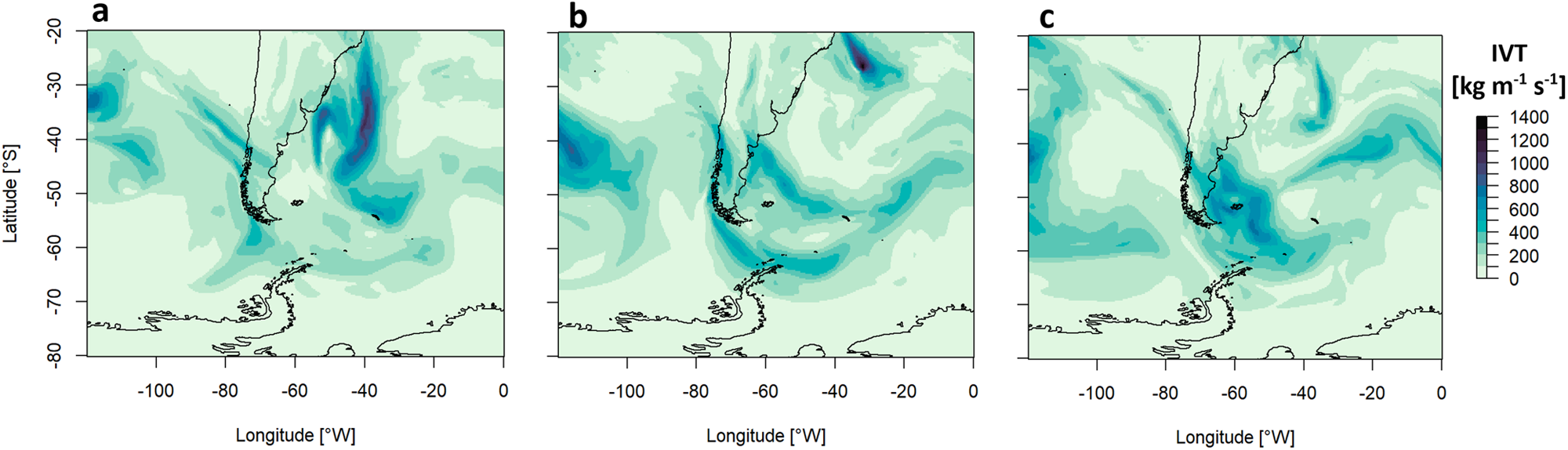
Figure 8. ERA5-based integrated water vapor transport (IVT; kg m⁻¹ s⁻¹) in the region defined by 20–80°S and 0–120°W on 15 November 2022 17:00 UTC (a), 22 December 2022 08:00 UTC (b), 09 January 2023 11:00 UTC (c).

To assess a potential role of precipitation-related leeward warming of the flow over the AP mountains, the 12-h precipitation sum from the WRF model was plotted (Fig. 9). The precipitation-related leeward warming can occur when the ascending flow is heated via condensation, then liquid water is removed by precipitation, and the drier descending air is warmed following the dry-adiabatic lapse rate (Elvidge and Renfrew, 2016a). The 12-h intervals symmetrically surrounded the peak phase of each foehn event (i.e. 15 November 2022 17:00 UTC, 22 December 2022 08:00 UTC, and 09 January 2023 11:00 UTC). During the Nov 22 event, precipitation occurred over most of the northern AP with ∼10–15 mm estimated windward (i.e. to the northwest) of the investigated northern JRI glaciers. Higher accumulation values within 15–25 mm were found over the higher mountains further south. Precipitation during the Dec 22 event was less evenly distributed, with ∼5 mm NW of the investigated glaciers but ∼40 mm (with localised sums >55 mm) over the more prominent AP mountains near 64° 10’S. The last event featured a very similar pattern to the Dec 22 event. Precipitation amount NW of the studied glaciers reached 5-10 mm while the sums over the mountains further south were slightly lower compared to the previous event. The events also differed by snowfall fraction on total precipitation. During the peak phase of the Nov 22 event, snowfall fraction (averaged over all D03 grid points) reached 60% while during the Dec 22 and Jan 23 events, the fraction decreased to only 27% and 45%, respectively, corresponding to higher air temperature in the windward region during the peak phase of the Dec 22 and Jan 23 events (Figs. 7a, S6a, S8a).

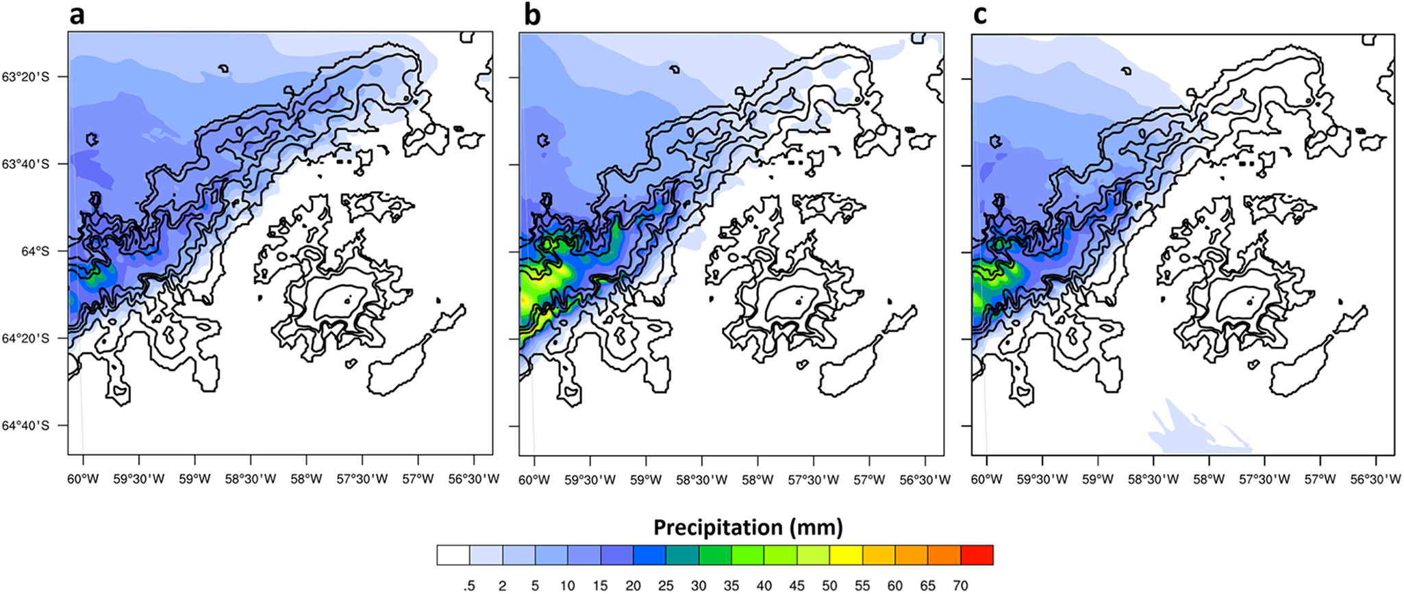
Figure 9. WRF-simulated precipitation over 12-h periods surrounding trajectory analysis times: 15 November 2022 11:00–23:00 UTC (a). 22 December 2022 02:00–14:00 UTC (b). 09 January 2023 05:00–17:00 UTC (c). The countour lines (black) are given at 400-m interval.

3.3.2. Vertical stratification of air mass advected to the Antarctic Peninsula

To evaluate the vertical structure of the air mass advected to the AP, WRF-based air temperature profiles between 200–1500 m a.s.l. were plotted (Fig. 10) over the open Southern Ocean NW of northern AP (61.5°S, 64.0°W) and over the Bransfield Strait (63.1°S, 60.0°W). Geographical context of both locations is shown in Figure 2. Note that the selected altitudinal range was similar to Elvidge and others (2015) while considering the lower crest altitude of northern AP mountains compared to the section adjacent to the Larsen C Ice Shelf. During the peak phase of the Nov 22 event, the lapse rate was relatively constant with a shallow stable layer near the bottom of the profile. In contrast, during the Dec 22 event, there was a rather deep very stable layer (with a lapse rate close to 0°C 100 m⁻¹) below 800 m a.s.l. at both investigated locations. An elevated inversion near 800 m a.s.l. (open ocean) and near 1000 m a.s.l. (Bransfield Strait) is the most striking feature of the Jan 23 profiles. Furthermore, the non-dimensional mountain height is shown. The ĥ values were 0.75 (Nov 22), 1.04 (Dec 22) and 1.07 (Jan 23) suggesting a tendency to linear flow-over regime (Nov 22) and borderline to blocking regime (Dec 22 and Jan 23). These relatively low values, considering the thermal stratification, can be explained by the rather high wind speed; mean values reached 16.3 m s⁻¹ (Nov 22), 18.3 m s⁻¹ (Dec 22) and 15.2 m s⁻¹ (Jan 23). Note, final flow regime could also be affected by the above-mentioned elevated stable layers within the incoming air mass (see discussion in Section 4.3).

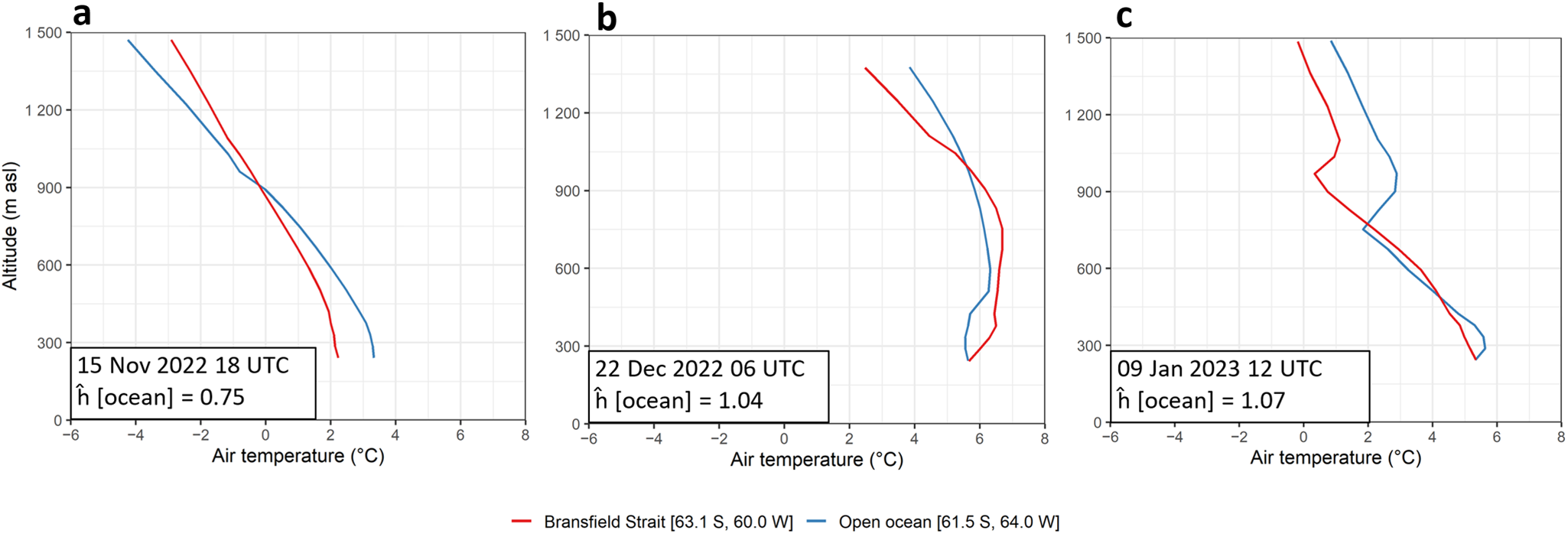
Figure 10. WRF-based vertical profiles of air temperature windward of northern James Ross Island on 15 November 2022 18:00 UTC (a), 22 December 2022 06:00 UTC (b), 09 January 2023 12:00 UTC (c). Two points are shown: open Southern Ocean (61.5°S, 64.0°W) and the Bransfield Strait (63.1°S, 60.0°W). Also the non-dimensional mountain height (ĥ) computed over all model layers with altitude >200 m and <1500 m is shown.

3.3.3. Vertical displacement and thermodynamical properties of foehn trajectories

The backward trajectories for the peak phases of the three investigated events revealed that the source region of foehn flow varied slightly across the events (Fig. 11). In the peak phase of the Nov 22 event, which was generally less intense and had smaller vertical velocities (Fig. S6), the mean altitude of the foehn flow before reaching the AP was 1030 m a.s.l. (Table 3). In the more intense Dec 22 and Jan 23 events, the mean altitude of backward trajectories in the source region was 1143 m a.s.l. and 1331 m a.s.l., respectively. In addition, during the first event, an updraft of foehn flow before reaching and overcoming the AP mountains was more developed than during the subsequent events when the incoming flow was characterised by less inclined trajectories before undergoing rapid descent eastward of the AP mountain ridge. During the cross-AP transition, the foehn flow warmed by 5.2°C (Nov 22), 7.0°C (Dec 22) and 9.5°C (Jan 23) while the potential temperature decrease was 1.6 K (Nov 22), 1.1 K (Dec 22) and 0.0 K (Jan 23) (Table 3).

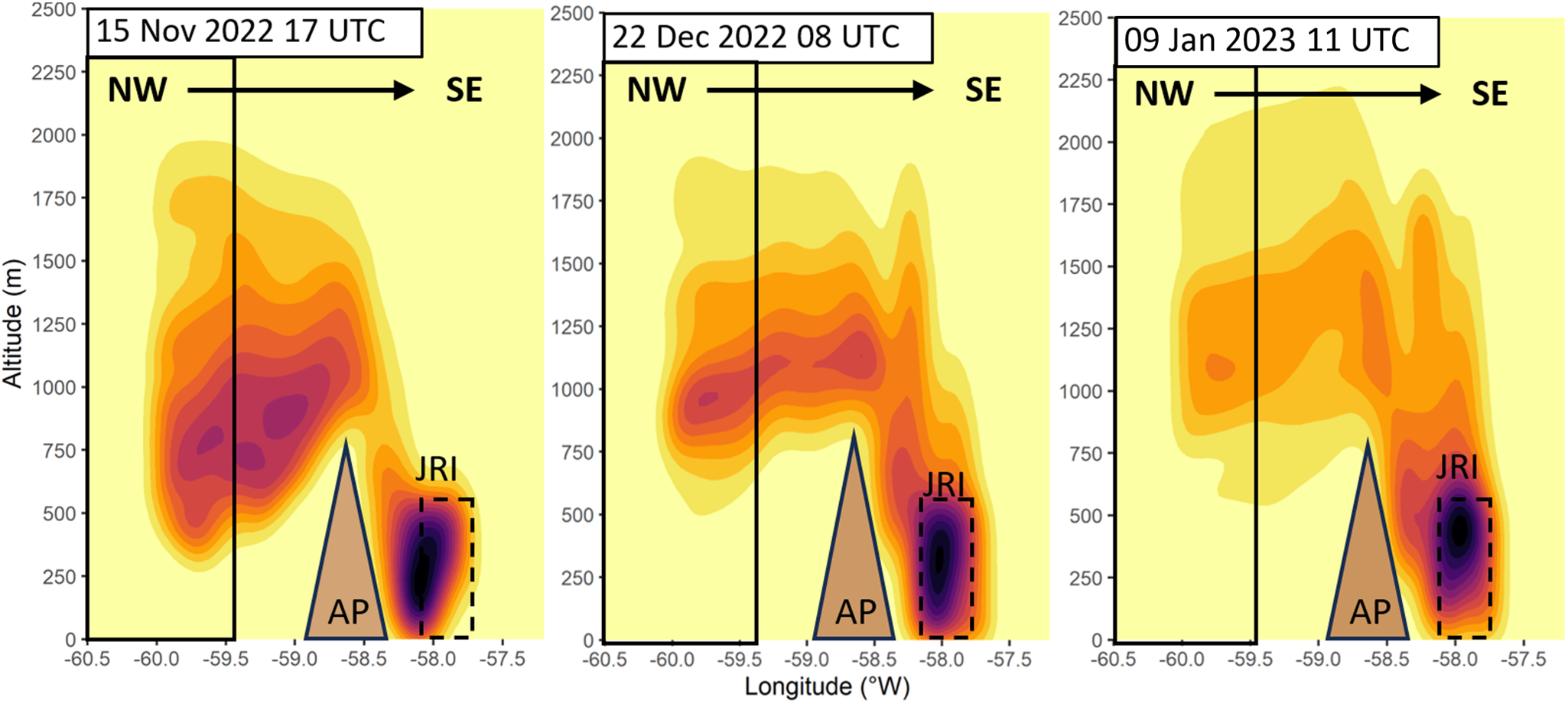
Figure 11. Kernel density of backward trajectories originating westward of the Antarctic Peninsula and reaching the northern James Ross Island during the peak phase of ablation events. The solid rectangle marks the source region of foehn flow, the dashed rectangle the target region over the northern JRI and brown triangles show the Antarctic Peninsula. The mean air temperature, potential air temperature, equivalent potential air temperature, mixing ratio and altitude characteristics of the source and target regions are provided in Table 3.

Table 3. The mean altitude, air temperature, potential air temperature ( $\theta$), equivalent potential air temperature ( $\theta$e), difference between mean equivalent potential air temperature and mean potential air temperature ( $\theta$e − $\theta$) and the mixing ratio (g kg^-1) of the source region of foehn flow (i.e. west of 59.4°W and north of 63.75°S) and the target region over northern JRI (i.e. 63.7732°S–63.8922°S; 57.7254°W–58.1362°W) during the peak phases of the selected ablation events Nov 22, Dec 22, and Jan 23

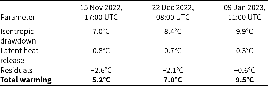
To evaluate the role of latent heat release, equivalent potential temperature and the mixing ratio of foehn flow before and after crossing the AP were quantified. The difference between equivalent potential temperature and potential temperature (θe − θ) mirrors the moisture content and any change in this difference can be attributed to latent heat release (or consumption). The (θe − θ) difference changed by 0.8 K (Nov 22), 0.7 K (Dec 22) and by 0.3 K (Jan 23) during the air transport from the source to the target region (Table 3). It corresponds to a moderate decrease in water vapour mixing ratio by 0.27 g kg⁻¹ (Nov 22), 0.20 g kg⁻¹ (Dec 22) and by 0.14 g kg⁻¹ (Jan 23). The impact of isentropic drawdown (computed following Cape and others, 2015 and using the dry adiabatic lapse rate), latent heat release (obtained from [θe − θ]) and residuals (i.e. the radiative and turbulent heat fluxes) on total foehn warming is highlighted in Table 4.

Table 4. Summary of the impact of isentropic drawdown, latent heat release and residuals on total foehn warming during the investigated events

3.4. Regional context of surface heat fluxes and snow and ice melting during intense ablation events

For the highest ablation day on the Triangular Glacier in each studied event, the daily means of surface energy fluxes were computed for the glaciers in the WRF domain D04 (Fig. 12), focused on the northern JRI and adjacent slopes of other islands and the AP. The sensible heat flux reached its maximum over the southeastern AP slopes and lower-elevated glaciers on the northwestern part of the Ulu Peninsula. This could be related to very high air temperature observed in these areas (Figs. 7, S6, S8) The mean daily fluxes in these areas reached mostly 50–100 W m⁻² on 22 November 2022. At the peak day of the Dec 22 event, the mean sensible heat flux often exceeded 200 W m⁻² and, locally, even 300 W m⁻². Very high values were also simulated on 09 January 2023, when the Jan 23 event peaked.

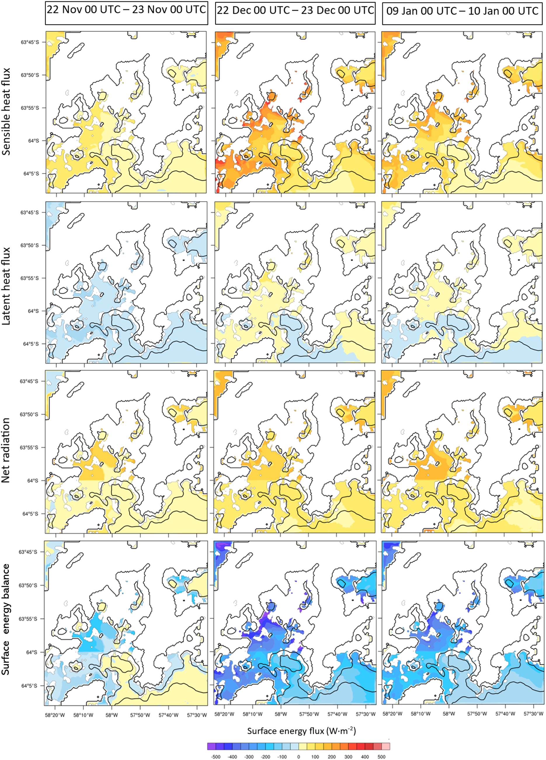
Figure 12. Mean daily sensible and latent heat fluxes, net radiation and surface energy balance (leading to warming or melt) on northern JRI glaciers. The values for the day with the highest ablation within each event in summer 2022/2023 are shown. WRF model outputs, domain D04 (300-m horizontal resolution). Ice-free areas and ocean are masked. The contours (black lines) are given at 400-m interval.

The latent heat flux was mostly negative on 22 November 2022, ranging from −50 W m⁻² to 0 W m⁻². During the peak phase of the Dec 22 and Jan 23 events, the latent heat flux turned to positive values at numerous glaciers, mainly with an altitude below 500 m a.s.l. Net radiation was also a significant energy source for northern JRI glaciers, with the mean values reaching mostly 100–200 W m⁻² on the low-elevated glaciers, while at higher locations, the flux ranged within 0–100 W m⁻². Note that the isolines following 64°S and 320 m a.s.l. are related to the WRF model initial snow conditions (see Section 2.4).

The SEB on the peak days affected the resulting energy flux into the snow cover or glacier ice. On 22 November 2022, the glaciers on the northwestern JRI below 400 m a.s.l. were subject to energy input of 100–250 W m⁻² while the areas above ∼500 m a.s.l. experienced a slight energy loss. The peak day of the Dec 22 event led to a mean energy input of 300–500 W m⁻² over extensive areas and, locally, even >500 W m⁻² over the lowest sections of Ulu Peninsula glaciers. The last event was slightly less intense on its peak day; however, local maximum values of 400–500 W m⁻² also appeared in the study area.

To evaluate the regional relevance of ablation intensity on northern JRI, the WRF D03-based cumulative surface melt for each ablation period was plotted (Fig. 13). During the Nov 22 event, intense melt occurred only on JRI, eastern AP slopes and smaller islands east of AP. The warmer Dec 22 and Jan 23 events also induced slight melt around the western AP coast; however, the eastern AP as well as JRI and Vega Island, experienced very intense melt. Extensive surface melt over the northern AP region was also confirmed by satellite images obtained with the MODIS/Aqua Snow Cover Daily L3 Global 500 m SIN Grid product (Fig. S9).

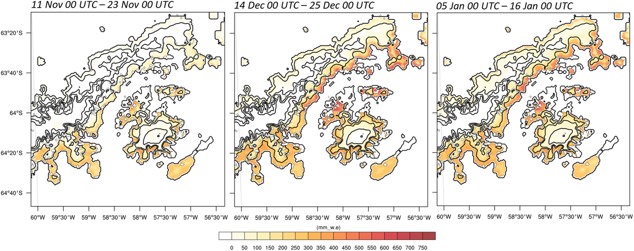
Figure 13. Cumulative surface melt simulated by the WRF model on James Ross Island and Antarctic Peninsula glaciers during the selected extreme ablation events in the summer of 2022/23. The contours (black lines) are given at 400-m interval.

4. Discussion

4.1. The WRF model performance

The WRF model in very high horizontal resolution successfully captured air temperature and wind speed measured on Triangular Glacier and Davies Dome and net radiation on Triangular Glacier (Figs. 4, S1, S3). Despite generally good model performance, we acknowledge that the simulated wind speed manifested a slight positive bias. The exact source of the bias is not clear and would require a deeper investigation, which is outside the scope of this study. Using a numerical model with a horizontal resolution of 300 m made it possible to quantify the energy fluxes even over small glaciers, which are found on northern JRI. We suggest that further increasing model resolution could possibly improve performance in small-scale topography areas, such as the Triangular Glacier located in a relatively small cirque partly surrounded by steep cliffs. At Mendel station, located on the northern coast of JRI, a noticeable reduction in wind speed bias was obtained when the WRF model resolution was increased from 700 to 300 m (Matějka and Láska, 2022). In contrast, no clear or significant improvement was found for enhanced model resolution over the LIS either for Polar WRF (Turton and others, 2017) or the MetOffice Unified Model (Orr and others, 2021). Our results suggest that the benefits of increased model resolution are significantly higher in areas with rough topography and land-cover mosaic than on more uniform ice shelves. However, rather long simulation periods and the rapidly growing computational costs with model resolution (e.g. Warner, 2010) prevented us from assessing this further.

Furthermore, the choice of land-surface model computing snow cover evolution (NoahMP in this study) within the WRF framework and the initial snow height and density may have some influence on model accuracy. Unfortunately, in this region, no high-resolution snow height products are available, and pointwise observations are very scarce. In addition, snow mass on the JRI glaciers is massively redistributed by wind (Engel and others, 2024), making an accurate definition of snow initial conditions even more challenging. The influence of initial conditions can be reduced during the model spin-up time (≥6 days in this study), but the initialisation-related patterns can persist even longer and should be considered when interpreting model results (e.g. Fig. 12). The sensitivity of modelled snow cover to forcing data can be assessed using an extensive ensemble of model realisations (Voordendag and others, 2021). However, this approach would be extremely computationally intensive for the very high-resolution model setup selected, but it might provide a topic for future research.

4.2. Surface energy fluxes and their spatial variability

During all melt events, net radiation was the most important source of heat for snow and ice melting on Triangular Glacier (observations: 81–129 W m⁻², WRF outputs: 90–149 W m⁻²). Sensible heat flux simulated by the WRF model reached slightly lower but still significant values of 70–99 W m⁻², while latent heat flux was mostly negative (i.e. sublimation and evaporation outweighted deposition and condensation), reaching −46 to −23 W m⁻². Davies Dome experienced significantly lower values of both net radiation and sensible heat flux and more negative latent heat flux, together dramatically reducing available energy used for snow warming or melting by 100–152 W m⁻², that is, by 69%–87%. This contrast suggests the importance of local factors (e.g. altitude, slope, aspect, snow or ice properties) involved in atmosphere–cryosphere interactions within complex areas, such as the northern JRI, and the necessity and benefits of using a numerical model in hundreds-of-metres horizontal resolution. We are aware that the simulated fluxes are subject to uncertainty. Generally, the WRF model slightly underestimated air temperature and overestimated wind speed, and both errors can affect sensible heat flux estimates. For comparison, the peak simulated values (400–500 W m⁻²) are moderately higher than the peak values of around 300 W m⁻² presented over the LIS (Wiesenekker and others, 2018; Elvidge and others, 2020; Gorodetskaya and others, 2023).

4.3. Foehn wind mechanism

The results suggest that foehn wind played an important role during the peak phases of all extreme ablation events. The Nov 22 event was rather weak, with the highest air temperatures confined mostly to narrow leeward regions of AP and JRI (Fig. S6). In contrast, the Dec 22 and Jan 23 events were both marked by a strong, widespread foehn flow extending tens of kilometres over the JRI region into the Weddell Sea as can be seen in Figs. 7 and S8. Following the analyses in Section 3.3, we suggest that the leading foehn mechanism of all events was isentropic drawdown. Latent heat release due to precipitation contributed to the total warming by <1 K. A relatively higher contribution of 0.7–0.8 K was identified during the Nov 22 and Dec 22 events while lower contribution of 0.3 K was found during the Jan 23 event. This might be related to generally lower precipitation over the Bransfield Strait N/NW from the investigated JRI glaciers (Fig. 9). The relatively larger role of latent heat during the Nov 22 event is also related to (1) the smaller altitudinal difference between the foehn wind source region and the affected leeward region and (2) the lower source altitude of the foehn air mass. A partial tendency to linear flow-over regime during this event was also reflected by the lowest ĥ value among investigated events. Meanwhile, the Dec 22 and Nov 23 events featured a substantial blocking of low-level flow and downdraft of air with higher potential temperatures from above the blocked layer. Interestingly, blocking occurred under relatively low values of non-dimensional mountain height ĥ, reaching only slighty above 1. We suggest, in agreement with Elvidge and others (2015), that an elevated inversion (Jan 23) or a deep isothermal layer (Dec 22) played an important role for the blocking regime establishment. In contrast to the investigated events, in Case C of Elvidge and Renfrew (2016a, 2016b), the source region was only around 300 m above sea level, and foehn warming was primarily attributed to latent heat release and precipitation occurrence. Similar to that Case C, the foehn leading to the all-time Antarctic record of 18.3°C at Esperanza station (06 February 2020) had the initial altitude of foehn flow at only ∼120 m a.s.l. (Xu and others, 2021). Meanwhile, the isentropic drawdown played an important role in extreme atmospheric warming at the Marambio station recorded on 09 February 2020 (Bae and others, 2022). This suggests that the intense foehn-related AP heat waves can be forced dominantly by both isentropic drawdown and latent heat release. Whether the importance of individual mechanisms varies locally within the region or whether their role is changing during the current climate change is unclear and should be emphasised in future investigations. Finally, our results advocate that isentropic drawdown-related foehn can cause extensive warming and induce large-scale snow and ice melt over the JRI region.

4.4. Regional context of intense snow and ice melting in the summer season of 2022/23

Three investigated extreme ablation events on JRI led to a total surface ablation of 271 mm w.e. on Davies Dome and 1237 mm w.e. on Triangular Glacier and significantly contributed to an exceptional glacier mass loss in the glaciological year 2022/23 on JRI. We suggest that the rapid melting of winter snow cover during the first event (see Supplementary Material for more details) was supportive to significant ice melt during the subsequent events and very high cumulative ablation, especially on low-elevated glaciers. Finally, we can infer that chained foehn events, as observed during summer 2022/23, can significantly impact seasonal and annual glacier mass balance in the eastern AP sector. Similar future events can have an even bigger impact on the cryosphere, as the AP heat waves are already intensifying due to ongoing climate change (González-Herrero and others, 2022). Furthermore, the frequency and intensity of extreme heat waves can increase during future positive-SAM-index phases as the index values and the northeastern AP air temperatures were found to be significantly correlated (Clem and others, 2016). The increase in SAM has already accelerated the late 20th-century warming in the region (Orr and others, 2008).

Due to the exceptional impact of these heat waves on atmospheric boundary layer processes, the cryosphere and surface runoff in ice-free areas (Syvitski and others, 2022), there is an urgent need for the analysis of their drivers and consequences, not only in the AP region but elsewhere in Antarctica. For example, Wille and others (2024a, 2024b) investigated the impacts of an intense atmospheric river transporting large amounts of heat and moisture to the Antarctic interior, resulting in a record-breaking heat wave and massive snow accumulation over a large section of the Eastern Antarctic Ice Sheet, and contributing to the final collapse of the Conger Ice Shelf (Lhermitte and others, 2023). Furthermore, warm air intrusions related to atmospheric rivers were shown to induce multi-day surface melt over Pine Island Glacier, West Antarctica (Djoumna and Holland, 2021). It was shown that foehn winds have a notable impact on the Pine Island Glacier using ERA5 reanalysis data (Francis and others, 2023). While the ERA5 could provide data of very high quality, we suggest that the use of a very high-resolution model (e.g. WRF, MetUM) could further improve the understanding of foehn dynamics and impacts also in this sensitive region.

It is noteworthy that massive glacier ice melt during the 2022/23 summer was not restricted to JRI only. Based on the WRF model output, we detected extensive snow and glacier ice melt on northeastern AP glaciers in elevations below ∼400 m a.s.l. (Nov 22) and ∼600 m a.s.l. (Dec 22 and Jan 23). Vega Island and Snow Hill Island were also significantly affected. In the glaciological year of 2022/23, the Glaciar Bahía del Diablo on Vega Island experienced the most negative mass balance since the beginning of observations in 1999/2000 (World Glacier Monitoring Service, 2023, 2024). Our findings suggest that the investigated events indeed contributed to the extremely negative mass balance on Vega Island. However, a detailed analysis has not yet been performed. In contrast, only slight-to-moderate melt was found on the western AP slopes, which could be related to air temperature lower by ∼4–8°C during foehn events compared to the eastern AP region (Figs. 7, S6, S8). Meanwhile, during the February 2022 event, the extreme melt was more symmetrical around the AP mountain ridge due to exceptionally high air temperatures on the western AP related to the rapid advection of very warm and moist air from the north (Gorodetskaya and others, 2023). The summer 2022/23 events were driven by slightly cooler northwestern advection, and as a result, very high air temperatures were limited to the foehn-affected eastern AP region. Finally, this study suggests that foehn winds can massively accelerate snow and ice melt not only in the LIS region (Kuipers Munneke and others, 2018; Elvidge and others, 2020) but also in both the JRI region and adjacent AP slopes.

The potential record-breaking melt duration observed in the northern AP region during the summer of 2022/23 could be further investigated using remote sensing data such as microwave backscatter imagery (e.g. Barrand and others, 2013) or Sentinel-1 data (Liang and others, 2021), which offer a more detailed picture of surface melt extent and timing with spatial resolutions of up to 40 m. Furthermore, any future research dealing with atmosphere–cryosphere interactions could benefit from a complex snow model deployed within the WRF modelling framework. An example is the WRF-ice (Luo and others, 2021) or the recently released CRYOWRF (Sharma and others, 2023). The latter is indeed currently adapted for snow-climate applications in the AP region, where it could significantly improve the simulation of blowing snow events, which significantly affect the spatial patterns of glacier mass balance (Engel and others, 2018).

5. Conclusions

Three major melt events associated with foehn winds in the northern AP region in the summer of 2022/23 were investigated using in-situ observations and WRF model simulations. Emphasis was given to synoptic-scale and local atmospheric processes, the foehn mechanism and its impact on rapid snow and ice melt, aiming to improve our understanding of physical basis and impacts of highly relevant Antarctic heat waves. The WRF model in very high resolution proved to be extremely valuable for this investigation. The model captured near-surface atmospheric conditions well, slightly underestimating air temperature by around 1°C and slightly overestimating wind speed by 1–2 m s⁻¹. However, further improvement is needed in simulating snow-related processes, such as wind-driven snow transport. To overcome this limitation, we suggest the deployment of the newly released CRYOWRF model, which explicitly simulates these processes and potentially improves the estimation of glacier mass balance.

The investigated events led to a total surface ablation of 271 mm w.e. on Davies Dome and 1237 mm w.e. on Triangular Glacier, contributing substantially to the unusually negative mass balance of the JRI glaciers in the 2022/23 glaciological year. Particularly, the surface mass loss on Triangular Glacier was ≥4 times higher than 2014/15–2019/20 average, while also Davies Dome experienced a notable mass loss of 270 mm w.e., compared to the slightly positive 2009/10–2020/21 mean. The WRF model output indicates extensive snow and glacier ice melt also on the northeastern AP glaciers and smaller islands of the JRI archipelago, such as Snow Hill and Vega Island. Simulated melt on the western AP coast was significantly less intense, corresponding with lower air temperatures during foehn events. The first event in November 2022, while the least intense, resulted in the complete loss of the winter snow cover on Triangular Glacier. The bare ice subsequently melted rapidly in the following melt season. During very warm conditions on Triangular Glacier in December 2022 and January 2023 (with temperatures up to 10–12°C), ice melt rates of 50–100 mm w.e. per day were observed repeatedly. Davies Dome experienced less intense surface lowering, with only 2 days of daily melt exceeding 20 mm w.e. Altogether, our results indicate that consecutive foehn events can significantly contribute to seasonal glacier mass loss and negative annual mass balance in the northeastern AP region. For example, on Triangular Glacier, the three studied events were responsible for ∼77% of surface ablation between 01 February 2022 and 16 January 2023, while on Davies Dome, they led to ablation almost equal to annual mass loss.

During the studied events, the net radiation and sensible heat flux were the principal contributors to snow and glacier ice warming and melt, similar to a foehn event on the LIS in November 2010 (Kuipers-Munneke and others, 2012). Triangular Glacier received significantly higher fluxes compared to Davies Dome, increasing the available energy for glacier surface warming or melting by 100–152 W m⁻². This contrast can be related to higher air temperature and notably higher net radiation values on the Triangular Glacier (Table 2). This highlights the substantial local variations in energy and mass fluxes at the glacier–atmosphere interface, underlining the need for high-resolution models to capture these interactions in the complex topography of the AP region. Considering the regional context, our estimates show that the highest glacier surface energy input (combining net radiation, sensible and latent heat fluxes) occurred on glaciers on JRI, Vega Island and the northeastern AP slopes in elevations below 400 m a.s.l. During the widespread foehn event on 22 December 2022, the mean daily values of this combined energy flux locally exceeded 400 W m⁻². Only slightly lower values were estimated during the culmination of the following event on 09 January 2023.

Foehn flow over the AP mountains and associated leeside warming significantly contributed to the peak phases of the three melting episodes. The backward-trajectory analysis revealed that the primary foehn mechanism was an isentropic drawdown. The flow was adiabatically heated when descending by ∼700–1000 m. The isentropic drawdown was further supported by latent heat release, which contributed by 0.3–0.8 K to total foehn warming, most significantly in the Nov 22 event. This event also featured the lowest source altitude of foehn wind and lowest descent of foehn trajectories. The Dec 22 and Jan 23 events were accompanied by low-level blocking of incoming flow due to the presence of temperature inversion or a an isothermal layer. This led to the dominant role of isentropic drawdown in foehn warming during these events.

The presented results show that chained summer foehn events could induce anomalously intense melt in the eastern AP region (e.g. they largely contributed to ≥4 times higher-than-average annual surface mass loss on Triangular Glacier). This study also stresses the importance of further investigations on Antarctic heat waves, which are becoming more intense due to ongoing climate change and could significantly affect multiple components of the sensitive Antarctic geosystems.

Finally, the most important results can be summarised as follows:

• • Three intense chained foehn events during the summer of 2022/23 led to anomalously large glacier surface ablation in the northeastern AP region.

• • In a very high resolution of 300 m, the WRF model allowed for the investigation of foehn’s impact in a great detail, which is of utmost importance in the complex topography of northern AP and other Antarctic regions. Some challenges, however, remain in modelling the intricate atmosphere–cryosphere interactions. A prime example is an accurate setup of a snow model and initial conditions of snow cover.

• • The leading foehn warming mechanism was isentropic drawdown with small and variable contributions from latent heat release.