


1. Introduction
The initiation and propagation of macroscale fractures (also known as rifts) on ice shelves acts as a significant control on the rate of mass loss from the Antarctic Ice Sheet. The propagation of active rifts both vertically and laterally can result in the calving of tabular icebergs, which directly contributes ice mass to the oceans (Evans and others, Reference Evans, Fraser, Cook, Coleman and Joughin2022). Further, even fractures that do not directly result in calving events can weaken the backstress that ice shelves provide to grounded ice, an effect known as buttressing. The loss of load-bearing, and thus buttressing ability, of ice shelves can result in accelerated mass flow to the ocean from the grounded ice, further adding to mass loss and affecting the stability of large regions of the ice sheet (Borstad and others, Reference Borstad, E, J and MP2013, Reference Borstad, Khazendar, Scheuchl, Morlighem, Larour and Rignot2016, Reference Borstad, McGrath and Pope2017; Sun and others, Reference Sun, Cornford, Moore, Gladstone and Zhao2017; Reese and others, Reference Reese, Gudmundsson, Levermann and Winkelmann2018; Lhermitte and others, Reference Lhermitte2020; Mitcham and others, Reference Mitcham, Gudmundsson and Bamber2021; Sun and Gudmundsson, Reference Sun and Gudmundsson2023; Surawy-Stepney and others, Reference Surawy-Stepney, Hogg, Cornford and Davison2023).
Additionally, the development and propagation of fractures can result, in certain cases, in the collapse of large regions of ice shelves, as occurred in the case of the Larsen B Ice Shelf (Doake and others, Reference Doake, Corr, Rott, Skvarca and Young1998; Banwell and others, Reference Banwell, MacAyeal and Sergienko2013). Rapid breakup of ice is also occurring on Thwaites Ice Shelf in possibly a similar process (Lhermitte and others, Reference Lhermitte2020; Benn and others, Reference Benn2022; Surawy-Stepney and others, Reference Surawy-Stepney, Hogg, Cornford and Davison2023), and other regions of Antarctic ice shelves may be vulnerable to similar instabilities (Lai and others, Reference Lai2020). These collapses remove the buttressing effect and likely result in acceleration of grounded ice toward the ocean (Fürst and others, Reference Fürst2016), as has been identified after the Larsen B breakup (Rignot, Reference Rignot, Casassa, Gogineni, Krabill, Rivera and Thomas2004; Scambos, Reference Scambos, Bohlander, Shuman and Skvarca2004). Further, they may have large-reaching consequences for the stability of the Antarctic Ice Sheet, though the extent of these consequences remains unknown (Pollard and others, Reference Pollard, DeConto and Alley2015; DeConto and Pollard, Reference DeConto and Pollard2016; Clerc and others, Reference Clerc, Minchew and Behn2019; Edwards and others, Reference Edwards2019; Robel and Banwell, Reference Robel and Banwell2019; Bassis and others, Reference Bassis, Berg, Crawford and Benn2021; Crawford and others, Reference Crawford, Benn, Todd, Astrom, Bassis and Zwinger2021; Golledge and Lowry, Reference Golledge and Lowry2021; Schlemm and others, Reference Schlemm, Feldmann, Winkelmann and Levermann2022).
An important step toward reducing uncertainty in sea level rise projections is understanding how fracturing affects the flow of upstream ice and implementing this dynamic in models. The current lack of observations on large-scale ice shelf failure and limited observations on calving events, in addition to uncertainties in ice rheology and the grain-scale processes through which failure occurs, impede the predictive capability of models. A strong foundation for understanding material failure already exists. Fracture criteria, also known as yield criteria or failure envelopes (a relationship between the strength of a material and the stresses applied to it), are well-studied in material science, several engineering disciplines, and within the glaciological literature. Many different criteria have been applied to describe the nature of ice fracture and to model iceberg calving (Pralong and Funk, Reference Pralong and Funk2005; Albrecht and Levermann, Reference Albrecht and Levermann2012; Duddu and Waisman, Reference Duddu and Waisman2012), as well as materials sometimes used as mechanical analogs for ice (e.g. Drucker and Prager, Reference Drucker and Prager1952; Bhat and others, Reference Bhat, Choi, Wierzbicki and Karr1991). Other approaches have included using a pressure threshold (Duddu and others, Reference Duddu, Jiménez and Bassis2020) and a strain threshold (Duddu and Waisman, Reference Duddu and Waisman2012), though these are currently less used in large-scale ice sheet models. Most numerical models that represent ice fracture and calving use a stress threshold, which describes a critical stress above which ice fractures (Hulbe and others, Reference Hulbe, LeDoux and Cruikshank2010; Borstad and others, Reference Borstad, Khazendar, Scheuchl, Morlighem, Larour and Rignot2016; Jiménez and others, Reference Jiménez, Duddu and Bassis2017; Lai and others, Reference Lai2020). While many of these studies benchmark their models against laboratory estimates, few studies have been able to use observations of natural systems to determine the proper fracture criterion and stress threshold for ice fracture.
Even within models that use a stress threshold, the magnitude of the critical stress or the relationship of the critical stress to principal stresses is not generally agreed upon. Various models use critical stresses, also known as the strength of ice, ranging from 0.1 to 1 MPa, an order of magnitude difference (Pralong and others, Reference Pralong, Funk and Lüthi2003; Pralong and Funk, Reference Pralong and Funk2005; Astrom and others, Reference Astrom2013; Reference Astrom2014; Duddu and Waisman, Reference Duddu and Waisman2013; Krug and others, Reference Krug, Weiss, Gagliardini and Durand2014; Benn and others, Reference Benn2017). These thresholds are based on laboratory experiments and glaciological observations. Laboratory experiments provide a range of values from 500 kPa to as high as 5 MPa (Currier and Schulson, Reference Currier and Schulson1982; Lee and Schulson, Reference Lee and Schulson1988; Druez and others, Reference Druez, McComber and Tremblay1989; Petrovic, Reference Petrovic2003), while observations have found a lower range of tensile strengths from 76 kPa to 1 MPa (Vaughan, Reference Vaughan1993; Ultee and others, Reference Ultee, Meyer and Minchew2020; Chudley and others, Reference Chudley2021; Grinsted and others, Reference Grinsted, Rathmann, Mottram, Solgaard, Mathiesen and Hvidberg2024). Ultee and others Reference Ultee, Meyer and Minchew(2020) found the tensile strength of ice to be  $\sim 1$ MPa by considering relatively undeformed and intact ice on Vatnajokull Ice Cap in Iceland and determining the highest stresses present in unfractured ice using linear-elastic mechanics (no assumed n value). While this provides a useful baseline for ice strength in relatively undeformed and undamaged ice, the exact applicability to the conditions on Antarctic ice shelves, where ice has a longer history of deformation, and thus more accumulated damage or impurities, remains unclear. Vaughan Reference Vaughan(1993), using stresses calculated from observed strain rates (and assuming n = 3), found the tensile strength of ice in regions of Antarctica ranged from 90 to 320 kPa, below the lower bound of strengths estimated by laboratory experiments. However, due to limited observations available in the early 1990s, the broader applicability of Vaughan’s results to the entire Antarctic Ice Sheet is unclear. Grinsted and others (Reference Grinsted, Rathmann, Mottram, Solgaard, Mathiesen and Hvidberg2024) finds tensile strengths of $\sim 150$–250 kPa, and Chudley and others (Reference Chudley2021) find an even lower critical stress of 76 kPa for fractures on the Greenland Ice Sheet, again assuming n = 3. The difficulty of measuring stresses in situ necessitates an assumption of ice rheology to calculate the critical stress threshold, which introduces inconsistencies between observations and laboratory-derived stress measurements. It is vital to understand the differences that assumptions in ice rheology make in estimates of tensile strength, as variables such as deformation mechanism, flow speed, and other material properties of the ice that vary regionally can affect rheology and therefore strength (Mellor, Reference Mellor1979; Currier and Schulson, Reference Currier and Schulson1982; Ranganathan and others, Reference Ranganathan, Minchew, Meyer and Peč2021b; Ranganathan and Minchew, Reference Ranganathan and Minchew2024). This knowledge gap makes a complete study of the stress threshold across the Antarctic Ice Sheet, capturing many different flow regimes, necessary and motivates this study.
Here, we use high-resolution, remotely sensed observations of surface strain-rate fields (Gardner and others, Reference Gardner2018) and optical imagery of ice fractures (Haran and others, Reference Haran, Bohlander, Scambos, Painter and Fahnestock2014, Reference Haran, Klinger, Bohlander, Fahnestock, Painter and Scambos2019, Reference Haran, Bohlander, Scambos, Painter and Fahnestock2021) to estimate surface stresses around areas of large-scale rifting. We use these stresses to evaluate and calibrate fracture criteria that may be used in ice sheet models to represent rifting and calving. We consider five such criteria in this study—Mohr–Coulomb, von Mises, strain energy, Drucker–Prager, and Hayhurst—each of which we describe in some detail. Due to more recent and abundant satellite data, we can capture and evaluate numerous fractures across Antarctic ice shelves, enabling a more complete look at fracturing in different regions of the Antarctic Ice Sheet.
2. Methods
2.1. Identifying fractures
We manually identify fractures on Amery (AIS), Larsen C (LCIS), Ronne–Filchner (RFIS), and Ross (RIS) Ice Shelves as these ice shelves are large, contain easily identifiable large-scale fractures and fractures isolated from larger fracture fields or other areas with accumulated damage that could influence ice rheology, and, in particular to the AIS and LCIS, have fractures that contribute to iceberg calving events after 2014. We do not initially investigate more rapidly changing areas of Antarctica such as the ice shelves in the Amundsen Sea Embayment, as the dynamic nature of these ice shelves introduces many uncertainties into rheological processes. We will examine the ice shelves of the Amundsen Sea Embayment later on to test the applicability of our derived framework on more complex areas of Antarctica.
We identify fractures using 2014–2015 Landsat-8 derived 240 m × 240 m effective strain rate fields (Gardner and others, Reference Gardner2018) and MODIS Mosaic of Antarctica (MOA) 2014 optical imagery (Scambos and others, Reference Scambos, Haran, Fahnestock, Painter and Bohlander2007; Haran and others, Reference Haran, Bohlander, Scambos, Painter and Fahnestock2014). We look for linear features with high strain rates in the strain-rate data, and linear, fracture-like features in MOA imagery on each ice shelf, and trace the identified features in QGIS. From these traces, we create two datasets: one of crevasse features that can be identified on both optical imagery and strain rate fields, and one of crevasse features that can be identified only on optical imagery. We refer to the first category as ‘active crevasses’ and the latter ‘inactive crevasses’. The purpose of searching for high-strain-rate crevasses is to filter out crevasses that may have advected downstream to a stress state different from the conditions under which they formed. We aim to include active crevasses rather than inactive crevasses to gain a better understanding of the stresses associated with fracture propagation and note that inactive crevasses may exist at stress states similar to those of unfractured ice. We avoid including crevasses that exist close to large chains of crevasses or other features indicative of ice damage, as damage can introduce uncertainties into rheological parameters such as the flow rate parameter A. In optical imagery, it is difficult to distinguish the depth of crevasses, and as such, both surface crevasses and full-thickness rifts are likely included in our datasets, and in either case, the high strain rates across the crevasse indicate widening. We find a total of 36 active crevasses out of a total of 110 crevasses identified on optical imagery (Fig. 1). Of the 36 active crevasses, we find 4 on AIS, 9 on LCIS, 9 on RFIS and 14 on RIS. We sample principal deviatoric stresses at each pixel overlapped by a fracture trace on our calculated stress fields.

Figure 1. Fractures observed via optical imagery (dark green) and strain rate (neon green) data over the four ice shelves of interest: (a) Ronne–Filchner (RFIS), (b) Amery (AIS), (c) Larsen C (LCIS) and (d) Ross (RIS). Ice upstream of the grounding line is masked in gray (Morlighem, Reference Morlighem2019) and not considered in estimates of ice strength. (e) An example of identified crevasses on the RIS as seen on MOA2014 (left) and strain rate fields (right). (f) An example of active crevasses on the RIS as seen on MOA2014 (left) and strain rate fields (right). The inset in (a)–(d) shows ice velocity over Antarctica (Rignot and others, Reference Rignot, Mouginot and Scheuchl2017), with the aforementioned ice shelves boxed in red. We do not mask grounded ice in the inset.
To compare the difference in stress states present in crevassed ice and uncrevassed ice, we sample principal deviatoric stresses of unfractured ice upstream of areas of crevasse fields and in unfractured areas near the calving front. We avoid sampling stresses in suture zones, as previous studies have shown crevasse propagation is slowed or stopped by suture zones, suggesting the ice present in such areas has a higher tensile strength (Glasser and others, Reference Glasser2009; Holland and others, Reference Holland, Corr, Vaughan, Jenkins and Skvarca2009; Hulbe and others, Reference Hulbe, LeDoux and Cruikshank2010; Borstad and others, Reference Borstad, McGrath and Pope2017). By comparing the stresses present in relatively undamaged and actively crevassed ice, as close to the crevasses as the data allow, we can delineate a stress threshold, or failure envelope, at which ice will fail. The spatial resolution of the data are too coarse to allow for constraints on the intensification of stresses near fracture tips.
2.2. Stress calculations
To study the conditions under which ice fractures, we calculate deviatoric stresses on ice shelves from observed horizontal strain rate fields and the assumptions of incompressible ice and negligible vertical shear. We calculate the strain rate tensor at each map location from the gradient of the Landsat-8 derived surface velocity fields (Gardner and others, Reference Gardner2018). We calculate the gradient using a 2nd-order Savitsky–Golay filter and a 2 km window, as in Minchew and others Reference Minchew, Simons, Riel and Milillo(2017). The principal strain rates are the eigenvalues of the strain rate tensor. We calculate the effective strain rates (the square root of the second invariant (I 2) of the 3-D strain-rate tensor) from principal strain rates as
 \begin{align}
\dot{\epsilon}_E = \sqrt{{I}_2(\dot{\epsilon}_{ij})} = \sqrt{\dot{\epsilon}_{1}^2 + \dot{\epsilon}_{2}^2 + \dot{\epsilon}_{3}^2}
\end{align}
\begin{align}
\dot{\epsilon}_E = \sqrt{{I}_2(\dot{\epsilon}_{ij})} = \sqrt{\dot{\epsilon}_{1}^2 + \dot{\epsilon}_{2}^2 + \dot{\epsilon}_{3}^2}
\end{align} where  $\dot{\epsilon}_1$ is the most tensile horizontal principal strain rate and $\dot{\epsilon}_2$ is the least tensile horizontal principal strain rate. We adopt the sign convention of positive tensile values ( $\dot{\epsilon}_1 \ge \dot{\epsilon}_2$). We take ice to be incompressible (i.e. $0 = \dot{\epsilon}_{1} + \dot{\epsilon}_{2} + \dot{\epsilon}_{3}$). We then solve for $\dot{\epsilon}_{3}$ and substitute into Eqn 1, solving for effective strain rate in terms of only the horizontal principal strain rates:
 \begin{align}
\dot{\epsilon}_E = \sqrt{\dot{\epsilon}_1^2 + \dot{\epsilon}_2^2 + \dot{\epsilon}_1\dot{\epsilon}_2}.
\end{align}
\begin{align}
\dot{\epsilon}_E = \sqrt{\dot{\epsilon}_1^2 + \dot{\epsilon}_2^2 + \dot{\epsilon}_1\dot{\epsilon}_2}.
\end{align}Because shear stresses at the upper and lower surfaces of the ice shelf are negligible, one principal stress or strain rate is always vertical, defined as normal to the surface and approximately aligned with the gravity vector. For convenience, we denote the vertical principal components of strain rate (and, later, stress) with a subscript 3 regardless of their values relative to the horizontal principal components. We then calculate the principal deviatoric stresses using the viscous constitutive relation
 \begin{align}
2\eta \dot{\epsilon}_{ij} = \tau_{ij}
\end{align}
\begin{align}
2\eta \dot{\epsilon}_{ij} = \tau_{ij}
\end{align} where  $\dot{\epsilon}_{ij}$ denotes the elements of the strain rate tensor, τij denotes the elements of the deviatoric stress tensor and η is the dynamic viscosity of ice, here taken to be isotropic. Adopting Glen’s Flow Law (Glen, Reference Glen1955), we calculate the dynamic viscosity as
 \begin{equation}
\eta = \frac{1}{2A^{1/n}} \displaystyle \dot{\epsilon}_E^{\left(1-n\right)/n}
\end{equation}
\begin{equation}
\eta = \frac{1}{2A^{1/n}} \displaystyle \dot{\epsilon}_E^{\left(1-n\right)/n}
\end{equation}where n is the stress exponent. We use both n = 3 and n = 4 in our analysis (Budd and Jacka, Reference Budd and Jacka1989; Millstein and others, Reference Millstein, Minchew and Pegler2022). Glen’s Flow Law also can be written in the familiar scalar notation as
 \begin{align}
\dot{\epsilon}_E &= A\tau_E^n
\end{align}
\begin{align}
\dot{\epsilon}_E &= A\tau_E^n
\end{align} \begin{align}
\tau_\mathrm{E} &= \sqrt{\tau_1^2 + \tau_2^2 + \tau_1\tau_2}
\end{align}
\begin{align}
\tau_\mathrm{E} &= \sqrt{\tau_1^2 + \tau_2^2 + \tau_1\tau_2}
\end{align} where  $\tau_\mathrm{E}$ is the effective deviatoric stress.
To calculate the flow rate parameter, we use the Arrhenius relation
 \begin{align}
A = A_0 \exp{\left\{\frac{-Q_c}{RT}\right\}}
\end{align}
\begin{align}
A = A_0 \exp{\left\{\frac{-Q_c}{RT}\right\}}
\end{align} where Qc is the activation energy (here, we use  $Q_c = 60$ $\mathrm{kJ}$ $\mathrm{mol^{-1}}$ (Glen, Reference Glen1955; Thomas, Reference Thomas1973; Paterson, Reference Paterson1977; Duval and Gac, Reference Duval and Gac1982; Duval and others, Reference Duval, Ashby and Anderman1983; Weertman, Reference Weertman1983; Goldsby and Kohlstedt, Reference Goldsby and Kohlstedt2001)), R is the ideal gas constant, T is ice temperature and take tabulated values of A 0 for n = 3 and n = 4 (Table 1). We compute spatially varying flow rate parameters using RACMO2 annual means (1974–2014) ice surface temperatures (Van Wessem and others, Reference Van Wessem2014), meaning that our calculated deviatoric stresses are referenced to the surface, and surface temperatures are everywhere colder than $-10^\circ$C, motivating our use of the single value of Qc given above. We neglect the mechanical influence of firn to provide a consistent reference for readers and because we expect differences in temperature between the top and bottom of a firn layer to impart a small error relative to uncertainties in the rheological parameters (e.g.
Goldsby and Kohlstedt, Reference Goldsby and Kohlstedt2001; Zeitz and others, Reference Zeitz, Levermann and Winkelmann2020; Millstein and others, Reference Millstein, Minchew and Pegler2022).
$-10^\circ$C, motivating our use of the single value of Qc given above. We neglect the mechanical influence of firn to provide a consistent reference for readers and because we expect differences in temperature between the top and bottom of a firn layer to impart a small error relative to uncertainties in the rheological parameters (e.g.
Goldsby and Kohlstedt, Reference Goldsby and Kohlstedt2001; Zeitz and others, Reference Zeitz, Levermann and Winkelmann2020; Millstein and others, Reference Millstein, Minchew and Pegler2022).
Table 1. Definition of variables and parametric values used in this work
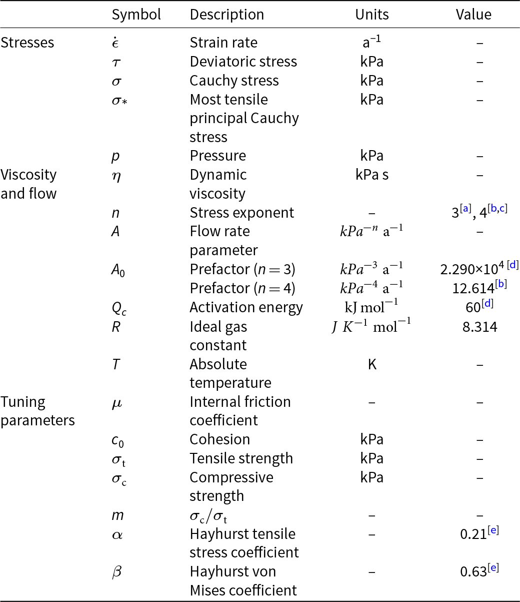
[a] Nye Reference Nye(1953); [b] Goldsby and Kohlstedt Reference Goldsby and Kohlstedt(2001); [c] Millstein and others Reference Millstein, Minchew and Pegler2022; [d] Duval and others Reference Duval, Ashby and Anderman(1983); [e] Pralong and Funk Reference Pralong and Funk2005.
We estimate stress states near ice fractures from observed strain rates, meaning the estimates of stress are dependent upon assumptions about ice rheology. Here, we calculate two sets of stress fields from the same strain rate data and apply the same criteria to each stress field to compare how assumed rheology changes estimated tensile strength. We define one stress field using n = 3 and tabulated A values from Cuffey and Paterson Reference Cuffey and Paterson2010, and the other using n = 4 and tabulated A values from Goldsby and Kohlstedt Reference Goldsby and Kohlstedt(2001). We assume a constant coefficient A 0 for each n value for the prefactor A. This simplification does not explicitly account for the effects of ice fabric (Staroszczyk and Morland, Reference Staroszczyk and Morland2001; Pettit and others, Reference Pettit, Thorsteinsson, Jacobson and Waddington2007; Hruby and others, Reference Hruby, Gerbi, Koons, Campbell, Martín and Hawley2020), grain size (Ranganathan and others, Reference Ranganathan, Minchew, Meyer and Peč2021b), ice damage (Borstad and others, Reference Borstad2012; Minchew and others, Reference Minchew, Meyer, Robel, Gudmundsson and Simons2018; Lhermitte and others, Reference Lhermitte2020), and other factors. We specifically choose to analyze areas where the variability of A due to damage is likely to be small, such as away from shear margins and large crevasse fields. Outside of shear margins, ice fabric causes a maximum factor of 2–3 variability in the value of A, which translates to a variability in viscosity, and thus calculated stress (Eqn 4), of ∼1.3 for n = 4 to 1.4 for n = 3 (Hudleston, Reference Hudleston2015). Spatial variations in the observed strain rates (Fig. 2) indicate that there should be no systematic nor homogeneous fabrics across the ice shelves, meaning that the effective fabric induced variations on A will vary between 1 and 3 in a way that will appear random in principle stress space, where we do the calibrations. Given that A is raised to the power  $-1/n$ in the expression for viscosity (and thus the calculation of stress), the maximum influence of fabric on our calculations of stress vary from 1.3 (for n = 4) to 1.4 (for n = 3), meaning that the influence of fabrics in our data will vary between 1 and 1.3 or 1.4 depending on the value of n. Thus, errors in A within our study area are a minor source of error relative to other uncertainties, and in the interest of simplicity, reproducibility and broader applicability of this work, we do not attempt to explicitly account for fabric. We leave for future work addressing the open question of how to reliably incorporate the effects of fabric into estimates of the strength of ice (Ma and others, Reference Ma, Gagliardini, Ritz, Gillet-Chaulet, Durand and Montagnat2010; Minchew and others, Reference Minchew, Meyer, Robel, Gudmundsson and Simons2018).
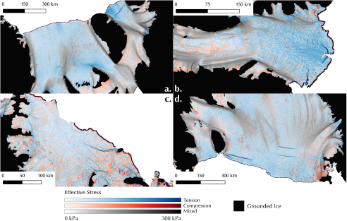
Figure 2. A view of stress regimes on the (a) Ronne–Filchner, (b) Amery, (c) Larsen C, and (d) Ross ice shelves. Black represents grounded ice (Morlighem, Reference Morlighem2019), blue represents a tensile regime (both principal Cauchy stresses are positive), red represents a compressive regime (both principal Cauchy stresses are negative), and gray represents a mixed regime (one principal Cauchy stress is positive and the other is negative). These colors correspond to the background colors in Figure 3. Each color is scaled by the effective deviatoric stress (assuming n = 3), with lighter colors representing lower stresses. The mixed, tensile, and compressive regimes cover 41.1%, 45.0% and 13.9% of all ice shelves, respectively.
While we calculate the deviatoric stresses from observed strain rates and Glen’s Flow Law (Eqns 3 and 4), yield criteria are often referenced to the Cauchy (or total) stresses, here denoted σij. The deviatoric and Cauchy stresses are related through the isotropic pressure (the mean of the normal Cauchy stresses) such that
 \begin{equation}
\tau_{ij} = \sigma_{ij} - p\delta_{ij}
\end{equation}
\begin{equation}
\tau_{ij} = \sigma_{ij} - p\delta_{ij}
\end{equation} where  $p = \sigma_{kk}/3$ is the pressure, σkk is the trace of the Cauchy stress tensor (summation implied for repeated indices), and δij is the Kronecker delta. The trace is the first tensor invariant; thus, the principal Cauchy stresses follow the same definitions and conventions discussed above for the strain rates and deviatoric stresses. Because shear stresses at the surface of the ice are negligible, one principal stress must be normal to the surface. We take the principal stress normal to the surface to be $\sigma_3 = -\rho g z$. At the surface of the ice, z = 0, thus $\sigma_3 = 0$, and we can calculate the principal Cauchy stresses at the ice surface from the observationally inferred deviatoric stresses as
 \begin{align}
\sigma_1 &= 2\tau_1 + \tau_2
\end{align}
\begin{align}
\sigma_1 &= 2\tau_1 + \tau_2
\end{align} \begin{align}
\sigma_2 &= 2\tau_2 + \tau_1
\end{align}
\begin{align}
\sigma_2 &= 2\tau_2 + \tau_1
\end{align} recalling that  $\tau_3 = -\tau_1-\tau_2$ by definition (cf. Eqn 7). The pressure at the surface is then
 \begin{align}
p &= \frac{\sigma_1 + \sigma_2}{3}
\end{align}
\begin{align}
p &= \frac{\sigma_1 + \sigma_2}{3}
\end{align} \begin{align}
&= \tau_1 + \tau_2.
\end{align}
\begin{align}
&= \tau_1 + \tau_2.
\end{align}2.3. Yield criteria
To determine the tensile and compressive strengths of ice, we plot our inferred stresses in principal deviatoric stress space and fit our data with a selection of yield criteria to delineate the boundary between stresses in uncrevassed and crevassed ice. Yield criteria, also known as failure envelopes, fracture criteria, failure criteria, etc., are bounds defined by material properties that delineate stresses past which failure should occur. In this work, we define yielding and failure as the conditions under which ice fractures and interchange the above terms. Here, we consider fracture to be a phenomenological description of the formation of new surfaces, not a description of the specific mechanisms that create those surfaces (i.e. we do not distinguish between brittle and ductile fracture). We choose the criteria given by Vaughan Reference Vaughan(1993)—Mohr–Coulomb, strain-energy dissipation, and von Mises criteria—plus the Drucker–Prager and Hayhurst criteria.
2.3.1. Mohr–Coulomb
The Mohr–Coulomb criterion was originally defined for and is commonly used to describe the yield strength of granular materials like soils and till (Lambe and Whitman, Reference Lambe and Whitman1969; Davis and Selvadurai, Reference Davis and Selvadurai2002). The basis of the Mohr–Coulomb criterion is the assumption that the strength of materials arises from a combination of internal friction and cohesion. A related criterion, the Tresca criterion, is a special case where internal friction is negligible and has been applied in the glaciological literature (Bassis and Walker, Reference Bassis and Walker2011). The opposite special case, where cohesion is negligible, is commonly used to describe the strength of subglacial till (e.g.
Iverson, Reference Iverson2010; Minchew and others, Reference Minchew2016; Zoet and Iverson, Reference Zoet and Iverson2020; Ranganathan and others, Reference Ranganathan, Minchew, Meyer and Gudmundsson2021a). The Mohr–Coulomb criterion accounts for only the most tensile and most compressive principal stresses, neglecting the intermediate principal stress, and is often written in a form that relates the shear strength of a material τs to the effective pressure N (difference in overburden and water pressures) through two parameters representing cohesion c 0 and internal friction µ (Labuz and Zang, Reference Labuz and Zang2012), such that  $\tau_s = N\mu\,\, +\,\, c_0$. Applying Mohr’s Circle and assuming the friction coefficient is small (i.e. $\mu = \tan{\phi} \approx \sin{\phi}$ where ϕ is the friction angle), we can write the Mohr–Coulomb criterion in terms of principal Cauchy stresses (Vaughan, Reference Vaughan1993) as
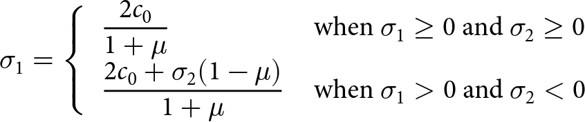 \begin{align}
\sigma_1 &= \left\{\begin{array}{l l}
\displaystyle \frac{2c_0}{1+\mu} & \text{when}\ \sigma_1 \ge 0\ \text{and}\ \sigma_2 \ge 0 \\
\displaystyle\frac{2c_0+\sigma_2(1-\mu)}{1+\mu} &
\text{when}\ \sigma_1 \gt 0\ \text{and}\ \sigma_2 \lt 0
\end{array}\right.
\end{align}
\begin{align}
\sigma_1 &= \left\{\begin{array}{l l}
\displaystyle \frac{2c_0}{1+\mu} & \text{when}\ \sigma_1 \ge 0\ \text{and}\ \sigma_2 \ge 0 \\
\displaystyle\frac{2c_0+\sigma_2(1-\mu)}{1+\mu} &
\text{when}\ \sigma_1 \gt 0\ \text{and}\ \sigma_2 \lt 0
\end{array}\right.
\end{align}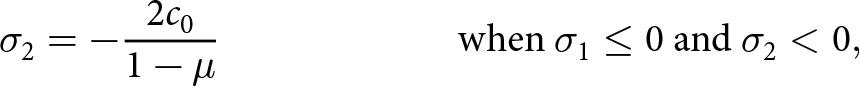 \begin{align}
\sigma_2 &= -\frac{2c_0}{1-\mu}
\qquad\qquad\qquad \text{when}\ \sigma_1 \le 0\ \text{and}\ \sigma_2 \lt 0,
\end{align}
\begin{align}
\sigma_2 &= -\frac{2c_0}{1-\mu}
\qquad\qquad\qquad \text{when}\ \sigma_1 \le 0\ \text{and}\ \sigma_2 \lt 0,
\end{align} from which we can see that the tensile strength for the Mohr–Coulomb criterion  $\sigma_{t_\mathrm{mc}}$, the compressive strength $\sigma_{c_\mathrm{mc}}$ and their ratio $m_\mathrm{mc}=\sigma_{c_\mathrm{mc}}/\sigma_{t_\mathrm{mc}}$ are
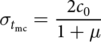 \begin{align}
\sigma_{t_\mathrm{mc}} &= \frac{2c_0}{1+\mu}
\end{align}
\begin{align}
\sigma_{t_\mathrm{mc}} &= \frac{2c_0}{1+\mu}
\end{align}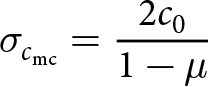 \begin{align}
\sigma_{c_\mathrm{mc}} &= \frac{2c_0}{1-\mu}
\end{align}
\begin{align}
\sigma_{c_\mathrm{mc}} &= \frac{2c_0}{1-\mu}
\end{align} \begin{align}
m_\mathrm{mc} &= \frac{1+\mu}{1-\mu}.
\end{align}
\begin{align}
m_\mathrm{mc} &= \frac{1+\mu}{1-\mu}.
\end{align}We can see in Eqn 11 that the Tresca criterion (µ = 0) requires the tensile and compressive strengths of ice to be equal (m = 1), a condition that is contradicted by numerous laboratory experiments (Petrovic, Reference Petrovic2003; Schulson and Duval, Reference Schulson and Duval2009) but nonetheless tested with our results.
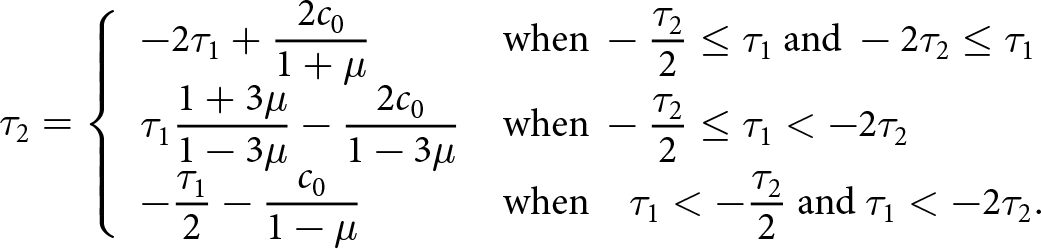
To connect with the observationally inferred deviatoric stresses, we apply Eqn 8 to write Eqn 10 in terms of the principal deviatoric stresses arranged as the standard equation for a line (with τ 1 the x-axis and τ 2 the y-axis) such that
 \begin{align}
\tau_2 = \left\{\begin{array}{l l} \displaystyle
-2\tau_1 + \frac{2c_0}{1+\mu} & {\displaystyle \text{when}\ -\frac{\tau_2}{2}\le\tau_1\ \text{and}\ -2\tau_2\le\tau_1} \\ \displaystyle
\tau_1\frac{1+3\mu}{{1-3\mu}} - \frac{2c_0}{1-3\mu} &
{\displaystyle \text{when}\ -\frac{\tau_2}{2} \le \tau_1 \lt -2\tau_2} \\ \displaystyle
-\frac{\tau_1}{2} - \frac{c_0}{1-\mu} & {\displaystyle \text{when}\ \phantom{-} \tau_1 \lt -\frac{\tau_2}{2}\ \text{and}\ \tau_1 \lt -2\tau_2}.
\end{array}\right.\nonumber\\
\end{align}
\begin{align}
\tau_2 = \left\{\begin{array}{l l} \displaystyle
-2\tau_1 + \frac{2c_0}{1+\mu} & {\displaystyle \text{when}\ -\frac{\tau_2}{2}\le\tau_1\ \text{and}\ -2\tau_2\le\tau_1} \\ \displaystyle
\tau_1\frac{1+3\mu}{{1-3\mu}} - \frac{2c_0}{1-3\mu} &
{\displaystyle \text{when}\ -\frac{\tau_2}{2} \le \tau_1 \lt -2\tau_2} \\ \displaystyle
-\frac{\tau_1}{2} - \frac{c_0}{1-\mu} & {\displaystyle \text{when}\ \phantom{-} \tau_1 \lt -\frac{\tau_2}{2}\ \text{and}\ \tau_1 \lt -2\tau_2}.
\end{array}\right.\nonumber\\
\end{align} Here, we can see that for the intermediate condition (when  $\sigma_1 \gt 0$ and $\sigma_2 \lt 0$ and, equivalently, $-\tau_2 \le 2\tau_1 \lt -4\tau_2$), the slope of the line is a function of only the internal friction coefficient µ while the y-intercept (taking τ 2 to be the y-axis) is a function of the cohesion, c 0, and the internal friction coefficient. For the other two conditions, the lines have a constant slope with y-intercepts that depend on cohesion and internal friction. Thus, taking all three regions given in Eqn 12, we can fit both c 0 and µ. We also note that the first and last conditions in Eqn 12 contain two separate inequalities for τ 1 in terms of τ 2 because the principal deviatoric stresses can be positive, negative and zero valued; the only restriction is our chosen convention $\tau_1\ge\tau_2$.
2.3.2. von Mises and strain energy
The von Mises criterion is a yield-stress-based parameterization of the rate of work done to deform a ductile material, as we later show. In practice, this criterion defines the tensile yield strength of materials in terms of a critical value of the stress, which is closely related to the effective deviatoric stress, τE (Eqn 5b). In three dimensions, the von Mises stress,  $\sigma_\mathrm{vm}$ is
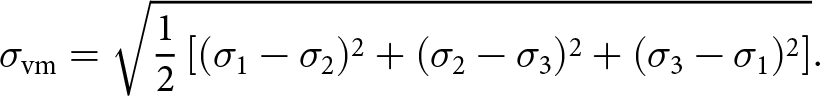 \begin{equation}
\sigma_\mathrm{vm}=\sqrt{\frac{1}{2}\left[(\sigma_1-\sigma_2)^2+(\sigma_2-\sigma_3)^2+(\sigma_3-\sigma_1)^2\right]}.
\end{equation}
\begin{equation}
\sigma_\mathrm{vm}=\sqrt{\frac{1}{2}\left[(\sigma_1-\sigma_2)^2+(\sigma_2-\sigma_3)^2+(\sigma_3-\sigma_1)^2\right]}.
\end{equation} As we are analyzing surface strain rates (z = 0), we take  $\sigma_3=-\rho gz=0$, and thus the von Mises stress at the surface is
 \begin{align}
\sigma_\mathrm{vm} &= \sqrt{\sigma_1^2 + \sigma_2^2 - \sigma_1 \sigma_2}
\end{align}
\begin{align}
\sigma_\mathrm{vm} &= \sqrt{\sigma_1^2 + \sigma_2^2 - \sigma_1 \sigma_2}
\end{align} \begin{align}
&= \sqrt{3}\tau_\mathrm{E}
\end{align}
\begin{align}
&= \sqrt{3}\tau_\mathrm{E}
\end{align} and the tensile strength of ice according to the von Mises criteria  $\sigma_{t_\mathrm{vm}}$ is the value of $\sigma_\mathrm{vm}$ that demarcates crevassed and uncrevassed ice.
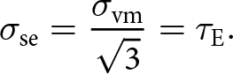
Because the von Mises criterion is a parameterization for the yield strength of materials as a work-rate threshold, it is essentially the same as the strain-energy dissipation criterion introduced by Vaughan Reference Vaughan(1993). In this criterion, the tensile strength of ice  $\sigma_{t_\mathrm{se}}$ is related to the rate of work: $\sigma_{ij}\dot{\epsilon}_{ij} = \tau_{ij}\dot{\epsilon}_{ij}$, where the replacement of the Cauchy stress tensor σij on the left-hand side with the deviatoric stress tensor τij on the right-hand side is justified by the incompressibility of ice (i.e. the pressure does not do work because the volume remains constant under applied stress). By applying Eqn 3, it can be shown that the stress associated with the viscous work rate (strain-energy dissipation) $\sigma_\mathrm{se}$ is proportional to the von Mises stress, $\sigma_\mathrm{vm}$, and, thus effective deviatoric stress $\tau_\mathrm{E}$, such that
 \begin{equation}
\sigma_\mathrm{se} = \frac{\sigma_\mathrm{vm}}{\sqrt{3}} = \tau_\mathrm{E}.
\end{equation}
\begin{equation}
\sigma_\mathrm{se} = \frac{\sigma_\mathrm{vm}}{\sqrt{3}} = \tau_\mathrm{E}.
\end{equation} The tensile strength from the Vaughan Reference Vaughan(1993) strain-energy dissipation criterion  $\sigma_{t_\mathrm{se}}$ is proportional to the tensile strength from the von Mises criterion such that $\sigma_{t_\mathrm{se}} = \sigma_{t_\mathrm{vm}}/\sqrt{3}$.
2.3.3. Drucker–Prager
The Drucker–Prager criterion links all of the previous criteria and provides a relatively simple framework, like the von Mises (and strain energy) criterion, that provides constraints on the tensile and compressive strengths of ice, like the Mohr–Coulomb criterion. In essence, the Drucker–Prager criterion is a smoothed form of the Mohr–Coulomb criterion, initially derived to describe the yielding of soil (Drucker and Prager, Reference Drucker and Prager1952). The criterion is dependent upon the first invariant of the Cauchy stress tensor (relatedly, pressure, p, Eqn 7) and the second invariant of the deviatoric stress tensor,  $\tau_\mathrm{E}$ (relatedly, the von Mises stress, $\sigma_\mathrm{vm}$, Eqn 14), and given as (Bhat and others, Reference Bhat, Choi, Wierzbicki and Karr1991; Davis and Selvadurai, Reference Davis and Selvadurai2002)
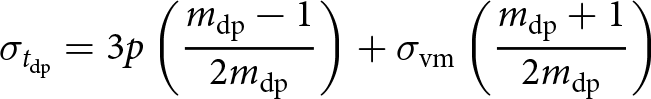 \begin{equation}
\sigma_{t_\mathrm{dp}} = 3p\left(\frac{m_\mathrm{dp}-1}{2m_\mathrm{dp}}\right) + \sigma_\mathrm{vm}\left(\frac{m_\mathrm{dp}+1}{2m_\mathrm{dp}}\right)
\end{equation}
\begin{equation}
\sigma_{t_\mathrm{dp}} = 3p\left(\frac{m_\mathrm{dp}-1}{2m_\mathrm{dp}}\right) + \sigma_\mathrm{vm}\left(\frac{m_\mathrm{dp}+1}{2m_\mathrm{dp}}\right)
\end{equation} where  $m_\mathrm{dp} = \sigma_{c_\mathrm{dp}}/\sigma_{t_\mathrm{dp}}$, $\sigma_{t_\mathrm{dp}}$ is the tensile strength and $\sigma_{c_\mathrm{dp}}$ the compressive strength according to the Drucker–Prager criterion. These values can be inferred by defining the failure envelope formed in principal stress space by Eqn 16 that delineates crevassed and uncrevassed ice. Because the Drucker–Prager criterion is a smoothed version of the Mohr–Coulomb criterion, we can relate the inferred strengths $\sigma_{t_\mathrm{dp}}$ and $\sigma_{c_\mathrm{dp}}$ to cohesion, c 0, and internal friction, µ, of ice by requiring that the Drucker–Prager failure envelope intersect the Mohr–Coulomb failure envelope at the latter’s major vertices, i.e. fully circumscribe the Mohr–Coulomb envelope. The resulting relations are
 \begin{align}
\sigma_{t_\mathrm{dp}} &= \frac{6c_0}{3+\mu}
\end{align}
\begin{align}
\sigma_{t_\mathrm{dp}} &= \frac{6c_0}{3+\mu}
\end{align}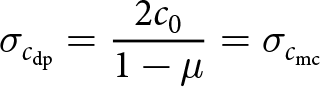 \begin{align}
\sigma_{c_\mathrm{dp}} &= \frac{2c_0}{1-\mu} = \sigma_{c_\mathrm{mc}}
\end{align}
\begin{align}
\sigma_{c_\mathrm{dp}} &= \frac{2c_0}{1-\mu} = \sigma_{c_\mathrm{mc}}
\end{align} \begin{align}
m_\mathrm{dp} &= \frac{3+\mu}{3\left(1-\mu\right)}
\end{align}
\begin{align}
m_\mathrm{dp} &= \frac{3+\mu}{3\left(1-\mu\right)}
\end{align}all of which reduce to the same values as in Eqn 11 when µ = 0 (the Tresca criterion). We also note that the relations between tensile strength, cohesion and friction differ for the Mohr–Coulomb and Drucker–Prager failure envelopes, but the compressive strength relation is the same. This agreement in compressive strength inexorably arises from our decision to have the Drucker–Prager envelope intersect the Mohr–Coulomb envelope at the major vertices. The relations will vary if we make different choices for the intersections of the Mohr–Coulomb and Drucker–Prager failure envelopes, but we stay with these relations for illustrative purposes because the major vertices provide unambiguous reference points.
2.3.4. Hayhurst
The Hayhurst criterion was first developed to describe the failure of metals and is commonly used in continuum damage mechanics models of ice fracture (Hayhurst, Reference Hayhurst1972; Pralong and Funk, Reference Pralong and Funk2005; Duddu and others, Reference Duddu, Jiménez and Bassis2020). It adds a term related to the most tensile principal Cauchy stress  $\sigma_* = \max{[\sigma_1,0}]$ to the Drucker–Prager criterion (Eqn 16), such that
 \begin{equation}
\sigma_\mathrm{t_H} = \alpha\sigma_* + \beta\sigma_\mathrm{vm} + 3(1-\alpha-\beta) p
\end{equation}
\begin{equation}
\sigma_\mathrm{t_H} = \alpha\sigma_* + \beta\sigma_\mathrm{vm} + 3(1-\alpha-\beta) p
\end{equation} where α and β are non-negative and  $0\le(1-\alpha-\beta)\le1$. We take
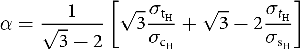 \begin{align}
\alpha &= \frac{1}{\sqrt{3}-2}\left[\sqrt{3}\frac{\sigma_\mathrm{t_{H}}}{\sigma_\mathrm{c_{H}}}+\sqrt{3}-2\frac{\sigma_{t_\mathrm{H}}}{\sigma_\mathrm{s_{H}}} \right]
\end{align}
\begin{align}
\alpha &= \frac{1}{\sqrt{3}-2}\left[\sqrt{3}\frac{\sigma_\mathrm{t_{H}}}{\sigma_\mathrm{c_{H}}}+\sqrt{3}-2\frac{\sigma_{t_\mathrm{H}}}{\sigma_\mathrm{s_{H}}} \right]
\end{align}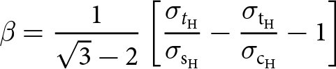 \begin{align}
\beta &= \frac{1}{\sqrt{3}-2}\left[\frac{\sigma_{t_\mathrm{H}}}{\sigma_\mathrm{s_H}}-\frac{\sigma_\mathrm{t_H}}{\sigma_\mathrm{c_H}}-1 \right]
\end{align}
\begin{align}
\beta &= \frac{1}{\sqrt{3}-2}\left[\frac{\sigma_{t_\mathrm{H}}}{\sigma_\mathrm{s_H}}-\frac{\sigma_\mathrm{t_H}}{\sigma_\mathrm{c_H}}-1 \right]
\end{align} as in Pralong and Funk Reference Pralong and Funk2005, where  $\sigma_\mathrm{t_H}$ is the tensile strength, $\sigma_\mathrm{c_H}$ is the compressive strength and $\sigma_\mathrm{s_H}$ is the shear strength. We solve both equations for the ratio m between compressive and tensile strength:
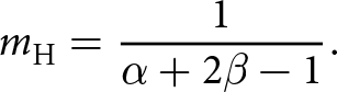 \begin{equation}
m_\mathrm{H}=\frac{1}{\alpha+2\beta-1}.
\end{equation}
\begin{equation}
m_\mathrm{H}=\frac{1}{\alpha+2\beta-1}.
\end{equation}The Hayhurst criterion (Eqn 18) reduces to the Drucker–Prager criterion (Eqn 16) when α = 0.
3. Results
3.1. Visualizing the conditions under which ice fractures
The goal of this work is to constrain the tensile strength of ice on Antarctic ice shelves. To do this, we look to see if there is a clear threshold in our data at which unfractured ice will fail. We plot the uncrevassed and crevassed data as density plots in principal deviatoric stress space, with the color of each point denoting the number of points in its proximity (Fig. 3). We find minimal overlap between the uncrevassed and crevassed data. Because there is no particular significance to the assignment of τ 1 and τ 2 in principal stress space, we reflect the data over the line  $\tau_1=\tau_2$ to aid in drawing yield criteria, as in Vaughan Reference Vaughan(1993)
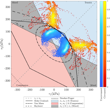
Figure 3. A density plot in principal stress space of estimated principal stresses (assuming n = 3) sampled along crevasses (red) and in uncrevassed areas (blue). Colorbars for the crevassed and uncrevassed data are scaled logarithmically and normalized, with brighter colors representing a higher density of points in the area. The yield criteria are plotted on top of the density plot using the best fit values of tensile strength in Table 2, with both the Drucker–Prager and Mohr–Coulomb criteria plotted with µ = 0.4. To aid in comparing principal stress space and geographic space, we shade each quadrant with the corresponding colors used for stress states in Figure 2. Colorblind-accessible figures are available in the supplement.
.
We identify no active crevasses that exist in a compressive regime (both principal Cauchy stresses are negative). Most ice shelves exist with a free calving front, which means it is unlikely for the system to be in a compressional state  $(\sigma_1,\sigma_2 \lt 0)$ because there is no resistive pressure from the ocean on the free calving front. There are localized observations of compressive fractures in rapidly changing areas such as the Thwaites Ice Tongue (Benn and others, Reference Benn2022), but the applicability of fractures caused by ice acceleration to the large, slow-growing fractures in this study needs further investigation. Even in unfractured ice, there are few regions that fall into a purely compressional regime, with such areas covering about 13.9% of all Antarctic ice shelves (Fig. 2). As such, we find relatively few uncrevassed points in the compressive regime compared to other regimes.
To find the tensile strength of ice, we plot the Mohr–Coulomb, von Mises, Drucker–Prager and Hayhurst criteria over our data and tune their fit using material properties such as cohesion, internal friction, and tensile strength. We aim to draw the criteria between the crevassed and uncrevassed data, minimizing the number of crevassed points included and maximizing the number of uncrevassed points included. The yield criteria are shown in Fig. 3. For the Drucker–Prager and Mohr–Coulomb criteria, we vary the values of µ and c 0 to fit the criteria. For the von Mises and Hayhurst criteria, we vary the values of  $\sigma_\mathrm{t}$ to find best fit. We do not investigate fit values for the strain-energy criterion, as the shape of the criterion is the same as that of the von Mises criterion, with tensile strength reduced by a factor of $\sqrt{3}$. We plot the Hayhurst criterion using empirically determined (i.e. calibrated through experiments) values of $\alpha=0.21,\;\beta=0.63$ (Pralong and Funk, Reference Pralong and Funk2005).
To analyze fit, we determine the percentage of uncrevassed and crevassed data points included in each criterion using a dataset of ∼11700 and ∼3500 points, respectively. For each criterion, we test for three scenarios of fit: (1) the highest integer value of the tuning parameter (c 0 or  $\sigma_\mathrm{t}$) where the criterion includes no crevassed data, (2) the integer value of the tuning parameter where the derivatives of percent uncrevassed and percent crevassed included with respect to the tuning parameter are equal, and (3) the lowest integer value of the tuning parameter where the criterion includes 100% of uncrevassed data. We define ‘best fit’ by the second scenario and use the other two scenarios to provide an upper and lower bound for the estimates of tensile strength produced by each criterion. Our low estimate of tensile strength encapsulates the error of crevasse advection out of stress states of crevasse formation, which is evidenced by the low percentage of uncrevassed points included in the criteria in the first scenario. While we aim to filter out inactive crevasses through our identification methodology, some may still be included in our data. Therefore, it is better to define criteria based on the current stress state of ice that remains unfractured rather than by excluding crevassed data, as noted by Vaughan Reference Vaughan(1993).
3.2. Tensile strength of ice
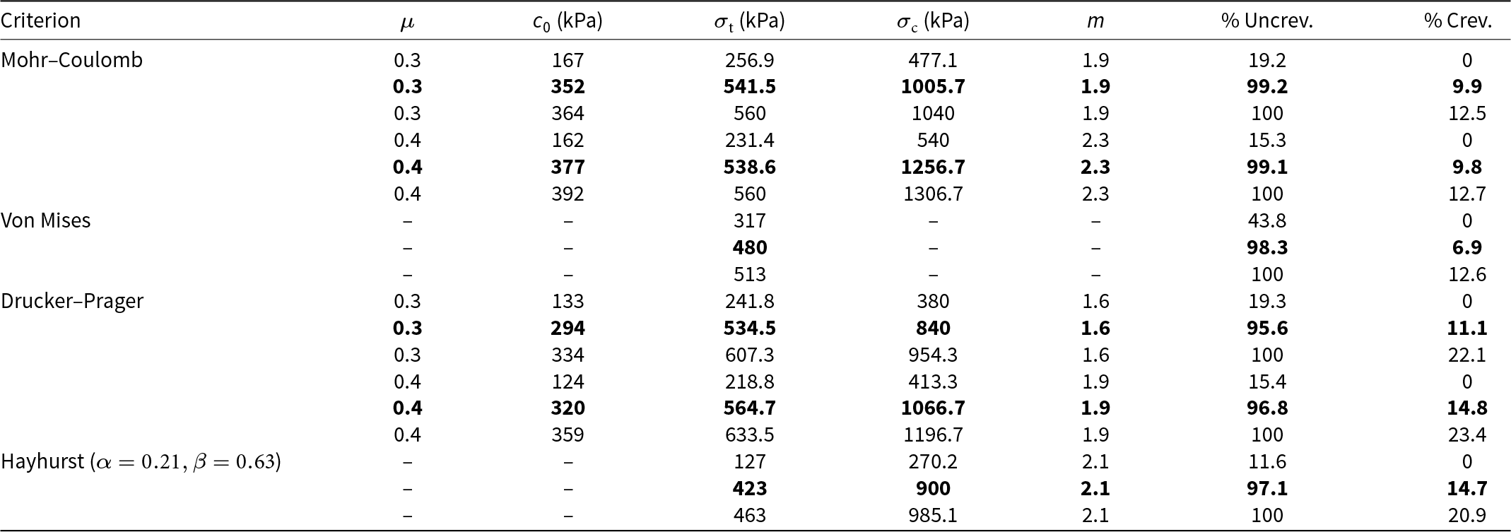
Using the above framework and the four selected yield criteria, we find the tensile strength of ice to range from 59 to 289.4 kPa when n = 3 and 127 to 633.5 kPa when n = 4. Under the best fit case, the tensile strength ranges from 202 to 263 kPa assuming n = 3 and 423 to 565 kPa assuming n = 4. The predicted tensile strengths increase by a factor of  $\sim 2.1$ between n = 3 and n = 4, although a larger percentage of crevassed points are included for criteria drawn around stresses calculated using n = 4. We present a selected range of tensile strengths in Tables 2 and 3 and include a full range of tensile strengths for varying $\sigma_\mathrm{t}$, c 0, and µ values in the supplement. We plot our best fit tensile strengths for the criteria in Fig. 3 and provide plots of criteria defined by the minimum and maximum tensile strengths in the supplement.
Table 2. Tested values of internal friction (µ), cohesion (c 0) and tensile strength (σt) used to fit the criteria to our stress data when  $\bf{n=3}$. Compressive strength (σc) is calculated from µ, c 0, and σt using the equations described in Section 2. For each criterion, we present a low, best fit (bolded), and high estimate of tensile strength as described in the text
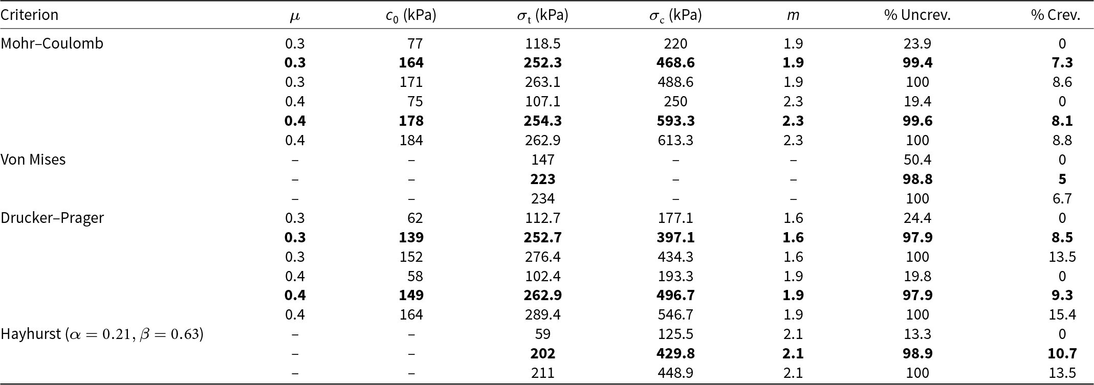
Table 3. Tested values of internal friction (µ), cohesion (c 0) and tensile strength (σt) used to fit the criteria to our stress data when  $\bf{n=4}$. Compressive strength (σc) is calculated from µ, c 0, and $\sigma_\mathrm{t}$ using the equations described in the methods. For each criterion, we present a low, best fit (bolded), and high estimate of tensile strength as described in the text
Under both assumed rheologies, the Mohr–Coulomb and von Mises criteria produce a more constrained range of tensile strength estimates and include minimal crevassed data compared to the other two criteria. When n = 3, the von Mises criterion has a difference of 87 kPa between low and high estimates for tensile stress, and the Mohr–Coulomb criterion produces a range of 49 kPa when µ = 0 and 109 kPa when µ = 0.4. Both criteria include less than 10% of the crevassed data under our highest estimates of tensile strength and  $\mu=0-0.7$. The Drucker–Prager criterion provides a smaller range of tensile strength values but includes more crevassed points than the Mohr–Coulomb and von Mises criteria, especially as µ increases. The Hayhurst criterion produces a range of 138 kPa between our low and high estimates of tensile strength and contains the largest percentage of crevassed points, including 13.5% of the crevassed points when 100% of the uncrevassed data are included.
4. Discussion
4.1. Toward a general fracture criterion
We evaluate the applicability of previously derived yield criteria to observations of ice fracture. The von Mises criterion (describing the failure of materials based on the second invariant of the deviatoric stress tensor) and the strain energy criterion (describing the failure of materials based on strain-energy dissipation) have been historically applied to the question of ice fracture (e.g. Vaughan (Reference Vaughan1993), Pralong and Funk (Reference Pralong and Funk2005), Albrecht and Levermann (Reference Albrecht and Levermann2012)). Using yield criteria, Vaughan Reference Vaughan(1993) evaluates the tensile strength in specific regions of Antarctica with a total of  $\sim 990$ strain-rate measurements. Vaughan Reference Vaughan(1993) finds the tensile strength to vary from 90 to 320 kPa and the von Mises and Mohr–Coulomb criteria to provide a good fit. This is comparable to the results of Grinsted and others Reference Grinsted, Rathmann, Mottram, Solgaard, Mathiesen and Hvidberg2024, who finds a von Mises strength of $265\pm73$ kPa. We similarly find the von Mises and Mohr–Coulomb criteria to fit the data well, and our predicted tensile strength range of 202–263 kPa (assuming n = 3) falls within the upper end of the values predicted by Vaughan Reference Vaughan(1993) and Grinsted and others Reference Grinsted, Rathmann, Mottram, Solgaard, Mathiesen and Hvidberg2024, both of whom only consider stresses calculated with n = 3. Our predicted range of 423–565 kPa for n = 4 falls more than 100 kPa outside the upper bound of Vaughan’s range, although it is much closer to the range predicted by laboratory experiments (Petrovic, Reference Petrovic2003).
Vaughan Reference Vaughan(1993) provides a 230 kPa range of tensile strengths, while our predicted tensile strengths produce a range of 61 and 142 kPa for n = 3 and n = 4, respectively. Our narrower predicted ranges are likely due to the increased amount of data available for our study. Satellites have proved pivotal for increasing the spatial and temporal resolution of strain rate measurements, allowing us to collect a sample size of  $\sim14500$ crevassed and uncrevassed data points. While our sample size of crevassed data is limited by the number of crevasses visible on optical imagery and strain rate data, the $\sim11000$ uncrevassed points are a small subsection of the data available for uncrevassed ice.
We find that the von Mises and Mohr–Coulomb criteria provide the best numerical fit to our data. Best numerical fit means the range of inferred tensile strength values is small and few crevassed points are inside the failure envelope. The Drucker–Prager criterion provides a good fit to the data when  $\mu\le0.3$. When µ = 0, the Drucker–Prager criterion reduces to the von Mises criterion and produces virtually identical values of predicted tensile strength (Supplement Table S2). While the Hayhurst criterion provides the poorest numerical fit to our data relative to all other criteria, it aligns well with the data in pure tension. It mostly includes crevassed data in the mixed regime. As many fractures occur in pure tension, the Hayhurst criterion still provides a viable framework for understanding damage evolution in this regime. Further work is necessary to determine the applicability of the Hayhurst criterion to damage and failure in shear regimes, though we expect the broad takeaways to hold because failure in shear zones often occurs in tension.
It is particularly interesting to consider the pressure dependencies of the fracture criteria with regard to their fit. Numerically, the von Mises criterion provides the best fit to the data. This criterion is also the only criterion of those tested that is not pressure-dependent. We postulate that the von Mises criterion fits so well because we consider stresses only at the surface, where the overburden pressure equals the vertical normal stress  $\sigma_3 = 0$. A von Mises criterion defined by our estimated tensile strengths from surface crevasses will likely not fit well for basal crevasses since the criterion predicts the same tensile strength for all depths. Overburden pressure ( $\sigma_3 = -\rho g z$) will act against crevasse formation at increasing depths. Thus, observations of stresses surrounding basal crevasses are needed to properly constrain failure at depth. By estimating stresses around basal crevasses, it may be possible to refine our results to a single fracture criterion that fits data through the entire thickness of the ice.
We find the Drucker–Prager and Mohr–Coulomb criteria numerically fit best with lower values of µ. Other studies also find models better replicate observations when using lower values of µ (MacAyeal and others, Reference MacAyeal, Shabtaie, Bentley and King1986; Bassis and Walker, Reference Bassis and Walker2011). However, a low value of µ corresponds to a low ratio between tensile and compressive strength. When µ = 0, the equations for compressive strength derived from the yield criteria (Eqn 11 and 17) suggest the tensile and compressive strengths are equal, a phenomenon that is not observed in most natural materials. For example, rocks commonly have µ values of 0.5–0.7 (Byerlee, Reference Byerlee, Byerlee and Wyss1978), leading to compressive strengths 2.3–5.7 times higher than the tensile strength. The compressive strength of ice in the lab has been measured between 5 and 25 MPa, far greater than lab measurements of the tensile strength (Petrovic, Reference Petrovic2003). The lack of observable crevasses in compressive ice regimes also points to the compressive strength of ice being greater than the tensile strength. In this work, we choose to present tensile strength ranges for the Drucker–Prager and Mohr–Coulomb criteria defined by  $\mu=0.3-0.4$, in spite of the fact that lower µ values fit better numerically, due to the implications of µ on the predicted compressive strength of ice. We provide a full list of tensile strengths for each criterion defined by $\mu=0-0.7$ in the supplement.
One important limitation of our study arising from the lack of appropriate data is our inability to constrain the strength of ice for the nucleation of new fractures. The data we use only allow us to constrain the strength of ice that is relevant for fracture propagation. The key difference between nucleation and propagation is the preexisting flaw sizes. We might assume that for a given fracture toughness, we can simply scale ice strength as the square root of the flaw size (Schulson and Duval, Reference Schulson and Duval2009), but this assumption remains to be tested in natural glacier ice, where impurities and air bubbles can play important roles. This limitation provides opportunities, and perhaps impetus, for collecting and testing this assumption with relevant data but does not undercut the value of providing constraints on the conditions for fracture propagation, as we do here.
4.2. Predicting fracture
Using the best-fit values for tensile strength and n = 4, as described in Table 3, we create a map of areas that fall outside of the yield criteria (i.e. the ice should be fractured) on all Antarctic ice shelves (Figs 5 and 6). We find our predicted tensile strengths work well for predicting large-scale fractures, and areas where stresses fall under the yield threshold generally do not show signs of active crevassing. The predicted fracture map picks up some fractures, particularly on the Amery Ice Shelf near a portion of isolated grounded ice on the eastern margin, that do appear on both optical imagery and the strain rate fields but were not included in our original analysis due to their proximity to the shear margin and a large chain of crevasses, which could introduce uncertainties in rheology associated with damage.

Figure 5. A map of predicted fracture areas for n = 4 on the (a) Ronne–Filchner, (b) Amery, (c) Larsen C, and (d) Ross Ice Shelves. White represents areas where all four yield criteria predict the ice will fracture, and dark gray represents areas where no criteria predict fracture will occur.
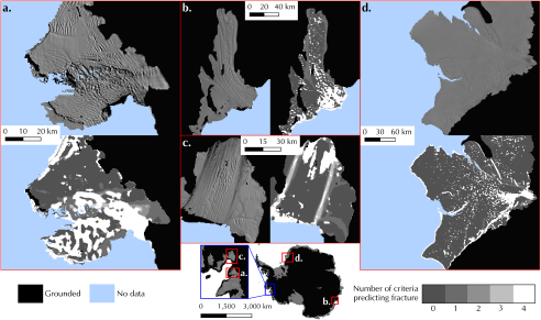
Figure 6. MODIS 2014 imagery (top [a,d]; left [b,c]) and our predicted fracture map (bottom [a,d]; right [b,c]) of four smaller ice shelves originally outside of the study area: (a) Thwaites, (b) Totten, (c) Pine Island and (d) Brunt.
The primary difference in predictions between the four criteria is in shear zones. The von Mises criterion predicts fracture in shear zones whereas all other criteria (assuming µ = 0.4) predict no fracture in these areas. For the Drucker–Prager and Mohr–Coulomb criteria, lower values of µ predict more fracturing in shear zones, and the area of predicted shear zone fracturing decreases as µ increases. The main areas where the predicted fracture map is inaccurate to observations are toward the calving front of the Amery and Filchner ice shelves and in front of a large upstream section of grounded ice on the Ronne Ice Shelf, where all criteria predict heavy fracturing but none is visible on optical imagery. There may be other rheological factors influencing the strength of ice in these areas, such as suture zones, differences in ice thickness and temperature, or other parameters that require further study. We also note that the speckled patterns of predicted fracture close to Ross Island on the RIS, on the parts of the LCIS, and downstream of the aforementioned predicted fracture zone on the Ronne Ice Shelf are likely due to noise in the strain rate data, as we see very few surface expressions of any crevasses, relict or active, in these areas. As observations improve in the future, we expect to be able to better resolve these areas.
In addition to analyzing the predicted fracture map over the original study area, we also investigate the accuracy of the map over four smaller ice shelves: the Thwaites, Totten, Pine Island, and Brunt ice shelves (Fig. 6). On these smaller ice shelves, we observe smaller and more densely packed fractures. Our predicted fracture map is not as robust in predicting the locations of individual fractures on these ice shelves due to the large spatial resolution of the strain rate fields relative to the size of the ice shelves and fractures but does predict where the ice shelves tend to be intact versus where they are heavily fractured. The fracture prediction map shows heavy fracturing on the Western Ice Tongue of Thwaites, while it shows the Eastern Ice Shelf more intact, matching surface observations of damage in the area, although the map does fail to predict several large rifts that have visible surface expressions. On the Brunt Ice Shelf, the von Mises criterion predicts fracturing in a compressive region around the upstream end of the McDonald Ice Rumples, an area where no other criteria predict fracturing but where smaller fractures are observed. On the Pine Island Ice Shelf (PIIS), all criteria predict some level of fracturing in the shear margins and just downstream of the grounding zone, but fractures are not observed in these locations. This incorrect fracture prediction could be related to rheological differences associated with a high deformation rate, as Pine Island Glacier is one of the fastest flowing glaciers in Antarctica and thus experiences high strain rates in the shear margins (Rignot, Reference Rignot2008). The Hayhurst criterion predicts the least amount of fracturing in the PIIS shear margins, although it still predicts some fracturing, particularly along the Southern shear margin. The predicted fracture map does accurately capture with all four criteria a relatively large ( $\sim 7\mathrm{km}$) fracture in the middle of the PIIS, which eventually calves off a tabular iceberg in late 2015. The accuracy of the map in regions that were not included in the construction of the fracture criteria suggests that the map and predicted tensile strengths could be used in transient ice flow models to predict areas where large fractures may form or the extent of damage on smaller ice shelves.
4.3. Applicability to modeling efforts
Our framework produces a range of tensile strengths for each yield criterion and two different flow regimes based on how we define the fit to the data. These values are presented in Tables 2 and 3 and further expanded in the supplement. In general, ice with active crevasses exists at higher stresses than unfractured ice (Fig. 2). We aim to give a broad understanding of how different definitions of fit may influence the range of tensile strengths produced. Therefore, these results produce a constrained range of tensile strengths, rather than a single value. The strength of ice is also likely to vary spatially based on rheological properties, and our data likely capture this range (Schulson and Duval, Reference Schulson and Duval2009).
Given the quantity of data now available and the fact that we can produce continent-wide estimates of tensile strength, we believe that these results could extend beyond providing single tensile strength values to be used as fracture criteria in models. The range of tensile strength values could be thought of as uncertainty bounds that can be input into stochastic models, rather than a set threshold for fracture, to take into account the variability in the strength of ice with varying material properties. Additionally, the percentage of uncrevassed and crevassed points included in the criteria (e.g. Fig. 4) can provide constraints on a probability distribution function. This may allow us to ask questions in a probabilistic sense, such as what is the probability of ice fracture at certain principal stresses?
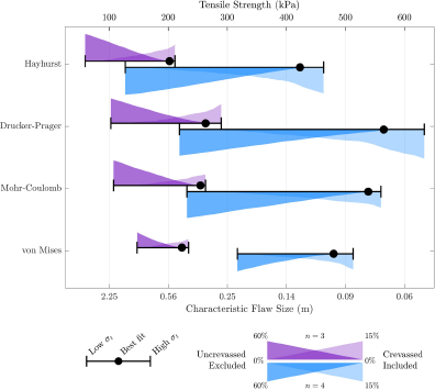
Figure 4. The range of tensile strengths produced by each criterion under our framework. Error bars represent our minimum and maximum estimates for tensile strength, and our best fit case is plotted as a black dot. The height of the shaded area on top of/beneath the error bar denotes the percent of uncrevassed points excluded (dark purple/blue) and percent of crevassed points included (light purple/blue) by a criterion defined by that tensile strength for n = 3 and n = 4, respectively. For the Mohr–Coulomb and Drucker–Prager criteria, we plot the values for a criterion defined by µ = 0.4. A plot of the full range of µ values is available in the supplement. The characteristic flaw size associated with each tensile strength, calculated assuming  $K_{Ic}=150\;kPa\;m^{-1/2}$, is plotted on the bottom axis.
Additionally, our methodology can be used to determine the regional strength of ice. Because we see very minimal overlap between the crevassed and uncrevassed data, it is possible to define an upper bound for ice strength solely from uncrevassed data. As noted previously, Vaughan Reference Vaughan(1993) defined yield criteria by including all uncrevassed points rather than excluding crevassed points. Regional tensile strengths can be derived from looking at the upper bound of uncrevassed stresses in areas without crevasses. In future work, we hope to explore the strength of suture zones and how they interact with crevasse propagation. Constraining the different rheological properties affecting tensile strength and how they vary spatially across Antarctica is important for accurately modeling fracture formation, propagation, and iceberg calving.
4.4. Implications for damage
In this work, we present estimates for a stress threshold at which ice fractures initiate and propagate on a large-scale. This can also be interpreted as the tensile strength of ice (that is, the maximum stress ice can withstand under tension before fracturing). These estimates can also illuminate some material properties of the ice itself.
The tensile strength of ice is dependent upon a number of physical properties, including ice temperature and grain size (Schulson and others, Reference Schulson, Lim and Lee1984; Cole, Reference Cole1987; Nixon and Schulson, Reference Nixon and Schulson1987; Schulson and Duval, Reference Schulson and Duval2009). Therefore, the estimates of ice strength presented in this study can provide constraints on the characteristic flaw size of glacier ice. Ice grain size can be considered the characteristic flaw size of undamaged ice. Since grain boundaries are irregular bonds connecting two ice grains, grain boundaries are inherently the smallest flaw in glacier ice (Schulson and Hibler, Reference Schulson and Hibler1991).
The relationship between the tensile strength of ice  $\sigma_\mathrm{t}$ and characteristic flaw size d has been determined through laboratory experiments to be (Currier and Schulson, Reference Currier and Schulson1982; Schulson and others, Reference Schulson, Lim and Lee1984)
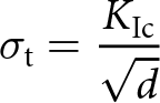 \begin{align}
\sigma_\mathrm{t} = \frac{K_\mathrm{Ic}}{\sqrt{d}}
\end{align}
\begin{align}
\sigma_\mathrm{t} = \frac{K_\mathrm{Ic}}{\sqrt{d}}
\end{align} where  $K_\mathrm{Ic}$ is the Mode I (tensile) fracture toughness of ice (Nixon and Schulson, Reference Nixon and Schulson1988). The fracture toughness of ice has been experimentally determined to be within the range of 50–150 $\mathrm{kPa}\sqrt{\mathrm{m}}$ (Petrovic, Reference Petrovic2003).
The estimates of tensile strengths presented in this study imply large characteristic flaw sizes d, with d ≈ 4–36 cm assuming n = 3 ( $\sigma_\mathrm{t} \approx 250$ $\mathrm{kPa}$) and $d\approx1-9$ cm assuming n = 4 ( $\sigma_\mathrm{t} \approx 500$ $\mathrm{kPa}$). The characteristic flaw size estimates for both n = 3 and n = 4 are an order of magnitude larger than the typical grain sizes of glacier ice (on the order of millimeter scale), although the n = 4 estimates are much closer to observed grain sizes (Gow and others, Reference Gow1997; Thorsteinsson and others, Reference Thorsteinsson, Kipfstuhl and Miller1997; Fitzpatrick and others, Reference Fitzpatrick2014; Gerbi and others, Reference Gerbi2021, Ranganathan and others, Reference Ranganathan, Minchew, Meyer and Peč2021b). The value of d can be interpreted as the maximum flaw size within the ice that can be considered ductile. At flaw sizes (or microcracks) larger than these estimated values of d, cracks will become unstable and propagate (Schulson and Duval, Reference Schulson and Duval2009).
4.5. Reconciling ice strength and ice viscosity
Notably, the regions in which we map fractures on Antarctic ice shelves overlap strongly with regions in which the stress exponent is estimated to be n = 4 based on observations (Millstein and others, Reference Millstein, Minchew and Pegler2022), suggesting that dislocation creep is the dominant mechanism of deformation. These are regions in which the along-flow (normal) deviatoric stress is in tension and proportional to the local ice thickness (Millstein and others, Reference Millstein, Minchew and Pegler2022). This has two implications.
Firstly, it suggests that the values of tensile strength we estimate from n = 4 are likely most applicable in those regions. Historically, stresses have been calculated using n = 3, a value used in the literature from the early 1960s onward, derived from a combination of laboratory experiments and field measurements (Glen, Reference Glen1952, Reference Glen1955, Reference Glen1958; Nye and Perutz, Reference Nye and Perutz1957; Haefeli, Reference Haefeli1961; Lliboutry, Reference Lliboutry1968). However, recent studies have shown that in Antarctica and specifically on the fast-flowing Antarctic ice shelves, the value of n for ice should be closer to 4 (Goldsby and Kohlstedt, Reference Goldsby and Kohlstedt2001; Cuffey and Kavanaugh, Reference Cuffey and Kavanaugh2011; Bons and others, Reference Bons2018; Millstein and others, Reference Millstein, Minchew and Pegler2022; Ranganathan and Minchew, Reference Ranganathan and Minchew2024). We find the tensile strength of ice is ∼2.1 times greater when assuming n = 4 compared to n = 3. While our results do not aim to constrain the value of n, we do note that tensile strength estimates for n = 4 are much closer to those produced by laboratory experiments than previous observational studies (Vaughan, Reference Vaughan1993; Petrovic, Reference Petrovic2003; Chudley and others, Reference Chudley2021; Grinsted and others, Reference Grinsted, Rathmann, Mottram, Solgaard, Mathiesen and Hvidberg2024). Additionally, the lower tensile stress estimates of an n = 3 flow regime produce larger characteristic flaw size estimates.
Secondly, the presence of crevasses in these tensile areas in which n = 4 is the observed estimate of the stress exponent indicates that the tensile stresses in these areas are larger than the tensile strength estimated in this work, begging the question: Why is it common to find viscous stresses in the ice shelves that are high enough to meet the fracture criteria? This suggests common mechanisms link viscosity and fracture strength, such as dislocations (Weertman, Reference Weertman1996). Given recent inferences of the viscous stress exponent n = 4, which laboratory studies show arises from dislocation creep (Goldsby and Kohlstedt, Reference Goldsby and Kohlstedt2001), and the fact that fractures are made up of dislocations aligned to form a surface (Weertman, Reference Weertman1996), we suppose that the rapid formation and mobilization of dislocations required to allow for dislocation-creep-dominated viscous flow creates a work-hardening effect that leads to microcracks and eventually macro-scale fractures. Such a mechanism could also explain why ice fractures lead to large-scale rift formation even though it takes months to years to build up enough stress in the ice for some rifts to propagate (Borstad and others, Reference Borstad, McGrath and Pope2017). This observation of episodic rift propagation, where the time between episodes is much longer than the viscoelastic relaxation time, is mysterious because when the viscous stress exponent has values of n = 3–4, the viscosity should tend to zero as the stresses intensify around the rift tip. Intuition suggests that ice should relieve these stresses through viscous flow, yet rifts propagate as fractures. Our observations of the alignment of tensile strength and viscosity of ice and the hypothesis that dislocations are responsible for both viscous flow and fracture on ice shelves could explain episodic rift formation, too, and help to reconcile our understanding of the flow, deformation and fracture of ice.
5. Conclusion
We use observations of ice fractures and estimated stresses to evaluate the tensile strength of ice. We produce a map of observed fractures in 2014 over four major Antarctic ice shelves and a range of tensile strengths for stresses calculated with both n = 3 and n = 4. We find a tensile strength value between 202 and 263 kPa assuming n = 3, on the higher end of previous observational estimates but still lower than experimentally derived tensile strengths. When n = 4, the predicted tensile strength is 423–565 kPa. We produce a map of predicted fracturing across all Antarctic ice shelves using these values.
Our predicted tensile strengths when n = 4 are within the lower bound,  $\sim500$ kPa, of tensile strength estimates produced by laboratory experiments. Previous observational studies assuming n = 3 have predicted tensile strengths of $\sim100$–300 kPa or about 200 kPa below the lower bound of laboratory estimates. With the inclusion of impurities and damage in natural glacier ice, observationally inferred tensile strength estimates are likely to be lower than those measured in pristine laboratory ice. Damage must be extensive and pervasive to account for such a large difference between lab estimates and these observationally derived tensile strengths. We hypothesize that assuming n = 4 rather than n = 3 accounts for most of this discrepancy, as evidenced by our n = 4 tensile strength estimates aligning with laboratory studies. This alignment in observed versus measured strength values brings us one step closer to bridging the gap between experiments and observations, allowing us to better apply material properties of ice measured in lab environments to naturally deforming glacier ice.
Ice rheology plays a central role in this work, both from the perspective of inferences of stress and how our results inform a deeper understanding of the mechanical properties of natural glacier ice. The viscous rheology of ice appears most prevalently as the stress exponent, n, and the corresponding prefactor A in Glen’s Flow Law. The influence of our choices of n on the inferred strength of ice underscores the importance of understanding the viscous properties of ice to help understand fracture properties. The rheological connection of viscosity and fracture goes the other direction, too, via the question of why the stresses involved in the viscous flow of ice are sufficient to generate fractures. Our results, especially when we take n = 4, support the idea that dislocations are a common mechanism linking viscous deformation and fracture.
While this work allows for more insight into fracture processes, further work is needed to fully understand the implications of the fracture criteria for ice sheet dynamics. Importantly, our results focus only on fracture processes at the surface because those are the readily observable areas. However, basal crevasses are common across Antarctic ice shelves and contribute to calving and ice-shelf disintegration. Further observations that can identify basal crevasses are needed to fully understand both surface and basal fracture conditions. From a mechanistic perspective, the key difference is likely to be the dependence of tensile strength on overburden pressure. Finally, the estimates provided here should allow for more accurate fracture parameterizations and higher-fidelity calving relations in ice sheet models by constraining key parameters: the stress threshold and the fracture criterion. In this work, we present multiple potential fracture criteria, though the implications of different fracture criteria for modeling ice fractures are not well understood. Future work may incorporate these estimates and criteria into models to determine the response of ice sheets to these observationally constrained estimates.
Supplementary material
The supplementary material for this article can be found at https://doi.org/10.1017/jog.2024.104.
Acknowledgements
We wish to pay tribute to our late colleagues and friends Christopher Borstad (1978–2023) and David Vaughan (1962–2023) whose pioneering efforts motivated and formed the foundation of this work and whose collegiality and inspiring intellects made an immeasurable impact on B.M. and countless others. We thank Lizz Ultee, Jeremy Bassis, Joanna Millstein, Bryan Riel, Roger Denlinger, P. Wells-Moran and the MIT Glaciology Group for helpful and insightful discussions. Figures are made with the following MATLAB add-ons: colorcet, curveintersections, dashline, densityplot and legendflex (Kovesi, Reference Kovesi2015, Abraham, Reference Abraham2024, He, Reference He2024, Kearney, Reference Kearney2024, NS, 2024). All authors received funding from NSFGEO-NERC award 1853918 and the John W. Jarve seed fund. S.W-M. received funding from the National Science Foundation Graduate Research Fellowship under Grant No. 2141064. M.I.R. was supported in part by the NOAA Climate and Global Change Postdoctoral Fellowship Program, administered by UCAR’s Cooperative Programs for the Advancement of Earth System Science (CPAESS) under the NOAA Science Collaboration Program award #NA21OAR4310383.


 Open access