Ice dynamics and structural evolution of Jutulstraumen, Dronning Maud Land, East Antarctica (1963–2022)

Abstract

Jutulstraumen is a major outlet glacier in East Antarctica that drains into the Fimbulisen, Dronning Maud Land (DML). Here, we present the first long-term (∼60 years) record of its behavior using optical satellite imagery. Our analysis reveals that the ice front has been steadily advancing since its last major calving event in 1967, with a steady ice flow velocity of ∼720 ± 66 m yr⁻¹ (2000–2021), accompanied by spatially variable thickening of the grounded ice at +0.14 ± 0.04 m yr⁻¹ (2003–2020). We also find evidence to suggest a minor grounding line advance of ∼200 m between 1990 and 2022, albeit with large uncertainties. Mapping of the major rifts on Jutulstraumen’s ice tongue (2003–2022) reveals an overall increase in their length, accompanied by some minor calving events along its lateral margins. Given the present-day ice front advance rates (∼740 m yr⁻¹), the ice tongue would reach its most recent maximum extent (attained in the mid-1960s), in ∼40 years, but extrapolation of rift lengthening suggests that a major calving event may occur sooner, possibly in the late 2050s. Overall, there is no evidence of any dynamic imbalance, mirroring other major glaciers in DML.

1. Introduction

The Antarctic ice sheet (AIS) is losing mass due to anthropogenic climate warming (Meredith, 2019; The IMBIE Team, 2023). Recent satellite observations reveal that total mass loss from the AIS has accelerated in the past few decades (Rignot and others, 2013, 2019; Schröder and others, 2019), dominated by the West Antarctic ice sheet (WAIS) which has an average imbalance of −82 ±9 Gt yr⁻¹ from 1972 to 2020 (The IMBIE Team, 2023). The ongoing response of the AIS to atmospheric and oceanic warming raises concerns about its future contribution to sea-level rise (McGranahan and others, 2007; Oppenheimer and others, 2019). Furthermore, paleoclimate records (Noble and others, 2020) and ice-sheet models (Nowicki and others, 2013; DeConto and Pollard, 2016; Seroussi and others, 2020; Payne and others, 2021) highlight that the AIS was highly sensitive to periods of warming in the past (Fogwill and others, 2014). These periods are often used as an analogue for mass loss with respect to future atmospheric warming projections (DeConto and others, 2021).

While mass loss from the WAIS has been detected since the early 1990s (The IMBIE Team, 2023), the East Antarctic ice sheet (EAIS) is thought to have been broadly in balance or slightly positive, with a recent estimate of +3 ± 15 Gt yr⁻¹ between 1992 and 2020 (The IMBIE Team, 2023). However, the EAIS has been responding to ocean-climate forcing in a spatially variable manner, with notable mass gains in Dronning Maud Land (DML) and considerable mass loss from the Wilkes Land sector, in particular (Shepherd and others, 2012; Khazendar and others, 2013; Greenbaum and others, 2015; Li and others, 2016; Medley and others, 2018; Rignot and others, 2019; Brancato and others, 2020; Smith and others, 2020; Stokes and others, 2022; The IMBIE Team, 2023). The average mass balance of DML between 1992 and 2017, comprising basins 5–8 (Fig. 1) as defined by Zwally and others (2012), has been estimated at +13.3 ± 3.4 Gt yr⁻¹ (Shepherd and others, 2019), with the Shirase Glacier catchment contributing to +46 Gt (∼1.2 Gt yr⁻¹) of mass gain between 1979 and 2017 (Rignot and others, 2019). This mass gain in Shirase Glacier that began ∼2000 (Schröder and others, 2019; Smith and others, 2020), has been attributed to a thickening of the floating ice tongue (Schröder and others, 2019; Smith and others, 2020) and the subsequent deceleration of ice flow upstream of the grounding line (GL) (Miles and others, 2023). This process has been influenced by strengthening of alongshore winds, which limit the inflow of warm modified Circumpolar Deep Water (mCDW) into the Lützow–Holm Bay (Miles and others, 2023). In contrast, Wilkes Land (basin 13 in Fig. 1) exhibited a negative mass balance, estimated at −8.2 ± 2.0 Gt yr⁻¹ between 1992 and 2017 (Shepherd and others, 2019) with Totten Glacier losing −236 Gt (∼−6.2 Gt yr⁻¹) of ice between 1979 and 2017 (Rignot and others, 2019). This mass loss in Wilkes Land has been associated with intrusion of warm mCDW into the deep troughs connecting the glacier cavity to the ocean and resulting in enhanced basal melt (Miles and others, 2016; Rignot and others, 2019). Thus, the EAIS response to climate change is complex and varies from basin to basin (cf. Stokes and others, 2022).

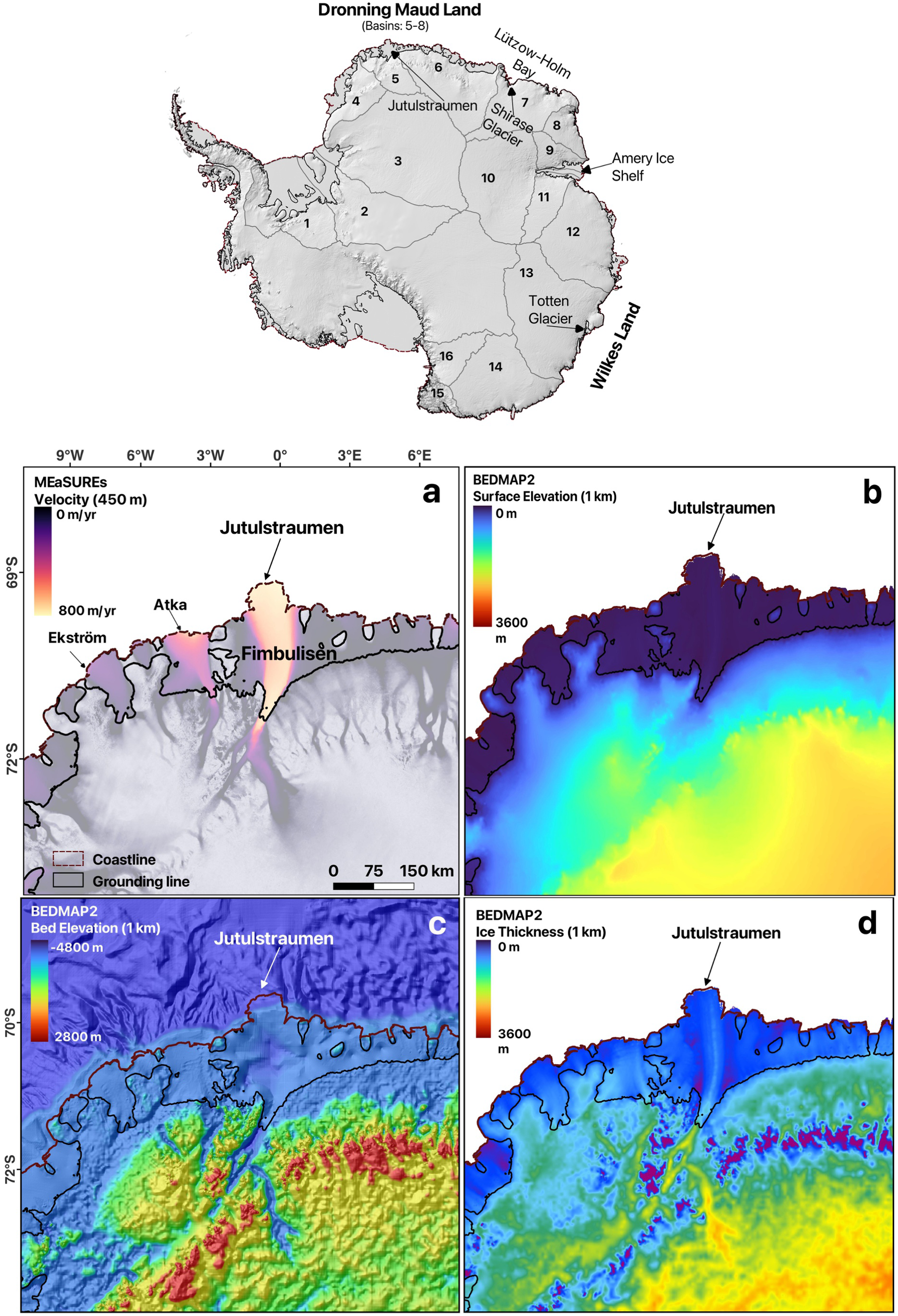
Figure 1. Regional glacial and topographic setting of Jutulstraumen in DML, with numbers referring todrainage basins in the EAIS. (a) MEaSUREs (Rignot and others, 2016) ice flow speed of the study area. (b) Surface elevation of the study area using Bedmap2, (c) Bed elevation of the study area using Bedmap2. (d) Ice thickness of the study area using Bedmap2. Bedmap2 is sourced from Fretwell and others (2013). The grounding line and coastline are from Rignot and others (2017). Note that gridspacing in panel ‘a’ is 400 m and in panels ‘b-d’ is 1 km.

Although DML has been gaining mass over recent decades, some studies indicate an increase in basal melt due to Warm Deep Water (WDW) influx (Lauber and others, 2023) and predict significant mass loss under future warming scenarios (Golledge and others, 2015, 2017; DeConto and others, 2021). Observations at Fimbulisen between December 2009 and January 2019 indicate an increase in the influx of WDW after 2016, resulting in an increase in basal melt rate of ∼0.62 m yr⁻¹ (Lauber and others, 2023). This change has been linked to decline in sea-ice concentrations and intensified subpolar westerlies in the region (Lauber and others, 2023). Furthermore, model predictions have suggested that the Recovery Basin in DML will be vulnerable to increasing ocean temperatures under a high emissions future warming scenario (Golledge and others, 2015, 2017). Indeed, some studies suggest substantial mass loss in the DML region by 2300 following a 3°C warming emission scenario (DeConto and others, 2021), albeit with high uncertainties. As such, continued increases in incursion of warm water events and projected future warming could further increase basal melt, thereby impacting the ice-shelf mass balance in DML earlier than anticipated. However, there exists a gap in systematic observations of glacier dynamics of major glaciers in this region. Without those observations it is challenging to understand the ongoing regional response to current and future climate change.

Our aim is to conduct the first long-term, systematic observations of Jutulstraumen, one of the largest outlet glaciers in DML, to improve our understanding of its recent dynamics from the 1960s to present (2022) and explore its future dynamics. This is undertaken using remotely sensed satellite imagery and several secondary datasets to analyze changes in glacier dynamics based on (1) ice front positions; (2) ice velocity (Gardner and others, 2019; ENVEO and others, 2021); (3) surface elevation change (SEC) (Schröder and others, 2019; Smith and others, 2020; Nilsson and others, 2022); (4) GL position (Haran and others, 2005, 2014; Bindschadler and Choi, 2011; Rignot and others, 2016); and (5) structural mapping (Fricker and others, 2005; Holt and others, 2013; Walker and others, 2015).

2. Study area and previous work on Jutulstraumen

The Fimbulisen is the largest ice shelf in the EAIS (∼39 400 km²) located between 71.5° S–69.5° S and 3° W–7.5° E. Jutulstraumen (‘The Giant’s Stream’ in Norwegian) is a fast-flowing ice stream (∼700 m yr⁻¹) that feeds the central part of the ice shelf (Figs. 1 and 2, Lunde, 1963; van Autenboer & Decleir, 1969; Gjessing, 1970) and has an annual ice discharge of 30 ± 2.2 Gt yr^-1 between 2009 and2017 (Rignot and others, 2019). The average mass balance of Jutulstraumen has been estimated at+33 Gt between 1979 and 2018 (Rignot and others, 2019). There has been only one major calvingevent recorded between the 1960s and 2022, occurring in 1967 (van Autenboer & Decleir, 1969; Vinje, 1975; Swithinbank and others, 1977; Kim and others, 2001) when a ~100 km long by ~50 km wideiceberg calved from Jutulstraumen’s floating ice tongue (named ‘Trolltunga’) along newly formedperpendicular rifts (Vinje, 1975; Humbert & Steinhage, 2011). This calved iceberg then drifted along theWeddell Sea for more than 13 years (Vinje, 1975).

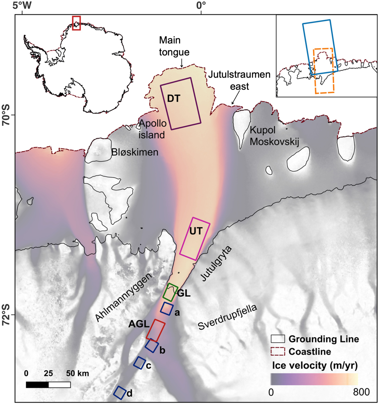
Figure 2. Location map of Jutulstraumen, EAIS overlain with MEaSUREs ice velocity. Grounding line(solid black) and coastline (dashed maroon) is from MEaSUREs (Rignot and others, 2017). Velocity analysis is undertaken in each of the four boxes in the map marked as down-ice tongue (DT), up-icetongue (UT), grounding line (GL) and above grounding line (AGL). Location of 20 x 20 km sampling boxes (navy blue) used to extract elevation change data from Schröder and others (2019), Smith and others (2020) and Nilsson and others (2022). Each sample box represents a specific distance from thegrounding line to understand the surface elevation change at (a) 20 km, (b) 60 km, (c) 80 km and (d)120 km from the grounding line. Note that the sample boxes used for elevation change are different from those used for ice velocity measurements because the velocity analyses primarily focus onchanges at and downstream of the grounding line, whereas the elevation change boxes were designed to capture major changes extending further upstream into the catchment area. ERA-5 2 m air temperaturedata were extracted from the dashed orange box, and Nimbus-7 sea ice concentration data were extracted from the solid light blue box (top right insert).

Jutulstraumen is pinned by ice rises on either side of the ice tongue (Kupol Moskovskij to the east and Bløskimen and Apollo Island to the west) (Figs. 1 and 2, Matsuoka and others, 2015), which may influence the flow and contribute to a stabilizing effect on the current ice-shelf configuration (Melvold and Rolstad, 2000; Goel and others, 2020). The main trunk of Jutulstraumen drains a major valley that ranges between 20 and 200 km wide and begins ∼60 km inland of the modern GL and cuts through a significant coastal mountain range: the massifs Sverdrupfjella to the east and Ahlmannryggen to the west (Fig. 1, Humbert and Steinhage, 2011). The valley through which Jutulstraumen flows is a graben resulting from major rifting following the breakup of Gondwana (Fig. 1c, Decleir and van Autenboer, 1982; Wolmarans and Kent, 1982; Melvold and Rolstad, 2000; Ferraccioli and others, 2005). The depth of the Jutulstraumen trough, estimated at ∼1500 m below sea level at the deepest part (Fig. 1, Gjessing, 1970; Decleir and van Autenboer, 1982; Melvold and Rolstad, 2000), allows the ice to drain from the EAIS interior and has the potential to make the area susceptible to ocean warming. However, recent modeling has explored the sensitivity of Jutulstraumen to mid-Pliocene warming (Mas e Braga and others, 2023), a period which is often used as an analogue for a near-future climate state (DeConto and others, 2021), and their findings highlight that the ice stream thickens by ∼700 m, despite its retrograde bed slope. This thickening was attributed to lateral stresses at the flux gate constricting ice drainage and thus stabilizing the GL (Mas e Braga and others, 2023).

Previous research suggests that recent (2010–2011) ocean conditions were relatively cold and dominated by Eastern Shelf Water in the cavity beneath the ice tongue (Hattermann and others, 2012), with an estimated mean basal melt rate of ∼1 m yr⁻¹ based on interferometric radar and GPS-derived strain rates in the central part of Fimbulisen (Langley and others, 2014). The basal melt rate has been shown to vary between 0.4 and 2.8 m yr⁻¹ based on the different methods used, such as oceanographic measurements (Nicholls and others, 2008; Hattermann and others, 2012), satellite altimetry and InSAR data (Shepherd and others, 2010; Pritchard and others, 2012; Depoorter and others, 2013; Rignot and others, 2013) and oceanographic modeling (Smedsrud and others, 2006; Timmermann and others, 2012). However, recent observations show pulses of WDW entering the cavity since ∼2016, occasionally reaching over −1.5°C, with peak temperatures up to 0.2°C, contributed to a basal melt rate of 0.62 m yr⁻¹ and which has been linked to mass loss of 15.5 Gt yr⁻¹ between 2016 and 2019 (Lauber and others, 2023). These changes, driven by a positive Southern Annular Mode (SAM) resulting in stronger westerlies and reduced sea ice, could significantly impact the ice shelf’s mass balance and its buttressing effect on inland ice.

In summary, the response of EAIS to climate change is complex and varies across different regions. This is influenced by factors such as presence or absence of warm ocean conditions and bed topography (Morlighem and others, 2020). The lack of observational data for several major outlet glaciers, including Jutulstraumen, makes it even more challenging to understand how the glaciers in the EAIS are currently responding, or will respond to, changing climate. Thus, in this paper, we conduct systematic observations of Jutulstraumen between the 1960s and 2022 with the aim of improving our understanding of the changing ice conditions in this part of DML.

3. Data and methods

3.1. Ice front position change

In this study, a combination of satellite images from Landsat 1MSS (1973–74), Landsat TM 4 and 5 (1989–91), Landsat 7 ETM+ (1999–2013) and Landsat 8 OLI/TIRS (2013–2022) with cloud-free conditions were acquired from the USGS Earth Explorer website (https://earthexplorer.usgs.gov) to map changes in Jutulstraumen between 1963 and 2022 (Table S1). In addition, we use an orthorectified declassified ARGON satellite photograph of 1963 (Kim and others, 2001). A time series of ice front position change was generated between 1963 and 2022 based on the availability of imagery during the austral summer in the broadest sense (October–April). The annual ice front positions were manually digitized using ArcGIS Pro 2.8.2. The changes in position were quantified using the well-established box method which accounts for any uneven changes along the ice front (Moon and Joughin, 2008). Given the shape and orientation of Jutulstraumen’s main ice tongue (Fig. 4), a curvilinear box was used (Lea and others, 2014). It should be noted that, in addition to the main outlet of Jutulstraumen, there exists an ice front along the eastern margin, separated by a rift, referred to as Jutulstraumen east hereafter (Figs. 2, 4c and d). The curvilinear box method was applied separately here. The errors in our measurements arise from co-registration of the satellite images (Landsat 1–8) with a 2022 Landsat-8 base image (which is quantified as the offset between stable features in image pairs, generally estimated at 1 pixel) and the manual digitization of the ice front estimated at 0.5 pixels (Miles and others, 2013, 2016, 2018, 2021; Black and Joughin, 2022). The error was quantified using error propagation, considering the varying spatial resolutions of the imagery and the temporal gaps between them. The estimated error ranges from ±3 to ±63 m yr⁻¹ (Table S1).

3.2. Glacier velocity

Average annual velocities were acquired from the Inter-mission Time Series of Land Ice Velocity and Elevation (ITS_LIVE) annual velocity mosaics (Gardner and others, 2019, 2018) between 2000 and 2018. These velocity mosaics were derived from a combination of Landsat-4, -5, -7 and -8 with the use of auto-RIFT feature tracking with each velocity mosaic having a spatial resolution of 240 m (Gardner and others, 2019). In addition, ENVEO (ENVEO and others, 2021) velocity mosaics were also used to extract velocity between 2019 and 2021. The ENVEO velocity mosaics were derived from repeat-pass Sentinel-1 Synthetic Aperture Radar (SAR) datasets using feature-tracking and are provided monthly between 2019 and 2021 at spatial resolution of 200 m. The monthly ENVEO velocity mosaics were averaged over 12-months for each year between 2019 and 2021 to compare with the ITS_LIVE annual velocity mosaics.

Velocities were extracted from the four regions shown in Fig. 2. Following Miles and others (2018) and Picton and others (2023), we calculated the mean annual velocities by averaging all available data within each sampling box, provided that data coverage of more than 20% was observed. However, a scarcity of data resulted in limited coverage, especially prior to 2000 (Table S2). Error estimates were provided for both datasets (Gardner and others, 2019, 2018; ENVEO and others, 2021), with each pixel having its own error term. The annual error values were then calculated by applying the error propagation formula to the individual error values (grid cells) within each sample box for each ITS_LIVE annual velocity error mosaics (Gardner and others, 2019, 2018). Similarly, using error propagation, the monthly errors were calculated for the ENVEO velocity error mosaics. Subsequently, the annual velocity errors for 2019–2021 were computed using error propagation, accounting for the uncertainties in the monthly errors (ENVEO and others, 2021). Some of the velocity measurements were omitted from the analysis given the mean error from each sample box was more than 50% of the mean velocity magnitude (Miles and others, 2018; Picton and others, 2023) (Table S2). The accompanying errors associated with the velocity mosaics at DT, UT, GL and AGL ranged from ±0.5 to ±163 m yr⁻¹.

3.3. Elevation change

A range of previously published elevation change datasets were compared to understand any changes along Jutulstraumen. The elevation change measurements were extracted at four locations at 20, 60, 80 and 120 km inland of the GL (Fig. 2). The average monthly elevation change was calculated by averaging all available data within each 20 × 20 km sample boxes (Fig. 2) using datasets provided by Schröder and others (2019), Smith and others (2020) and Nilsson and others (2022). We use the accompanying uncertainty estimates provided with the three datasets and calculated the monthly error by applying the error propagation formula to the individual error values (grid cells) within each sample box.

The dataset provided by Schröder and others (2019) is a combination of multiple satellite missions (e.g. ERS-1/2, Geosat, Seasat, Envisat, ICESat and CrysoSat-2) between 1978 and 2017, but referenced to September 2010. The dataset is provided with a horizontal resolution of 10 km and the associated monthly uncertainties at the sampling boxes range from ±0.1 to ±10 m yr⁻¹ (Schröder and others, 2019).

Nilsson and others (2022) provided a monthly elevation change dataset that spans from 1985 to 2020, with reference to December 2013. This dataset was produced as a part of the NASA MEaSUREs ITS_LIVE project. It also combines measurements from several satellite missions (e.g. ERS-1/2, Geosat, Seasat, Envisat, CrysoSat-2, ICESat and ICESat-2) at a horizontal resolution of 1920 m. Monthly mean SEC was extracted from the same sampling boxes. The accompanying monthly uncertainties at the sample locations range from ±0.05 to ±3 m yr⁻¹. To allow a more direct comparison between the datasets, the SEC measurements from Schröder and others (2019) were recalculated relative to December 2013, aligning with the reference year used in Nilsson and others (2022). The two datasets were analyzed from April 1992, as it is the earliest common data availability month at all four sample locations. We then calculate the 5 year moving averages for the two datasets. The errors associated with the 5 year moving average were determined from monthly errors using error propagation.

Additionally, the dataset provided by Smith and others (2020) is derived from ICESat and ICESat-2 missions, spanning from 2003 to 2019, with horizontal resolution of 5 km (Smith and others, 2020). The associated uncertainties range between ±0.001 and ±0.006 m yr⁻¹. To compare the three datasets, the mean rates of elevation change in each box were calculated for Schröder and others (2019) from 2003 to 2017, Smith and others (2020) from 2003 to 2019 and Nilsson and others (2022) from 2003 to 2020 (Table S3).

3.4. GL changes

We analyze five previously published GL datasets spanning various dates between 1992 and 2018, along with new GL positions mapped in this study using manual digitization between 1990 and 2022 (Fricker and others, 2009; Christie and others, 2016). Together, all these datasets were derived through either manual delineation or Differential Interferometric Synthetic Aperture Radar (DInSAR) techniques. It should be noted that each dataset identifies distinct features within the grounding zone, which makes comparison of changes through time more challenging (Fig. 7a, Fricker and others, 2009; Brunt and others, 2010). For example, the Making Earth Science Data Records for Use in Research Environments (MEaSUREs) GL dataset (Rignot and others, 2016) detects the landward limit of tidal flexure (F), Antarctic Surface Accumulation and Ice Discharge (ASAID) dataset (Bindschadler and Choi, 2011) detects the break-in slope, I_b, whereas this study detects the local elevation minimum, I_m.

In this study, we manually delineate the grounding line positions using Landsat 4–8 images, during austral summers (October to April) between 1990 and 2022, following the methods outlined in Fricker and others (2009) and Christie and others (2016). As optical satellite imagery cannot precisely determine the ‘true’ GL (G), the break-in-slope (I_b) or the local elevation minimum (I_m) (Fig. 7a) is generally used as a proxy for G. Here, we identify I_m as a shadow-like change in the brightness of the imagery (Fricker and Padman, 2006; Fricker and others, 2009; Bindschadler and Choi, 2011; Christie and others, 2016; Christie and others, 2018) and digitized it on the georeferenced cloud-free Landsat images. To determine whether the mapped GL advanced or retreated, we used the box method (Moon and Joughin, 2008), with the box extending to the ends of the mapped GLs. We used this method because it provides an average GL position change across the glacier. We also estimated a positional uncertainty of ∼±100 m, following Bindschadler and others (2011) and Christie and others (2016).

In addition, among the manually delineated GL datasets is the ASAID dataset, which was created using a combination of photoclinometry applied to satellite imagery (primarily Landsat 7 ETM+), elevation profiles from ICESat data and visual analysis of optical satellite imagery. The GL was digitized on Landsat 7 ETM+ images between 1999 and 2003 by identifying changes in image brightness indicative of the break-in-slope (I_b). The average estimated positional uncertainty associated with the ASAID GL position for outlet glaciers is ±502 m (Bindschadler and Choi, 2011). Similarly, The Mosaic of Antarctica (MOA) GL dataset was derived by manually delineating the most seaward break-in slope (I_b) on highly contrast-enhanced MOA surface morphology images (Scambos and others, 2007) for 2004 and 2009, with an associated uncertainty of ±250 m (Haran and others, 2005, 2014). Furthermore, some GL positions are also derived using DInSAR. The MEaSUREs dataset provides GL positions between 1992 and 2014, identifying the landward limit of tidal flexure (F). This dataset was derived using DInSAR from Earth Remote-Sensing Satellites 1 and 2 (ERS-1 and ERS-2), RADARSAT-1, RADARSAT-2, the Advanced Land Observing System Phased Array type L-band Synthetic Aperture Radar (ALOS PALSAR), Cosmo Skymed and Copernicus Sentinel-1 (Rignot and others, 2016). The associated uncertainty with the dataset is estimated at ±100 m (Rignot and others, 2016). The European Space Agency’s Antarctic Ice Sheet Climate Change Initiative (AIS CCI) has also been derived using DInSAR from ERS-1, ERS-2 and Sentinel-1 imagery collected between 1996 and 2020, with an estimated error of ±200 m. In this dataset, the upper limit of vertical tidal motion has been used as an approximation of flexure point (F) in the grounding zone. The Mohajerani and others (2021) dataset employs a fully convolutional neural network to automatically delineate GLs for 2018 by identifying the landward limit of tidal flexure (F) using DInSAR data, with associated uncertainty of ±232 m.

3.5. Structural glaciological mapping

To understand the structural glaciology of Jutulstraumen, some of the major surface structural features were manually mapped on selected cloud-free optical satellite imagery in 1986, 2001, 2015 and 2022 using bands with highest spatial resolution, e.g. band 4 in Landsat 1-4 and band 8 for Landsat 7 ETM+ and Landsat 8 OLI/TIRS (Holt and others, 2013; Table S1). The major structural features included rifts, fractures, crevasses, longitudinal flow features (flowstripes, flow bands, streaklines), surface expressions of major basal channels, ice rises and ice rumples. The criteria used to identify these various features is same as the approach taken by Glasser and others (2009) and Holt and others (2013) (Table 1), except for the identification of basal channels which has been adapted from Alley and others (2016).

Table 1. Ice-shelf features, examples, identifying criteria and significance adapted from Glasser and Scambos (2008), Glasser and others (2009), Humbert and Steinhage (2011) and Holt and others (2013)

To measure in more detail the rifts that propagate from the ice front into the ice tongue in more detail (Fig. 3), a total of 200 cloud-free images were selected. These images were collected during the austral summers between 2003 and 2022. They were obtained from the Moderate Resolution Imaging Spectroradiometer (MODIS) and have a spatial resolution of 250 m. For the purposes of this study, the austral summer is considered between October and early April (cf. Walker and others, 2015). Following the methodology in Fricker and others (2005), we measured the rift length from a consistent point at the ocean-end of the rift to the ‘rift tip’ (Fig. 3). The ‘rift tip’ was identified as the first point on the glacier where the rift pixel is discernible, i.e. the point in the image where rift occupied enough of the pixel to provide a good contrast against the background (Fricker and others, 2005; Walker and others, 2015; Holt and Glasser, 2022). Since these rifts are located at the ice front, it is possible that the ocean-end of the rifts may undergo discrete minor calving events between subsequent images, potentially leading to rift shortening. In such cases, when calving leads to rift shortening, the rift is assigned a new name to reflect the updated starting point. For example, RW3 becomes RW6, after the calving event in 2011 (Fig. 9a). This results in a consistent start point for the rifts across all subsequent images, enabling accurate measurement of rift propagation into the ice tongue. In addition, we determined the average annual and austral summer propagation rates by applying a linear fit to the time series data of rift lengths utilizing the least squares method, following methodology outlined in Walker and others (2015). The linear regression analysis was performed to estimate slopes for each summer season for each rift (Case A, Tables S4 and S5). Case B represents the linear fit applied to the differences in rift lengths between the end of one summer and the start of the next summer. Case C denotes a linear fit applied to the entire dataset of rift lengths for each rift (Tables S4 and S5).

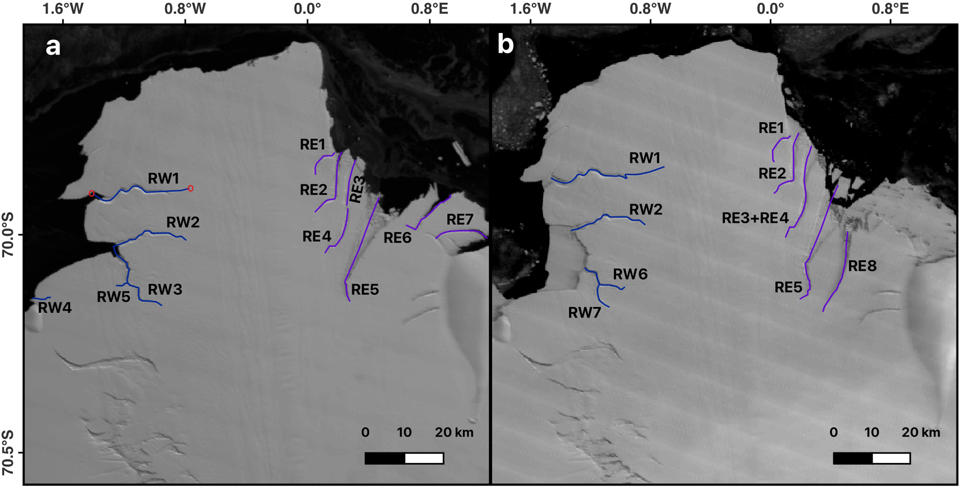
Figure 3. (a–b) Rifting of the ice-shelf front monitored in this study (blue lines: western rifts (RW) and purple lines: eastern rifts (RE)) with background image: (a) MODIS images acquired on 13March 2006 and (b) acquired on 16 December 2016. (b) shows the rifts formed later in the study period (RW6, RW7, RE8). It also shows that rift RE3 lengthened and joined RE4 (later named RE3 + RE4). Note: Red circles in (a) denote start and end points for RW1, a front-initiated rift.

3.6. Relationship between rift propagation and environmental variables

To determine whether a relationship between rift propagation and environmental variables exists in Jutulstraumen (Bassis and others, 2008; Walker and others, 2013, 2015), we compare the rift propagation with (a) air temperature and (b) sea-ice concentrations for the period of October to early-April (Figs. 2 and 3) between 2003 and 2022.

1. Air temperature

Daily mean near-surface (2 m) air temperature data were extracted for all austral summers between 2003 and 2022, which is provided at a 0.25° (30 km) from ERA5 reanalysis data (Hersbach and others, 2023). To understand the link between rift propagation and temperature, we calculated the positive degree-days (PDDs) using mean degree-hour method (Day, 2006). PDD is defined as the total sum of hourly averaged temperatures per day above 0°C. The PDDs were summed over each season, and we analyzed whether there was a significant correlation between PDD and rift propagation rate.

2. Sea-ice concentration

Sea-ice concentration data were extracted from Nimbus-7 SMMR and DMSP SSM/I-SSMIS Passive Microwave Data V002 (DiGirolamo and others, 2022). This region includes multi-year sea ice and mélange that fills the rift openings. The spatial resolution of the sea-ice concentration dataset is 25 km. As both sea-ice concentration and rift lengths have strong seasonal signals, a linear regression was performed to understand if changes in sea-ice concentration influences the propagation rate (Walker and others, 2015). To directly compare the variability in sea-ice concentration with rift propagation rates, the seasonal component of sea-ice concentration was first removed.

4. Results

4.1. Ice front position

Our earliest images date from 1963 and 1973 and confirm that a large calving event occurred between these dates, resulting in ∼60 km of retreat (Fig. 4). Our analyses indicate that the ice front gradually advanced between 1973 and 2022 and that it is currently ∼30 km landward from its near maximum extent prior to the calving event in 1967. Furthermore, there is little evidence that the shape of the ice front has exhibited any major change between 1973 and 2022 (Fig. 4), suggesting no major calving events have taken place over this period. In addition, the ice front advance rate showed limited changes with an average of ∼740 m yr⁻¹ between 1985 and 2022, albeit with small interannual variations in the ice front advance rate (Fig. S1).

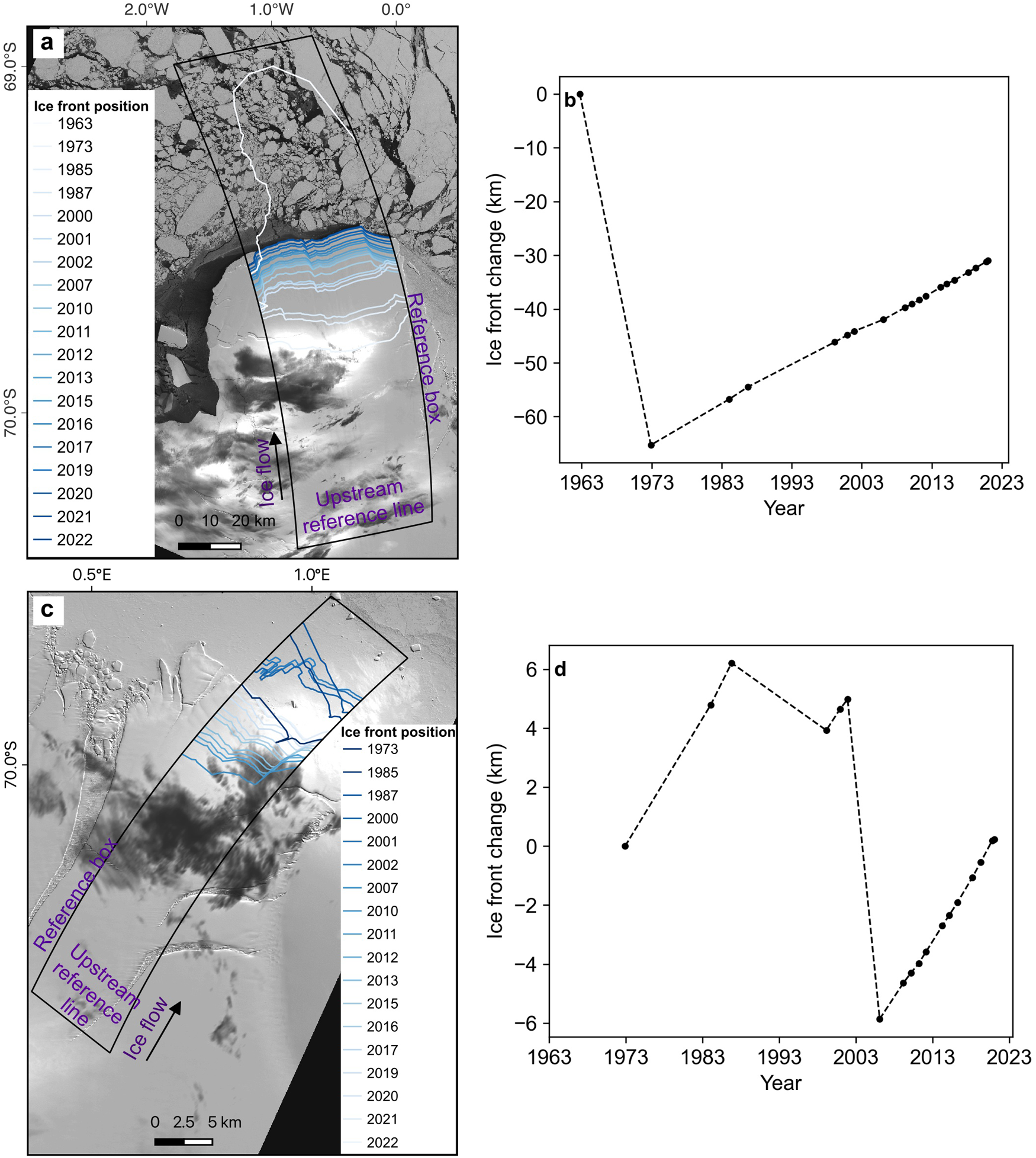
Figure 4. (a) Mapped ice front position of the main tongue of Jutulstraumen between 1963 and 2022. (b)Ice front position change of Jutulstraumen’s main tongue during 1963–2022 from the black curvilinearbox delineated in (a). (c) Mapped ice front position of the eastern extension of Jutulstraumen between1973 and 2022. (d) Ice front position change of eastern extension of Jutulstraumen during 1963–2022from the black curvilinear box delineated in (c). The background image in (a) and (c) is a Landsat- 8image from 13 October 2021. Note that the errors are too small to be visible at this scale but see TableS1.

At the smaller Jutulstraumen east outlet, the ice front retreated by ∼2.3 km between 1987 and 2000, followed by a slight advance of ∼1 km between 2000 and 2002, a large retreat of ∼ 10 km between 2002 and 2007, and with a further re-advance of ∼6 km between 2007 and 2022 (Figs. 4c and d).

4.2. Glacier velocity

The glacier velocity trend along the floating ice tongue showed little overall change between 2000 and 2021, with only minor interannual fluctuations (Fig. 5). As a result, the mean annual velocity was estimated at ∼720 ± 66 m yr⁻¹ across all sampling boxes over the floating ice tongue. This estimated glacier velocity is consistent with the mean rate of advance described in the previous section, which we calculate as ∼740 m yr⁻¹, albeit with some minor fluctuations between 1985 and 2022 (Figs. 5 and S1). The mean velocity is in the same range at DT, UT and GL, but is much less at box AGL ( Figs. 2 and 5). The associated uncertainties ranged from ±0.5 to ±163 m yr⁻¹ (Fig. 5). Although we observed a 10% increase in velocity at UT between 2011 and 2012, the absolute value of increase (55 m yr⁻¹) is smaller than the associated error (±118 m yr⁻¹). In addition, the 15% decrease in velocity at AGL between 2008 and 2009, with an absolute velocity decrease of 61 m yr⁻¹ is smaller than the associated error of ± 62 m yr⁻¹.

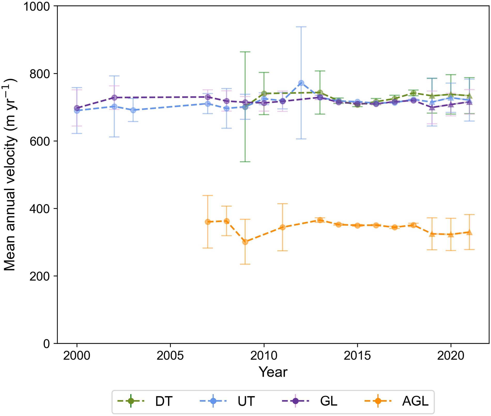
Figure 5. Trends of mean annual velocity extracted from Jutulstraumen at the four locations at down-icetongue (DT), up-ice tongue (UT), grounding line (GL) and above the grounding line (AGL) (see Fig. 2for location). Velocity is extracted from ITS_LIVE (circle) and ENVEO (triangle) velocity mosaicsbetween 2000 and 2021 (Gardner and others, 2019; ENVEO and others, 2021).

4.3. Elevation change

Our results indicate that elevation change trends obtained from Schröder and others (2019) and Nilsson and others (2022) are less comparable and associated with higher uncertainties pre-2003, with notably inconsistent trends between 1992 and 2003 at all sample locations (20, 60, 80, and 120 km inland of GL). However, a general agreement between the two datasets is observed after 2003, with a clear thickening trend of the grounded ice observed from ∼2003. It is also worth noting that both datasets manifest some interannual variability (Fig. 6). Nonetheless, we observed an overall thickening when averaged across all sampling boxes, at a rate of +0.11 ± 0.1 m yr⁻¹ between 2003 and 2017 (Schröder and others, 2019) and +0.14 ± 0.04 m yr⁻¹ between 2003 and 2020 (Nilsson and others, 2022) upstream of the GL. Furthermore, a similar pattern of thickening of the grounded ice is also observed in the dataset provided by Smith and others (2020) with an average rate of +0.17 ± 0.005 m yr⁻¹ (Table S3).

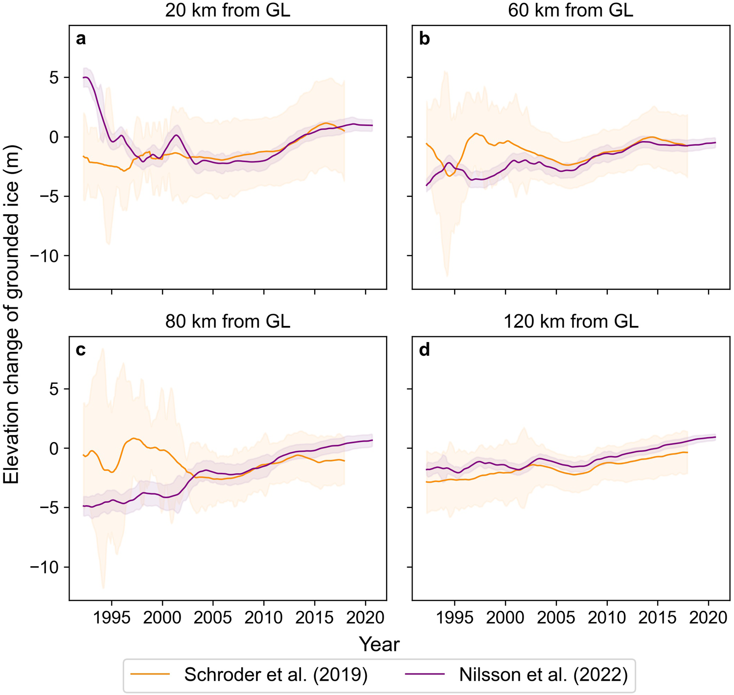
Figure 6. Monthly elevation changes of the grounded ice observed at four locations, i.e. (a) 20 km, (b) 60 km, (c) 80 km and (d) 120 km inland from the grounding line (GL) at Jutulstraumen between 1992 and 2020, obtained from Schröder and others (2019) and Nilsson and others (2022). The solid lines represent 5 year moving averages, and the shaded area represents the corresponding error propagation.

4.4. Grounding line changes

In this section, we present a comprehensive compilation of all available GL positions, categorized according to the two primary methodologies of determining GL position detailed in Section 3.4. Figure 7b shows the GL positions acquired using DInSAR. Notably, the DInSAR-derived data for Jutulstraumen in 1994 are provided by both MEaSUREs (4/3/1994) and AIS CCI (derived from double differences of three subsequent images: (4/3/1994, 7/3/1994, 10/3/1994) coinciding on the same date. The GL positions from these two datasets for 1994 align closely.

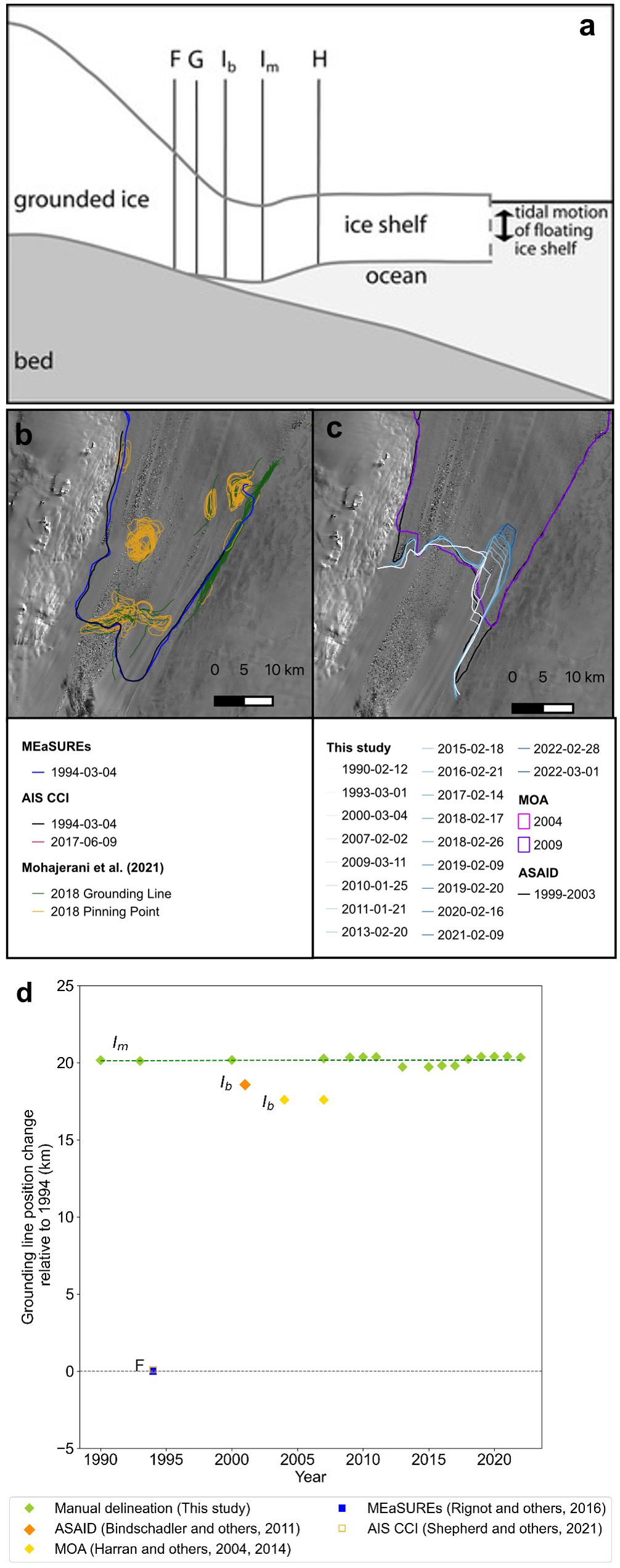
Figure 7. Grounding line (GL) position change of Jutulstraumen based on different GL datasets. (a) Schematic illustration of grounding zone features from Fricker and others (2002) (b) GL position based on vertical motion at the floating part using DInSAR data (MEaSUREs, AIS CCI and Mohajerani and others, 2021). (c) GL position based on manual delineation of break-in slope (ASAID, MOA, this study). (d) Change in GL position relative to observed 1994 position from all datasets.

More recently, the dataset provided by Mohajerani and others (2021), which also used DInSAR data as input for a fully convolutional neural network, includes clusters of GL positions (green) and pinning points (yellow) for 2018. Note that within the cluster that is furthest upstream, there are some GL positions that correspond to the flexure location or the hinge line, F (Fricker and Padman, 2006; Fricker and others, 2009; Friedl and others, 2020) and these align closely with the 1994 GL positions provided by MEaSUREs (Rignot and others, 2016) and the AIS CCI (Fig. 7). This overlap at the flexure location suggests a consistency between the three datasets. Meanwhile, other GL positions within this cluster are associated with localized features of the grounding zone such as pinning points (Fig. 7b). Overall, this suggests limited or no change in GL position over the 24 year period between 1994 and 2018.

Figure 7c shows the GL position determined by previously published manual delineations of the break-in slope, I_b (ASAID and MOA) and of the assumed local elevation minimum, I_m, mapped in this study. The ASAID and MOA GL positions were digitized at similar locations, showing limited change over time. However, the GL positions obtained in this study exhibits a slow advance of ∼200 m (∼6 m yr⁻¹ on average) between 1990 and 2022 (Fig. 7d).

Figure 7d compares the manually delineated GL positions (ASAID, MOA, this study) with the earliest available GL positions derived from DInSAR (MEaSUREs). It is evident from Fig. 7d that the GL positions obtained from MEaSUREs and AIS CCI which identifies the landward limit of the ice flexure caused by tidal movement (F), are consistently located much further up the ice tongue compared to those obtained from manual delineation of break-in slope, I_b (ASAID, MOA) and the local elevation minimum, I_m (this study). For example, the 1994 DInSAR-derived GL position is ∼18 km upstream from the 1993 GL position (I_m) identified in this study. Similarly, the furthest upstream GL position from the 2018 DInSAR-derived cluster provided by Mohajerani and others (2021) is ∼16 km upstream of the 2018 GL position identified in this study. This clearly emphasizes that GL positions acquired using different methods are not directly comparable as they are recording different features of the grounding zone (Fricker and Padman, 2006; Fricker and others, 2009; Friedl and others, 2020; Picton and others, 2023). However, taken together, there is little evidence for a major change in GL position at Jutulstraumen (Fig. 7c), although our manually digitized method suggests there may have been a very small (∼200 m) advance, with approximately ±100 m uncertainty associated with it (see white to blue lines in Fig. 7b).

4.5. Structural glaciology

The features on Jutulstraumen ice tongue, based on the criteria in Table 1, are displayed in Fig. 8. The western side of the ice tongue has previously been observed to be heavily rifted (cf. Humbert and Steinhage, 2011). Several distinct rifts filled with sea ice/mélange have lengthened during the observation period, predominantly on the western side, with additional rifts forming and expanding on the eastern side near Jutulgryta (Figs. 2 and 8). The western side also shows a consistent area of fracture traces, with a slight increase in these features noted over the study period (Fig. 8). Moreover, a surface crevasse field is located near Ahlmannryggen on the western side, with a smaller crevasse field on the eastern side near Jutulgryta (Figs. 2 and 8, Humbert and Steinhage, 2011). A mélange zone has been observed between the western crevassed field and Ahlmannryggen. Additionally, during our observation period (1986–2022), rifts at the ice front have continued to propagate, leading to small calving events on both the western and eastern margins of the ice tongue (Fig. 9).

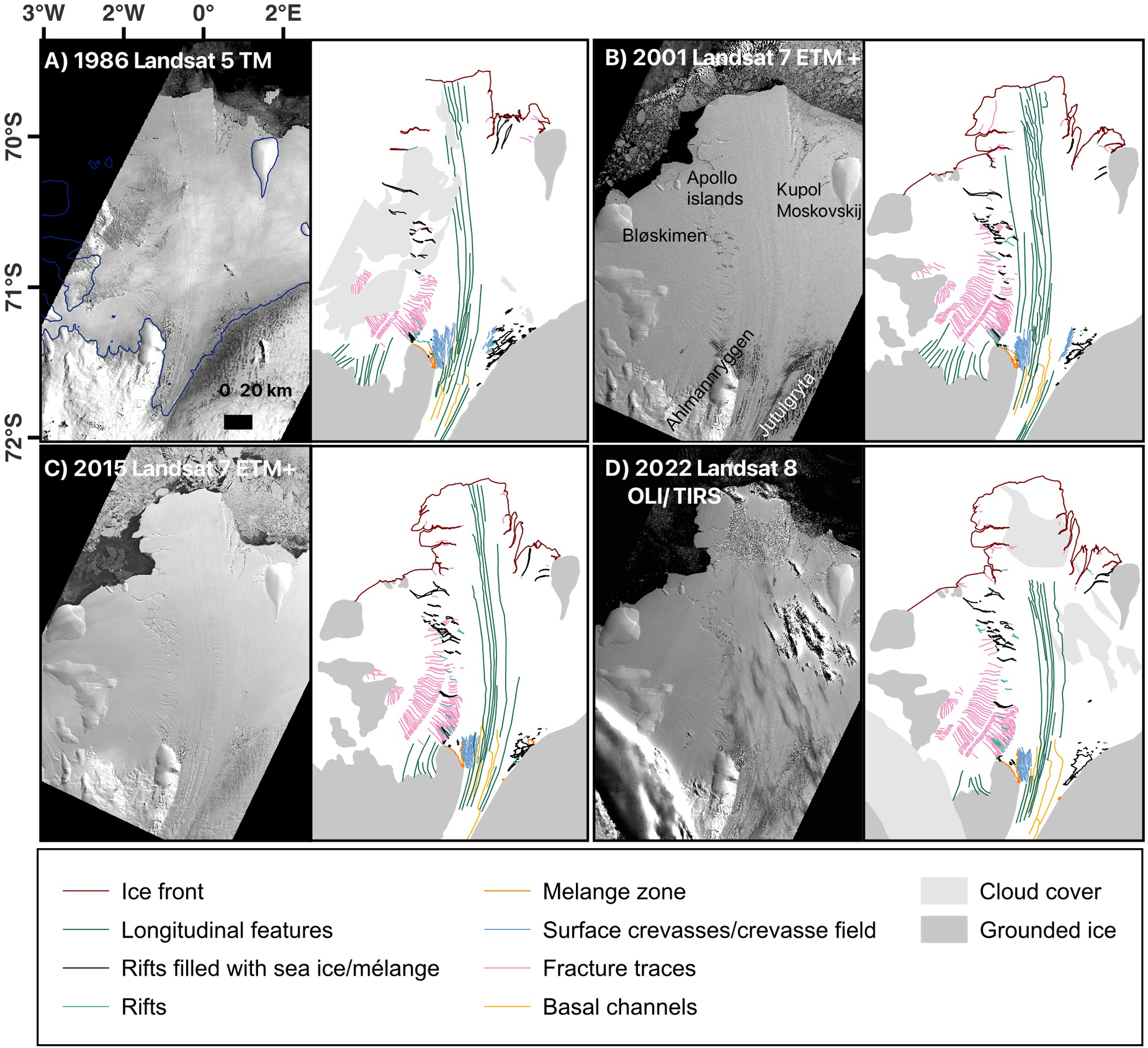
Figure 8. Structural evolution of Jutulstraumen illustrating widespread rifting from 1986 to 2020. Increased rifting is apparent on the western side of the glacier. The dark blue line in the 1986 satellite image is the MEaSUREs grounding line v2 (Rignot and others, 2017).

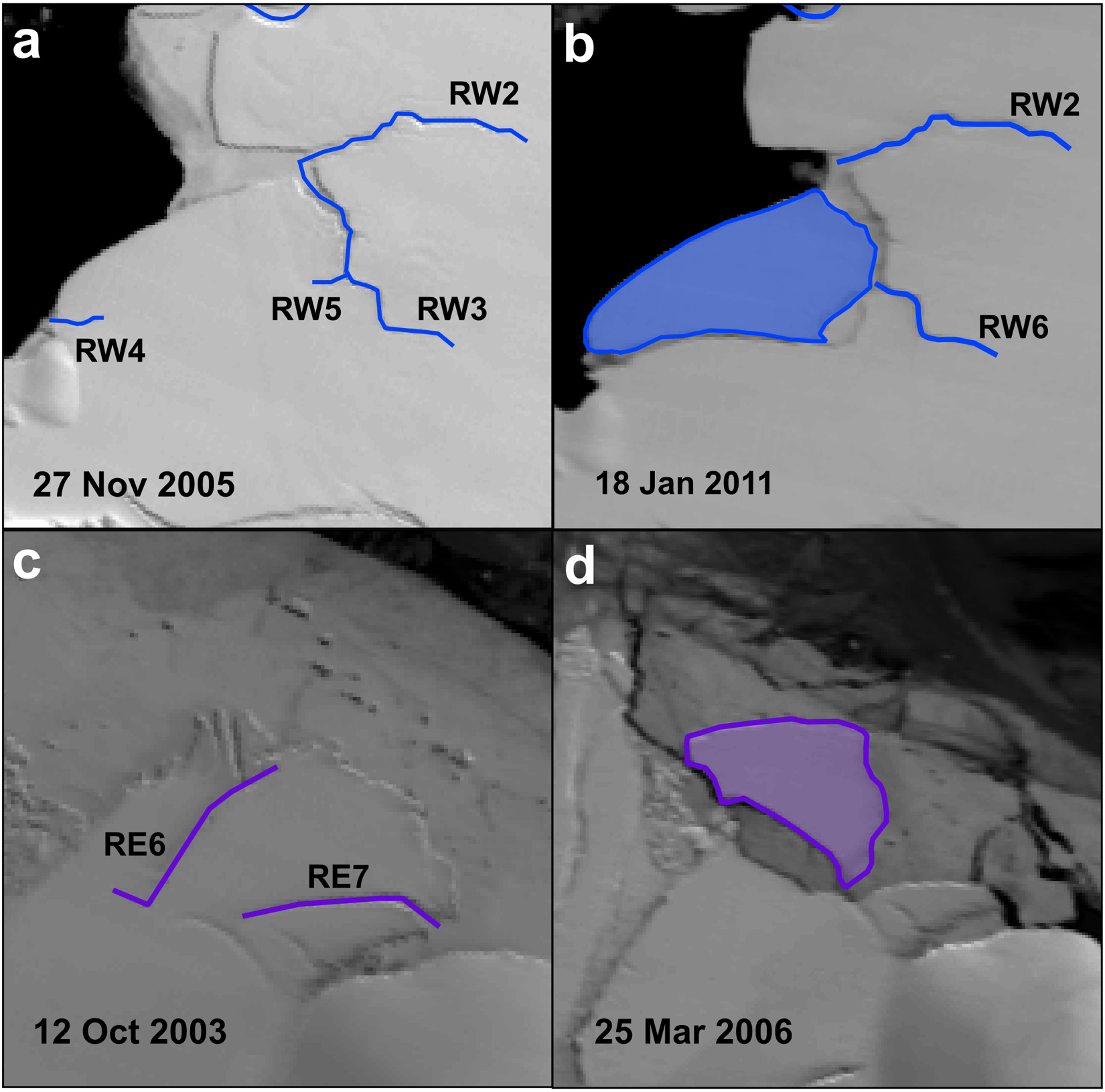
Figure 9. (a) Shows the calving of a small part on the eastern margin of Jutulstraumen between 27 November 2005 and 18 Oct 2011 due to propagation of rifts RW4 and RW5. (b) Shows the calving of a small part on the western margin of Jutulstraumen between 12 October 2003 and 25 March 2006 due to propagation of rifts RE6 and RE7.

While we do not attempt to quantify changes in all the features identified here (Fig. 8), we recognize and quantify 15 of the largest rifts propagating into the ice stream from the ice front which may later play an important role in future calving events.

4.5.1. Rift propagation and links to environmental variables

We examine seven major rifts on the western and eight on the eastern margin of Jutulstraumen (Fig. 3) using satellite imagery (MODIS) from 2003 to 2022. Note that these rifts appear to be a consequence of the ice shelf interaction with the topography near the ice front. For example, the rifts on the west appear to be related to re-activation of pre-existing fractures as the ice pulls away from the headland. On the eastern margin, however, the rifts appear to be associated with the ice shelf’s detachment from the ice rise (Kupol Moskovskij) at the front of the glacier. Overall, during the study period, most of these rifts lengthened during the austral summer and there was minimal change during the austral winter. Furthermore, in some seasons, the rift length at the beginning of austral summer was lower than the end of previous summer. This could be due to rift ‘healing’, snow accumulation at the rift tip, or the presence of sea ice/mélange in the rift cavity resulting in a lower estimation of rift length. Nevertheless, the 19 year time series compiled from MODIS imagery shows an overall increase in the lengths of all the rifts measured at different propagation rates (Tables S4, S5 and Fig. 10). Figure 10 shows seasonal variation in rift propagation superimposed on a multi-year linear trend.

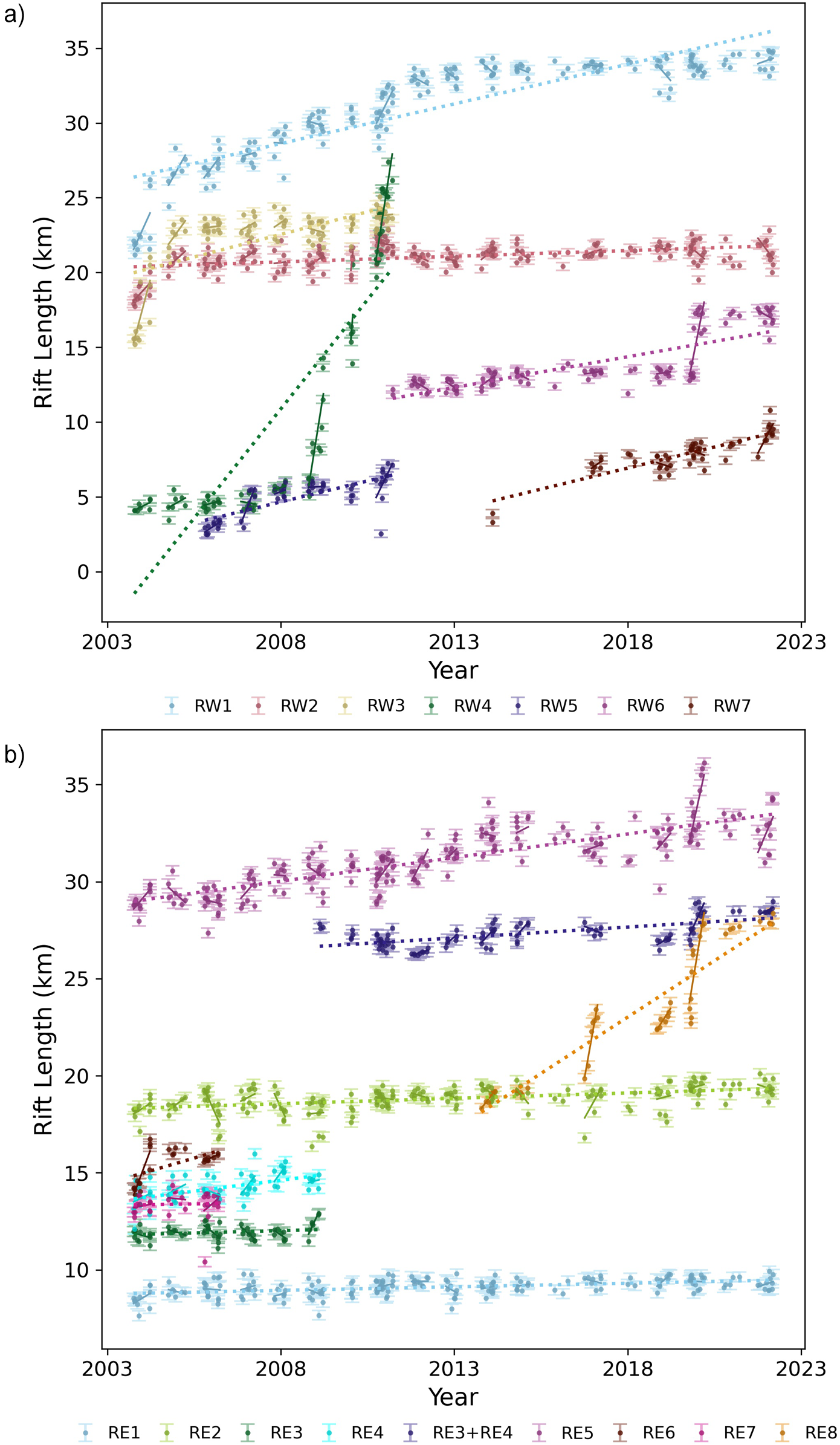
Figure 10. Measured rift lengths derived from MODIS imagery between 2003 and 2022 on the (a) westernside and (b) eastern side of Jutulstraumen. The error bars represent 1 pixel, where pixel size for MODISis 250 m. MODIS times series for RW1 to RW7 and RE1 to RE8 with linear regression analysis. Solidlines show the linear regression performed to estimate slopes for each summer season for each rift(Case A, Table S4, S5). Dashed lines denote a linear fit applied to the entire dataset of rift lengths foreach rift (Case C. Table S4, S5) (see Section 3.5).

All seven rifts monitored at the western side of Jutulstraumen exhibited increases in length, with periods of short-term decrease, at an overall long-term average rate of ∼2.4 m d⁻¹ from 2003 to 2022. In comparison, rifts on the eastern margin propagated at a slightly slower rate of ∼0.7 m d⁻¹. As they lengthened on the eastern margin, rift widening was also observed. For example, rift RE5, which formed ∼1986, widened by ∼3 km between 2003 and 2022 (∼0.4 m d^–1) and consequently opened-up toward the ocean and filled with sea ice/mélange (Fig. 3a). On the western margin, RW4 had the fastest long-term propagation rate (∼8 m d⁻¹) while RW2 had the slowest rate (∼0.2 m d⁻¹; Fig. 10, Table S4). On the eastern margin, RE8 had the fastest long-term rate (∼3.2 m d⁻¹), while RE1, RE2 and RE7 had the slowest rate (∼0.1 m d⁻¹; Fig. 10, Table S5). The highest propagation rates have been documented in those rifts that are relatively short-lived.

We find that most rift propagation rates tend to slow with time. For instance, the rates during 2003–11 were higher than those between 2012 and 2022, specifically for RW1 (2003–11: 3.1 m d⁻¹ and 2012–22: 0.3 m d⁻¹) and RW2 (2003–11: 0.9 m d⁻¹ and 2012–2022: 0.1 m d⁻¹). In addition, smaller rifts exhibited higher propagation rates. On the western margin, RW4 and RW5 showed propagation rates of approximately 8 and 1.6 m d⁻¹, respectively, until the calving event in 2011 (Table S4), when a small part (∼183 km²) of the ice front calved off (Fig. 9a). Similarly, the rifts RE6 and RE7 propagated at ∼1.4 and ∼0.1 m d⁻¹ from 2003 until a calving event in 2006 (Table S5), when a small part (∼128 km²) of the ice front calved off (Fig. 9b).

Note that, on the western margin, RW3 (yellow) was observed until 2011 when a small part calved off and the remaining fragment of RW3 was renamed as RW6 (violet) (Fig. 10a). On the eastern margin, RE3 (green) and RE4 (light pink), which were separate until 2009, merged in the latter half of 2009 and were renamed as RE3 + RE4 (brown) (Fig. 10b).

The patterns of rift propagation have been observed to be highly variable, ranging from 0 to 100 m d⁻¹, within each austral summer season (Fig. 10). The regression analysis determined that the propagation rates for each summer season were significantly different from each other between 2003 and 2022 at 95% confidence interval (Tables S4 and S5). In addition, the differences between rift length at the end and beginning of austral summer were mostly less than one pixel (<250 m), with instances of rift healing also observed, indicating minimal rift propagation during winter period (Walker and others, 2015). For Case C, the linear fit applied to the entire dataset showed variable rift propagation rates, as detailed in Tables S4 and S5. This analysis underlines the complex and variable nature of rift propagation rates.

Further analysis of factors that influence rift propagation rates reveals that the relationship between these rates and environmental conditions has no significant correlation (see Figs S3–S6). The 2 m air temperature observed over the sample box, covering the fast-flowing part of the glacier (Fig. 2), varied during austral summer (October–early April), ranging from −35°C to 4°C. Air temperatures typically peaked soon after late December and the PDDs typically occurred between December and February (Fig. S2a and b). We tested whether the seasons with highest propagation rate coincided with high PDD periods and vice versa but, no statistically significant correlation is detected between the two variables at 95% confidence interval (e.g. for RW1, correlation coefficient = 0.02). In fact, while some rifts exhibited a weak positive correlation with PDD, others showed a weak negative correlation (Figs S3 and S4). This observation suggested that PDDs are not a factor driving rift propagation at Jutulstraumen (Figs S3 and S4).

Similarly, no significant correlation was observed between sea-ice concentration and rift propagation rates. Sea-ice concentration over each austral summer exhibit some interannual variability but the maximum sea-ice concentration was observed between October and November after which it starts to decrease to its minimum value in late January or early February (Fig. S2c). It was observed that rift propagation begins in late October when sea-ice concentration is close to its maximum. We tested whether higher rift propagation rates tended to occur during low sea-ice concentration seasons and vice versa (Figs S5 and S6) and find that rift propagation rate shows no significant correlation with sea-ice concentration (e.g. for RW2, correlation coefficient = 0.01). Indeed, some rifts displayed a weak positive correlation with sea-ice concentration while others exhibited a weak negative correlation. Although our analysis did not detect correlations at the seasonal scale for either air temperature or sea-ice concentrations, we cannot rule out that such relationships might exist at higher temporal resolutions (e.g. daily or weekly).

5. Discussion

5.1. Little change in ice dynamics at Jutulstraumen over the past 60 years

Taken together, our observations indicate minimal dynamic change on Jutulstraumen over the last six decades, with the key findings indicating a steady advance of the main ice tongue (∼740 m yr⁻¹), limited change in ice velocity (∼720 ± 66 m yr⁻¹), small average thickening of grounded ice across the catchment (∼+0.14 ± 0.04 m yr⁻¹), and no obvious change in GL position, other than a possible advance of ∼200 m, albeit with large uncertainties (∼±100 m).

Between 1973 and 2022, the ice front advanced at an average rate of ∼740 m yr⁻¹ with limited change in geometry. Currently, the ice front is ∼30 km behind the maximum extent of the ice front in 1960s, just before it underwent its last major calving event (Fig. 4a). This suggests that it will take nearly ∼40 years for the ice front to reach its previous maximum extent, considering the current ice front advance rate.

The average ice flow velocity remained consistent throughout the observation period. This could be largely influenced by the pinning points flanking Jutulstraumen coupled with high strain rates arising from the presence of the western rift system and lateral stress from the bounding mountain topography (west: Ahlmannryggen and east: Jutulgryta) near the GL (Fig. 2, Humbert and Steinhage, 2011; Mas e Braga and others, 2023), along with a cold-water regime. The steady velocity may also be partly attributed to the presence of large ‘passive’ frontal areas in Fimbulisen (Fürst and others, 2016). This ‘passive’ frontal area, also known as ‘passive shelf ice’ (PSI), refers to a portion of the floating ice shelf which, upon removal, is expected to have little to no dynamic impact. The PSI for the Jelbart–Fimbulisen area was estimated to be 17.1%, indicative of a ‘healthy’ PSI portion (Fürst and others, 2016). A higher percentage of PSI is important because any loss of this passive ice does not significantly affect ice velocity. In addition, during the study period, there were no major changes in the configuration of the Fimbulisen. The combination of a large PSI fraction and a stable ice-shelf configuration might well account for the velocity observed throughout the study period.

Additionally, analysis of elevation change of grounded ice highlights an overall pattern of thickening, particularly after 2003, with an average rate of thickening estimated at +0.14 ± 0.04 m yr⁻¹ between 2003 and 2020 (Nilsson and others, 2022). The observed trend could be attributed to a series of high accumulation events in DML that occurred between 2001 and 2006 (Schlosser and others, 2010) and during the winter season from 2009 to 2011 (Lenaerts and others, 2013). This event resulted in an increased mass balance of ∼+350 Gt along the coast of DML (Boening and others, 2012; Groh and Horwath, 2021). Additionally, the 2009–2011 high precipitation event over DML has been predicted to be part of a long-term trend (Frieler and others, 2015; Medley and others, 2018), but it is important to note that the predicted rates of increase in both temperature and snowfall from climate model simulations are relatively low (Medley and others, 2018). This suggests that DML could maintain its current trend of mass gain, barring any major climatic or oceanic shifts that could alter future snowfall patterns or increase basal melt rates.

The minimal changes in ice dynamics are consistent with the GL positions observed in this study between 1990 and 2022, which appears to have undergone very little change or possibly a very minor advance. However, discrepancies arise when comparing different datasets and methodologies, as different methodologies capture distinct features within the several-kilometer-wide grounding zone, where the transition from fully grounded to floating ice takes place. It should be noted that for fast-flowing glaciers like Jutulstraumen, the GL positions acquired from manual delineation based on the most seaward observed break-in slope, I_b (ASAID, MOA) and local elevation minimum, I_m (this study) are further downstream than those determined from tidal-induced vertical motion from DInSAR (MEaSUREs, AIS CCI and Mohajerani and others, 2021). For example, when examining the GL positions that are closest in time but acquired from different methods, the 1993 position obtained in this study using manual delineation is ∼18 km downstream from the 1994 MEaSUREs and AIS CCI GL position.

When we instead consider the relative change in GL position indicated via each method, analysis of DInSAR-derived GL positions indicates little to no change between the 1994 position (MEaSUREs and AIS CCI), and the furthest upstream GL position from the 2018 cluster provided by Mohajerani and others (2021). In addition, the proximity of the GL positions derived from manual delineation of break-in slope provided by ASAID (1999–2003) and MOA (2004 and 2009) also suggests no major change in GL position during that period. The GL position obtained in this study from optical imagery (Landsat 4–8) between 1990 and 2022 indicated only a very minor advance of ∼200 m (∼6 m yr⁻¹), with uncertainties of ∼± 100 m. Interestingly, this estimated rate of advance is broadly in agreement with the rate reported by Konrad and others (2018) at ∼2.4 ± 1.9 m yr⁻¹ between 2010 and 2016, using surface elevation from CryoSat-2 and bed elevation from Bedmap2 between 2010 and 2016. Thus, although there are major discrepancies between the different methods, each method appears to show very little change over the study period, or with only a very minor advance.

In summary, the relative stability of Jutulstraumen is likely due to the stable configuration of its floating ice tongue and Fimbulisen, which have undergone no major calving events and is associated with low basal melt rate (∼1 m yr⁻¹) (Langley and others, 2014) linked to the presence of cold Eastern Shelf water (Hattermann and others, 2012). Additionally, the velocity could be stabilized by the suture zone on the western margin of Jutulstraumen, linked to the pining points at the ice front and lateral stress from bounding mountain topography near the flux gate (Fig. 2, Humbert and Steinhage, 2011; Mas e Braga and others, 2023). That said, recent observations have raised concerns about a slight increase in basal melting of ∼0.62 m yr⁻¹ between 2016 and 2019 (Lauber and others, 2023). This increase has been linked to the incursion of pulses of WDW resulting from reduced sea ice and stronger subpolar westerlies associated with a positive SAM (Lauber and others, 2023). Furthermore, the evidence of very slight thickening upstream of the GL and minor GL advance suggests little sign of a dynamic imbalance in Jutulstraumen. Moreover, the limited change in ice discharge, estimated at 30 ± 2.2 Gt yr⁻¹ between 2009 and 2017, along with total mass gain of +33 Gt between 1979 and 2017 as reported by Rignot and others (2019), also suggests Jutulstraumen is currently not out of balance and may even be gaining mass slightly (The IMBIE Team, 2023), which is consistent with our suite of observations.

5.2. Structural evolution

The analysis of the structural glaciology has identified that Jutulstraumen has several large surface features that may influence the structural stability of the glacier in the future (Fig. 8). Notably, the western rift system, comprising of fractures, fracture traces, rifts filled with sea ice/mélange and crevasse fields (Fig. 8), primarily formed due to shear stresses generated between different flow units, specifically the fast-moving central trunk and the slow-moving lateral margin of the ice stream (Humbert and Steinhage, 2011; Fig. 2).The persistent presence of fracture traces in the western rift system suggests that these features have gradually developed and evolved as ice passes over an ice rumple, propagating both laterally and vertically (Humbert and Steinhage, 2011). However, the fracture traces could also represent surface expressions of basal crevasses (Fig. 8) as suggested by Humbert and Steinhage (2011), Luckman and others (2012) and McGrath and others (2012). Such fracture traces or surface expressions of basal crevasses may have facilitated the initiation and evolution of rifts further downstream toward Apollo Island (Figs. 2 and 8), which could potentially weaken the structural integrity of the glacier.

The rifts measured at the ice front do not originate from the ice stream itself but appear to propagate into it near the margin. The observed temporal pattern of rift propagation is complex, exhibiting large seasonal and interannual variability. The long-term rift propagation rates range from ∼0.1 to 8 m d⁻¹, with differences in propagation rates on the western and eastern margins of the ice tongue. The rifts on the eastern margin tend to propagate at a slower long-term summer average rate than the rifts on the western margin. This variability in rift propagation rates may be attributed to the direction of flow of the ice-tongue, which curves toward west. This curvature influences the formation of rifts on the eastern margin as ice detaches from the ice rise, Kupol Moskovskij, near the ice front (Figs. 2 and 3). Consequently, rifts such as RE5 on the eastern margin tend to expand in width and propagate at a slower rate. It is possible that as a rift widens, the stress concentrated at the rift tip, which generally drives rift lengthening, is redistributed across a wider area of the rift wall. This redistribution of stress at the rift tip might temporarily reduce the tensile stress driving rift lengthening (Bassis and others, 2007, 2008; Glasser and others, 2009). In contrast, the rifts on the western margin appear to be related to re-activation of pre-existing fractures as the ice pulls away from the Apollo Island (Figs. 2 and 8). Therefore, the calving regime could be influenced by the adjacent flow units, defined as neighboring sections of the glacier or ice shelf characterized by varying flow velocities. The fast-flowing ice stream in the middle interacts with the slower moving ice on either side of the ice stream, generating shear stress, which could further influence the formation and propagation of these rifts.

In addition, previous studies have suggested that sea-ice concentration or ice mélange can play an important role in rift propagation. When sea ice is absent in rift openings, there is an extended period of exposure to open ocean conditions and ocean swells. This exposure potentially impacts the rate at which rifts propagate, leading to calving and eventual disintegration of ice shelves, as observed in the Larsen A, B, and Wilkins ice shelves (Massom and others, 2018; Larour and others, 2021). Prior research has also linked the disintegration of ice shelves to increasing atmospheric temperatures (Wille and others, 2022). However, using linear regression analysis, we can confirm that high rift propagation rates at Jutulstraumen are not related to high air temperatures at seasonal scale (Figs S3 and S4). This finding is supported by previous studies showing that despite a warmer-than-average condition during the winter of 2007, the Amery and West Ice Shelves in East Antarctica saw a decrease in rift propagation rates, and rift activity came to a complete halt in the following austral summer in the Shackleton Ice Shelf (Walker and others, 2013). While during a relatively colder winter in 2005, three rifts (rifts W2, T1 and T2) in the Amery ice shelf actively propagated, indicating a complex, non-linear link between temperatures and rift activity on these shelves (Walker and others, 2013).

Similarly, the correlation between rift propagation rate and sea-ice concentration at Jutulstraumen is also not statistically significant at 95% confidence level, indicating that lower sea-ice concentration does not necessarily lead to higher rift propagation rates. This finding aligns with previous research on the Amery Ice Shelf in the EAIS, where studies have consistently found no statistically significant correlation between environmental factors like air temperature or sea-ice concentration and rift propagation rates (Fricker and others, 2005; Bassis and others, 2008; Walker and others, 2015). In addition, ice shelves such as Larsen C, Ronne and Filchner, adjacent to the Weddell Sea and characterized by year-round high sea-ice levels, have not exhibited decreased rift activity during periods of high sea-ice concentration. This is unlike the behaviour observed in the Larsen A, B and the Wilkins ice shelves where a clear relationship between sea-ice and rift propagation has been observed. These ice shelves experienced a notable increase in rift lengthening during periods with no sea-ice buffer. This reduced buttressing from sea ice and prolonged exposure of the water-filled rifts to the ocean swells, led to calving and eventual disintegration of the ice shelves (Massom and others, 2018).

In summary, we expect the rifts observed on Jutulstraumen to continue to propagate regardless of the ice shelf–scale changes in environmental parameters (particularly, temperature and sea-ice concentration). On a more regional scale, factors like the presence or absence of sea ice/mélange in rift openings or wind-blown snow/ice might impact rift propagation rates, although the lack of detailed sea-ice data complicates this assessment (MacAyeal and others, 1998; Khazendar and Jenkins, 2003; Larour and others, 2004, 2005; Fricker and others, 2005; Walker and others, 2013). Nevertheless, our analysis shows that over the observation period the rifts propagate at a relatively steady rate (Fig. 10).

Additional factors that may impact rift propagation rates could be arrival of tsunamis, as observed in Amery Ice Shelf between 2002 and 2012, following which large rift propagation events occurred (Walker and others, 2015). Moreover, mechanical/tidal interaction between the ocean and ice shelf, especially since these rifts open toward the ocean (Walker and others, 2013), could also contribute to rift propagation. Seasonal variations in rift propagation rates might stem from changing ocean conditions affecting the basal melting beneath the ice shelf. Lauber and others (2023) reported intensified pulses of WDW beneath the ice shelf after 2016, leading to increased basal melt rates. This could influence the ice shelf’s structural heterogeneity (e.g. through localized high melt rates in basal channels), further contributing to rift propagation. Alley and others (2022) suggested that basal channels are crucial in determining the basal melt rate, a factor that greatly influences the stability of the ice shelves. Additionally, these channels can affect how and where fractures form and propagate, directly impacting ice-shelf calving. An example of this can be seen in the Pine Island Glacier, where the presence of a basal channel is linked to the formation of both transverse and along-channel fractures (Dow and others, 2018; Alley and others, 2022). The basal channels identified in this study originate near the GL, which could influence the expansion of the mélange zone, the propagation of the rifts filled with sea ice/mélange, or formation of new rifts/crevasses in the ice stream (Fig. 8). However, it remains unclear about their influence on the rifts at the ice front. In addition, the presence of marine ice in the suture zones could also impact the structural integrity of the ice shelf (Walker and others, 2013; Kulessa and others, 2014). Such dynamics have been observed on the Amery Ice Shelf, indicating a multifaceted interplay of environmental and oceanographic factors in rift propagation (Herraiz-Borreguero and others, 2013; Walker and others, 2013, 2015).

Thus, at Jutulstraumen, the advancing of the ice tongue and additional stresses may play a more important role than environmental factors in influencing rift propagation and the next calving event. Therefore, as the Jutulstraumen ice tongue is approaching its maximum extent of 1960s, it is essential to maintain continuous monitoring of these rifts, as they have the potential to influence a major calving event.

5.3. Future evolution of Jutulstraumen

In 2022, Jutulstraumen’s ice front was ∼30 km behind its previous maximum extent of the 1960s. Given the average rate of advance, it would reach its last maximum extent in ∼40 years. However, if we take the long-term average rate of rift lengthening (Fig. 10) into the ice stream, this calving event could occur prior to the ice tongue reaching its maximum extent and possibly in as little as 32 years. For instance, if both RW6 (∼1.5 m d⁻¹) and RE3 + RE4 (∼0.3 m d⁻¹) propagate at their average rate, the two rifts will connect in ∼32 years, leading to a calving event. This calving event will result in the loss of an iceberg of ∼55 km in length, ∼65 km in width and ∼3575 km² in area. The size of this potential iceberg would exceed the dimensions of the recently calved iceberg A-81 from the Brunt Ice Shelf in January 2023, which was approximately 1550 km² in size. Furthermore, the presence of a deep trough crossing the continental shelf beneath the floating part of Jutulstraumen would provide a pathway for warm water to intrude to the GL if ocean circulation were to change in the region (Fig. 1c). This indicates a possibility of connections being made between the projected warming of the Weddell Sea (Golledge and others, 2017) and Fimbulisen/Jutulstraumen. This is similar to the response predicted for the neighboring Recovery catchment under future warming scenarios by Golledge and others (2017). Modelling also suggests large-scale changes including significant ice surface thinning by 2300 in and around Jutulstraumen under a +3°C air temperature warming scenario (DeConto and others, 2021). Despite a relatively minor current response to changing climate and ocean conditions, it is essential to monitor changes in Jutulstraumen to identify early warnings of dynamic imbalance in the next few decades, particularly given that it drains a significant portion of East Antarctica.

6. Conclusion

This study has shown that Jutulstraumen has exhibited limited change in ice dynamics over the observation period between 1960s and 2022, with no signs of any dynamic imbalance. Following the significant calving event in 1967 (see Van Autenboer and Decleir, 1969; Vinje, 1975; Swithinbank and others, 1977; Kim and others, 2001), the ice front has advanced steadily at ∼740 m yr⁻¹ (1973–2022). The velocity has been largely consistent between 2000 and 2021 at ∼720 ± 66 m yr⁻¹ with minimal thickening of the grounded ice at ∼+ 0.14 ± 0.04 m yr⁻¹ across the catchment (2003–2020). The GL has shown no obvious change and may have slowly advanced between 1990 and 2022 (∼6 m yr⁻¹) based on manual delineation in this study. Taken together, our observations are consistent with the notion that the large ice shelf (Fimbulisen) is modulating the steady ice velocity and stable GL location, largely influenced by the drag imposed by lateral pinning points either side of the main ice stream. Such behavior is also consistent with characteristics of outlet glaciers in cold-water shelf regime, with minimal ice-shelf thinning. However, recent observations highlighted the incursion of pulses of WDW beneath the ice shelf, leading to a higher basal melt rate (Lauber and others, 2023). Should such events persist or become more frequent, they could potentially influence the ice dynamics at Jutulstraumen.

The 19 year time series of rift lengths between 2003 and 2022 have indicated that the rifts have been increasing in length and some rifts (RW4 and RW5; RE6 and RE7) have triggered small calving events during the observation period (Fig. 9). The average propagation rates differed for each rift with most exhibiting a seasonal signal of lengthening, but with marked interannual variability. Comparison of rift propagation rates with air temperature and sea-ice concentration suggested that these phenomena were not linked to rift propagation rates at seasonal scale (Figs S3–S6). Rather, rift lengthening is likely resulting from the continued generation of shear stresses at the lateral margin as the floating ice tongue continues to advance. If the current rate of ice front advance is maintained then the next calving event is likely to occur in ∼40 years, based on its position just prior to its last calving event in the late 1960s. However, if the long-term rate of rift lengthening is maintained, then it could take place much sooner and in ∼32 years.