


1. Introduction
According to estimates by Davison and others Reference Davison(2023), Antarctic ice shelves exported from 1997 to 2021 on average 2680 ± 580 Gt of freshwater per year to the Southern Ocean, whereby 60% was in the form of solid ice (calving). A spectacular example was iceberg A68A (6000 km2 in size) that broke off on 12 July 2017 from the Larsen C ice shelf and drifted for three years toward South Georgia where it stranded on the western shelf of the island in December 2020 (Smith and Bigg, Reference Smith and Bigg2023). As for iceberg A68A, an estimated 90% of large icebergs (most of which originate from the ice shelves in the Weddell Sea) transit over the course of several years along the westward flowing coastal current to be steered northward along the Antarctic Peninsula and through the so-called ‘iceberg alley’ into the north and eastward flowing Antarctic Circumpolar Current (ACC). Upon reaching the warmer waters of the Southern ACC and the Polar Front region of the Atlantic sector of the Southern Ocean, large icebergs disintegrate and melt, as evidenced by the fact that they are no longer detectable from satellite imagery (Budge and Long, Reference Budge and Long2018).
Icebergs can impact biological production by creating natural barriers for marine organisms, releasing trace metals, in particular iron and through the formation of shallow mixed layers due to freshwater input (e.g. Raiswell and others Reference Raiswell, Benning, Tranter and Tulaczyk2008). Alternatively, basal melting could also lead to enhanced (buoyancy driven) surface inputs of nutrients and iron from enriched deep waters (Duprat and others, Reference Duprat, Bigg and Wilton2016). The disintegration of icebergs in the Southern Ocean has been observed by whalers and scientists, including Sir Alister Hardy who gave a vivid account of such an event observed whilst on board the RRS Discovery in 1926 (Hardy Reference Hardy1967; Supplementary Material (A)). Unfortunately, no investigations were performed at the time. Almost 83 years after the Discovery expedition of Sir Alister Hardy the research vessel Polarstern encountered similar ‘abnormal local conditions’ in the vicinity of disintegrating icebergs—this time we could carry out an oceanographic survey with diverse and, compared to 1926, improved instrumentation. In the current paper, we report on observations obtained during the Polarstern expedition ANT-XXV/3 (PS73). The main goal of this expedition was to carry out the iron fertilization experiment LOHAFEX (Smetacek and Naqvi, Reference Smetacek and Naqvi2010; Martin and others, Reference Martin2013; Schulz and others, Reference Schulz2018). The observations reported and analyzed here were made well before and away from the iron fertilization experiment.
2. Materials and methods
Measurements of surface water and atmospheric properties were continually gathered by the ship’s thermosalinograph and weather station. Profile measurements (temperature, salinityand pressure) were carried out with a factory-calibrated SBE 911 plus CTD mounted on an SBE32 bottle carousel equipped with 12 L Niskin bottles. Deep (below 800 m) water samples were collected at several stations, for salinity control, using an onboard AUTOSAL (Model No. 8400B, Guideline, Canada). No significant drift in sensor output was observed for the duration of the cruise (Murty and others, Reference Murty, Smetacek and Naqvi2010). Samples for nutrients and chlorophyll a (Chl a) profiles were collected with the Niskin bottles at discrete depths. Nutrients were measured with a Skalar segmented flow autoanalyzer using standard procedures (Pratihary and others, Reference Pratihary, Baraniya, Naqvi, Smetacek and Naqvi2010). Water samples for Chl a analysis were immediately filtered onto GF/F filters and transferred to centrifuge tubes with 10 mL 90% acetone and 1 mL of glass beads, sealed and stored at -20∘C for at least 30 min and up to 24 h. Chl a was extracted by grinding the filters in a cell mill followed by centrifugation and analysis of the supernatant with a calibrated Turner 10-AU fluorometer following the JGOFS protocol procedure (Knap and others, Reference Knap, Michaels, Close, Ducklow and Dickson1996). Underway fCO2 measurements during the expedition were carried out using an automated system (General Oceanics, USA): Seawater was drawn continuously from a depth of 11 m and air was pumped from the crow’s nest. The mole fraction of CO2 in the equilibrated air was measured by an infrared analyzer (LiCor) to compute fCO2 (Dickson et. al., 2007). The system was calibrated every 3 hr using calibration gases (CO2-in-air mixtures of 310 ppm from MED Gas Agency India and 352.9 and 451.6 ppm CO2 from Air Liquide).
3. Results
Early morning on 18 January 2009, while steaming in a southwesterly direction, we observed pieces of ice pushed by the wind. The position (near 49∘S and 23∘W) and advanced season made it very unlikely to encounter sea ice. Hence, the ice must have originated from broken icebergs not yet visible from our position. During the following hours, the ice field became denser until almost the whole surface was covered with brash ice and bergy bits up to several meters in size (Fig. 1).

Figure 1. Ice broken off from icebergs at 49.55∘S, 25.26∘W. Photo taken at 21h00 UTC on 18 January 2009 from Polarstern. Photo: Dieter Wolf-Gladrow.
3.1. Origin of the ice field
The iceberg A43 calved off from the Ronne Ice Shelf (Scambos and others, Reference Scambos, Sergienko, Sargent, MacAyeal and Fastook2005) and later broke into smaller pieces. The track of one of these pieces, namely A43f, was recorded between 6 June 2001 and 21 January 2009 (Fig. 2). A43f was stranded for more than 4 years in the western Weddell Sea (at around 66.6∘S, 59.7∘W). Thereafter, the iceberg track followed the eastern shelf break of South Georgia and into the Georgia Basin where A43f possibly reached the Antarctic Polar Front (APF) for the first time. It then headed eastward and crossed the APF again around December 2008 reaching its northernmost position. Iceberg A43f finally disappeared from the record on 21 January 2009; its last recorded position was 50.77∘S, 25.27∘W. This likely corresponds to the time and location when A43f finally disintegrated into pieces that were smaller than the scatterometer’s iceberg detection limit (resolution 2.2 to 8.9 km/pixel depending on sensor (Budge and Long, Reference Budge and Long2018)).
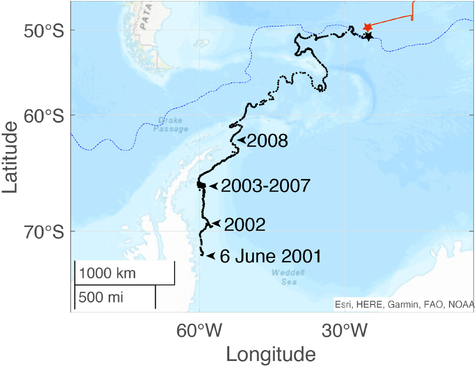
Figure 2. Track of iceberg A43f (black line) determined by satellite scatterometer, from 6 June 2001 to 21 January 2009 (data source: Budge and Long Reference Budge and Long(2018), and https://www.scp.byu.edu/data/iceberg/). The black star indicates the last recorded position for A43f on 21 January 2009. The red line shows the track of Polarstern until station 102 on 18 January 2009 (indicated by the red star). The dashed blue line marks the (climatological) position of the APF (Orsi and others, Reference Orsi, Whitworth and Nowlin1995). Black arrows show relevant positions and periods of A43f drift trajectory.
The position of the first Polarstern station in the area with broken-off glacial ice (Station 102 at 49.55∘S, 25.28∘W, 18 January 2009, 20h08) was roughly 1∘ north of the main A43f track. A43f is the only larger iceberg recorded at this time that was close to Station 102. We speculate that the broken ice field encountered by Polarstern stem from A43f, broken off probably as A43f reached its northernmost position in the Polar Front region around 5 December 2008, and, while drifting eastward toward our study area, further disintegrated into smaller pieces. According to Orsi and others Reference Orsi, Whitworth and Nowlin(1995) the APF marks the northernmost extent of the Winter Water with a temperature minimum of less than 2∘C in the upper 200 m. Our hydrographic measurements (CTD profiles down to 500 m, Fig. S1) show that our study area was located close to the APF. Stations 109 ( $\theta_{\rm min} = 1.67$∘C at p = 190 dbar) and 110 ( $\theta_{\rm min} = 1.88$∘C at p = 152 dbar) were south of the APF whereas all other stations (102-108 and 111, temperature minima above 2∘C) were in the Polar Front region.
3.2. Cooling, freshening and CO2
The broken-off glacial ice was melting fast in surface waters at (initially) about 7∘C thereby cooling the surface down to slightly below 0∘C (minimum -0.67∘C; Fig. 3b). Correspondingly, significant surface water freshening was also observed along the cruise track from the early morning of 18 January 2009 reaching a maximum of more than 2 psu at night from 18 to 19 January 2009. Salinity increased to initial values in the afternoon/evening of 19 January 2009 (Fig. 3b). The underway surface salinity measurements (Fig. 3b) can be used to define domains differing in the intensity of the perturbation:
(1) an inner core from 18 January 2009 16h to 19 January 2009 12h, in the northeastern quadrant of our study area (Fig. 3a),
(2) two narrow transitional domains sampled from 18 January 2009 3h to 18 January 2009 16h (first outer core) and from 19 January 2009 12h to 19 January 22h30 (second outer core), respectively,
(3) two unperturbed areas, south and west of our survey (17 January 2009 12h to 18 January 3h, and 19 January 22h30 to 20 January 2h, respectively).

Figure 3. a, Location of CTD stations (102–111) between 18 and 19 January 2009 (black circles) and underway salinity (colored dots) from the bow thermosalinograph of Polarstern. b, Time series (blue lines) of salinity S (upper panel), temperature T (middle panel) and surface ocean fCO2 (lower panel) from the ship’s intake at ∼11 m depth. The atmospheric fCO2 is also indicated by the red dotted line in the lower panel. The position of CTD-rosette deployments (stations) is indicated by the black arrows in the upper panel (from left to right stations 102–111). Boundaries of the domains (see text for further details) are indicated by black vertical dotted lines.
Before the freshening event, the surface water (based on observations in the unperturbed areas) was already undersaturated in CO2 (surface ocean fugacity, fCO2, around 350 µatm was smaller than the atmospheric values fCO $_2^{\rm atm}$ = 383 µatm) most probably due to the seasonal dynamics of biological production, which peaked in mid-November to mid-December, as indicated by the chlorophyll a concentrations estimated from satellite imagery (Fig. S2). Satellite imagery, however, does not indicate substantial differences in chlorophyll a values and its seasonality within the study region, as also indicated by the on-site measurements of chlorophyll a and nutrient concentrations (Fig. S3) in the perturbed (station 102) and unperturbed areas (station 111). A fertilization effect from trace metals and macronutrient input from the icebergs on surface water fCO2 can, therefore, be rejected based on the abovementioned similarities in satellite-derived chlorophyll a temporal evolution as well as in-situ chlorophyll a and nutrient measurements. In contrast, much lower underway surface fCO2 values (down to 269 µatm) were observed in areas with the strongest salinity and temperature perturbations (Fig. 3b). The surface (∼11 m depth) underway salinity measurements showed the strongest freshening in the northeast quadrant of the circular cruise track (Fig. 3a). The temperature and salinity profiles of station 105 (Fig. S4) in the inner core have been clearly affected by icebergs and the melting of glacial ice.
The disintegration of icebergs followed by fast melting of broken-off small (less than a few meters across) pieces of ice could explain the freshening and cooling of surface waters. The cooling of air above the ocean surface led to an increase in relative humidity (Fig. S5) resulting in a thick fog which made the spatial extent of the ice pieces and icebergs largely invisible. The glacial ice broken off from icebergs covered a wide size spectrum with larger pieces of typically a few meters in size (based on visual observation; Fig. 1) and thus melted much faster than the icebergs themselves, thereby cooling and freshening the surface ocean, with temperatures reaching below 0∘C. Because the temperature, T, is, to first order, linearly related to heat content (over the relevant S and T ranges, the heat capacity of seawater, cp, varies by less than 1%), S and T should be linearly related to each other, i.e.
 \begin{equation}
T(S) = \beta\, S + \beta_0 .
\end{equation}
\begin{equation}
T(S) = \beta\, S + \beta_0 .
\end{equation} The intercept, β 0, and slope, β, have been estimated from our underway data through regression of T on S and by regression of S on T (Fig. 4: red dashed lines). The regressions yield:  $\beta_{0, T\, {\rm on}\, S} = -77.1 \pm 1.3$∘C, $\beta_{T \, {\rm on}\, S} = 2.46 \pm 0.04$∘C psu−1, and $\beta_{0, S \, {\rm on}\, T} = -100.7 \pm 1.5$∘C, $\beta_{S \, {\rm on}\, T} = 3.18 \pm 0.04$∘C psu−1. The slope of the ‘geometric line’ (Draper and Smith, Reference Draper and Smith1998) crossing the centroid of the data is calculated as the geometric mean of the two regression lines, yielding $\beta_{0, {\rm geom.}} = -88.2 \pm 1.4$∘C; $\beta_{\rm geom.} = 2.80\, \pm\, 0.04$∘C psu−1, (Fig. 4, red solid line; the uncertainty of the geometric slope was estimated according to expressions given by Isobe and others Reference Isobe, Feigelson, Akritas and Babu(1990) and Babu and Feigelson Reference Babu and Feigelson(1992)).

Figure 4. Underway surface ocean salinity versus temperature. Values for the inner core correspond to the red circles. The regression (based only on inner core data) of T on S and S on T are indicated by the dashed red lines. The geometric mean of these two regressions is shown by the red solid line. Values from the transitional domain are indicated by the grey symbols (asterisks:18 January 3h00 to 16h00; crosses 19 January 12h00 to 22h30). Values for unperturbed water masses are shown by the black symbols (asterisks:17 January 12h00 to 18 January 3h00; crosses: 19 January 22h30 to 20 January 12h00).
3.3. A model for the relationship between T and S
The slope, β, and intercept, β 0 can also be estimated based on the mass, salt and energy balances yielding values that vary slightly depending on the assumption made about the iceberg core temperature (-20∘C or 0∘C). Observations of iceberg core temperatures in the North Atlantic range between -20∘C and -15∘C (Diemand, Reference Diemand1984) with the outer few meters of icebergs affected by heat exchange with the surroundings (Løset, Reference Løset1993). To the best of our knowledge, no measurements of core temperatures of icebergs in the Southern Ocean have been carried out so far; however, temperatures are expected to be close to values before calving (around -20∘C, Hartmut Hellmer, personal communication, 2011). Low (< 0∘C) ice temperatures are supported by the low water (< 0∘C) temperatures found during our study (Fig. 4). In our theoretical considerations below we therefore assume two different iceberg core temperatures representing the likely lower and upper temperature boundaries for the icebergs found in our study area, namely -20∘C for no warming during its long journey from calving to disintegration and 0∘C for warming already to the melting point. Heating pure ice from -20∘C to the melting temperature at 0∘C requires 42.2 kJ kg−1 ( $\Delta T = 20$∘C times the heat capacity of pure ice, $c_{\rm p,ice}$ ( $c_{\rm p,ice} = 2.11$ kJ kg−1∘C−1, Petrich and Eicken Reference Petrich, Eicken, Thomas and Dieckmann2010)), corresponding to 13% of the latent heat of fusion, Lm, required for the melting of ice ( $L_m = 333.4$ kJ kg−1, Petrich and Eicken Reference Petrich, Eicken, Thomas and Dieckmann2010).
The impact of ice melting on surrounding water temperature and salinity can be estimated as follows. The internal energy of seawater, E (J kg−1) is given by
 \begin{equation} E = c_{\rm p,sw} T_{\rm sw} + E_0 \end{equation}
 where T sw (∘C) is the temperature of seawater,  $c_{\rm p,sw}$ (J kg−1∘C−1) is the specific heat (or heat capacity) of seawater at constant pressure (3.985 kJ kg−1∘C−1 at S = 35, T = 7∘C, surface pressure), and E 0 is a constant that will drop out in the energy balance below (Eq. 5) The heat capacity of water, c p, varies slightly with temperature, salinity and pressure (Gill, Reference Gill1982). These small variations will be neglected here. When x kg of ice melt in y kg of seawater, mass, salt and energy balances read:
 \begin{align}
x + y = z
\end{align}
\begin{align}
x + y = z
\end{align} \begin{align}
y\, S_{\rm i} & = z\, S_{\rm f}
\end{align}
\begin{align}
y\, S_{\rm i} & = z\, S_{\rm f}
\end{align}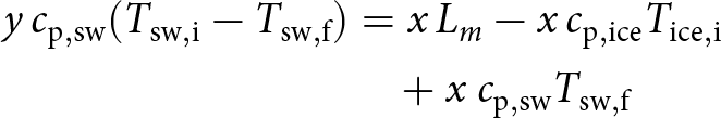 \begin{align}
y\, c_{\rm p,sw} (T_{\rm sw,i} - T_{\rm sw,f})
& = x\, L_m - x\, c_{\rm p,ice} T_{\rm ice,i} \nonumber \\ & \quad
+ x\ c_{\rm p,sw} T_{\rm sw,f}
\end{align}
\begin{align}
y\, c_{\rm p,sw} (T_{\rm sw,i} - T_{\rm sw,f})
& = x\, L_m - x\, c_{\rm p,ice} T_{\rm ice,i} \nonumber \\ & \quad
+ x\ c_{\rm p,sw} T_{\rm sw,f}
\end{align} where S i is the initial water salinity, S f is the final (after dilution) salinity,  $T_{\rm sw,i}$ (∘C) is the initial water temperature, $T_{\rm ice,i}$ (∘C) is the internal ice core temperature, and $T_{\rm sw,f}$ (∘C) is the final (after cooling) water temperature. In the balances (Eqs. 3-5) we neglect the exchange of water (evaporation, precipitation) or heat with the atmosphere. This should be a valid assumption on short time scales, despite the fact that some heat exchange with the atmosphere took place indicated by the cooling of the atmosphere leading to the formation of thick fog. For known initial salinity, S i, and observed final salinity, S f, one can calculate the glacial freshwater input:
 \begin{equation}
x = z -y = z - z \frac{S_{\rm f}}{S_{\rm i}} = z \left(1 - \frac{S_{\rm f}}{S_{\rm i}}\right)
\end{equation}
\begin{equation}
x = z -y = z - z \frac{S_{\rm f}}{S_{\rm i}} = z \left(1 - \frac{S_{\rm f}}{S_{\rm i}}\right)
\end{equation}Inserting this relationship into the energy balance (Eq. 5) leads to
 \begin{align}
z \frac{S_{\rm f}}{S_{\rm i}}\, c_{\rm p,sw} \left(T_{\rm sw,i} - T_{\rm sw,f}\right)
& = z \left(1 - \frac{S_{\rm f}}{S_{\rm i}}\right)\, \left(L_m \right. \nonumber \\ &
\left. - c_{\rm p,ice} T_{\rm ice,i} + c_{\rm p,sw} T_{\rm sw,f}\right)
\end{align}
\begin{align}
z \frac{S_{\rm f}}{S_{\rm i}}\, c_{\rm p,sw} \left(T_{\rm sw,i} - T_{\rm sw,f}\right)
& = z \left(1 - \frac{S_{\rm f}}{S_{\rm i}}\right)\, \left(L_m \right. \nonumber \\ &
\left. - c_{\rm p,ice} T_{\rm ice,i} + c_{\rm p,sw} T_{\rm sw,f}\right)
\end{align}or (z drops out and multiplication by Si)
 \begin{align}
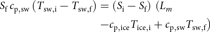
S_{\rm f} \, c_{\rm p,sw} \left(T_{\rm sw,i} - T_{\rm sw,f}\right)
& = \left(S_{\rm i} - S_{\rm f} \right)\, \left(L_m \right. \nonumber \\ &
\left. - c_{\rm p,ice} T_{\rm ice,i} + c_{\rm p,sw} T_{\rm sw,f}\right)
\end{align}
\begin{align}
S_{\rm f} \, c_{\rm p,sw} \left(T_{\rm sw,i} - T_{\rm sw,f}\right)
& = \left(S_{\rm i} - S_{\rm f} \right)\, \left(L_m \right. \nonumber \\ &
\left. - c_{\rm p,ice} T_{\rm ice,i} + c_{\rm p,sw} T_{\rm sw,f}\right)
\end{align} which is readily solved for  $T_{\rm sw,f}$
 \begin{equation}
T_{\rm sw,f} = \beta S_{\rm f} + \beta_0
\end{equation}
\begin{equation}
T_{\rm sw,f} = \beta S_{\rm f} + \beta_0
\end{equation}with
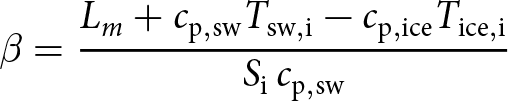 \begin{equation}
\beta = \frac{L_m + c_{\rm p,sw} T_{\rm sw,i} - c_{\rm p,ice} T_{\rm ice,i} }{S_{\rm i}\, c_{\rm p,sw}}
\end{equation}
\begin{equation}
\beta = \frac{L_m + c_{\rm p,sw} T_{\rm sw,i} - c_{\rm p,ice} T_{\rm ice,i} }{S_{\rm i}\, c_{\rm p,sw}}
\end{equation}and
 \begin{equation}
\beta_0 = - \frac{L_m - c_{\rm p,ice} T_{\rm ice,i}}{c_{\rm p,sw}}
\end{equation}
\begin{equation}
\beta_0 = - \frac{L_m - c_{\rm p,ice} T_{\rm ice,i}}{c_{\rm p,sw}}
\end{equation} The slope β (Eq. 10) has been derived as an approximation by Gade Reference Gade(1979) and is usually called the ‘Gade slope’ (e.g. Straneo and Cenedese, Reference Straneo and Cenedese2015). For  $S_{\rm i} = 33.88$, $T_{\rm sw,i} = 7.10$∘C one obtains $\beta_{\rm 0^o C} = 2.68$∘C psu−1 and $\beta_{0,{\rm 0^o C}} = -83.7$∘C assuming $T_{\rm ice,i} = 0$∘C (ice close at the melting point, from the outer layers of the iceberg) or $\beta_{\rm -20\, ^\circ C} = 2.99$∘C psu−1 and $\beta_{0,{\rm -20^o C}} = -94.3$∘C assuming $T_{\rm ice,i} = -20$∘C. Our geometric regression parameters are within the range of model-based estimates for of β and β 0 for initial ice temperatures of -20∘C and 0∘C:
 \begin{eqnarray*}
\begin{array}{ccccc}
\beta_{\rm 0\, ^\circ C} = 2.68^\circ\mathrm{C\,psu}^{-1}
& \lt & \beta_{\rm geom.} = 2.80^\circ\mathrm{C\,psu}^{-1} \\ \lt \beta_{\rm -20\, ^\circ C} = 2.99^\circ\mathrm{C\,psu}^{-1} & & \\
\beta_{0,{\rm -20\, ^\circ C}} = -94.3\, ^\circ\mbox{C}
& \lt & \beta_{0, {\rm geom.}} = -88.2\, ^\circ\mbox{C} \\ \lt \beta_{0,{\rm 0\, ^\circ C}} = -83.7\, ^\circ\mbox{C} . &&
\end{array}
\end{eqnarray*}
\begin{eqnarray*}
\begin{array}{ccccc}
\beta_{\rm 0\, ^\circ C} = 2.68^\circ\mathrm{C\,psu}^{-1}
& \lt & \beta_{\rm geom.} = 2.80^\circ\mathrm{C\,psu}^{-1} \\ \lt \beta_{\rm -20\, ^\circ C} = 2.99^\circ\mathrm{C\,psu}^{-1} & & \\
\beta_{0,{\rm -20\, ^\circ C}} = -94.3\, ^\circ\mbox{C}
& \lt & \beta_{0, {\rm geom.}} = -88.2\, ^\circ\mbox{C} \\ \lt \beta_{0,{\rm 0\, ^\circ C}} = -83.7\, ^\circ\mbox{C} . &&
\end{array}
\end{eqnarray*}3.4. Impact of dilution and cooling on fCO2
In the southern hemisphere, fCO $_2^{\rm atm}$ does not vary much on sub-seasonal times scales (and is primarily influenced by air pressure variations). The solubility of CO2 in seawater is primarily a function of water temperature, with cooling leading to large decreases of equilibrium fugacity of CO2 in seawater. In equilibrium, the fugacity of CO2 is related to the concentration of CO2 in seawater, [CO2], by Henry’s law (e.g. Zeebe and Wolf-Gladrow Reference Zeebe and Wolf-Gladrow2001)
 \begin{equation} {\rm [CO_2]} = K_0 (T,S) \cdot {\rm f_{CO_2}} \end{equation}
 where  $K_0(T,S)$ is Henry’s constant for CO2. Cooling leads to large decrease of ${\rm f_{CO_2}}$ because $K_0(T,S)$ shows strong variation with temperature (Weiss, Reference Weiss1974). In order to calculate the variations of ${\rm f_{CO_2}}$ we first estimate ${\rm [CO_2]}$ from the following initial conditions: $S_i = 33.88$ psu, $T_{\rm sw,i} = 7.10$∘C, ${\rm f_{CO_2,i}} = 351$ µatm, ${\rm TA_i}$ = 2272 µmol kg−1 (TA = total alkalinity; GLODAPv2, surface value at 49.5∘S, 24.5∘W) yielding ${\rm [CO_2]}$ = 17.1 µmol kg−1 and DIC = 2094 µmol kg−1 (DIC = dissolved inorganic carbon). Before estimating the change in fCO2 by the combined effect of cooling and dilution, we calculate the fugacity changes (sensitivities) for cooling and dilution separately:
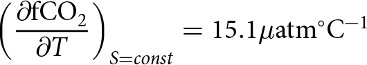 \begin{equation} \left(\frac{\partial \rm{fCO}_2}{\partial T}\right)_{S = const}
= 15.1 \mu\mathrm{atm}^\circ\mathrm{C}^{-1} \end{equation}
\begin{equation} \left(\frac{\partial \rm{fCO}_2}{\partial T}\right)_{S = const}
= 15.1 \mu\mathrm{atm}^\circ\mathrm{C}^{-1} \end{equation}and
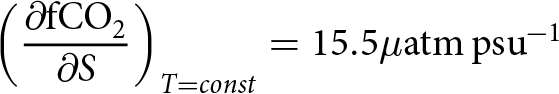 \begin{equation} \left(\frac{\partial\rm{ fCO}_2}{\partial S}\right)_{T = const} = 15.5 \mu\mathrm{atm\,psu}^{-1}\end{equation}
For the combined effect of cooling and dilution one obtains
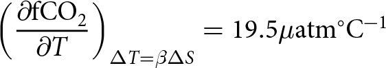 \begin{equation} \left(\frac{\partial \rm{fCO}_2}{\partial T}\right)_{\Delta T = \beta \Delta S}
= 19.5 \mu\mathrm{atm}^\circ\mathrm{C}^{-1} \end{equation}
\begin{equation} \left(\frac{\partial \rm{fCO}_2}{\partial T}\right)_{\Delta T = \beta \Delta S}
= 19.5 \mu\mathrm{atm}^\circ\mathrm{C}^{-1} \end{equation} This sensitivity ( $19.5\mu\mathrm{atm}^\circ\mathrm{C}^{-1}$) is large enough to explain the large observed perturbations in fCO2 (Fig. 3b, bottom panel) in combination with observed perturbation of T and S. All calculations were done using the CO2sys.m Version v3.1.1, 2021, https://github.com/jonathansharp/CO2-System-Extd).
3.5. Impact of disintegrating icebergs during Heinrich events
The only documented ice-sheet collapse in the Earth’s history is the release of a large armada of icebergs from the Laurentide ice sheet at the Hudson Bay, identified as the cause of the Heinrich events (Heinrich, Reference Heinrich1988) H1, H2, H4, H5 (Hemming, Reference Hemming2004). The amount of freshwater input from icebergs has been estimated to be  $0.29 \pm 0.05$ Sverdrup (1 Sverdrup = 106 m3 s−1) lasting for $250 \pm 150$ yr (Roche and others, Reference Roche, Paillard and Cortijo2004) or about $2.3 \cdot 10^{18}$ kg in total. Based on the observations from our study, we calculate a rough estimate for the potential CO2 uptake by the cooling and dilution of seawater and the re-equilibration of ocean fCO2 with the glacial atmospheric fCO2. For the sake of simplicity, we neglect re-equilibration of temperature, the fate of CO2 taken up by the ocean surface layer and feedback as, for example, the atmospheric response to surface ocean cooling (Lee and others Reference Lee, Chiang, Matsumoto and Tokos2011 and Fig. S5).
Solving the energy balance (Supplementary Material (B)) we determine that cooling 100 kg of seawater by 1∘C requires 1 kg of ice (assuming an internal iceberg temperature of -20∘C, Diemand Reference Diemand1984). Assuming that seawater with a typical total alkalinity (TA) of 2300 µmol kg−1, T = 6∘C, S = 35, is initially in equilibrium with an atmosphere of 200 µatm CO2 fugacity requires DIC = 2021.5 µmol kg−1. A cooling by 1∘C leads to a decrease of fCO $_2^{\rm oce}$ to 191.2 µatm. In order to re-equilibrate with the atmospheric fCO2 of 200 µatm, CO2 has to be taken up from the atmosphere until DIC reaches 2030.3 µmol kg−1. For the total input of glacial ice ( $2.3 \cdot 10^{18}$ kg) and the cooling capacity of glacial ice one obtains an uptake of 24 Pg C.
The addition of freshwater from melting glacial ice leads to freshening and dilution of TA and DIC. Dilution by 1% results in S = 34.65, TA = 2277 µmol kg−1, DIC = 2001.3 µmol kg−1 and thus fCO $_2^{\rm oce}$ = 196.9 µatm. Re-equilibration with the atmospheric fCO2 of 200 µatm requires the uptake of CO2 from the atmosphere until DIC = 2004.4 µmol kg−1 is reached. For the total input of glacial ice ( $2.3 \cdot 10^{18}$ kg) one obtains an additional uptake of 8 Pg C.
An uptake of 8 Pg C (or even 32 Pg C) over a time span of 250 yr would be hardly recognizable in ice core records of atmospheric CO2. However, the impact of icebergs on the hydrography (stratification, mixing; e.g. Helly and others Reference Helly, Kaufmann, Stephenson and Vernet2011; Stephenson and others Reference Stephenson, Sprintall, Gille, Vernet, Helly and Kaufmann2011) can have a significant effect on nutrient supply (via deep mixing) and primary production.
4. Discussion
The cooling and freshening of surface waters by melting of glacial ice has been extensively investigated (e.g. Helly and others (Reference Helly, Kaufmann, Stephenson and Vernet2011); Stephenson and others (Reference Stephenson, Sprintall, Gille, Vernet, Helly and Kaufmann2011) and Meire and others Reference Meire(2015), to name a few). However, our study is the first to document, by in-situ observations of hydrography and chemical parameters, impacts by fast disintegration of icebergs in the Antarctic Polar Front region. The large perturbations in temperature and salinity are due to the fact that the disintegration of icebergs took place in relatively warm waters (> 7∘C) near the Antarctic Polar Front likely leading to a very fast generation of broken-off small (< 10 m, Fig. 1) pieces of glacial ice that melt much faster than the icebergs. We not only report a unique set of temperature-salinity data but also compare the estimated covariation of salinity and temperature (T − S curve, slope β, Fig. 4, Eq. 1) with theoretical values based on the balance (conservation) of mass, salt and energy.
The investigation of melting of ice in seawater has a long history going back to experimental work by Pettersson (Reference Pettersson1878); (Reference Pettersson1900); (Reference Pettersson1904); (Reference Pettersson1907) and Nansen (Reference Nansen1906); (Reference Nansen1912). The interpretation of laboratory experiments was complicated by double-diffusion, by fast exchange of heat before the release of meltwater leading to a decrease in salinity, and by the onset of convection, depending on various experimental conditions (Gade, Reference Gade1979). The T − S slope (β) due to ice melting was calculated already by Matthews and Quinlan Reference Matthews and Quinlan(1975) who obtained a value of 2.56∘C psu−1. Their approach was criticized by Gade Reference Gade(1979) who pointed out that Matthews and Quinlan Reference Matthews and Quinlan(1975) had neglected the heat required to warm the ice to its melting temperature and the heating of the meltwater to the surrounding temperature. Based on an internal ice temperature of -10∘C and  $T_{\rm sw,i} = 3.3$∘C, $S_i = 31$ psu, Gade Reference Gade(1979) obtained a slope of 2.94∘C psu−1. These theoretical slope values depend not only on ice and water properties (Lm, $c_{\rm p,ice}$, $c_{\rm p,sw}$) but also on initial conditions ( $T_{\rm ice,i}$, $T_{\rm sw,i}$, S i; Eq. 10) and cannot be compared to each other for different initial conditions. The slope value estimated from our data, 2.80∘C psu−1, would correspond to an internal ice temperature of about -8∘C.
Freshening and cooling by glacial ice melt have opposite effects on the density of seawater. For the observed changes in T and S in our study area, the freshening effect on density is dominant. Thus, in general cooling and freshening by disintegrating icebergs at the APF reduce the density of surface waters having the potential to impact circulation and the overall CO2 sink of the Southern Ocean in the long run. This is compounded by the impact of SST on local atmospheric conditions (Fig. S5), in particular, the thick fog covering the area.
The area with reduced sea surface temperature (SST) included in our survey extended between about 25.16∘W and 25.29∘W and between 49.485∘S to 49.564∘S covering an area of about 100 km2 (Fig. S6) and is thereby larger than pixel sizes for SST determination from satellites (e.g. Merchant and others Reference Merchant2019, give 1 to 45 km2). We could, however, not see the SST signal from satellite imagery. Hence, the impact of collapsing large icebergs in the area might be overlooked when using satellite products.
Given the logistical constraints, observations on the impact of iceberg disintegration and melting are sparse. In a study of the drifting iceberg C18a in the Weddell Sea (note that C18 originated in the Ross Sea), Helly and others Reference Helly, Kaufmann, Stephenson and Vernet(2011) also recorded very low values of pCO2—down to almost 280 µatm (Fig. 2E in Helly and others Reference Helly, Kaufmann, Stephenson and Vernet2011). Helly and others Reference Helly, Kaufmann, Stephenson and Vernet(2011) and Vernet and others Reference Vernet, Sines, Chakos, Cefarelli and Ekern2011 discuss in detail the factors that could have potentially explained both the Chl a temporal dynamics and pCO2 values observed; the authors attribute the pCO2 decrease to biological production. Meire and others Reference Meire(2015), in a study of the marine carbonate system in the Godthåbsfjord and in coastal water adjacent to the Greenland Ice Sheet, also observed low pCO2 associated with glacial water input. They attributed the low pCO2 largely ( $ \gt 2/3$) to primary production and 1/3 to the input of glacial meltwater based on a laboratory end-member measurement for freshwater (FW) derived from thawing glacial ice of ( $S_{\rm FW} = 0$), DIC $_{FW}$ = $80 \pm 17$ µmol kg−1 and TA $_{FW}$ = $50 \pm 20$ µmol kg−1. The smaller TA than DIC for their FW values is not explained by the authors, suggesting that their estimates of the impact of glacial water on surface ocean pCO2 might be biased. Further, although the carbonate system was over-determined by measuring DIC, TA and pCO2 (Meire and others, Reference Meire2015), no consistency analysis is reported in the study. Henson and others Reference Henson(2023) measured DIC, TA, T and S in various Greenland fjords, but did not discuss pCO2 variations. Tarling and others Reference Tarling2024 studied the collapse of iceberg A-68A, however, they did not report any measurements of carbonate system parameters. In contrast to these previous investigations, we find that, in our study area, the impact of cooling and freshening by the melting glacial ice is large enough to explain the drop in fCO2 by up to 80 µatm (Fig. 3b). The main difference in the direct impact of glacial ice input between our and the abovementioned studies is the size of the temperature perturbation which is much larger for the rapid iceberg disintegration in the relatively warm waters at the Antarctic Polar Front. Further, the concurrence of our study with the disintegration of iceberg A43f, which was likely still ongoing, given the large amount of floating brash ice (Fig. 1), as well as the nutrient and Chl a values found on site, suggest no significant impact of changes in biological activity yet.
The combined oceanic uptake of 32 PgC during Heinrich events is possibly an overestimate as heat exchange with the atmosphere and impacts on mixed layer dynamics and circulation are not considered. Our findings show that iceberg disintegrations also affect atmospheric conditions (Fig. S5), hence, estimating the impact of Heinrich events on carbon cycling warrants further investigations using Earth System Models.
Finally, simulations of iceberg trajectories (Merino and others, Reference Merino2016; Rackow and others, Reference Rackow, Wesche, Timmermann, Hellmer, Juricke and Jung2017) included various mass loss processes (erosion by surface waves, basal melting), however, the breakup or collapse into smaller icebergs and fast-melting glacial ice with a broad range in sizes have not been taken into account. The neglect of fast disintegration processes might explain the overestimation of trajectory lengths in these simulations and has been addressed by more recent work (England and others, Reference England, Wagner and Eisenman2020). Based on our findings, the perturbation caused by disintegrating icebergs is large enough in terms of area (order of 100 km2 or more) and temperature (decrease by several degrees Celsius) to be detected by satellite and allowing to follow the evolution of the perturbed water mass. The horizontal density contrasts between the lighter (because fresher) water mass and the surrounding waters is up to 1 kg m−3 over small horizontal length scale of the order of one kilometer or less. This strong horizontal density gradient should drive a cyclonic flow around the center of the perturbed area. One could speculate that this mechanism might lead to the formation of small eddies although strong jet streams in the front region might prevent the buildup of such structures or quickly destroy them. If fast iceberg disintegrations are indeed triggered by encounters with the APF one can expect a freshwater input in the frontal zone that is larger than in adjacent waters. This freshwater input may temporally impact the dynamics and structure of the frontal region.
5. Conclusions
While steaming to the selected location for the iron fertilization experiment (LOHAFEX), we were lucky enough to encounter a field of melting glacial ice, providing us with a unique opportunity to study the ‘abnormal local conditions’ (Hardy, Reference Hardy1967) generated by the disintegration of icebergs. Our study shows that the fast disintegration of icebergs when reaching warmer conditions can lead to substantial local cooling and freshening of the ocean with considerable perturbations down to at least 75 m depth. The observed correlation between variations in temperature and salinity can be explained by a simple model based on the conservation of mass, salt and energy. As a consequence of the cooling, with additional smaller effects due to freshening, fCO2 in the study area decreased from about 350 µatm down to 269 µatm, i.e. causing a very strong undersaturation of CO2 with respect to the atmosphere. This undersaturation would lead to enhanced uptake of CO2 by the ocean. The atmospheric micro-climate generated by disintegrating icebergs might be also worth further investigation (Fig. S5). The fast disintegration of A43f was most probably triggered by temperature changes while crossing the Antarctic Polar Front (APF). If such processes are typical for icebergs in the Atlantic sector of the ACC one can expect a cumulative cooling effect and input of freshwater near oceanic fronts. The role of fronts has been only briefly mentioned in the study on iceberg evolution by Rackow and others Reference Rackow, Wesche, Timmermann, Hellmer, Juricke and Jung(2017), however, a detailed analysis is still missing. Finally, our study could shed light on the potential impacts on temperature, salinity and atmospheric CO2 by the armada of icebergs released during Heinrich events or future disintegrations of ice shelves (Hellmer and others, Reference Hellmer, Kauker, Timmermann, Determann and Rae2012).
Supplementary material
The supplementary material for this article can be found at https://doi.org/10.1017/jog.2025.10060.
Acknowledgements
Thanks to Captain of RV Polarstern Stefan Schwarze and his crew. Thanks to the chief scientists Victor Smetacek and Syed Wajih A. Naqvi, to Denis Pierrot for revising the fCO2 data. The speculation about the effect of disintegrating icebergs at glacial terminations started in a discussion with Howie Spero. Comments by two anonymous reviewers and by the editors Rachel Carr and Frank Pattyn helped us to improve the manuscript. This research was carried out under the CSIR-NIO, India supported projects NWP0014, OLP 2006, and OLP 2005. This is CSIR-NIO contribution no. 7426.
Author contributions
D.A.W.-G. wrote the first draft of the manuscript and performed most calculations, I.B. analyzed trajectories of large icebergs, G.S measured carbonate system parameters, M.G.G contributed chlorophyll data, M.V. measured hydrographic data, C.K. processed the pigment data, contributed the figures and improved the text and interpretation of the first draft. All authors discussed the results and contributed to the final version of the manuscript.
Competing interests
The authors have no competing interests.


 Open access