The integrated ice sheet response to stochastic iceberg calving

Abstract

Iceberg calving is a major source of ice loss from the Antarctic and Greenland ice sheets. However, it is still one of the most poorly understood aspects of ice sheet dynamics, in part due to its variability at a wide range of spatial and temporal scales. Despite this variability, most current large-scale ice sheet models assume that calving can be represented as a deterministic flux. In this study, we describe an approach to modeling calving as a stochastic process, using a one-dimensional depth-integrated marine-terminating glacier model as a demonstration. We show that for glaciers where calving occurs more frequently than the typical model time steps (days-months), stochastic calving schemes sampling a binomial distribution accurately simulate the probabilistic distribution of glacier state. We also find that incorporating stochastic calving into simulations of a glacier with a buttressing ice shelf changes the simulated mean glacier state, due to nonlinearities in ice shelf dynamics. Relatedly, we find that changes in calving frequency, without changes in the mean calving flux, can cause ice shelf retreat. This new stochastic approach can be implemented in large-scale ice sheet models, which should improve our capability to quantify uncertainty in predictions of future ice sheet change.

1. Introduction

Global warming is already causing sea level rise via melting of glaciers and ice sheets and ocean thermal expansion. However, future sea-level rise projections remain uncertain due to unknown future anthropogenic emissions, imperfect representation of glaciological processes in ice sheet models and internal variability that is intrinsic to the Earth system (Hu and Deser, 2013; Robel and others, 2019; IPCC, 2021). Iceberg calving is one major source of ice loss from the Greenland and Antarctic ice sheets (Rignot and Kanagaratnam, 2006; Rignot and others, 2013) and potentially the largest contributor to uncertainty in sea-level rise projections beyond 2100 (Fox-Kemper and others, 2021). Despite its importance, a comprehensive understanding of the processes responsible for calving and its accurate simulation in ice sheet models remains elusive, in part due to its variability at a wide range of spatial and temporal scales (Benn and others, 2007; 2017a; Bassis and Jacobs, 2013). Existing calving representations in ice sheet models, including simple deterministic calving laws (Benn and others, 2007), continuum damage mechanics (Duddu and others, 2013), linear elastic fracture mechanics (Yu and others, 2017) and discrete element models (Åström and others, 2013; Bassis and Jacobs, 2013), struggle to capture this variability. Calving events occur over spatial and temporal scales ranging from the multi-decadal quasi-periodic detachment of tabular icebergs hundreds of kilometers in length from floating ice shelves (Greene and others, 2022) to the detachment of icebergs meters in scales from outlet glaciers in Greenland multiple times every hour (Benn and others, 2017b; Cook and others, 2021). Such internal variability of calving over time and from glacier-to-glacier is thus challenging to reproduce in ice sheet models and is a source of unquantified ‘irreducible’ uncertainty in ice sheet projections (Bassis, 2011).

In climate and ocean models, stochastic parameterization of internal variability and unresolved processes has been used successfully to reduce systematic model errors, improve the skill of probabilistic forecasts and quantify aleatoric (i.e. due to intrinsic random variability) projection uncertainty (Porta Mana and Zanna, 2014; Berner and others, 2017; Palmer, 2019). Building a more accurate representation of calving with the inclusion of variability in ice sheet models will enable the quantification of the contribution of calving to ice sheet change and future sea level rise that can be incorporated into climate adaptation planning.

We build on the earlier work of Bassis (2011), who argued that iceberg calving can be treated as a stochastic process due to the intrinsic sensitivity of calving to unresolved micro-scale stress variations near glacier termini. In his model, the probability distribution for terminus position as a function of time is computed using simplifying assumptions, and the calving rate is calculated based on this distribution. However, Bassis (2011) only considered how the terminus position responds to such stochastic calving events, without extensively considering how the rest of the glacier integrates these stochastic calving events at the terminus, or the form of stochastic calving parameterizations. This study aims to investigate the dynamical glacier response to stochasticity in calving. Prior idealized model experiments (Robel and others, 2018; 2024; Verjans and others, 2022) tested the glacier response to treating calving flux as a Gaussian white noise process. Results from these studies show that variability in calving rates changes the glacier mean state (i.e. noise-induced drift). However, these studies did not provide a conceptual or mathematical basis for how to treat calving flux on time scales of weeks to years and did not explore the statistical dynamics of the ice flow response to this variability.

This study aims to understand multi-scale calving variability by addressing the following questions: (1) How can we accurately represent calving as a stochastic process in ice sheet models with time steps much longer than the typical duration of events? (2) How do glaciers respond to stochasticity in calving? (3) How does the stochasticity of calving affect our ability to make well-constrained predictions of future ice sheet change? In the next section, we describe the incorporation of stochastic calving into a flowline model of a marine-terminating glacier. We consider three different stochastic calving laws based on Bernoulli, binomial and Gaussian random processes. We then show that we can use a binomial random process to represent calving variability at time scales of days to years. A Gaussian random process is suitable for simulations with long time steps and high calving frequency. Both processes are equivalent to long-time-scale integrated representations of a short-time-scale threshold process (i.e. calving). In addition, we find that stochastic calving changes the mean glacier state when a buttressing ice shelf is present. We conclude by discussing how our results set the foundation for implementing stochastic calving into more complicated ice sheet models.

2. Model description

Calving is fundamentally a deterministic physical process governed by fracture mechanics which depends on small-scale stress states (Benn and others, 2007; Åström and others, 2013). As with other chaotic processes, this leads to a sensitive dependence of fracture evolution to small variation in initial conditions. Thus, in large-scale ice sheet models which do not resolve such small-scale stress states, a stochastic approach to simulating calving permits sampling of the range of possible calving event size and frequency, similar to stochastic approaches that have been used to model the range of possible states in chaotic geophysical fluid systems (Berner and others, 2017).

We start by considering a glacier that has a time-varying calving rate U_c that is typically zero but can take a non-zero value when a calving event occurs at any moment in time. We define a calving event as a period of non-zero calving rate U_c during a single model time step. This definition reflects the model’s temporal resolution and should not be conflated with instantaneous, real-world calving processes, which occur on a shorter timescale than the model resolves. The stress state and geometry of the glacier calving front produce a probability P_c for a calving event to occur at such a moment in time. A high-fidelity model of glacier fracture (e.g. Åström and others, 2013) or observations (e.g. Cook and others, 2021) may be used to quantify P_c. However, in this study, we simply assume that P_c is known a priori to investigate the consequences of such calving stochasticity on glacier evolution. In the remainder of this section, we define the mathematical model for the dynamics of this glacier and describe the specific stochastic models used to represent calving variability.

2.1. Flowline model

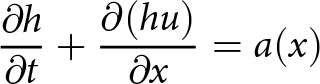
To understand the effect of stochasticity on a marine-terminating glacier in an idealized setting, we use a vertically and laterally integrated one-dimensional flowline model. Such a model is a good representation of the glacier response to stochastic calving on longer time scales and along the glacier flowline, though it does not reproduce the more complex details that may accompany realistic lateral or vertical variations in calving front geometry. As such, we restrict the scientific questions that we seek to answer to those that can be answered in such a model and leave more complex considerations for planned future work with 3D models. In this flowline model, ice thickness evolution is described by the conservation of mass

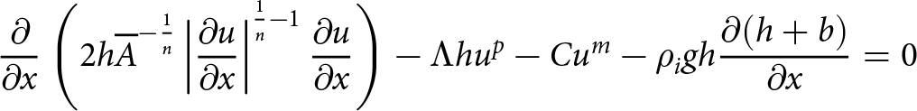
(1)\begin{align} \frac{\partial h}{\partial t}+\frac{\partial (hu)}{\partial x}=a(x) \end{align}

where h is the ice thickness, u is the ice velocity, x is the horizontal position along the direction of flow and a(x) is the surface mass balance (SMB) profile. Velocity is solved with a momentum conservation equation describing the shallow-stream/shelf approximation (SSA) with lateral shear stress included

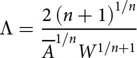
(2)\begin{align} \begin{aligned} \frac{\partial}{\partial x}\left(2h\overline{A}^{-\frac{1}{n}}\left|\frac{\partial u}{\partial x}\right|^{\frac{1}{n}-1}\frac{\partial u}{\partial x}\right)-\Lambda hu^{p}-Cu^{m}-\rho_i gh\frac{\partial (h+b)}{\partial x}=0 \end{aligned} \end{align}

where $\overline{A}$ is the vertically integrated Nye–Glen law coefficient, n is the Nye–Glen law exponent, Λ and p are lateral drag parameters, C and m are basal drag parameters, ρ_i is the ice density, g is the gravitational acceleration and b is the elevation of the bedrock above mean sea level. Following Hindmarsh (2012), Λ is calculated using

(3)\begin{align} \Lambda=\frac{2\left(n+1\right)^{1/n}}{\overline{A}^{1/n}W^{1/n+1}} \end{align}

where W is the glacier width.

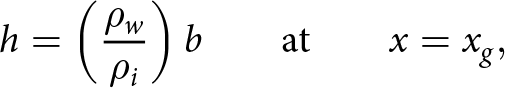
In simulated glacier states with floating ice, the grounding line position, x_g, is the location where ice begins to float, such that

(4)\begin{align} h=\left(\frac{\rho_w}{\rho_i}\right)b \quad \quad \text{at} \quad \quad x=x_g , \end{align}

where ρ_w is the density of water. We assume continuity of ice thickness, ice velocity and longitudinal stress across the grounding line. The floating ice shelf extends to the calving front $x=x_c$. The stress boundary condition at the calving front is

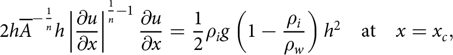(5)\begin{align} 2h\overline{A}^{-\frac{1}{n}}h\left|\frac{\partial u}{\partial x}\right|^{\frac{1}{n}-1}\frac{\partial u}{\partial x}=\frac{1}{2}\rho_i g\left(1-\frac{\rho_i}{\rho_w}\right)h^2 \quad \text{at} \quad x=x_c , \end{align}

which describes the balance of longitudinal stress with the hydrostatic and glaciostatic pressures.

The glacier may also be in a state where the calving front is grounded (i.e. no floating ice), where

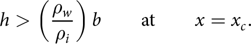(6)\begin{align} h \gt \left(\frac{\rho_w}{\rho_i}\right)b \quad \quad \text{at} \quad \quad x=x_c. \end{align}

In such cases, the stress boundary condition at the calving front is

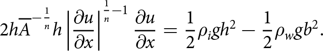(7)\begin{align} 2h\overline{A}^{-\frac{1}{n}}h\left|\frac{\partial u}{\partial x}\right|^{\frac{1}{n}-1}\frac{\partial u}{\partial x}=\frac{1}{2}\rho_i gh^2-\frac{1}{2}\rho_w gb^2 . \end{align}

In this model, the position of the calving front is defined by the balance between ice flow bringing ice mass to the front and calving removing ice mass from the front. Changes in ice flow and calving thus control the calving front position through an explicit prognostic equation for migration of the calving front:

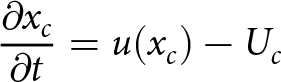(8)\begin{align} \frac{\partial x_c}{\partial t}=u(x_c) - U_c \end{align}

where $u(x_c)$ is the ice flow velocity at the calving front, and U_c is the calving rate, which is either prescribed as a constant (in deterministic simulations) or a random variable sampled from a prescribed probability distribution.

We took a similar numerical approach as Schoof 2007 in discretizing the thickness and velocity evolution equations using finite differences with a staggered grid. In order to track the calving front position, we used the stretched coordinate system (i.e. there is always a grid point at the calving front), and so

(9)\begin{align} \sigma=\frac{x}{x_c}. \end{align}

This maps the interval $0 \lt x \lt x_c(t)$ to $0 \lt \sigma \lt 1$. In cases where there is no floating ice, we used a coarse grid resolution of ∼2 km in the glacier interior and a finer resolution (∼100 m) close to the calving front to improve accuracy. In cases with floating ice, a uniform grid resolution of ∼500 m was used throughout the domain. The grounding line position can be diagnosed from the model output by finding the location where the ice thickness reaches flotation. However, the grounding line can be located between grid points. At the grid resolutions used in this study, the resulting errors in grounding line flux are less than 5% when compared to the analytical approximation of Schoof 2007. The time derivative is discretized using an implicit time step. The resulting discretized set of nonlinear equations is solved simultaneously using the Newton-Raphson method using a built-in optimization scheme in MATLAB. This computes the Jacobian numerically and solves for the unknowns at each grid point for every time step. This numerical approach ensures robust numerical stability even under stochastic calving (described in the next section), though accuracy may be influenced by the lack of higher-order differentiability in the simulated stochastic terminus position.

2.2. Stochastic calving models

We first define how the probability of calving, P_c, is modeled in our study. In the continuous framework, the evolution of probability for a calving event to occur is governed by

(10)\begin{align} \frac{dP_c}{dt} = \lambda, \end{align}

where λ is a transition rate (Bassis, 2011) which represents the probability per unit time that a calving event occurs. We obtain the probability of calving during a finite time interval ${\Delta t}$ by discretizing this continuous equation such that $P_c = {\lambda}{\Delta t}$. We investigate the use of three different types of random processes to represent stochastic calving in our model. A Bernoulli process is often used to describe an event that has a discrete number of possible outcomes, mostly commonly two: success or failure. Such a binary outcome is a good way to simulate processes undergoing changes at a threshold, such as calving events, where at a given time ice may be lost from a glacier by an iceberg of a given size detaching, or alternately, no iceberg detachment may occur. At a given time step, t_i, this is described by

(11)\begin{align} U_c(t_i)= \begin{cases} \frac{\overline{U_c}}{P_c} & \text{if } c_i=1\\ 0 & \text{if } c_i=0 \end{cases} \end{align}

where $\overline{U_c}$ is the time-averaged calving rate, $P_c = {f_c}{\Delta t}$ represents the probability of calving, f_c is the calving frequency, which can be interpreted as the transition rate in equation (10) and c_i is a sample from a Bernoulli random process. It is important to note here that we calculate P_c in terms of the time step, $\Delta t$, as a matter of numerical expediency and to ensure that for a given choice of f_c, the long-term mean calving rate, $\overline{U_c}$, will be equal to the deterministic (constant in time) calving rate from which all stochastic simulations in this study are initialized. However, as stated above, in reality, P_c is set by the small-scale stress state at the glacier front. The central assumption of modeling calving as a stochastic process is that such a probability is known a priori from high-fidelity modeling or observations. The Bernoulli process is meant to simulate individual calving events occurring with duration (seconds to days) much shorter than the typical response time scale of a marine-terminating glacier (decades to millenia; Robel and others, 2018). Even in such a reduced model, it is computationally infeasible to simulate the full glacier response at time scales of minutes or less with our intention to simulate glacier evolution over millennia. Since we are here considering a flowline model that is vertically integrated, the only individual calving events we are able to resolve are necessarily full thickness. At even the most vigorously calving tidewater glaciers, such events are sufficiently uncommon (Fried and others, 2018), that we opt to simulate the integrated glacier response to a Bernoulli random calving process with a time step of one day. Given that one day is already far in the limit of being a very short time scale compared to glacier response time scales (years to millennia), we do not expect that adopting an even shorter time step (seconds to minutes) would yield meaningful differences in such a purely viscous, depth-integrated, marine-terminating glacier model.

Even the use of the Bernoulli random calving process with a time step of one day or less is, however, not practical in large-scale ice sheet models, with typical time steps being longer for decadal-scale simulations. Some ice sheet models may also have numerical stability issues in simulating the response to large instantaneous calving events. To investigate how to implement a realistic stochastic calving scheme in a large-scale model, we also consider a binomial random calving process. A binomial random variable is the sum of n independent samples from a Bernoulli random process. Thus, on longer time steps, we can construct a binomial random calving process which has equivalent variability to Bernoulli processes sampled on shorter time steps. However, this does not guarantee that the glacier will respond equivalently to many individual calving events on daily time scales sampled from a Bernoulli process and the sum of their mass flux over weekly to yearly time scales. Thus, we aim to investigate the conditions under which these stochastic schemes produce approximately equivalent distributions of glacier state. The binomial random calving process is specified as

(12)\begin{align} U_c(t)= \frac{r\overline{U_c}}{nP_c} \end{align}

where n is the number of trials corresponding to the number of calving events within a desired time step (greater than one day), and r is a random number generated from a binomial distribution, such that $r\sim B(n, P_c)$, representing the total number of successful calving events in a given integrated time step.

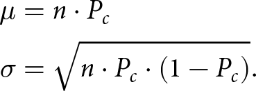
We also consider the possibility of calving as a Gaussian random process, which is commonly used in stochastic simulations (Verjans and others, 2022) and represents a limiting case of a binomial random process. This approach allows us to simulate calving as a continuous variable rather than as discrete events. The Gaussian calving rate is calculated using equation (12), where r is a random number drawn from a normal distribution with mean µ and standard deviation σ calculated as follows,

(13)\begin{align} \begin{aligned} \mu &= n \cdot P_c \\ \sigma &= \sqrt{n \cdot P_c \cdot (1-P_c)} . \end{aligned} \end{align}

In this framework, µ represents the expected number of calving events over n trials (or time steps), while σ quantifies the variability around this expected value. A key issue with using a Gaussian distribution to model calving is that it can yield negative calving velocities due to the lack of finite support. As the mean (µ) of the Gaussian distribution approaches zero, the likelihood of obtaining negative calving velocities increases (Fig. 1), which are unphysical. Even when they occur infrequently, negative velocities can lead to convergence issues in the model solver. We discuss the results from the use of a Gaussian process in Section 3.2.

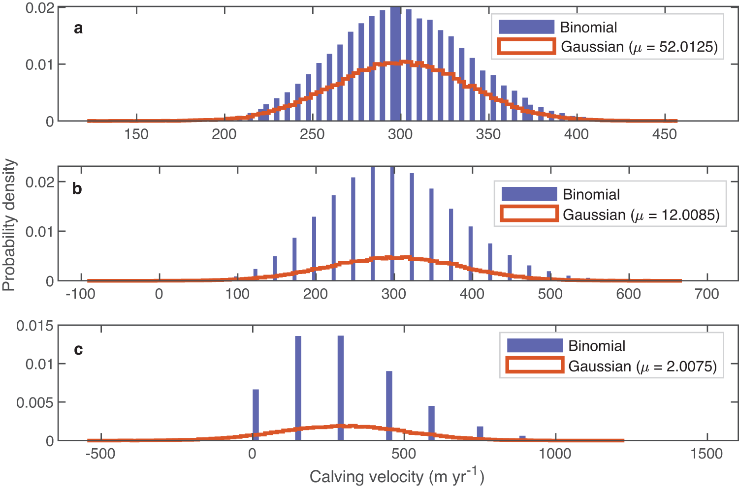
Figure 1. Comparison of binomial (blue) and Gaussian (red) stochastic calving velocity distributions over a 1 year time step for different calving frequencies: (a) 1 event per week, (b) 1 event per month and (c) 2 events per year. These frequencies result in distinct mean values µ as indicated on each plot. Histograms are across all 20 ensemble members from 4000 year tidewater glacier simulations.

2.3. Model configurations

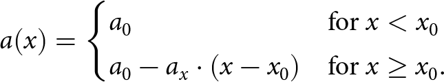
We perform two sets of idealized experiments using the model described above. The first configuration simulates a tidewater glacier with a grounded terminus, similar to outlet glaciers in Greenland. For model stability and accordance with reality, the SMB profile in this model is defined by a piecewise linear function,

(14)\begin{align} a(x) = \begin{cases} a_0 & \text{for } x \lt x_0 \\ a_0 - a_x \cdot (x - x_0) & \text{for } x \geq x_0. \end{cases} \end{align}

The SMB is 1 m yr⁻¹ through the glacier interior and decreases with position x from x ₀ (96 km) to approximately −0.7 m yr⁻¹ at the calving front. The second configuration simulates an ice shelf similar to floating ice shelves in Antarctica, where the glacier accumulates ice due to a constant SMB of 0.5 m yr⁻¹. Ice flows from the ice sheet interior towards the ocean on a prograde bed slope of $1\times 10 ^{-3}$ in both configurations. The parameter values used in both experiments are provided in Tables 1 and 2. These values are meant to be broadly representative of these kinds of glaciers but do not correspond to one specific glacier. We run the experiments to a deterministic steady state with a deterministic calving rate equal to the mean calving rate in the stochastic simulations and use the resulting steady-state conditions as initial conditions for the transient runs with stochasticity. Figure 2 shows the initial steady-state profile for the two configurations simulated by the flowline model. We run ensembles of 20 simulations for all the stochastic calving runs in this study. Each simulation within an ensemble differs only in the random realization of stochastic calving.

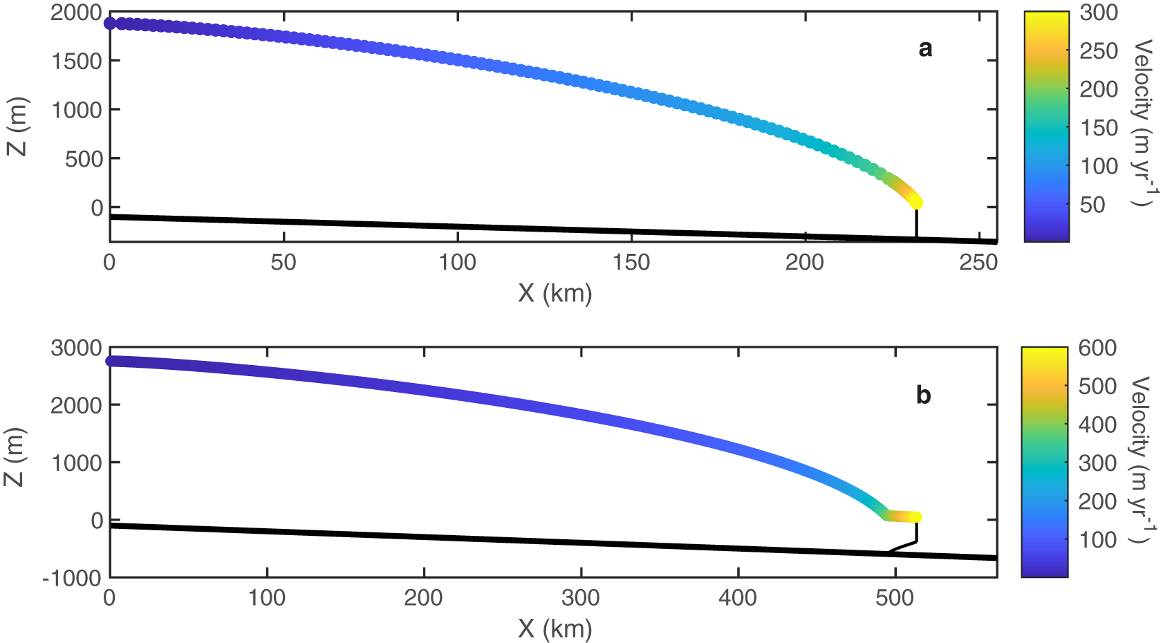
Figure 2. Initial steady-state profile for the (a) tidewater glacier and (b) ice shelf configurations simulated by the flowline model.

Table 1. List of parameters for ice shelf configuration

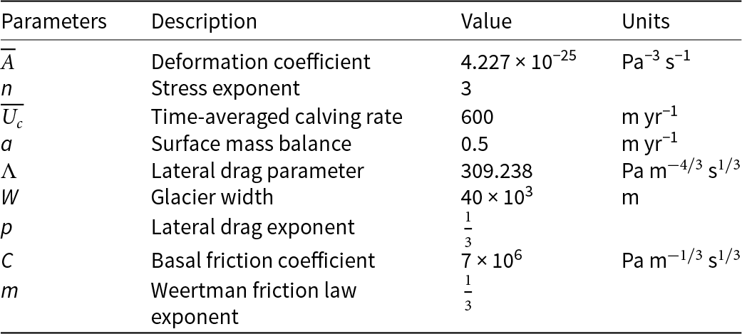
Table 2. List of parameters for tidewater glacier configuration

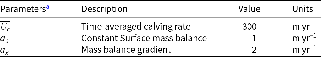
^a Parameters $\overline{A}$, n, C and m are consistent with the ice shelf configuration.

3. Results

3.1. Bernoulli and binomial stochastic calving

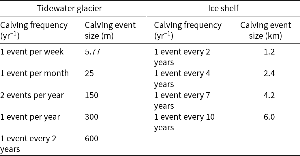
We start by comparing the distribution of glacier states produced by stochastic calving schemes based on Bernoulli and binomial random processes. Runs with the Bernoulli random calving process use a time step of one day for tidewater glacier configurations and 1 week for ice shelf configurations, both over 4000 years. We test the binomial random calving process with time steps of 1 week, 1 month and 1 year, but the average calving rate and the probability of individual calving events are the same as the Bernoulli random calving process being compared. We vary the full-thickness calving frequency, f_c, from 1 event per week to 1 event every 2 years for tidewater glacier simulations, and from 1 event every 2 years to 1 event per decade for ice shelf simulations. This variation aims to reflect the frequent calving events typical of Greenland’s outlet glaciers (Cook and others, 2021) and the infrequent calving events typical of Antarctica’s ice shelves (Greene and others, 2022). The probability of calving, P_c, is calculated by multiplying ${f_c}$ by the time step ${\Delta t}$. The calving rate at each time step is then determined using equations (11) for Bernoulli calving and (12) for binomial calving. Infrequent calving events are larger than frequent events to maintain a consistent mean calving rate, $\overline{U_c}$, between simulations. The corresponding calving event sizes for these calving frequencies, calculated by multiplying the calving rate by the time step, are listed in Table 3.

Table 3. List of parameters for tidewater glacier and ice shelf configurations

We see in Figure 3 that there are some minor quantitative differences in the distributions of glacier state for Bernoulli (blue colored bar) and binomial distributions (red, yellow and purple colored bars) in the tidewater glacier configuration. Kolmogorov–Smirnov (KS) testing indicates that such calving front distributional differences are statistically significant. However, KS testing has known issues for such large sample sizes (Sullivan and Feinn, 2012). In practice, the difference in mean calving front position is less than 200 m for the tidewater glacier configuration. Such differences are comparable to or smaller than the mesh element size of the most high-resolution simulations of marine-terminating glacier simulations. These minor differences are consistent across all calving frequencies tested. For relatively high frequencies of calving in the ice shelf configuration (Fig. S1), the binomial calving parameterization is a good approximation of the Bernoulli calving parameterization. However, this is not the case for lower calving frequencies (Figs S2 and S3). Since Bernoulli calving can be reliably simulated using normal time steps for an ice sheet model (1 week), it should be possible to reliably simulate stochastic Bernoulli calving for ice shelves in current ice sheet model configurations. Thus, we conclude that for cases where the calving is sufficiently frequent, the binomial distribution is a good approximation of Bernoulli distribution to within an error comparable to the grid resolution, and we can use an integrated binomial calving flux to accurately simulate the stochastic glacier state at various time steps. However, for infrequent calving as in ice shelf calving, Bernoulli calving is the most accurate way to stochastically simulate calving. In either case, both Bernoulli and binomial are accurate in describing the statistics of calving in time steps typical for an ice sheet model.

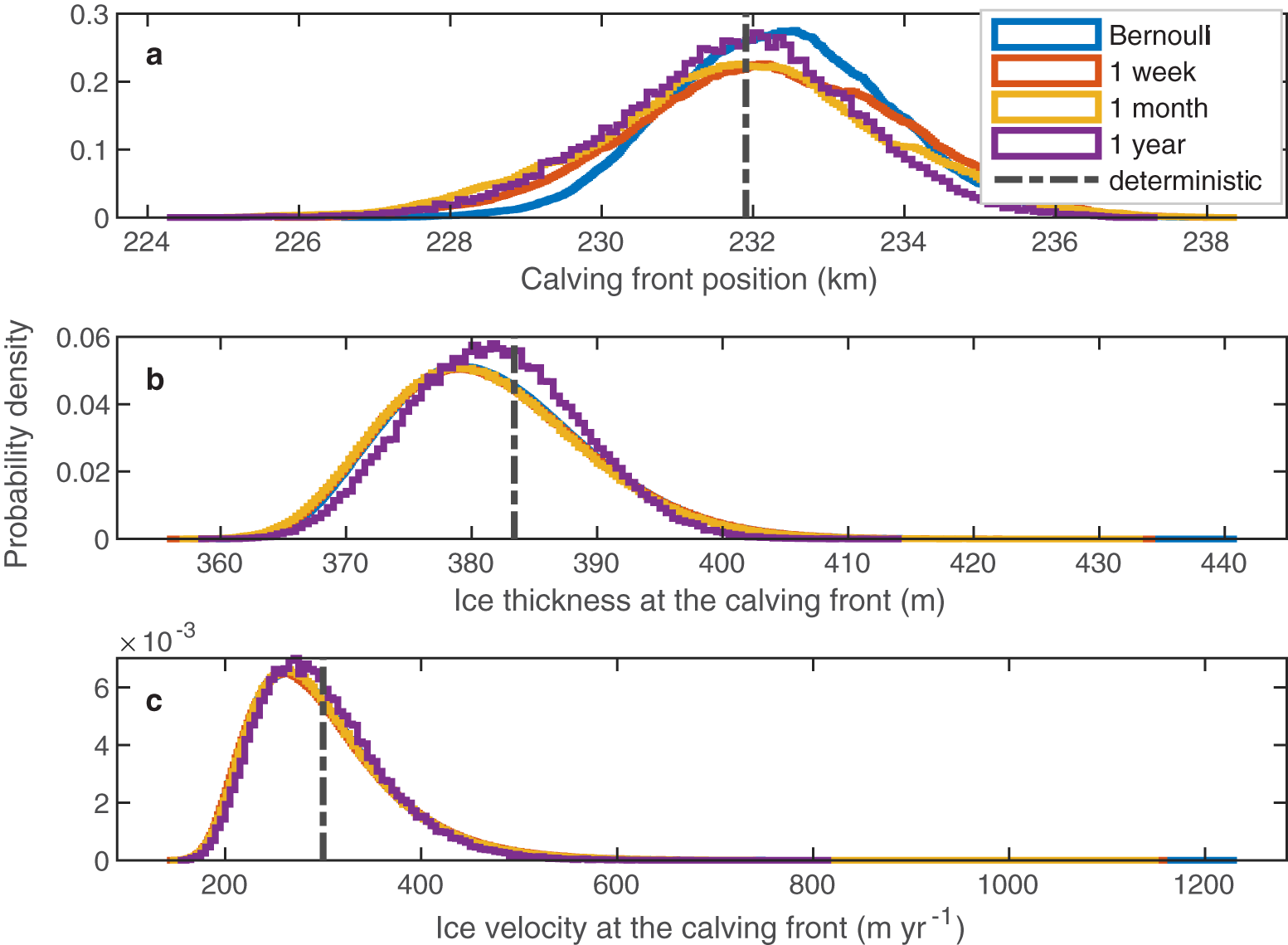
Figure 3. Distributions of (a) calving front positions, (b) ice thickness at the calving front and (c) ice velocity at the calving front from Bernoulli and binomial stochastic calving simulations for the same calving frequency (i.e. 1 event per year with a size of 300 m). Blue histogram bars are Bernoulli transient runs with a time step of one day, while red, yellow and purple histogram bars are binomial transient runs with time steps of 1 week, 1 month and 1 year, respectively. These results are from 4000 year tidewater glacier simulations across 20 ensemble members.

3.2. Gaussian calving simulations

We also run simulations of stochastic calving using a Gaussian random process, which has previously been used in stochastic ice sheet modeling (Verjans and others, 2022; Robel and others, 2024). We vary the calving frequency from 1 event per week to 1 event every 2 years for comparison with Bernoulli and binomial tidewater glacier simulations. To address the issue of negative calving velocities from Gaussian process preventing convergence of the model solver, we truncate the Gaussian by setting a zero minimum calving velocity. In Figure 4, we show the distribution of calving front position from Gaussian calving simulations alongside equivalent Bernoulli and binomial simulations for two specific calving frequencies: 1 event per week and 2 events per year. The corresponding calving velocity distributions are shown in Figure 1a for 1 event per week and Figure 1c for 2 events per year. We see that for a calving frequency of 1 event per week (Fig. 4a, the glacier states simulated by the Bernoulli (blue line), binomial (red line) and Gaussian (yellow line) calving processes are similar. However, as the frequency decreases, as seen in the case of 2 events per year (Fig. 4b), the glacier state that is simulated from the Gaussian simulation shows a significant difference from the Bernoulli and binomial glacier states. This is due to the truncation of the calving velocity distribution qualitatively changing the leading-order statistical moments of this distribution. The mean ensemble calving velocity increases to 334 m yr⁻¹, the standard deviation decreases and the skewness increases. In the ice shelf cases, where calving frequencies are relatively low, the resulting small mean (µ) values also led to frequent occurrences of negative calving velocities, preventing model convergence. We discuss the implications of these results for ice sheet modeling further in Section 4.

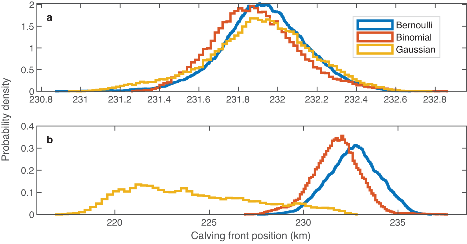
Figure 4. Distributions of calving front positions from Bernoulli (blue line), binomial (red line) and Gaussian (yellow line) stochastic calving tidewater glacier simulations over 4000 years. Bernoulli transient runs have a time step of one day, while binomial and Gaussian runs have time steps of 1 year. Shown are (a) 1 event per week with µ = 52.0125 and (b) 2 events per year with µ = 2.0075.

3.3. Distribution of calving front position

In another ensemble of simulations, we vary the calving frequency without changing the average calving flux to determine the influence of calving style on the distribution of the calving front position. We compare the stochastic tidewater glacier and ice shelf simulations with their deterministic simulations in Figure 5. The spread and skewness of the distribution of glacier state change as a function of calving frequency in both configurations. As calving events become more frequent, the spread of the distribution decreases approximately as a square root of the calving frequency (indicated by the solid line in Fig. 6). This is to be expected, as the standard deviation (σ) of the binomial/Gaussian random calving velocity as defined in equations (12) and (13) should vary like $\sigma_{U_c} \propto P_c^{-\frac{1}{2}}$. Put another way, the uncertainty in the simulated glacier state (as measured by the standard deviation) due to calving variability is set by the calving frequency. So, glaciers with less frequent (and larger) calving events are subject to more irreducible uncertainty in their simulated state.

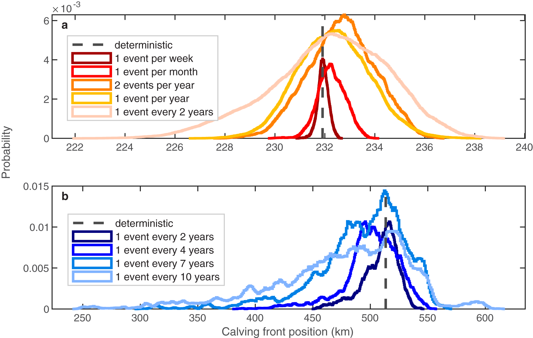
Figure 5. Distribution of calving front positions after 4000 years for different calving frequencies: (a) Bernoulli tidewater glacier runs and (b) Bernoulli ice shelf runs. The black dashed lines in both figures are deterministic steady-state initial conditions.

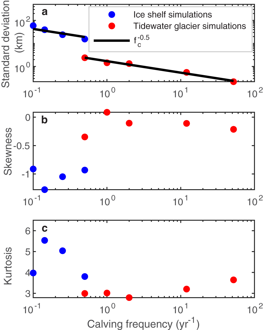
Figure 6. (a) Standard deviation, (b) skewness and (c) kurtosis of the distribution of calving front positions (from figure 5) plotted against calving frequencies. Blue points are tidewater glacier runs, and red points are ice shelf runs.

The shape of the distributions also shows increasing skew as we move to lower calving frequencies, with more pronounced skewness in the ice shelf cases (Fig. 5b) where calving frequencies are very low. These asymmetries arise because infrequent large calving events lead to significant jumps in the calving front position. With infrequent calving, the glacier has more time to advance, resulting in larger ice loss when calving does occur, which skews the distribution. In contrast, more frequent events result in smaller, more regular changes, leading to a more symmetric distribution. This is further illustrated by the plot of skewness and kurtosis shown in Figure 6b and c. Though there are also analytical predictions for the skewness and kurtosis of binomial distributions as a function of P_c, these appear to be less predictive of these moments in glacier state distribution, due to the effect of glacier dynamics. This increase in the spread and skewness of the probability distribution of the calving front positions as calving events become larger and less frequent is consistent with findings in Bassis (2011), which showed that this is unavoidable when calving event sizes are not negligible compared to the system size.

3.4. Realistic calving size distribution

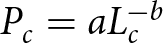
Thus far, we have explored the glacier response to idealized stochastic calving with a single event size. We now consider a more realistic size distribution for calving, in order to determine whether large and infrequent or small and frequent calving events exert a stronger control on the distribution of glacier state. Åström and others (2021) and other studies (Tournadre and others, 2016; Sulak and others, 2017; Crawford and others, 2018; Scheick and others, 2019) have found, both in theory and observations, that recently calved icebergs follow a power-law distribution. This distribution is attributed to the physical processes that cause fragmentation of brittle materials. To model such a polydisperse distribution of calving event sizes in the tidewater glacier configuration, we define the probability of calving, P_c, as a power-law function of calving events size

(15)\begin{align} P_c = a L_c^{-b} \end{align}

where a is a normalization constant that we use to ensure a constant mean calving rate, b is the power-law exponent and L_c represents the calving event size in terms of along-flow dimension of the calved iceberg, since all calving events in our depth-integrated model are full-thickness events. We vary the calving event size across discrete values: 5.77, 8.33, 12.5, 25, 50, 150, 300 and 600 m. These sizes are calculated by multiplying the calving velocities from different calving frequencies by the time step (i.e. calving size $L_c = U_c\Delta t$). At each time step, we simulate a finite number of independent Bernoulli processes, one for each calving event size. For each size, we calculate the probability P_c using equation (15) and perform a random draw from the Bernoulli process to determine whether a calving event occurs for that size. The normalization factor a is calculated once before the Bernoulli random draw. We then calculate the calving rate $U_c(t)$ at time step t as the sum of sizes of calving events that occur, divided by the time step. We test different power law exponents b (1, 1.5, 2, 2.5 and 3) over a range spanning those found in observations and theory. The resulting distributions (colored solid lines) are compared against two cases from single-event-size Bernoulli calving simulations for a tidewater glacier: the most frequent event (1 event per week, shown as red dashed lines) and the least frequent event (1 event every 2 years, shown as black dashed lines) in Figure 7. All simulations plotted in Figure 7 have the same mean calving rate. As b increases, the distribution of glacier calving front position approaches that of the single-event-size simulations with frequent calving, indicating that small and frequent calving events dominate the glacier response. In contrast, b = 1 appears furthest from the frequent small event distribution, indicating a more balanced contribution of calving event sizes to setting the glacier state. We can make sense of this by considering the expected value of calving event size

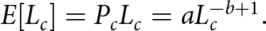(16)\begin{align} E[L_c] = P_c L_c = a L_c^{-b+1}. \end{align}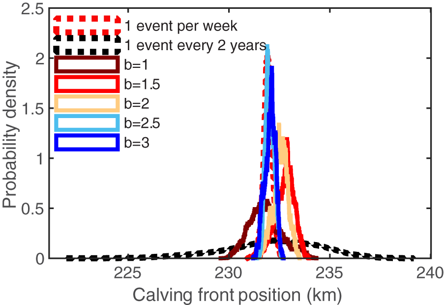

Figure 7. Comparison of calving front position distributions from tidewater glacier simulations with realistic power-law calving size distributions to two cases of single-event-size Bernoulli simulations. Red with a frequency of 1 event per week. Black dashed line is single-event-size calving simulations with a frequency of 1 event every 2 years. Colored solid lines correspond to different power law exponents, b, simulations (specified in equation (15)).

This essentially measures the average contribution from each calving event size to the overall calving rate at every point in time, taking into account the size and probability of different types of calving events. The expected value predicts that when b > 1 small events contribute more than large events to the overall calving flux, and the larger b is, the more important small events are. For b = 3, the average contribution of small calving events (i.e. $L_c = 10$ m) to the total calving flux will be 100 times greater than the contribution of large events (i.e. $L_c = 100$ m). Prior observations (Sulak and others, 2017; Crawford and others, 2018; Scheick and others, 2019; Åström and others, 2021) strongly indicate that $1\leq b \leq 3$ in reality, and thus we expect the distribution of glacier state to mainly be set by the stochastic variability of small calving events.

3.5. Noise-induced drift

To investigate the impact of variations in calving frequency on the mean glacier state, we vary the calving frequency in an ensemble simulation while maintaining a constant mean calving rate. We conduct a two-phase experiment in our model with the ice shelf configuration. We focus on the ice shelf configuration because the distributions of glacier state plotted in the long-running experiments plotted in Figure 5 indicate a shifted mean in the ice shelf configuration, but not the tidewater glacier configuration. Initially, we run ensemble simulations with a calving frequency of 1 event per month for 6000 years. Following this, we decrease the calving frequency to 1 event every 10 years (keeping mean calving rate the same) and continue the simulation for an additional 2000 years.

We plot the time series of calving front position for the ensemble mean and individual ensemble members in Figure 8, contrasting the effects of the two distinct calving frequencies. While there is an apparent change in the ensemble-average glacier calving front position (long thick blue line), it is relatively small (3 km over 6000 years). The retreat rate then accelerates when calving frequency is reduced to 1 event every 10 years (thick red line). We initialize two additional 1000 year ensemble simulations from a single ensemble member of the low-frequency (1 event every 10 years) simulation at years 6500 and 6700, increasing the calving frequency in those simulations back to 1 event per month. Following this increase, the ice shelf tends towards a longer steady-state position with a reduced retreat rate (short blue lines). We remind the reader that throughout this entire simulation, the mean calving rate remains constant at the same level as in the initial deterministic steady-state. Thus, it is solely the change in stochastic variability that drives these retreats, with higher retreat rates for lower calving frequency.

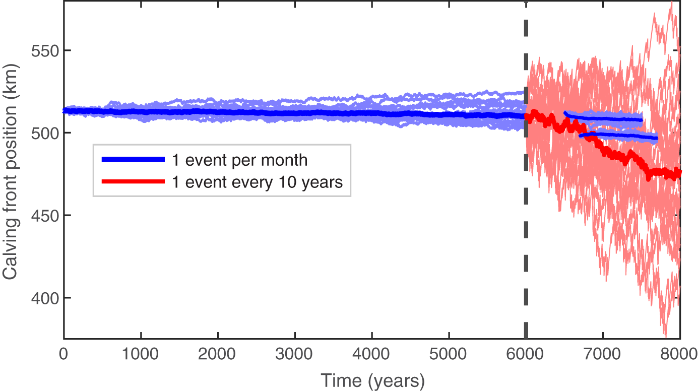
Figure 8. Calving front position change in response to variations in calving frequency, simulated using an idealized ice shelf configuration. Thick blue and red lines are ensemble means for simulations with a calving frequency of 1 event per month and 1 event every 10 years, respectively. Thin lines are 20 individual ensemble members. The black dashed line marks the transition from high to low frequency at year 6000. The two short blue lines in the rightmost part of the plot are ensembles that were initialized from a single ensemble member of the low-frequency simulation at years 6500 and 6700, with calving frequency changed back to 1 event per month.

These results are consistent with Verjans and others (2022) and Robel and others (2024), which also found that noise-induced drift can occur in 2D ice sheet models for glaciers with buttressing ice shelves, or in tidewater glacier simulations when there are identifiable reverse-sloping regions of bed topography. Robel and others (2024) also showed mathematically that we expect stochastic calving to increase the time-averaged ice flow velocity through the buttressed grounding line, leading to retreat when initialized from a deterministic steady-state or a statistical steady-state with less calving variability. In contrast, we do not find detectable drift for tidewater glacier configurations without regions of reverse-sloping bed topography, which add bifurcations to the system dynamics, as shown in Robel and others (2024).

3.6. Decadal-scale calving front migration due to natural calving variability

To further investigate the role of stochastic variability on retreat rates, we analyze the distribution of calving front position changes over different time intervals. We run ice shelf simulations for 10 000 years to achieve a statistical steady state. In the simulations with 1 calving event per month, the ice shelf comes very close to a statistical steady state. However, in simulations with less frequent calving events (1 event every 2 years and 1 event every 7 years) the calving front positions drift towards an ice-free state ( $x_c = 0$ km), rather than reaching a steady-state with some ice. This is likely a product of the assumption that the mean calving rate remains constant. We subsample each ensemble at monthly and yearly intervals to resemble observations of calving front positions. We plot histograms of ensemble trends over 5, 10 and 20 year intervals for the three calving frequencies in Figure 9 (for monthly sampling of calving front position) to examine variability in migration rates. Focusing on the 10 year trends (middle plots), we find that for the very frequent calving event (dark blue bars), where the mean is slightly offset from zero (−0.1437 m yr⁻¹), migration rates due to stochastic variability are relatively small, falling within a range of tens of meters per year. In contrast, simulations with less frequent calving (light blue and cyan bars) show a much wider range of migration rates. While there are non-zero mean migration rates in these cases of −0.2010 m yr⁻¹ for 1 event every 2 years and −0.8140 m yr⁻¹ for 1 event every 7 years, stochastic variability leads to a significant spread in migration rate around the mean, producing periods of retreat at rates of up to hundreds of meters per year that are not caused by any mean forcing. We observe similar patterns in the yearly data (Fig. S4), but with even more pronounced migration rates. In Figure 10, we compare histograms of ensemble trends over 5 year intervals for calving front positions sampled at weekly, monthly, yearly and 5 years (using only the end points) intervals from the simulations with 1 event every 7 years. Weekly sampling produces the lowest migration rates of just a few meters per year while sampling at every 5 years yields rates of up to several kilometers per year. We further discuss the implications of such results for making statistically robust statements about observed calving front retreats in the next section.

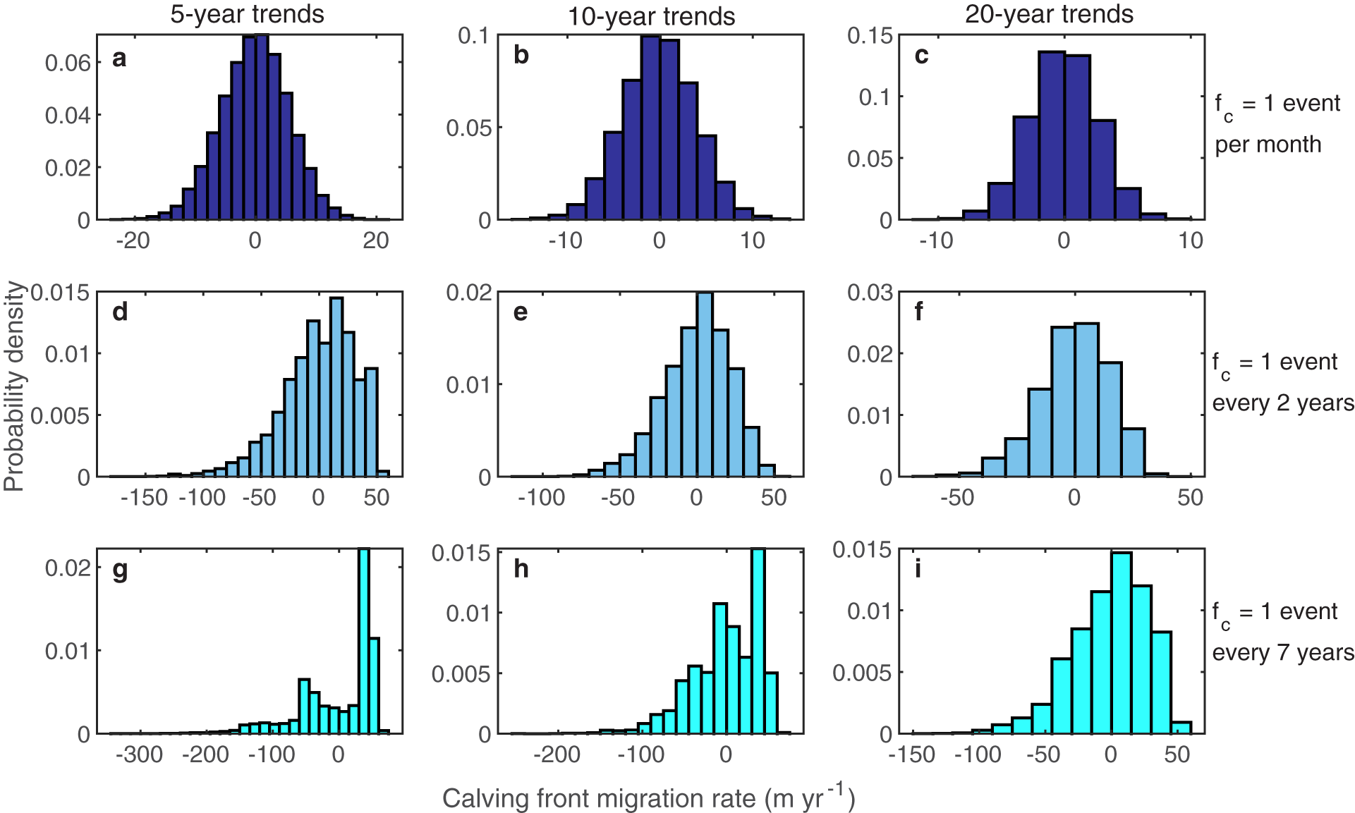
Figure 9. Histograms of ensemble trends over 5 year (left column), 10 year (middle column) and 20 year (right column) intervals for ice shelf simulations with different calving frequencies. Each row represents a different calving frequency: dark blue bars for 1 event per month (a)–(c), light blue bars for 1 event every 2 years (e)–(f) and cyan bars for 1 event every 7 years (g)–(i). Negative migration rates indicate calving front retreat, while positive migration rates indicate calving front advance. Results are from subsampling at monthly intervals.

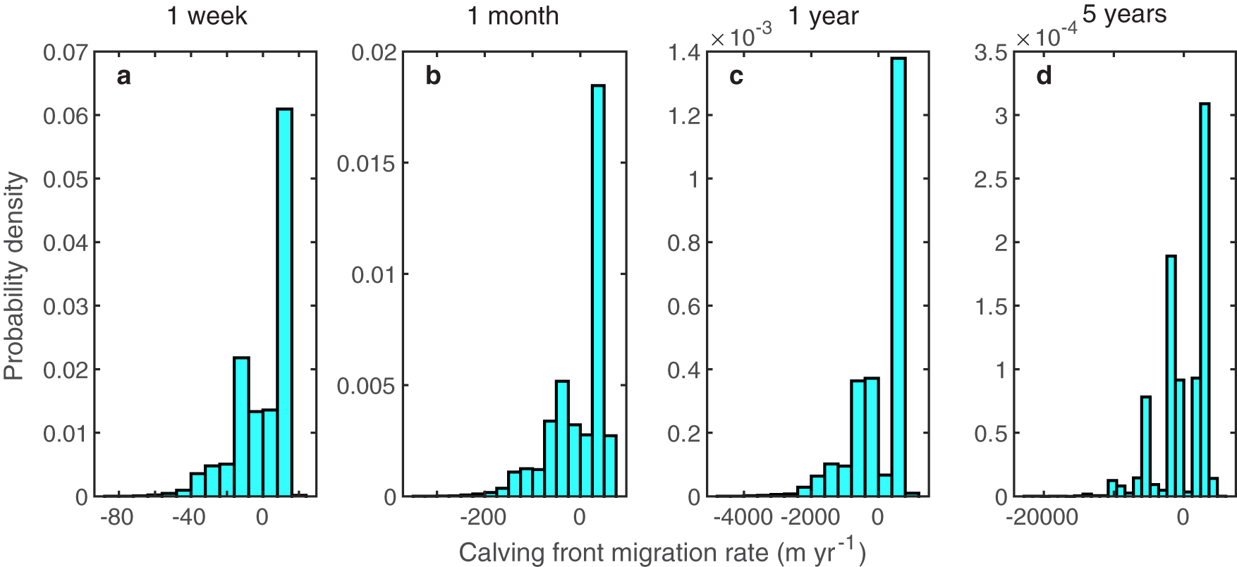
Figure 10. Histograms of ensemble trends over 5 year intervals with sampling of calving front positions at different temporal resolutions: (a) 1 week, (b) 1 month, (c) 1 year and (d) 5 years. Negative migration rates indicate calving front retreat, while positive migration rates indicate calving front advance. All histograms are from ice shelf simulations with the same calving frequency, 1 event every 7 years.

4. Discussion

In this study, we treat calving as a stochastic process in idealized simulations of marine-terminating glaciers. Our primary goal is to better represent calving variability in ice sheet models and understand the effects of calving on the natural distribution of glacier state. We find that a Bernoulli or binomial random process can be used to accurately represent the stochastic nature of sporadic calving events, while using time step lengths used in many ice sheet models, typically weeks or months. In contrast, a Gaussian random process can closely approximate the binomial process only at high calving frequencies and long time steps. A binomial distribution tends to a Gaussian distribution when the number of calving events per time step is large and the calving probability on each time step is neither close to 0 nor 1. This approximation is justified by the Central Limit Theorem, which states that the distribution of the sample mean approaches a normal distribution as the number of trials increases, provided that event probability is not very close to 0 or 1 (Blitzstein and Hwang, 2019). However, when calving probability is very low (i.e. infrequent calving) or very high, the binomial distribution becomes skewed, as shown in Figure 1c, which the Gaussian approximation fails to capture accurately. Furthermore, truncating the Gaussian distribution to exclude negative calving velocities alters its statistical properties and changes the mean calving velocity. Therefore it is crucial to consider the impact of truncation on model accuracy when using Gaussian processes. Our recommendation is thus to use a Bernoulli or binomial random process to represent calving variability in ice sheet models where feasible. We note that in reality, f_c may vary over time in response to changing glacier dynamics and climate forcing. Future work could explore how a time-varying binomial approximation compares to the Bernoulli approach.

Simulating variability in glacier state using a more realistic power-law calving size distribution, indicates that the distribution of glacier state is set by smaller events for power-law exponents greater than 1. This also demonstrates that composite stochastic calving laws with long time steps can be constructed directly from observed calving event size catalogs. For calving styles that we expect in reality, the smallest events are likely to dominate the mass flux and therefore the glacier state distribution. However, this conclusion likely does not hold for ice shelves where calving occurs mainly through very large, very infrequent events. Such cases may be better represented through single-event-size stochastic calving parameterizations.

Figure 8 shows that changes in the calving style and size distribution can modify the mean glacier state (i.e. the noise-induced drift) when a buttressing ice shelf is present. This drift tendency depends on the nature of calving, with the ice shelf tending to zero length when calving events are large and infrequent. This occurs because the calving probabilities are independent of the ice shelf size, allowing large icebergs to break off even when the shelf is short. Since velocity decreases with decreasing shelf length, infrequent but large calving events drive further retreat suggesting a potential feedback between buttressing and noise-induced drift from stochastic calving.

If an ice shelf starts to calve more frequently, an increase in the overall average calving flux will typically cause it to retreat. However, an important finding of this study is that an increased frequency of calving events can shift the system toward a longer steady-state glacier compared to less frequent calving, as shown in Figure 8. Thus, accurate representation of stochasticity is crucial to simulating both the mean state and the response of marine ice sheets to changes in calving flux and style. As argued by Robel and others (2024), models that do not include stochasticity are intrinsically biased with potential impacts on their modeled sensitivity to future climate change.

Histograms of trends in calving front position show that we should expect transient periods of calving front retreat or advance due to random chance. The probability that we observe a retreat due to random chance is higher in simulations with infrequent events. Our results also show that the frequency and size of calving events play a key role in determining how much uncertainty in our predictions can be reduced or constrained. Glaciers with large, infrequent calving events are subject to more irreducible uncertainty. Previous studies (Baumhoer and others, 2021; Greene and others, 2022; Andreasen and others, 2023) have observed km-scale calving front retreats over decadal time scales, attributing these changes to internal ice dynamics, geometry and external environmental and mechanical forcing, depending on the period and region. Our work shows that we need to account for the role that natural calving variability may play when analyzing trends in calving front retreat. Making accurate statistical inferences about the significance of these trends requires methods that can generate realistic null hypotheses, and our model and parameterization enable such analysis. We also find that infrequent observations of calving fronts are more likely to produce spurious observations of retreat, emphasizing the importance of having an observational platform that can observe calving front position data at least as frequently as monthly time scales.

Our modeling approach, while promising, has some limitations that must be considered. While the use of a one-dimensional flowline model is well-suited for capturing glacier response to calving on longer timescales along the flowline, it does not resolve the complexities introduced by lateral or vertical variations in calving front geometry. The extent to which these variations might influence our conclusions remains uncertain and requires further investigation. Adapting ideas from this study to two-dimensional ice sheet model simulations requires new considerations. Our approach is purely statistical in nature and thus does not fully capture the actual physics of fracture which tends to affect calving front geometry (Benn and others, 2007). A critical question then arises regarding whether calving events at each point within a given glacier can be treated as stochastic independent draws from a distribution, or if they are correlated. This correlation, driven by physical processes along the glacier front, influences the complex patterns observed at the calving front that cannot be fully captured by a stochastic model assuming complete independence across all points in the mesh. One possible way forward is to use spatio-temporal calving rates from observations to constrain the calving statistics in a 2D model.

We also assume a known distribution of calving variability. This assumption, while reasonable for our current understanding of calving processes, may not fully capture the uncertainties inherent in calving behavior. Addressing this limitation necessitates extensive data on calving rates to constrain our calving probability distribution, making this approach more viable and applicable to realistic simulations. An alternative would be to introduce stochasticity in parameters within existing calving parameterizations such as the Von Mises calving law, a calving law based on a threshold in local glacier stress (Morlighem and others, 2016). This approach would allow for dynamic feedback between calving rates and glacier geometry, while still capturing the inherently stochastic nature of glacier calving behavior.

5. Conclusion

Stochastic parameterizations of glaciological processes, like calving, in large-scale ice sheet models can be used to quantify the effects of internal variability in such a process on ice sheet simulations. In this study, we treat calving as a stochastic process in a marine-terminating glacier system to better understand how to implement such parameterizations in ice sheet models, and the effect of representing this internal variability on the glacier system. We demonstrate that stochastic calving can be readily incorporated into viscous ice sheet models with long time steps through the use of binomial or Gaussian random processes, without the need to resolve individual calving events. Results from this study also show that stochastic calving parameterization changes the mean glacier state in glaciers with buttressing ice shelves. This indicates that the retreat of ice shelf calving fronts is the result of both the mean size and frequency of calving events. We also find that for calving styles expected in tidewater glaciers, smaller events dominate the mass flux and strongly influence the glacier state. This new approach to modeling calving provides a framework for implementing stochastic calving capabilities in large-scale ice sheet models, which should improve our capability to make accurate predictions of future ice sheet change with quantified uncertainties.