


1. Introduction
Due to heavy irrigation and high domestic water demand in the Amu Darya basin, the Pamir mountains play a crucial role for downstream freshwater supply (Pohl and others, Reference Pohl, Gloaguen, Andermann and Knoche2017, Immerzeel and others, Reference Immerzeel2020). The Amu Darya basin contains more than  $10\,000\,\mathrm{km}^2$ of glaciers that provide around 5.5 ± 1.9 Gt of meltwater every year (Pritchard, Reference Pritchard2019, Miles and others, Reference Miles, McCarthy, Dehecq, Kneib, Fugger and Pellicciotti2021). Glaciers located on the Pamir mountains are close to (or within) the so-called ‘Karakoram anomaly’ (Hewitt, Reference Hewitt2005, Farinotti and others, Reference Farinotti, Immerzeel, de Kok, Quincey and Dehecq2020). This anomaly is originally defined by near-zero or positive glacier mass balances for the beginning of the 21st century, and its definition was extended to the previous decades (Bolch and others, Reference Bolch, Pieczonka, Mukherjee and Shea2017, Zhou and others, Reference Zhou, Li and Li2017). While it is clear that eastern Pamir glaciers have been in a balanced state at least since 1970, the mass balances of the western and central Pamir glaciers are more negative (Brun and others, Reference Brun, Berthier, Wagnon, Kääb and Treichler2017, Lin and others, Reference Lin, Li, Cuo, Hooper and Ye2017, Zhou and others, Reference Zhou, Li, Li, Zhao and Ding2019, Shean and others, Reference Shean, Bhushan, Montesano, Rounce, Arendt and Osmanoglu2020, Bhattacharya and others, Reference Bhattacharya2021, Hugonnet and others, Reference Hugonnet2021). Diverging estimates exist in the literature about recent mass balances in the western and central Pamir (Gardelle and others, Reference Gardelle, Berthier, Arnaud and Kääb2013, Kääb and others, Reference Kääb, Treichler, Nuth and Berthier2015), even though the most recent ones point toward mass losses (Hugonnet and others, Reference Hugonnet2021), which would thus exclude these regions from the anomaly.
Geodetic mass-balance estimates provide region scale estimates of glacier mass balances over multiple years and should be complemented by field studies to better understand the variability of mass balances and their link with meteorology and climate. There is a large temporal gap in ground-based glacier monitoring in Central Asia following the collapse of the Union of Soviet Socialist Republics (USSR). Most scientific activities in this region were abandoned in the 1990s, with some of them being re-established in the past years (Hoelzle and others, Reference Hoelzle2017). This gap is being partially filled in the north-western Pamir (Pamir Alay) by the re-interpretation of firn cores and profiles collected in the 1970s, combined with modeling of glacier mass balance (Barandun and others, Reference Barandun2015, Kronenberg and others, Reference Kronenberg, Machguth, Eichler, Schwikowski and Hoelzle2021, Reference Kronenberg, van Pelt, Machguth, Fiddes, Hoelzle and Pertziger2022). In the eastern Pamir, the mass balance of Muztag Ata No. 15 Glacier was reconstructed from 1980 to 2017 (Zhu and others, Reference Zhu2018). All these studies found a pattern of increasing accumulation on glaciers during the last 40–60 years together with an increased melt, that explain relatively stable mass balance in the region, at least for the higher elevations (Zhu and others, Reference Zhu2018, Kronenberg and others, Reference Kronenberg, Machguth, Eichler, Schwikowski and Hoelzle2021, Reference Kronenberg, van Pelt, Machguth, Fiddes, Hoelzle and Pertziger2022, Machguth and others, Reference Machguth2024).
Still, in the western and central Pamir, data remain scarce. Scientific activities focused on the longest mountain glacier in the region: Fedchenko Glacier (now called Vanjyakh), located in Tajikistan. The long-term mass balance of the glacier was calculated for the period 1928–2000 (Lambrecht and others, Reference Lambrecht, Mayer, Aizen, Floricioiu and Surazakov2014) and 1975–99 (Zhou and others, Reference Zhou, Li, Li, Zhao and Ding2019). However, these studies are limited by the lack of high quality topographic data in the upper part of the glacier area that are hampered by penetration issues for the X- and C-band radar data (Rignot and others, Reference Rignot, Echelmeyer and Krabill2001, Dehecq and others, Reference Dehecq, Millan, Berthier, Gourmelen, Trouvé and Vionnet2016, Lambrecht and others, Reference Lambrecht, Mayer, Wendt, Floricioiu and Völksen2018) and by saturation issues for the optical data, leading to incomplete coverage. GNSS data partially compensate these disadvantages, thanks to their high precision, but they are not acquired frequently and provide only a partial coverage, being thus difficult to compare to other data sources. We identify a need to process all the existing topographic data into a consistent framework to document decadal elevation changes.
In this study, we re-visit topographic data from 1928 and 1958 acquired by the Russian–German expedition of 1928 and by the Academy of Sciences of the Uzbek Republic expedition of 1958 (Lambrecht and others, Reference Lambrecht, Mayer, Aizen, Floricioiu and Surazakov2014, and references therein). We combine these data with a digital elevation model (DEM) derived from KH-9 imagery from August 1980, a SPOT5 DEM from November 2011, Pléiades DEMs acquired in fall 2017, summer and fall 2019 and fall 2021, ICESat data from fall 2003 and GNSS data from August 2009, 2015, 2016 and 2019. The series of glacier elevation change is then analyzed in light of temperature and precipitation changes from weather station data and reanalysis products (ERA5).
2. Study area
Fedchenko Glacier is the largest glacier in Central Asia, with an area of  $700\,\mathrm{km}^2$ (Windnagel and others, Reference Windnagel2023). It is also famous for being one of the longest glacier in Asia, with a center line longer than 75 km (RGI Consortium, 2023). Fedchenko Glacier is a winter-accumulation type glacier, with an equilibrium line altitude of ∼4800 m a.s.l. (Lambrecht and others, Reference Lambrecht, Mayer, Aizen, Floricioiu and Surazakov2014). Fedchenko Glacier receives precipitation from westerly disturbances and is thus prone to large surface mass-balance gradients in its accumulation area (Lambrecht and others, Reference Lambrecht, Mayer, Bohleber and Aizen2020). Summer is warm and dry. Fedchenko Glacier is located in the central Pamir in Tajikistan. It is fed by different accumulation basins, the largest of which is located at the head of the main trunk, above 4800 m a.s.l (Lambrecht and others, Reference Lambrecht, Mayer, Aizen, Floricioiu and Surazakov2014). Jasgulem pass (5300 m a.s.l.) separates the main accumulation areas of Fedchenko and Jasgulem glaciers (Fig. 1).
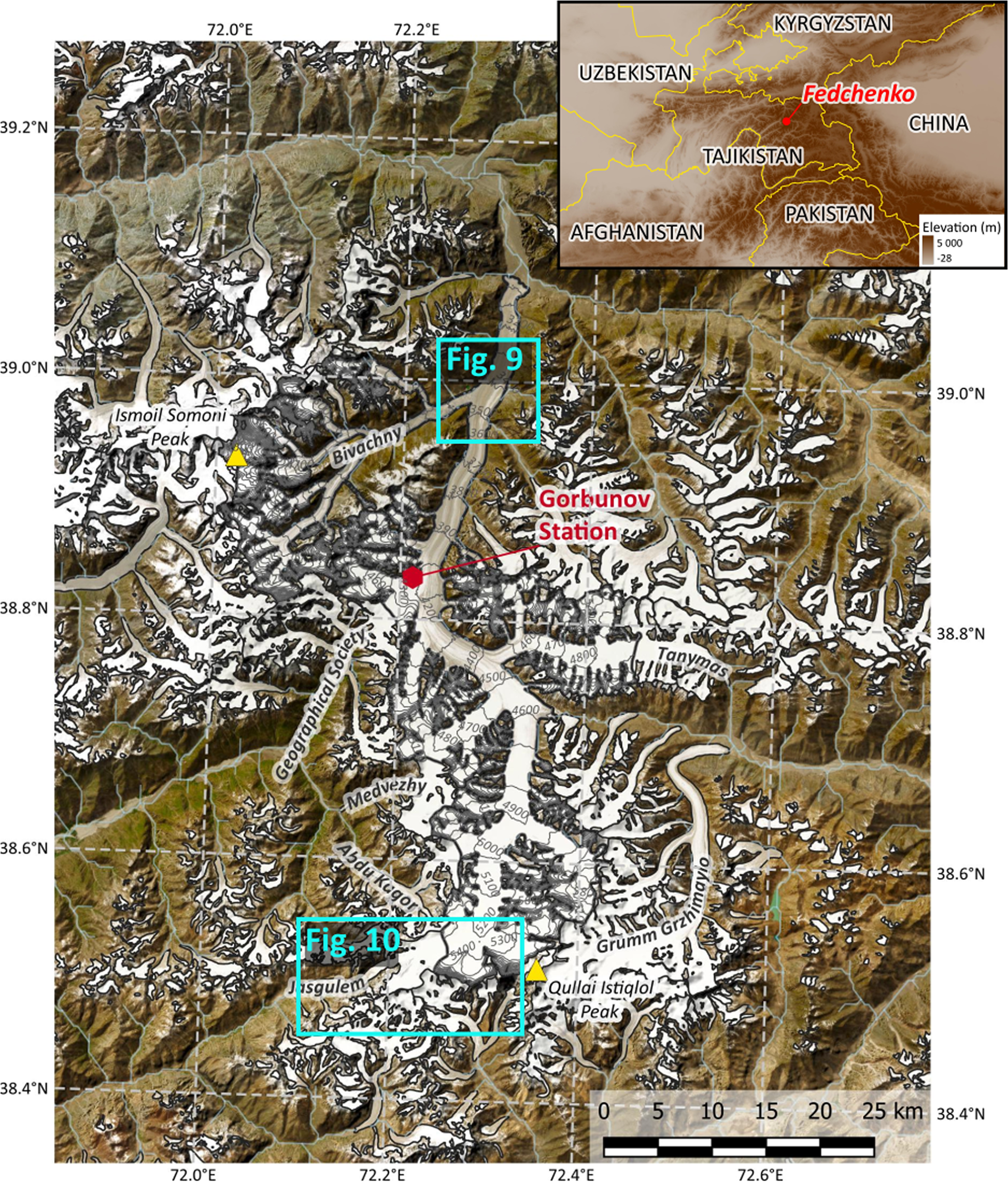
Figure 1. Map of Fedchenko Glacier and surrounding area. Some of the large neighboring glaciers are named on the map. The location of Gorbunov meteorological station is highlighted, as well as the confluence with Bivachny Glacier and Jasgulem pass that are also shown in Figures 9 and 10. Background image is the ESRI satellite product. The inset shows the location of Fedchenko Glacier within Central Asia. Elevation is shown in brown shades, but the scale is truncated at 5000 m a.s.l.
Fedchenko Glacier is located in a region that is known for its very high concentration of surge type glaciers (Sevestre and Benn, Reference Sevestre and Benn2015, Goerlich and others, Reference Goerlich, Bolch and Paul2020, Guillet and others, Reference Guillet, King, Lv, Ghuffar, Benn, Quincey and Bolch2022, Guo and others, Reference Guo, Li, Dehecq, Li, Li and Zhu2023). It has multiple tributary glaciers of various sizes, with Bivachny Glacier being one of the most remarkable, known for its numerous past surges in 1976–78, 1991 and 2011–15 (Kotlyakov and others, Reference Kotlyakov, Osipova and Tsvetkov2008, Wendt and others, Reference Wendt, Mayer, Lambrecht and Floricioiu2017). Most neighboring glaciers of Fedchenko Glacier are surge-type glaciers (Kotlyakov and others, Reference Kotlyakov, Osipova and Tsvetkov1997). In particular, Medvezhiy Glacier, located in the Abdu Kagor river basin and sharing a saddle with Fedchenko Glacier, was extensively studied in the field, and its 10–15 year surge cycle is well documented (Dolgushin and Osipova, Reference Dolgushin and Osipova1973, Osipova, Reference Osipova2015, Murodov and others, Reference Murodov, Li, Safarov, Lv, Murodov, Gulakhmadov, Khusrav and Qiu2024). Fedchenko Glacier is not considered as a surge-type glacier in any of the above-mentioned inventories but is categorized as a glacier with individual signs of instabilities (Kotlyakov and others, Reference Kotlyakov, Osipova and Tsvetkov1997).
3. Data and methods
3.1. Elevation data
3.1.1. Historical maps
Historical maps of Fedchenko Glacier were produced following two expeditions in 1928 and 1958 (Finsterwalder and others, Reference Finsterwalder, Nöth, Reinig, Ficker, Rickmers and der Deutschen Wissenschaft1932, Dittrich, Reference Dittrich1964, Lambrecht and others, Reference Lambrecht, Mayer, Aizen, Floricioiu and Surazakov2014) by terrestrial photogrammetry at a scale of 1:50 000. The maps are all based on the same local geodetic system, defined by astronomic measurements during the expedition in 1928. Scans of the original maps have recently been orthorectified according to their original projection (Lambrecht and others, Reference Lambrecht, Mayer, Aizen, Floricioiu and Surazakov2014). The map contours have intervals of 25 m and 12.5 m on flat areas and were digitized and interpolated by kriging on a regular grid with a resolution of 20 m by 20 m (Lambrecht and others, Reference Lambrecht, Mayer, Aizen, Floricioiu and Surazakov2014). The errors of the final gridded elevation models were previously estimated to less than 35 m in location and about 10 m in elevation (Lambrecht and others, Reference Lambrecht, Mayer, Aizen, Floricioiu and Surazakov2014). We used the maps only along the center line of Fedchenko Glacier in order to avoid challenging areas, such as steep slopes. Further details about the map coverages and DEM generation can be found in Lambrecht and others Reference Lambrecht, Mayer, Aizen, Floricioiu and Surazakov(2014).
3.1.2. DEMs from optical satellite images
We use DEMs from different types of optical images that were all processed without ground control points (Table 1). All the elevation data are posted in the UTM 43N coordinate system and the elevations are provided relative to the WGS84 ellipsoid.
Table 1. Summary of gridded elevation data used in this study
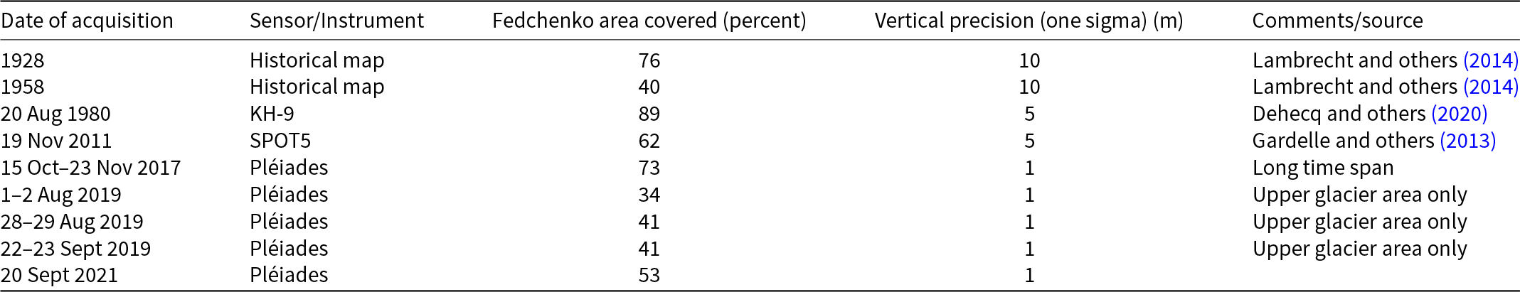
A pair of declassified KH-9 Hexagon images acquired on 20 August 1980 over the Pamir region was selected. This image pair is different from the image of 13 July 1975 used by Zhou and others Reference Zhou, Li, Li, Zhao and Ding(2019). We chose the 1980 images because it was acquired closer to the end of the ablation season, and hence was more favorable to study glacier elevation changes. Additionally, the 1980 images are less saturated in the accumulation basin of Fedchenko Glacier, leading to the reconstruction of a larger area compared to the images of 1975. The images were processed following Dehecq and others Reference Dehecq(2020).
Also, the SPOT 5 HRS DEM from Gardelle and others Reference Gardelle, Berthier, Arnaud and Kääb(2013) was included in the study. This DEM was produced by the French Mapping Agency (IGN) using correlation parameters defined during the SPIRIT (SPOT 5 stereoscopic survey of Polar Ice: Reference Images and Topographies) International Polar Year project (Korona and others, Reference Korona, Berthier, Bernard, Rémy and Thouvenot2009). We used the DEM derived with the second set of parameters (v2), that is in principle better suited for mountainous terrain (Korona and others, Reference Korona, Berthier, Bernard, Rémy and Thouvenot2009, Gardelle and others, Reference Gardelle, Berthier, Arnaud and Kääb2013). Pixels with a correlation score below 75 were excluded, leading to large data voids in the accumulation area (Fig. A1). Finally, we converted the elevation provided with the Earth Gravitational Model 1996 geoid (EGM96) as reference to the WGS84 ellipsoid using the dem_geoid command of NASA’s Ames Stereo Pipelines (ASP, Beyer and others, Reference Beyer, Alexandrov and McMichael2018).
In addition, we use five Pléiades DEMs from 2017, 2019 and 2021 (Table 1). The acquisitions of 2019 are restricted to the upper basin, and the acquisition of 2017 does not cover the lowermost section of the tongue (Fig. A1). Apart from the images of early August 2019, the images are not saturated thanks to the 12-bit encoding and the specific acquisition parameters (Berthier and others, Reference Berthier2024). The pairs of images were processed using ASP. We used a semiglobal matching algorithm, which proved appropriate for snow covered areas (Deschamps-Berger and others, Reference Deschamps-Berger, Gascoin, Berthier, Deems, Gutmann, Dehecq, Shean and Dumont2020). Each Pléiades DEM in Table 1 was obtained by stitching up to three DEMs corresponding to the respective individual Pléiades pairs needed to cover the whole glacier area. In 2019, for a given date, all the scenes were acquired within 2 days, ensuring very limited terrain changes, even over glacierized area. In 2017, the different scenes were acquired more than 1 month apart (15 October–23 November). However, there was limited snowfall between the different acquisitions (i.e. no change in the surface cover) and melt is assumed to be negligible at that time of the year, we assume that changes in elevation are likely minor even on the glacierized area. Thus, stitching was done by co-registering the different DEMs of 2017 using a Nuth and Kääb Reference Nuth and Kääb(2011) co-registration algorithm that considers the entire area covered by the DEMs (and not only the off glacier terrain).
3.1.3. ICESat data
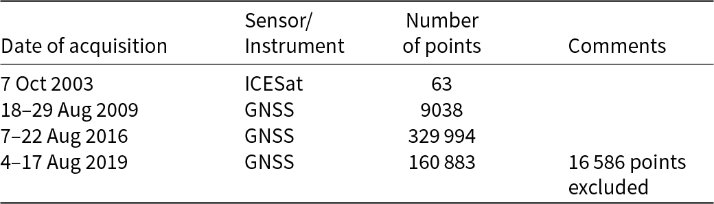
Over the whole ICESat record, there is only one track that intersected Fedchenko Glacier in fall 2003 (Fig. A2). ICESat footprints from the Geoscientific LASer instrument (GLAS) were converted from the EGM2008 geoid to the WGS84 ellipsoid using the NSIDC GLAS Altimetry elevation extractor Tool (NGAT). The nominal precision of ICESat is estimated around 0.1 m on flat terrain (Zwally and others, Reference Zwally2002). We averaged the elevation of the Pléiades 2021 DEM in disks of 70 m diameter around the ICESat footprint center-point and excluded the footprints with a standard deviation of elevation larger than 2 m that corresponds to slopes steeper than ∼10∘. After filtering, we kept 63 footprints that were all acquired on 7 October 2003 (Table 2 and Fig. A2).
Table 2. Summary of point scale data used in this study
3.1.4. GNSS data
GNSS data were gathered during the summers of 2009, 2016 and 2019, employing various GNSS systems. Initially, only GPS and GLONASS were utilized, but with the advancement of Galileo, it was integrated into the 2019 campaign. All measurements were conducted using multi-frequency systems to optimize GNSS signal utilization. The antenna was mounted on a sledge, maintaining a constant height above the surface. In 2009, the analysis relied on a local GNSS reference station on the glacier, whose coordinates were estimated using data from the nearest International GNSS Service (IGS) site. The sledge’s coordinates were then computed relative to this local reference station. After 2009, precise point positioning became the method for position estimation, relying on precise clock and orbit data from GNSS satellites. This approach eliminates the need for a local reference station, simplifies fieldwork as there is no setup or maintenance required for power supply. GNSS campaigns of 2009 and 2016 are described in Lambrecht and others Reference Lambrecht, Mayer, Wendt, Floricioiu and Völksen(2018). The GNSS campaign of 2019 was primary designed to provide an absolute co-registration to the Pléiades DEM of 2019, which was tasked simultaneously to the field campaign. In order to ensure robust constrains on the horizontal co-registration of the Pléiades DEM, we covered terrain with various slopes and aspects with the GNSS (Fig. A3).
The accuracy of each position is better than 10 cm in the horizontal components and 20 cm in height, which is still a conservative estimate (Lambrecht and others, Reference Lambrecht, Mayer, Wendt, Floricioiu and Völksen2018). Coordinates were determined within the International Terrestrial Reference Frame (ITRF). In the first two campaigns, coordinates were referenced to ITRF2008, while the last campaign used the ITRF2014, introduced shortly before. Both reference frames exhibit negligible differences with a typical magnitude of 1 cm, which is much lower than other sources of uncertainties. The current realizations of WGS84 and various ITRFs differ in the centimeter range, as they only differ in the continuous improvement of the data used, the modeling of geophysical phenomena and the consideration of long-term measurements. However, for our practical purposes, we consider them to be identical and will summarize both under the term WGS84 in the following sections.
3.2. Elevation change methods
3.2.1. Co-registration
All the elevation data (i.e. GNSS and DEMs) are converted to the same spatial reference system (WGS84) and projected into UTM coordinates (43N) using ellipsoidal heights. For the DEMs derived from historical maps of 1928 and 1958, Lambrecht and others Reference Lambrecht, Mayer, Aizen, Floricioiu and Surazakov(2014) ensured the consistency between the original astronomical system and the WGS84 ellipsoidal elevation, which includes correcting the map elevations by a 32 m offset. This offset agrees well with the geoid height provided by the EGM96. Details regarding the processing of the maps are available in Lambrecht and others Reference Lambrecht, Mayer, Aizen, Floricioiu and Surazakov(2014) and in references therein. The location error was estimated around 35 m, and due to the limited stable terrain available, we did not apply another co-registration (Lambrecht and others, Reference Lambrecht, Mayer, Aizen, Floricioiu and Surazakov2014). The DEMs from optical satellite data, calculated from orbital parameters, are not perfectly georeferenced. For each of them, the horizontal and vertical georeferencing can have an offset of up to dozen of meters. As a consequence, they need to be tied to the GNSS data before being differentiated.
We first co-registered the 1–2 August 2019 Pléiades DEM on the GNSS data acquired just a few days later on 4–17 August 2019. Due to the insufficient variety of slope and aspect, automatic algorithms did not perform well. Instead, we manually found the horizontal displacement (x and y direction) that minimized the typical aspect dependent pattern of horizontally shifted elevation products (Berthier and others, Reference Berthier, Arnaud, Kumar, Ahmad, Wagnon and Chevallier2007, Nuth and Kääb, Reference Nuth and Kääb2011). The standard deviation of the difference between the Pléiades DEM and the GNSS points is 0.41 m after excluding one spurious series of GNSS measurements (Fig. A3). We then co-registered the Pléiades DEM of 2019 and 2021 on the mosaic of 1–2 August 2019 DEM using a classical co-registration algorithm (Nuth and Kääb, Reference Nuth and Kääb2011). As the August 2019 Pléiades acquisition targeted the glaciers’ upper accumulation area, they contain very limited stable terrain, which make them unsuitable to co-register lower precision DEMs. Instead, the 2021 Pléiades DEM covers a larger terrain and is thus used as a reference to co-register the remaining Pléiades, KH-9 and SPOT5 DEMs. In summary, we co-registered the 2019 DEM on the 2019 GNSS, then the 2021 DEM on the 2019 DEM and finally, all the other DEMs on the 2021 DEM. The values of the shifts are summarized in Table A1.
3.2.2. Analyzing spatially discontinuous elevation changes
One of the challenges of studying the elevation changes of a glacier that has the size of Fedchenko glacier is the difficulty to obtain precise elevation data that cover the whole glacier area. In particular, the GNSS measurements were acquired along individual profiles, and even if there are some cross overs between profiles in the different years, they provide only localized elevation changes. In order to combine elevation information from different spatial sampling, we apply a method inspired from ICESat processing (Kääb and others, Reference Kääb, Berthier, Nuth, Gardelle and Arnaud2012). We create a 700 m wide buffer along the glacier center line, which we split into 1 km long sections along the main glacier flow, these sections are called patches hereafter (Fig. 4). We difference all the available elevation data (DEM and GNSS) with regard to the Pléiades 2021 DEM. GNSS data are differentiated with the Pléiades 2021 DEM using the Point sampling tool in QGIS. ICESat data are differentiated with the average elevation of the Pléiades 2021 DEM in disks of 70 m diameter around the footprint center-point.
For each patch and for each year i, we calculate the average elevation change relative to the 2021 DEM for each period ( $\overline{dh_{i-2021}}$). For the discrete measurements (ICESat and GNSS), we do not apply any filtering. For the continuous measurements (DEMs), we consider as valid the patches with more than 40% of data coverage. For each sub-period between the years i and j, we calculate the elevation change ( $\overline{dh_{i-j}}$) as:
 \begin{equation}
\overline{dh_{i-j}} = \overline{dh_{i-2021}} - \overline{dh_{j-2021}}
\end{equation}
\begin{equation}
\overline{dh_{i-j}} = \overline{dh_{i-2021}} - \overline{dh_{j-2021}}
\end{equation}using 2021 as the general reference level.
3.3. Uncertainties on elevation changes
Uncertainties on elevation changes are very difficult to quantify due to the heterogeneous sources of data and the spatial averaging done here. The main sources of uncertainties on elevation changes are (i) the intrinsic precision of the data, (ii) the spatial sampling and (iii) the temporal sampling.
3.3.1. Intrinsic precision of the data
Due to the limited stable terrain and the contrast between the rugged stable terrain and gentle glacier terrain, we cannot apply standard methods to evaluate the spatial structure of variance (e.g. Rolstad and others, Reference Rolstad, Haug and Denby2009, Hugonnet and others, Reference Hugonnet, Brun, Berthier, Dehecq, Mannerfelt, Eckert and Farinotti2022). Instead, we report only one single metric of DEM precision, based on the literature (Table 1). We do not account for the effect of spatial averaging for DEM differences because we investigate patches that are expected to be small with respect to the decorrelation length of the DEM differences. At the scale of the patch, the errors are thus highly correlated. However, when looking at a collection of patches, the spatial correlation reduces due to the distance between patches.
3.3.2. Spatial sampling
For the point-scale measurements (GNSS and ICESat), we need to test whether the measured elevation changes are representative of the patch they belong to. To assess the impact of the spatial sampling, we sampled the Pléiades 2017 and 2021 DEMs at the locations of each GNSS point and ICESat footprint. For each patch, we average the elevation differences obtained with the GNSS or ICESat sampling and compare it with the 2017–21 DEM difference averaged over the same patch. We find that the GNSS sampling is very representative for both campaigns, with a mean difference of 0.00 m (std of 0.28 m) for the 2009 GNSS campaign and 0.05 m (std of 0.34 m) for the 2016 GNSS campaign. For ICEsat, we find lower accuracy with a mean difference of −0.17 m and a standard deviation of 0.54 m. The difference is likely due to the fact that the ICESat track intersects the side of the glacier, while the GNSS tracks follow the center line (Fig A2).
3.3.3. Temporal sampling—Seasonal correction of the GNSS elevations
The GNSS data were acquired around mid-August (Table 2). These dates are not ideal to calculate elevation changes, which should preferentially be calculated between matching dates at the end of the ablation season (i.e. 1 October). The sub-annual acquisitions of Pléiades data in 1–2 August, 28–29 August and 22–23 September 2019 were used to derive a correction (in m) that was applied to the GNSS data of 2009 and 2016 (Fig. A4). The correction is calculated as the difference between the end of September DEM minus the average of the two DEMs acquired in August, which is a proxy for a mid-August DEM. This seasonal correction is available only for the upper part of the glacier, above 4500 m. It averages at −0.66 m, can be as negative as −1.53 m and has generally a higher magnitude for lower elevations, with the exception of the highest locations that experienced a thinning of 0.90 m.
We applied the seasonal correction to GNSS data only, because the ICESat data were acquired very close to the target date of 1 October (Table 2). Regarding the DEMs, only one was acquired more than 1 month before the end of the ablation season (the KH-9 DEM of 20 Aug 1980), but we did not apply a correction as it would have a small impact on yearly change rates due to the long time spans considered.
3.4. Meteorological data
Meteorological data originate from two sources: the Gorbunov/Fedchenko Station (Williams and Konovalov, Reference Williams and Konovalov2008) located at 4169 m on the eastern side of the glacier and ERA5 reanalysis data (Hersbach and others, Reference Hersbach2020). We use monthly values of temperature and precipitation from both sources. We also use monthly snowfall from ERA5 reanalysis data, in order to discriminate solid and liquid precipitation. Fedchenko Station operated from 1936 to 1994, providing an exceptional climate record in this data scarce and remote area, even though one should keep in mind that the measurement of precipitation in mountainous environment is challenging and prone to under-catch (e.g.
Kochendorfer and others, Reference Kochendorfer2017). ERA5 reanalysis was recently extended back to 1950, which leads to an overlap of 44 years between the two records. We collected ERA5 series of temperature, precipitation and snowfall from the closest grid point to the station (72.25, 38.75). It has a geopotential height of  $44\,368\,\mathrm{m}^2$ s−2, corresponding to an elevation of 4527 m, assuming g 0 = 9.80 m s−2.
3.5. Meteorological methods
3.5.1. Bias correction in ERA5 data
Due to the height difference between the station and ERA5 grid point and the cold bias in mountainous area in ERA5 (e.g. Orsolini and others, Reference Orsolini2019, Khadka and others, Reference Khadka, Wagnon, Brun, Shrestha, Lejeune and Arnaud2022), we find a temperature bias of −5.9 K in ERA5, relative to the Gorbunov station. After correcting for this bias, we still observe a season dependent bias, with the spring/summer months being positively biased up to 1.6 K in April, and the fall/winter months being negatively biased down to −2.3 K in November (Fig. A5). After removing a monthly bias, the final match between ERA5 monthly temperature and the station monthly temperature is very good, with an RMSE at 1.4 K (Fig. 2a). At annual scales, the agreement between ERA5 and the station is also strong (Fig. 3). For the shared period, the inter annual variability is slightly higher in ERA5 (0.66 K) than in the station data (0.53 K).

Figure 2. Comparison of the monthly ERA5 bias corrected temperature (a) and precipitation (b) with the monthly station record for the overlapping years (1950–94). Note that the years 1990–94 were excluded for the precipitation data, due to spurious values in the station record.
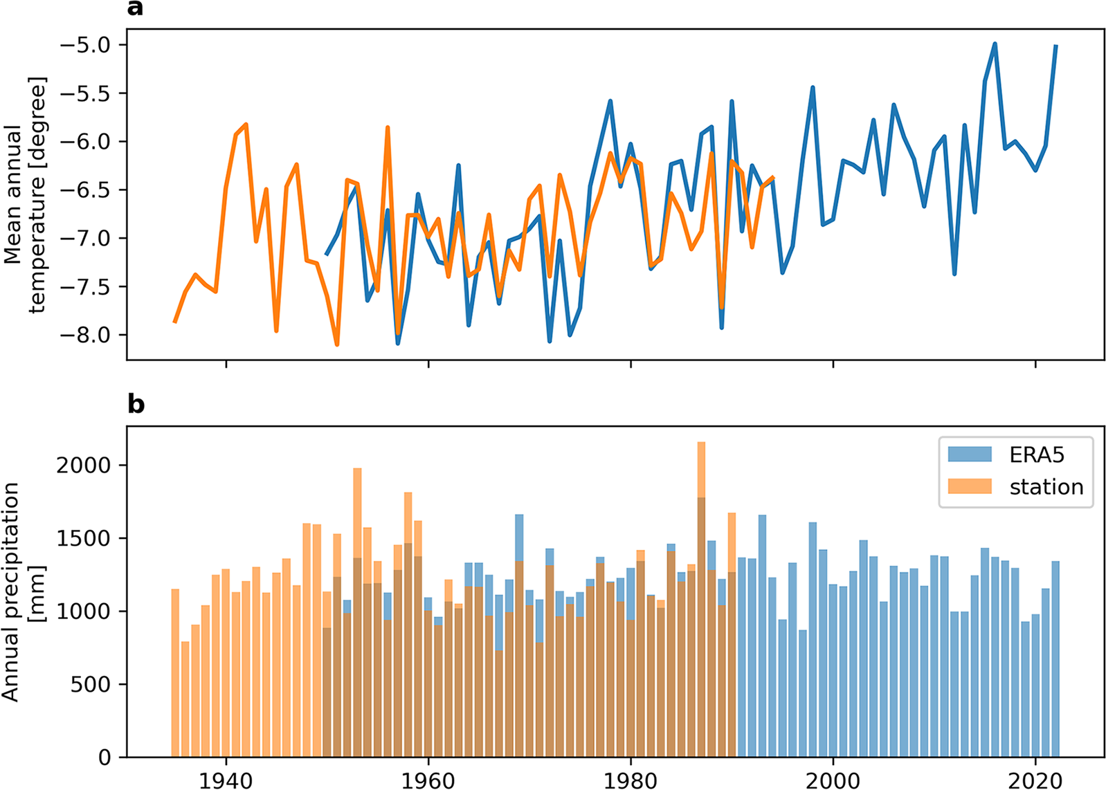
Figure 3. Series of annual temperature (a) and precipitation (b) from ERA5 corrected and from the station record.
There is more dispersion in the difference between ERA5 and the station records for precipitation than for temperature, with a systematic underestimation of precipitation in ERA5. We multiply the ERA5 precipitation by 1.9, which minimize both the RMSE and the bias between the two series (Fig. 2b). The comparison shows an RMSE of 38 mm in the monthly precipitation data, but the bias between the two series is limited, with a mean bias of 1 mm, which ensures that the two series can still be merged (Fig. 3). Note that these statistics are calculated excluding the station data after 1990, because there is a systematic negative bias in the precipitation records (Fig. A6). For the shared period, the station has a higher inter-annual variability (std of 305 mm yr−1) than ERA5 (std of 175 mm yr−1). We apply the same factor of 1.9 to correct ERA5 snowfall.
3.5.2. Temperature and precipitation anomalies
We create two meteorological records named ‘ERA5 priority’ and ‘station priority’, depending on which dataset is used in the shared period. For the reconstructed temperature and precipitation series, the anomalies are calculated on a monthly basis for the whole period (1936 until 2020). For each year, we calculate the anomaly in each variable by subtracting the monthly averages over the whole period to the monthly series. We also calculate annual snowfall anomalies from ERA5 record. Note that the latter are calculated as percentage and are thus unaffected by the precipitation correction factor.
4. Results
4.1. Multi-decadal elevation changes
For the period 1928–2021, the coverage of the glacier with elevation information is high (Table 1), especially along the central flowline that is fully covered. We observe a mean thinning rate of 0.46 m yr−1, with a maximum thinning of 89.4 m (corresponding to 0.96 m yr−1) roughly 4 km from the glacier front around 3100 m a.s.l. (Fig. 4 and Table 3). The thinning is relatively homogeneous for the lower reaches and then decreases with elevation from ∼80 m at 3700 m a.s.l to less than 10 m at 4600 m a.s.l. There is almost no elevation change detectable from 4600 to 5000 m a.s.l. (dh/dt around  $-0.10\,\mathrm{m\ yr}^{-1}$; Figs. 4 and 5), but thinning increases again above 5000 m a.s.l. reaching ∼30 m at Jasgulem pass (5250 m a.s.l.).
For the four sub-periods (1928–58, 1958–80, 1980–2010 and 2010–21), the coverage is not always complete. For the period 1928–58, we limit the analysis to the area below 4900 m a.s.l., because of spurious data above this elevation (Lambrecht and others, Reference Lambrecht, Mayer, Aizen, Floricioiu and Surazakov2014). During this 30 year period, thinning is moderate in the tongue region (−0.31 m yr−1) and close to zero for most of the surveyed area located between 3700 and 4900 m a.s.l. For the period 1958–80, we observe a marked thinning at all elevations, with a maximum thinning of −1.44 m yr−1 around the confluence with Bivachny Glacier. The pattern of elevation change is peculiar, as there is a rather sharp transition toward less negative rates of elevation changes seven kilometers upstream of the confluence with Bivachny Glacier. Significant thinning rates are still observed at all elevations, until the maximum observed elevation of 4900 m a.s.l. For the period 1980–2010, the glacier thinned in the lower parts (−0.68 m yr−1) but slightly thickened in the main trunk from 4700 to 5200 m a.s.l. It is noteworthy that the year 2010 reconstruction is a combination of the SPOT5 DEM of November 2011, for elevations below 4600 m a.s.l. and of the GNSS measurements of August 2009 for the upper parts (Figs. A1 and A2). For the period 2010–21, the thinning is observed at all altitudes, with rates of elevation change around −0.87 m yr−1 for the tongue, and a homogeneous elevation change rate of −0.31 m yr−1 in the whole accumulation area (Fig. 4).
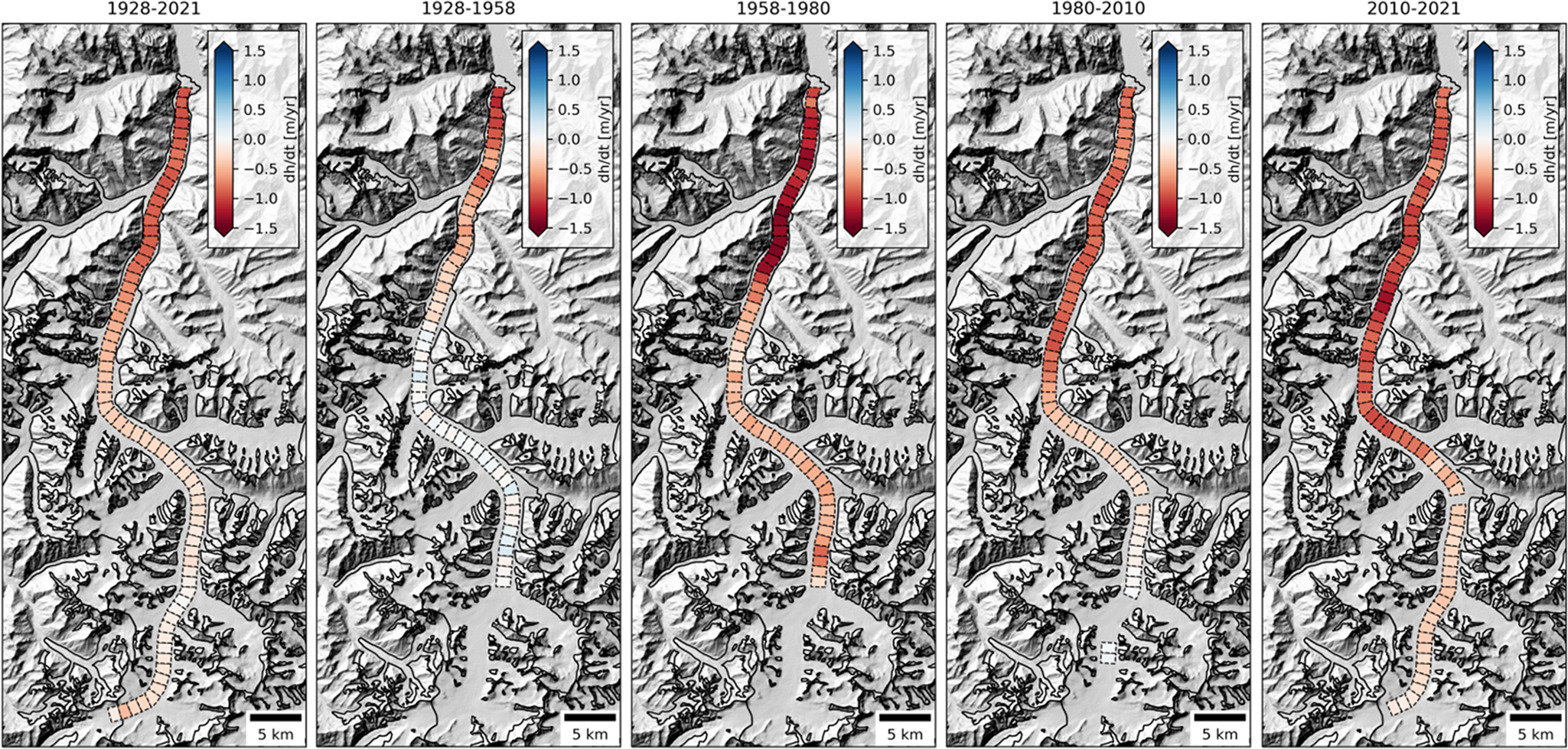
Figure 4. Rates of elevation changes along the main trunk of Fedchenko Glacier for the different sub-periods. Background is a hillshade from the Copernicus 30 m DEM (GLO-30DEM; European Space Agency, 2022). Note that elevation changes are spatially averaged on the patches as described in the method section.
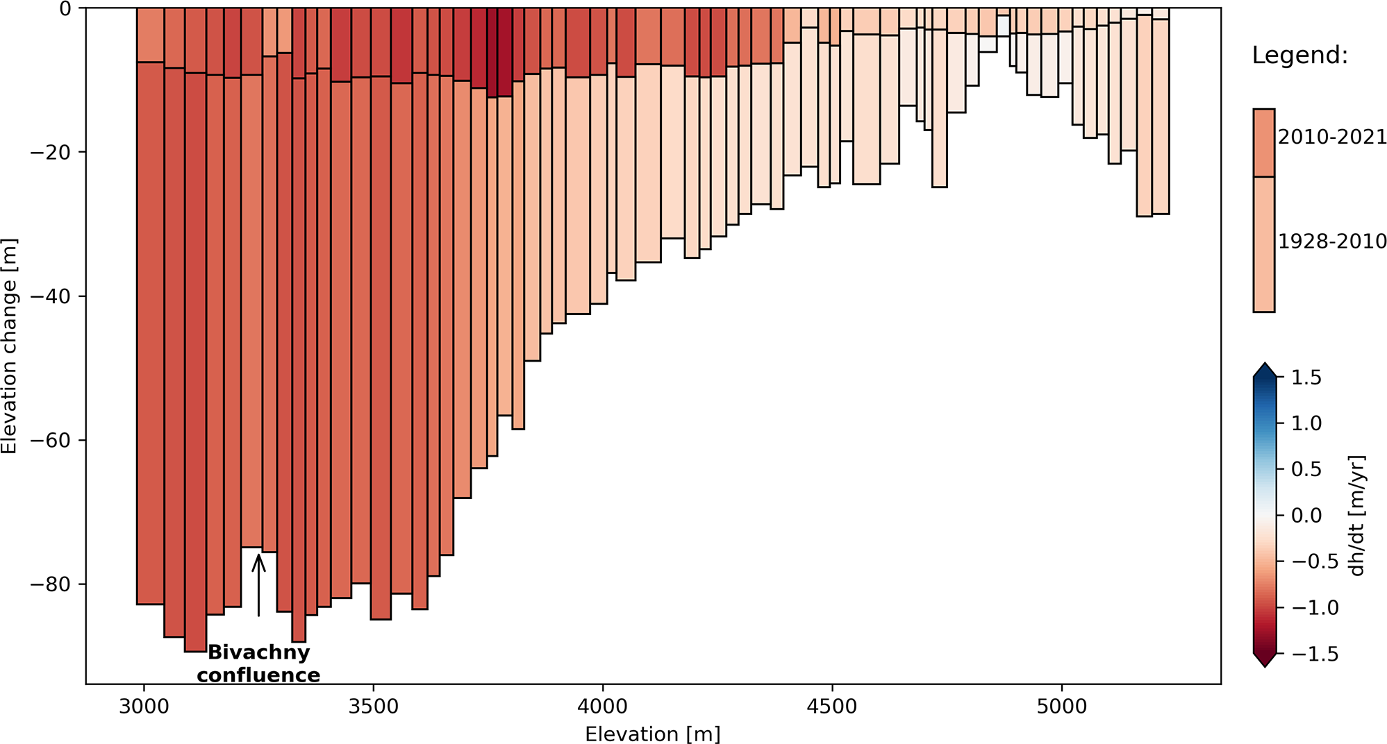
Figure 5. Elevation changes for the periods 1928–2010 and 2010–21 for different elevations along the center line of Fedchenko Glacier. The bar length represents the elevation change and their color the rate of elevation change. The bar width represents the altitudinal span of each patch. The arrow shows the location of the confluence with Bivachny Glacier and the reduced thinning due to the surge of Bivachny (Wendt and others, Reference Wendt, Mayer, Lambrecht and Floricioiu2017).
Table 3. Rate of elevation changes for the different sub-periods. The ‘whole area’ corresponds to the average of all the patches with elevation change rate values and can be thus heavily biased when the sampling is not optimal. The ‘shared area’ corresponds to locations that are sampled during all sub-periods and is thus restricted to lower reaches of the glacier. The ‘upper area’ corresponds to elevations above 4600 m a.s.l. and the ‘lower area’ corresponds to elevations below 4600 m a.s.l.. For some periods, the upper area is very poorly sampled and the mean elevation change is not very meaningful, these values are marked with a star ( $^*$)
$^*$)
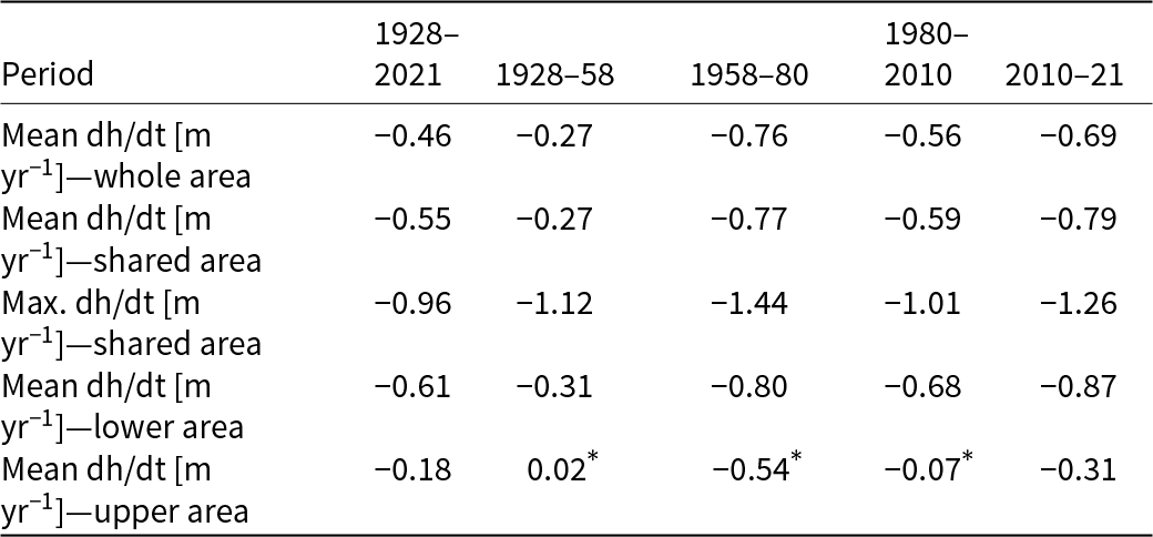
In order to compare the different sub-periods in a more quantitative way, we calculate the mean rate of elevation change over the area covered in all the sub-periods (see ‘shared area’ in Table 3). We find an elevation change rate of −0.55 m yr−1 for the period 1928–2021. The period with the most limited changes is 1928–58, with a rate of -0.27 m yr−1, while the period 1980–2010 is close to the long term average with −0.59 m yr−1. The two sub-periods 1958–80 and 2010–21 are the most negative ones with rates of elevation changes of −0.77 and −0.79 m yr−1, respectively.
If we compare the most recent period (2010–21) with the earlier 82 years (1928–2010), the most striking feature is the up-glacier propagation of substantial thinning rates ( $ \gt 1\ \mathrm{m\ yr}^{-1}$) at elevations above 3700 m a.s.l. (Fig. 5). In contrast, the thinning rates of the lowest parts of the glacier are very similar and average at −0.90 m yr−1 below 3600 m a.s.l. for both periods. We find opposite results at the upper most elevations (above 5200 m a.s.l. at Jasgulem pass), where the early thinning rate of −0.32 m yr−1 is larger than the contemporary one at −0.13 m yr−1.
4.2. 2003–21 elevation changes
Short-term elevation changes are available only for the accumulation basin and are based on ICESat, GNSS data and Pléiades DEMs (Fig. 6). The 2003–09 period coverage is limited, because it is based on a single ICESat track from 7 October 2003, despite a good coverage from the GNSS in 2009 (Fig. A2). It is also noteworthy that ICESat sampling represents the spatial variability with less accuracy (see Section 3). Still, we observe significant thinning, ranging from −0.57 to −0.28 m yr−1 in the upper accumulation basin from 2003 to 2009, followed by a period (2009–16) of more moderate thinning, that averages at −0.21 m yr−1. The last period (2016–2021) is the most spatially contrasted, with areas of strong thinning (−0.82 m yr−1) and areas of thickening up to 0.16 m yr−1 (Fig. 6).
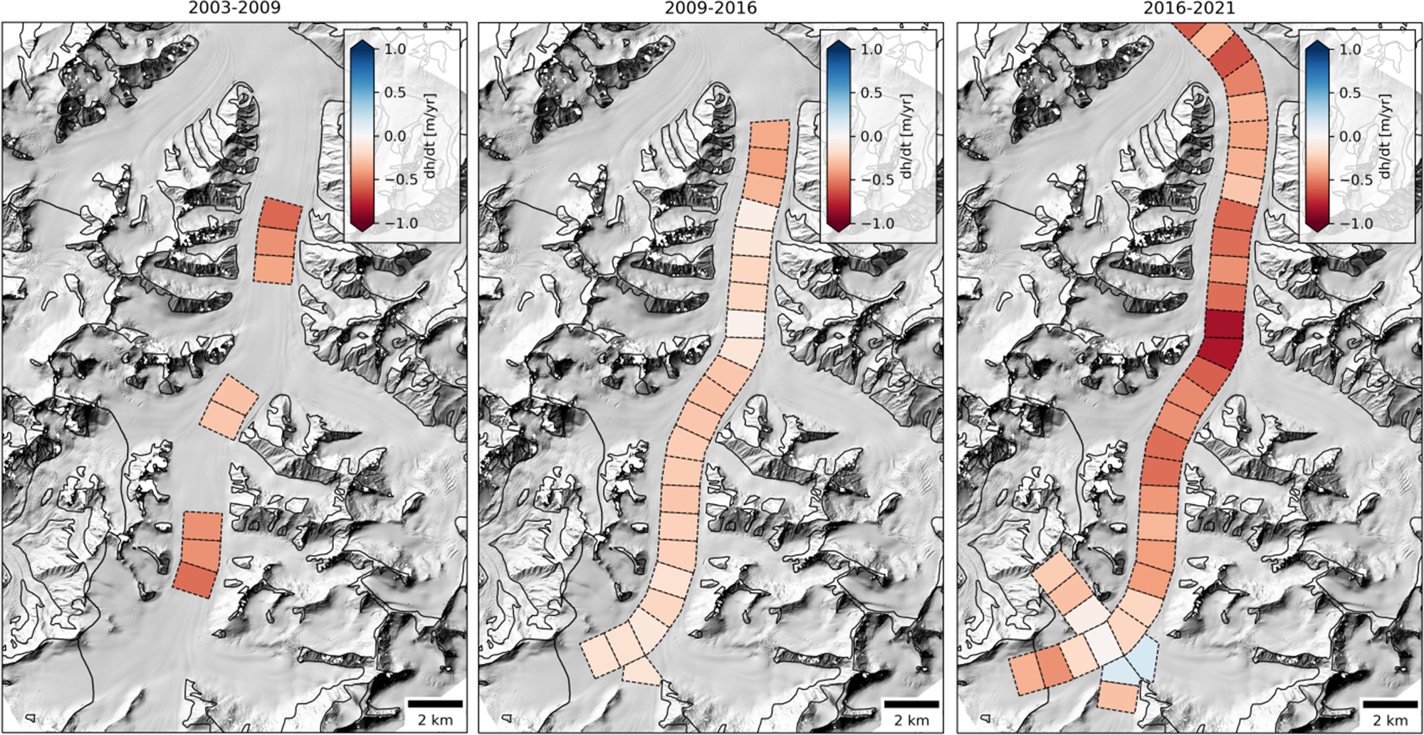
Figure 6. Rates of elevation changes for three sub-periods in the higher part of Fedchenko Glacier from 2003 to 2021.
It is difficult to compare the three sub-periods, because of the limited spatial coverage for 2003–09. However, the mean rate of elevation change is roughly twice as negative for the period 2016–21, than for the period 2009–16, with mean rates of elevation changes of −0.41 and −0.21 m yr−1, respectively. The localized thickening pattern for the period 2016–19 is a robust pattern, also visible in the 2015 GNSS data (not shown here, because the coverage is scarce). There is little dependency of the elevation change with elevation. For instance, the maximum thinning rate for the period 2016–21 is located at 4900 m a.s.l. For the period 2009–2016, the rate of elevation change is slightly higher for the lower elevations, but differences are still rather small.
Overall, the accumulation basin of Fedchenko Glacier has thinned at a substantial rate since 2000, but it is difficult to quantify the magnitude of these changes and their acceleration. The recent rates of elevation changes (2010–21) are more negative than the long term trend (1928–2010), with the exception of Jasgulem pass, where most of the changes happened before 2010.
4.3. Meteorological changes
Both reconstructed time series show a continuous increase in temperature (Fig. 7), reaching an annual temperature anomaly of 0.60 K for the period 2010–21, with respect to the period 1936–2021. Regarding precipitation, the year-to-year variability is large (Fig. 7). In both reconstructed records, there is a positive precipitation anomaly from 1980 to 2010 of 5–7%. Additionally, in the ‘station priority’ record, the period 1958–80 corresponds to a dry anomaly, with a 10% precipitation deficit, but this is not visible in the ‘ERA5 priority’ record, which shows only a moderately negative precipitation anomaly for this period (Fig. 7). The snowfall at ERA5 grid point has a marked positive anomaly of 6 % for the period 1980–2010 and a very negative anomaly of −12% for the period 2011–21, which is likely related to the positive temperature anomaly and might not be representative of what happens at higher elevation (Fig. 8).
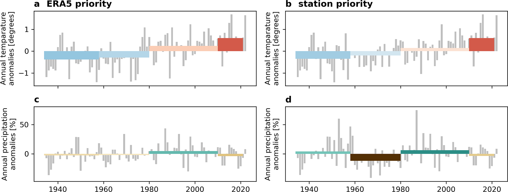
Figure 7. Anomalies of temperature (a, b) and precipitation (c, d) for the ‘ERA5 priority’ (a, c) and ‘station priority’ (b, d) records. Colored boxes show the period considered in this study bounded by elevation data availability.
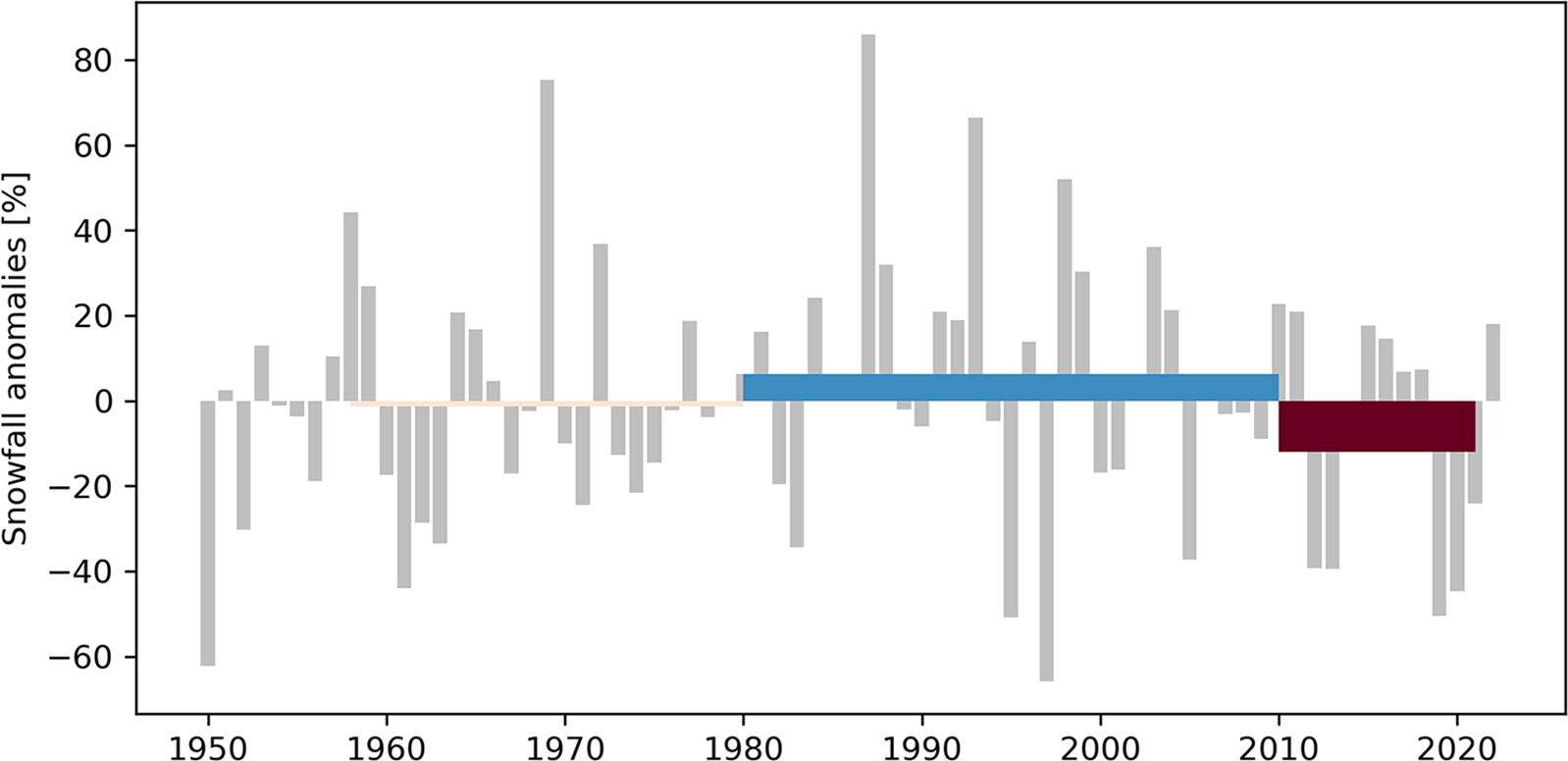
Figure 8. Annual snowfall anomalies from ERA5 record.
5. Discussion
5.1. Climate-related elevation changes
Long-term elevation changes of Fedchenko Glacier are not homogeneous in time. While it is rather clear that the glacier has been thinning for almost a century (Lambrecht and others, Reference Lambrecht, Mayer, Aizen, Floricioiu and Surazakov2014), our study allows to identify different patterns and rates of elevation changes for each sub-period that deciphers a complex glacier/climate relationship.
The earliest period is the one with the most limited changes of the glacier (from the terminus to 4600 m elevation), with an average thinning of −0.27 m yr−1 (Table 3). The thinning is still significant, as well as the tongue retreat, showing that the glacier was already out of equilibrium with climate. The limited data collected above 4600 m a.s.l show near zero elevation changes, meaning that the surface mass balance was in equilibrium with the dynamics in the upper part of the glacier. This hints toward a slight disequilibrium with climate, that could be an ongoing response of Fedchenko Glacier to the end of the little ice age, which is estimated to culminate around 1600–50 years AD in the Pamir Alay (Solomina, Reference Solomina2000).
A period of intense thinning between 1958 and 1975 for the glacier tongue was suspected by Zhou and others Reference Zhou, Li, Li, Zhao and Ding(2019), because they found lower thinning rates for the period 1975–2000 than Lambrecht and others Reference Lambrecht, Mayer, Aizen, Floricioiu and Surazakov(2014) for the period 1958–2000. Our study confirms their interpretation, as we find a mean rate of elevation change of −0.77 m yr−1 over the shared area for the period 1958–80. In terms of climatic record, the station data show rather dry conditions (anomaly of −10%) during this period (Fig. 7); however, this is not reflected in the ERA5 record (Fig. 7). The period 1968–80 corresponds to negative (−0.52 ± 0.14 m w.e. a−1) mass balance for Abramov Glacier located in the Pamir Alay, 90 km north of Fedchenko Glacier front (Barandun and others, Reference Barandun2015, Kronenberg and others, Reference Kronenberg, van Pelt, Machguth, Fiddes, Hoelzle and Pertziger2022), and the period 1967–73 corresponds to slight mass losses in Muztag Ata Massif (Bhattacharya and others, Reference Bhattacharya2021), which indicates that mass-balance conditions in the region were unfavorable during this time. Thinning in the upper area also suggests dry conditions. Still, the pattern of thinning of the tongue for the period 1958–80 is difficult to explain by a climatic signal only (see Section 5).
The period 1980–2010 corresponds to moderate thinning and even some slight thickening in the upper area of Fedchenko Glacier (Table 3 and Fig. 4). Moderate glacier mass losses and slight mass gains can be interpreted within the general picture of the ‘Karakoram anomaly’ (Gardelle and others, Reference Gardelle, Berthier and Arnaud2012, Farinotti and others, Reference Farinotti, Immerzeel, de Kok, Quincey and Dehecq2020). This anomaly of positive glacier mass balance is quite well documented for the eastern Pamir in the beginning of the 21st century (Holzer and others, Reference Holzer, Vijay, Yao, Xu, Buchroithner and Bolch2015, Brun and others, Reference Brun, Berthier, Wagnon, Kääb and Treichler2017, Lin and others, Reference Lin, Li, Cuo, Hooper and Ye2017, Zhu and others, Reference Zhu2018, Shean and others, Reference Shean, Bhushan, Montesano, Rounce, Arendt and Osmanoglu2020), but there is no definitive conclusion about its specific drivers (de Kok and others, Reference de Kok, Tuinenburg, Bonekamp and Immerzeel2018, Farinotti and others, Reference Farinotti, Immerzeel, de Kok, Quincey and Dehecq2020). From the ERA5 and station data, it seems that this period corresponds to a wet anomaly (Fig. 7) that led to increased snowfall (Fig. 8). Despite a positive temperature trend and anomaly, the excess precipitation and snowfall might have mitigated the impact of rising temperature, and thus delayed the glaciers’ response to this warming. Moreover, Fedchenko Glacier lies in-between two well-studied glaciers Abramov and Muztag Ata glaciers that are sub-continental and continental types of glaciers, respectively. Fedchenko Glacier is thus expected to be also of continental/sub-continental type with a relatively low sensitivity to temperature changes (Wang and others, Reference Wang, Yi and Sun2017, Reference Wang, Liu, Shangguan, Radić and Zhang2019, Zhu and others, Reference Zhu2018, Arndt and Schneider, Reference Arndt and Schneider2023).
The last period (2010–2021) is the period of most intense thinning, with a mean elevation change rate of −0.79 m yr−1. This is consistent with the largest positive temperature anomaly and the slightly negative precipitation anomaly that led to a large snowfall deficit (Fig. 8). The thinning is widespread, including in the upper area of the glacier, where it reaches −0.31 m yr−1, a number in agreement with previous studies (Lambrecht and others, Reference Lambrecht, Mayer, Wendt, Floricioiu and Völksen2018). The most striking feature is the up-glacier propagation of thinning (Fig. 5). It is noteworthy that this 11 year period is shorter than the other ones, leading to large uncertainties on the rates of elevation changes. The intense thinning is consistent with the accelerating mass losses in high mountain Asia and the possible end of the ‘Karakoram anomaly’ (Bhattacharya and others, Reference Bhattacharya2021, Hugonnet and others, Reference Hugonnet2021). The large snowfall anomaly of −12% for the period 2011–21 shows that there is also an impact of the rising rain-snow transition, because the snowfall anomaly has a larger amplitude than the precipitation anomaly. The most recent thinning is thus likely a combination of intensified melt and reduced accumulation, due to both a lack of precipitation and reduced proportion of snowfall.
5.2. A potential surge on Fedchenko main tongue?
For the period 1958–80, reduced precipitation should lead to generalized thinning, whereas the most intense thinning happens only at the glacier tongue on the lowest 18 km (Fig. 4). Within 2 km, the rates of thinning change from −0.8 to −1.3 m yr−1. Such a pattern suggests the implication of ice dynamics as well and potentially surge-related mechanisms. Large thinning rates localized on glacier tongues are frequently interpreted as post surge phases, but this criterion is not sufficient to classify a glacier as surge-type (e.g. Sevestre and Benn, Reference Sevestre and Benn2015, Goerlich and others, Reference Goerlich, Bolch and Paul2020, and references therein). We thus searched for additional evidence to support or to refute this interpretation.
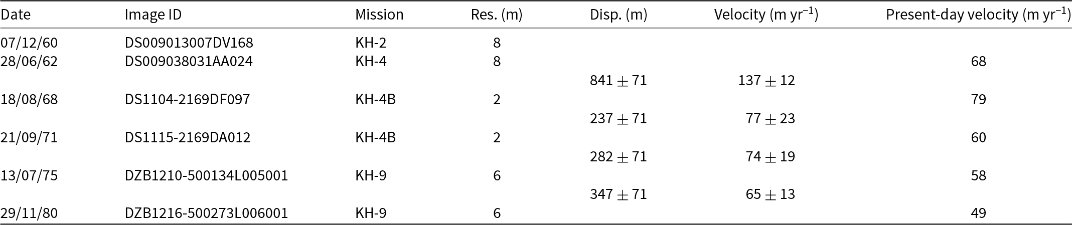
We investigated images from the Corona KH-2, KH-4, KH-4B and Hexagon KH-9 missions that were acquired over the Pamir from the 1960s and 1980s (Zhou and others, Reference Zhou, Li, Li, Zhao and Ding2019, Goerlich and others, Reference Goerlich, Bolch and Paul2020, Ghuffar and others, Reference Ghuffar, Bolch, Rupnik and Bhattacharya2022, Table 4). The orthoimage of 1968 is from Ghuffar and others Reference Ghuffar, Bolch, Rupnik and Bhattacharya(2022), and the orthoimages of 1975 and 1980 are processed according to Dehecq and others Reference Dehecq(2020). The other images are referenced using stable terrain features identified in the Pléiades orthoimage of 2021 and using the georeferencer tool of QGIS. These images are thus not properly orthorectified but simply registered. We used five to seven tie points identified in the Pléiades orthoimage from September 2021 and located on both sides of Fedchenko main tongue to register each image. As a consequence, we assume a positioning uncertainty of 50 m, which is much larger than the resolution of the images and is a conservative estimate (Table 4).
Table 4. KH-2, KH-4 and KH-9 images used to track the looped-moraine displacement. Res. stands for approximative best ground resolution of the image in m. The values in between two rows represent the displacement of the tip of the looped-moraine and derived velocity between the two consecutive scenes. The present-day velocity is the velocity for 2017–18 at the tip of the looped-moraine location extracted from Millan and others Reference Millan, Mouginot, Rabatel and Morlighem(2022). Figure A7 shows the locations of the tip of the looped-moraine for the different dates
Visual inspection of the images reveals that downstream of the confluence with Bivachny Glacier, the central part of Fedchenko tongue was much more crevassed in December 1960, than in the other years, where it appears covered by debris, with distinct ice cliffs. Additionally, on its right side, Fedchenko Glacier is touching the valley walls in December 1960 whereas the ice is ∼100 m away from a deposited moraine in August 1968 (Fig. 9). This observation suggests that parts of the thinning happened at the beginning of the 1958–80 period. This interpretation is in line with the results form Zhou and others Reference Zhou, Li, Li, Zhao and Ding(2019), who observed moderate thinning after 1975.
On the historical images, we also find the existence of a looped moraine on Fedchenko main trunk, located close to the confluence with Bivachny Glacier in 1960 (Fig. 9). Looped moraines are common features related to ice flow instabilities (Meier and Post, Reference Meier and Post1969, Post, Reference Post1972, Jennings and Hambrey, Reference Jennings and Hambrey2021). As the looped moraine is preserved over two decades, we could track its location on the historical imagery (Figs. 9 and A7 and Table 4). We assumed an uncertainty of 50 m on the location of the tip of the looped moraine, which is likely a conservative estimate, especially for the most resolved images. The uncertainty in the displacement in between two images is thus  $\sqrt{2}*50$ = 71 m, leading to uncertainties on the velocity that range from 12 to 23 m yr−1.
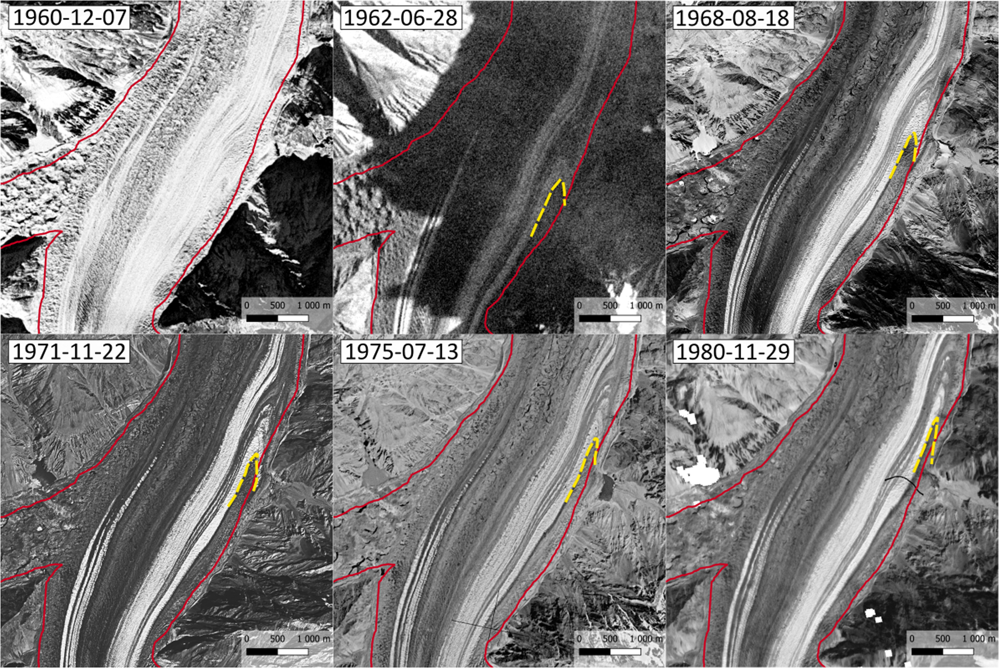
Figure 9. Temporal evolution of a looped-moraine on Fedchenko main trunk, downstream of the confluence with Bivachny Glacier (see Figure 1 for the general location). Images: KH-2, KH-4 and KH-9 series (Table 4). The looped-moraine is highlighted by a yellow dashed line on each image. The identifiable locations of the tip of the looped-moraine are also reported on Figure A7.
The point scale velocity estimates from this method show that the 1962–68 velocity is much larger than all the other velocities estimated at this location, with 137 ± 12 m yr−1 versus velocities from 65 ± 13 to 77 ± 23 m yr−1 for the different periods from 1968 to 1980 (Table 4). The spatial variability of the velocity cannot explain these differences, as the 2017–18 velocity ranges from 49 to 79 m yr−1 at the location of the tip of the looped moraine (Table 4). The looped moraine is located in the vicinity of the historical profile named profile X (Schulz, Reference Schulz1962), where velocity was measured by field techniques from February 1958 until August 1959 (Fig. A7). The mean velocity along profile X for the period 1958–59 is 26.7 cm d−1, corresponding to 97.5 m yr−1 (Schulz, Reference Schulz1962). Given that the looped moraine is located on the side of the glacier, and given the present day observed profile, we can estimate that the velocity at the looped moraine location is ∼75% of the profile average velocity, which would lead to a velocity of ∼73 m yr−1 in 1958–59 (Fig. A7). This value is very close to the velocity estimates of the periods after 1968 (Table 4), but this very good agreement is to be taken with some caution, as we do not know exactly how the profile average velocities were measured in 1958–59 (Schulz, Reference Schulz1962). Unfortunately, the quality of the KH-2 and KH-4 images and the poor co-registration of the whole series of historical images do not allow us to retrieve velocities along the cross section of the tongue. We could thus only track the velocity and velocity changes on the right bank of Fedchenko main tongue.
The analysis of velocities is still uncertain, but it indicates that the velocity close to the confluence with Bivachny was roughly twice as large between 1962 and 1968, than during all the other periods. We calculated a 6 year average that hides large temporal variability in velocity, and it is likely that the peak velocity was much larger. It is also noteworthy that this location of Fedchenko Glacier undergoes significant seasonal variability in velocity, with spring velocities 50% larger than annual averages, which might complicate the analysis (Nanni and others, Reference Nanni, Scherler, Ayoub, Millan, Herman and Avouac2023).
In summary, we gathered the following evidence regarding anomalous flow of Fedchenko Glacier: (1) presence of a looped moraine on the right bank of Fedchenko main tongue; (2) large thinning happening probably from 1960 to 1968; and (3) velocities twice as large as all the other measured velocities during the period 1962–68 on the right bank of Fedchenko main tongue. With respect to (1), the presence of a looped moraine could be explained by the ice discharge from a surging tributary glacier into Fedchenko (Jennings and Hambrey, Reference Jennings and Hambrey2021) or by internal folding (Post, Reference Post1972). Given the location of the looped moraine, the natural candidate would be Kosinenko Glacier, which is a surge-type glacier (Kotlyakov and others, Reference Kotlyakov, Osipova and Tsvetkov1997). On all the historical images, the front of Kosinenko Glacier is located ∼3.8 km away from Fedchenko Glacier. We cannot rule out that Kosinenko Glacier surged before 1960 and retreated quickly, but this seems rather unlikely. Regarding (2) and (3), both observations would point toward a large speed-up of Fedchenko main tongue that happened sometimes between August 1959 and August 1968, but our data are too coarse to properly characterize the spatial extent of the changes or to observe a potential surge front.
The mechanisms that led to this speed-up are completely unclear, but they might be related to pulses of meltwater originating from neighboring surge-type glaciers or might be the result of a surge of Fedchenko Glacier. This acceleration did not lead to a front advance, nor to major flow disturbance, explaining why it was not noticed before, except in Kotlyakov and others Reference Kotlyakov, Osipova and Tsvetkov(1997). The specific surge inventories for the region investigated later periods and thus could not detect this event (Goerlich and others, Reference Goerlich, Bolch and Paul2020, Guillet and others, Reference Guillet, King, Lv, Ghuffar, Benn, Quincey and Bolch2022, Guo and others, Reference Guo, Li, Dehecq, Li, Li and Zhu2023). Given the extremely high density of surging glaciers in the surroundings, it is not very surprising to observe such kind of glacier flow instability.
5.3. The mystery of Jasgulem pass elevation changes
Lambrecht and others Reference Lambrecht, Mayer, Aizen, Floricioiu and Surazakov(2014) already noticed a substantial thinning of more than 30 m for elevations above ∼4700 m a.s.l. for the periods 1928–2000 and 1928–2009. Interestingly, they found that this thinning was increasing with increasing elevation. The data presented in this study show that the 2010–21 pattern is opposite, with decreasing thinning rates with elevation (Fig. 5). Two previous hypotheses were proposed to explain the thinning: reduced accumulation, due to drier conditions that would lead to an imbalance between discharge and surface mass balance, and/or a densification of the firn due to increased temperature (Lambrecht and others, Reference Lambrecht, Mayer, Aizen, Floricioiu and Surazakov2014). The second hypothesis is supported by observations of ice layers in the firn (Lambrecht and others, Reference Lambrecht, Mayer, Bohleber and Aizen2020) but can only partly explain the elevation changes, as the firn densification has a small impact on elevation changes (Ochwat and others, Reference Ochwat, Marshall, Moorman, Criscitiello and Copland2021).
The thinning is most pronounced downstream of Jasgulem pass (Fig. 10), an ice divide between Fedchenko Glacier (NE direction; Fig. 1) and Jasgulem Glacier (SW direction). We report two intriguing features at Jasgulem pass. First, we observe a migration of the topographic divide, ∼100 m toward Jasgulem Glacier between 1928 and 2019 (Fig. 10). The terrain is very flat, leading to high uncertainty on the location of the topographic divide, especially in the 1928 map. The divide migration does not explain the thinning, but instead we observe that the shape of the elevation profile at the divide location has changed (Fig. 10). In particular, we note that the past divide was more prominent, with slightly steeper slopes within 1 km in the downstream direction (Fig. 10).
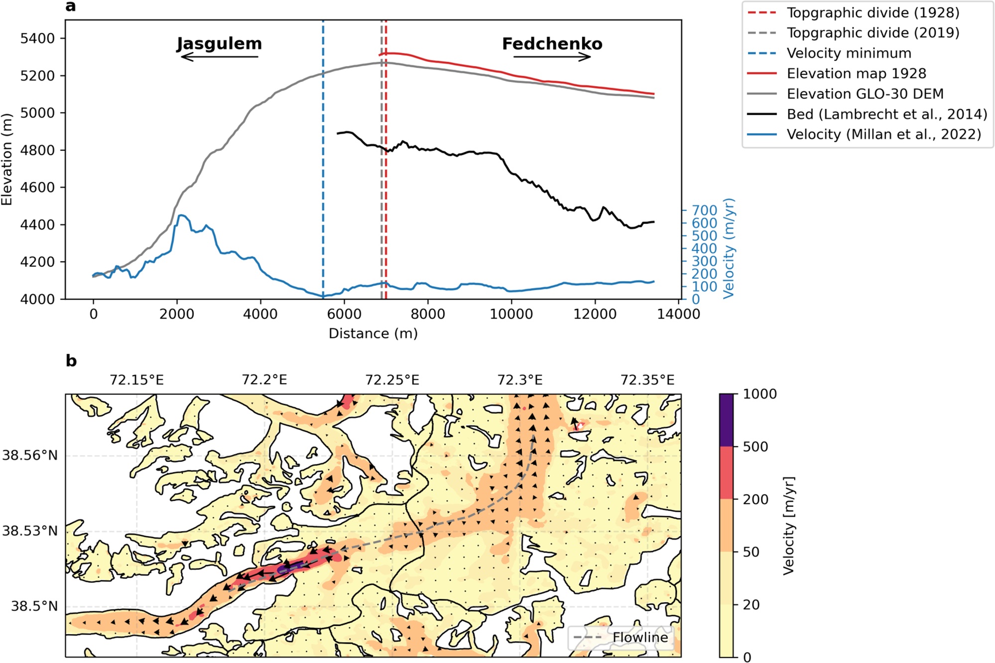
Figure 10. Elevation and velocity along a 14 km flowline crossing Jasgulem pass (a). The dashed vertical blue line shows the minimum velocity (ice divide) and the dashed red and gray lines show the maximum elevation (topographic divide) in 1928 and in 2019, respectively. The Copernicus 30 m DEM (GLO-30DEM; European Space Agency, 2022) elevation is adjusted on the Pléiades 2019 elevation for consistency. The map (b) shows the surface velocity from Millan and others Reference Millan, Mouginot, Rabatel and Morlighem(2022) at the location of Jasgulem pass (solid black line separating the two main glaciers). The gray dashed line shows the flowline profile of panel (a).
Second, we also note that the ice flow divide location does not match with the topographic divide. We identified the ice flow divide location by the minimum in the ice velocity (Millan and others, Reference Millan, Mouginot, Rabatel and Morlighem2022), which is located 1.4 km away from the topographic divide in direction of Jasgulem Glacier (Fig. 10). The location of the ice flow divide is also visible in other data sources, such as ITS_LIVE (Gardner and others, Reference Gardner, Fahnestock and Scambos2024), and seems to be imposed by the bed geometry. Ground penetrating radar measurements show that the glacier bed maximum elevation is not located at the topographic divide (Lambrecht and others, Reference Lambrecht, Mayer, Aizen, Floricioiu and Surazakov2014, Reference Lambrecht, Mayer, Bohleber and Aizen2020, Fig. 10). Jasgulem Glacier is a surge-type glacier, with flow instabilities that are usually confined to the lower elevations (Goerlich and others, Reference Goerlich, Bolch and Paul2020, Guo and others, Reference Guo, Li, Dehecq, Li, Li and Zhu2023). It is possible that the ice dynamics of Jasgulem Glacier may impact the flow of Fedchenko glacier, due to their share of a divide.
5.4. Uncertainties and limitations
Our analysis relies heavily on the analysis of topographic data that originates from multiple sources (historical ground photogrammetric surveys, spy satellite imagery, modern satellite imagery, satellite laser altimetry and GNSS), each referring to different geodetic reference systems, which is particularly true for the historical maps. Despite a careful processing of these data, it remains challenging to assess the uncertainty in a quantitative way, due to the lack of stable terrain. We assessed the impact of the spatial sampling in Section 3 and found a moderate impact for the GNSS data, with a standard deviation of 0.34 m, and a larger impact for ICESat data, with a standard deviation of 0.54 m. We also assess the impact of the seasonal correction applied to the GNSS data. If we do not apply the correction, we find rates of elevation changes 0.06 m yr−1 less negative for the period 2003–09 and 0.11 m yr−1 more negative for the 2016–21 periods, respectively. These results correspond to a 25% error, which would change the interpretation of the results if not applied. The correction is based on only one period of analysis in summer 2019, which is a limitation. Another possibility to validate the data could be the use of ICESat-2 simultaneous overpasses. Unfortunately, there were no suitable ICESat-2 tracks that could be compared to the Pléiades DEM.
Providing highly accurate and spatially complete maps of elevation changes over large glaciers, such as Fedchenko Glacier, is a challenge, even for the most recent sensors. DEMs from SAR sensors, such as TanDEM-X, allow covering large areas at once and are thus well suited. However, they are impacted by the poorly known penetration depth of the X-band signal (Li and others, Reference Li2021). For the specific case of Fedchenko Glacier, the X-band penetration is limited for September acquisitions for elevations below 5400 m a.s.l. (Lambrecht and others, Reference Lambrecht, Mayer, Wendt, Floricioiu and Völksen2018). Time series of ASTER DEMs are also used to calculate geodetic mass balances, but the image correlation shows limited success in the high elevation areas, due to the lack of texture and/or the saturation of the images. This leads to artifacts or voids in the reconstructed DEMs and thus to highly variable rates of elevation changes for three different studies (Fig. 11; Brun and others, Reference Brun, Berthier, Wagnon, Kääb and Treichler2017, Shean and others, Reference Shean, Bhushan, Montesano, Rounce, Arendt and Osmanoglu2020, Hugonnet and others, Reference Hugonnet2021). Commercial optical sensors such as Pléiades or WorldView are less prone to saturation (Berthier and others, Reference Berthier2023), although it can still happen, as visible in the 1–2 August 2019 Pléiades DEM (Table 1). Thanks to their very high resolution (50 cm–1 m of ground sampling distance) and radiometric depth, these sensors capture images with more texture than the lower resolution sensors (Fig. A8). It is thus possible to derive void free DEMs on areas with limited or small surface features. The main limitation of these acquisitions is that they are commercial satellites, with limited user access to the tasking and to the existing archive. Another challenge is the limit of the swath width at 20 km in the case of Pléiades, leading to acquisitions distributed over multiple days to cover a larger glacier such as Fedchenko (Table 1).
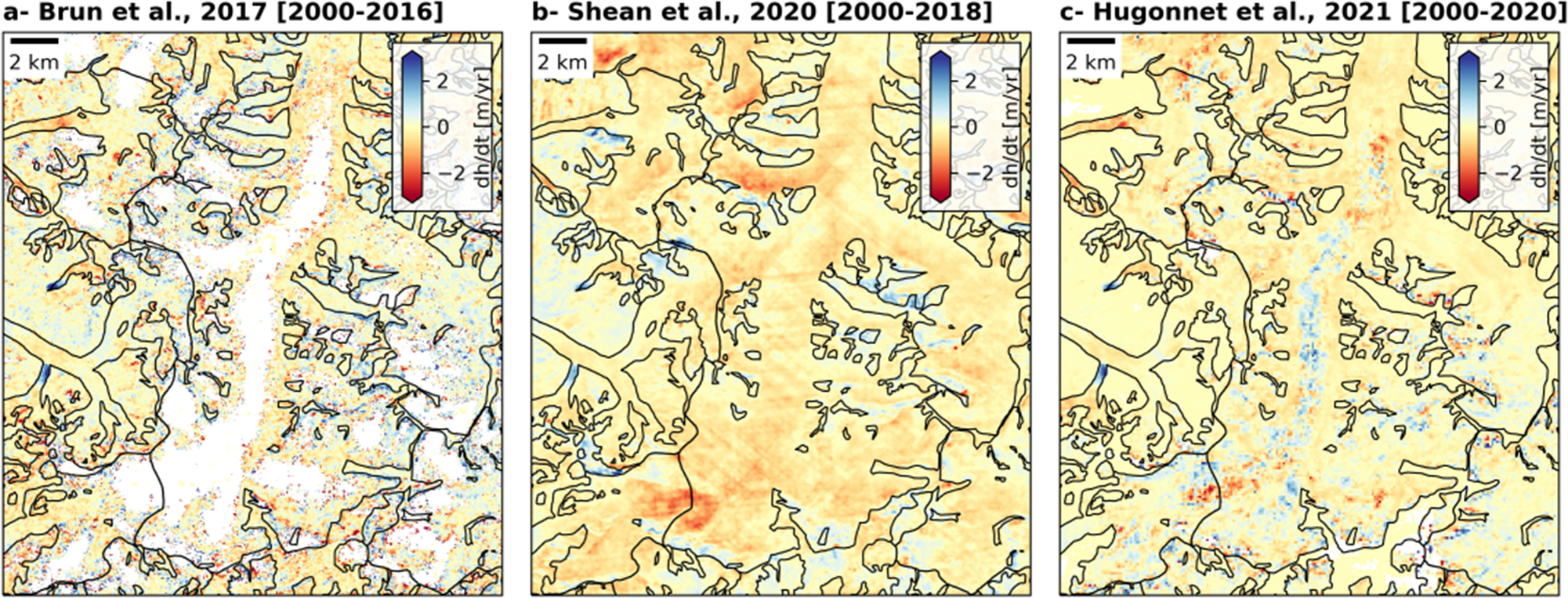
Figure 11. Rates of elevation changes for the higher part of Fedchenko glacier from ASTER-based studies (Brun and others, Reference Brun, Berthier, Wagnon, Kääb and Treichler2017, Shean and others, Reference Shean, Bhushan, Montesano, Rounce, Arendt and Osmanoglu2020, Hugonnet and others, Reference Hugonnet2021).
In this study, we rely on ERA5 data to investigate the temporal changes in meteorological conditions. Barandun and Pohl Reference Barandun and Pohl(2023) showed that relying on different meteorological reanalysis can have an impact on the relative importance of the predictors of glacier mass-balance variability. As ERA5 monthly estimates of temperature, and to a lesser extent precipitation, are in good agreement with the Fedchenko station measurements, we did not investigate other data sources, but it is clear that our analysis could benefit from climate simulations that cover the entire 20th century.
6. Conclusion
In this study, we document more than nine decades of elevation changes of Fedchenko Glacier from 1928 to 2021, in the heart of the data scarce Central Pamir. We use various data sources, including topographic maps, DEMs from optical satellites and GNSS surveys, allowing us to study four distinct sub-periods (1928–58, 1958–80, 1980–2010, 2010–21). These topographic data are combined with meteorological data from Gorbunov Station (1936–94) and ERA5 (1950–2021). Overall, we observe an up-glacier propagation of the thinning rates that are the largest for the most recent period of observation (2010–21). In particular, thinning rates of the accumulation basin reach −0.41 m yr−1 for the period 2016–21. For some periods, it is possible to link the glacier rate of elevation change to climate anomalies. The period 1980–2010 shows limited thinning and even thickening in the accumulation area. This periods corresponds to a wet anomaly that might have limited mass loss. Still, the temporal variability in the rates of elevation changes cannot be fully linked to the climate variability. For instance, for the period 1958–80, we observe large thinning on the tongue of Fedchenko Glacier that seems to be linked to anomalously high velocities akin to a surge event.
Our study highlights both the interest and the limitations of compiling historical and modern topographic elevation data and images. On the one hand, the non-complete maps of elevation changes are unsuitable to calculate the geodetic mass balance of a glacier, but the relative comparison between sub-periods is still highly valuable. We also show that the combination of field measurements, such as GNSS surveys and ground penetrating radar, with remote sensing products (DEMs and surface velocity) is key to study glaciers as large as Fedchenko Glacier, which might be more dynamical than previously thought.
Data availability statement
Elevation change maps are available in form of a Zenodo deposit (Brun, Reference Brun2024).
Acknowledgements
We thank Sajid Ghuffar for sharing the 1968 Corona KH-4 orthoimage and DEM. EB acknowledges support from the French Space Agency (CNES). We thank the Scientific Editor Hester Jiskoot, Tobias Bolch and an anonymous reviewer for their comments which greatly improved the manuscript. Pléiades images were acquired thanks to DINAMIS (Dispositif Institutionnel National d’Approvisionnement Mutualisé en Imagerie Satellitaire) and the Pléiades Glacier Observatory.
Competing interests
Author F.B. is one of the Scientific Editors of the Journal of Glaciology.
Appendix 1.
Table A1. Summary of co-registration of individual DEMs
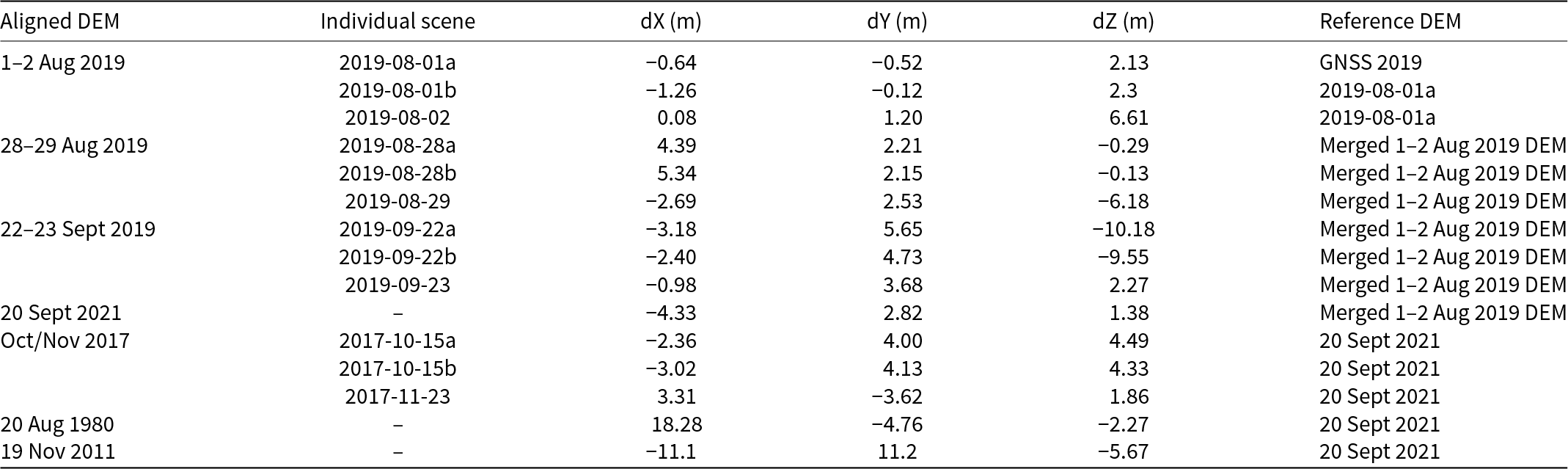
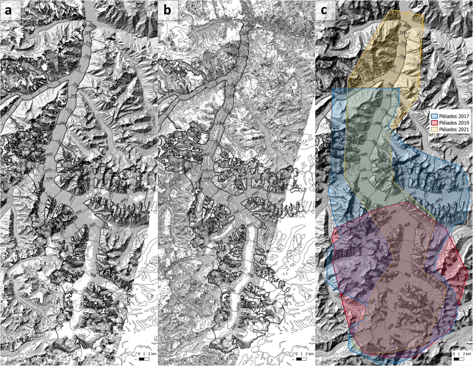
Figure A1. Hillshades from the KH-9 (a) and SPOT 5 (b) DEMs. Panel (c) shows the footprint of the different Pléiades DEMs, with a hillshade from GLO-30 DEM as a background. Note that the Pléiades DEMs are near-complete, especially on the glacierized areas.
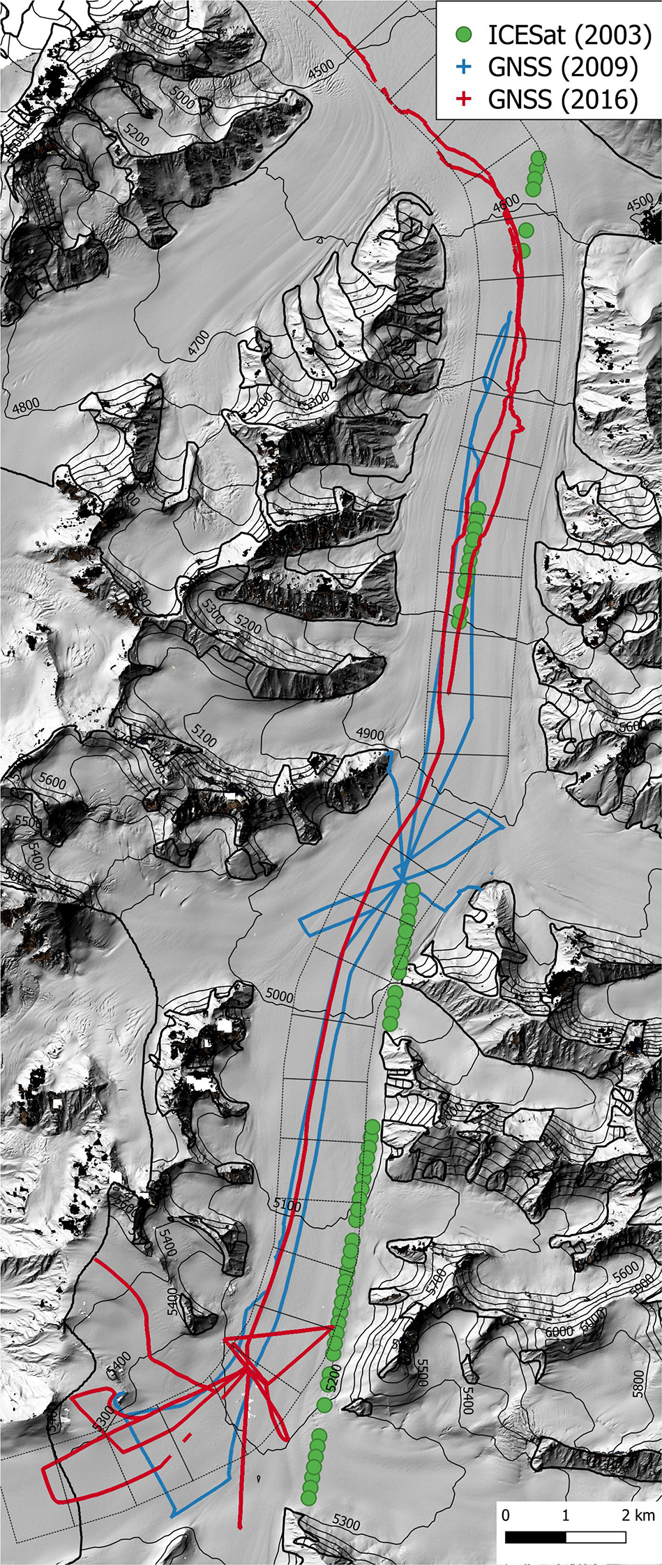
Figure A2. Summary of the ICESat and GNSS acquisitions.
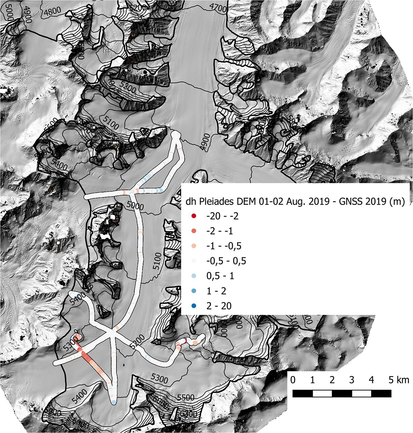
Figure A3. Elevation difference between GNSS measurements from 4 to 17 August 2019 and the average between the Pléiades DEMs of 1–2 and 28–29 August 2019 after co-registration. Note some spurious measurements in one GNSS track that was discarded from the analysis.
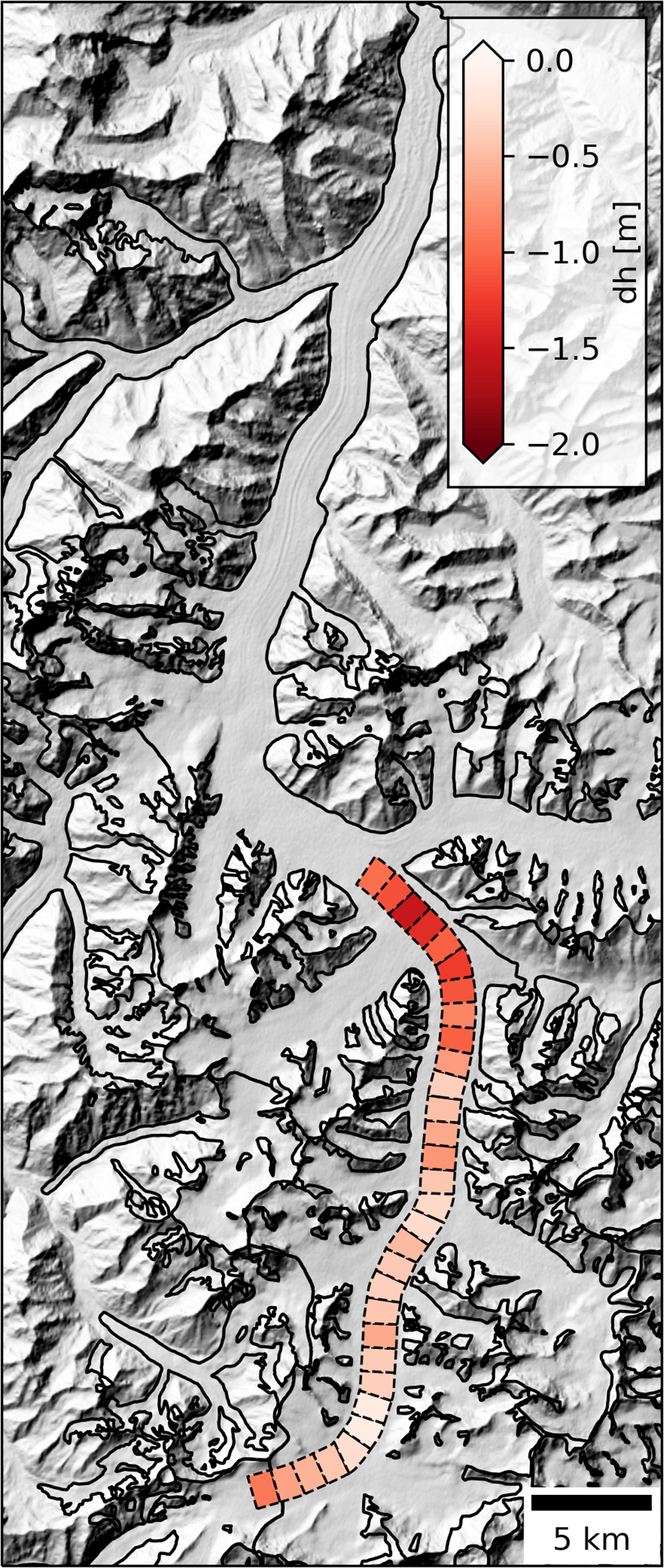
Figure A4. Elevation difference between the Pléiades DEM of 22–23 September 2019 and the Pléiades DEM of 1–2 August 2019 that is used for the seasonal correction of GNSS data.
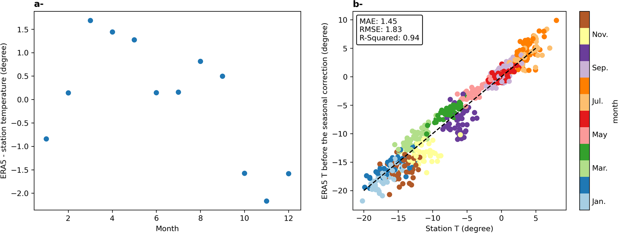
Figure A5. Mean monthly temperature bias in ERA5 data (a) and monthly ERA5 versus the station temperature before seasonal bias correction (b).
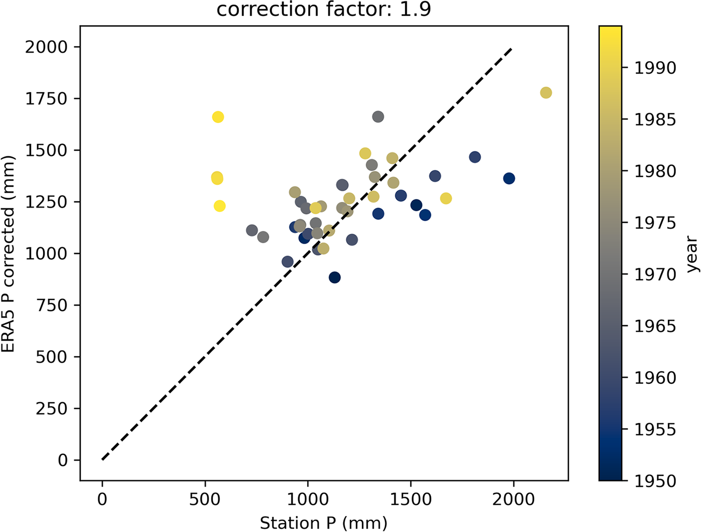
Figure A6. Comparison of the annual ERA5 adjusted precipitation the annual station record for the overlapping years (1950–94). Note the spurious values for the years 1990–94 in the station record. These values were excluded from the analysis.
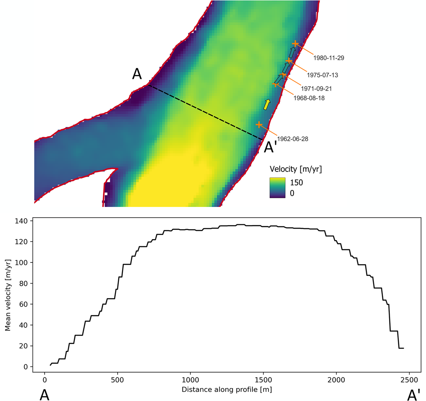
Figure A7. Map of the location of the tip of the looped moraine identified in the spy satellite imagery (Table 4 and Figure 9). The background is the velocity map from Millan and others Reference Millan, Mouginot, Rabatel and Morlighem(2022), and the arrows show the velocity inferred from the looped-moraine tracking. The graph shows the velocity profile along the AAʹ line (corresponding to the approximate location of the X profile) from Millan and others Reference Millan, Mouginot, Rabatel and Morlighem(2022).
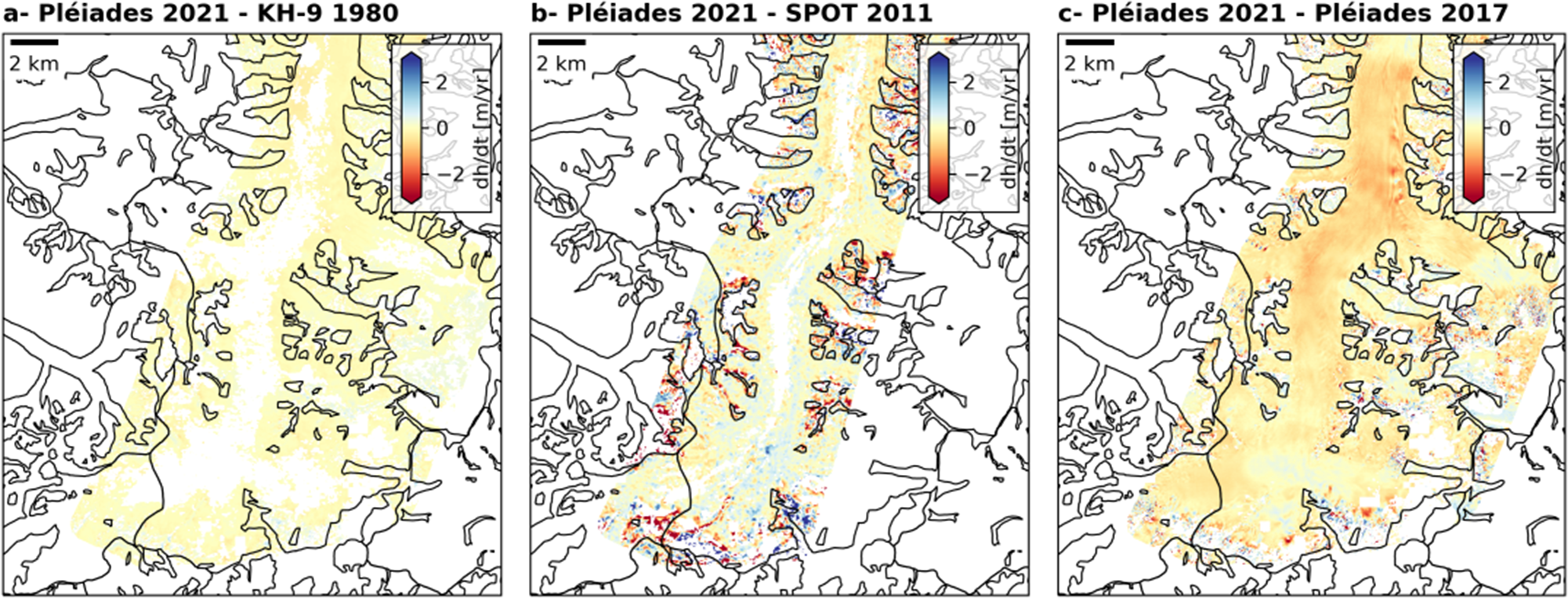
Figure A8. Rates of elevation changes for the higher part of Fedchenko Glacier from differences of DEMs presented in this study. Colorscale and spatial extent are similar to Figure 11.


 Open access