Spatiotemporal variability of air temperature biases in regional climate models over the Greenland ice sheet

Abstract

Regional climate models (RCMs) are fundamental tools in understanding and quantifying the contribution of the Greenland ice sheet to sea-level rise. We perform an extensive evaluation of the daily air temperature simulated by two RCMs, MARv3.12 and RACMO$2.3\text{p}2$, and a global atmospheric reanalysis, ERA5, at 35 locations across the ice sheet over the period 1995–2020. We compare model results to weather station data from two climate networks, focusing on the spatial and temporal variability in mean biases (MBs). All three models perform well at low elevations (<1500 m a.s.l.) with an MB of 0.16^∘C (MAR), $0.36^{\circ}\mathrm{C}$ (RACMO) and $0.41^{\circ}\mathrm{C}$ (ERA5), while warm biases (>1.70$^{\circ}\mathrm{C}$) are found at high elevations (>1500 m a.s.l.). Temperature biases exhibit a strong seasonality, being more pronounced during winter and much smaller during summer ranging from $0.11^{\circ}\mathrm{C}$ to $0.59^{\circ}\mathrm{C}$. No interannual variability is found in the biases of all three datasets. Daily variability within each month is captured well by both climate models and the reanalysis at most locations. Finally, all three models perform overall better in the ablation zone during summer, i.e. where and when considerable melt production occurs.

1. Introduction

The Greenland ice sheet is a major contributor to sea-level rise with $0.65 \pm 0.09$ mm yr⁻¹ (±90% confidence interval) over the period 1993–2018 (Frederikse and others, 2020) or about 15% of the global mean sea-level rise (Cazenave and others, 2018). Projections indicate further contributions of 0.11–0.25 m by 2300 under low emission scenarios (RCP2.6/SSP1-2.6) and 0.31–1.74 m under high emission scenarios (RCP8.5/SSP5-8.5) (Fox-Kemper and others, 2021).

Regional climate models (RCMs), such as the Modèle Atmosphérique Régionale (MAR, Fettweis and others (2017)) and the Regional Atmospheric Climate Model (RACMO, Noël and others (2018)), are important tools to understand and quantify the ice sheet’s contribution to sea-level rise (Fettweis and others, 2020). Forced by global atmospheric reanalysis data or general circulation models, RCMs are used to model the surface energy balance and melt over the entire Greenland ice sheet, allowing for present-day simulations, past reconstructions and future projections of its contribution to sea-level rise.

Evaluation of RCMs across the entire ice sheet is a fundamental step to ensure that the spatiotemporal variability of the simulated processes is modeled accurately. RCMs are typically compared to in situ observations such as near-surface meteorological data from automatic weather stations (AWSs), surface mass-balance measurements or remote sensing data (e.g. used to derive the extent of bare ice area and/or estimates of mass changes through gravimeters and altimeters). However, previous efforts in evaluating RCMs are often limited, both spatially and temporally, mostly due to scarcity of available in situ observations (Noël and others, 2016; 2019; Fettweis and others, 2017; Reeves Eyre and Zeng, 2017; Delhasse and others, 2020; Zhang and others, 2022). Models are often evaluated with observational data aggregated over the whole ice sheet and/or the entire study period for which data are available. Of these efforts, only Reeves Eyre and Zeng (2017) tried to systematically investigate temporal trends in near-surface temperature biases and spatially distinguished their analysis between low (<1500 m a.s.l.) and high (>1500 m a.s.l.) elevations sites. Unfortunately, this study mostly focused on global reanalyses rather than RCMs, including only MARv3.5.2 in its comparison. While these approaches are straightforward, much more information on the skill of RCMs can be obtained from evaluating results at finer temporal and spatial scales, e.g. at single sites or during different time periods. Furthermore, RCMs and global reanalysis datasets are in continuous evolution, with new releases every year.

In this study, we focus on two state of the art RCMs specifically used to produce estimates and projections of sea-level rise from the Greenland ice sheet, MARv3.12 (Mankoff and others, 2021) and RACMO $2.3\text{p}2$ (Noël and others, 2019). We assess the spatial and temporal variability of these RCMs based on near-surface daily temperature mean biases (MBs) over the entire Greenland ice sheet between 1996 and 2020 by comparing them to observations from the PROMICE (van As and others, 2011) and GC-Net climate networks (Steffen and Box, 2001). For completeness, we also include in our analysis the global reanalysis product ERA5 (Hersbach and others, 2020), which is used to force both MAR and RACMO. We examine the spatial variability in mean model biases evaluating seasonal and interannual changes as a function of latitude, longitude and elevation, where we use 1500 m a.s.l as a threshold to separate observations in the ablation zone from the accumulation zone.

2. Data and methods

2.1. MAR

The MAR is an RCM based on the atmospheric model by Gallée and Schayes (1994) and fully coupled with the soil–ice–snow energy balance vegetation model SISVAT by Gallée and others (2001). Detailed descriptions of the MAR model and its surface and subsurface scheme SISVAT are given in Fettweis and others (2017) and Reijmer and others (2012). In this study, we use MARv3.12 at a spatial resolution of 10 km and forced with ERA5 reanalysis data (Hersbach and others, 2020) every 6 hours. The dataset, including changes from previous versions of the model, is presented in Mankoff and others (2021) while a detailed general description of MAR is given in Fettweis and others (2017). Finally, it is important to note that each new version of MAR is calibrated using PROMICE-based surface mass-balance observations along with satellite-derived melt extent data. However, near-surface temperature in the accumulation zone does not impact significantly these fields and is, therefore, not considered a key field used to calibrate the model (Haacker and others, 2024). It is afterward only used to validate the model (Fettweis and others, 2017; 2020).

2.2. RACMO

The RACMO is an RCM based on the High Resolution Limited Area Model (Undén and others, 2002) and the physics of the European Centre for Medium-Range Weather Forecasts–Integrated Forecast System (ECMWF, 2009), including a snow module that accounts for subsurface processes (Ettema and others, 2010). In this study, we use RACMO $2.3\text{p}2$ (where p stands for polar) at a spatial resolution of 5.5 km and forced with ERA5 reanalysis data (Hersbach and others, 2020) every 6 hours. The dataset is presented in Noël and others (2019) while a detailed description of the model is given in Noël and others (2018). It is important to note that RACMO $2.3\text{p}2$ is not calibrated for improved representation of near-surface temperature.

2.3. ERA5

The ERA5 is the fifth and most recent generation of reanalysis products made available by the European Centre for Medium-Range Weather Forecasts (ECMWF). A full description of ERA5 model and improvements compared to its predecessors are listed in Hersbach and others (2020). Because of its higher vertical and spatial resolution (∼15 km over Greenland), it has been questioned whether this product could replace the use of RCMs like MAR or RACMO. However, Delhasse and others (2020) found out that RCMs forced with ERA5, like the two used in this study, are still better performing at downscaling near-surface climate over the Greenland ice sheet.

2.4. Weather station observations

We use daily mean weather station observations from two Greenland ice sheet wide climate networks (Fig. 1 and Table 1): the Greenland Climate Network (GC-Net) and the Programme for Monitoring of the Greenland Ice Sheet (PROMICE). GC-Net and PROMICE data are neither assimilated in MAR nor in RACMO guaranteeing the independence between modeled and observed air temperatures. However, it is important to note that GC-Net data are assimilated in the production of the ERA5 global reanalysis.

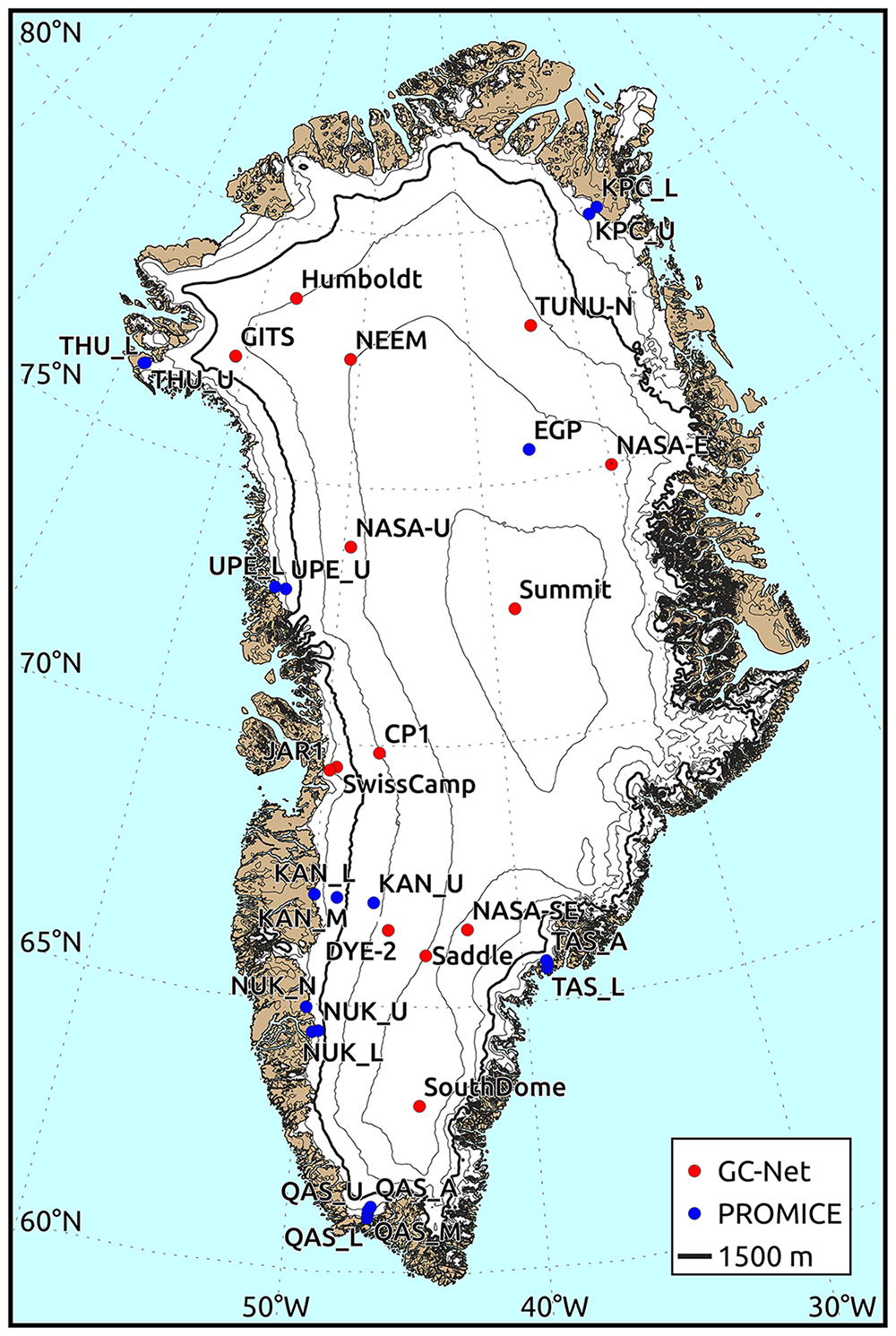
Figure 1. Map of the Greenland ice sheet with the GC-Net and PROMICE weather stations used in this study. Elevation contours based on the ArcticDEM 1 km v3.0 product by the Polar Geospatial Center (Porter and others, 2018) are shown at 500 m intervals (thin black lines) with the 1500 m contour highlighted by thick lines. The ice sheet extent (white) is based on Howat and others (2014).

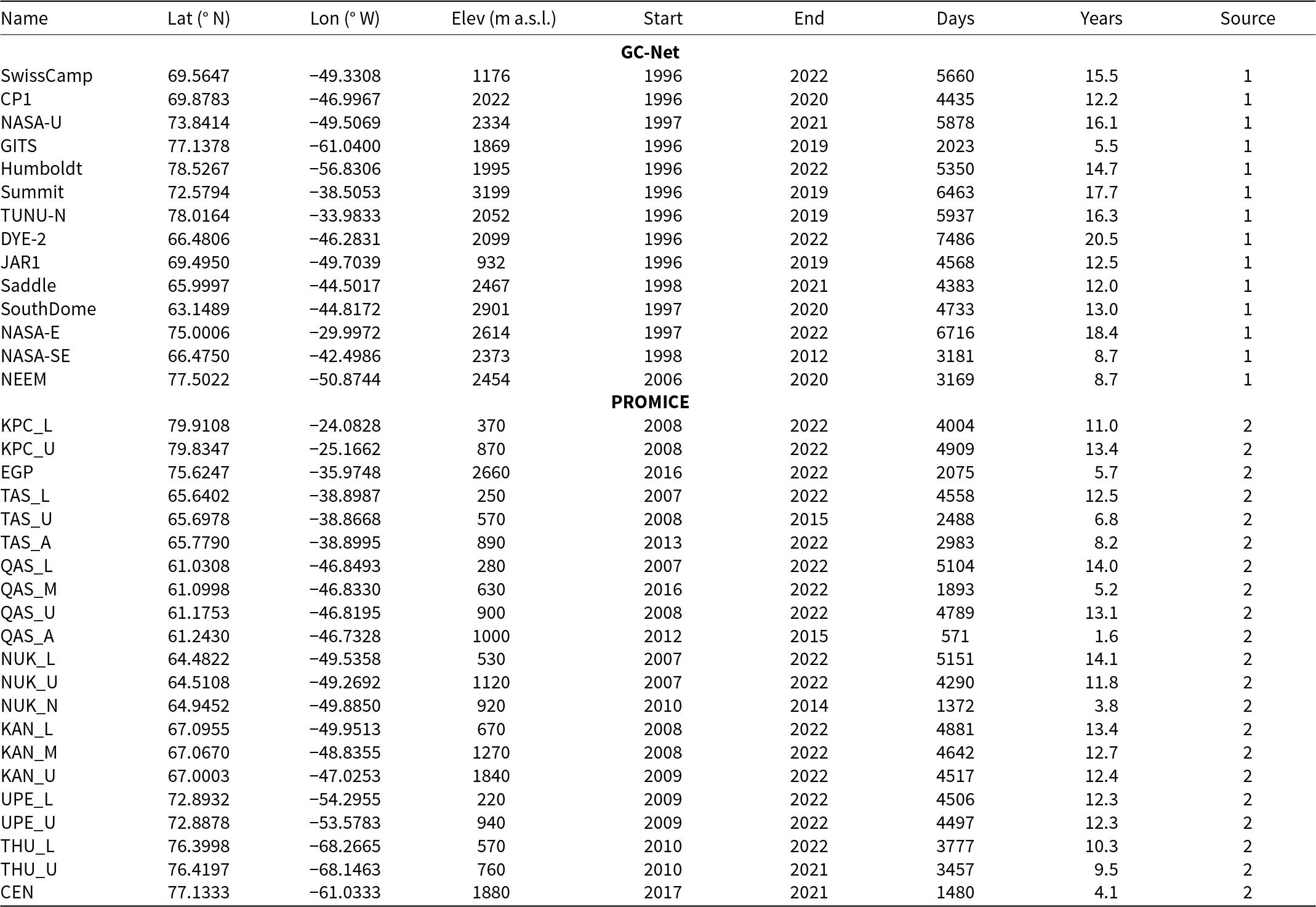
Table 1. Weather stations from the GC-Net and PROMICE networks used in this study. Start and end denote the years with the first and the last temperature observation used in this study, respectively. Days refers to the number of days used in the analysis and years to the equivalent number of years. Elevation (Elev) for each site is taken from the networks metadata (van As and others, 2011; Steffen and others, 2023). Source refers to: 1 Vandecrux and others (2023) and 2 van As and others (2011)

The first GC-Net stations were deployed in 1995, making it the longest-running network over the ice sheet with >25 years of data (Steffen and Box, 2001). Most of these stations are located in the accumulation zone (e.g. at elevations >1500 m a.s.l.). Air temperature is measured at two levels above surface, roughly between 0.5 and 4 m, with a Vaisala CS-500 ( $\pm 0.1^{\circ}\mathrm{C}$) and a Type-E Thermocouple ( $\pm 0.1^{\circ}\mathrm{C}$) at each level, both of which are unventilated. We use the GC-Net augmented level-1 (L1) dataset from Vandecrux and others (2023) archived at Steffen and others 2023 which provides air temperature at 2 m linearly interpolated from the observations at two levels. Furthermore, this dataset has been extensively quality controlled.

The PROMICE weather station network started in 2007 and it currently includes 25 sites mostly located in the ablation zone (e.g. at elevations <1500 m a.s.l.) of outlet glaciers (van As and others, 2011). Air temperature is measured at one level above the surface, at roughly 2 m, with a Rotronic MP100H and a Rotronic HygroClip S3 both mounted in an artificially ventilated Rotronic assembly. We use the MP100H measurements, which are provided quality-checked.

We exclude from our analysis all stations that are located on glaciers outside the ice sheet (three PROMICE stations) and the stations for which the difference between the site elevation and the one interpolated from either model exceeds 100 m (two PROMICE stations in East Greenland). These stations are not shown in Fig. 1 nor listed in Table 1. The average difference (±RMSE) between the model grid elevation and the actual elevation derived from on site GPS measurements is $-14 \pm 43$ m for MAR and $-16 \pm 42$ m for RACMO. A total of 35 stations are used in this study (Table 1), 14 from the GC-Net network and 21 from the PROMICE network.

2.5. Data analysis

For simplicity, in this study, when we refer to models, we include both RCMs, MAR and RACMO, and the global reanalysis ERA5. At each station, daily mean 2 m air temperatures from the models were compared to the weather station data. Model data were interpolated to each weather station site following a linear distance-weighted average of the four nearest grid point values. We computed the MB (model − observed temperatures), root-mean-square error (RMSE), correlation coefficient (r) and the p-value (p). This approach is similar to that used in previous studies (Fettweis and others, 2017; Zhang and others, 2022) and often considered a better approach to using the nearest model gridcell as often done in other validation studies (Noël and others, 2019). However, we investigated the spatial and temporal patterns in air temperature bias with particular attention to altitudinal, latitudinal and longitudinal trends as well as annual and interannual variability. We refer to the four seasons in a year as follows: March, April, May (MAM); June, July, August (JJA); September, October, November (SON); and December, January, February (DJF).

3. Results

Combining the data from all sites and over the entire study period (138 361 daily means; Fig. 2 and Table 2) reveals that all three models show a warm bias compared to observations with a mean of $0.89^{\circ}\mathrm{C}$ for MAR, $1.04^{\circ}\mathrm{C}$ for RACMO and $1.11^{\circ}\mathrm{C}$ for ERA5. The correlation between modeled and measured temperatures is very strong (r > 0.95) and statistically significant (p < 0.01) for all models. However, the RMSE is large for all three models ( $3.0 \pm 0.3^{\circ}\mathrm{C}$). When considering the JJA period in isolation (red dots in Fig. 2), both MB and RMSE for the summer period are considerably lower for all models, by $0.74^{\circ}\mathrm{C}$ and $1.10^{\circ}\mathrm{C}$ on average respectively.

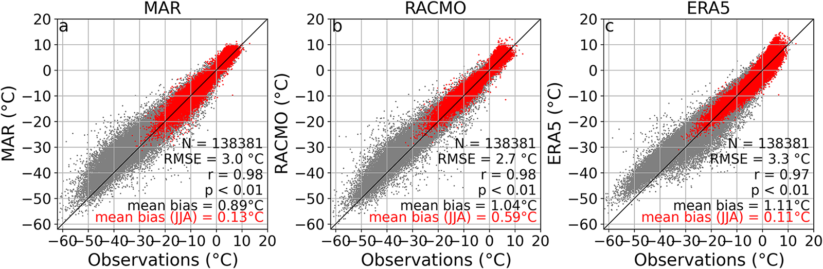
Figure 2. Mean daily 2 m air temperatures from (a) MAR, (b) RACMO and (c) ERA5 versus weather station observations over the entire study period (1996–2020) and for all the sites. Data for the June to August (JJA) period are shown in red and the 1:1 line is given in black. N is the number of samples, RMSE the root-mean-square error, r the correlation coefficient and p the p-value.

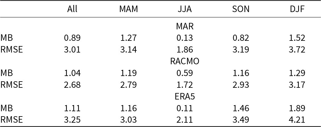
Table 2. Mean bias (MB, ^∘C) and root-mean-square error (RMSE, ^∘C) in 2 m air temperature between models (MAR, RACMO and ERA5) and daily observations at all sites for the whole study period (all) and the four seasons

3.1. Spatial variability

With most stations’ data coverage spanning >10 years (only three stations have <5 years of data, Table 1), we have a sufficiently long temporal range to estimate meaningful MBs at each individual site (Fig. 3 and Table S1). Maps of MB (Fig. 3a–c) show that for all models the annual MB is smaller at sites located at low elevations (<1500 m a.s.l.) near the ice sheet margin, e.g. in the ablation zone. Here, the annual MB ranges from $-1.20^{\circ}\mathrm{C}$ to $1.59^{\circ}\mathrm{C}$ in MAR, from $-1.08^{\circ}\mathrm{C}$ to $1.36^{\circ}\mathrm{C}$ in RACMO and from $-2.63^{\circ}\mathrm{C}$ to $2.15^{\circ}\mathrm{C}$ in ERA5 (Table S1) with most values between $\pm 0.5^{\circ}\mathrm{C}$. However, at high elevations (>1500 m a.s.l.), e.g. in the accumulation zone, large positive annual MBs can be found, with values up to $2.61^{\circ}\mathrm{C}$ in MAR, $2.95^{\circ}\mathrm{C}$ in RACMO and $2.76^{\circ}\mathrm{C}$ in ERA5.

Figure 3. Maps of mean bias in 2 m air temperature in (a, d–g) MAR, (b, h–k) RACMO and (c, l–o) ERA5 compared to daily observations at 35 sites (a–c) over the entire study period and (d–o) for four seasons. The 1500 m contour (black line) is from the ArcticDEM (Porter and others, 2018) and the ice sheet extent (gray line) is based on Howat and others (2014).

We further investigate the spatial variability by plotting the MB against elevation, latitude and longitude (Fig. 4, where blue and red circles indicate low and high elevations sites). All models indicate that the MB increases with increasing elevation, with a trend of $0.81^{\circ}\mathrm{C}$ km⁻¹ in MAR, $0.75^{\circ}\mathrm{C}$ km⁻¹ in RACMO and $1.01^{\circ}\mathrm{C}$ km⁻¹ in ERA5, respectively (Fig. 4a–c), with linear regressions showing a moderate but statistically significant correlation (p < 0.01) for all models (r = 0.79 for MAR, r = 0.73 for RACMO, r = 0.60 for ERA5). While for MAR and RACMO, the MB increase with elevation is steady and constant, for ERA5, the transition from a negative to a positive MB is notably steep below 1000 m a.s.l., stabilizing at approximately $2^{\circ}\mathrm{C}$ above 1000 m a.s.l. (Fig. 4c). No significant trend is found with either latitude (Fig. 4d–f) or longitude (Fig. 4g–i). The scatter is considerably larger than for the elevation dependency, and the magnitude of the MB is again controlled by its elevation rather than by its latitude or longitude as shown by the blue (low elevation sites) and red (high elevation sites) circles in Figure 4.

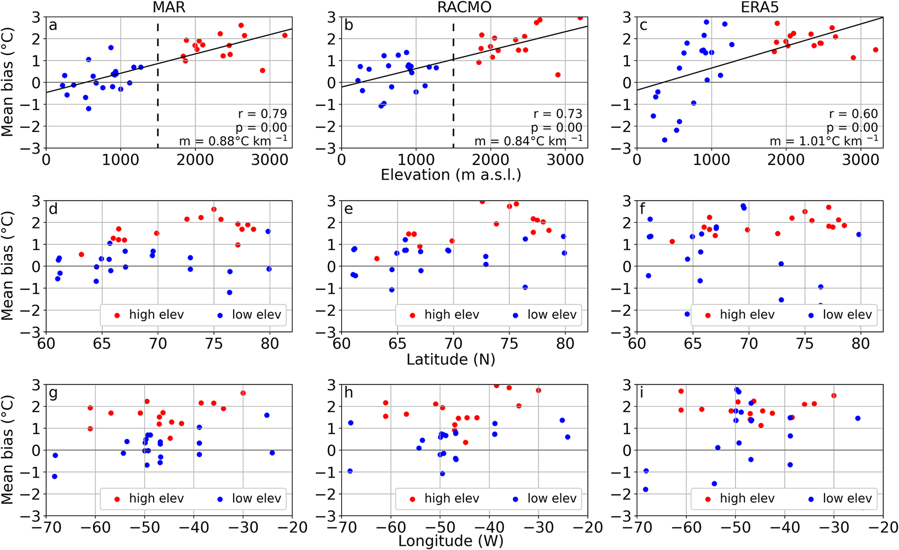
Figure 4. Mean bias in 2 m air temperature between models, (a, d, g) MAR, (b, e, h) RACMO and (c, f, i) ERA5, and daily observations plotted against (a–c) elevation, (d–f) latitude and (g–i) longitude for each site over the entire study period (1996–2020). Low elevation sites (<1500 m a.s.l.) are shown in blue and high elevation sites (>1500 m a.s.l.) in red. In (a–c), linear regressions are shown in solid lines, r is the correlation coefficient, p the p-value and m the slope. The dashed black line in (a, b) highlights the 1500 m elevation.

3.2. Temporal variability

MBs computed for each of the four seasons (Fig. 3d–o) reveal a strong annual seasonality in all models. Both mean seasonal bias and RMSE computed over all the sites are larger during the winter time (DJF) and smaller during the summer (JJA) (Table 2). Because of the strong elevation dependency in MB found above, we further distinguish between sites at high elevation (>1500 m a.s.l.) and low elevation (<1500 m a.s.l.). While seasonal variations are absent at low elevations, the seasonality is amplified at high elevations (Fig. 5), with monthly MB ranging from $-0.30^{\circ}\mathrm{C}$ to $3.28^{\circ}\mathrm{C}$ in MAR, from $0.66^{\circ}\mathrm{C}$ to $2.52^{\circ}\mathrm{C}$ in RACMO and from $-0.44^{\circ}\mathrm{C}$ to $3.96^{\circ}\mathrm{C}$ in ERA5. The amplitude of the annual seasonality is the largest in ERA5, followed by MAR and then RACMO (Figs. 3 and 5).

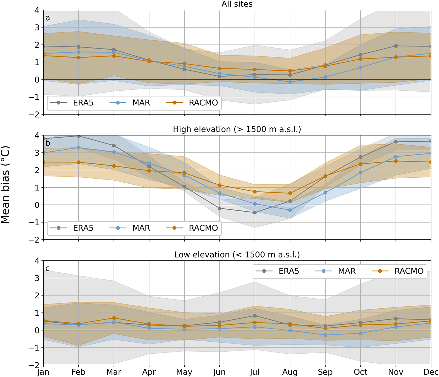
Figure 5. Monthly mean bias in 2 m air temperature and standard deviation (shaded) between models (MAR, RACMO and ERA5) and observations at (a) all sites, (b) high elevation sites and (c) low elevation sites.

Interpreting the spatial difference in seasonality requires care since the two weather station networks used in this study cover different time periods and different areas of the Greenland ice sheet. GC-Net data cover almost all of the study period and these stations are almost entirely located at high elevation (>1500 m a.s.l., Table 1). PROMICE data are available starting from 2007 and these stations are almost entirely located at low elevation (<1500 m a.s.l., Table 1).

Figure 6 shows the annual MB and standard deviation in 2 m air temperature between models and observations. When considering years with $ \gt \sim$10 stations available for the calculations, the annual MB (Fig. 6) does not show a trend as evident as the seasonality shown by the monthly MB. At high elevation, annual MB ranges from $1.23^{\circ}\mathrm{C}$ to $2.30^{\circ}\mathrm{C}$ in MAR, from $1.20^{\circ}\mathrm{C}$ to $2.02^{\circ}\mathrm{C}$ in RACMO and $1.23^{\circ}\mathrm{C}$ to $2.50^{\circ}\mathrm{C}$ in ERA5 (Fig. 6b). At lower elevations, annual MB ranges from $-0.26^{\circ}\mathrm{C}$ to $0.41^{\circ}\mathrm{C}$ in MAR, from $-0.02^{\circ}\mathrm{C}$ to $0.65^{\circ}\mathrm{C}$ in RACMO and from $0.00^{\circ}\mathrm{C}$ to $0.59^{\circ}\mathrm{C}$ in ERA5 (excluding years prior to 2008 when only two GC-Net stations were operational, Fig. 6c). These results confirm once more the strong elevation dependency of the air temperature MB, with greatest biases at the higher elevations.

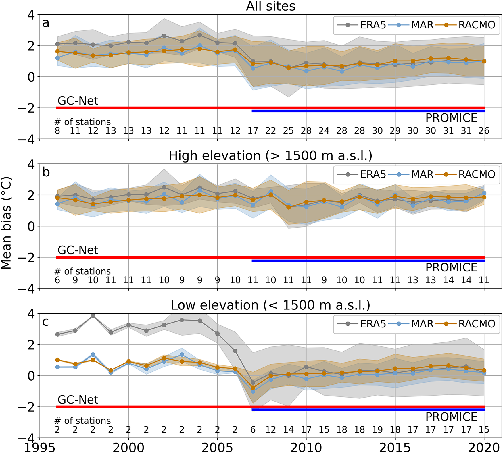
Figure 6. Annual mean bias in 2 m air temperature and standard deviation (shaded) between models (MAR, RACMO and ERA5) and observations at (a) all sites, (b) high elevation sites and (c) low elevation sites. Data coverage is shown for the GC-Net (red) and PROMICE (blue) weather stations network. The number of stations from which each annual mean is computed is also shown (# of stations).

When the data from all sites are included (Fig. 6a), the annual MB shows a clear step-like drop in 2007 and remains relatively constant thereafter. This drop coincides with the first year in which the first PROMICE stations were deployed, complementing the only two GC-Net stations located at elevations <1500 m a.s.l. The decrease in annual MB is due to the overall smaller biases at PROMICE sites which are located at low elevations.

3.3. Daily variability

To assess the skill of the models in simulating daily variability throughout the year, we examine the distribution of daily mean air temperature in each month for MAR, RACMO, ERA5 and the observations for high elevation and low elevation sites (Fig. 7). Two patterns in both observations and models emerge from this analysis: first, air temperature variability is larger during winter and smaller during summer; and second, variability is larger at high elevation (Fig. 7a) than at low elevation (Fig. 7b). All models capture well the daily variability in air temperature at both high and low elevations and in all months of the year. Median values reflect what is shown by the MB analysis above, i.e. the models have a warm bias especially at high elevations and during the winter (Fig. 7a). Both the interquartile range, which contains 50% of the data, and the lower to upper whisker range, which contains 99.3% of the data, compare very well between the models and the observations (Fig. 7).

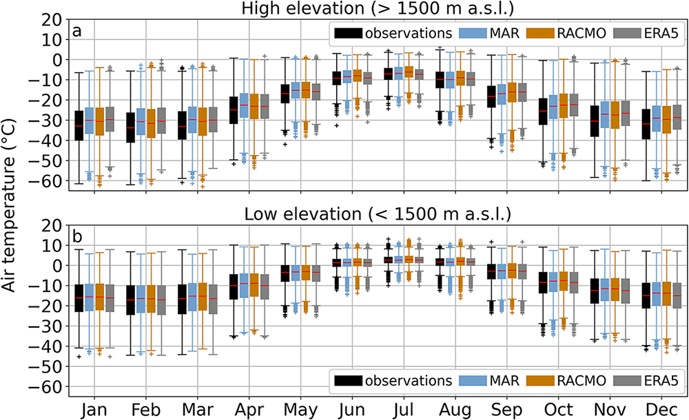
Figure 7. Boxplot of monthly 2 m air temperature from observations and models (MAR, RACMO and ERA5) at (a) high elevation sites and (b) low elevation sites. Median is shown with a red line, 1st and 3rd quartiles with a box, lower and upper whiskers with colored lines and outliers as a cross.

4. Discussion

Air temperature biases show a strong dependency on elevation in all models (MAR, RACMO and ERA5), while no dependency is found with latitude or longitude (Fig. 4a, b). The mean model bias is 0.16, 0.36 and $0.41^{\circ}\mathrm{C}$ at elevations <1500 m a.s.l. and 1.71, 1.79 and $1.89^{\circ}\mathrm{C}$ at elevations >1500 m a.s.l., for MAR, RACMO and ERA5, respectively. This dependency on elevation recurs in all the statistical analyses performed. A strong seasonality in MB is found only at high elevations (Fig. 5), and annual MBs are higher at elevations >1500 m a.s.l. (Fig. 6).

When compared to previous studies, our results reveal in general greater biases for all three models. For MARv3.5, forced with ERA-Interim reanalysis data, Fettweis and others (2017) found a negative MB of $-0.29^{\circ}\mathrm{C}$ (validation at 12 PROMICE stations over the period 2008–10), while Reeves Eyre and Zeng (2017) found a positive MB of $1.38^{\circ}\mathrm{C}$ (validation at PROMICE, GC-Net and other available stations over the period 1958–2015, e.g. coastal stations from the Danish Meteorological Institute). For MARv3.9, forced with ERA5 reanalysis data, Delhasse and others (2020) found an MB of $0.06^{\circ}\mathrm{C}$ (validation at 21 PROMICE stations over the period 2010–16) compared to the bias of $0.98^{\circ}\mathrm{C}$ in this study. For RACMO $2.3\text{p}2$, forced with ERA-Interim reanalysis data, Noël and others (2019) found an MB of $0.14^{\circ}\mathrm{C}$ (validation at 18 PROMICE and 5 IMAU stations over the period 2007–16), while Zhang and others (2022) found an MB of $1.0^{\circ}\mathrm{C}$ using monthly data (validation at 20 PROMICE stations over the period 2007–20) compared to the $1.04^{\circ}\mathrm{C}$ in this study. For ERA5 global reanalysis, Delhasse and others (2020) found an MB of $0.01^{\circ}\mathrm{C}$ (validation at 21 PROMICE stations over the period 2010–16), while Zhang and others (2022) found an MB of $2.0^{\circ}\mathrm{C}$ using monthly data (validation at 20 PROMICE stations over the period 2007–20) compared to the $1.11^{\circ}\mathrm{C}$ in this study. However, the comparison is not straightforward and our results should not be interpreted as the models’ skill has deteriorated from previous studies. Instead the reason for the higher bias in our study can be explained by differences in study design, since previous studies often only analyzed the PROMICE stations, used different model versions forced with different datasets, and validations were performed over different time periods. If we consider only PROMICE stations in our analysis, we find MBs (±RMSE) of $0.23 \pm 2.29^{\circ}\mathrm{C}$ for MAR, $0.44 \pm 2.15^{\circ}\mathrm{C}$ for RACMO and $0.22 \pm 2.94^{\circ}\mathrm{C}$ for ERA5 (Fig. 8), which are still warmer than previous studies but much smaller than the results including GC-Net stations.

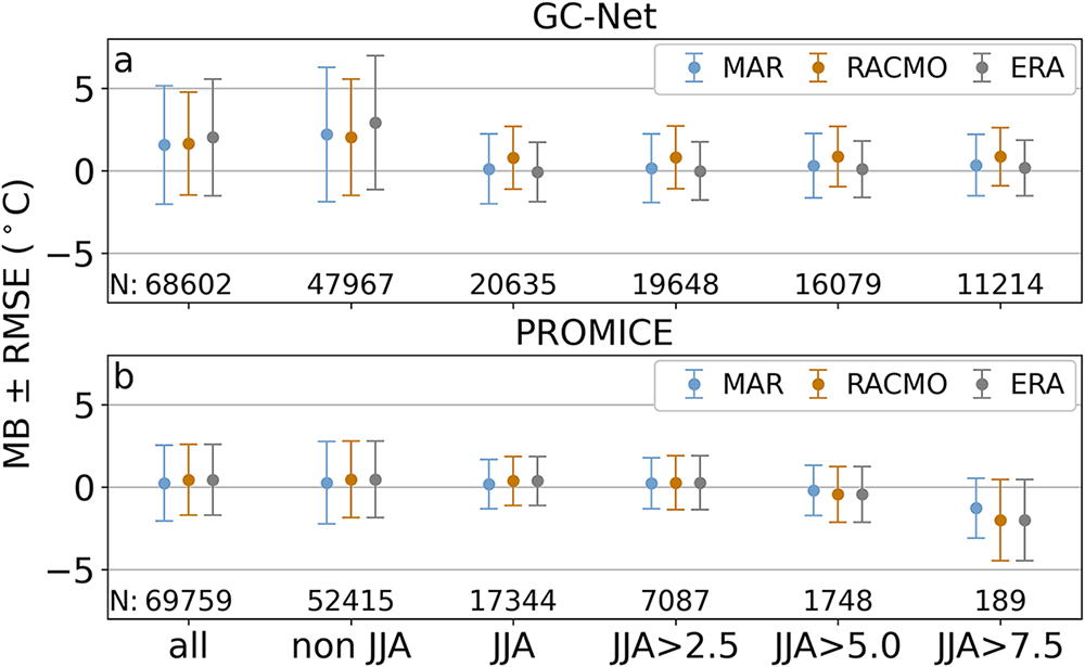
Figure 8. Mean bias (MB) and root-mean-square error (RMSE) in 2 m air temperature between models (MAR, RACMO and ERA5) and the (a) GC-Net and (b) PROMICE climate networks computed over the whole study period (all), over the period between September and May (non JJA), over the summer (JJA) and over the summer but using only days with average wind speed greater than 2.5, 5.0 or 7.5 m s⁻¹ (e.g. JJA > 2.5 m s⁻¹, etc.). Sample number (N) is shown at the bottom of each plot.

A key difference between the two AWS networks is that PROMICE stations are mostly located at low elevations (<1500 m a.s.l.) while GC-Net stations are at high elevations (>1500 m a.s.l.). This explains why, when GC-Net stations are removed from the analysis, the biases decrease as most of the warm biases are found at higher elevations. A possible reason for the greater warm bias at higher elevations is the daily variability in air temperature. Larger variability at high elevations during the winter (Fig. 7) could in fact lead to higher biases. However, all models capture well the daily variability (Fig. 7). Another possible explanation is that models are continuously developed to improve surface mass-balance representation compared to in situ measurements (Fettweis and others, 2017; Noël and others, 2018), which are mostly located at lower elevations, in the ablation zone where most of the melt occurs. However, model tuning typically does not involve air temperature calibration. Furthermore, GC-Net stations data are assimilated in the ERA5 reanalysis; yet the MB at GC-Net stations for ERA5 is larger than for MAR and RACMO (Fig. 8a). Finally, warm biases could be explained by systematically erroneous colder air temperature observations at the GC-Net stations, e.g. by riming or sensor burial by snow during winter. However, the augmented L1 GC-Net dataset was carefully quality controlled in order to avoid erroneous data due to external factors like sensors burial and riming (Vandecrux and others, 2023). Furthermore, while warmer air temperature observations could be physically explained (e.g. by the use of unventilated sensors, discussed in detail in the next section), it is hard to explain consistently colder air temperature measurements observed in this study.

When discussing possible bias sources in the models, the most obvious one is that both MAR and RACMO are forced with ERA5 data, hence the biases in the two RCMs could be directly inherited by the forcing dataset (e.g. Figs 3 and 5). However, both MAR and RACMO include boundary layer parameterizations which are independent of the forcing dataset, making them sensitive to ERA5 biases only in the free atmosphere. It could be the case that near-surface biases are corrected by RCMs if the free atmosphere is well represented in ERA5.

When considering model resolution, all three models differ substantially with a resolution of 5.5 km for RACMO, 10 km for MAR and 15 km for ERA5 (over Greenland). When looking at the whole ice sheet, model resolution doesn’t seem to affect the MB; however, RMSE decreases with finer resolution ( $2.7^{\circ}\mathrm{C}$ for RACMO, $3.0^{\circ}\mathrm{C}$ for MAR and $3.3^{\circ}\mathrm{C}$ for ERA5). Model resolution becomes more important at lower elevations, where the topography is more complex, compared to higher elevations where the ice sheet is generally flatter and more uniform. This is evident in Figure 4c, where ERA5 clearly underestimates the 2 m air temperature at very low elevations. In contrast, both MAR and RACMO do not exhibit significant sensitivity to model resolution at these elevations.

Another source of biases in the 2 m air temperature could potentially be traced to the model parameterizations. While this is not the scope of this work, a few important speculations are listed below to encourage further validation efforts. For example, clouds representation directly affects the near-surface air temperature via the surface energy budget, by enhancing or reducing shortwave and longwave downward radiation. A proper representation of clouds is thus required to reduce biases. Furthermore, snow models used to parameterize snow and ice processes affect the near-surface air temperature via the albedo effect and a proper representation of snow extent and properties is essential to reduce temperature biases.

4.1. Unventilated observations

While PROMICE weather stations use ventilated air temperature sensors, GC-Net does not. It is known that non-ventilated sensors over snow surfaces tend to overestimate air temperature during summer, when solar radiation reaching the sensor shield is the strongest and typically wind speed, providing natural ventilation, is low (Arck and Scherer, 2001). This might be of concern for this study, especially because GC-Net stations are predominantly located at high elevation. We hypothesize that an overestimation of observed air temperatures during the summer at these sites might in fact be responsible for the strong seasonality in MB found at high elevation, given that the models warm bias drops considerably during the summer months.

To investigate this hypothesis, we computed MB and RMSE over the JJA period using only days with average wind speed greater than 2.5, 5.0 and 7.5 m s⁻¹ and separating sites belonging to the GC-Net and PROMICE networks (Fig. 8). Our reasoning is to verify whether the bias is affected by wind speed during summer, proving that non-ventilated sensors may introduce a systematic bias in air temperature measurements.

This analysis reveals that at GC-Net sites the MB becomes slightly more positive when days with low wind speed are excluded from the calculation (Table S2). However, even when only days with wind speed >7.5 m s⁻¹ are considered, the MB is far from the annual average for all three models ( $0.33^{\circ}\mathrm{C}$ versus $1.57^{\circ}\mathrm{C}$ for MAR, $0.85^{\circ}\mathrm{C}$ versus $1.65^{\circ}\mathrm{C}$ for RACMO and $0.16^{\circ}\mathrm{C}$ versus $2.02^{\circ}\mathrm{C}$ for ERA5 (Fig. 8, Table S2)).

At PROMICE sites, the situation is the opposite, with MBs becoming slightly more negative as the wind speed threshold increases. It has to be noted that the number of days with high wind speed (N in Fig. 8) is much smaller at low elevation (PROMICE sites) than at high elevation (GC-Net sites). In fact, there are only 1748 and 189 days with wind speeds >5.0 and >7.5 m s⁻¹, respectively, at all PROMICE sites. We, therefore, urge caution when interpreting and comparing statistics computed from such differently sized samples. In summary, this analysis reveals that while there is an indication that GC-Net stations might be overestimating air temperature during summer due to the usage of unventilated sensors this alone cannot explain the strong annual seasonality in MB found at high elevations.

5. Conclusion

We performed an extensive evaluation of air temperature simulated by two RCMs, MARv3.12 and RACMO $2.3\text{p}2$, and a global reanalysis, ERA5, over the entire Greenland ice sheet. We computed the MB in air temperature over the period 1996–2020 at 35 sites where weather station data are available from two climate networks (GC-Net and PROMICE) showing that focusing on spatial and temporal variability of MB can provide useful information.

All models perform well at low elevations, in the ablation zone (<1500 m a.s.l.), where most of the melt occurs. However a warm bias in air temperature is consistently found in all models at high elevations (>1500 m a.s.l.). The warm bias does not vary interannually but shows a strong seasonal variability, with higher warm biases during the winter and biases approaching $0^{\circ}\mathrm{C}$ during the summer. The seasonality of the temperature bias is stronger in ERA5, followed by MAR and then by RACMO. However, the source of the warm bias at high elevations remains unclear, as it is not affected by unventilated temperature measurements at GC-Net stations nor by sensor burial. A detailed analysis of high wind speed conditions reveals that the MB is only slightly affected by wind speeds. Furthermore, the warm bias at high elevations during the winter is also not explained by daily variability in air temperature since all models capture it well.

RCMs and global reanalysis are important tools in understanding and quantifying the contribution of the Greenland ice sheet to sea-level rise. Our study shows that models are able to reproduce air temperature well in the ablation zone (MAR MB $= 0.16^{\circ}\mathrm{C}$, RACMO MB $= 0.36^{\circ}\mathrm{C}$, ERA5 MB $= 0.41^{\circ}\mathrm{C}$) and in the summer also at higher elevations (MAR MB JJA $= 0.15^{\circ}\mathrm{C}$, RACMO MB JJA $= 0.87^{\circ}\mathrm{C}$, ERA5 MB JJA $= -0.21^{\circ}\mathrm{C}$), which is where and when melt occurs the most. Although RCMs and global reanalysis show low biases on an annual basis, significant biases remain at high elevation in winter (>2 $^{\circ}\mathrm{C}$). However, these biases are not likely to significantly affect modeled surface mass balance of the GrIS as air temperature remain well below the melting point in elevated regions during winter time.