Stable isotope δ¹⁸O dynamic fractionation coefficient between water and sea ice in the Arctic Ocean

Abstract

Variations in stable oxygen isotopic compositions in sea ice provide information on environmental conditions during sea ice formation and also are important in understanding the regional and temporal aspects of the fresh water budget of the Arctic Ocean. We analyzed the oxygen isotope fractionation between sea ice and sea water using ice core and surface ocean samples obtained in a field study in the Lincoln Sea/Switchyard region of the Arctic Ocean. Using the Sea Ice Tracking Utility, we track the sea ice backward in time along drift trajectories, and use a simple model to calculate ice growth rates. Our results indicate that sea ice at the bottom of the floes that we sampled in the Switchyard Region grew within the past winter along a trajectory extending back to the North Pole. The effective fractionation coefficients from the bottom ice layers and the parent water mass are close to 2.11‰ with a standard error of ±0.06‰. Knowing this sea-ice oxygen isotope fractionation coefficient for high Arctic drifting ice is critical for use of equations for mass balance, salinity, oxygen isotopes and nutrients to calculate water mass fractions and sources to understand freshwater balance.

1. Introduction

The main components of fresh water found in the upper layers of the Arctic Ocean are meteoric water (from river input, groundwater seepage and net in situ precipitation), low-salinity Pacific Water and sea-ice meltwater. The Arctic Ocean is a conduit for fresh water from the North Pacific and northward-flowing rivers into the North Atlantic, which is the principal sink for Arctic fresh water. With global environmental change, the fresh water components, and potentially the overall fresh water balance of the Arctic Ocean, are changing rapidly.

The Arctic ‘Switchyard’ (Falkner, 2005; Tracking Ocean Changes in the Arctic Switchyard – State of the Planet, 2012) is a region north of the eastern Canadian Arctic Archipelago and Greenland, largely within the Lincoln Sea area. Here water and sea ice carried across the Arctic Basin in the Transpolar Drift confronts perennial sea ice and the North American continent. It is either diverted into Fram Strait to the east, enters the Canadian Arctic Archipelago, or is diverted to the west, to be entrained into the Beaufort Gyre. Thus, slight variations in currents in the Switchyard region can result in large differences in the fate of ice floes and water masses. Fresh water fluxes out of the Arctic into the deep water formation regions of the Greenland/Iceland/Norwegian seas area, or through the Archipelago to the Labrador Sea are known to condition convection there. Thus, any systematic, long-term change in the Switchyard is likely to be felt in the regional climate of the North Atlantic.

Variations in stable oxygen isotopic composition in sea ice have been employed to study environmental conditions during sea-ice freezing (Eicken, 1998; Pfirman et al., 2004a) as well as to estimate the influence of sea ice freezing or melting on the fresh water content of water samples (e.g. Östlund and Hut, 1984; Ekwurzel et al., 2001; Newton et al., 2013). Oxygen isotope fractionation depends on sea-ice growth rate and the degree of homogeneity in the immediately underlying water column, which will change with the seasons and under-ice oceanic conditions. We can determine different water sources in Arctic Ocean samples using a set of linear equations for mass balance, salinity, oxygen isotopes and nutrients in a water parcel:

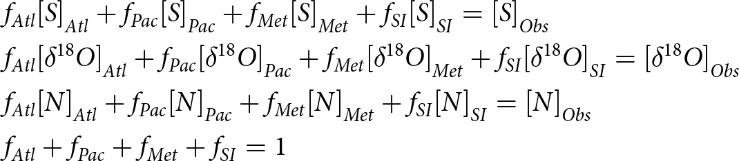(1)\begin{align} \begin{aligned} & {f_{Atl}}{\left[ S \right]_{Atl}} + {f_{Pac}}{\left[ S \right]_{Pac}} + {f_{Met}}{\left[ S \right]_{Met}} + {f_{SI}}{\left[ S \right]_{SI}} = {\left[ S \right]_{Obs}}\\ & {f_{Atl}}{\left[ {\delta {}_{}^{18}O} \right]_{Atl}} + {f_{Pac}}{\left[ {\delta {}_{}^{18}O} \right]_{Pac}} + {f_{Met}}{\left[ {\delta {}_{}^{18}O} \right]_{Met}} + {f_{SI}}{\left[ {\delta {}_{}^{18}O} \right]_{SI}} = {\left[ {\delta {}_{}^{18}O} \right]_{Obs}} \\ & {f_{Atl}}{\left[ N \right]_{Atl}} + {f_{Pac}}{\left[ N \right]_{Pac}} + {f_{Met}}{\left[ N \right]_{Met}} + {f_{SI}}{\left[ N \right]_{SI}} = {\left[ N \right]_{Obs}}\\ & {f_{Atl}} + {f_{Pac}} + {f_{Met}} + {f_{SI}} = 1\end{aligned}\end{align}

where ${f_i}$ is the fraction component in a water parcel and ${\left[ X \right]_i}$ is the property $X$ value for the end member of the individual water components. The four water end members are Atlantic ( $Atl$), Pacific ( $Pac$), meteoric ( $Met$) and sea-ice meltwater ( $SI$). ${\left[ {\delta {}_{}^{18}O} \right]_{SI}}$ is the oxygen isotope anomaly for sea-ice meltwater. It is different from the surface water in which the ice forms because the heavier isotopes of water are incorporated preferentially into the ice. It is this fractionation that we are interested in here, and we view the sea-ice meltwater δ¹⁸O as the sum of the surface water δ¹⁸O value and an offset. ${\left[ {\delta {}_{}^{18}O} \right]_{SI}}$ means δ¹⁸O value for sea-ice meltwater, which is the sum of δ¹⁸O in surface water and δ¹⁸O effective fractionation coefficient between water and sea ice. $S$ is the salinity, $N$ is the nutrient concentration, and $Obs$ means observations for the measurement of a sample and the last equation stands for mass conservation (Östlund and Hut, 1984; Ekwurzel et al., 2001; Newton et al., 2013).

The principal source of error in these equations is the error in our estimation of the end members. H₂¹⁸O is enriched relative to H₂¹⁶O in sea ice during freezing of sea water (Lange et al., 1990). Therefore, to minimize error we have to know the isotope fractionation coefficient for oxygen during the freezing process. Previous estimates of fractionation have been based on either laboratory experiments or natural sea ice (Toyota and 7 others, 2013). However, much interest is in older sea ice, which has traversed long distances and plays a critical role in the Arctic ecology and climate. In what follows, we present a new dataset, collected during one of our ‘Switchyard’ field expeditions for which we have stable isotope measurements on both ice cores and the underlying surface water. From this data, we calculate a new estimate of the oxygen isotope fractionation coefficients based on measurements of multiyear ice, which has traversed the central Arctic Ocean.

2. Data

2.1. Sampling

The ice cores, typically 2 m long, were collected in the Switchyard region of the Arctic Ocean in May of 2012 (Falkner and 6 others, 2005; Tracking Ocean Changes in the Arctic Switchyard – State of the Planet, 2012). Samples were obtained by Twin Otter aircraft landing on level ice, and then drilling ice cores (Smethie et al., 2011). Log entries from the field crew indicate that ice was still growing in the Switchyard area during the sampling period. The concurrent ice growth is also supported by the ice growth model of Section 3, which shows steady growth in the month leading up to sampling. Water samples were obtained at the same stations through a hole drilled nearby. The station locations were organized to form sections extending from the shelf region in the Lincoln Sea into the Makarov and Amundsen Basins (Figures 1 and 2). Where the ocean depth allowed, samples were drawn down to ∼800 m. In this study, we focus on surface ocean water, and so have used the top sample, taken at ∼5 cm below the bottom of the ice.

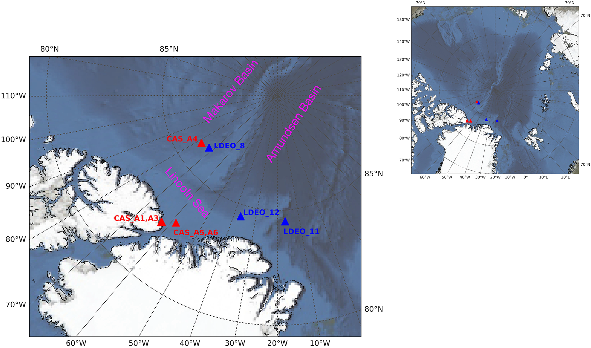
Figure 1. Geographical position of the ice core samples collected in Switchyard. The stations designated by blue triangles were collected by Lamont–Doherty Earth Observatory (LDEO stations) and the stations designated with red triangles were occupied by the Canadian Sea Ice Mass Balance Observatory (CAS stations). Basemap from NASA Blue Marble image (Stöckli et al., 2007).

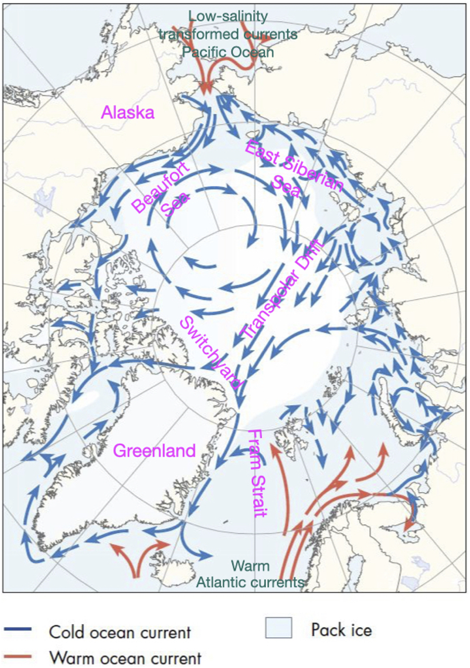
Figure 2. Arctic Ocean surface water circulation schematic, with labels added (Arctic Council, CAFF, Arctic Council, Conservation of Arctic Flora and Fauna Working Group, 2001).

2.2. Data collection and measurement

A steel corer with a plastic liner pipe with cutting knives at the end was used to drill into the ice from the surface to keep the ice core sample intact. After reaching the bottom of the ice, the corer was pulled out of the drill hole, and the ice cores were taken completely, placed into insulating containers and flown to Alert in subzero temperatures (Tracking Ocean Changes in the Arctic Switchyard | Lamont-Doherty Earth Observatory, 2012). The corer was a manual one (Kovacs Enterprise Mark II, driven by two-stroke gas engine). The size (diameter) of the core is 9 cm. Surface ocean water samples were obtained using a novel CTD/rosette system with a narrow diameter to facilitate passage through a 12 in borehole in the sea ice (Smethie et al., 2011). At Alert, they were sectioned into 10 cm vertical sections and then melted in the laboratory. Both the melted sea ice samples and surface water samples were measured with a Picarro cavity ring-down mass spectrometer (CRDS; Walker and 11 others, 2016) in the Lamont–Doherty Environmental Tracer Laboratory. The precision measurement of sea water samples using the CRDS was ±0.03‰ for δ¹⁸O.

Stable isotope data are reported as the per mil deviations of the H₂¹⁸O/H₂¹⁶O ratios from those of Vienna Standard Mean Ocean Water (VSMOW-2) using the δ¹⁸O notation:

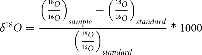(2)\begin{equation}\delta {}_{}^{18}O = {{{{\left( {{{{}_{}^{18}O} \over {{}_{}^{16}O}}} \right)}_{sample}} - {{\left( {{{{}_{}^{18}O} \over {{}_{}^{16}O}}} \right)}_{standard}}} \over {{{\left( {{{{}_{}^{18}O} \over {{}_{}^{16}O}}} \right)}_{standard}}}}*1000\end{equation}

The effective isotope fractionation coefficient (Eicken, 1998; Toyota and 7 others, 2013) is defined as

(3)\begin{equation}{\varepsilon _{eff}} = {\delta ^{18}}{O_{ice}} - {\delta ^{18}}{O_{seawater}}\end{equation}

We take the water immediately below the ice floe as representative of the waters in which the bottom 60 cm of ice has grown. This is, of course, an approximation. Once ice floes are formed, they can travel long distances, sometimes thousands of kilometers, over several years (Pfirman et al., 2004b; Newton et al., 2017). Along the way, they may pass over surface waters with stable isotope compositions quite different from that in their original formation region. Our sampling took place late in the ice formation season, when the bottom of the ice cores is most closely representative of the waters in which the floe has recently resided. In addition, at our stations, the bottom-most 50–70 cm of ice has a relatively uniform δ¹⁸O profile. For these reasons, we therefore believe that our approximation is a good one, and we focus our analysis on comparing the bottom layer of ice with the surface mixed layer samples from the water column at the ice sampling station.

3. Results

To calculate the effective fractionation coefficients, we use the sea water in the surface layer of the ocean for the value of δ¹⁸O sea water. As noted above, this assumes that the water directly below the sea-ice floe is isotopically similar to the water that the ice in the bottommost 0.6 m of the core was formed from. Depth profiles of δ¹⁸O effective fractionation coefficient in this layer are roughly constant (Figure 3). In Canadian Sea Ice Mass Balance Observatory (CAS) stations, the δ¹⁸O effective fractionation coefficient of CAS_A4 is 2.28‰, and that of CAS_A5 is 2.25‰; in Lamont–Doherty Earth Observatory (LDEO) station 8, it is 2.01‰; in LDEO station 11, it is 2.05‰; in LDEO station 12, it is 2.11‰.

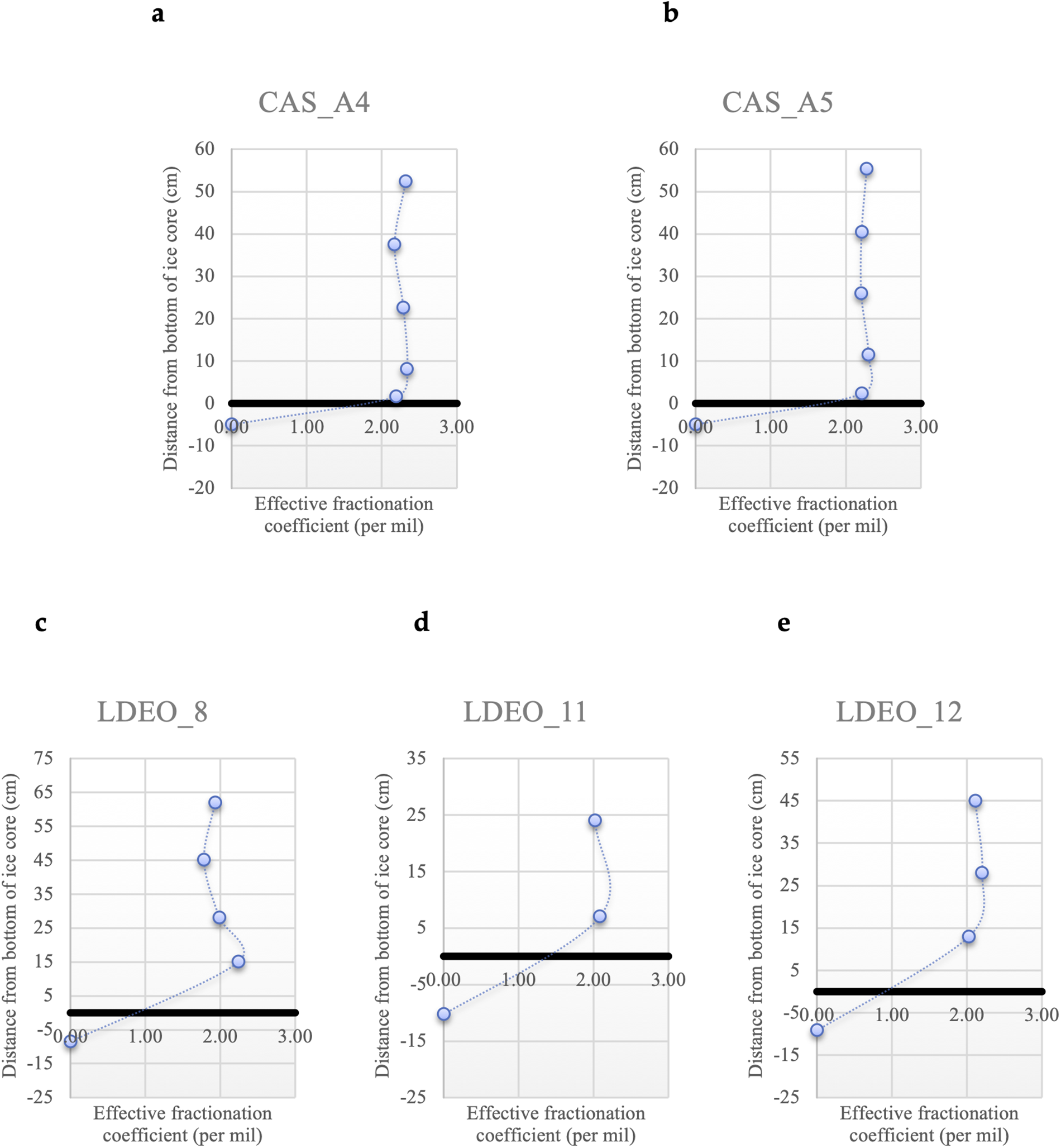
Figure 3. Depth profiles of the effective fractionation coefficients for δ¹⁸O in the bottom 60 cm of the ice core in the Switchyard region. The thick black line is the zero distance from the bottom of the ice core. (a) CAS_A4 station. (b) CAS_A5 station. (c) LDEO_8 station. (d) LDEO_11 station. (e) LDEO_12 station.

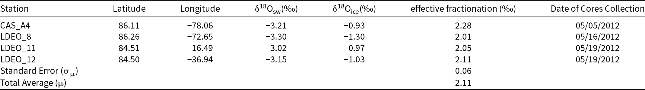
Our ice core sample stations in the Switchyard present different sea ice contexts and expected fractionation coefficients (Figure 1 and Table 1). For CAS stations, CAS_A1 and A3 were from landfast ice which is stationary on the continental shelf (Figure 1). CAS_A5 has almost the same geographic position as CAS_A6, and both of them are also from landfast ice based on Sea Ice Tracking Utility (SITU; Campbell and 6 others, 2019). The effective fractionation coefficient of CAS_A4 from drifting ice shows 2.28‰. For LDEO stations, they are from drifting ice. The effective fractionation coefficients of LDEO_8 and 11 are similar to that of LDEO_12, and the average value of all LDEO stations is 2.06 ± 0.03‰. For all stations in the Switchyard, the average (μ) effective fractionation coefficient is ∼2.17‰ with a standard deviation (σ) value of 0.13‰ and a standard error (σ_μ) of 0.04‰. For stations from drifting ice (CAS_A4 and LDEO_8, 11, 12) in the Switchyard, the average (μ) effective fractionation coefficient provides ∼2.11‰ with a standard deviation (σ) value of 0.12‰ and a standard error (σ_μ) of 0.06‰ (Table 2).

Table 1. Hydrographic data and δ¹⁸O values of ice core samples in the Switchyard region

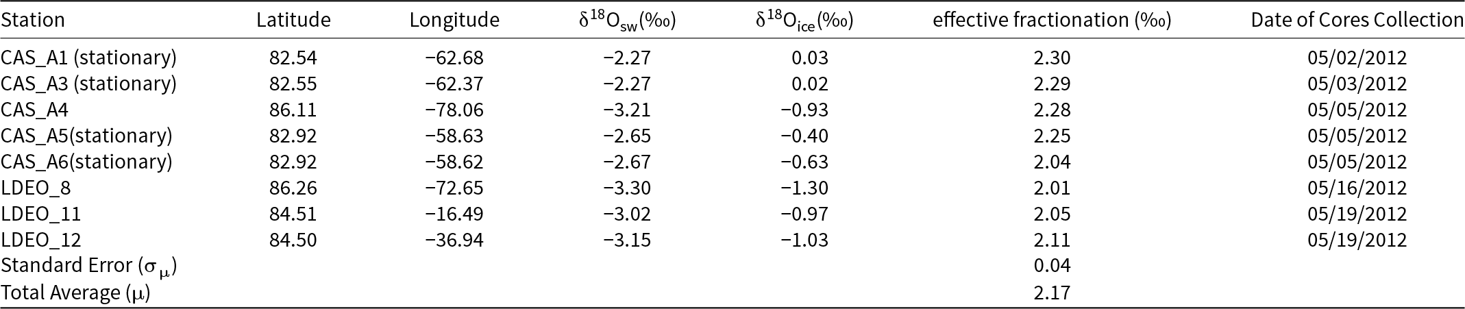
Table 2. Hydrographic data and δ¹⁸O values of ice core samples from drifting ice in the Switchyard region

To better understand the environmental conditions for stations from drifting ice (CAS_A4 and LDEO_8, 11, 12) during sea-ice formation, we used SITU to track sea ice backward in time from our sampling locations to its formation locations (Campbell and 6 others, 2019). Figure 4 shows the sea-ice trajectories tracked back across the Arctic Basin from 1 to 4 years.

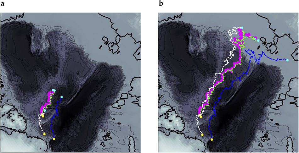
Figure 4. Geographical positions of the ice core stations occupied in the Switchyard region and sea ice back trajectories for CAS_A4, LDEO_8, LDEO_11, and LDEO_12 stations. (a) Back to one year. (b) Back to four years. For all ice core stations, the locations of the ice cores are in yellow and the locations of the ice at earlier times are in cyan. For the tracking lines, CAS station 4 is in magenta, LDEO station 8 in Green, LDEO station 11 in Blue, and LDEO station 12 in White.

SITU also provides data on the environmental conditions along ice trajectories (Campbell and 6 others, 2019), which allows us to investigate the context in which our ice samples in the bottom 60 cm of ice cores formed. Specifically, we can calculate ice growth rates based on the locations along the trajectory where the ice formed, using an ice growth model, together with atmospheric temperature data from SITU. The ice growth model governing equation (Thorndike, 1992; Pfirman et al., 2004a) is

(4)\begin{equation} L*\frac{{\Delta H}}{{\Delta t}} + F + \left( {{T_{IST}} - {T_{ice - water}}} \right)* \frac{{{k_{ice}}*{k_{snow}}}}{{{k_{ice}}*{H_{snow}} + {k_{snow}}*{H_{ice}}}} = 0\end{equation}

where $\frac{{\Delta H}}{{\Delta t}}$ is the ice growth rate, $L$ is the latent heat of fusion, $F$ is the ocean heat flux, ${T_{IST}}$ is the ice surface temperature, ${T_{ice - water}}$ is the ice-water interface temperature, $k$ is the thermal conductivity, ${H_{snow}}$ is the snow thickness and ${H_{ice}}$ is the ice thickness.

We take $L$ = 3 × 10⁸ J (m)⁻³, ${k_{ice}}\,$= 2 W m⁻¹ K⁻¹, ${k_{snow}}$ = 0.33 W m⁻¹ K⁻¹ and ${T_{ice - water}}$= − 1.9 °C (Pfirman et al., 2004a). Due to the simplicity of the selected sea ice model (Thorndike, 1992) and the lack of long-term and Arctic-wide data, for this current study the input of a constant ocean heat flux value was required. We followed previous studies (Maykut and Untersteiner, 1971; Pfirman et al., 2004a; Peeken and 8 others, 2018; Krumpen and 11 others, 2019) and selected a constant ocean heat flux value of $F$ = 2 W m⁻², which was applied to the sea-ice growth model along each trajectory from ice formation to the sampling. We focus on the CAS_A4 station to discuss the ice growth rate along a trajectory, using ${H_{ice}}$=170 cm from our ice core data sets, ${H_{snow}}$= 35.5 cm from the NSIDC database (Canadian Meteorological Centre (CMC) Daily Snow Depth Analysis Data, Version 1, 2021), and ${T_{IST}}\,$ice surface temperature which is close to surface air temperature from SITU (Campbell and 6 others, 2019).

Along the trajectory of CAS_A4 station’s ice floe, we pull back a week at a time, calculate the ice growth rate, save the rate, then multiply that rate by a week’s time, to get each week’s total growth. Then we subtract that total ice growth from ${H_{ice}}$, store the new value at the prior week and take that value as the starting point for the next week back in time. We repeat this loop until the total ice growth is at least 60 cm. For CAS_A4 station, that time was 13 October 2011. Thus, our 60 cm sample grew entirely within the winter prior to our sampling on 5 May 2012. As shown in Figure 4a, the 1 year backtrack shows that our sampled ice grew along a back trajectory extending from the Switchyard approximately to the North Pole. The average estimated ice growth rate along the trajectory was 0.12 mm h⁻¹. To see how sensitive the output of ice growth rate is to snow depth, we also calculate growth using 0.5* ${H_{snow}}$ and 2* ${H_{snow}}$, which gives 0.19 mm h⁻¹ for half snow depth and 0.03 mm h⁻¹for twice snow depth; indicates a standard deviation value of 0.08 and a standard error of 0.05.

We also use the empirical formula by Toyota et al. (2013) and our effective fractionation coefficient to calculate and examine ice growth rate in situ Switchyard conditions. The fitting curve for the symbols of observations presented in Figure 5 overall indicates that the effective coefficient as a function of ice growth rate is reasonable (Figure 5), where the ice growth rate of CAS_A4 station shows 0.24 mm h⁻¹. The ice growth rate 0.24 mm h⁻¹ standing for instantaneous time is larger than that of 0.12 mm h⁻¹ and close to that of 0.19 mm h⁻¹ with half snow depth using observed field thermodynamic balance over previous several months. These results are consistent with those based on our ice growth model.

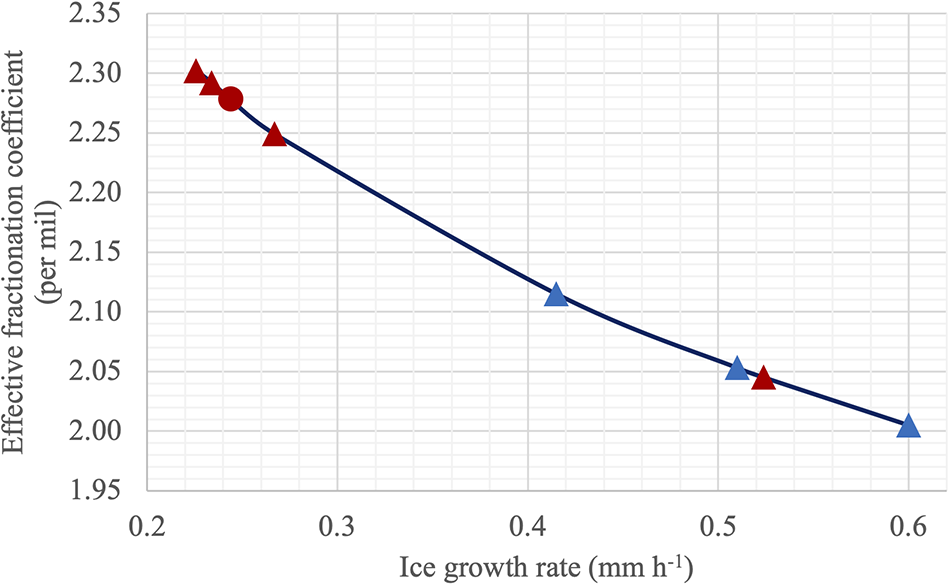
Figure 5. δ¹⁸O effective fractionation coefficient vs ice growth rate in situ Switchyard (CAS stations in red, LDEO stations in blue, CAS_A4 in red solid circle marker).

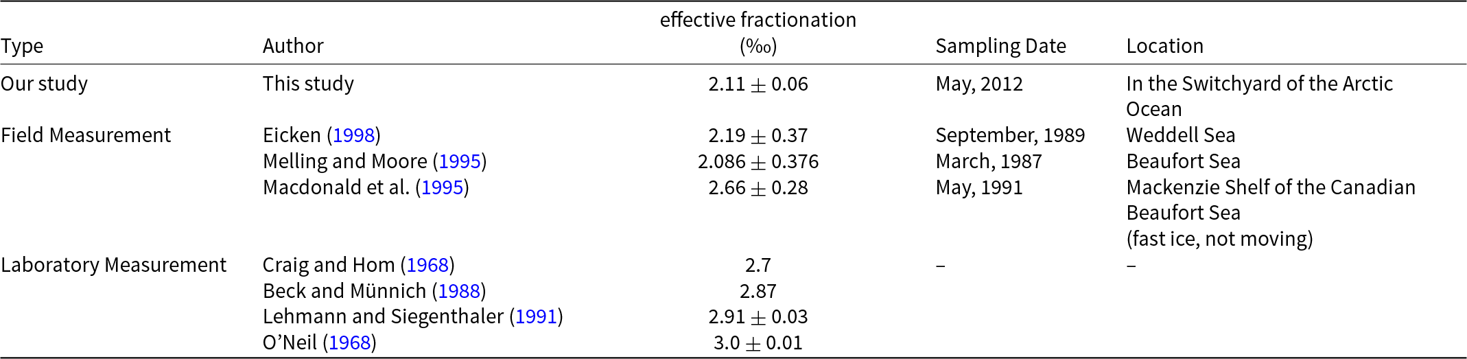
Table 3. Comparison with δ¹⁸O effective fractionation coefficient for field and laboratory measurement in literature

4. Discussion and conclusions

Sea ice context is important in understanding expected fractionation coefficients. Fractionation is known to vary from <0.1‰ for fast-growing (>10 mm h⁻¹) frazil ice up to >2.5‰ for slow-growing (<0.01 mm h⁻¹) columnar ice (Eicken, 1998). The effective oxygen isotope ratio fractionation coefficients between surface water and sea ice in the Arctic Switchyard for drifting ice averages 2.11 ± 0.06‰. As shown in Table 3, this average value is close to the value of 2.19‰ reported in Eicken (1998) for the Weddell Sea, and the value of 2.086‰ reported by Melling and Moore (1995) based on Arctic field measurements. It is somewhat higher than the value of 2.0‰ used by Pfirman et al. (2004a) in their reconstructions of Arctic surface ocean conditions from sea-ice cores. As expected, the value in our field study is significantly lower than the value of 2.66‰ reported in Macdonald et al. (1995)’s Arctic field sampling of landfast ice and the waters below it. Also, our field samples exhibit less fractionation than the ∼2.7–3‰ observed in laboratory measurements (Craig and Hom, 1968; O’Neil, 1968; Beck and Münnich, 1988; Lehmann and Siegenthaler, 1991). Conditions in the field with drifting ice are more dynamic than conditions in the laboratory or under landfast ice, where the water is usually slower-moving than in the open ocean. Rapidly growing sea-ice growth traps brine pockets (Niedrauer and Martin, 1979), which over time may be incorporated into the ice matrix. Maximal fractionation occurs when sea ice forms in isotopic equilibrium with well mixed bulk water by slow freezing. Importantly, some laboratory experiments such as Lehman and Siegenthaler’s are conducted with fresh water. As sea water freezes, high-salinity brines are rejected, forming a dense layer at the ice/ocean interface that results in convection. Convective overturning or rapid freezing makes equilibrium conditions highly unlikely, even in otherwise quiescent conditions. The laboratory experiments represent an approximate upper bound on the fractionation coefficient because they proceed near equilibrium. Field conditions, on the other hand, are highly dynamic, with changing winds, temperatures, as well as under-ice topography and variable ocean turbulence that keep the system far from equilibrium conditions.

The SITU backtracks point to origins in the East Siberian Sea, indicating that these ice floes originated over, or at the edge of, the East Siberian continental shelf. Oxygen isotope ratios in surface waters near the Laptev and East Siberian seas are highly variable, and often well below zero (Bauch and Cherniavskaia, 2018). By the time the ice floes reach the Switchyard, they have been through several seasonal freeze cycles since their initial formation, and the last winter’s conditions are what is imprinted in the lower 60 cm of the ice column. Figure 4a indicates that this lower 60 cm represents only 1 year of growth, between the North Pole and the Switchyard, and within the consistent hydrography of the Transpolar Drift (Pfirman et al., 2004a). This is why the effective fractionation coefficients of the bottom sections of our ice cores are nearly constant with ice core depth in the lowermost layer at all stations.

Furthermore, because the samples were obtained from level ice and were mostly at ice depths more than 1.5 m, the ice likely grew slowly under quiet water conditions not disturbed by nearby under-ice topography. Therefore, the average value of 2.11‰ for drifting ice, which is only a little lower than that for laboratory-grown ice, is consistent with expectations.

The literature indicates that there is no generally applicable fractionation coefficient. Fractionation depends on the sea-ice growth rate and the degree of homogeneity in the immediately underlying water column, both of which will change with the season and the speed of the floe. In this situation, the way forward is through observational case studies. The advantage of the tracer method used here is that it is integrative, so that it applies not just to the instantaneous time and place of sampling, but over the previous several months of sea-ice growth.

These results yield a generalizable field measurement of sea ice-ocean oxygen isotopic fractionation which is needed for the calculation of water mass fractions in the Arctic Ocean. In addition, they help round out our understanding of the way that isotopic fractionation varies depending on conditions. In the most dynamic situations, during the formation of fast-growing frazil ice, extreme cold and high winds, when ice is formed quickly above constantly renewed surface water, fractionations will be lowest. In the most stable conditions, where ice is landfast, and the ice/ocean interface is well-insulated from the atmosphere, ice grows slowly and fractionations can approach laboratory conditions. Our analysis shows that our samples from drifting ice were formed at the bottom of relatively stable thick, multi-year ice floes within the perennial ice pack, flowing over a relatively consistent region of the pelagic Arctic, but subject to small-scale convection and differential flows of sea-ice and the water column. As one would expect, our results are intermediate, between the dynamic Siberian ‘ice factories’ and the highly stable landfast ice areas. We suggest that our results are applicable to multi-year ice throughout the pelagic Arctic.