


1. Introduction
Circular glacier collapse features (from here on referred to as collapse features) are funnel-shaped depressions which typically form on glacier tongues and are associated with circular crevasses. They are hypothesized to be the result of subglacial cavities that grow in size until the overlying ice roof collapses due to mechanical failure (Stocker-Waldhuber and others, Reference Stocker-Waldhuber, Fischer, Keller, Morche and Kuhn2017; Kellerer-Pirklbauer and Kulmer, Reference Kellerer-Pirklbauer and Kulmer2019; Egli and others, Reference Egli, Belotti, Ouvry, Irving and Lane2021). Although these features can be observed on many glaciers in the Alps, relatively little research has been performed on their formation and impact. The frequency at which such collapse features occur was recently shown to have increased in the Swiss Alps since the early 2000s, presumably due to rising air temperatures, glacier thinning and locally decreased ice velocities (Egli and others, Reference Egli, Belotti, Ouvry, Irving and Lane2021). As glaciers around the world—and more particular in the Swiss Alps—continue to experience accelerating mass loss (Zemp and others, Reference Zemp, Gärtner-Roer, Nussbaumer, Welty, Dussaillant and Bannwart2023; GLAMOS, 2024a), collapse features will likely remain a common sight on mountain glaciers. Therefore, where and how such collapse features occur, and which impacts they might have on glacier dynamics and natural hazards, calls for a better understanding of the underlying processes.
The earliest mentions of collapse features or their characteristic circular crevasses in the scientific literature are by King and others Reference King, Emmons and Hague(1871), describing ‘concentric systems of fissures’ on Bolam Glacier at Mt. Shasta (USA) and Srbik Reference Srbik(1937) offering a detailed description of two funnel-shaped collapse features on a dead ice body with ‘radial crevasses’ on Gurglerferner (AUT). Further mentions are by de Boer (Reference de Boer1949); Paige (Reference Paige1956); Loewe (Reference Loewe1957); Morrison (Reference Morrison1958); and Odell Reference Odell(1960). Photographs of some of the earliest documented collapse features are shown by Paige Reference Paige(1956) and Morrison Reference Morrison(1958) on Black Rapids Glacier (USA) and the Homathko Icefield (Canada), respectively. The first mention in the Swiss Alps was on Glacier d’Otemma where a collapse feature is described as a ‘window in the ice’ (Kasser, Reference Kasser1968).
In previous studies, there has been a general consensus that glacier downwasting, low horizontal ice flow velocities preventing closure of the cavity due to ice creep and shallow ice thicknesses are important prerequisites for collapse feature formation (Stocker-Waldhuber and others, Reference Stocker-Waldhuber, Fischer, Keller, Morche and Kuhn2017; Kellerer-Pirklbauer and Kulmer, Reference Kellerer-Pirklbauer and Kulmer2019; Egli and others, Reference Egli, Belotti, Ouvry, Irving and Lane2021). En- and subglacial ablation in form of break-offs of individual ice chunks from the cavity roof (called ‘subglacial stoping’ or ‘block caving’ by Paige, Reference Paige1956) are seen as important mechanisms in enlarging a subglacial cavity, eventually leading to the collapse (Paige, Reference Paige1956; Kellerer-Pirklbauer and Kulmer, Reference Kellerer-Pirklbauer and Kulmer2019; Egli and others, Reference Egli, Belotti, Ouvry, Irving and Lane2021). Ice-marginal streams were first hypothesized to contribute to collapse feature formation by Morrison Reference Morrison(1958), while Kellerer-Pirklbauer and Kulmer Reference Kellerer-Pirklbauer and Kulmer(2019) and Egli and others Reference Egli, Belotti, Ouvry, Irving and Lane2021 mention such streams as an energy source for enhanced basal melt. Stocker-Waldhuber and others Reference Stocker-Waldhuber, Fischer, Keller, Morche and Kuhn(2017) see the importance of ice-marginal streams as a potential supply of sediments which—if deposited at a certain location and later flushed out—could create the initial subglacial cavity required to eventually form a collapse feature. They speculate that sediment evacuation is an important driver of increased subsidence, leading to collapse of the overlying ice. Based on observations from Gepatschferner, Austria, they assume that a sediment layer was flushed out after a strong rainfall event. Egli and others Reference Egli, Belotti, Ouvry, Irving and Lane2021, instead, investigated a collapse feature at Glacier d’Otemma, Switzerland, suggesting the relevance of channel meandering as a mechanism for cavity formation and later collapse, as first described by Paige Reference Paige(1956). A glaciological phenomenon similar to collapse features is ice cauldrons—large shallow depressions on the glacier surface, which form due to a hotspot in basal melt resulting from high geothermal activity (Björnsson, Reference Björnsson2003). While the deformation of the ice and the resulting formation of circular crevasses at the surface are similar to collapse features, ice cauldrons do not collapse, which is why we do not consider them as collapse features in this study. High geothermal activity as a formation mechanism for collapse features is unlikely in Switzerland due to the comparatively low geothermal heat fluxes and the lack of any spatial concentration of such activity (Medici and Rybach, Reference Medici and Rybach1995).
Many important aspects related to collapse features have been identified in previous research, but significant gaps remain in understanding their spatial and temporal distribution, formation and broader implications for glacier dynamics and natural hazards. While Stocker-Waldhuber and others Reference Stocker-Waldhuber, Fischer, Keller, Morche and Kuhn(2017) and Kellerer-Pirklbauer and Kulmer Reference Kellerer-Pirklbauer and Kulmer(2019) provide data from five recent collapse features in Austria, Egli and others Reference Egli, Belotti, Ouvry, Irving and Lane2021 offer a broader overview, analyzing the occurrence of collapse features on 12 Swiss glaciers using observations spanning several decades. A comprehensive inventory of collapse features covering the Alps is, however, still lacking. Furthermore, the contribution of collapse features to ablation and increased glacier retreat has not yet been quantified on the larger scale. At a more fundamental level, there is still limited understanding of the drivers of collapse feature formation and improved comprehension of the relevant processes would advance our understanding of glacier retreat dynamics. Finally, the potential link between collapse features and natural hazards is not well understood, albeit that ‘collapse events’ are suggested to be linked to outburst floods by Swift and others Reference Swift, Tallentire, Farinotti, Cook, Higson and Bryant2021. They hypothesize that due to temporary blockage, subglacial channels could store reasonably large amounts of water, which could then cause a flood upon release of that blockage.
In order to address the above gaps, we establish a Swiss-wide collapse feature inventory using aerial images from 1971 to 2023 and a geospatial machine learning tool. We use this inventory to study the spatial and temporal distribution of collapse features and quantify the contribution of collapse features to overall glacier mass loss at the Swiss scale by leveraging a unique set of temporally repeated, high-resolution digital elevation models (DEMs). To illustrate the drivers responsible for collapse feature formation, finally, we present a case study focused on Rhonegletscher, Switzerland, based on extensive measurements including local glacier mass balance, ice velocities, ground-penetrating radar (GPR) and drone-based DEMs.
2. Data
2.1. Collapse feature detection and glacier mass loss quantification
Collapse features were detected using aerial images provided by the Swiss Federal Office of Topography (swisstopo). The SWISSIMAGE dataset consists of aerial images of Switzerland dating back more than 50 years (swisstopo, 2024c). At the time of the analysis, images from 1971 to 2023 were available. Before 2005, images for any given location in Switzerland were acquired every 6 years with a spatial resolution of 1 m. After 2005, images were taken at 3 year intervals while the resolution increased to 0.1 m since 2017 (swisstopo, 2024c).
To detect collapse features at a higher temporal resolution and in order to quantify mass loss related to collapse features, data from the so-called ‘cryospheric monitoring flights’ (swisstopo, 2024a) were used. The data consist of high-resolution (0.1 m) aerial images and DEMs (spatial resolution of 0.5–1 m), acquired on a yearly basis by swisstopo for a selection of glaciers with detailed monitoring in the frame of the Glacier Monitoring Switzerland (GLAMOS) program. The dataset covers 104 Swiss glaciers over varying time periods between 2011 and 2023. Out of these, 18 glaciers hosted collapse features, 11 of which were covered across their entire lifespan by the cryospheric monitoring flights (Fig. 1).

Figure 1. Glaciers (red dots) used to quantify contribution of collapse features to glacier mass loss in this study. Top-left inset indicates the geographic position of Switzerland (black). Other insets are examples of collapse features at various sites covered by the national cryospheric monitoring flights between 2011 and 2023. North indicated by north arrow. Map data and aerial images by swisstopo (swisstopo, 2024c).
To link individual collapse features to specific glaciers, we use glacier outlines from the Swiss Glacier Inventories (SGIs) for the years 1973 (Müller and others, Reference Müller, Caflisch and Müller1976) and 2016 (Linsbauer and others, Reference Linsbauer2021). The outlines in these datasets were digitized based on aerial images.
In order to analyze the relationship between collapse feature occurrence and ice thickness, we use Swiss-wide ice thickness distributions from Grab and others Reference Grab(2021). This dataset is based on a comprehensive set of GPR surveys, interpolated with two different numerical methods. It provides spatially distributed ice thickness information for any glacier included in the SGI 2016 and has a spatial resolution of 10 m.
To relate mass loss induced by collapse features to overall glacier mass loss, we use annual mass-balance data specified for all individual Swiss glaciers from 1915 to 2023. The corresponding dataset (see Cremona and others, Reference Cremona, Huss, Landmann, Borner and Farinotti2023, for derivation) is based on an extrapolation of in situ measurements collected in the frame of GLAMOS, combined with long-term geodetic mass change (GLAMOS, 2024b).
2.2. Rhonegletscher case study
In order to better understand the formation and evolution of collapse features, we select a collapse feature that existed between 2021 and 2024 at Rhonegletscher as a case study. Various measurements were performed on this feature, including surface and basal mass balance, drone-based DEMs, ground-based GPR and borehole and automatic cameras. An overview of the study site is given in Figure 2 while the acquired datasets are presented in the following.
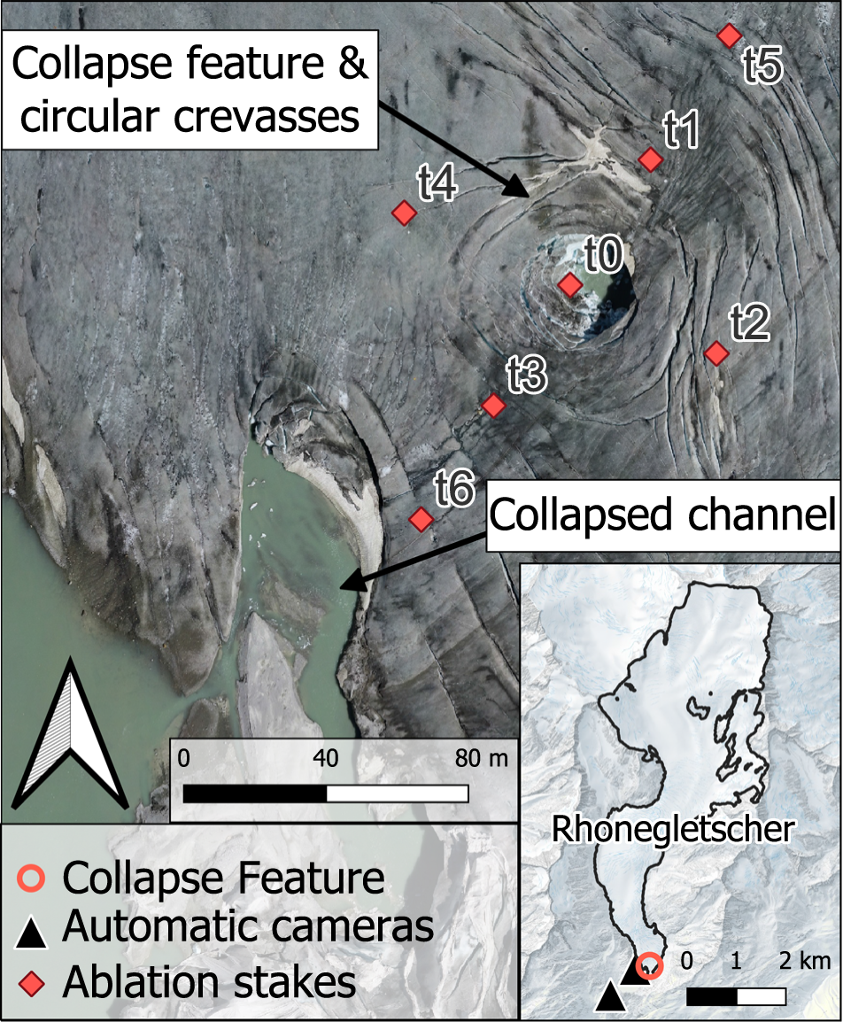
Figure 2. Overview of the study site at Rhonegletscher (see Figure 1 for location). Aerial image from 5 July 2023 showing the collapse feature and a collapsed channel downstream. The locations of the ablation stakes are indicated in red. The inset map depicts the glacier outline (2023) and location of the collapse feature and automatic cameras. North indicated by north arrow.
Glacier-wide mass balance on Rhonegletscher has been measured since 2006, using a network of stakes (GLAMOS, 2024a). In addition to the existing network, ablation stakes were installed at the center of and around the collapse feature in June 2022 and remained there until the fall 2023 (Fig. 2). To monitor ice velocities, including vertical deformation above the subglacial cavity, the stake positions were measured using Global Navigation Satellite System (GNSS). Stake readings and GNSS measurements were conducted every 2 weeks in the melt season of 2022 and sporadically in the melt season of 2023. The central stake was lost in the fall of 2022 as the roof started to partially collapse.
In order to quantify the evolution of the collapse feature and the surface elevation changes, high-resolution DEMs and orthophotos of the glacier terminus were acquired. This was done using a DJI Phantom 4 Pro drone and the surveys were conducted on the same days as the stake readings. The flight height ranged from 50 m to 100 m and the image overlap between consecutive images taken along the same flight path (frontal overlap) was 80% and between images from adjacent flight paths (side overlap) was 70%. The images were processed using ground control points and the software Agisoft Metashape 2.1.3. The resulting horizontal resolution was 20 cm for the DEMs and 10 cm for the orthophotos.
Ice thickness and the subglacial cavity at the center of the collapse feature were measured using ground-based GPR at four different instances throughout the melt season of 2022. GPR was also used to detect the internal structures of the ice, such as the laterally inclined circular crevasses surrounding the collapse feature. The GPR was operated at frequencies of 100 MHz and 250 MHz. The data were processed using the software GPRglaz (e.g. Grab and others, Reference Grab2018) following the processing workflow typically applied to field-based investigations (e.g. Church and others, Reference Church, Bauder, Grab and Maurer2021; Grab and others, Reference Grab2021; Ogier and others, Reference Ogier2023). This workflow comprises (1) time-zero correction based on the arrival of the direct wave, (2) background noise removal, (3) bandpass filtering (filter bounds of 50 MHz to 150 MHz for a central frequency of 100 MHz, and bounds of 200–500 MHz for a central frequency of 250 MHz), (4) traces binning to every 0.5 m or 0.2 m (for 100 MHz and 250 MHz, respectively) and (5) image focusing and time-to-depth conversion that migrates the data with a constant radar wave velocity (0.167 m ns−1 for ice; Glen and Paren, Reference Glen and Paren1975). Migration was performed with a Kirchhoff time-migration scheme (Margrave and Lamoureux, Reference Margrave and Lamoureux2019).
To gain insights into the structure of the subglacial cavity, a borehole was drilled in the center of the collapse feature and a camera was lowered into the cavity. Due to a partial collapse of the cavity roof occurring during the 2022 melt season the borehole was later re-drilled and used to obtain approximate measurements of ice thickness and cavity height. This was done by lowering a weight attached to a rope into the borehole and measuring the rope’s length. Measurements were taken several times throughout the 2022 melt season.
In addition to all of the above, two automatic cameras installed at the glacier’s margin (Fig. 2) captured images of the terminus of Rhonegletscher four times a day (camera 1) and at hourly intervals (camera 2), respectively. The images acquired by these cameras allowed for both monitoring of the collapse feature evolution (e.g. initial roof collapse, melting out of the cavity) and precise determination of the collapse timing.
3. Methods
3.1. Detection of collapse features and inventory creation
To detect collapse features on aerial images between 1971 and 2023, we used a manual approach, aided by an automated pre-screening approach. The overall procedure was to use a set of manually detected collapse features to train the online, geospatial machine-learning tool ‘Picterra’ (Picterra, 2024), which then served as an automated tool to pre-screen aerial images and to locate possible collapse features, which would finally be filtered manually. We initially trained the machine learning algorithm on SWISSIMAGE data from 2011 to 2020. Specific sections of the images were defined as ‘training areas’ and used to outline collapse features that were previously detected manually, i.e. by visual inspection of the images. We chose these training areas to cover a variety of collapse features, including various sizes and appearances (e.g. collapse features occurring on glaciers with differing surface characteristics). The training set consisted of outlines for 139 collapse features. Note that a single collapse feature can be represented by several outlines, as the same feature can appear repeatedly in consecutive aerial images. Based on these outlines, we trained the algorithm to detect collapse features in different settings. Since the algorithm might falsely identify visually similar but unrelated structures as collapse features, we also included areas containing no collapse features in the training set. This was meant to reduce the number of false positives.
To test the automated pre-screening process, we conducted a test-run using aerial images from 2008 to 2010, which were not included in the training set. To reduce processing cost, the 1973 glacier inventory (Müller and others, Reference Müller, Caflisch and Müller1976) was used to exclude non-glaciated terrain—the assumption being that the outlines from 1973 are large enough as to surely include any glacierized area in the test-period (2008–10). To determine the accuracy of the algorithm, we also manually detected collapse features in the same set of aerial images and compared the results to the one from the automated pre-screening process (see Table 1).
Table 1. Results of the test (2008–10) and the full scale (1971–2020) run of the machine learning algorithm. False negatives for full-scale application are an upper-bound estimated from the ratio of false negatives in the test run
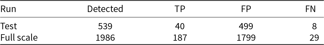
Abbreviations: ‘TP’ = true positive; ‘FP’ = false positive; ‘FN’ = false negative.
The algorithm detected 539 features, most of which (499) were false positives. These were mainly ‘regular’ crevasses and in some cases supraglacial streams or ice cliffs. Although the number of false positives was high, they could be filtered out quickly by visual inspection. While this filtering increased the effort when using the machine learning approach, it remains beneficial compared to manual detection, as it is much easier to manually filter out false positives than trying to visually identify hundreds of collapse features on the large set of aerial images. From the retained features, 40 were true positives while 8 (manually detected) features were not recognized by the machine learning algorithm. Out of these eight false negatives, four features were easier to identify in previous or following years, meaning that they would likely have been detected by the algorithm if using an earlier or later aerial image. The other false negatives were likely too small (∼20 m in diameter) to be detected or underrepresented in the training set (e.g. collapse features on mixed debris-covered/bare ice glaciers).
Following this test, we further trained the algorithm by including the true positives detected in the test run into the training set. In this way, a wider visual variety of collapse features was incorporated. We also included additional training areas containing structures that were previously mistaken for collapse features. Then, we conducted a full-scale run by using the machine learning approach to detect collapse features on aerial images from 1971 to 2007. Due to the high number of false positives (Table 1), we applied manual filtering in the same manner as for the test-run. At the time of this analysis, the 2020 aerial images were the newest available from the SWISSIMAGE data. Collapse features appearing on images obtained after the full-scale machine learning run were inspected visually, and the identified collapse features were manually added to the inventory.
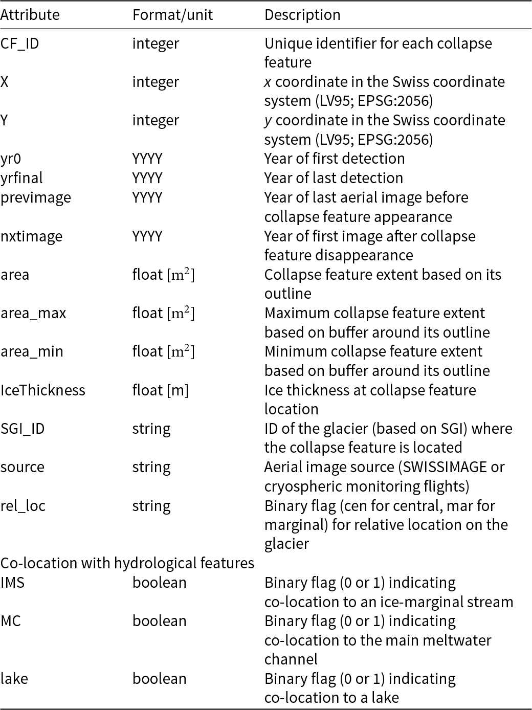
In our inventory, each collapse feature is represented by one entry with the following attributes (Table 2): collapse feature ID, x and y coordinates (LV95 coordinate system), first and last time of appearance (year), previous and subsequent available aerial image (before collapse feature appearance and after end of feature lifespan, respectively), relative location of the collapse feature on the glacier (central or marginal), co-location with glacio-hydraulic components (main meltwater stream, ice-marginal streams and proglacial lakes), collapse feature area (including maximum and minimum extent of the collapse feature), ice thickness (in the year 2016) at the location of the collapse feature (from Grab and others, Reference Grab2021), glacier ID (SGI-ID) and image source (SWISSIMAGE or cryospheric monitoring flights). Pertaining to the relative location of collapse features, features close to the glaciers center line but also to the snout (margin) are classified as ‘central’. To account for uncertainties in the collapse feature area, we set a ±10 m buffer (roughly representing 10% of the average collapse feature diameter) around the collapse feature outline, resulting in a maximum and minimum area value for each collapse feature. The features are outlined by hand, if possible (depending on aerial image availability), at a late stage of their lifespan. This is meant, to account for the widening of the features after the initial roof collapse.
Table 2. Overview of the collapse feature inventory attributes
In order to determine a possible connection to cavity formation by subglacial melt induced by the main meltwater stream, ice-marginal streams or glacial lakes, we investigated the co-location of these hydrological features with the collapse features. We do not consider smaller streams, since we assume they lack the energy to cause sufficient basal melt for inducing a collapse feature. This was done by inspecting aerial images just before or directly after the collapse and identifying any of the features mentioned above. For main meltwater streams, this meant identifying large (pro-)glacial streams flowing through the collapse feature. For ice-marginal streams, we considered any streams entering the glacier within 500 m upstream of the collapse feature as being co-located. The distance of 500 m is somewhat arbitrary and corresponds to a few times the typical collapse-feature diameter that we observe in our inventory. Glacial lakes were considered to be co-located with a collapse feature if they were visible in the center of the collapse feature directly after collapse. Note that all of these criteria assume that the co-located features were situated in the same place when the collapse feature initially formed.
Since thin ice is a potential prerequisite for collapse feature occurrence (e.g. Stocker-Waldhuber and others, Reference Stocker-Waldhuber, Fischer, Keller, Morche and Kuhn2017; Egli and others, Reference Egli, Belotti, Ouvry, Irving and Lane2021), we analyzed the location of the detected collapse features with respect to the local ice thickness (taken from Grab and others, Reference Grab2021, cf. Section 2.1). As the ice thickness information of individual glaciers may have been acquired in a different reference year than when the collapse feature occurred, we corrected the ice thickness values accordingly. We determine an annual glacier-wide distributed surface elevation change rate (dh) by subtracting two DEMs (swisstopo, 2024b) and then multiply dh with the number of years between the collapse feature’s occurrence and the reference year. This yields a thickness change, which is subsequently used to adjust the observed ice thickness. The analysis is limited to collapse features occurring within the spatial extent of the available ice thickness dataset.
To accurately assess the number of collapse features, it is essential to consider two types of observation biases—spatial and temporal—that arise from the spatially and temporally uneven distribution of aerial image acquisitions. Currently, a third of Switzerland is surveyed every year. In years when more glaciated regions are covered, the total imaged glacier area is larger, compared to other years. This leads to a spatial observation bias. Indeed, with more frequent surveys happening now compared to before 2005, the chances of detecting collapse features are higher. If the acquisition interval is longer than the collapse feature lifespan, moreover, there is a chance that some features might be missed entirely. This is especially relevant for images before 2005 and leads to an additional, temporal observation bias.
To determine the magnitude of the spatial observation bias, we computed the ratio between the number of detected collapse features and the glacier area that is annually covered by aerial images. We normalized the ratio with a value of one indicating a high number of collapse features observed across relatively little glacier area and a value close to zero indicating few collapse features observed across a larger glacier area. This ratio and how it changes over time is meant to indicate qualitatively whether the observed trends in collapse feature count still persist. To correct for the temporal bias, we estimated the number of potentially missed features. This was done by calculating the probability  $P_\mathrm{m}$ of missing a collapse feature as
 \begin{align}
P_\mathrm{m} &= \frac{t_\mathrm{a} - L_\mathrm{avg}}{t_\mathrm{a}},
\end{align}
\begin{align}
P_\mathrm{m} &= \frac{t_\mathrm{a} - L_\mathrm{avg}}{t_\mathrm{a}},
\end{align} where  $t_\mathrm{a}$ is the acquisition interval of the aerial images and $L_\mathrm{avg}$ the average lifespan of a collapse feature. The average lifespan is used as the full distribution of collapse feature lifespans is not known. Based on this probability, a correction factor κ can be calculated as
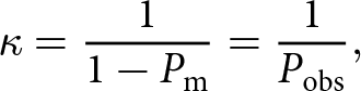 \begin{align}
\kappa &= \frac{1}{1-P_\mathrm{m}} = \frac{1}{P_\mathrm{obs}},
\end{align}
\begin{align}
\kappa &= \frac{1}{1-P_\mathrm{m}} = \frac{1}{P_\mathrm{obs}},
\end{align} where  $P_\mathrm{obs}$ is the probability of observing an actually occurring collapse feature. Using the correction factor, the true number of collapse features (i.e. both missed and observed) can be calculated as
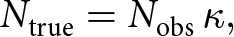 \begin{align}
N_\mathrm{true} &= N_\mathrm{obs} \, \kappa ,
\end{align}
\begin{align}
N_\mathrm{true} &= N_\mathrm{obs} \, \kappa ,
\end{align} where  $N_\mathrm{true}$ and $N_\mathrm{obs}$ are the true and the observed number of collapse features, respectively. Assuming common drivers for collapse feature occurrence, the true number of collapse features in a given year scales with the number of observed features and the area share surveyed in that year (accounted for by κ). The correction factor is thus applied individually to the annual collapse feature count.
The increasing resolution of aerial images over the years (from 1 m in 1971 to 0.1 m at present) could also lead to an observation bias, since collapse feature detection is facilitated by higher resolution. However, based on the size of collapse features and their associated structures—such as circular crevasses and collapsed ice roofs—that are both at least one order of magnitude larger than the image resolution, we do not suspect the change in resolution to have affected collapse feature detection.
3.2. Ablation due to collapse features
The ice loss related to collapse features is the sum of internal and basal (subsurface) ablation. Surface melt is also expected to occur in the area of the collapse feature but is not a result of the collapse feature’s presence as such. In the short term, subsurface ablation can create subglacial cavities, but in the long term, it will result in vertical ice motion related to cavity closure or collapse. We can thus estimate vertical ice motion due to cavities by subtracting (i) the ice surface lowering rate in regions not impacted by the collapse feature from (ii) the surface lowering rate observed in the area of the feature (Fig. 3). By integrating vertical ice motion over the entire lifespan of a collapse feature, the subsurface ablation induced by the collapse can then be determined.
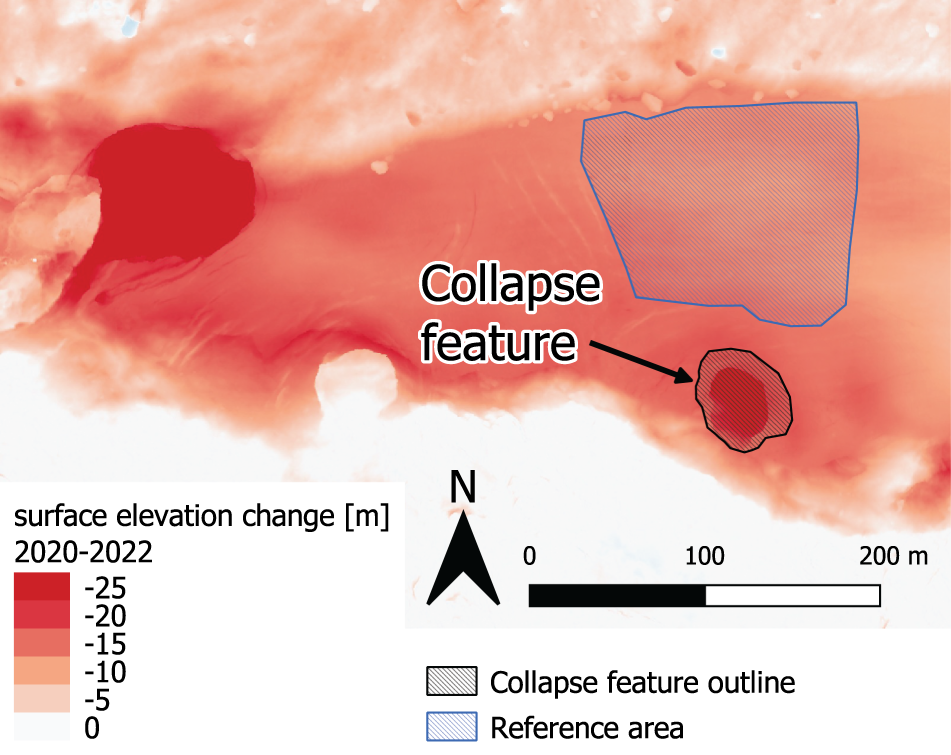
Figure 3. Example from Findelgletscher (see Figure 1 for location) illustrating how the collapse feature and a reference area are mapped on the DEM difference. Both the collapse feature (black) and the reference area (blue) are manually outlined. Subtracting the elevation change within the collapse feature from the one of the reference area yields the subsurface ablation related to the collapse feature. North indicated by north arrow.
For determining the surface elevation change rates, we use DEM differencing of the cryospheric monitoring flights. DEM differencing also proved useful for detecting the exact onset of collapse feature formation, since the locally increased vertical ice motion often appears before the formation of circular crevasses (Fig. 3). We determined surface lowering using a manually assigned reference area outside the collapse feature and on the same elevation band. We then computed vertical ice motion within the area of the collapse feature by subtracting the reference surface elevation change outside of the feature from the surface elevation change within the feature. A similar approach is used in Antarctic subglacial lake research (e.g. Siegfried and Fricker, Reference Siegfried and Fricker2018). Using the vertical ice motion over time and an outline of the specific collapse feature, we determined the ice volume lost due to subsurface ablation. Note that the ice volume loss computed in this way is not necessarily related to the volume of the subglacial cavity, but rather a function of cavity area, rate of subsurface ablation and duration of cavity presence.
In order to estimate the Swiss-wide ice loss for all observed collapse features, an upscaling is needed. This is achieved by establishing a relationship of the form  $V = k\,A^\gamma$ (Bahr and others, Reference Bahr, Meier and Peckham1997) between collapse feature area A and ice loss volume V for the features identified in the annual cryospheric monitoring flights. The relationship includes a scaling factor k and—due to the assumed nonlinear nature of the relation—an exponent γ. We assume a nonlinear relation because the shape of a collapse feature tends to be one of a hemisphere rather than a cuboid. We then applied this empirical relationship to all observed collapse features listed in the inventory, yielding the estimated subsurface ablation caused by each observed collapse feature. To compare the ablation caused by any collapse feature occurring on any glacier, to overall mass balance of that glacier, first the cumulative glacier-specific mass change (using data from
GLAMOS, 2024b) over the entire lifespan of the collapse feature was calculated as
$V = k\,A^\gamma$ (Bahr and others, Reference Bahr, Meier and Peckham1997) between collapse feature area A and ice loss volume V for the features identified in the annual cryospheric monitoring flights. The relationship includes a scaling factor k and—due to the assumed nonlinear nature of the relation—an exponent γ. We assume a nonlinear relation because the shape of a collapse feature tends to be one of a hemisphere rather than a cuboid. We then applied this empirical relationship to all observed collapse features listed in the inventory, yielding the estimated subsurface ablation caused by each observed collapse feature. To compare the ablation caused by any collapse feature occurring on any glacier, to overall mass balance of that glacier, first the cumulative glacier-specific mass change (using data from
GLAMOS, 2024b) over the entire lifespan of the collapse feature was calculated as
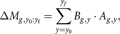 \begin{align}
\Delta M_{g,y_0:y_{\mathrm{f}}} = \sum_{y=y_0}^{y_f} B_{g,y} \cdot A_{g,y},
\end{align}
\begin{align}
\Delta M_{g,y_0:y_{\mathrm{f}}} = \sum_{y=y_0}^{y_f} B_{g,y} \cdot A_{g,y},
\end{align} where  $\Delta M_{g,y_0:y_{\mathrm{f}}}$ is the cumulative mass change of glacier g over the entire collapse feature lifespan, y 0 is the year the collapse feature is first observed, $y_\mathrm{f}$ is the final year the collapse feature is observed, and $B_{g,y}$ is the mass balance of glacier g in year y and $A_{g,y}$ is the corresponding area. The relative contribution $C_{i,g}$ of ablation induced by a specific collapse feature i to cumulative mass change of the respective glacier g can then be calculated as
 \begin{align}
C_{i,g} &= (a_{i,g}\cdot \frac{\rho_\mathrm{ice}}{\rho_\mathrm{water}})\big/\Delta M_{g,y_0:y_{\mathrm{f}}} \cdot \,100\% ,
\end{align}
\begin{align}
C_{i,g} &= (a_{i,g}\cdot \frac{\rho_\mathrm{ice}}{\rho_\mathrm{water}})\big/\Delta M_{g,y_0:y_{\mathrm{f}}} \cdot \,100\% ,
\end{align} where  $a_{i,g}\cdot \frac{\rho_\mathrm{ice}}{\rho_\mathrm{water}}$ is the mass loss caused by collapse feature i, $\rho_\mathrm{ice}$ and $\rho_\mathrm{water}$ the densities of ice and water, respectively. We calculate $C_{i,g}$ for all collapse features in our inventory.
Furthermore, we evaluate the contribution of all observed collapse features to total mass change of all Swiss glaciers for a specific time period as
 \begin{align}
C_{\mathrm{reg},t_0-t_1} = (\sum_{i=1}^{n} a_{i,t_0-t_1}\cdot \frac{\rho_\mathrm{ice}}{\rho_\mathrm{water}})\big/\Delta M_{\mathrm{reg},t_0-t_1} \cdot \,100\% ,
\end{align}
\begin{align}
C_{\mathrm{reg},t_0-t_1} = (\sum_{i=1}^{n} a_{i,t_0-t_1}\cdot \frac{\rho_\mathrm{ice}}{\rho_\mathrm{water}})\big/\Delta M_{\mathrm{reg},t_0-t_1} \cdot \,100\% ,
\end{align} where  $C_{\mathrm{reg},t_0-t_1}$ is the regional relative contribution of ablation induced by collapse features to Swiss-wide cumulative mass change in the time period t 0 to t 1, $\sum_{i=1}^{n} a_{i,t_0-t_1}$ is the total ablation of all collapse features i = 1 to i = n occurring in the time period t 0 to t 1 and $\Delta M_{\mathrm{reg},t_0-t_1}$ is the Swiss-wide cumulative mass change in the respective time period.
4. Results
4.1. A Swiss inventory of glacier collapse features
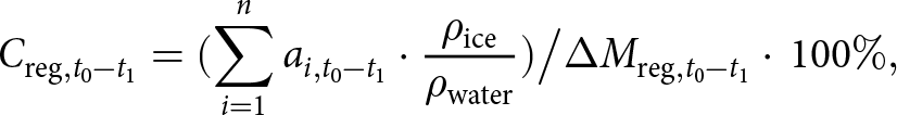
Between 1971 and 2023, we detected 223 collapse features located on 77 different glaciers (Fig. 4). This means that most of the 1400 Swiss glaciers did not host a collapse feature in the last 50 years. Forty-seven out of the seventy-seven glaciers hosted more than one collapse feature, with 30% (=23) of the glaciers hosting 60% (=137) of all observed features. 153 (69%) collapse features were in a central position on the glacier while 60 (27%) collapse features were located close to the glacier margin. In only a few cases, feature location did not fit either of these criteria, being distributed somewhere between the center line and the margin of the glacier, usually on smaller ( $ \lt 1\,\mathrm{km}^{2}$) glaciers or dead-ice bodies (e.g. tongue of Wildstrubelgletscher, see Fig. 1). 46% of the features were co-located with the main meltwater stream, 39% of the features were positioned where an ice-marginal stream enters the glacier and 19% of the features were co-located with a glacial lake appearing during the collapse (e.g. Chessjengletscher in 2023, see Fig. 1). There were only nine collapse features where neither a main meltwater stream, nor an ice-marginal stream, nor a lake was co-located. Based on our observations, we cannot assess with certainty whether a stream or lake was present at the time of formation of these nine collapse features. However, if one of these was present, it must have disappeared before the collapse feature melted out.
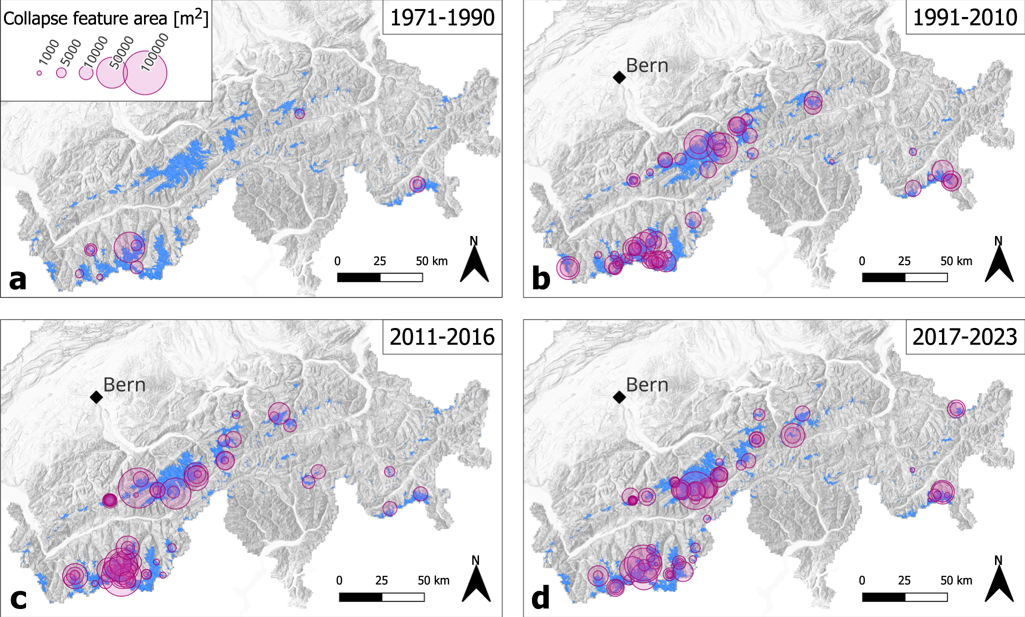
Figure 4. Spatial distribution of collapse features in the Swiss Alps. The collapse feature area is displayed with circles of relative size (see legend). The four panels show four different time periods between 1971 and 2023. Note that panels a and b show 20 year time periods while panels c and d show 5 year time periods. Collapse features are shown in the panel corresponding to the time period in which they were first observed. Glacier extent (SGI 2016) is shown in blue. North indicated by north arrow. Map data by swisstopo (swisstopo, 2024b).
Collapse feature area varies between  $700\,\mathrm{m}^{2}$ and $83\,400\,\mathrm{m}^{2}$, with an average of $12\,600\,\mathrm{m}^{2}$ ( $-3500/+4100\,\mathrm{m}^{2}$) and a median of $8600\,\mathrm{m}^{2}$ ( $-3100/+3800\,\mathrm{m}^{2}$; Fig. 5). There is a wide distribution of sizes, with the largest features reaching up to 370 m in diameter. The largest features are found on large valley glaciers (glacier area $ \gt 6\,\mathrm{km}^{2}$), often spanning a considerable portion of their width (up to half the width in some cases). Forty-five out of the fifty largest features (all $ \gt 16\,700\,\mathrm{m}^{2}$) appeared on the terminus of a valley glacier with a distinct glacier tongue. The other five of the fifty largest collapse features occurred on smaller glaciers ranging in size between $1.2\,\mathrm{km}^{2}$ and $2.2\,\mathrm{km}^{2}$. Most of the small features (21 out of the 30 smallest, all $ \lt 2700\,\mathrm{m}^{2}$) appeared on glaciers smaller than $2.5\,\mathrm{km}^{2}$. While there seems to be a connection between collapse feature area and glacier area, it only holds for the smaller (< $2700\,\mathrm{m}^{2}$) and larger ( $ \gt 16\,700\,\mathrm{m}^{2}$) collapse features. Most mid-sized collapse features ranging in area between 3000 and $16\,000\,\mathrm{m}^{2}$ show a large spread in corresponding glacier area (<1 to >40 $\mathrm{km}^{2}$). Collapse feature area, on average, is higher for features located centrally on the glacier (average: $13\,400\,\mathrm{m}^{2}$) compared to features located at the glaciers margin (average: $11\,900\,\mathrm{m}^{2}$).

Figure 5. Area of collapse features plotted against the area of their respective ‘host-glacier’ in the year of their first appearance.
The lifespan of collapse features can vary widely, between 1 and 28 years in our inventory, with a median of 4 years. In the inventory, two collapse features formed before 1971 while 60 features were still present in the latest aerial images (year 2024). These 62 features were, therefore, not considered in this analysis. The determined lifespan is associated with uncertainties, as the SWISSIMAGE aerial images for any given location are usually 3 or more years apart, meaning that shorter-lived collapse features could be missed. When considering exclusively the inventory entries based on the cryospheric monitoring flights (which have yearly acquisitions), the median is 5 years. On average, the collapse feature lifespan is shorter for features located centrally on the glacier (5.4 years) compared to features at the glacier margin (6.0 years). Ninety percent of collapse features with a lifespan of 1 year had a below-average area when compared to the full inventory. However, the longest-lived features were not always among the largest. Out of the five longest-lived features (lasting between 18 and 28 years), four appeared on debris-covered glaciers. We suspect that the debris-covered surface and its resulting reduction in surface melt may have extended their lifespan. We assume that subsurface melt is connected to surface melt rates in part through potential energy production of subglacial meltwater (see Section 5.1; Oerlemans, Reference Oerlemans2013). Additionally, reduced surface melt also means a reduction in cavity-roof thinning and delayed mechanical collapse of the roof. The five longest-lived collapse features all appeared before 1994 and most occurred on glaciers with relatively limited frontal retreat. The longest-lived feature was first observed in an aerial image of 1993 and was located on the tongue of Rossbodegletscher. We attribute the longevity of this particular feature to frequent avalanching into the feature, reducing ablation rates, thus potentially delaying collapse (Supplementary Fig. S1).
Collapse features were present throughout the entire observation period (1971–2023), with a marked increase since the early 2000s (Fig. 6a and b). 90% (201 features) of the 223 collapse features in the inventory appeared after 2000 and 74% (164 features) after 2010. Figure 6b shows the number of observed collapse features in any given year. Since the increase in detected collapse feature count coincides with the change in acquisition interval of aerial images in the year 2005, the increase could potentially be related to observation biases. Given the acquisition interval of aerial images of 6 years (before 2005) and the average collapse feature lifespan of 4.4 years, we determine the probability of missing a collapse feature before 2005 to be 0.27 (Eqn (1)). Given a correction factor κ of 1.37 (Eqn (2)) and the number of observed collapse features from before 2005 (30 collapse features), we estimate the number of missed collapse features to be 11 (Fig. 6a). We, therefore, assume that the change in acquisition interval from 6 years to 3 does not significantly alter the observed trend in collapse feature appearance. Note that, due to our methodology (Section 3.2), this correction is applied only to collapse features that appeared before 2005. However, we deem this approach sufficient, as any missed features after 2005 would only amplify the observed trend of increasing collapse feature occurrences in the early 2000s. When accounting for the spatial bias, the change in the overall trend is also minimal (Fig. 6c). We thus argue that the increase observed in the early 2000s must be an actual signal.
Figure 6. Temporal distribution of collapse features on Swiss glaciers. (a) Count of newly appearing collapse features between 1971 and 2023. An estimate for the missed collapse features before 2005 (light blue) is provided based on the difference between average collapse feature lifespan and aerial image acquisition interval (Section 3.1; Equations (1)–(2)). (b) Number of observed collapse features visible at any given point in time. (c) Normalized ratio of newly appearing collapse features and glacier area covered by aerial images in that particular year. A value of 1 indicates a high number of collapse features observed across a relatively small glacier area, and a value close to 0 indicating a low number of collapse feature observed across a relatively large glacier area.
The ice thickness at the location of the 133 collapse features identified in our inventory is positively correlated with collapse feature area, with larger collapse features occurring in areas with thicker ice (Fig. 7a). The maximum estimated ice thickness associated with a collapse feature was 128 m and was found at the terminus of Fieschergletscher (Fig. 7b). This particular feature does seem to be an outlier in the sense that it occurs in much thicker ice than most other features and that it does not follow the same trend between ice thickness and collapse feature area as other features. We assume that this may be due to the complexity of this specific collapse feature and glacier terminus (see supplementary Fig. S2), which might have impacted the accuracy of the ice thickness measurements. Additionally, there are a few very large features which seem to occur in relatively thin ice (Fig. 7a). While a clear cutoff is not visible, most features occur in areas of thin ice, with 90% of the analyzed collapse features occurring in places with an ice thickness of 76 m or less and 50% of the collapse features with a thickness of 31 m or less. For comparison, the 90th and 50th percentiles of the mean ice thickness of all glaciers hosting collapse features are 181 m and 53 m, respectively. If collapse feature occurrence were independent of ice thickness, their distribution would approximately follow the ice thickness distribution of glaciers in general. However, the concentration of collapse features in thinner ice indicates that below-average ice thickness is an important prerequisite for collapse feature formation. This strengthens the hypothesis that increased glacier thinning could lead to increased collapse feature appearance, as this particular prerequisite for collapse features is more likely to be met. More specifically, our observations indicate that a local thinning below a thickness of ca. 76 m is a necessary (but not sufficient) condition for collapse features to form (Fig. 7). Our data indicate that collapse feature-associated ice thickness and lifespan do not seem to correlate. Furthermore, even when considering variations in surface melt rates—which might be expected to influence feature longevity through increased cavity roof thinning—no clear pattern emerges. This suggests that, relative to subsurface melt, surface melt plays a minor role in determining collapse feature lifespan.
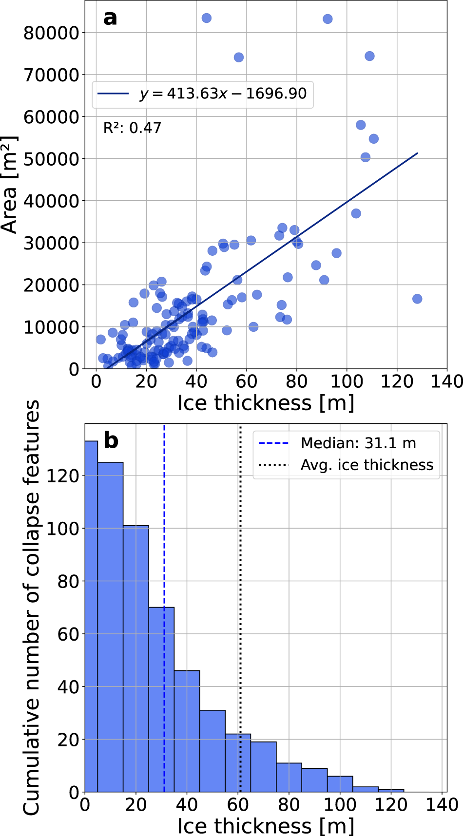
Figure 7. (a) Correlation between local glacier thickness (Grab and others, Reference Grab2021) and collapse feature area for n = 133 cases. The linear fit achieves an R 2 of 0.47. (b) The cumulative number of collapse features that have occurred at ice thicknesses greater than or equal to the corresponding x-axis value. The median ice thickness at collapse features locations (dashed vertical line) and the average thickness of all Swiss glaciers (dotted) are shown as reference.
4.2. Ice loss volume of collapse features
Thirty-two collapse features were analyzed using the DEMs derived from the cryospheric monitoring flights allowing determination of the corresponding ice volume loss. Volume losses of between 1100 and  $445\,000\,\mathrm{m}^{3}$ with an average value of $56\,700\,\mathrm{m}^{3}$ and a median value of $25\,200\,\mathrm{m}^{3}$ were found. Ice volume loss and area of collapse features are positively correlated. They follow a nonlinear relationship and are, therefore, plotted in a log-log space (R 2 = 0.63; Fig. 8). A regression analysis between collapse feature area (A) and volume (V) yields the relation $V = 0.57 \, A^{1.25}$, the exponent of 1.25 indicating that the relation is nonlinear.
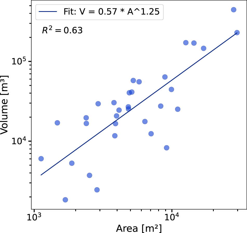
Figure 8. Power-law relationship between area and volume of collapse features analyzed between 2012 and 2023 based on data of the cryospheric monitoring flights (n = 32).
By applying this scaling relation to all collapse features in the inventory, we estimate the volumetric ice loss induced by all observed collapse features between 1971 and 2023 to be  $19.8\times 10^6\,\text{m}^3$ of ice (confidence interval derived from the assumed uncertainty in area (see Section 3.1) $= [13.8 , 27.3]\times10^6\,\mathrm{m}^3$). Note that we only consider observed collapse features and not the estimated true number of collapse features (Fig. 6), since we lack information about the area of those missed features and therefore cannot estimate their ice loss volumes. Relative contributions of individual collapse features to the total mass loss of the respective glacier (Section 3.2) ranged from almost 0 to almost 9%. The maximal value of 8.9% refers to Chilchalpgletscher, a very small glacier (area: $0.05\,\mathrm{km}^{2}$) that had a collapse feature covering as much as 20% of its surface in the year 2015. Over the entire observation period (1971–2023), collapse features contributed only 0.038% to mass loss of all Swiss glaciers. This relative contribution has, however, substantially increased over time from 0.003% (1971–2000) to 0.099% (2011–23). The three glaciers with the highest volume loss due to collapse features all hosted multiple collapse features. For Glacier de Zinal with eight collapse features, a volume loss of $2.5\times10^6\,\text{m}^3-0.5/+0.6\times10^6\,\text{m}^3$ was found, for Zmuttgletscher $1.7\times10^6\,\text{m}^3-0.3/+0.4\times10^6\,\text{m}^3$ distributed over six features and for Mittelaletschgletscher $1.0\times10^6\,\text{m}^3-0.2/+0.3\times10^6\,\text{m}^3$ for five features. Overall, these numbers show that albeit important, the process of collapse feature formation is unlikely to dominate the mass balance of an entire glacier, apart from a fraction of up to a few percent for individual, small glaciers.
4.3. Case study: Rhonegletscher collapse feature
The measurements conducted at Rhonegletscher (see Table A1 in the appendix for an overview) allow us to characterize the life cycle of a collapse feature in detail. First signs of increased surface elevation change between 2020 and 2021 were observed using DEMs. Circular crevasses were first observed during a field visit on 27 October 2021 (Fig. 9) and the ice roof collapsed on 27 June 2023. The collapse feature melted out in the summer of 2024, merging with Rhonegletscher’s proglacial lake and forming the new glacier front. The collapse feature thus lasted ∼2.5 years, from the end of 2021 to summer 2024, making it a relatively short-lived feature compared to the median lifespan in our collapse feature inventory (4 years). After the collapse of the ice roof, the diameter of the feature (including circular crevasses) was roughly 65 m with an area of  $3500\,\mathrm{m}^{2}$. This made it one of the smaller features in the collapse feature inventory (median area: $8600\,\mathrm{m}^{2}$).@@
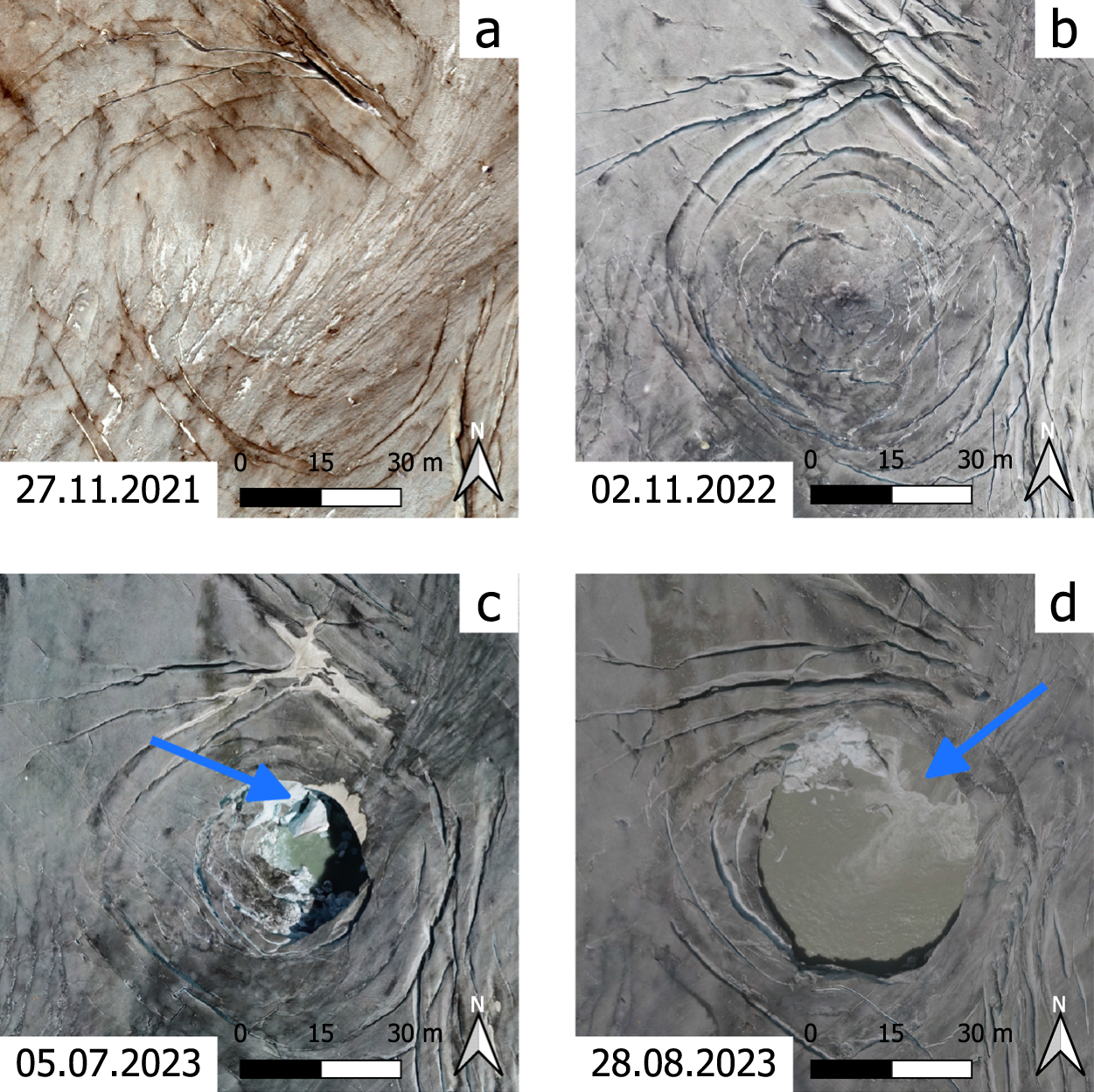
Figure 9. Orthophotos showing the evolution of a collapse feature at Rhonegletscher between late 2021 and 2023. North indicated by north arrow. (a) First signs of circular crevasses. (b) Existing crevasses open up, new ones appear. (c) First image after the ice roof collapse; note the ice blocks indicating subglacial stoping or block caving (arrow). (d) More advanced collapse stage; note the step in the bedrock (arrow).
The presence of a large subglacial cavity at the center of the collapse feature was confirmed by visual inspection through a borehole (14 July 2022; see supplementary material) and by GPR measurements (28 July 2022; Fig. 10). The main meltwater channel could be seen flowing over a bedrock step into the center of the cavity, creating marked turbulence. Also, large ice blocks, likely broken-off lamellas from the ice roof, were seen on the cavity floor. Using the boreholes, the cavity height and the ice roof thickness could be determined. On 14 July 2022, the maximum cavity height ranged from 8.4 to 9.9 m, with a roof thickness of between 14.1 and 13.3 m. The glacier surface was thus between 22.5 and 23.2 m above the cavity floor. We used the GPR derived cavity roof and bedrock elevation do determine the cavity volume at the time of observation. To determine the uncertainty within this volume estimate, we applied the frequency-dependence vertical resolution plus the error in bed elevation (derived from the borehole measurement) to all roof height measurements. We thus obtained a upper (lower) bound for roof elevation and thus a upper (and lower) bound for cavity volume. The GPR-based cavity volume ranged from  $6090\,\mathrm{m}^{3}$ (± $2030\,\mathrm{m}^{3}$) on 28 July 2022 to a maximum of $22\,980\,\mathrm{m}^{3}$ ( $\pm 2740\,\mathrm{m}^{3}$) on 25 August 2022. It decreased to $14\,970\,\mathrm{m}^{3}$ ( $\pm 2210\,\mathrm{m}^{3}$) by 6 October 2022 (Fig. 11).
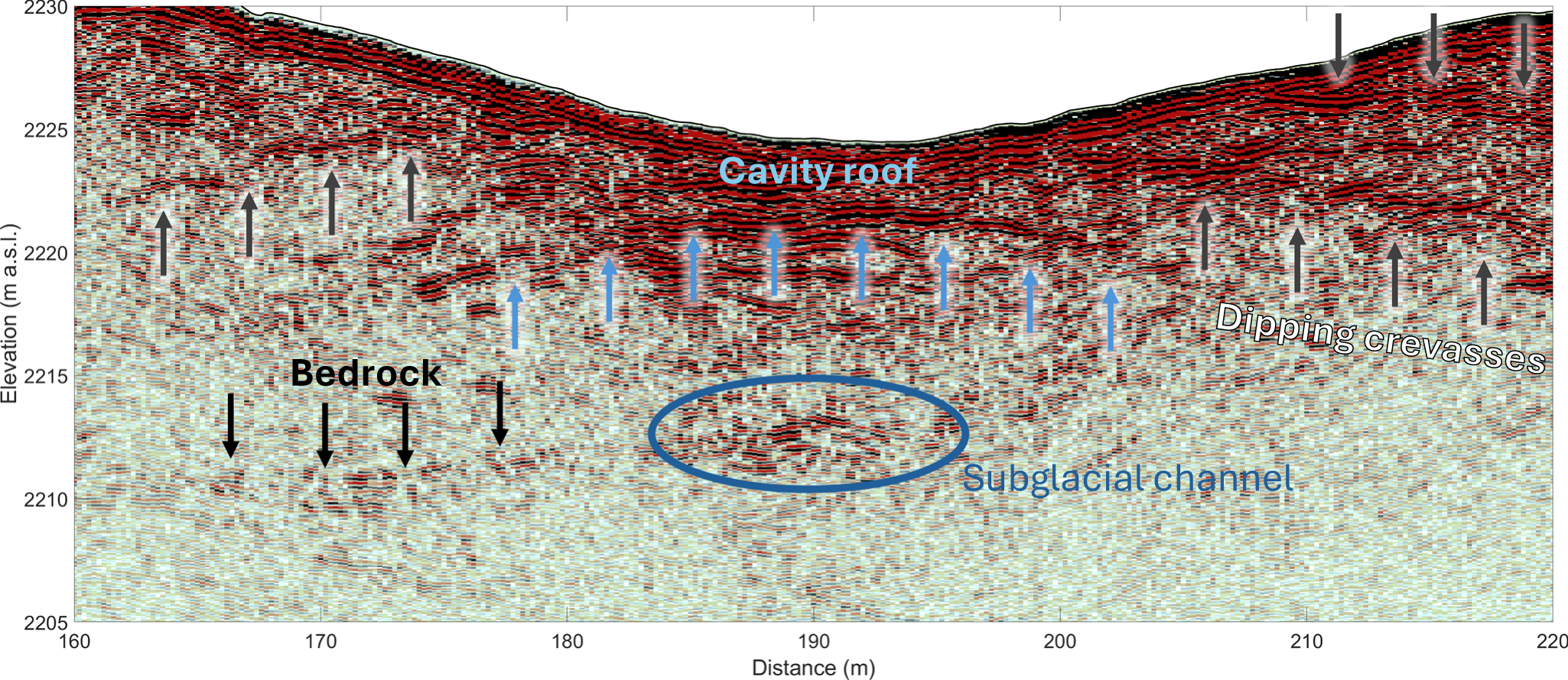
Figure 10. GPR profile of the subglacial cavity at Rhonegletscher, acquired on 7 October 2022. The cavity roof (blue arrows) and dipping crevasses to both sides of the cavity (dark gray arrows) are indicated. The reflection from the subglacial channel is circled in blue. A possible reflection from the bedrock (black arrows) is indicated on the lower left of the figure.
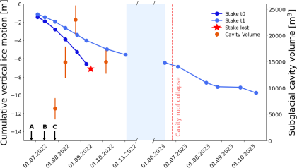
Figure 11. Observations of vertical ice motion (blue dots and lines) and cavity volume (orange dots with error bars) for the collapse feature at Rhonegletscher. The cavity volume was estimated by using GPR-derived bedrock and cavity roof elevation. The red dashed line indicates the time of the cavity roof collapse. The blue shading indicates an observation-break over winter. Labels on the time axis: A: Start of regular field visits. B: Boreholes drilled into cavity. C: Collapse of the subglacial stream downstream of the collapse feature. For more details, see Table A1.
By subtracting the surface melt measured at our stakes surrounding the collapse feature (Fig. 2) from the changes in ice roof thickness derived from the borehole observations, point-based subsurface ablation can be computed. Note that this is a direct measurement of subsurface ablation, unlike the Swiss-wide subsurface ablation presented in Section 4.2, which is an estimate. Between 14 July 2022 and 7 October 2022 (85 days), subsurface ablation was −7.4 m, averaging −9 cm d−1. Subsurface ablation varied throughout the melt season, reaching maximum values of −27 cm d−1 over a 2-week period between 27 August 2022 and 9 September 2022, coinciding with the peak in observed cavity volume (Fig. 11). This is much larger than the measured surface melt rate, which was of 6 cm d−1 on average, with maximum values of 9 cm d−1. Vertical ice motion, which can decrease the cavity volume through lowering of the ice cavity roof, ranged between −5 cm and −10 cm d−1 (Fig. 11) at the central stake (‘t0’ in Fig. 2). GNSS data of the stake network were also used to determine horizontal ice flow velocities. Average horizontal ice flow velocity between all stakes surrounding the collapse feature (see Fig. 2) ranged from 2.8 cm d−1 (10.2 m per year) in July 2022 to 1.0 cm d−1 (3.7 m per year) in July 2023 (just after the collapse of the ice roof).
Using drone-based DEMs, the total ice volume loss of the collapse feature over its entire lifespan was  $4.1\times10^4\,\text{m}^3$. This is considerably more than the measured cavity volume at any point in time. This is unsurprising, as the cavity volume only represents a snapshot of the subsurface ablation, while the surface elevation change over the feature’s lifespan represents the total subsurface ablation related to the collapse feature. Note that this subsurface ablation includes both the ice melted within the cavity and the melting of the ice blocks that detached from either the ice roof or the collapse feature’s rim. This calving around the rim also leads to a widening of the collapsed area with time (Fig. 9c and d).
5. Discussion
5.1. Prerequisites and drivers of collapse feature formation
As shown in this study, collapse feature appearance increased across the Swiss Alps since the early 2000s (Fig. 6). Egli and others Reference Egli, Belotti, Ouvry, Irving and Lane2021 noticed the same trend for their dataset of 27 collapse features and linked it to increased glacier melt rates due to atmospheric warming. The hypothesis being that warming-induced decrease in ice thickness, lowered horizontal ice flow velocity and reduced cavity closure by ice creep drive collapse feature formation. This hypothesis is supported by our assessment of collapse feature-associated ice thickness and observations of horizontal ice flow velocity in our case study on Rhonegletscher. The thinning of the ice also weakens the mechanical stability of the roof of any existing cavity, thus leading to an increased formation of circular crevasses. The fact that thin glacier ice is a prerequisite for collapse feature formation was demonstrated by our data (Fig. 7), our results indicating most collapse features occur in relatively thin ice with 50% of collapse features occurring in areas with a local ice thickness of below 31 m. Note that there are exceptions to this, with 6 out of 133 analyzed collapse features occurring in ice thicker than 100 m. Our observations of ice velocities as low as 3.7 m per year at the collapse feature on Rhonegletscher are in agreement with previous case studies (Stocker-Waldhuber and others, Reference Stocker-Waldhuber, Fischer, Keller, Morche and Kuhn2017; Kellerer-Pirklbauer and Kulmer, Reference Kellerer-Pirklbauer and Kulmer2019). To better characterize the physical limits of collapse feature occurrence in connection to ice thickness, a physical-based ice flow modeling approach similar to the work by Gagliardini and others Reference Gagliardini, Gillet-Chaulet, Durand, Vincent and Duval2011 could be used.
At the more local scale, our inventory showed that hydrological features such as ice-marginal streams, main meltwater streams or glacial lakes were often co-located with collapse features (see Section 4.1). We suggest that these hydrological features supply energy to the subglacial environment, thus increasing subsurface melt—another prerequisite for collapse feature formation. A question remains for why such energy supply would cause the sort of localized increase in subsurface melt that seems to be necessary for forming a subglacial cavity and subsequently a collapse feature at a given location. For the case of the collapse feature at Rhonegletscher, we propose the reason to be related to the bedrock-step observable at the center of the subglacial cavity after cavity collapse (Fig. 9d). This particular bedrock step, and more precisely its influence on the drainage network, was already observed by Church and others Reference Church, Bauder, Grab and Maurer(2021), who conducted a dedicated GPR survey in July 2020. More specifically, they observed a transition of the glacier’s drainage network from subglacial to englacial at this precise location, which theory suggests to happen in concomitance with steps in the bedrock topography (e.g. Lliboutry, Reference Lliboutry1983). This bedrock step could indeed have contributed to increased energy dissipation through water turbulence—a hypothesis recently put forward by Ruols and others Reference Ruols, Klahold, Farinotti and Irving2024 too. Based on our inventory, we suggest that the effect of increased energy dissipation through water turbulence could be relevant at confluences of subglacial streams (e.g. an ice-marginal stream joining a main meltwater stream), since collapse features seem to preferentially occur in such locations and since increased turbulence is likely to occur there too. This hypothesis is also corroborated by the direct observations at Rhonegletscher, as again noted in Ruols and others Reference Ruols, Klahold, Farinotti and Irving2024. In earlier work by Egli and others Reference Egli, Belotti, Ouvry, Irving and Lane2021, who analyzed a collapse feature at Glacier d’Otemma (Switzerland), they suggest that a meander in the subglacial channel network could induce collapse feature formation too.
Once the prerequisites for collapse feature formation are met, we suggest that the growth of the subglacial cavity and its eventual collapse are driven by a combination of basal melting and mechanical failure. Beyond the dissipation of frictional heat due to turbulence (see above), basal melt could be driven by the release of potential energy from the water flowing in the subglacial drainage system (Oerlemans, Reference Oerlemans2013), by input of comparatively warm rainwater to the system (Alexander and others, Reference Alexander, Shulmeister and Davies2011), or by energy inputs from ice-marginal streams (Kellerer-Pirklbauer and Kulmer, Reference Kellerer-Pirklbauer and Kulmer2019; Egli and others, Reference Egli, Belotti, Ouvry, Irving and Lane2021). Egli and others Reference Egli, Belotti, Ouvry, Irving and Lane2021 suggested that basal melt could also be fostered by the advection of warm atmospheric air to the cavity—a process that is likely to increase in importance for cavities that are located close to the glacier margins or the glacier’s main portal. Mechanical failure, finally, is recognized to be the main driver in the final phase of a collapse feature’s life cycle, as the continuous thinning of the collapse features’s ice roof eventually leads mechanical stresses to exceed the tensile strength of ice. Based on our GPR observations and the visual inspection of the subglacial cavity at Rhonegletscher (Fig. 10), we were able to confirm the process of mechanical failure in the form of ice lamellas breaking off from the cavity roof. This finding is not entirely surprising, as the process was both already observed in earlier studies (Paige, Reference Paige1956; Kellerer-Pirklbauer and Kulmer, Reference Kellerer-Pirklbauer and Kulmer2019; Egli and others, Reference Egli, Belotti, Ouvry, Irving and Lane2021) and confirmed by model simulations (Gagliardini and others, Reference Gagliardini, Gillet-Chaulet, Durand, Vincent and Duval2011).
For the time being, the relative importance of the drivers suggested above remains unclear. Similarly, we do not know how the transition from basal melting (requiring a shallow cavity as to allow for the contact with subglacial water) to mechanical failure (requiring a larger cavity in order to facilitate block caving) happens. It is possible that basal melting induced by warm surface air could be the link between these two drivers, but dedicated field observations would be required to confirm the hypothesis.
Similarly unclear remains the role of sediment in triggering the formation and enlargement of subglacial cavities, as suggested by Stocker-Waldhuber and others Reference Stocker-Waldhuber, Fischer, Keller, Morche and Kuhn(2017). During the four GPR campaigns we conducted at Rhonegletscher, no major sediment layer was detected inside the cavity, and the more extensive, drone-based GPR surveys that were conducted over the same collapse feature by Ruols and others Reference Ruols, Klahold, Farinotti and Irving2024 did not detect any major sediment layer either. However, a sediment layer of undetermined thickness could be seen covering the cavity floor after the ice roof collapsed. When this sediment was deposited, how thick the sediment layer was, and whether it played a role in the formation of the cavity, cannot be determined retrospectively. This means that although we find it unlikely, we cannot discard the theory that the initial cavity formed by the flushing out of a sediment layer temporarily deposited in the glacier’s drainage system. To better understand the role of sediments in the formation of collapse features, detailed observations of the ice structure—such as could be obtained by repeated, high-density GPR surveys—would be required at the very early stages of cavity formation.
5.2. Implications of collapse features
In this study, we presented a Swiss-wide estimate for the contribution of collapse features to glacier mass loss (Section 4.2). However, the estimated ice loss of  $19.8\times 10^6\,\text{m}^3$ (−6.0/+ 7.5 $\times 10^6\,\text{m}^3$) over the last 50 years only represents the direct contribution of collapse features to glacier mass loss. A more indirect contribution is the fragmentation of glacier tongues due to the occurrences of multiple collapse features. This creates more exposed surface area and surface roughness, possibly contributing to accelerated glacier retreat. Our inventory shows that in most cases, multiple collapse features appear on the same glacier, thus increasing the potential for fragmentation. To date, the contribution of fragmentation to glacier mass loss has not been quantified but we suggest that such a quantification would be possible by using a physically based mass-balance model and DEMs of heavily fragmented glacier tongues.
Another possible implication of collapse features is their link to water pocket outburst floods (see Haeberli, Reference Haeberli1983, for a review on water pocket outburst floods). Swift and others Reference Swift, Tallentire, Farinotti, Cook, Higson and Bryant2021 suggest that subglacial channels could temporarily store water due to the blockage of the subglacial stream by ice blocks. We suggest the same could apply for subglacial cavities as their found in collapse features. These ice blocks, blocking the subglacial stream, could stem from individual ice lamellas breaking off from the cavity roof. If released all of a sudden, this water could give rise to a rapid increase in proglacial discharge. There are several recorded instances for which a water pocket outburst flood was observed around the same time a collapse feature appeared on the given glacier (e.g. Fink, Reference Fink2004 ; Swift and others, Reference Swift, Tallentire, Farinotti, Cook, Higson and Bryant2021). However, a general assessment of the connection between the drainage of water pockets and collapse features remains difficult due to a paucity of observations. Our inventory offers a new, extensive dataset, which could be used to further investigate this link.
5.3. Limitations
All of our interpretations are limited to the 223 entries in our inventory and to the observations conducted in our case study. While the collapse feature at Rhonegletscher was thoroughly studied (see Section 4.3), drawing general conclusions from these observations is difficult, as it remains unclear to what degree the formation of individual collapse features depends on comparable processes. More direct observations of collapse features would be required to better understand their formation. Implications of collapse features for subsurface ablation are based on an empirical relation between collapse feature area and ice volume loss, based on a relatively small number of collapse features (n = 32). The determination of collapse-feature-related ice loss requires a high temporal resolution of DEMs (optimally annual), as these are needed to capture surface elevation changes exactly between the start and end point in a collapse feature’s lifespan.
Because the cryospheric monitoring flights only span over 13 years, longer-lived features (> 10 years) are not represented as well as the shorter-lived ones. This might influence the resulting volume-area scaling relation. Assuming that the Swiss cryospheric monitoring flights are continued in the future, the sample size could be increased as to include longer-lived collapse features too.
The machine-learning approach used to detect collapse features in this study requires high-resolution aerial images (<1 m) to recognize circular crevasses, thus limiting a larger-scale application. The automated approach facilitated the detection of collapse features but manual filtering remained necessary due to the high number of false positives. We do not have sufficient data to determine the error rate of manual detection. However, we argue that the human error is mitigated by the fact that individual collapse features are often found on several consecutive aerial images, while they have to be detected only once. Stated differently: we argue that the chance of missing a given collapse feature several times in a row is small. While we show that it is possible to detect collapse features based solely on visual surface structures, using ice surface elevation change maps could improve the detection. Indeed, collapse features can be clearly identified as hotspots in surface elevation change maps. Leveraging this approach could reduce the currently high number of false positives but require the availability of at least two DEMs within the collapse feature’s lifespan. Limiting in this respect is the fact that high-resolution, multi-temporal DEMs are not as readily available as satellite or aerial imagery.
A spatial and temporal observation bias was detected to result from changes in the observed area and the acquisition interval of the aerial images used for collapse feature identification. Although corrections were devised for both biases (see Section 3.1), they were limited. Indeed, we determined the probability of missing a collapse feature based on an average collapse feature lifespan, rather than the full distribution of lifespans. This simplified approach was necessary since the temporal resolution of most aerial images is too low as to determine such a full distribution. Since our bias correction has a relatively limited impact (only 5% increase to observed collapse feature count), though, we speculate that a more sophisticated correction would not significantly alter the presented trends in collapse feature appearance (Fig. 6).
5.4. Future research on collapse features
Future research on collapse features could address the existing limitations by conducting more direct measurements, expanding current datasets and applying a modeling approach to better constrain the importance of collapse features to overall glacier wastage. Direct measurements of subglacial water temperatures and air circulation could, for example, serve to better constrain the inferred subsurface melt. Such direct observations are extremely limited at present, and the same is true for observations that would allow for distinguishing contributions of subsurface melt from contributions of mechanical failure inside the cavity. Since obtaining such measurements can be very challenging, a modeling approach such as presented by Gagliardini and others Reference Gagliardini, Gillet-Chaulet, Durand, Vincent and Duval2011 or Räss and others Reference Räss, Ogier, Utkin, Werder, Bauder and Farinotti2023 could support the disentangling of such processes. Modeling could also be applied to better quantify the contribution of collapse features to glacier mass loss, notably investigating the effect of glacier fragmentation. Providing such an estimate would lead to a better understanding of the relevance of collapse features for glacier mass balance and temporal evolution of the glacier snout.
Our inventory is only based on collapse features in Switzerland, even though collapse features are present in many different regions around the world (e.g. King and others, Reference King, Emmons and Hague1871; Stocker-Waldhuber and others, Reference Stocker-Waldhuber, Fischer, Keller, Morche and Kuhn2017; Egli and others, Reference Egli, Belotti, Ouvry, Irving and Lane2021). As glaciers are retreating globally (Zemp and others, Reference Zemp, Gärtner-Roer, Nussbaumer, Welty, Dussaillant and Bannwart2023), thus resulting in glacier thinning and locally reduced ice velocities, the observed increase in collapse feature appearance in the Swiss Alps can be expected to hold for many other regions too. Wherever sufficient data are available, additional collapse features could be detected in order to build upon our inventory. Such an expanded dataset would allow for a better understanding of the prerequisites and drivers of collapse feature formation and could help constraining the importance of collapse features for glacier mass loss at larger spatial scales.
6. Conclusion
In this study, we provided an inventory of collapse features on Swiss glaciers, covering the period from 1971 to 2023. Our inventory extends the work of Egli and others Reference Egli, Belotti, Ouvry, Irving and Lane2021 by including glacier collapses from all regions of Switzerland, therefore offering a more complete picture of the collapse features’ spatial and temporal distributions. We show that collapse features have become more frequent since the 2000s. This trend persists even when considering spatial and temporal observation biases. The average lifespan of a collapse feature is estimated to be between 4.4 and 5.6 years, while the mean collapse feature area is  $12\,600\,\mathrm{m}^{2}$ ( $-3500/+4100\,\mathrm{m}^{2}$). Most often, collapse features were co-located with meltwater streams, ice-marginal streams or emerging glacial lakes. The fact that collapse features occur mostly on ice that is <31 m thick indicates that thin ice with limited ice flow motion is an important prerequisite for their formation.
Based on high-resolution terrain models, we estimated the volume of ice lost in relation to 32 collapse features observed on 11 Swiss glaciers and used these data to establish an empirical relationship between collapse feature area and ice volume loss. Using this relation, we provide the first Swiss-wide estimate of the contribution of collapse features to total glacier mass loss. Over the past 50 years, we estimate this total ice loss to be of  $19.8\times 10^6\,\text{m}^3$ (−6.0/+ 7.5 $\times 10^6\,\text{m}^3$), corresponding to a relative contribution of 0.04% of collapse features to mass loss of all Swiss glaciers over the period 1971–2023, with a notable increase to 0.10% during the last decade.
The extensive dataset detailing the formation and evolution of a collapse feature on Rhonegletscher observed between 2022 and 2024 complements previous descriptions of such processes (e.g.
Stocker-Waldhuber and others, Reference Stocker-Waldhuber, Fischer, Keller, Morche and Kuhn2017). The large subglacial cavity at the center of the collapse feature initially increased in volume over time and reached a maximum volume of  $22\,980\,\mathrm{m}^{3}$ ( $\pm 2740\,\mathrm{m}^{3}$). Later the cavity volume was observed to decrease again before the ice roof finally collapsed. We quantified subsurface melt rates of up to 27 cm d−1 within the cavity and a total subglacial ice volume loss of $4.1\times10^4\,\text{m}^3$ over its entire lifespan. While the importance of basal melt in the formation of collapse features in general is highlighted by previous studies (Stocker-Waldhuber and others, Reference Stocker-Waldhuber, Fischer, Keller, Morche and Kuhn2017; Egli and others, Reference Egli, Belotti, Ouvry, Irving and Lane2021), we additionally emphasize the importance of the localization of this increased basal melting. In this regard, we find that collapse features seem to often be located in areas where the subglacial drainage system can be expected to show increased turbulence—be it because of small-scale irregularities in the subglacial topography or because of the merging of subglacial water streams. In any case, we find evidence for subglacial streams to be connected to the spatial distribution of collapse features. Furthermore, we suggest that after the initial formation of the cavity, its growth is mainly driven by mechanical failure of the ice lamellas from the cavity roof.
Supplementary material
The supplementary material , two figures and the entire inventory of collapse features, for this article can be found at https://doi.org/10.1017/jog.2025.33.
Data availability statement
The data for this article are available at the Research Collection of ETH Zurich: https://doi.org/10.3929/ethz-b-000729640. Any additional data can be requested through the corresponding author.
Acknowledgements
We want to thank Swisstopo for providing orthophotos and DEMs. The study was supported by MeteoSwiss in the framework of the Global Climate Observing System (GCOS), Switzerland (TapRep project). We would also like to thank Geoprevent for access to the automated camera. Finally, we would like to thank all the people who gave their support for fieldwork.
Author contributions
LH conceived the study with the help of CO, MH and DF. Data curation and analyses were performed by LH, CO, AB, EH and AC. Interpretation of the data was done by LH, CO, AB, MH and DS. Review of the manuscript and editing was done by CO, AB, MH, MW, MJ, DS, AC, JW and DF. Fieldwork was conducted by all co-authors.
Appendix A
Table A1. Summary of the observations made for the collapse feature that developed at Rhonegletscher between 2021 and 2024
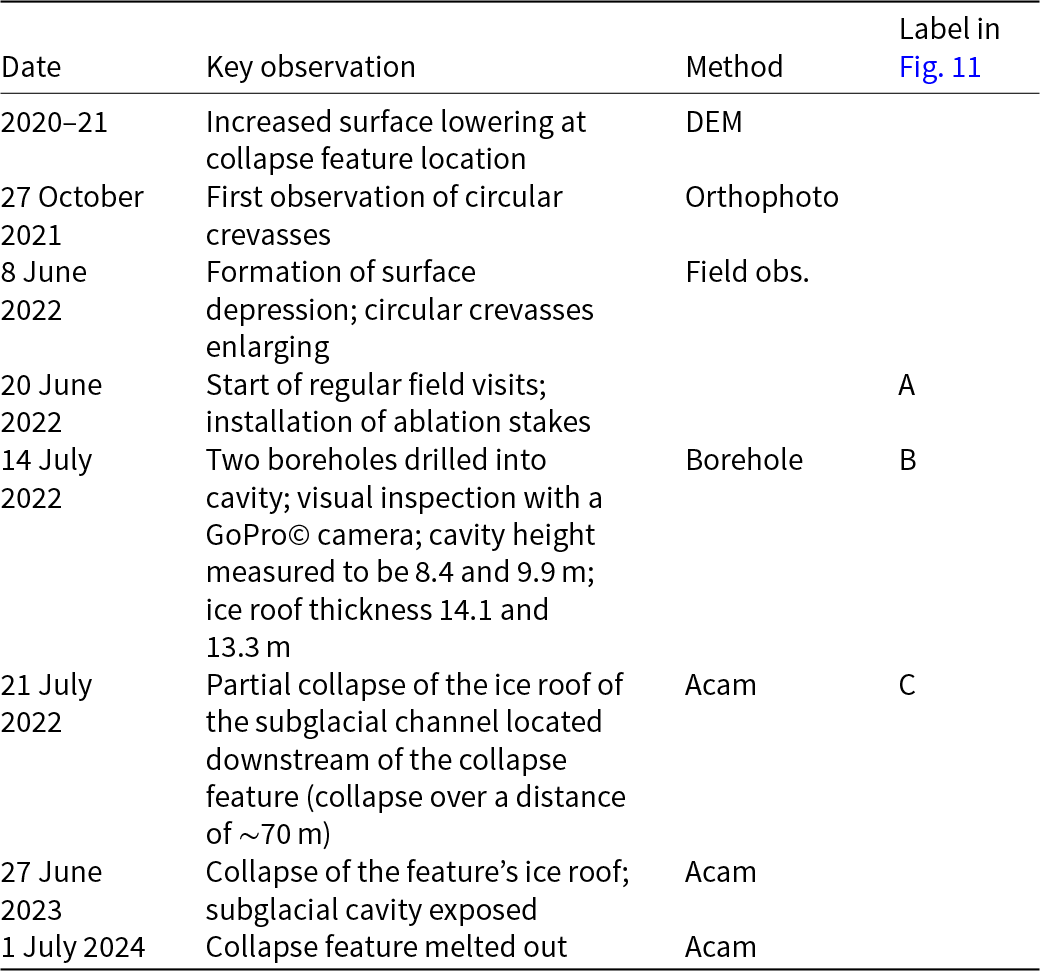
Abbreviations: ‘Field obs.’ = field observation; ‘Acam’ = automatic camera.


 Open access