Retirement tax shields: A cohort study of traditional and Roth accounts

Abstract

In this paper, we study the relative tax advantages of traditional and Roth retirement accounts in the United States by examining the retrospective tax benefits of each account type for the 2003 cohort of retirees. We use the actual history of marginal tax rates at the individual level to estimate that the average tax shields of traditional and Roth retirement accounts‒the excess value of retirement consumption financed by those accounts relative to brokerage accounts‒were 68 percent and 47 percent, respectively. Traditional accounts were better for this cohort largely due to tax cuts in 2001 and 2003. Under a counterfactual with inflation-adjusted 2019 law, the average tax shields for traditional and Roth accounts would have been much closer (33% and 30%, respectively), and nearly half of savers would have achieved higher retirement by saving in Roth accounts rather than in traditional accounts. This is the first paper to apply the history of marginal tax rates‒informed by administrative income records‒to compare Roth and traditional accounts for a particular cohort of retirees.

1. Introduction

Whether it is better for workers in the United States to save for retirement in a traditional account or a Roth account is a profoundly practical question. Many workers have both options through an employer’s defined contribution (DC) retirement plan, and many workers have access to both options as individual retirement arrangements (IRAs).

It is well known that Roth accounts tend to be favorable for a person who expects her marginal tax rate to be higher during retirement than during her working life, while saving in a traditional account tends to be favorable if the situation is reversed. Both account types shield investment returns from the tax that would otherwise apply to dividends, interest income, and capital gains‒that is, the ‘inside buildup’ is exempt from tax. Savings in Roth accounts are taxed as income before they are put into the account, and savings in traditional accounts are taxed as income when they are removed from the account. If investment returns are the same in both accounts and income tax is incurred exactly once for savings that passes through either account, then it should be better to pay income tax at whichever time the worker’s tax rate is lower.

However, predicting a marginal tax rate during retirement is not easy. Retirement income depends on years of savings decisions and investment returns, both of which are unknown ex ante. Furthermore, the schedule of marginal tax rates is a policy choice that changes over time and additionally interacts with the taxation of social security income in a complicated manner. Anticipating future marginal tax rates is somewhat difficult even for a worker close to retirement and extremely difficult for a worker far from retirement.

In this paper, we inform the traditional-or-Roth choice by examining the retrospective tax benefits of each account type for a particular cohort of retirees that retired in 2003. We use administrative tax records and a detailed tax calculator to construct tax rates in each year before and after retirement. We apply those tax rates and historical rates of return to estimate the present value of after-tax retirement income from traditional retirement accounts, Roth retirement accounts, and brokerage accounts with no tax benefits, all funded with equal contributions on an after-tax basis.

We consider two tax counterfactuals: one in which individuals faced the history of the tax system as it actually existed and one in which taxpayers faced the tax system as it existed in 2019 (adjusted only for inflation) throughout their entire lives. The former is most useful at answering a retroactive question: Would 2003 retirees have been better off by saving in a Roth or traditional account? The latter is most useful at answering a prospective question: Should current workers save in a Roth or traditional account?

We find that traditional accounts tended to dominate Roth accounts under the actual history of tax law faced by the cohort of 2003 retirees. On average, traditional accounts led to 68 percent more retirement wealth than if the equivalent after-tax savings were made in a taxable brokerage account, while Roth accounts lead to 47 percent more retirement wealth relative to taxable brokerage accounts; we refer to these quantities as the ‘tax shields’ of each type of account. This ranking was relatively stable across individuals: over 86 percent of individuals would have achieved more retirement wealth by saving in a traditional account instead of a Roth account. The dominance of traditional accounts is largely driven by the tax changes in 1986, 2001, and 2003, which meant that marginal tax rates tended to be higher in working age than in retirement.

By contrast, Roth and traditional accounts are much more comparable under the constant 2019 tax system. Traditional accounts and Roth accounts receive nearly the same tax advantage on average with a 33 percent average shield for traditional accounts and 30 percent for Roth accounts. The populations of savers are split nearly evenly between those who would have achieved higher wealth in a traditional account (53%) and those who would have achieved higher wealth in a Roth account (47%). This reflects the fact that we estimate marginal tax rates to be very similar in working age and in retirement under this counterfactual. Furthermore, the tax shield of both types of accounts is lower under the constant 2019 law counterfactual, relative to the actual history of tax law, as the 2019 tax system has tax rates on investment income that are generally lower than they were in the 1980s and 1990s.

We examine heterogeneity within the 2003 cohort. We find that, as predicted, workers whose replacement rates were higher‒that is, their retirement income was larger as a share of their working age income‒were relatively more likely to be better off using Roth accounts. Furthermore, holding working-age and retirement income fixed, having higher savings is associated with preferring Roth accounts. We find much more modest heterogeneity by gender and marital status.

We also consider the role of binding contribution limits. Because Roth accounts and traditional accounts have the same contribution limits but the former are made with after-tax dollars, savers can effectively shelter more savings under a Roth account. We find that, if individuals are consistently bound by contribution limits, most savers could achieve more wealth in a Roth account, even under contemporaneous law which favors traditional accounts in other circumstances. However, using an auxiliary dataset of working age individuals, we find that only about 14 percent of savers are constrained – thus, this additional consideration is not relevant for most individuals.

We are not the first to examine the relative benefits of traditional and Roth accounts. Crain and Austin (1997) were one of the first to study the relative benefits of traditional and Roth IRAs, finding that these benefits are closely tied to tax rates in working age and in retirement. A subsequent literature (discussed in detail in Adelman and Cross (2010)) considered variations of the Crain and Austin (1997) model and generally came to similar conclusions. Of note, Gokhale et al. 2001 argue that the complicated taxation of social security income has the effect of increasing marginal tax rates on other income types‒including IRA distributions‒in retirement, which is a factor favoring Roth accounts. Burman et al. (2001) argue that the post-tax nature of Roth accounts, in combination with flat dollar contribution limits, means that taxpayers can effectively save a larger amount in Roth accounts. Kotlikoff et al. (2008) find that the decision between Roth and traditional accounts is highly sensitive to assumptions regarding expectations about future tax changes.

More recently, Brown et al. (2017) examine traditional and Roth contributions as a portfolio choice question in the presence of uncertainty over future tax rates. They show that Roth accounts reduce the risk associated with uncertain future tax rates; this risk reduction favors Roth accounts relative to traditional accounts. Lachance (2013) uses a life cycle model to derive analytically optimal traditional-Roth portfolio allocation strategies in the presence of tax risk. In simulations using a dynamic life cycle model, Horneff et al. (2023) find that savings, investment, and consumption behavior under a traditional-only regime are very similar to behavior under a Roth-only regime.

Our paper differs from most of this literature in that we apply the actual history of earnings, family status, and other tax-relevant characteristics from administrative data – subject only to some linear interpolation between data years – rather than those simulated using dynamic programming tools. This provides a fuller, richer picture of marginal tax rates (including under various counterfactual tax regimes) throughout working age and retirement, which is necessary to compare Roth and traditional accounts both retrospectively and prospectively. Additionally, using the observed microdata allows us to study rich heterogeneity and answer questions about variance. For example, our data allow us to compute the share of individuals who achieve higher wealth with Roth accounts, even if traditional accounts achieve higher mean wealth.

The paper that is arguably closest to us is Marchand (2020), who studies the Canadian retirement system (which also has Roth-style and traditional-style accounts). Marchand (2020) uses a hybrid approach: simulating earnings paths not as the solution to a utility maximization problem, but solely to match observed moments in Canadian administrative data. We make several contributions relative to Marchand (2020). First, we study the United States instead of Canada; the United States tax system has unique features that affect retirement income and savings incentives, such as the complicated taxation of social security income and the saver’s credit. Second, we make several methodological refinements both in the accumulation and decumulation phases, which we discuss in the sections to follow.

Section 2 describes relevant features of the retirement system, Section 3 formalizes the basic mechanics of retirement accounts to facilitate comparisons across account types, Section 4 describes how we apply the principles of accumulation in retirement accounts to administrative data, and Section 5 presents the results. Finally, Section 6 concludes.

2. United States taxation of retirement savings

In general, savings in a taxable brokerage account generate investment earnings‒in the form of capital gains, interest income, and dividend income‒that is subject to taxation. To encourage retirement savings, the Internal Revenue Code allows investment earnings in a variety of retirement accounts to be exempt from such capital income taxation, that is, no tax is owed on interest, dividends, or capital gains that remain in the account. This treatment is sometimes referred to as ‘tax-free inside build-up’.

There are two classes of retirement accounts, which are distinguished by tax liability on contributions and distributions (also known as withdrawals). Contributions to a traditional account are made with pre-tax dollars‒that is, the labor income used to make such contributions is not taxed¹‒while distributions from a traditional account are generally taxed as ordinary income. Conversely, contributions to a Roth account are made with after-tax dollars and distributions from a Roth account during retirement are not taxed.²

Roth accounts and brokerage accounts have several characteristics in common. One characteristic shared by Roth accounts and brokerage accounts is that contributions are made with after-tax dollars. Another is that distributions are not subject to tax.³

The tax treatment of retirement plans and taxable brokerage accounts is summarized in Table 1. Relative to taxable accounts, both types of retirement accounts benefit from the exemption of capital income from taxation‒that is, the tax-free inside build-up. The distinction between Roth and traditional accounts is the timing of tax liability. Again, relative to taxable accounts, traditional contributions receive a subsidy that is offset by a tax cost for distributions. Roth accounts receive neither this subsidy nor this cost.

Table 1. Tax status of retirement account flows

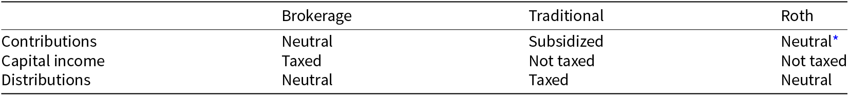
Notes: This table summarizes the tax treatment of retirement accounts and taxable brokerage accounts. See Section 2 for further details.

* Roth contributions are subsidized to the extent that they are eligible for the savers credit.

Since 2002, contributions to both Roth and traditional accounts have additionally been subsidized by the saver’s credit.⁴ The credit was equal to a percentage of the first $2,000 of contributions per person. This percentage was 50 percent, 20 percent, or 10 percent, depending on adjusted gross income (AGI). In 2019, the percentage was 50 percent for joint filers with AGI of $38,500 or less, 20 percent for joint filers with AGI between $38,501 and $41,500, and 10 percent for joint filers with AGI between $41,501 and $64,000. Joint filers with income above $64,000 were not eligible. Single filers faced the same ‘staircase’ schedule, except that all income amounts are cut in half. Critically, the credit is non-refundable. This means that taxpayers with income below the standard deduction, or with substantial other non-refundable credits (such as the child and dependent care credit) do not receive a benefit from the saver’s credit.

For tax years after 2026, the SECURE 2.0 Act of 2022 made several changes to the saver’s credit. First, it changed the mechanism from a tax credit claimed on Form 1040 to a match deposited directly into a traditional account of the saver’s choosing. Second, it made the credit refundable (i.e., the match is not limited by tax liability). Third, it replaced the staircase percentage schedule with a smooth phaseout (between $41,000 and $71,000 in income for joint filers).

Most retirement contributions are to plans sponsored by an employer. Employer plans are typically referred to by the section of the Code that enables them, for example, 401(k) or 403(b) plans; we refer to these plans in general as employer-sponsored DC plans, or just employer-sponsored plans for short. Workers are also permitted to obtain the same tax benefits by saving in IRAs that are not sponsored by an employer. However, not all individuals are allowed to benefit fully from IRAs: individuals with access to an employer-sponsored plan or a defined benefit plan (or whose spouse has such access) are not able to make traditional IRA contributions with pre-tax dollars, and there are income limits to making direct Roth IRA contributions.⁵ In general, there are no income limits to making contributions to employer-sponsored plans. IRAs came into existence in 1975, created by Congress in the Employee Retirement Income Security Act (ERISA). Employer-sponsored DC plans began in earnest shortly thereafter upon the passage of the Revenue Act of 1978.

Both employer-sponsored plans and IRAs are subject to annual limits on the amount that can be contributed, with the limit applying to the sum of contributions to Roth and traditional accounts. The annual limits for contributions to employer-sponsored plans are higher than the annual limits for contributions to IRAs. Contribution limits to employer-sponsored plans and to IRAs are higher for workers who are at least 50 years old than for workers under age 50. In 2019, the IRA annual limit was $6,000, or $7,000 if age 50 or older; the limit for employer-sponsored plans was $19,000, or $25,000 if age 50 or older. At some employers, non-discrimination rules cause the employer-sponsored plan limit to be effectively lower for certain highly compensated employees.

Importantly, IRAs often serve as a vehicle for collecting funds previously saved in a DC plan. Upon job separation, it is common (and in some cases, required by the former plan) for individuals to ‘roll over’ their DC balances into an IRA. So long as the DC plan and IRA are the same type (traditional or Roth), such rollovers have no tax consequences. Goodman et al. (2021) show that the vast majority of IRA assets reflect rollovers of previous DC contributions rather than contributions made directly to the IRA. Relatedly, they show that there are substantially more retirement-age distributions made from IRAs than from DC accounts, suggesting that most DC balances tend to be rolled over into IRAs before or shortly after the beginning of the decumulation phase.

Participation in DC plans and IRAs is widespread but far from universal. Hoffman et al. (2022) estimates that 18 percent of working-age individuals owned an IRA in 2020, while 35 percent owned a DC account. Participation differs by demographic characteristics; among working-age individuals, 54 percent of non-Hispanic white individuals owned either an IRA or DC account, while only 37 percent of non-Hispanic black individuals and 28 percent of Hispanic individuals did so. Additionally, Investment Company Institute (2024) showed that DC participation is increasing in income: those with household income over $100,000 participate at nearly three times the participation rate of those with household income under $50,000.

3. Conceptual approach

This section formalizes the basic mechanics of retirement accounts to facilitate comparisons across account types.

We start by characterizing how an account balance evolves from one year to the next in a brokerage account, a Roth account, or a traditional account. We then define the tax shield of Roth and traditional accounts relative to brokerage accounts and summarize how we apply these principles to data.

3.1. Brokerage accounts

The balance of a brokerage account with no tax benefits evolves according to the following law of motion for each individual i:

(1)\begin{equation} B^{BROK}_{i,t+1} = (1+r_{t}(1-\tau^K_{it})) \Big{(} B^{BROK}_{it} + S^{BROK}_{it} - D^{BROK}_{it} \Big{)} \end{equation}

where B is the balance in the account, S is after-tax contributions to the account (savings), D is after-tax distributions from the account (consumption), r is the rate of return, and τ ^K is the tax rate on capital income.⁶ The balance is constrained to be at least zero in all periods, that is, $B^{BROK}_t \geq 0$ for all t. For tractability, we assume that capital income is taxed on accrual. (In reality, dividends and interest are taxed on accrual, but capital gains are not.) In general, we expect S > 0 and D = 0 during the working life of the worker, and we expect S = 0 and D > 0 during retirement.

Let $\tilde{R}_i^{s,t}$ be the cumulative gross return from time s to time $t \geq s$, equal to $\Pi_{j=s}^{t-1} (1+r_{j}(1-\tau^K_{ij}))$.⁷ Using the law of motion, we can derive several useful expressions. First, a worker who started saving in a brokerage account at time $\underline{t} \lt t$ and has never taken a distribution from the brokerage account would have a balance given by the following equation:

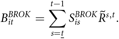(2)\begin{equation} B^{BROK}_{it} = \sum_{s=\underline{t}}^{t-1} S^{BROK}_{is} \tilde{R}^{s,t}. \end{equation}

In Section 4.2, we use a version of Equation (2) to guide our imputation of savings in a way that is consistent with the observed balance in the base year.

Second, for a worker who has balance $B^{BROK}_{it}$ at time t, does not make any contributions at time t or later, and lives until time $\overline{t} \geq t$, the budget constraint requires:

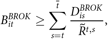(3)\begin{equation} B^{BROK}_{it} \geq \sum_{s=t}^{\overline{t}} \frac{D^{BROK}_{is}}{\tilde{R}^{t,s}} \text{,} \end{equation}

which we will assume holds with equality in our empirical applications.

3.2. Roth accounts

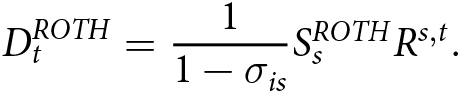
The balance of a Roth account evolves according to the following law of motion:

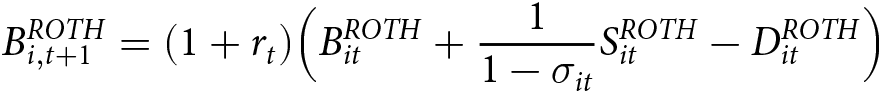(4)\begin{equation} B^{ROTH}_{i,t+1} = (1+r_{t}) \Big{(} B^{ROTH}_{it} + \frac{1}{1-\sigma_{it}} S^{ROTH}_{it} - D^{ROTH}_{it} \Big{)} \end{equation}

where B is the balance in the account, S is after-tax contributions to the account (savings), D is after-tax distributions from the account (consumption), r is the rate of return, and σ is the subsidy due to the saver’s credit. The subsidy due to the saver’s credit has an individual subscript because it depends on the individual worker’s income and retirement contributions. As expressed in this equation, σ is the saver’s credit percentage per dollar of retirement contributions.

Let $R^{s,t}$ be the cumulative pre-tax gross return from time s to time $t \geq s$, equal to $\Pi_{j=s}^{t-1} (1+r_{j})$.⁸ Relative to a brokerage account, a Roth account benefits from (1) the absence of tax on capital income (τ_k) and (2) the presence of a subsidy on savings (σ). These benefits are visible by comparing the law of motion for brokerage accounts (Equation (1)) to the law of motion for Roth accounts (Equation (4)). The balance in a Roth account for a worker who started saving at time $\underline{t} \lt t$ and has never taken a distribution is given by:

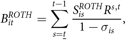(5)\begin{equation} B^{ROTH}_{it} = \sum_{s=\underline{t}}^{t-1} \frac{S^{ROTH}_{is}R^{s,t}}{1-\sigma_{is}} \text{,} \end{equation}

where the absence of tax on capital income is expressed here by using R rather than $\tilde{R}$.

Distributions for a worker who makes no contributions at time t or later and lives until time $\overline{t}$ are constrained by the balance in year t:

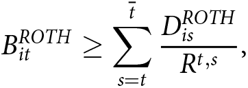(6)\begin{equation} B^{ROTH}_{it} \geq \sum_{s=t}^{\overline{t}} \frac{D^{ROTH}_{is}}{R^{t,s}} \text{,} \end{equation}

which we will assume holds with equality in our empirical applications.

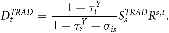
3.3. Traditional accounts

The balance of a traditional account evolves according to the following law of motion:

(7)\begin{equation} B^{TRAD}_{i,t+1} = (1+r_{t}) \Big( B^{TRAD}_{it} + \frac{1}{1-\tau^Y_{it}-\sigma_{it}} S^{TRAD}_{it} - \frac{1}{1-\tau^Y_{it}} D^{TRAD}_{it} \Big) \end{equation}

where B is the balance in the account, S is after-tax contributions to the account (savings), D is after-tax distributions from the account (consumption), r is the rate of return, σ is the subsidy due to the saver’s credit, and τ ^Y is the tax rate on ordinary income. The two expressions with the tax rate on ordinary income adjust for the facts that (1) income that is contributed to a traditional account is exempt from income tax and (2) distributions from traditional accounts are taxed as income.

The balance in a traditional account for a worker who started saving at time $\underline{t} \lt t$ and has never taken a distribution is given by:

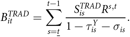(8)\begin{equation} B^{TRAD}_{it} = \sum_{s=\underline{t}}^{t-1} \frac{S^{TRAD}_{is}R^{s,t}}{1-\tau_{is}^Y-\sigma_{is}}. \end{equation}

Distributions for a worker who makes no contributions after time t and lives until time $\overline{t}$ are constrained by the balance in year t:

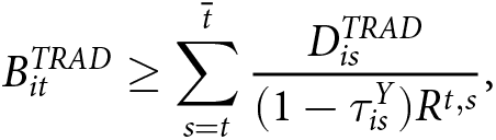(9)\begin{equation} B^{TRAD}_{it} \geq \sum_{s=t}^{\overline{t}} \frac{D^{TRAD}_{is}}{(1-\tau_{is}^Y)R^{t,s}} \text{,} \end{equation}

which we will assume holds with equality in our empirical applications.

3.4. Account type comparisons

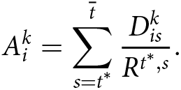
We compare the present value of retirement consumption in each account type from the perspective of the time of retirement $t^*$, which we define as the period after the final period in which savings are contributed to the account. For a worker who makes no contributions in time $t^*$ or later and lives until time $\overline{t}$, the present value at time $t^*$ of retirement consumption financed by an account of type $k \in$ (brokerage, traditional, Roth) is given by the following equation:

(10)\begin{equation} A_{i}^{k} = \sum_{s=t^*}^{\overline{t}} \frac{D_{is}^{k}} {R^{t^*,s}}. \end{equation}

In this expression, A is the present value of retirement consumption at the time of retirement, D is the current value of net-of-tax financed retirement consumption in some future period, and R is the gross discount rate, which we assume is the same as the cumulative pre-tax gross return. This same equation is used for the present value of retirement consumption financed by brokerage, Roth, and traditional accounts.

The expression of present value (A) in Equation (10) can be compared across account types. Balances in a particular year (B) are not comparable because (1) accumulation inside a brokerage account differs from accumulation inside Roth and traditional accounts and (2) distributions from traditional accounts are taxed but distributions from brokerage and Roth accounts are not. The present value of retirement consumption financed by an account is an apples-to-apples measure that can be compared across brokerage, Roth, and traditional accounts.

Note that the present value of retirement consumption is equal to the balance in the year of retirement for Roth accounts ( $A^{ROTH}_i=B^{ROTH}_{i,t^*}$) and less than the balance in the year of retirement for traditional accounts ( $A^{TRAD}_i \lt B^{TRAD}_{i,t^*}$) and brokerage accounts ( $A^{BROK}_i \lt B^{BROK}_{i,t^*}$). This can be seen by comparing Equation (10) with Equations (3), (6), and (9).

Standard comparison between Roth and traditional accounts

It is well known that traditional accounts are generally advantageous relative to Roth accounts if the working-age tax rate is higher than the retirement-age tax rate. This is easy to see in our model by deriving the distribution in a particular year of retirement that is attributable to savings from a particular year for Roth and traditional accounts.

If contributions are only made in a single year $s \lt t^*$ and distributions are only made in a single year $t \geq t^*$, then we can derive the following from the Roth law of motion (Equation (4)):

(11)\begin{equation} D^{ROTH}_{t} = \frac{1}{1-\sigma_{is}} S^{ROTH}_s R^{s,t}. \end{equation}

If contributions are only made in a single year $s \lt t^*$ and distributions are only made in a single year $t \geq t^*$, then we can derive the following from the traditional law of motion (Equation (7)):

(12)\begin{equation} D^{TRAD}_{t} = \frac{1-\tau^Y_{t}}{1-\tau^Y_s-\sigma_{is}} S^{TRAD}_s R^{s,t}. \end{equation}

Holding fixed after-tax savings ( $S^{TRAD}_s=S^{ROTH}_s$), and assuming for simplicity that the saver’s credit is zero ( $\sigma_{is}=0$), we can see from Equations (11) and (12) that retirement consumption financed by a traditional account exceeds retirement consumption by a Roth account ( $D^{TRAD}_{t} \gt D^{ROTH}_{t}$) if and only if the working-age tax rate exceeds the retirement-age tax rate ( $\tau^Y_{s} \gt \tau^Y_{t}$).⁹

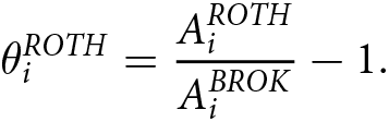
3.5. Tax shield

We define the tax shield of a retirement account as the excess present value of retirement consumption financed by the retirement account, measured as of the date of retirement $t^*$, over the present value of retirement consumption financed by a brokerage account with no tax benefits, holding fixed the path of after-tax savings. The tax shield of a Roth account is given by the following equation:

(13)\begin{equation} \theta_i^{ROTH} = \frac{A^{ROTH}_{i}}{A^{BROK}_{i}} - 1. \end{equation}

The tax shield of a traditional account is defined analogously:

(14)\begin{equation} \theta_i^{TRAD} = \frac{A^{TRAD}_{i}}{A^{BROK}_{i}} - 1. \end{equation}

We are interested in estimating and comparing $\theta^{ROTH}_i$ and $\theta^{TRAD}_i$.

4. Empirical strategy

This section describes how we use administrative tax records from 1969 through 2022 and other data sources to simulate the present value of retirement consumption in the year of retirement under various counterfactuals. We focus on the cohort that retired in 2003, meaning they contributed savings to a retirement account in 2002 and in no subsequent year. (That is, in the notation of Section 3.5, $t^* = 2003$.)

4.1. Overview

For each retiree in the cohort, we use the observed IRA balance in the year of retirement, in combination with an assumption on the profile of savings over the life cycle, to impute a path of after-tax savings S over the working life of the retiree. We use the logic of Equation (7) to ensure that the imputed path of after-tax savings is consistent with historical rates of return r, historical individual-level marginal tax rates $\tau_i^Y$, and the observed IRA balance in the year of retirement.

We then construct counterfactual balances in the year of retirement for each retiree. Using the logic of Equations (1), (4), and (7), the imputed path of after-tax savings S, historical rates of return r, and historical or simulated capital income tax rates $\tau^K_i$, we calculate a counterfactual balance in each type of account in the year of retirement.

Finally, for each account type, we assume that distributions for each individual match that individual’s observed distributions, multiplied by a person-specific factor to force the budget constraint to hold with equality. We then use the calculated path of distributions and historical rates of return r to calculate the present value of retirement wealth for each account type as given by Equation (10). Finally, we calculate the tax shield of Roth and traditional accounts as defined in Equations (13) and (14).

In our baseline analysis, we consider three counterfactual saving vehicles: traditional plans, Roth plans, and taxable brokerage accounts. We interact these saving vehicle counterfactuals with two assumed legal systems: one in which individuals faced the tax system as it existed in 2019 (adjusted for inflation) throughout their entire lives and one in which individuals faced the history of the tax system as it actually existed. Across all counterfactuals, we hold fixed the amount of saving, denoted S_it.

Broadly speaking, the empirical procedure has two main parts:

1. (1) First, we identify a cohort of interest and construct a long panel from 1960 through 2022 for each individual in the cohort.

2. (2) Second, we use the panel to compute retirement wealth under various counterfactuals.

We discuss each in turn.

4.2. Constructing the panel

Sample

We define a fixed cohort of approximately 800,000 workers that we deem to have retired in 2003. The workers in this cohort: (1) were age 55–70 in 2003, (2) contributed to a workplace DC account or made a non-rollover contribution to a traditional or Roth IRA in 2002, (3) did not make a non-rollover contribution to either type of account in any subsequent year, (4) had a balance in a traditional or Roth IRA entering 2003 or subsequently engaged in a rollover to an IRA at some future point, and (5) made a distribution from a traditional IRA at any point in 2003 or later. We require that individuals were alive through the end of 2005. For computational tractability, we use a 10 percent random sample of this cohort in all of our analyses.

Whether a worker contributed to a retirement account in a particular year is coded based on Form W-2, Box 12 (Codes D, E, F, G, H, S for elective deferrals) and Form 5498, Box 1 (Contributions) for that tax year. Whether an individual had a balance in a traditional IRA is based on Form 5498, Box 5 (Fair Market Value) and Box 7 (IRA checkbox); rollovers are determined from Form 5498, Box 2 (Rollover contributions). Age is calculated from a database of birth dates for all individuals who have ever been issued a Social Security Number or Individual Tax Identification Number.

We focus on individuals who retired in 2003 to give us the longest possible series of retirement tax rates for a clean cohort of retirees. The electronic records we use do not contain information on DC contributions in 2001 (or any year before 1999), so for years earlier than 2002 our method of defining a retiring cohort‒looking at the final year in which contributions to a retirement plan were made‒would be inaccurate.

The restriction to IRAs reflects a limitation of our data. Ideally, we would include all individuals with an IRA balance or a balance in an employer-sponsored DC plan; unfortunately, the tax data contain information on only the former (on Form 5498), not the latter. However, Goodman et al. (2021) show that it is a reasonable approximation that most assets saved in employer-sponsored accounts are rolled over into an IRA before the bulk of retirement-age distributions begin. Thus, we interpret our restriction to holding an IRA entering 2003, or rolling assets into an IRA at some later point, as capturing a large share of wealth initially saved in employer-sponsored accounts rather than IRAs themselves. We compute an individual’s ‘observed’ IRA balance entering 2003 as equal to the IRA value entering 2003 plus the present value of subsequent rollovers (discounted using the rates of returns as discussed below under the heading ‘Rates of return and portfolio composition’).

Table 2 shows that the median worker in the sample had a traditional IRA balance entering 2003 of $49,000. The median worker had earned average working-age wages of $31,000 (in 2003 dollars). In 2003, the average age of workers in the sample was 62, and 75 percent of workers in the sample were married. As of late 2024, 61 percent of workers in the sample were still alive.

Table 2. Summary statistics of analysis cohort

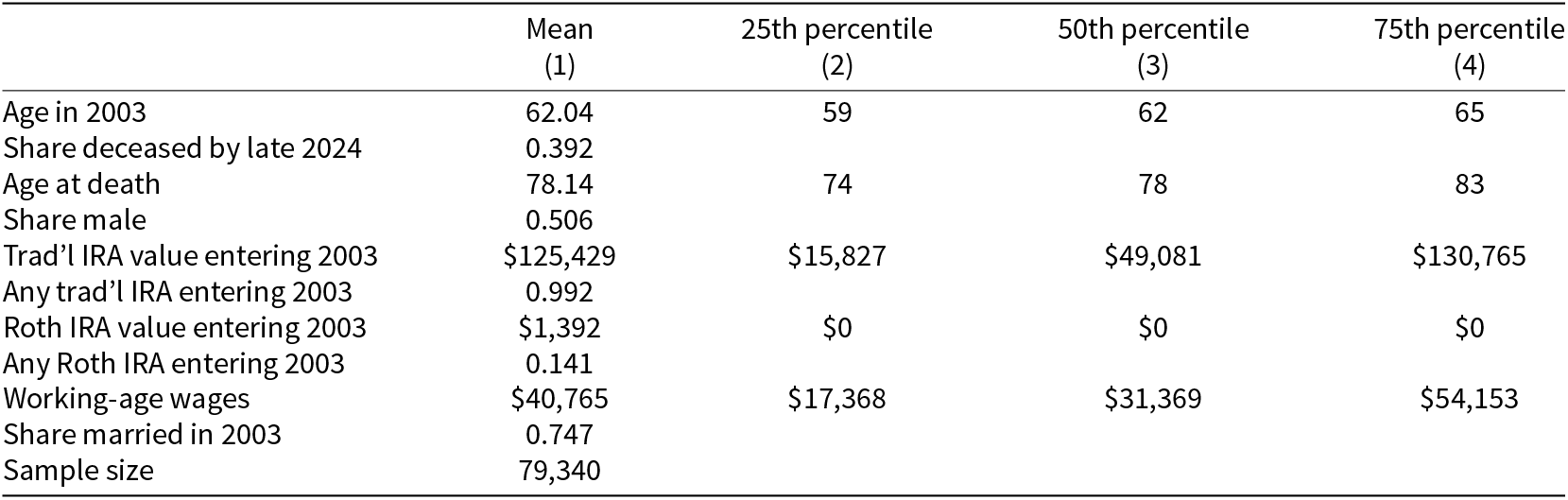
Notes: This table reports summary statistics for the sample used in our analysis. All percentiles are pseudo-percentiles, equal to the mean of the 10 observations closest to the true quantile. Working-age wages are expressed in 2003 dollars.

Creating the panel from 1999 onward

From 1999 onward, our database contains the universe of Form 1040 tax returns as well as information returns such as Forms W-2, 5498, 1099-R (for retirement distributions), and 1099-SSA (for social security benefits). In particular, from Form 1099-R, we can identify distributions from a given individual’s IRA. We are also able to directly observe wages from Form W-2 over this time period. We observe an individual’s state of residence from their Form 1040.¹⁰

Creating the panel prior to 1999

Our data are more incomplete prior to 1999. From 1996 to 1998, we observe the usual set of variables from Form 1040 and its schedules, but not from any information returns. Prior to 1996, we have access to the population of Forms 1040 in roughly five-year intervals‒specifically, 1969, 1974, 1979, 1984, 1989, 1994, and 1995. However, these years are ‘narrower’ datasets, meaning that we do not observe as much detail about income sources or deductions. Therefore, we must make various imputations, discussed in Appendix Section A.2. Finally, we linearly interpolate between years with data and extrapolate backward from 1969 to 1960, as also discussed in Appendix Section A.2.

Rates of return and portfolio composition.

We construct annual rates of return from yields on 10-year Treasury bonds and a broad index of domestic stock market returns based on Fama and French (1993).¹¹ We give a 40 percent weight to Treasury yields and a 60 percent weight to stock market returns.

Imputing savings

We impute contributions during working age as follows, each designed to mimic the observed IRA balance in 2003.¹² In particular, we consider several particular profiles of (net-of-tax) saving as a share of (net-of-tax) wages. This leads to savings equations that have the form $S_{it} = \alpha_i \times f_{it} w_{it}$, where f_it is some deterministic path, w_it is net-of-tax wages, and α_i is a scaling factor that (in combination with assumed rates of return) is pinned down by the actual IRA balance entering 2003. We abstract from any contribution limits, though we consider them in Section 5.3.

The simplest version of f_it is a constant‒reflecting an assumption that individuals save a constant share of their wages. However, this conflicts with empirical evidence that the savings rate tends to increase as one approaches retirement (Parker et al., 2022). In our baseline method, we estimate $f_{it} = g(age_{it})$ directly from an auxiliary sample of individuals in the tax data. In particular, we take a 1 percent sample of individuals who save a positive amount at any point from 2002 to 2006.¹³ Among this sample, we estimate the average retirement savings rate in 2004‒that is, the net-of-tax retirement savings as a share of net-of-tax wages‒by single year of age. We set $g(age_{it})$ equal to these means. Appendix Figure B.1 shows that savings rates increase fairly linearly, crossing 2 percent around age 24 and 8 percent around age 58. This is broadly consistent with the patterns found in Parker et al. 2022.¹⁴

One complication to this imputation is that IRAs did not exist until 1975. We proceed by assuming that savings S_it from 1960 and 1974 were contributed to a taxable account.¹⁵ Then, we assume that the net-of-tax wealth located in the taxable account is transferred gradually, between 1975 and 1980, to a traditional account. Additional details and implications of this assumption are provided in Appendix A.3.

In sum, these assumptions are sufficient to allow us to estimate α_i and thus the path of S_it. This path is then held constant across all simulations.¹⁶

4.3. Estimating counterfactual retirement wealth

In this subsection, we discuss how we use the inputs constructed in Section 4.2 to estimate $A_i^{TRAD}$, $A_i^{ROTH}$, and $A_i^{BROK}$. That is, holding net-of-tax saving fixed, what is the net-of-tax wealth held by individuals under the counterfactual where all of their saving is in traditional accounts, Roth accounts, or taxable accounts? Broadly speaking, our task is to estimate each element in Equations (8), (9), and (10) and their analogues for Roth and taxable accounts. We do so under two legal counterfactuals: one in which individuals faced the contemporaneous tax system as it actually existed in each year, and another in which individuals faced the 2019 tax system in all years (with all statutory parameters adjusted for inflation). For the former, we take into account that IRAs and similar accounts did not exist prior to 1975; for the latter, we assume access to such accounts throughout working life.

The accumulation phase.

The primary objects to compute are the tax rates ( $\tau_{it}^Y$) and saver’s credit rates (σ_it).¹⁷ To do so, We make use of NBER TAXSIM (Feenberg and Coutts, 1993), augmented by us to calculate the saver’s credit. NBER TAXSIM is a detailed tax calculator that captures most of the important features of federal and state income taxes; thus, $\tau_{it}^Y$ reflects the marginal rate schedule but also reflects the phase-in and phase-out of credits such as the earned income credit, the interaction with the taxation of social security income, and the (full or partial) deductibility of state income taxes. Our ability to closely approximate the actual history of tax rates at the individual level distinguishes this paper from others that compare Roth and traditional retirement accounts.¹⁸

Additionally, we approximate the annual rate of return in taxable accounts, $\widetilde{r}_{it} = r_t(1-\tau^K_{it})$. To do so, we compute marginal tax rates on qualified dividends, taxable interest, and long-term capital gains which vary by individual. We assume that 50 percent of the return is taxed as long-term capital gains, 25 percent as qualified dividends, and 25 percent as taxable interest. We assume that the accrual-equivalent capital gains rate is two thirds of the statutory rate; this would be consistent with a 15-year holding period and 7.5 percent pre-tax rate of return. We can then compute the tax rate that applies to each component of the investment return, and we set $\tau^K_{it}$ equal to the weighted average.

The decumulation phase

The remaining objects to compute are the balances at retirement, $B_{i,2003}$ and the path of net-of-tax distributions (D_it). The balances are computed using Equation (2) and their Roth and traditional analogues. To simulate the path of distributions, we assume that pre-tax distributions (denoted $d_{it}^k$) from account type $k \in$ (traditional, Roth, brokerage) are proportional to observed distributions from traditional accounts, that is, we assume

(15)\begin{equation} d_{it}^k = \theta_i^k \times d_{it,obs}^{TRAD}\text{,} \end{equation}

where $d_{it,obs}^{TRAD}$ is observed distributions from traditional IRAs from person i in year t. We solve for $\theta_i^k$ for each individual by imposing the budget constraint (i.e., Equation (3) and its analogues). This approach contrasts to that of Marchand (2020), who compute the retirement marginal tax rate with respect to a small change in income at a single point in time (age 70). Our approach meaningfully refines Marchand (2020) to reflect the actual timing of distributions during retirement; furthermore, our approach picks up the effect of lumpy distributions being associated with an atypically high average tax rate, while Marchand (2020) abstracts from that effect.

Given the path of pre-tax distributions in the traditional counterfactual, $d_{it}^{TRAD}$, we can then compute $\tau_{it}^Y$, the average tax rate that applies to that distribution. We again use NBER TAXSIM, which we stress correctly takes into account the partial taxation of social security income, which is critical for this population (Gokhale et al., 2001).

The pre-tax distributions and the average tax rate that apply to them are sufficient to recover the net-of-tax distributions, D_it. Given the path of distributions and rates of returns calculated earlier, we can then compute $A_i^{TRAD}$, $A_i^{ROTH}$, and $A_i^{BROK}$ using Equation (10).

5. Results

Table 3 summarizes the benefits of Roth and traditional retirement accounts for the cohort of workers that retired in 2003. We estimate (column 1) the average tax shield of traditional retirement accounts for the 2003 cohort was 0.68 under contemporaneous law; that is, an average worker who retired in 2003 would have financed an additional 68 percent of retirement consumption by saving in a traditional retirement account instead of a taxable brokerage account. We estimate that the average tax shield of Roth accounts for the 2003 cohort was 0.47. Thus, for the 2003 cohort on average, we find that traditional accounts offered a larger tax shield than Roth accounts. Equivalently, saving in traditional accounts would have financed more retirement consumption on average than saving in Roth accounts for the 2003 cohort.

Table 3. Main results: Average tax shield of Roth and traditional accounts relative to taxable accounts

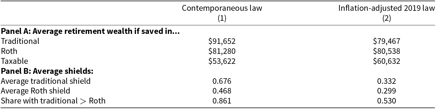
Notes: Panel A presents the average present value of retirement consumption financed through traditional, Roth, and taxable accounts. Panel B presents the average (person-weighted) tax shield of traditional and Roth accounts and the share of individuals for whom traditional accounts would have financed more retirement consumption than Roth accounts. Note that the quantities in Panel B cannot be derived directly from the quantities in Panel A; due to implicit differences in weighting, the average shield is not equal to the shield implied by the average values of wealth.

Traditional accounts outperforming Roth accounts for the 2003 cohort is partially explained by changes in Federal tax policy. As noted earlier, traditional accounts tend to be better if the tax rate faced by an individual is lower during retirement than during the individual’s working life. Legislation in 1986, 2001, and 2003 reduced marginal tax rates generally, so the cohort of workers that retired in 2003 tended to face a lower tax rate schedule during retirement than during their working lives. Under contemporaneous law, we estimate that the vast majority of the cohort‒85 percent‒would have financed more retirement consumption by saving in traditional accounts than in Roth accounts.

Using the same individual earnings and savings history but under the counterfactual of constant inflation-adjusted 2019 tax law, we find that Roth and traditional accounts offered nearly the same shield on average. Table 3 shows that, in the 2019-law counterfactual, we estimate an average tax shield of traditional accounts of 0.33 and an average tax shield of Roth accounts of 0.30. We estimate a roughly even number of savers would prefer each type of account – 53 percent of the cohort would have financed more retirement consumption by saving in traditional accounts than by saving in Roth accounts.¹⁹

5.1. Determinants of tax shields

Table 4 summarizes key determinants of retirement account tax shields. For traditional accounts, the difference in marginal tax rates between working age and retirement is very important. Under contemporaneous law (Panel A), we find that average marginal tax rates during working age were 31.1 percent, meaning that traditional contributions received a subsidy at a 31.1 percent rate. At retirement, traditional distributions are taxed as ordinary income, while Roth distributions are not taxed. We find that traditional distributions would have faced an average marginal tax rate of 22.2 percent under contemporaneous law.²⁰ This 9 percentage point wedge causes traditional accounts to tend to dominate Roth accounts under contemporaneous law. The saver’s credit is negligible in this legal counterfactual because the saver’s credit was in effect for only one year of working life of this cohort.

Table 4. Key ingredients in calculation of tax shields

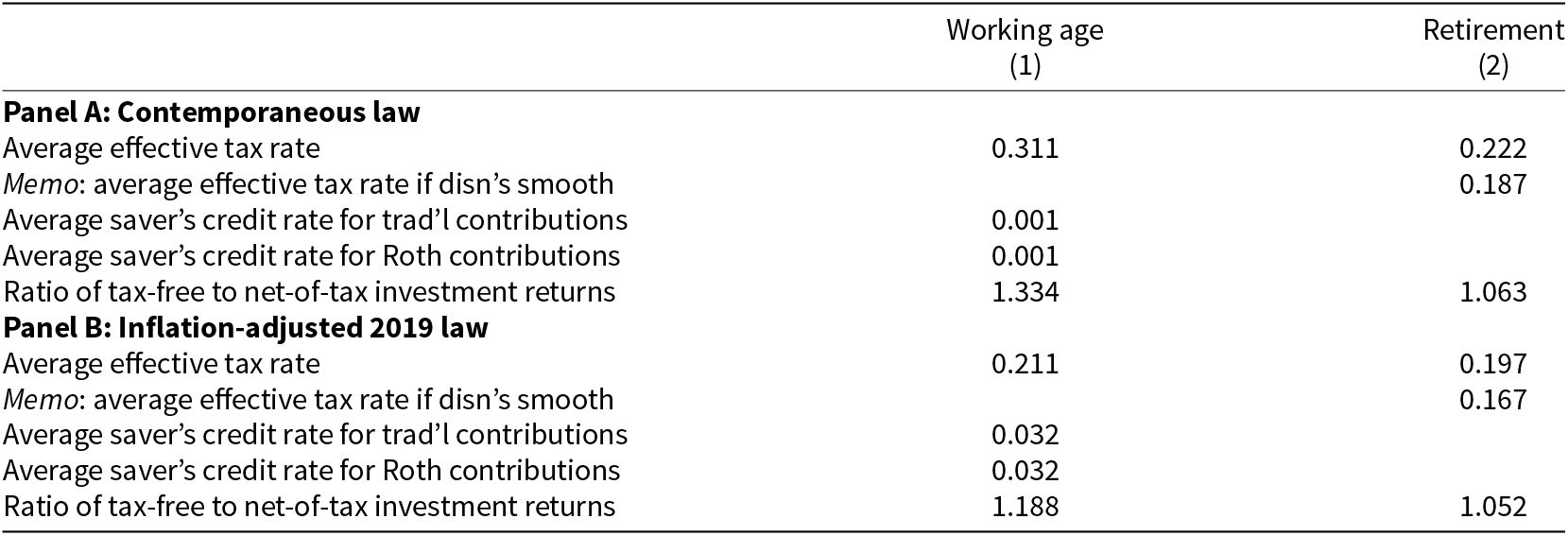
Notes: This table reports several of the main inputs that determine the tax shields of Roth and traditional retirement accounts. The average effective tax rate is the marginal income tax rate on one dollar of wage income (during working age) or on one dollar of taxable IRA distributions (during retirement), including federal and state income taxes and their interaction. The saver’s credit rates are equal to the total saver’s credit (after the tax liability limitation) divided by the amount of the contribution. The effective tax rates and saver’s credit rates are collapsed to the individual level, weighting by the present value of traditional contributions. In working age, tax-free and net-of-tax gross investment returns are collapsed to the individual level weighted by nominal traditional contributions. In retirement, the ratio of tax-free to net-of-tax gross investment returns is calculated as the ratio of the brokerage balance at retirement $B_{it^*}^{BROK}$ to its present value $A_{i}^{BROK}$ as defined by Equation (10). The numbers in this table are an unweighted average across individuals.

Under inflation-adjusted 2019 law (Panel B), the wedge between the working-age subsidy and the retirement-age tax rate was much smaller. Traditional contributions received a subsidy of 21.1 percent from the regular tax schedule and an additional 3.2 percent from the saver’s credit under inflation-adjusted 2019 law. Roth contributions received a subsidy of 3.2 percent from the saver’s credit. Traditional distributions would have faced an average marginal tax rate of 19.7 percent under inflation-adjusted 2019 law. Because this wedge is much smaller than under contemporaneous law, the advantage to traditional accounts is also much smaller.

One force pushing the effective tax rate higher in retirement is that individuals tend not to time their distributions in a tax-efficient way. To quantify this, we compute the effective tax rate under an alternative assumption that distributions are made smoothly over the entire retirement period.²¹ Under inflation-adjusted 2019 law, the effective tax rate in retirement would be about 3 percentage points lower (16.7%), as indicated in the ‘memo’ line in Table 4 – a meaningful amount relative to the overall wedge between working age and retirement effective tax rates.

This gap between true distributions and hypothetical smoother distributions occurs for two reasons. First, true distributions are lumpy – that is, the effective tax rate in a given year is made higher by the IRA distribution itself. Second, it turns out that retirees tend to take distributions exactly when their tax rate would otherwise be higher, IRA distributions aside. To decompose the relative role of these two effects, we compute a ‘hypothetical’ average effective tax rate where the effective tax rate in each year is given under the smooth distribution counterfactual (so that the effect of the IRA distributions themselves on tax rates is eliminated), but we weight across years using the true path. We calculate this hypothetical tax rate, averaged across individuals, to be 18.4 percent. The gap between 19.7 percent and 18.4 percent – about 44 percent of the wedge – represents the direct effect of lumpy distributions, while the gap between 18.4 percent and 16.7 percent represents the effect of the correlation between IRA distributions and IRA-exclusive tax rates.²²

We stress that the measured tax rates in retirement (and in working age, to the extent that it applies) correctly take into account the partial taxation of social security income. In particular, the amount of social security income that is subject to tax is a function of the amount of non-social security income. As noted by Gokhale et al. 2001, this can have the effect of increasing the marginal tax rate on other income by 50 or 85 percent for those affected. NBER TAXSIM incorporates this calculation. We estimate that, on average, the marginal tax rate would be 2.4 (contemporaneous law) or 2.1 (inflation-adjusted 2019 law) percentage points lower if the distribution did not increase the amount of social security income subject to federal income tax. In sum, our results are consistent with Gokhale et al. 2001 in that taxation of social security income does increase retirement-age tax rates, but we find that this effect is smaller on average than the reduction in marginal tax rates due to the general reduction in income that tends to occur at retirement.

Next, we turn our attention to the role of the saver’s credit. The average saver’s credit rate is noteworthy for several reasons. First, the fact that the saver’s credit rate is virtually identical between traditional and Roth contributions means that, for the vast majority of individuals who have household income such that they can benefit from the saver’s credit ($32,000 for single filers and $64,000 for joint filers), retirement contributions are under $2,000 per year in 2019 dollars.²³ Second, given the nearly identical average saver’s credit rate, the saver’s credit effectively subsidizes traditional contributions by more than Roth contributions, since each dollar of traditional contributions requires less after-tax saving yet yields the same saver’s credit. Third, the fact that the average saver’s credit rate is substantially less than the statutory rates of 50 percent, 20 percent, and 10 percent implies that most savers have income that it is too high or tax liability too low to benefit from the saver’s credit, reducing the overall subsidy‒and slight advantage to traditional accounts‒created by the saver’s credit.²⁴

Figure 1 provides more detail on the time path of marginal tax rates. It shows that, under contemporaneous law, marginal tax rates were substantially higher through the mid-1980s than they were in the 2000s. The Tax Reform Act of 1986 reduced marginal rates somewhat, but they remained higher than 2019 law until the passage of the Tax Cuts and Jobs Act of 2017. Meanwhile, Figure 1 also shows that marginal tax rates would have increased gradually under inflation-adjusted 2019 law over the working lives of the cohort, then dropped sharply at retirement. Under a stable tax law regime with graduated marginal tax rates, changes in marginal tax rates are primarily a consequence of changes in income. Income was higher during the working lives of the cohort than during retirement, so marginal tax rates were also higher.²⁵

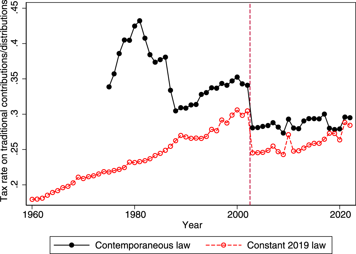
Figure 1. Average tax rates by year.

Note: This figure plots the average marginal tax rate by year in our cohort, including federal and state income taxes.

While the tax rates on contributions and distributions are the key factors determining the relative ranking between Roth and traditional accounts, the advantage of both types of retirement accounts over taxable brokerage accounts is largely driven by the benefit of tax-free inside build-up. In the fourth row of each panel of Table 4, we report the ratio of gross returns in retirement accounts to net-of-tax returns in taxable brokerage accounts. The tax-free inside build-up increases retirement wealth by 33 percent during working age and an additional 6 percent during retirement under contemporaneous law. The value of tax-free inside build-up is smaller under the inflation-adjusted 2019 law counterfactual: 19 percent during working age and an additional 5 percent in retirement. The difference between legal environments largely reflects tax changes in 2001 and 2003 that reduced the tax rates on dividends and capital gains held in taxable brokerage accounts, especially for low and moderate earners. For example, under 2019 law, joint filers with taxable income under $78,750 do not pay tax on long-term capital gains or qualified dividends, even in taxable accounts.

In Appendix B.2, we consider the robustness of our findings to varying the assumptions with respect to contribution timing, distribution timing, and portfolio composition. In brief, we find that assuming contributions later in working age relative to baseline and (as discussed above) assuming a smooth path of distributions tends to favor traditional accounts. Changing portfolio composition mechanically has no effect on the difference between Roth and traditional accounts (as we assume that the portfolio composition affects only the taxation of investment returns in a taxable account, not pre-tax returns); we find that the overall shield of retirement accounts roughly doubles relative to baseline if we assume portfolios consist entirely of taxable bonds. Interested readers are directed to Appendix B.2 for a more detailed discussion.

5.2. Heterogeneity

One of the advantages of our data is that we can look beyond mean shields; in particular, we can compute the shield for each individual for each type of account. This allows us to describe the distribution of the relative tax advantages of Roth and traditional accounts.

In Figure 2, we plot the density of the difference between the traditional tax shield and the retirement tax shield under each of the two legal counterfactuals; those to the right of zero achieve more wealth by saving in traditional accounts, while those to the left of zero achieve more wealth by saving in Roth accounts. The distribution peaks at about 0.1 under contemporaneous law and just to the left of zero (i.e., indifference) under inflation-adjusted 2019 law, but there is meaningful dispersion in both cases. Under contemporaneous law, the range from the 10th to 90th percentile is $[-0.022,0.496]$, while it is $[-0.117,0.234]$ under inflation-adjusted 2019 law.²⁶

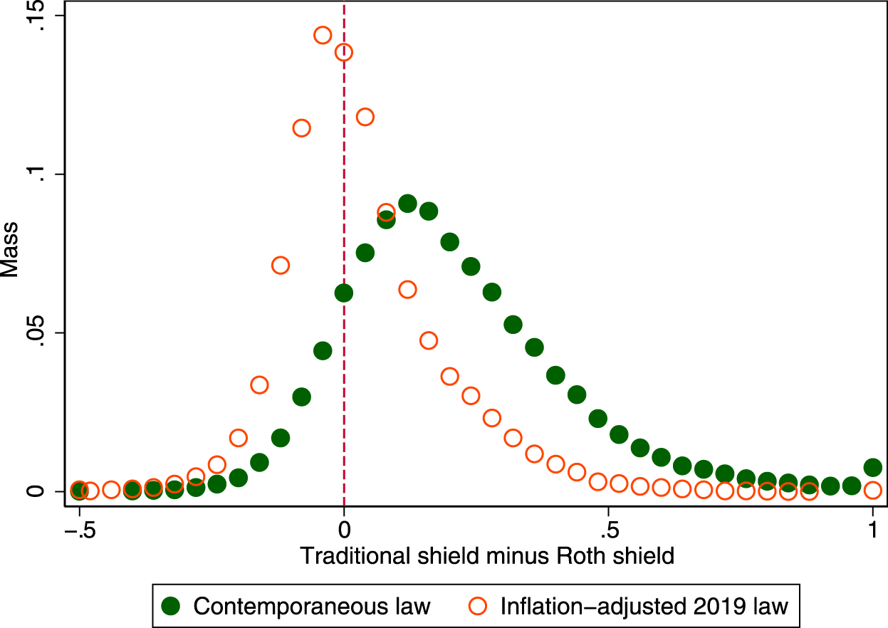
Figure 2. Histogram of the traditional shield minus the Roth shield.

Notes: This figure plots the probability mass function of the difference between the traditional tax shield and the Roth tax shield. Those to the right of zero achieve more retirement wealth in a traditional account, while those to the left of zero achieve more retirement wealth in a Roth account. The bins at the far left and far right include the mass to their left and right, respectively.

Next, we explore the possibility that traditional or Roth accounts are particularly good for some types of people defined by certain observable characteristics. In Table 5, we report coefficients from several regressions. The dependent variable is one of two metrics of the relative advantage of traditional accounts: (1) a dummy for an individual achieving more wealth in a traditional account than a Roth account and (2) the difference between the traditional tax shield and the Roth tax shield. The key explanatory variables are the log of working age income, the log of retirement income, the log of wealth (defined as retirement wealth when saved in a taxable brokerage account), and dummies for male, being married (as of 2003), and their interaction. For this purpose, income is defined as AGI, plus non-taxable social security income, minus taxable distributions from IRAs. We divide by two in the case of married couples.

Table 5. Determinants of relative advantage of traditional accounts over Roth accounts

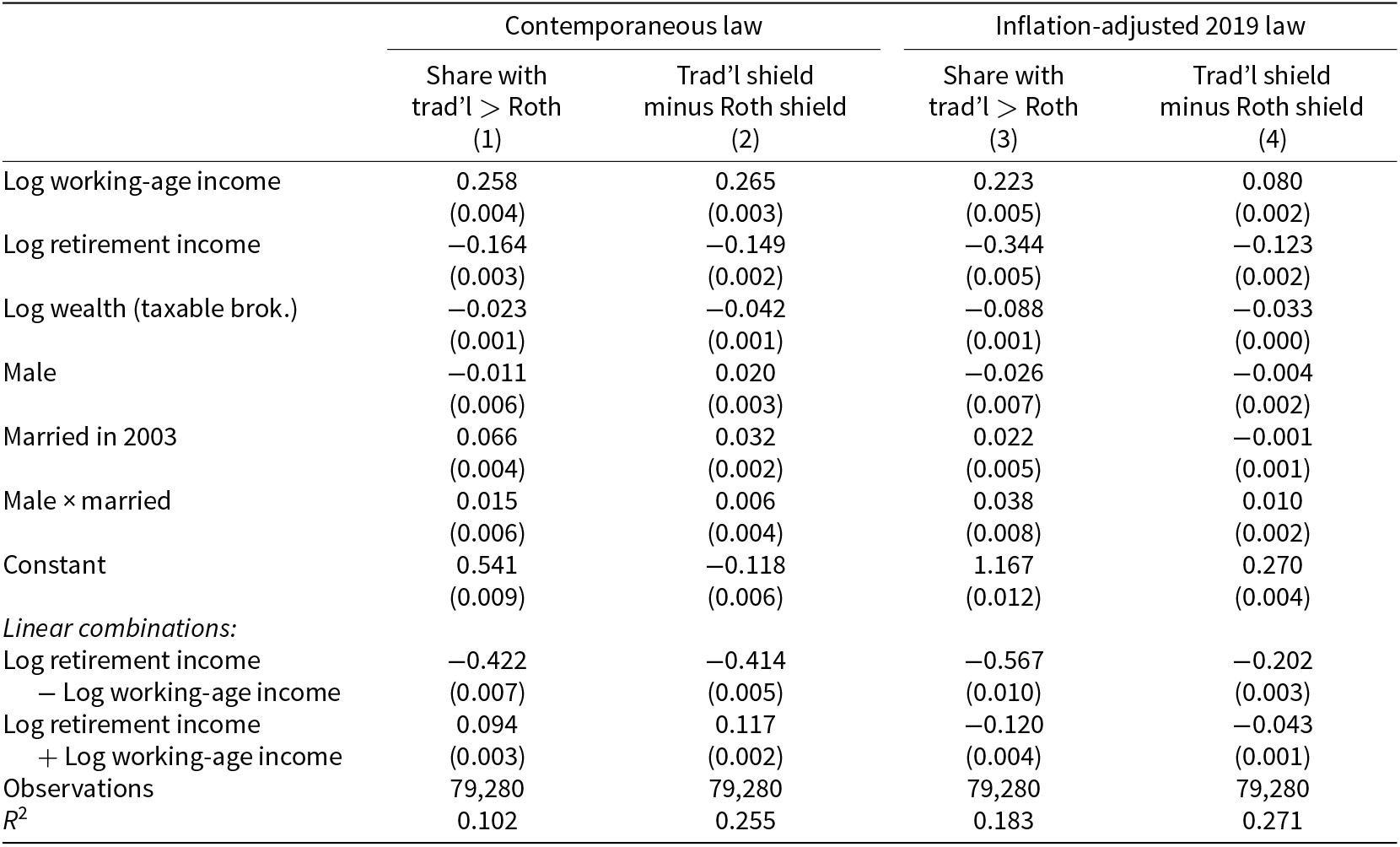
Notes: This table reports the coefficients from four regressions. The dependent variable in columns (1) and (3) is a dummy for an individual achieving more wealth in a traditional account than a Roth account. The dependent variable in columns (2) and (4) is the traditional shield minus the Roth shield. Income is defined as AGI, plus non-taxable social security income, minus taxable distributions from IRAs; for the purpose of this regression, we divide income by two in the case of married couples and we deem working age to begin at age 25. Near the bottom of the table, we report two sets of linear combinations of these regression coefficients that are of economic interest. The difference in the coefficients on log retirement income and log working-age income represents the implied effect of the log of the replacement rate. The sum of the coefficients on log retirement income and log working-age income represents the implied effect of a proportional increase in income during both retirement and working-age. Standard errors in parentheses.

Columns (1) and (2) use contemporaneous law, while columns (3) and (4) use inflation-adjusted 2019 law; columns (1) and (3) use the binary dependent variable while columns (2) and (4) use the difference between the traditional tax and the Roth tax shield. In all columns, there is a clear positive relationship between working age income and the relative advantage of traditional accounts; similarly, there is a clear negative relationship between retirement income and the relative advantage of traditional accounts. This result is unsurprising: a worker with higher working-age income will tend to face a higher working-age marginal tax rate (making traditional accounts more preferable), while a worker with higher retirement-age income will tend to face a higher retirement-age marginal tax rate (making traditional accounts less preferable).

Two transformations of these regression coefficients are of interest; these transformations are reported at the bottom of Table 5. First, the difference between the coefficient on retirement-age income and the coefficient on working-age income reflects the implied effect of the log of the replacement rate‒that is, the ratio of retirement-age income to working-age income. The effect is strongly negative: those with a larger replacement rate will tend to prefer Roth accounts, as their marginal rate in retirement will tend to be larger than their marginal rate in working age. Second, the sum of the two coefficients reflects the implied effect of increasing both retirement-age and working-age income proportionally. Here, we find a difference between contemporaneous law and inflation-adjusted 2019 law. Under inflation-adjusted 2019 law, such a proportional increase in income throughout life tends to make Roth accounts more preferred, while the reverse is true under contemporaneous law.

Next, we see that higher savings‒holding income fixed‒makes Roth accounts relatively more favorable. This likely reflects the fact that a larger account balance creates larger distributions, which has the effect of pushing people into higher tax brackets. We find that demographic variables (gender and marital status) have relatively more modest effects.

In Figure 3, we show the effect of the replacement rate in more detail. We plot the Roth and traditional shields (both relative to taxable accounts) and the share of individuals achieving more wealth in traditional accounts in 15 bins of the replacement rate. Under both legal counterfactuals, we see the clear negative effect on the relative advantage of traditional accounts. Under inflation-adjusted 2019 law (right panel), the indifference point occurs at a replacement rate of approximately one, with larger replacement-rate individuals preferring Roth accounts and lower replacement-rate individuals preferring traditional accounts. By contrast, under contemporaneous law (left panel), the individuals with the largest replacement rate still tend to prefer traditional accounts over Roth accounts‒that is, the reduction in marginal tax rates caused by changes in the tax schedule is enough to overcome the increase in marginal rate caused by increased income.

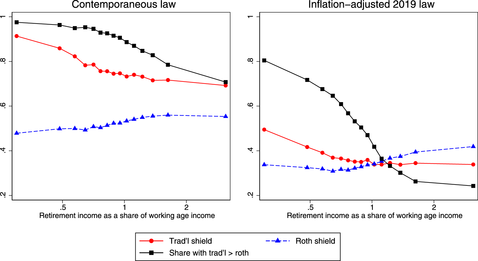
Figure 3. Heterogeneity by replacement rate.

Notes: This figure plots the average traditional shield, average Roth shield, and the share of individuals that achieve more wealth in traditional accounts as a function of the replacement rate. The replacement rate is defined as retirement-age income divided by working-age income. Retirement-age is defined to begin in 2003. Working-age is defined to begin at age 25 and end in 2002. Income is defined as AGI plus non-taxable social security income, with this entire quantity divided by two when the individual is part of a jointly filing married couple.

5.3. Extension: Contributions at maximum

In our baseline analysis, we have abstracted from contribution limits. However, for a saver who is constrained by contribution limits, Roth accounts effectively allow savers to shelter more (after-tax-equivalent) savings than traditional accounts. This occurs because the same contribution limits apply to traditional and Roth accounts even though traditional contributions are before-tax and Roth contributions are after-tax. This advantage to Roth accounts has been eliminated by assumption in our baseline analysis.

In this section, we quantify this advantage under the extreme assumption that each individual in our sample saved an amount equivalent to contributing the maximum to a Roth IRA in every year from 1975 through 2002.²⁷ These results are presented in Table 6, which quantifies the advantage of Roth accounts caused by the effectively higher contribution limits.

Table 6. Wealth if saving at maximum IRA limit

Notes: This table reports the wealth achieved when individuals save an amount equivalent to the maximum Roth IRA contribution in each year. The table contemplates three alternative savings strategies: (1) save in Roth, (2) save up to the contribution limit in traditional accounts and save the remainder in taxable brokerage accounts, and (3) save in taxable brokerage accounts. Under contemporaneous law, we use the nominal contemporaneous IRA limit, which is zero prior to 1975. Under inflation-adjusted 2019 law, we use the 2019 limit adjusted for inflation. The limit includes catch-up limits, where applicable. We additionally restrict that individuals do not save more than their net-of-tax wages.

On average, individuals would have accumulated an account balance of $223,000 under contemporaneous law or $363,000 under inflation-adjusted 2019 law. Holding fixed the individual’s after-tax savings, that individual could have contributed at the maximum to a traditional IRA in each of those years and still had some excess savings because contributions to a traditional IRA are on a before-tax basis. If those excess savings were put into a taxable account, then we estimate the balance in the taxable account at retirement would have been $42,000 under contemporaneous law or $48,000 under inflation-adjusted 2019 law. We estimate the present value of retirement consumption financed through the traditional IRA and brokerage account combined would have been $201,000 (contemporaneous law) or $311,000 (inflation-adjusted 2019 law). This is around 10 percent (contemporaneous law) or 14 percent (inflation-adjusted 2019 law) less than retirement consumption financed through the Roth IRA. We find that 92 percent (contemporaneous law) or 98 percent (inflation-adjusted 2019 law) of individuals achieve more retirement wealth saving in Roth relative to traditional accounts. Thus, even under contemporaneous law when the general patterns of marginal tax rates strongly favor traditional accounts, the ability to shelter more effective savings from tax on investment returns causes Roth accounts to usually be favored when contribution limits are always binding.

That said, the vast majority of savers tend not to be constrained by contribution limits in practice. Using an auxiliary sample of individuals in 2005 who were between the ages of 25 and 54, we find that only 14 percent of savers were constrained by such limits.²⁸ Thus, while contribution limits tend to cause Roth accounts to be favored for those for whom it is binding, we find that this consideration is relevant only for a small slice of savers.

6. Discussion and conclusion

In this paper, we used the 2003 cohort of retirees to examine the relative performance of traditional and Roth retirement accounts. Using administrative data and a detailed tax calculator, our analysis incorporates individual-level estimates of marginal tax rates throughout the lifetime.

Under contemporaneous law, we find that the vast majority of 2003 retirees would have been better off saving in traditional retirement accounts. For most of this cohort, the reduction in tax rates caused by tax changes in 1986, 2001, and 2003 tax rates enough that retirement-age marginal tax rates were lower than working-age marginal tax rates. Under inflation-adjusted 2019 law, we find that a slimmer majority of retirees would have been better off saving in traditional retirement accounts. About one third of the cohort would have been better off using Roth accounts under 2019 law. If there are no changes to federal tax law, we expect this scenario would be more informative for workers currently facing the choice between saving in traditional and Roth accounts. Traditional accounts tend to do better relative to Roth accounts when contributions are made later in working life and when distributions are taken later in retirement.

Our analysis faces several limitations. First, we abstract from bequests; if heirs face a higher marginal tax rate than retired individuals, that would tend to favor Roth accounts. Relatedly, the lack of bequests shuts down estate tax considerations which also tend to favor Roth accounts.

Second, we are holding real savings and investment decisions fixed when we compare account types. For instance, it may be the case that people would shift to more lightly taxed forms of investment (e.g., long-term capital gains) if forced to use a taxable account. This could cause us to overestimate the tax shield of both types of retirement accounts relative to taxable brokerage accounts. Additionally, it may be the case that behavioral biases cause people to save more in Roth accounts than traditional accounts – either because individuals desire to make a certain nominal contribution to a retirement account or because of confusion regarding the tax difference between Roth and traditional accounts (Adelman and Cross, 2010). Indeed, Beshears et al. (2017) find empirical support for this hypothesis: individuals tended to contribute the same amount to their employer-sponsored plan after the introduction of a Roth option, which means that savings effectively increased.

Third, our baseline analysis abstracts from contribution limits. If contribution limits are binding, individuals can effectively save more in a Roth account than they can in a traditional account. We have shown that these limits are sufficient to reverse the ranking between Roth and traditional accounts if they are always binding.

Fourth, our baseline analysis does not allow for more granular strategies regarding distributions. For instance, a retiree could strategically take distributions from traditional IRAs in years when marginal tax rates were low. Such a strategy would favor traditional accounts (or a mix of traditional and Roth).

Fifth, our analysis is entirely retrospective and assumes perfect foresight of investment returns and marginal tax rates. In reality, individuals face substantial uncertainty over these elements. Brown et al. (2017) showed that, under certain conditions, this uncertainty tends to favor Roth accounts because the value of traditional accounts is more uncertain due to uncertainty in retirement-age marginal tax rates. There are other conditions in which uncertainty favors traditional accounts. For instance, suppose that there is uncertainty over other sources of retirement income. Traditional accounts are more valuable exactly when individuals have a bad draw of other income; this ‘hedging’ property tends to favor traditional accounts.

Finally, and perhaps most substantively, the experience of the 2003 cohort of retirees may not match the experience of current working-age individuals. As DC saving was in its earlier stages for the 2003 cohort, these retirees may have been located in a different part of the income distribution than current working age individuals. Additionally, the 2003 cohort had greater access to defined benefit pensions, potentially increasing sources of other taxable income in retirement and thus increasing retirement-age marginal tax rates. Furthermore, income dynamics during working age may systematically differ between the two cohorts, perhaps most fundamentally for women. It is not obvious whether these factors, in sum, tend to favor Roth or traditional accounts – therefore, we think the empirical findings in this paper are still broadly informative for the current cohort, even if imperfect.

In the end, we find that many individuals could achieve a similar amount of wealth in traditional and Roth accounts under the inflation-adjusted 2019 law counterfactual. Thus, it is likely that many of these additional considerations which we have not formally modeled may be enough to sway a saver’s decision one way or the other. Future research should work to integrate these factors to help savers best prepare themselves for retirement.