


1. Introduction
The Wisconsin high-temperature superconductor axisymmetric mirror (WHAM) is a new laboratory experiment that confines hot plasmas in a magnetic mirror with a maximum field of $17\;\mathrm{T}$
on axis, generated by high-temperature superconductors (HTS) (Endrizzi et al. Reference Endrizzi2023). For WHAM and future mirror devices (Simonen et al. Reference Simonen2008; Bagryansky Reference Bagryansky2024; Forest et al. Reference Forest2024) to succeed, both fluid and kinetic plasma instabilities must be quelled.
$17\;\mathrm{T}$
on axis, generated by high-temperature superconductors (HTS) (Endrizzi et al. Reference Endrizzi2023). For WHAM and future mirror devices (Simonen et al. Reference Simonen2008; Bagryansky Reference Bagryansky2024; Forest et al. Reference Forest2024) to succeed, both fluid and kinetic plasma instabilities must be quelled.
A kinetic instability of particular concern is the drift-cyclotron loss-cone (DCLC) instability (Post & Rosenbluth Reference Post and Rosenbluth1966; Baldwin Reference Baldwin1977). The DCLC comprises a spectrum of ion Bernstein waves, coupled to a collisionless drift wave, which is excited by a spatial density gradient ${\nabla } n$
and a loss-cone ion velocity distribution. In a magnetized plasma column, DCLC appears as an electrostatic wave that propagates around the column’s azimuth in the ion diamagnetic drift direction, perpendicular to both
${\nabla } n$
and a loss-cone ion velocity distribution. In a magnetized plasma column, DCLC appears as an electrostatic wave that propagates around the column’s azimuth in the ion diamagnetic drift direction, perpendicular to both $\boldsymbol{B}$
and
$\boldsymbol{B}$
and ${\nabla } n$
. The DCLC can be unstable solely due to
${\nabla } n$
. The DCLC can be unstable solely due to ${\nabla } n$
when the gradient length scale
${\nabla } n$
when the gradient length scale $n/({\nabla } n)$
is of the order of the ion Larmor radius
$n/({\nabla } n)$
is of the order of the ion Larmor radius $\rho _{{i}}$
, even for distributions without a loss cone (e.g. Maxwellians), in which case it may be called a drift-cyclotron instability (Mikhailovskii & Timofeev Reference Mikhailovskii and Timofeev1963). In this manuscript, we call both drift-cyclotron and drift-cyclotron loss-cone modes by the acronym ‘DCLC’ for simplicity.
$\rho _{{i}}$
, even for distributions without a loss cone (e.g. Maxwellians), in which case it may be called a drift-cyclotron instability (Mikhailovskii & Timofeev Reference Mikhailovskii and Timofeev1963). In this manuscript, we call both drift-cyclotron and drift-cyclotron loss-cone modes by the acronym ‘DCLC’ for simplicity.
Many mirror devices have measured electric and/or magnetic fluctuations at discrete ion cyclotron harmonics having properties consistent with DCLC. These devices include PR-6 (Bajborodov et al. Reference Bajborodov, Ioffe, Kanaev, Sobolev and Jushmanov1971; Ioffe et al. Reference Ioffe, Kanaev, Pastukhov and Yushmanov1975), PR-8 (Piterskiǐ et al. Reference Piterskiǐ, Yushmanov and Yakovets1995), 2XIIB (Coensgen et al. Reference Coensgen, Cummins, Logan, Molvik, Nexsen, Simonen, Stallard and Turner1975), TMX and TMX-U (Drake et al. Reference Drake, Casper, Clauser, Coensgen, Correll, Cummins, Davis, Foote, Futch and Goodman1981; Simonen et al. Reference Simonen1983; Berzins & Casper Reference Berzins and Casper1987), LAMEX (Ferron & Wong Reference Ferron and Wong1984), MIX-1 (Koepke et al. Reference Koepke, Ellis, Majeski and McCarrick1986a
,
Reference Koepke, McCarrick, Majeski and Ellisb
; McCarrick et al. Reference McCarrick, Booske and Ellis1987; Burkhart et al. Reference Burkhart, Guzdar and Koepke1989), GAMMA-6A (Yamaguchi Reference Yamaguchi1996) and the gas dynamic trap (GDT) (Prikhodko et al. Reference Prikhodko2018; Shmigelsky et al. Reference Shmigelsky, Meyster, Chernoshtanov, Lizunov, Solomakhin and Yakovlev2024). Experiments on these devices showed that DCLC may be partly or wholly stabilized by filling the ions’ velocity-space loss cone via axial plasma stream injection (Ioffe et al. Reference Ioffe, Kanaev, Pastukhov and Yushmanov1975; Coensgen et al. Reference Coensgen, Cummins, Logan, Molvik, Nexsen, Simonen, Stallard and Turner1975; Kanaev Reference Kanaev1979; Correll et al. Reference Correll, Clauser, Coensgen, Cummins, Drake, Foote, Futch, Goodman, Grubb and Melin1980; Drake et al. Reference Drake, Casper, Clauser, Coensgen, Correll, Cummins, Davis, Foote, Futch and Goodman1981; Simonen et al. Reference Simonen1983; Berzins & Casper Reference Berzins and Casper1987), filling the loss cone via angled neutral beam injection, which creates a non-monotonic axial potential that traps cool ions (Kesner Reference Kesner1973, Reference Kesner1980; Fowler et al. Reference Fowler, Moir and Simonen2017; Shmigelsky et al. Reference Shmigelsky, Meyster, Chernoshtanov, Lizunov, Solomakhin and Yakovlev2024), decreasing ${\nabla } n$
with respect to the ion Larmor radius
${\nabla } n$
with respect to the ion Larmor radius $\rho _{{i}}$
(Ferron & Wong Reference Ferron and Wong1984) and bounce-resonant electron Landau damping (Koepke et al. Reference Koepke, Ellis, Majeski and McCarrick1986a
). Other effects theoretically calculated to modify and/or help stabilize DCLC include finite plasma beta (Tang et al. Reference Tang, Pearlstein and Berk1972), radial ambipolar electric fields (Chaudhry Reference Chaudhry1983; Sanuki & Ferraro Reference Sanuki and Ferraro1986) and low-frequency external electric fields (Aamodt Reference Aamodt1977; Hasegawa Reference Hasegawa1978).
$\rho _{{i}}$
(Ferron & Wong Reference Ferron and Wong1984) and bounce-resonant electron Landau damping (Koepke et al. Reference Koepke, Ellis, Majeski and McCarrick1986a
). Other effects theoretically calculated to modify and/or help stabilize DCLC include finite plasma beta (Tang et al. Reference Tang, Pearlstein and Berk1972), radial ambipolar electric fields (Chaudhry Reference Chaudhry1983; Sanuki & Ferraro Reference Sanuki and Ferraro1986) and low-frequency external electric fields (Aamodt Reference Aamodt1977; Hasegawa Reference Hasegawa1978).
The WHAM plasma column is a few to several ion Larmor radii ( $\rho _{{i}}$
) in width and so may excite DCLC. How will DCLC appear in WHAM; i.e. what will be its azimuthal mode number, oscillation frequency and amplitude? Sloshing ions, injected at
$\rho _{{i}}$
) in width and so may excite DCLC. How will DCLC appear in WHAM; i.e. what will be its azimuthal mode number, oscillation frequency and amplitude? Sloshing ions, injected at $45^\circ$
pitch-angle, helped to suppress DCLC in TMX-U endplugs and are also used on WHAM; to what extent can sloshing ions similarly suppress DCLC in WHAM? In general, how should WHAM’s plasma properties be tuned to suppress DCLC? These questions have been addressed to varying degrees, for previous devices, via linear theory (Post & Rosenbluth Reference Post and Rosenbluth1966; Tang et al. Reference Tang, Pearlstein and Berk1972; Gerver Reference Gerver1976; Lindgren et al. Reference Lindgren, Birdsall and Langdon1976; Baldwin Reference Baldwin1977; Cohen et al. Reference Cohen, Maron and Smith1982, Reference Cohen, Smith, Maron and Nevins1983; Ferraro et al. Reference Ferraro, Littlejohn, Sanuki and Fried1987; Kotelnikov et al. Reference Kotelnikov, Chernoshtanov and Prikhodko2017; Kotelnikov & Chernoshtanov Reference Kotelnikov and Chernoshtanov2018), quasilinear theory (Baldwin et al. Reference Baldwin, Berk and Pearlstein1976; Berk & Stewart Reference Berk and Stewart1977), nonlinear theory (Aamodt Reference Aamodt1977; Aamodt et al. Reference Aamodt1977; Myer & Simon Reference Myer and Simon1980) and one- and two-dimensional (2-D) kinetic computer simulations (Cohen & Maron Reference Cohen and Maron1980; Aamodt et al. Reference Aamodt, Cohen, Lee, Liu, Nicholson and Rosenbluth1981; Cohen et al. Reference Cohen, Maron and Smith1982, Reference Cohen, Smith, Maron and Nevins1983, Reference Cohen, Maron and Nevins1984; Rose et al. Reference Rose, Genoni, Welch, Mehlhorn, Porter and Ditmire2006).
$45^\circ$
pitch-angle, helped to suppress DCLC in TMX-U endplugs and are also used on WHAM; to what extent can sloshing ions similarly suppress DCLC in WHAM? In general, how should WHAM’s plasma properties be tuned to suppress DCLC? These questions have been addressed to varying degrees, for previous devices, via linear theory (Post & Rosenbluth Reference Post and Rosenbluth1966; Tang et al. Reference Tang, Pearlstein and Berk1972; Gerver Reference Gerver1976; Lindgren et al. Reference Lindgren, Birdsall and Langdon1976; Baldwin Reference Baldwin1977; Cohen et al. Reference Cohen, Maron and Smith1982, Reference Cohen, Smith, Maron and Nevins1983; Ferraro et al. Reference Ferraro, Littlejohn, Sanuki and Fried1987; Kotelnikov et al. Reference Kotelnikov, Chernoshtanov and Prikhodko2017; Kotelnikov & Chernoshtanov Reference Kotelnikov and Chernoshtanov2018), quasilinear theory (Baldwin et al. Reference Baldwin, Berk and Pearlstein1976; Berk & Stewart Reference Berk and Stewart1977), nonlinear theory (Aamodt Reference Aamodt1977; Aamodt et al. Reference Aamodt1977; Myer & Simon Reference Myer and Simon1980) and one- and two-dimensional (2-D) kinetic computer simulations (Cohen & Maron Reference Cohen and Maron1980; Aamodt et al. Reference Aamodt, Cohen, Lee, Liu, Nicholson and Rosenbluth1981; Cohen et al. Reference Cohen, Maron and Smith1982, Reference Cohen, Smith, Maron and Nevins1983, Reference Cohen, Maron and Nevins1984; Rose et al. Reference Rose, Genoni, Welch, Mehlhorn, Porter and Ditmire2006).
Here, we address the aforementioned questions using 3-D full-device computer simulations of DCLC growth and saturation in a hybrid (kinetic ion, fluid electron) plasma model. Our simulation accounts for many physical effects relevant to WHAM – magnetic geometry, beam-ion distributions, both radial and axial electrostatic potentials and diamagnetic field response – to obtain a fuller and more integrated kinetic model than was possible decades ago. We highlight that the initial beam-ion distributions are obtained from a Fokker–Planck collisional-transport model of a WHAM shot’s full $20 \;\mathrm{ms}$
duration. The Fokker–Planck modelling and code-coupling methods are presented by a companion study, Frank et al. (Reference Frank2025) within this journal issue.
$20 \;\mathrm{ms}$
duration. The Fokker–Planck modelling and code-coupling methods are presented by a companion study, Frank et al. (Reference Frank2025) within this journal issue.
In § 2 we describe our simulation methods and parameters. In §§ 3.1 to 3.3, we characterize three fiducial simulations evolved to $6 \;\mathrm{\unicode{x03BC}s}$
that have reached a steady-state decay. The main instability in all simulations is described and identified as DCLC, with the aid of an approximate linear dispersion relation for electrostatic waves in an inhomogeneous, low-
$6 \;\mathrm{\unicode{x03BC}s}$
that have reached a steady-state decay. The main instability in all simulations is described and identified as DCLC, with the aid of an approximate linear dispersion relation for electrostatic waves in an inhomogeneous, low- $\beta$
planar-slab plasma. In § 3.4, particle confinement is shown to obey a ‘gas dynamic’ rather than ‘collisionless mirror’ scaling with mirror ratio and device length. In §§ 4.1–4.3, we survey well-known ways to stabilize DCLC that may be relevant to WHAM and next-step mirror devices. We particularly focus on stabilization via trapped cool ions, and we show that adding cool ions can improve beam-ion confinement several-fold in our simulations. In §§ 4.4 and 4.5 we briefly discuss how DCLC in WHAM fits into a broader landscape of other instabilities and devices. Finally, § 5 concludes.
$\beta$
planar-slab plasma. In § 3.4, particle confinement is shown to obey a ‘gas dynamic’ rather than ‘collisionless mirror’ scaling with mirror ratio and device length. In §§ 4.1–4.3, we survey well-known ways to stabilize DCLC that may be relevant to WHAM and next-step mirror devices. We particularly focus on stabilization via trapped cool ions, and we show that adding cool ions can improve beam-ion confinement several-fold in our simulations. In §§ 4.4 and 4.5 we briefly discuss how DCLC in WHAM fits into a broader landscape of other instabilities and devices. Finally, § 5 concludes.
2. Methods
2.1. Simulation overview
We simulate freely decaying plasma in a three-dimensional (3-D) magnetic mirror made of one central cell and two expanders (figure 1
a,e,i). Three magnetic-field configurations are used, labelled by the vacuum mirror ratio $R_{{m}} = \{20, 41, 64\}$
, to span WHAM’s operating range. The WHAM magnetic field is created by two HTS coils at
$R_{{m}} = \{20, 41, 64\}$
, to span WHAM’s operating range. The WHAM magnetic field is created by two HTS coils at $z = \pm 98 \;\mathrm{cm}$
and two copper coils at
$z = \pm 98 \;\mathrm{cm}$
and two copper coils at $z = \pm 20 \;\mathrm{cm}$
(Endrizzi et al. 2023). When both HTS and copper coils are fully powered, the magnetic field on axis varies between
$z = \pm 20 \;\mathrm{cm}$
(Endrizzi et al. 2023). When both HTS and copper coils are fully powered, the magnetic field on axis varies between $B \approx 17.3 \;\mathrm{T}$
at the mirror throats to
$B \approx 17.3 \;\mathrm{T}$
at the mirror throats to $0.86 \;\mathrm{T}$
at the device’s centre (
$0.86 \;\mathrm{T}$
at the device’s centre ( $R_{{m}}=20$
). When the copper coils are partly powered,
$R_{{m}}=20$
). When the copper coils are partly powered, $B$
on axis ranges between
$B$
on axis ranges between $17.2$
to
$17.2$
to $0.414 \;\mathrm{T}$
(
$0.414 \;\mathrm{T}$
( $R_{{m}}=41$
). When the copper coils are unpowered,
$R_{{m}}=41$
). When the copper coils are unpowered, $B$
on axis ranges between
$B$
on axis ranges between $17.1$
to
$17.1$
to $0.267 \;\mathrm{T}$
(
$0.267 \;\mathrm{T}$
( $R_{{m}}=64$
).
$R_{{m}}=64$
).
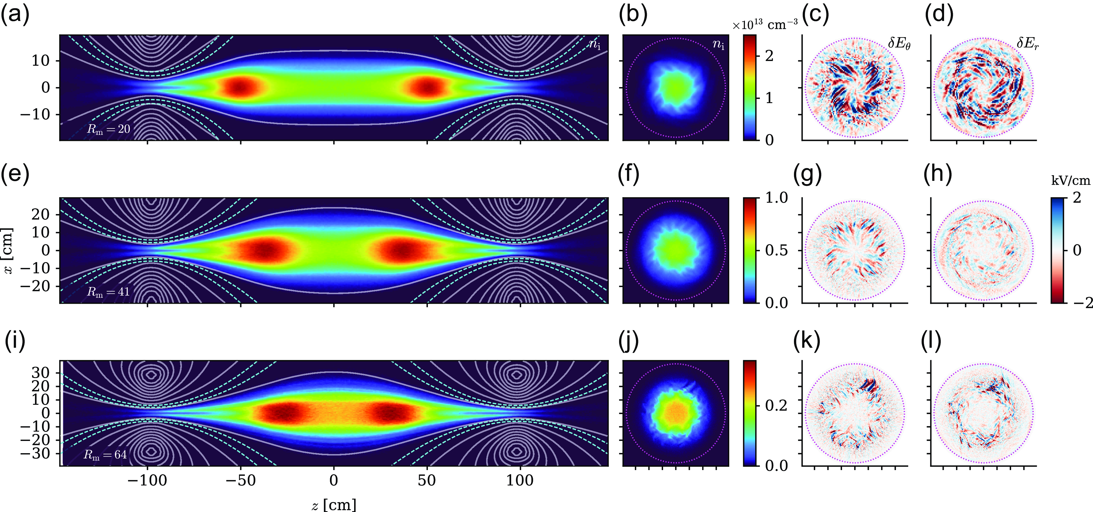
Figure 1. The 2-D images of ion density and electric field fluctuations at $t \approx 6 \tau _{\mathrm{bounce}} \approx 6 \mu s$
, for three simulations with varying vacuum mirror ratio (a–d)
$t \approx 6 \tau _{\mathrm{bounce}} \approx 6 \mu s$
, for three simulations with varying vacuum mirror ratio (a–d) $R_{{m}} = 20$
, (e–h)
$R_{{m}} = 20$
, (e–h) $41$
, (i–l)
$41$
, (i–l) $64$
. (a) Ion density
$64$
. (a) Ion density $n_{{i}}$
in units of
$n_{{i}}$
in units of $10^{13} \;\mathrm{cm^{-3}}$
, 2-D slice at
$10^{13} \;\mathrm{cm^{-3}}$
, 2-D slice at $y=0$
in
$y=0$
in $(x,y,z)$
coordinates. White lines trace vacuum magnetic fields; dashed cyan lines trace hyper-resistive dampers and conducting
$(x,y,z)$
coordinates. White lines trace vacuum magnetic fields; dashed cyan lines trace hyper-resistive dampers and conducting $E=0$
regions (see text). (b) Like (a), but 2-D slice at the mirror’s midplane
$E=0$
regions (see text). (b) Like (a), but 2-D slice at the mirror’s midplane $z=0$
showing coherent flute-like fluctuations at the plasma edge. (c) Azimuthal electric field fluctuation
$z=0$
showing coherent flute-like fluctuations at the plasma edge. (c) Azimuthal electric field fluctuation $\delta E_\theta$
in kV cm−1; magenta dotted line traces radial conducting boundary. (d) Like (c), but radial fluctuation
$\delta E_\theta$
in kV cm−1; magenta dotted line traces radial conducting boundary. (d) Like (c), but radial fluctuation $\delta E_r$
. Panels (e)–(h) and (i)–(l) are organized like panels (a)–(d). Aspect ratio is distorted in panels (a), (e) and (i); aspect ratio is to scale in all other panels. The ion bounce time
$\delta E_r$
. Panels (e)–(h) and (i)–(l) are organized like panels (a)–(d). Aspect ratio is distorted in panels (a), (e) and (i); aspect ratio is to scale in all other panels. The ion bounce time $\tau _{\mathrm{bounce}}$
is defined later in § 2.3.
$\tau _{\mathrm{bounce}}$
is defined later in § 2.3.
Our simulations are performed with the code Hybrid-VPICFootnote
1
(Le et al. Reference Le, Stanier, Yin, Wetherton, Keenan and Albright2023; Bowers et al. Reference Bowers, Albright, Yin, Bergen and Kwan2008), which models ion kinetics using the particle-in-cell (PIC) method and models electrons as a neutralizing fluid. Ions are advanced using a Boris pusher (Bowers et al. Reference Bowers, Albright, Yin, Bergen and Kwan2008). Electric and magnetic fields $\boldsymbol{E}$
,
$\boldsymbol{E}$
, $\boldsymbol{B}$
are evolved on a rectilinear Cartesian (
$\boldsymbol{B}$
are evolved on a rectilinear Cartesian ( $x,y,z$
) mesh. Particle–mesh interpolation uses a quadratic-sum shape (Le et al. Reference Le, Stanier, Yin, Wetherton, Keenan and Albright2023; Appendix B); no filtering of the deposited particle charge and currents is applied. The magnetic field is advanced using Faraday’s Law,
$x,y,z$
) mesh. Particle–mesh interpolation uses a quadratic-sum shape (Le et al. Reference Le, Stanier, Yin, Wetherton, Keenan and Albright2023; Appendix B); no filtering of the deposited particle charge and currents is applied. The magnetic field is advanced using Faraday’s Law, $\partial \boldsymbol{B}/\partial t = - c{\nabla } \times \boldsymbol{E}$
, with a fourth-order Runge–Kutta scheme. The electric field is passively set by a generalized Ohm’s law without electron inertia,
$\partial \boldsymbol{B}/\partial t = - c{\nabla } \times \boldsymbol{E}$
, with a fourth-order Runge–Kutta scheme. The electric field is passively set by a generalized Ohm’s law without electron inertia,
 \begin{equation} \boldsymbol{E} = - \frac {\boldsymbol{V}_{{i}} \times \boldsymbol{B}}{c} + \frac {\boldsymbol{j} \times \boldsymbol{B}}{e n_{{e}} c} - \frac {{\nabla } P_{{e}}}{e n_{{e}}} + \eta \boldsymbol{j} - \eta _{{H}} {\nabla }^2 \boldsymbol{j} ,\end{equation}
assuming both $\boldsymbol{j} = c {\nabla } \times \boldsymbol{B} / (4\pi )$
and
$\boldsymbol{j} = c {\nabla } \times \boldsymbol{B} / (4\pi )$
and $n_{{e}} = n_{{i}}$
. We further take
$n_{{e}} = n_{{i}}$
. We further take $P_e = n_e T_e$
, with
$P_e = n_e T_e$
, with $T_e$
constant in time and space (isothermal). Here
$T_e$
constant in time and space (isothermal). Here $n_{{i}}$
and
$n_{{i}}$
and $n_{{e}}$
are ion and electron number densities,
$n_{{e}}$
are ion and electron number densities, $\boldsymbol{V}_{{i}}$
is bulk ion velocity,
$\boldsymbol{V}_{{i}}$
is bulk ion velocity, $P_{{e}}$
is scalar electron pressure,
$P_{{e}}$
is scalar electron pressure, $\boldsymbol{j}$
is current density,
$\boldsymbol{j}$
is current density, $\eta$
is resistivity,
$\eta$
is resistivity, $\eta _{{H}}$
is hyper-resistivity,
$\eta _{{H}}$
is hyper-resistivity, $c$
is the speed of light and
$c$
is the speed of light and $e$
is the elementary charge. Gaussian CGS units are used in this manuscript unless otherwise stated.
$e$
is the elementary charge. Gaussian CGS units are used in this manuscript unless otherwise stated.
Coulomb collisions are neglected because the ion–ion deflection and ion–electron drag time scales in the plasmas modeled here are of order ${O}(\mathrm{ms})$
, longer than our simulation durations
${O}(\mathrm{ms})$
, longer than our simulation durations $\mathord {\sim } 1$
–
$\mathord {\sim } 1$
– $10 \;\mathrm{\unicode{x03BC}s}$
.
$10 \;\mathrm{\unicode{x03BC}s}$
.
The hybrid-PIC equations solved here are non-relativistic: the displacement current $\partial \boldsymbol{E}/\partial t/(4\pi )$
is omitted from Ampére’s law, and no Lorentz factors are used in the Boris push. The speed of light is effectively infinite. All code equations are solved in a dimensionless form; the normalizations for converting code variables into physical units are set by choosing reference values of density, magnetic field, and ion species’ mass and charge.
$\partial \boldsymbol{E}/\partial t/(4\pi )$
is omitted from Ampére’s law, and no Lorentz factors are used in the Boris push. The speed of light is effectively infinite. All code equations are solved in a dimensionless form; the normalizations for converting code variables into physical units are set by choosing reference values of density, magnetic field, and ion species’ mass and charge.
A density floor of $n_{{e}} \geqslant \{15, 6, 1.5\} \times 10^{11} \;\mathrm{cm^{-3}}$
, for the
$n_{{e}} \geqslant \{15, 6, 1.5\} \times 10^{11} \;\mathrm{cm^{-3}}$
, for the $R_{{m}} = \{20, 41, 64\}$
simulations, respectively, is applied in the Hall and ambipolar (pressure gradient) terms of (2.1) to prevent division-by-zero in vacuum and low-density regions surrounding the plasma. The density floor is set low enough to obtain the electrostatic potential drop from
$R_{{m}} = \{20, 41, 64\}$
simulations, respectively, is applied in the Hall and ambipolar (pressure gradient) terms of (2.1) to prevent division-by-zero in vacuum and low-density regions surrounding the plasma. The density floor is set low enough to obtain the electrostatic potential drop from $z=0$
out to the mirror throats at
$z=0$
out to the mirror throats at $z = \pm 98\;\mathrm{cm}$
, but the remaining potential drop from throat into expanders is not captured. Lowering the density floor increases compute cost, so we sacrifice physics in the expanders that is less-accurately described by the hybrid-PIC model anyways.
$z = \pm 98\;\mathrm{cm}$
, but the remaining potential drop from throat into expanders is not captured. Lowering the density floor increases compute cost, so we sacrifice physics in the expanders that is less-accurately described by the hybrid-PIC model anyways.
The simulation time step $\Delta t$
must be smaller than a Courant–Friedrichs–Lewy (CFL) limit to resolve gridscale whistler waves:
$\Delta t$
must be smaller than a Courant–Friedrichs–Lewy (CFL) limit to resolve gridscale whistler waves: $\Delta t \propto n (\Delta z)^2 / B$
for cell size
$\Delta t \propto n (\Delta z)^2 / B$
for cell size $\Delta z$
less than the ion skin depth. The density floor in high-
$\Delta z$
less than the ion skin depth. The density floor in high- $\boldsymbol{B}$
vacuum regions thus sets the overall simulation time step. The CFL-limited time step is well below the ion-cyclotron period and other physical time scales of interest, so we subcycle the magnetic-field update
$\boldsymbol{B}$
vacuum regions thus sets the overall simulation time step. The CFL-limited time step is well below the ion-cyclotron period and other physical time scales of interest, so we subcycle the magnetic-field update $N_{\mathrm{sub}}$
times within each particle push to reduce compute cost. The CFL limit then applies to
$N_{\mathrm{sub}}$
times within each particle push to reduce compute cost. The CFL limit then applies to $\Delta t/ N_{\mathrm{sub}}$
, and larger
$\Delta t/ N_{\mathrm{sub}}$
, and larger $\Delta t$
can be used.
$\Delta t$
can be used.
We set the resistivity $\eta = 0$
and the hyper-resistivity
$\eta = 0$
and the hyper-resistivity $\eta _{{H}} = 2.75 \times 10^{-14} \;\mathrm{s\,cm^2}$
. Hyper-resistivity is used solely to damp high-frequency whistler noise at the grid scale
$\eta _{{H}} = 2.75 \times 10^{-14} \;\mathrm{s\,cm^2}$
. Hyper-resistivity is used solely to damp high-frequency whistler noise at the grid scale $k \sim \pi /\Delta z$
;
$k \sim \pi /\Delta z$
; $\eta _{{H}}$
does not represent any subgrid physics of interest to us. The hyper-resistive
$\eta _{{H}}$
does not represent any subgrid physics of interest to us. The hyper-resistive $\boldsymbol{E}$
is included in the ion push, since it is not used to model electron–ion friction.Footnote
2
Hyper-resistivity is the only explicit form of numerical dissipation in our simulations
$\boldsymbol{E}$
is included in the ion push, since it is not used to model electron–ion friction.Footnote
2
Hyper-resistivity is the only explicit form of numerical dissipation in our simulations
2.2. Simulation geometry
The simulation domain for the $R_{{m}}=20$
case is a rectangular box with extent
$R_{{m}}=20$
case is a rectangular box with extent $L_x = L_y = 39.2 \;\mathrm{cm}$
and
$L_x = L_y = 39.2 \;\mathrm{cm}$
and $L_z = 294 \;\mathrm{cm}$
. The box is decomposed into a
$L_z = 294 \;\mathrm{cm}$
. The box is decomposed into a $96^2 \times 384$
Cartesian
$96^2 \times 384$
Cartesian $(x,y,z)$
mesh with cell dimensions
$(x,y,z)$
mesh with cell dimensions $\Delta x = \Delta y = 0.41 \;\mathrm{cm}$
and
$\Delta x = \Delta y = 0.41 \;\mathrm{cm}$
and $\Delta z = 0.77 \;\mathrm{cm}$
. For analysis and discussion, we project data into usual cylindrical coordinates
$\Delta z = 0.77 \;\mathrm{cm}$
. For analysis and discussion, we project data into usual cylindrical coordinates $(r,\theta ,z)$
. For the
$(r,\theta ,z)$
. For the $R_{{m}} = 41$
and
$R_{{m}} = 41$
and $64$
cases, the domain is enlarged to
$64$
cases, the domain is enlarged to $L_x = L_y = 58.8$
and
$L_x = L_y = 58.8$
and $78.4 \;\mathrm{cm}$
respectively while preserving the mesh cell shape, so the number of mesh points is
$78.4 \;\mathrm{cm}$
respectively while preserving the mesh cell shape, so the number of mesh points is $144^2 \times 384$
and
$144^2 \times 384$
and $192^2 \times 384$
, respectively. The domain extent truncates the expanders at
$192^2 \times 384$
, respectively. The domain extent truncates the expanders at $z = \pm 147 \;\mathrm{cm}$
, unlike the real experiment, wherein a set of staggered biasable rings collects escaping plasma at
$z = \pm 147 \;\mathrm{cm}$
, unlike the real experiment, wherein a set of staggered biasable rings collects escaping plasma at $z \sim 190$
–
$z \sim 190$
– $210 \;\mathrm{cm}$
(Endrizzi et al. Reference Endrizzi2023; Qian et al. Reference Qian, Anderson, Endrizzi, Forest, Pizzo, Sanwalka, Yakovlev, Yu and Zarnstorff2023).
$210 \;\mathrm{cm}$
(Endrizzi et al. Reference Endrizzi2023; Qian et al. Reference Qian, Anderson, Endrizzi, Forest, Pizzo, Sanwalka, Yakovlev, Yu and Zarnstorff2023).
The overall simulation time step $\Delta t = 7.3 \times 10^{-11} \;\mathrm{s}$
. The magnetic-field advance is subcycled
$\Delta t = 7.3 \times 10^{-11} \;\mathrm{s}$
. The magnetic-field advance is subcycled $N_{\mathrm{sub}} = \{100, 250, 1000\}$
times within
$N_{\mathrm{sub}} = \{100, 250, 1000\}$
times within $\Delta t$
, for
$\Delta t$
, for $R_{{m}} = \{20, 41, 64\}$
, respectively.
$R_{{m}} = \{20, 41, 64\}$
, respectively.
Hyper-resistivity $\eta _{{H}}$
acts like smoothing and removes gridscale numerical noise on the whistler-wave dispersion branch, which would otherwise be undamped in the absence of resistivity or hyper-resistivity. The value of
$\eta _{{H}}$
acts like smoothing and removes gridscale numerical noise on the whistler-wave dispersion branch, which would otherwise be undamped in the absence of resistivity or hyper-resistivity. The value of $\eta _{{H}}$
must be kept small enough to not artificially smooth real physical phenomena. The hyper-resistive diffusion time scale estimated as
$\eta _{{H}}$
must be kept small enough to not artificially smooth real physical phenomena. The hyper-resistive diffusion time scale estimated as $\left [\eta _{{H}} c^2 / (4\pi L^4)\right ]^{-1}$
for an arbitrary length scale
$\left [\eta _{{H}} c^2 / (4\pi L^4)\right ]^{-1}$
for an arbitrary length scale $L$
is
$L$
is $1.4 \times 10^{-8} \;\mathrm{s}$
for the transverse grid scale
$1.4 \times 10^{-8} \;\mathrm{s}$
for the transverse grid scale $L \sim \Delta x$
; it is
$L \sim \Delta x$
; it is $600 \;\mathrm{\unicode{x03BC}s}$
for the ion skin depth
$600 \;\mathrm{\unicode{x03BC}s}$
for the ion skin depth $L \sim c/\omega _{\mathrm{pi}} \sim 6 \;\mathrm{cm}$
with
$L \sim c/\omega _{\mathrm{pi}} \sim 6 \;\mathrm{cm}$
with $n \sim 3 \times 10^{13} \;\mathrm{cm^{-3}}$
. We cannot make
$n \sim 3 \times 10^{13} \;\mathrm{cm^{-3}}$
. We cannot make $\eta _{{H}}$
much larger because the scale separation between grid noise and physical phenomena is small; high-
$\eta _{{H}}$
much larger because the scale separation between grid noise and physical phenomena is small; high- $m$
kinetic modes lie below the ion skin depth. In Appendix A, we present density fluctuation properties from a three-point scan of
$m$
kinetic modes lie below the ion skin depth. In Appendix A, we present density fluctuation properties from a three-point scan of $\eta _{{H}}$
; some details (e.g. spectral bandwidth) are altered, but the main conclusions regarding DCLC are not too sensitive to our chosen value of
$\eta _{{H}}$
; some details (e.g. spectral bandwidth) are altered, but the main conclusions regarding DCLC are not too sensitive to our chosen value of $\eta _{{H}}$
.
$\eta _{{H}}$
.
Particle and field boundary conditions are imposed as follows. A conducting radial sidewall is placed at $r = 0.47 L_x$
, which is in physical units
$r = 0.47 L_x$
, which is in physical units $\{18.4, 27.6, 36.8\} \;\mathrm{cm}$
for
$\{18.4, 27.6, 36.8\} \;\mathrm{cm}$
for $R_{{m}}=\{20,41,64\}$
, respectively. A conducting axial sidewall is placed at
$R_{{m}}=\{20,41,64\}$
, respectively. A conducting axial sidewall is placed at $z = 0.485 L_z = \pm 143 \;\mathrm{cm}$
. The HTS coils are also surrounded by both conducting and hyper-resistive wrapper layers (figure 1
a,e,i, dashed cyan curves). Within the wrapper layer (between nested dashed cyan curves), the grid-local value of
$z = 0.485 L_z = \pm 143 \;\mathrm{cm}$
. The HTS coils are also surrounded by both conducting and hyper-resistive wrapper layers (figure 1
a,e,i, dashed cyan curves). Within the wrapper layer (between nested dashed cyan curves), the grid-local value of $\eta _{{H}}$
used in Ohm’s law (2.1) is increased
$\eta _{{H}}$
used in Ohm’s law (2.1) is increased $30\times$
to help suppress numerical noise in high-field, low-density regions. The ‘conducting’ boundary is enforced by setting
$30\times$
to help suppress numerical noise in high-field, low-density regions. The ‘conducting’ boundary is enforced by setting $\boldsymbol{E} = 0$
on the mesh, which disables
$\boldsymbol{E} = 0$
on the mesh, which disables $\boldsymbol{B}$
field evolution. Bound charge and image currents within conducting surfaces are not explicitly modelled. Particles crossing the Cartesian domain boundaries (
$\boldsymbol{B}$
field evolution. Bound charge and image currents within conducting surfaces are not explicitly modelled. Particles crossing the Cartesian domain boundaries ( $x = \pm L_x/2$
,
$x = \pm L_x/2$
, $y = \pm L_y/2$
,
$y = \pm L_y/2$
, $z=\pm L_z/2$
) are removed from the simulation. Boundary conditions are applied to
$z=\pm L_z/2$
) are removed from the simulation. Boundary conditions are applied to $\boldsymbol{E}$
at cell centres in a nearest-gridpoint manner, which may contribute to mesh imprinting; boundaries might be improved with a cut-cell algorithm or simply higher grid resolution in future work.
$\boldsymbol{E}$
at cell centres in a nearest-gridpoint manner, which may contribute to mesh imprinting; boundaries might be improved with a cut-cell algorithm or simply higher grid resolution in future work.

Figure 2. Axial profiles of $n_{{i}}$
,
$n_{{i}}$
, $B$
,
$B$
, $\phi$
measured at
$\phi$
measured at $t = 6 \tau _{\mathrm{bounce}} \approx 6 \mathrm{\unicode{x03BC}s}$
. (a) Ion density
$t = 6 \tau _{\mathrm{bounce}} \approx 6 \mathrm{\unicode{x03BC}s}$
. (a) Ion density $n_{{i}}$
on axis (
$n_{{i}}$
on axis ( $r=0$
). Dashes mark density floor for Ohm’s law, (2.1). (b) Like (a), but measured along off-axis flux surfaces. (c) Magnetic-field strength
$r=0$
). Dashes mark density floor for Ohm’s law, (2.1). (b) Like (a), but measured along off-axis flux surfaces. (c) Magnetic-field strength $B$
on axis. Ions with
$B$
on axis. Ions with $45^\circ$
pitch angle turn where the local mirror ratio
$45^\circ$
pitch angle turn where the local mirror ratio $R_{{m}}(z)=2$
(triangles). (d) Electrostatic potential
$R_{{m}}(z)=2$
(triangles). (d) Electrostatic potential $e\phi$
in units of electron temperature
$e\phi$
in units of electron temperature $T_{{e}}$
, measured on-axis (thick curves) and off-axis (thin curves). Potentials truncate at
$T_{{e}}$
, measured on-axis (thick curves) and off-axis (thin curves). Potentials truncate at $z \sim 100\;\mathrm{cm}$
, corresponding to density floors marked in (a) and (b). In all panels: blue, orange, green curves are simulations with vacuum
$z \sim 100\;\mathrm{cm}$
, corresponding to density floors marked in (a) and (b). In all panels: blue, orange, green curves are simulations with vacuum $R_{{m}} = \{20, 41, 64\}$
, respectively; small triangles mark on-axis turning points
$R_{{m}} = \{20, 41, 64\}$
, respectively; small triangles mark on-axis turning points $R_{{m}}(z) = 2$
(coloured) and mirror throat (black).
$R_{{m}}(z) = 2$
(coloured) and mirror throat (black).
2.3. Plasma parameters
We model a fully ionized deuteron–electron plasma ( $m_{{i}} = 3.34\times 10^{-24}\;\mathrm{g}$
) with typical ion density
$m_{{i}} = 3.34\times 10^{-24}\;\mathrm{g}$
) with typical ion density $n_{{i}} \sim 10^{12}$
to
$n_{{i}} \sim 10^{12}$
to $10^{13} \;\mathrm{cm^{-3}}$
and temperature
$10^{13} \;\mathrm{cm^{-3}}$
and temperature $T_{{i}} \sim 5$
to
$T_{{i}} \sim 5$
to $13 \;\mathrm{keV}$
in the mirror’s central cell. The ion velocity distribution is a beam slowing-down distribution with pitch angle
$13 \;\mathrm{keV}$
in the mirror’s central cell. The ion velocity distribution is a beam slowing-down distribution with pitch angle $\cos ^{-1}(v_\parallel /v) \sim 45^\circ$
at the mirror midplane (
$\cos ^{-1}(v_\parallel /v) \sim 45^\circ$
at the mirror midplane ( $z=0$
) to mimic WHAM’s angled neutral beam injection (NBI). The beam path is centred on axis (
$z=0$
) to mimic WHAM’s angled neutral beam injection (NBI). The beam path is centred on axis ( $r=0$
).
$r=0$
).
The ions’ spatial and velocity distributions are obtained from the bounce-averaged, zero-orbit-width, collisional Fokker–Planck code CQL3D-m (Petrov & Harvey Reference Petrov and Harvey2016; Forest et al. Reference Forest2024). We initialize the CQL3D-m simulations with a $1.5 \times 10^{13} \;\mathrm{cm^{-3}}$
plasma at low temperature
$1.5 \times 10^{13} \;\mathrm{cm^{-3}}$
plasma at low temperature $T_i = T_e = 250 \;\mathrm{eV}$
, mimicking the initial electron-cyclotron heating (ECH) breakdown of a gas puff in WHAM.Footnote
3
The plasma is simulated by CQL3D-m on 32 flux surfaces spanning normalized square root poloidal flux,
$T_i = T_e = 250 \;\mathrm{eV}$
, mimicking the initial electron-cyclotron heating (ECH) breakdown of a gas puff in WHAM.Footnote
3
The plasma is simulated by CQL3D-m on 32 flux surfaces spanning normalized square root poloidal flux, $\sqrt {\psi _n} = 0.01$
–
$\sqrt {\psi _n} = 0.01$
– $0.9$
, as it is fuelled and heated with a realistic
$0.9$
, as it is fuelled and heated with a realistic $25 \;\mathrm{keV}$
neutral beam operating at the experimental parameters. No heating or fuelling sources other than the neutral beam are included. The velocity-space grid has 300 points in total momentum-per-rest-mass
$25 \;\mathrm{keV}$
neutral beam operating at the experimental parameters. No heating or fuelling sources other than the neutral beam are included. The velocity-space grid has 300 points in total momentum-per-rest-mass $p/(m c)$
, and either 256 or 300 points in pitch angle. The total-momentum grid is not linearly spaced, but instead geometrically scaled at low energies to cover the ion distribution function. The pitch-angle grid is uniformly spaced. The solver CQL3D-m uses a time step of
$p/(m c)$
, and either 256 or 300 points in pitch angle. The total-momentum grid is not linearly spaced, but instead geometrically scaled at low energies to cover the ion distribution function. The pitch-angle grid is uniformly spaced. The solver CQL3D-m uses a time step of $0.0625 \;\mathrm{ms}$
, advancing ions and electrons simultaneously. The neutral beam deposition profile is updated after each time step using the CQL3D-m internal FREYA neutral-beam Monte Carlo solver. To include the diamagnetic
$0.0625 \;\mathrm{ms}$
, advancing ions and electrons simultaneously. The neutral beam deposition profile is updated after each time step using the CQL3D-m internal FREYA neutral-beam Monte Carlo solver. To include the diamagnetic $\boldsymbol{B}$
-field response to the plasma pressure, the CQL3D-m solver is iterated with the MHD equilibrium solver PleiadesFootnote
4
(Peterson Reference Peterson2019), with improvements to treat pressure-anisotropic equilibria (Frank et al. Reference Frank2025). The CQL3D-m and Pleiades solvers are coupled using a customized version of the integrated plasma simulator framework (Elwasif et al. Reference Elwasif, Bernholdt, Shet, Foley, Bramley, Batchelor, Berry, Marco, Bourgeois and Gross2010). The diamagnetic field is updated in CQL3D-m every
$\boldsymbol{B}$
-field response to the plasma pressure, the CQL3D-m solver is iterated with the MHD equilibrium solver PleiadesFootnote
4
(Peterson Reference Peterson2019), with improvements to treat pressure-anisotropic equilibria (Frank et al. Reference Frank2025). The CQL3D-m and Pleiades solvers are coupled using a customized version of the integrated plasma simulator framework (Elwasif et al. Reference Elwasif, Bernholdt, Shet, Foley, Bramley, Batchelor, Berry, Marco, Bourgeois and Gross2010). The diamagnetic field is updated in CQL3D-m every $1 \;\mathrm{ms}$
.
$1 \;\mathrm{ms}$
.
We perform separate CQL3D-m runs for each of the $R_{{m}}=\{20,41,64\}$
cases. In each case, the NBI power is adjusted in
$R_{{m}}=\{20,41,64\}$
cases. In each case, the NBI power is adjusted in $100 \;\mathrm{kW}$
increments, until the
$100 \;\mathrm{kW}$
increments, until the $1 \;\mathrm{MW}$
maximum input power of the experiment is reached or a mirror instability driven
$1 \;\mathrm{MW}$
maximum input power of the experiment is reached or a mirror instability driven $\beta$
limit occurs (Kotelnikov Reference Kotelnikov2025). The
$\beta$
limit occurs (Kotelnikov Reference Kotelnikov2025). The $R_{{m}}=\{20,41,64\}$
cases operate with NBI power
$R_{{m}}=\{20,41,64\}$
cases operate with NBI power $\{200,400,1000\} \;\mathrm{kW}$
, respectively. The CQL3D-m/Pleiades loop is run for the duration of a laboratory shot, to
$\{200,400,1000\} \;\mathrm{kW}$
, respectively. The CQL3D-m/Pleiades loop is run for the duration of a laboratory shot, to $20 \;\mathrm{ms}$
(which is
$20 \;\mathrm{ms}$
(which is $t=0$
for Hybrid-VPIC). At the end of the CQL3D-m run, all three cases have plasma
$t=0$
for Hybrid-VPIC). At the end of the CQL3D-m run, all three cases have plasma $\beta \sim 0.60$
. The low
$\beta \sim 0.60$
. The low $R_{{m}}=20$
(high
$R_{{m}}=20$
(high $\boldsymbol{B}$
-field) case achieves the highest plasma density
$\boldsymbol{B}$
-field) case achieves the highest plasma density $1$
–
$1$
– $3 \times 10^{13} \;\mathrm{cm^{-3}}$
on axis in the central cell (figure 2
a). The ions have
$3 \times 10^{13} \;\mathrm{cm^{-3}}$
on axis in the central cell (figure 2
a). The ions have $T_{{i}} = \{13, 11, 11\} \;\mathrm{keV}$
at the origin
$T_{{i}} = \{13, 11, 11\} \;\mathrm{keV}$
at the origin $(r,z)=(0,0)$
in the
$(r,z)=(0,0)$
in the $R_{{m}}=\{20,41,64\}$
cases, respectively. Of note, the
$R_{{m}}=\{20,41,64\}$
cases, respectively. Of note, the $R_{{m}}=64$
case has a cooler ion plasma temperature
$R_{{m}}=64$
case has a cooler ion plasma temperature $T_{{i}} \sim 5 \;\mathrm{keV}$
at the plasma’s radial edge, whereas the lower
$T_{{i}} \sim 5 \;\mathrm{keV}$
at the plasma’s radial edge, whereas the lower $R_{{m}}$
(higher field) CQL3D-m simulations maintain
$R_{{m}}$
(higher field) CQL3D-m simulations maintain $T_{{i}} \sim 10 \;\mathrm{keV}$
from the axis
$T_{{i}} \sim 10 \;\mathrm{keV}$
from the axis $r=0$
to the edge. This is a result of the larger cool thermal ion population that is trapped by the sloshing-ion distribution in the
$r=0$
to the edge. This is a result of the larger cool thermal ion population that is trapped by the sloshing-ion distribution in the $R_{{m}}=64$
case.
$R_{{m}}=64$
case.
The CQL3D-m bounce-averaged distribution function at the mirror’s midplane ( $z=0$
) is mapped on Liouville characteristics to all (
$z=0$
) is mapped on Liouville characteristics to all ( $r,z$
) and read into Hybrid-VPIC as an initial condition for both real- and velocity-space ion distributions. The CQL3D-m ion radial density profile
$r,z$
) and read into Hybrid-VPIC as an initial condition for both real- and velocity-space ion distributions. The CQL3D-m ion radial density profile $n$
is extrapolated from
$n$
is extrapolated from $\sqrt {\psi _n} = 0.9$
to
$\sqrt {\psi _n} = 0.9$
to $1$
as
$1$
as
 \begin{equation} n(\psi _n) = \cos ^2 \left [ \frac {\pi }{2} \left ( \frac {\psi _n - 0.81}{1 - 0.81} \right ) \right ],\end{equation}
where $\psi _n = \psi / \psi _{\mathrm{limiter}}$
,
$\psi _n = \psi / \psi _{\mathrm{limiter}}$
, $\psi = \int 2\pi B r\mathrm{d} r$
and
$\psi = \int 2\pi B r\mathrm{d} r$
and $\psi _{\mathrm{limiter}} = 2.32 \times 10^6 \;\mathrm{G\, cm^2}$
. This sets the plasma’s initial extent. No limiter boundary condition is implemented in the Hybrid-VPIC simulation.
$\psi _{\mathrm{limiter}} = 2.32 \times 10^6 \;\mathrm{G\, cm^2}$
. This sets the plasma’s initial extent. No limiter boundary condition is implemented in the Hybrid-VPIC simulation.
Electron velocity distributions and the electrostatic potential $\phi$
are also solved in CQL3D-m via an iterative technique (Frank et al., Reference Frank2025) but neither are directly input to Hybrid-VPIC’s more-approximate fluid electron model. Instead, we set the Hybrid-VPIC electron temperature
$\phi$
are also solved in CQL3D-m via an iterative technique (Frank et al., Reference Frank2025) but neither are directly input to Hybrid-VPIC’s more-approximate fluid electron model. Instead, we set the Hybrid-VPIC electron temperature $T_{{e}} = \{1.25, 1.5, 1.0\} \;\mathrm{keV}$
in the
$T_{{e}} = \{1.25, 1.5, 1.0\} \;\mathrm{keV}$
in the $R_{{m}}=\{20,41,64\}$
cases, respectively, with
$R_{{m}}=\{20,41,64\}$
cases, respectively, with $T_{{e}}$
values taken from the CQL3D-m simulation at
$T_{{e}}$
values taken from the CQL3D-m simulation at $(r,z)=(0,0)$
. All simulations use an isothermal equation of state, so
$(r,z)=(0,0)$
. All simulations use an isothermal equation of state, so $T_{{e}}$
is constant in space and time. To support our use of a fluid approximation, we note that the electron–electron collision time is much shorter than a WHAM shot duration, so the CQL3D-m electron distributions are Maxwellians with empty loss-cones beyond
$T_{{e}}$
is constant in space and time. To support our use of a fluid approximation, we note that the electron–electron collision time is much shorter than a WHAM shot duration, so the CQL3D-m electron distributions are Maxwellians with empty loss-cones beyond $v_\parallel \sim \sqrt {e\phi /m_{{e}}}$
(since the axial ambipolar potential confines ‘core’ thermal electrons). The overall
$v_\parallel \sim \sqrt {e\phi /m_{{e}}}$
(since the axial ambipolar potential confines ‘core’ thermal electrons). The overall $T_{{e}}$
varies by less than
$T_{{e}}$
varies by less than $2\times$
in both axial and radial directions, within sloshing ion turning points, in the
$2\times$
in both axial and radial directions, within sloshing ion turning points, in the $R_{{m}}=20$
case.
$R_{{m}}=20$
case.
We use $N_{\mathrm{ppc}} = 8000$
ion macroparticles per cell, pinned to a reference density
$N_{\mathrm{ppc}} = 8000$
ion macroparticles per cell, pinned to a reference density $3 \times 10^{13} \;\mathrm{cm^{-3}}$
, so the initial number of particles is highest at the beam-ion turning points and lower elsewhere; all particles have equal weight in the PIC algorithm.
$3 \times 10^{13} \;\mathrm{cm^{-3}}$
, so the initial number of particles is highest at the beam-ion turning points and lower elsewhere; all particles have equal weight in the PIC algorithm.
We initialize particles on their gyro-orbits with random gyrophase; this spatially smooths the initial radial distribution of plasma density and pressure, as compared with the CQL3D-m density distribution which places particles at their gyrocentres. The initial plasma in Hybrid-VPIC thus has non-zero initial azimuthal diamagnetic drift and hence net angular momentum. We also initialize the diamagnetic field from Pleiades in the Hybrid-VPIC simulation, but our initial plasma and magnetic pressures are not in equilibrium due to the Larmor radius offsets from particle gyrocentres. Thus, the Hybrid-VPIC simulation evolves towards a new pressure equilibrium as the plasma settles into steady state.
Finally, the initial electric field $\boldsymbol{E}(t=0)$
in Hybrid-VPIC is given by (2.1) combined with the initial ion distributions from CQL3D-m, our chosen values of
$\boldsymbol{E}(t=0)$
in Hybrid-VPIC is given by (2.1) combined with the initial ion distributions from CQL3D-m, our chosen values of $T_{{e}}$
, and the summed vacuum and diamagnetic
$T_{{e}}$
, and the summed vacuum and diamagnetic $\boldsymbol{B}$
fields from Pleiades.
$\boldsymbol{B}$
fields from Pleiades.
Let us define thermal length and time normalizations. The angular ion cyclotron frequency $\Omega _{\mathrm{i0}} = e B(z=0)/(m_{{i}} c)$
at the mirror midplane. The ion bounce (or, axial-crossing) time
$\Omega _{\mathrm{i0}} = e B(z=0)/(m_{{i}} c)$
at the mirror midplane. The ion bounce (or, axial-crossing) time $\tau _{\mathrm{bounce}} = L_{\mathrm{p}} / v_{\mathrm{ti0}} \approx 1 \;\mathrm{\unicode{x03BC}s}$
using the mirror’s half-length
$\tau _{\mathrm{bounce}} = L_{\mathrm{p}} / v_{\mathrm{ti0}} \approx 1 \;\mathrm{\unicode{x03BC}s}$
using the mirror’s half-length $L_{\mathrm{p}} = 98 \;\mathrm{cm}$
and a reference ion thermal velocity
$L_{\mathrm{p}} = 98 \;\mathrm{cm}$
and a reference ion thermal velocity $v_{\mathrm{ti0}} = \sqrt {T_{\mathrm{i0}}/m_{{i}}} = 0.00327 c = 9.8 \times 10^7 \;\mathrm{cm\,s^-{^1}}$
, with
$v_{\mathrm{ti0}} = \sqrt {T_{\mathrm{i0}}/m_{{i}}} = 0.00327 c = 9.8 \times 10^7 \;\mathrm{cm\,s^-{^1}}$
, with $T_{\mathrm{i0}}=20\;\mathrm{keV}$
and
$T_{\mathrm{i0}}=20\;\mathrm{keV}$
and $c$
the speed of light. Though the CQL3D-m initialized ions have
$c$
the speed of light. Though the CQL3D-m initialized ions have $T_{{i}} \sim 10\;\mathrm{keV}$
, our chosen
$T_{{i}} \sim 10\;\mathrm{keV}$
, our chosen $v_{\mathrm{ti0}}$
approximates
$v_{\mathrm{ti0}}$
approximates $m_{{i}} v_{\mathrm{ti0}}^2/2 \sim m_{{i}} v_\perp ^2/2 \sim m_{{i}} v_\parallel ^2/2 \sim (25 \;\mathrm{keV})/2$
for the beam-ion distribution’s primary and secondary peaks. We also define a reference ion Larmor radius
$m_{{i}} v_{\mathrm{ti0}}^2/2 \sim m_{{i}} v_\perp ^2/2 \sim m_{{i}} v_\parallel ^2/2 \sim (25 \;\mathrm{keV})/2$
for the beam-ion distribution’s primary and secondary peaks. We also define a reference ion Larmor radius $\rho _{\mathrm{i0}} = v_{\mathrm{ti0}} / \Omega _{\mathrm{i0}}$
at the mirror midplane. Tables 1 and 2 summarize physical and numerical parameters, respectively, for our three fiducial simulations.
$\rho _{\mathrm{i0}} = v_{\mathrm{ti0}} / \Omega _{\mathrm{i0}}$
at the mirror midplane. Tables 1 and 2 summarize physical and numerical parameters, respectively, for our three fiducial simulations.
Table 1. Physical parameters for fiducial simulations, labelled by vacuum mirror ratio $R_{{m}}$
. The ion cyclotron frequency
$R_{{m}}$
. The ion cyclotron frequency $f_{\mathrm{ci0}} = \Omega _{\mathrm{i0}}/(2\pi )$
and ion Larmor radius
$f_{\mathrm{ci0}} = \Omega _{\mathrm{i0}}/(2\pi )$
and ion Larmor radius $\rho _{\mathrm{i0}} = v_{\mathrm{ti0}} / \Omega _{\mathrm{i0}}$
. Ions are deuterons. Core
$\rho _{\mathrm{i0}} = v_{\mathrm{ti0}} / \Omega _{\mathrm{i0}}$
. Ions are deuterons. Core $T_{{i}}$
at
$T_{{i}}$
at $0\;\mathrm{\unicode{x03BC}s}$
is measured at the origin
$0\;\mathrm{\unicode{x03BC}s}$
is measured at the origin $(r,z)=(0,0)$
.
$(r,z)=(0,0)$
.

Table 2. Numerical parameters for fiducial simulations, labelled by vacuum mirror ratio $R_{{m}}$
.
$R_{{m}}$
.
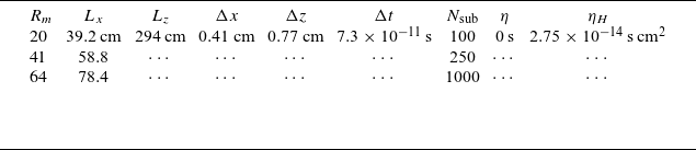
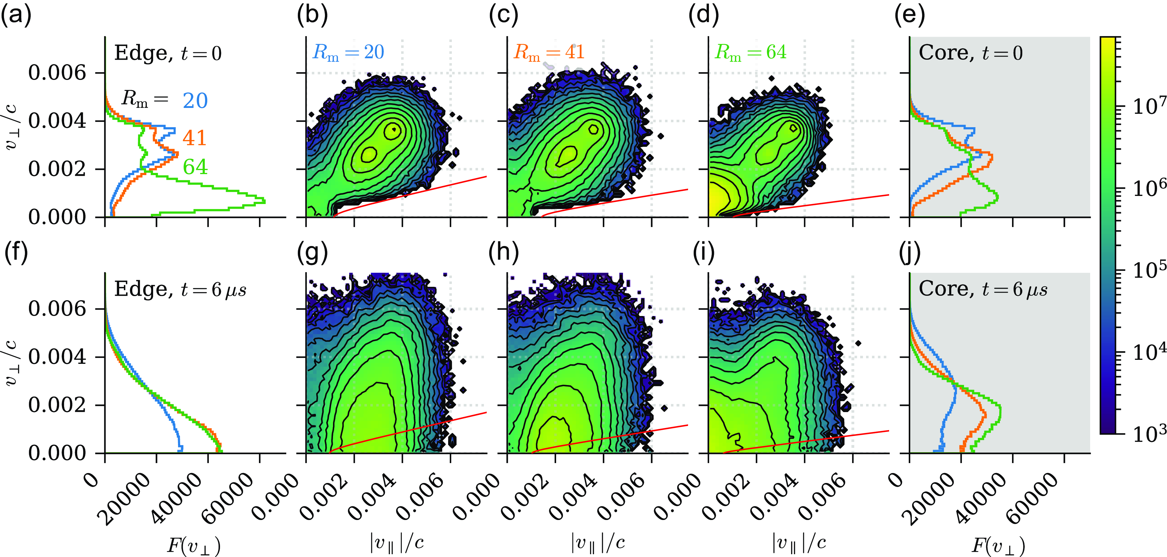
Figure 3. (a–e) Initial and (f–j) relaxed ion velocity distributions at the plasma edge, in three simulations. Edge ion distributions smooth and flatten in $v_\perp$
as the simulation evolves, with a stronger effect for edge plasma as compared with core plasma. The loss cone is filled, and the distribution varies little across the loss-cone boundary. (a) Reduced distribution
$v_\perp$
as the simulation evolves, with a stronger effect for edge plasma as compared with core plasma. The loss cone is filled, and the distribution varies little across the loss-cone boundary. (a) Reduced distribution $F(v_\perp )$
for simulations with vacuum
$F(v_\perp )$
for simulations with vacuum $R_{{m}} = 20$
(blue),
$R_{{m}} = 20$
(blue), $41$
(orange) and
$41$
(orange) and $64$
(green). Distribution is normalized so that
$64$
(green). Distribution is normalized so that $\int F(v_\perp ) 2\pi v_\perp \mathrm{d} v_\perp = 1$
. (b)–(d) The 2-D distributions
$\int F(v_\perp ) 2\pi v_\perp \mathrm{d} v_\perp = 1$
. (b)–(d) The 2-D distributions $f (v_\perp ,v_\parallel )$
for each of the three simulations shown in (a), normalized so that
$f (v_\perp ,v_\parallel )$
for each of the three simulations shown in (a), normalized so that $\int f 2\pi v_\perp \mathrm{d} v_\perp \mathrm{d} v_\parallel = 1$
. Red curves plot loss-cone boundary, with the effect of electrostatic trapping approximated using the on-axis potential well depth of
$\int f 2\pi v_\perp \mathrm{d} v_\perp \mathrm{d} v_\parallel = 1$
. Red curves plot loss-cone boundary, with the effect of electrostatic trapping approximated using the on-axis potential well depth of $0.4$
to
$0.4$
to $1.9 \;\mathrm{keV}$
. (e) Like (a), but a ‘core’ distribution centred on
$1.9 \;\mathrm{keV}$
. (e) Like (a), but a ‘core’ distribution centred on $r=0$
for comparison with the ‘edge’. (f)–(j) Like (a–e), but at later time
$r=0$
for comparison with the ‘edge’. (f)–(j) Like (a–e), but at later time $t=6\mu s$
in the simulation. In all panels, velocities
$t=6\mu s$
in the simulation. In all panels, velocities $v_\perp$
,
$v_\perp$
, $v_\parallel$
are normalized to the speed of light
$v_\parallel$
are normalized to the speed of light $c$
.
$c$
.
3. Results
3.1. Space, velocity structure of steady-state decay
At the start of each simulation, the plasma relaxes from its initial state over $\mathord {\sim } 1$
–
$\mathord {\sim } 1$
– $3 \tau _{\mathrm{bounce}}$
; the diamagnetic field response is changed, short-wavelength electrostatic fluctuations occur at the plasma edge and plasma escapes from the central cell into the expanders. The plasma reaches a steady-state decay by
$3 \tau _{\mathrm{bounce}}$
; the diamagnetic field response is changed, short-wavelength electrostatic fluctuations occur at the plasma edge and plasma escapes from the central cell into the expanders. The plasma reaches a steady-state decay by $t = 6 \tau _{\mathrm{bounce}}$
for all
$t = 6 \tau _{\mathrm{bounce}}$
for all $R_{{m}}$
simulations. At this time: (i) the particle loss time
$R_{{m}}$
simulations. At this time: (i) the particle loss time $\tau _{\mathrm{p}} = n / (\mathrm{d} n/\mathrm{d} t)$
is roughly constant and exceeds the ion bounce time (
$\tau _{\mathrm{p}} = n / (\mathrm{d} n/\mathrm{d} t)$
is roughly constant and exceeds the ion bounce time ( $\tau _{\mathrm{p}} \gg \tau _{\mathrm{bounce}}$
); (ii) the plasma beta
$\tau _{\mathrm{p}} \gg \tau _{\mathrm{bounce}}$
); (ii) the plasma beta $\beta _{{i}} = 8\pi P_{{i}}/B^2 \sim 0.1$
to within a factor of two at the origin
$\beta _{{i}} = 8\pi P_{{i}}/B^2 \sim 0.1$
to within a factor of two at the origin $(r,z) = (0,0)$
, with
$(r,z) = (0,0)$
, with $P_{{i}}$
the total ion pressure; (iii) the combined vacuum and diamagnetic fields attain a mirror ratio
$P_{{i}}$
the total ion pressure; (iii) the combined vacuum and diamagnetic fields attain a mirror ratio $R_{{m}} = \{ 21, 45, 69 \}$
somewhat higher than the respective vacuum values
$R_{{m}} = \{ 21, 45, 69 \}$
somewhat higher than the respective vacuum values $R_{{m}} = \{ 20, 41, 64 \}$
.
$R_{{m}} = \{ 20, 41, 64 \}$
.
Figure 1 shows the plasma’s overall structure at $t = 6 \tau _{\mathrm{bounce}}$
for each of the vacuum
$t = 6 \tau _{\mathrm{bounce}}$
for each of the vacuum $R_{{m}} = 20, 41, 64$
simulations. Flute-like, electrostatic fluctuations at the plasma’s radial edge are visible in
$R_{{m}} = 20, 41, 64$
simulations. Flute-like, electrostatic fluctuations at the plasma’s radial edge are visible in $z=0$
slices of ion density and electric fields, with the strongest and most coherent fluctuations for the
$z=0$
slices of ion density and electric fields, with the strongest and most coherent fluctuations for the $R_{{m}} = 20$
case. In figure 1(a,e,i), the axial outflow at
$R_{{m}} = 20$
case. In figure 1(a,e,i), the axial outflow at $|z| \gtrsim 70 \;\mathrm{cm}$
is split about
$|z| \gtrsim 70 \;\mathrm{cm}$
is split about $r = 0$
, so more plasma escapes from the radial edge
$r = 0$
, so more plasma escapes from the radial edge $r \gt 0$
than the core
$r \gt 0$
than the core $r \sim 0$
. In figure 1(d,h,l), the radial electric field fluctuation
$r \sim 0$
. In figure 1(d,h,l), the radial electric field fluctuation $\delta E_r = E_r - \langle E_r \rangle _\theta$
, where
$\delta E_r = E_r - \langle E_r \rangle _\theta$
, where $\langle \cdots \rangle _\theta$
represents an average over the azimuthal coordinate to subtract the plasma’s net radial potential. The azimuthal fluctuation
$\langle \cdots \rangle _\theta$
represents an average over the azimuthal coordinate to subtract the plasma’s net radial potential. The azimuthal fluctuation $\delta E_\theta$
in figure 1(c,g,k) is defined similarly. The transverse magnetic fluctuations
$\delta E_\theta$
in figure 1(c,g,k) is defined similarly. The transverse magnetic fluctuations $\delta B_r$
and
$\delta B_r$
and $\delta B_\theta$
have small amplitudes
$\delta B_\theta$
have small amplitudes $\lesssim 10^{-3} B(z=0)$
, whereas the electric fluctuations
$\lesssim 10^{-3} B(z=0)$
, whereas the electric fluctuations $\delta E_r$
and
$\delta E_r$
and $\delta E_\theta$
are of order
$\delta E_\theta$
are of order $0.1 v_{\mathrm{ti0}} B(z=0)/c$
, corresponding to motional flows at thermal speeds. We therefore neglect electromagnetic fluctuations and focus solely on the azimuthal, electrostatic mode visible in figure 1.
$0.1 v_{\mathrm{ti0}} B(z=0)/c$
, corresponding to motional flows at thermal speeds. We therefore neglect electromagnetic fluctuations and focus solely on the azimuthal, electrostatic mode visible in figure 1.
Figure 2(a,b) shows ion density profiles along $z$
both on- and off-axis, with horizontal dashes marking the density floor imposed in Ohm’s law, (2.1). The off-axis density is measured along flux surfaces hosting the strong electric fluctuations seen in figure 1. Specifically, we pick surfaces at
$z$
both on- and off-axis, with horizontal dashes marking the density floor imposed in Ohm’s law, (2.1). The off-axis density is measured along flux surfaces hosting the strong electric fluctuations seen in figure 1. Specifically, we pick surfaces at $r=\{9,18,22\}\;\mathrm{cm}$
and
$r=\{9,18,22\}\;\mathrm{cm}$
and $z=0$
that have an approximate (azimuth-averaged, paraxial) flux coordinate
$z=0$
that have an approximate (azimuth-averaged, paraxial) flux coordinate $\psi \approx \int 2\pi \langle B_z \rangle _\theta r \mathrm{d} r = \{ 2.1, 3.8, 3.7\} \times 10^6 \;\mathrm{G\,cm^{2}}$
for the
$\psi \approx \int 2\pi \langle B_z \rangle _\theta r \mathrm{d} r = \{ 2.1, 3.8, 3.7\} \times 10^6 \;\mathrm{G\,cm^{2}}$
for the $R_{{m}}=\{20,41,64\}$
simulations, respectively. The plotted density
$R_{{m}}=\{20,41,64\}$
simulations, respectively. The plotted density $n_{{i}}$
is also azimuth averaged.
$n_{{i}}$
is also azimuth averaged.
The density profiles peak near the turning points of $45^\circ$
pitch-angle ions, defined as the
$45^\circ$
pitch-angle ions, defined as the $z$
locations where the local mirror ratio
$z$
locations where the local mirror ratio $R_{{m}}(z)=2$
on axis; i.e.
$R_{{m}}(z)=2$
on axis; i.e. $\{57,44,36\} \;\mathrm{cm}$
(figure 2
c). Comparing on- and off-axis density peaks, the off-axis peak is wider and decreases more slowly towards the mirror throat and expander. This can be explained by the plasma edge’s stronger loss-cone outflow and broader pitch-angle distribution between
$\{57,44,36\} \;\mathrm{cm}$
(figure 2
c). Comparing on- and off-axis density peaks, the off-axis peak is wider and decreases more slowly towards the mirror throat and expander. This can be explained by the plasma edge’s stronger loss-cone outflow and broader pitch-angle distribution between $0^\circ$
and
$0^\circ$
and $45^\circ$
, compared with the plasma core at
$45^\circ$
, compared with the plasma core at $r = 0$
(figure 3).
$r = 0$
(figure 3).
Figure 2(d) shows on- and off-axis electrostatic potential profiles $e\phi (z)/T_{{e}}$
. The off-axis profiles
$e\phi (z)/T_{{e}}$
. The off-axis profiles $\phi (s(z)) = -\int E_\parallel (s) \mathrm{d} s$
, with arclength
$\phi (s(z)) = -\int E_\parallel (s) \mathrm{d} s$
, with arclength $s$
in the
$s$
in the $(r,z)$
plane, are integrated along the same flux surfaces used in figure 2(b). We notice that the
$(r,z)$
plane, are integrated along the same flux surfaces used in figure 2(b). We notice that the $z=0$
potential well has similar depth both on- and off-axis. The density floor truncates the axial electrostatic potential at
$z=0$
potential well has similar depth both on- and off-axis. The density floor truncates the axial electrostatic potential at $z \approx 100$
to
$z \approx 100$
to $110 \;\mathrm{cm}$
, so the full potential drop from the mirror throat to the domain’s
$110 \;\mathrm{cm}$
, so the full potential drop from the mirror throat to the domain’s $z$
boundary is not captured in our simulation. In any case, plasma outflow in the expanders is not well modelled by our electron closure, as the outflow is far from thermal equilibrium (e.g. Wetherton et al. Reference Wetherton, Le, Egedal, Forest, Daughton, Stanier and Boldyrev2021). We will restrict our attention to central-cell plasma behaviour that we suppose to be unaffected by the expanders.
$z$
boundary is not captured in our simulation. In any case, plasma outflow in the expanders is not well modelled by our electron closure, as the outflow is far from thermal equilibrium (e.g. Wetherton et al. Reference Wetherton, Le, Egedal, Forest, Daughton, Stanier and Boldyrev2021). We will restrict our attention to central-cell plasma behaviour that we suppose to be unaffected by the expanders.
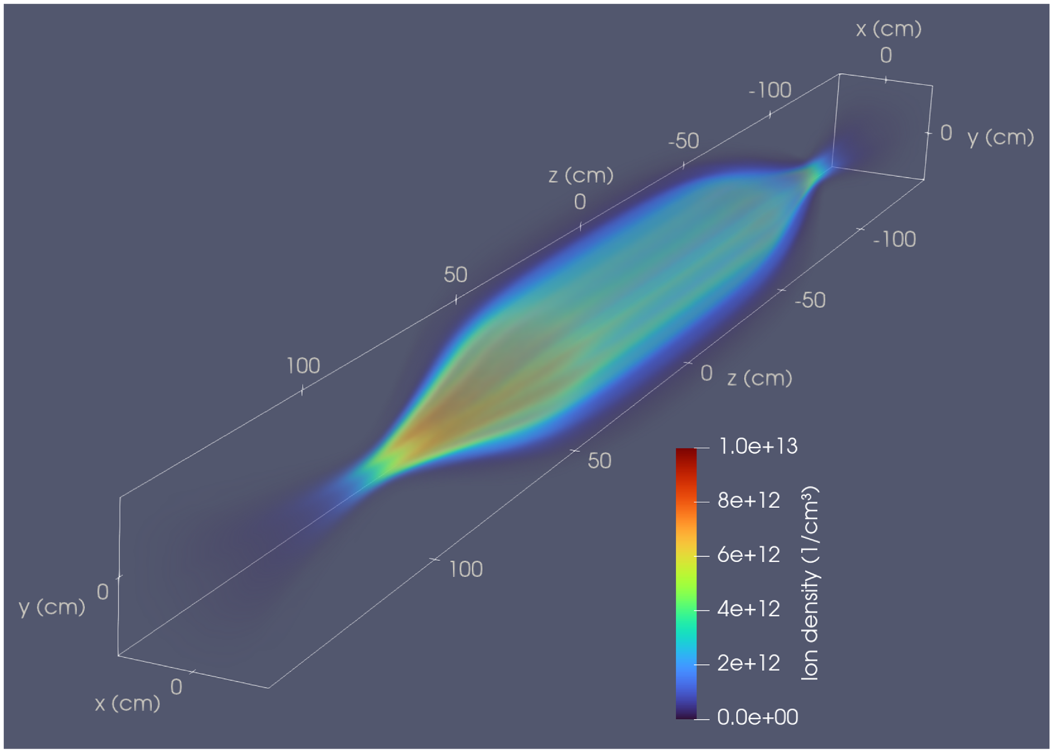
Figure 4. The 3-D rendering of ion density in $R_{{m}}=20$
simulation at
$R_{{m}}=20$
simulation at $t=6\;\mathrm{\unicode{x03BC}s}$
; colourmap is ion density in units of
$t=6\;\mathrm{\unicode{x03BC}s}$
; colourmap is ion density in units of $\mathrm{cm}^{-3}$
. An animated movie is available in the online journal.
$\mathrm{cm}^{-3}$
. An animated movie is available in the online journal.
Figure 3 shows initial ion velocity distributions, as imported into Hybrid-VPIC from CQL3D-m, at the centre of the mirror cell: $z \in (-5.9, 5.9) \;\mathrm{cm}$
for all simulations. Figure 3(a–d) sample ions from the plasma’s radial edge:
$z \in (-5.9, 5.9) \;\mathrm{cm}$
for all simulations. Figure 3(a–d) sample ions from the plasma’s radial edge: $r \in [ 5.9, 11.8) \;\mathrm{cm}$
for
$r \in [ 5.9, 11.8) \;\mathrm{cm}$
for $R_{{m}} = 20$
;
$R_{{m}} = 20$
; $r \in [11.8, 23.5) \;\mathrm{cm}$
for
$r \in [11.8, 23.5) \;\mathrm{cm}$
for $R_{{m}} = 41$
;
$R_{{m}} = 41$
; $r \in [14.7, 29.4) \;\mathrm{cm}$
for
$r \in [14.7, 29.4) \;\mathrm{cm}$
for $R_{{m}} = 64$
. Figure 3(e) samples ions from the plasma’s core:
$R_{{m}} = 64$
. Figure 3(e) samples ions from the plasma’s core: $r \in [0,2.9) \;\mathrm{cm}$
for
$r \in [0,2.9) \;\mathrm{cm}$
for $R_{{m}} = 20$
;
$R_{{m}} = 20$
; $r \in [0,5.9) \;\mathrm{cm}$
for
$r \in [0,5.9) \;\mathrm{cm}$
for $R_{{m}} = 41$
;
$R_{{m}} = 41$
; $r \in [0,7.4) \;\mathrm{cm}$
for
$r \in [0,7.4) \;\mathrm{cm}$
for $R_{{m}} = 64$
. Figure 3(f–j) shows ion distributions, selected from the same axial and radial regions as figure 3(a–e), after the simulation has reached
$R_{{m}} = 64$
. Figure 3(f–j) shows ion distributions, selected from the same axial and radial regions as figure 3(a–e), after the simulation has reached $t = 6 \tau _{\mathrm{bounce}} \approx 6 \;\mathrm{\unicode{x03BC}s}$
. Ions diffuse mostly in
$t = 6 \tau _{\mathrm{bounce}} \approx 6 \;\mathrm{\unicode{x03BC}s}$
. Ions diffuse mostly in $v_\perp$
; their distribution is continuous and nearly flat across the velocity-space loss-cone boundary. The reduced distribution
$v_\perp$
; their distribution is continuous and nearly flat across the velocity-space loss-cone boundary. The reduced distribution $F(v_\perp ) = \int f \mathrm{d} v_\parallel$
has relaxed to a monotonically decreasing shape,
$F(v_\perp ) = \int f \mathrm{d} v_\parallel$
has relaxed to a monotonically decreasing shape, $\mathrm{d} F / \mathrm{d} v_\perp \lt 0$
, at the plasma edge (figure 3
f); however, the core plasma maintains
$\mathrm{d} F / \mathrm{d} v_\perp \lt 0$
, at the plasma edge (figure 3
f); however, the core plasma maintains $\mathrm{d} F / \mathrm{d} v_\perp \gt 0$
at low
$\mathrm{d} F / \mathrm{d} v_\perp \gt 0$
at low $v_\perp$
(figure 3
j). Some distribution function moments will be used in later discussion. We define
$v_\perp$
(figure 3
j). Some distribution function moments will be used in later discussion. We define $\boldsymbol{B}$
-perpendicular and parallel temperatures
$\boldsymbol{B}$
-perpendicular and parallel temperatures $T_{\mathrm{i\perp }} \equiv (1/2) \int m_{{i}} v_\perp ^2 f \mathrm{d}\boldsymbol{v}$
and
$T_{\mathrm{i\perp }} \equiv (1/2) \int m_{{i}} v_\perp ^2 f \mathrm{d}\boldsymbol{v}$
and $T_{\mathrm{i\parallel }} \equiv \int m_{{i}} v_\parallel ^2 f \mathrm{d}\boldsymbol{v}$
so that
$T_{\mathrm{i\parallel }} \equiv \int m_{{i}} v_\parallel ^2 f \mathrm{d}\boldsymbol{v}$
so that $T_{{i}} = (2T_{\mathrm{i\perp }} + T_{\mathrm{i\parallel }})/3$
; temperature values for the edge ion distributions at
$T_{{i}} = (2T_{\mathrm{i\perp }} + T_{\mathrm{i\parallel }})/3$
; temperature values for the edge ion distributions at $t=6\,\tau _{\mathrm{bounce}}$
(figure 3
f–i) are given in table 1.
$t=6\,\tau _{\mathrm{bounce}}$
(figure 3
f–i) are given in table 1.
Figure 4 shows a 3-D render of ion density in the $R_{{m}}=20$
simulation at
$R_{{m}}=20$
simulation at $t=6\;\mathrm{\unicode{x03BC}s}$
. The flute-like (
$t=6\;\mathrm{\unicode{x03BC}s}$
. The flute-like ( $k_\parallel \sim 0$
) nature of the edge fluctuations is apparent. An accompanying movie of the full time evolution from
$k_\parallel \sim 0$
) nature of the edge fluctuations is apparent. An accompanying movie of the full time evolution from $t=0$
to
$t=0$
to $6\;\mathrm{\unicode{x03BC}s}$
is available in the online journal.
$6\;\mathrm{\unicode{x03BC}s}$
is available in the online journal.
To summarize, figures 1–4 show that at the plasma’s radial edge: (i) flute-like electrostatic fluctuations appear; (ii) axial outflow and hence losses are enhanced relative to the plasma’s core at $r \sim 0$
; and (iii) ions diffuse in
$r \sim 0$
; and (iii) ions diffuse in $v_\perp$
to drive
$v_\perp$
to drive $\mathrm{d} F/\mathrm{d} v_\perp \lt 0$
. It is already natural to suspect that the electrostatic fluctuations diffuse ions into the loss cone and hence cause plasma to escape the mirror.
$\mathrm{d} F/\mathrm{d} v_\perp \lt 0$
. It is already natural to suspect that the electrostatic fluctuations diffuse ions into the loss cone and hence cause plasma to escape the mirror.

Figure 5. Radial structure of plasma at midplane $z=0$
and at
$z=0$
and at $t = 6 \,\tau _{\mathrm{bounce}} \approx 6 \;\mathrm{\unicode{x03BC}s}$
, for simulations with vacuum (a–e)
$t = 6 \,\tau _{\mathrm{bounce}} \approx 6 \;\mathrm{\unicode{x03BC}s}$
, for simulations with vacuum (a–e) $R_{{m}}=20$
, (f–j)
$R_{{m}}=20$
, (f–j) $41$
, (k–o)
$41$
, (k–o) $64$
. Panels (a–c), (f–h) and (k–l) show azimuth-averaged radial profiles of (a) ion density
$64$
. Panels (a–c), (f–h) and (k–l) show azimuth-averaged radial profiles of (a) ion density $n_{{i}}$
, (b) ion density gradient
$n_{{i}}$
, (b) ion density gradient $\epsilon \rho _{\mathrm{i0}}$
, (c) azimuthal electrostatic fluctuation energy
$\epsilon \rho _{\mathrm{i0}}$
, (c) azimuthal electrostatic fluctuation energy $\delta E_\theta ^2$
. Horizontal shaded bars contain the ‘edge’ ion distributions from figure 3. Vertical dashes in (a), (f) and (k) mark density floor for (2.1). Panels (d), (e), (i), (j), and (n), (o) show azimuthal Fourier spectra of density
$\delta E_\theta ^2$
. Horizontal shaded bars contain the ‘edge’ ion distributions from figure 3. Vertical dashes in (a), (f) and (k) mark density floor for (2.1). Panels (d), (e), (i), (j), and (n), (o) show azimuthal Fourier spectra of density $\tilde {n}_{{i}}(r,m)$
and azimuthal electric field
$\tilde {n}_{{i}}(r,m)$
and azimuthal electric field $\tilde {E}_\theta (r,m)$
; Fourier transform maps
$\tilde {E}_\theta (r,m)$
; Fourier transform maps $\theta \to m$
, but radius
$\theta \to m$
, but radius $r$
is not transformed. White rays mark azimuthal wavenumber
$r$
is not transformed. White rays mark azimuthal wavenumber $k \rho _{\mathrm{i0}} = 2,4,6,8,10,12$
, with
$k \rho _{\mathrm{i0}} = 2,4,6,8,10,12$
, with $k = m/r$
. Dashed pink ray is the maximum
$k = m/r$
. Dashed pink ray is the maximum $k = \pi /\Delta r$
resolved by the spatial grid, taking
$k = \pi /\Delta r$
resolved by the spatial grid, taking $\Delta r = \sqrt {2} \Delta x$
. Panels (f)–(j) and (k)–(o) are organized similarly.
$\Delta r = \sqrt {2} \Delta x$
. Panels (f)–(j) and (k)–(o) are organized similarly.
3.2. Drift cyclotron mode identification
To establish the electrostatic mode’s nature, we need to know plasma properties at the radial edge and the mode’s wavenumber and frequency spectrum.
Figure 5(a–c,f–h,k–l) presents the radial structure of the ion density $n_{{i}}$
, and the electrostatic fluctuation energy
$n_{{i}}$
, and the electrostatic fluctuation energy $\delta E_\theta ^2 = \langle E_\theta ^2 \rangle _\theta - \langle E_\theta \rangle _\theta ^2$
, at the mirror midplane
$\delta E_\theta ^2 = \langle E_\theta ^2 \rangle _\theta - \langle E_\theta \rangle _\theta ^2$
, at the mirror midplane $z=0$
. Figure 5(d,e,i,j,n,o) also presents Fourier spectra of density
$z=0$
. Figure 5(d,e,i,j,n,o) also presents Fourier spectra of density $\tilde {n}_{{i}}(m,r)$
and electric component
$\tilde {n}_{{i}}(m,r)$
and electric component $\tilde {E}_\theta (m,r)$
as a function of azimuthal mode number
$\tilde {E}_\theta (m,r)$
as a function of azimuthal mode number $m$
and radius
$m$
and radius $r$
. Beware that Fourier spectrum normalization is arbitrary here and in all figures; Fourier amplitudes may be compared between panels within one figure, but not across distinct figures.
$r$
. Beware that Fourier spectrum normalization is arbitrary here and in all figures; Fourier amplitudes may be compared between panels within one figure, but not across distinct figures.
The density gradient $\epsilon \equiv (\mathrm{d} n_{{i}}/\mathrm{d} r)/n_{{i}}$
, in units of inverse ion Larmor radius
$\epsilon \equiv (\mathrm{d} n_{{i}}/\mathrm{d} r)/n_{{i}}$
, in units of inverse ion Larmor radius $\rho _{\mathrm{i0}}^{-1}$
, is of order unity and increases with
$\rho _{\mathrm{i0}}^{-1}$
, is of order unity and increases with $R_{{m}}$
(figure 5
b,g,l); equivalently, the plasma column radius is smaller in units of
$R_{{m}}$
(figure 5
b,g,l); equivalently, the plasma column radius is smaller in units of $\rho _{\mathrm{i0}}$
for larger
$\rho _{\mathrm{i0}}$
for larger $R_{{m}}$
, despite the column’s larger physical extent.
$R_{{m}}$
, despite the column’s larger physical extent.
The mode spectra of $\tilde {n}$
and
$\tilde {n}$
and $\tilde {E}_\theta$
suggest a partial decoupling of density and electric fluctuations (figure 5, d, e, i, j, n, o). In all simulations, low
$\tilde {E}_\theta$
suggest a partial decoupling of density and electric fluctuations (figure 5, d, e, i, j, n, o). In all simulations, low $m \sim 2$
–
$m \sim 2$
– $4$
density fluctuations are not accompanied by a strong
$4$
density fluctuations are not accompanied by a strong $E_\theta$
signal (figure 5
d, e, i, j, n, o). The
$E_\theta$
signal (figure 5
d, e, i, j, n, o). The $R_{{m}}=20$
simulation shows a strong mode in both density and
$R_{{m}}=20$
simulation shows a strong mode in both density and $E_\theta$
fluctuations at
$E_\theta$
fluctuations at $m \approx 9$
–
$m \approx 9$
– $10$
and equivalent angular wavenumber
$10$
and equivalent angular wavenumber $k \rho _{\mathrm{i0}} \approx 2$
–
$k \rho _{\mathrm{i0}} \approx 2$
– $4$
(figure 5
d,e). We identify this Fourier signal with phase-coherent fluting at the same
$4$
(figure 5
d,e). We identify this Fourier signal with phase-coherent fluting at the same $m$
visible to the eye in figure 1(b,c). In contrast, the
$m$
visible to the eye in figure 1(b,c). In contrast, the $R_{{m}}=41,64$
simulations show a decoupling of density and
$R_{{m}}=41,64$
simulations show a decoupling of density and $E_\theta$
fluctuations. The strongest density fluctuations reside at
$E_\theta$
fluctuations. The strongest density fluctuations reside at $r \sim 1$
–
$r \sim 1$
– $2\rho _{\mathrm{i0}}$
,
$2\rho _{\mathrm{i0}}$
, $m \sim 7$
–
$m \sim 7$
– $8$
and
$8$
and $k\rho _{\mathrm{i0}} \approx 2$
–
$k\rho _{\mathrm{i0}} \approx 2$
– $6$
(figure 5
i,n), whereas the electrostatic fluctuations reside at larger
$6$
(figure 5
i,n), whereas the electrostatic fluctuations reside at larger $r \sim 2$
–
$r \sim 2$
– $4\rho _{\mathrm{i0}}$
,
$4\rho _{\mathrm{i0}}$
, $m \sim 15$
–
$m \sim 15$
– $30$
and
$30$
and $k \rho _{\mathrm{i0}} \sim 4$
–
$k \rho _{\mathrm{i0}} \sim 4$
– $12$
(figure 5
j,o).
$12$
(figure 5
j,o).
The fluctuations have $k_\parallel \ll k_\perp$
and are thus flute-like, which we checked by plotting
$k_\parallel \ll k_\perp$
and are thus flute-like, which we checked by plotting $\boldsymbol{E}$
in approximate flux-surface coordinates (not shown). Electric-field fluctuations terminate at the mirror throats and do not extend into the expanders; fluctuations may be artificially truncated by the density floor in (2.1).
$\boldsymbol{E}$
in approximate flux-surface coordinates (not shown). Electric-field fluctuations terminate at the mirror throats and do not extend into the expanders; fluctuations may be artificially truncated by the density floor in (2.1).
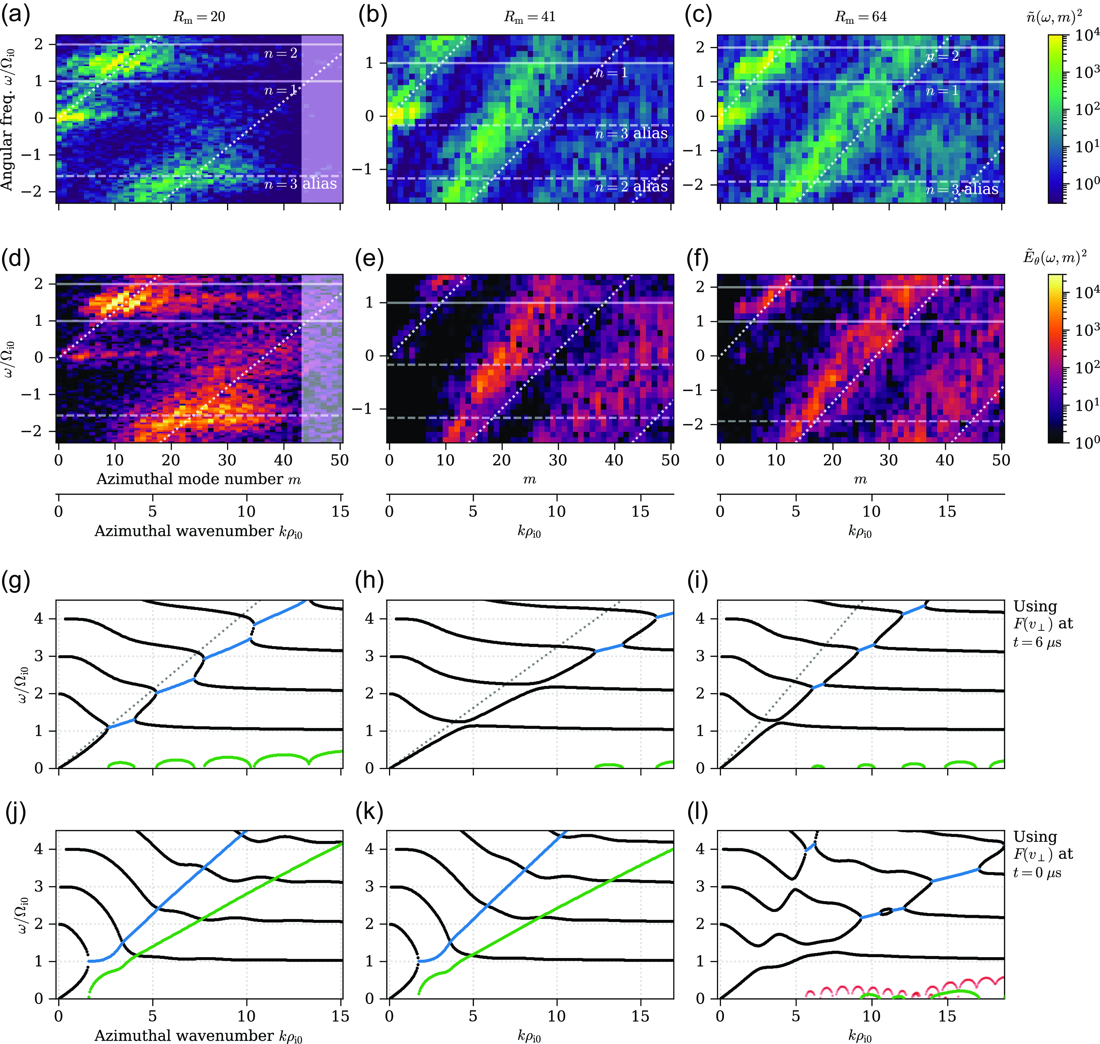
Figure 6. Time-azimuth Fourier spectra of density $\tilde {n}(\omega ,m)^2$
(a–c) and electric field
$\tilde {n}(\omega ,m)^2$
(a–c) and electric field $\tilde {E}_\theta (\omega ,m)^2$
(d–f) for simulations with
$\tilde {E}_\theta (\omega ,m)^2$
(d–f) for simulations with $R_{{m}}=\{20, 41, 64\}$
(left to right). Panels (g)–(l) show corresponding
$R_{{m}}=\{20, 41, 64\}$
(left to right). Panels (g)–(l) show corresponding $(\omega ,k)$
of unstable DCLC modes predicted by (3.4) for edge
$(\omega ,k)$
of unstable DCLC modes predicted by (3.4) for edge $F(v_\perp )$
at
$F(v_\perp )$
at $t \approx 6 \;\mathrm{\unicode{x03BC}s}$
(g–i) or
$t \approx 6 \;\mathrm{\unicode{x03BC}s}$
(g–i) or $t = 0$
(j–l). In panels (a)–(f), the full
$t = 0$
(j–l). In panels (a)–(f), the full $\omega$
range within Nyquist-sampling limits is shown; signals with
$\omega$
range within Nyquist-sampling limits is shown; signals with $\omega \gtrsim 2 \Omega _{\mathrm{i0}}$
alias in frequency. White dotted lines plot ion diamagnetic drift velocity
$\omega \gtrsim 2 \Omega _{\mathrm{i0}}$
alias in frequency. White dotted lines plot ion diamagnetic drift velocity $\omega /k = v_{\mathrm{Di}}$
. Shaded vertical bar in (a), (d) marks grid resolution limit
$\omega /k = v_{\mathrm{Di}}$
. Shaded vertical bar in (a), (d) marks grid resolution limit $k \gt \pi /\Delta r$
with
$k \gt \pi /\Delta r$
with $\Delta r = \sqrt {2}\Delta x$
. In (g)–(l), we plot both stable- and unstable-mode frequencies
$\Delta r = \sqrt {2}\Delta x$
. In (g)–(l), we plot both stable- and unstable-mode frequencies $\textrm {Re}(\omega )$
(black, blue), and also the corresponding unstable-mode growth rates
$\textrm {Re}(\omega )$
(black, blue), and also the corresponding unstable-mode growth rates $\textrm {Im}(\omega )$
(green). In (l) only, red curves plot
$\textrm {Im}(\omega )$
(green). In (l) only, red curves plot $\textrm {Im}(\omega )$
for higher-
$\textrm {Im}(\omega )$
for higher- $\omega /k$
modes with
$\omega /k$
modes with $\textrm {Re}(\omega ) \in [4\Omega _{\mathrm{i0}},14\Omega _{\mathrm{i0}}]$
beyond the plot extent. Black dotted lines plot
$\textrm {Re}(\omega ) \in [4\Omega _{\mathrm{i0}},14\Omega _{\mathrm{i0}}]$
beyond the plot extent. Black dotted lines plot $\omega /k = v_{\mathrm{Di}}$
.
$\omega /k = v_{\mathrm{Di}}$
.
Joint time-frequency and azimuthal-mode spectra of density and electric field fluctuations, $\tilde {n}(\omega ,m)$
and
$\tilde {n}(\omega ,m)$
and $\tilde {E}_\theta (\omega ,m)$
, are presented in figure 6(a–f). Fluctuations are sampled at radii
$\tilde {E}_\theta (\omega ,m)$
, are presented in figure 6(a–f). Fluctuations are sampled at radii $r = \{3.34, 2.98, 2.69 \} \rho _{\mathrm{i0}}$
, respectively, over
$r = \{3.34, 2.98, 2.69 \} \rho _{\mathrm{i0}}$
, respectively, over $t = 3$
to
$t = 3$
to $6 \,\tau _{\mathrm{bounce}}$
;
$6 \,\tau _{\mathrm{bounce}}$
; $\omega$
is angular frequency. Positive
$\omega$
is angular frequency. Positive $\omega /k$
corresponds to the ion diamagnetic drift direction. We interpret Fourier power at
$\omega /k$
corresponds to the ion diamagnetic drift direction. We interpret Fourier power at $\omega \lt 0$
as high-
$\omega \lt 0$
as high- $\omega$
signal that is aliased in frequency space and would otherwise be contiguous in physical
$\omega$
signal that is aliased in frequency space and would otherwise be contiguous in physical $(\omega ,k)$
. Assuming so, both
$(\omega ,k)$
. Assuming so, both $\tilde {n}$
and
$\tilde {n}$
and $\tilde {E}_\theta$
show a mode spectrum with a phase speed
$\tilde {E}_\theta$
show a mode spectrum with a phase speed $\omega /k \gt 0$
comparable to the ion diamagnetic drift speed
$\omega /k \gt 0$
comparable to the ion diamagnetic drift speed $v_{\mathrm{Di}}$
(white dotted lines, figure 6
a–f). We compute
$v_{\mathrm{Di}}$
(white dotted lines, figure 6
a–f). We compute
 \begin{equation} v_{\mathrm{Di}} \approx \frac {T_{\mathrm{i\perp }}/m_{{i}}}{\Omega _{\mathrm{i0}}} \left (-\frac {1}{n_{{i}}} \frac {\mathrm{d} n_{{i}}}{\mathrm{d} r}\right ) = v_{\mathrm{ti0}} \frac {T_{\mathrm{i\perp }}}{T_{\mathrm{i0}}} |\epsilon | \rho _{\mathrm{i0}} \end{equation}
using $\epsilon \rho _{\mathrm{i0}} = \{ -1, -1, -1.5 \}$
and
$\epsilon \rho _{\mathrm{i0}} = \{ -1, -1, -1.5 \}$
and $T_{\mathrm{i\perp }}$
measured at
$T_{\mathrm{i\perp }}$
measured at $t=6\tau _{\mathrm{bounce}}$
(values reported in § 3.1). The spectra align with
$t=6\tau _{\mathrm{bounce}}$
(values reported in § 3.1). The spectra align with $\omega /k = v_{\mathrm{Di}}$
within a factor of
$\omega /k = v_{\mathrm{Di}}$
within a factor of $2$
.
$2$
.
A fundamental mode appears at $\omega \in [\Omega _{\mathrm{i0}}, 2 \Omega _{\mathrm{i0}}]$
in all simulations. Fluctuation power extends to
$\omega \in [\Omega _{\mathrm{i0}}, 2 \Omega _{\mathrm{i0}}]$
in all simulations. Fluctuation power extends to $\omega \gtrsim 3 \Omega _{\mathrm{i0}}$
in all simulations, perhaps up to
$\omega \gtrsim 3 \Omega _{\mathrm{i0}}$
in all simulations, perhaps up to $\omega \gtrsim 7 \Omega _{\mathrm{i0}}$
in the
$\omega \gtrsim 7 \Omega _{\mathrm{i0}}$
in the $R_{{m}}=64$
simulation, but by eye we do not discern discrete harmonics above
$R_{{m}}=64$
simulation, but by eye we do not discern discrete harmonics above $2 \Omega _{\mathrm{i0}}$
. A low-frequency
$2 \Omega _{\mathrm{i0}}$
. A low-frequency $\omega \ll \Omega _{\mathrm{i0}}$
mode with non-zero
$\omega \ll \Omega _{\mathrm{i0}}$
mode with non-zero $m$
appears chiefly in
$m$
appears chiefly in $\tilde {n}$
and weakly in
$\tilde {n}$
and weakly in $\tilde {E}_\theta$
; we identify this slower motion as fluid interchange and discuss it further in § 4.4.
$\tilde {E}_\theta$
; we identify this slower motion as fluid interchange and discuss it further in § 4.4.
To help interpret figure 6(a–f), we compute the linearly unstable $(\omega ,k)$
for DCLC in a planar-slab plasma with a spatial density gradient
$(\omega ,k)$
for DCLC in a planar-slab plasma with a spatial density gradient $\epsilon$
and uniform background magnetic field (
$\epsilon$
and uniform background magnetic field ( ${\nabla } B = 0$
). In such a plasma, a dispersion relation for exactly perpendicular electrostatic waves can be obtained by integrating over unperturbed orbits and Taylor expanding
${\nabla } B = 0$
). In such a plasma, a dispersion relation for exactly perpendicular electrostatic waves can be obtained by integrating over unperturbed orbits and Taylor expanding $f$
in particle guiding-centre coordinate, following Stix (Reference Stix1992, § 14–3, (9)). The dispersion relation is then
$f$
in particle guiding-centre coordinate, following Stix (Reference Stix1992, § 14–3, (9)). The dispersion relation is then
 \begin{equation} D = 1 + \sum _s \chi _s = 0,\end{equation}
where the perpendicular ( $k=k_\perp$
) susceptibility of species
$k=k_\perp$
) susceptibility of species $s$
reads
$s$
reads
 \begin{align} \chi _{\mathrm{s}} = \left (\frac {\omega _{\mathrm{p}s}}{\Omega _{\mathrm{s}}}\right )^2 \bigg [ \left ( 1 - \frac {\epsilon \omega }{k} \right ) \frac {1}{k^2} &\sum _{n=-\infty }^{\infty } \frac {n}{\omega - n} \int \mathrm{d}^3\boldsymbol{v} \left ( \frac {1}{v_\perp } \frac {\partial f}{\partial v_\perp } \right ) J_n^2 \nonumber \\ - \frac {\epsilon }{k} &\sum _{n=-\infty }^{\infty } \frac {1}{\omega - n} \int \mathrm{d}^3\boldsymbol{v} f J_n^2 \bigg ] . \end{align}
In (3.3), variables are written in a species-specific dimensionless form: $\omega /\Omega _{\mathrm{s}} \to \omega$
,
$\omega /\Omega _{\mathrm{s}} \to \omega$
, $k\rho _s \to k$
,
$k\rho _s \to k$
, $\epsilon \rho _s \to \epsilon$
and
$\epsilon \rho _s \to \epsilon$
and $v_\perp /v_{\mathrm{t}s} \to v_\perp$
, where
$v_\perp /v_{\mathrm{t}s} \to v_\perp$
, where $\Omega _{\mathrm{s}}$
is signed (i.e.
$\Omega _{\mathrm{s}}$
is signed (i.e. $\Omega _{{e}} \lt 0$
) and
$\Omega _{{e}} \lt 0$
) and $\rho _s \equiv v_{\mathrm{t}s}/\Omega _{\mathrm{s}}$
. The decision of how to define
$\rho _s \equiv v_{\mathrm{t}s}/\Omega _{\mathrm{s}}$
. The decision of how to define $v_{\mathrm{t}s}$
(with or without
$v_{\mathrm{t}s}$
(with or without $\sqrt {2}$
) is given to the user. The plasma frequency
$\sqrt {2}$
) is given to the user. The plasma frequency $\omega _{\mathrm{p}s} = \sqrt {4\pi n_{\mathrm{s}} q_{\mathrm{s}}^2/m_{\mathrm{s}}}$
for each species. The Bessel functions
$\omega _{\mathrm{p}s} = \sqrt {4\pi n_{\mathrm{s}} q_{\mathrm{s}}^2/m_{\mathrm{s}}}$
for each species. The Bessel functions $J_n = J_n(k_\perp v_\perp )$
as usual, with
$J_n = J_n(k_\perp v_\perp )$
as usual, with $k_\perp =k$
. Equations (3.2)–(3.3) simplify for cold fluid electrons to yield
$k_\perp =k$
. Equations (3.2)–(3.3) simplify for cold fluid electrons to yield
 \begin{equation} D = 1 + \chi _{{i}} + \frac {\omega _{\mathrm{pe}}^2}{\Omega _{{e}}^2} + \frac {\omega _{\mathrm{pe}}^2}{|\Omega _{{e}}|} \frac {\epsilon }{k \omega } = 0 , \end{equation}
where the variables $k$
,
$k$
, $\epsilon$
and
$\epsilon$
and $\omega$
are now in dimensional units. Equation (3.4) is the slab DCLC dispersion relation also used by Lindgren et al. (Reference Lindgren, Birdsall and Langdon1976, (2)), Ferraro et al. (Reference Ferraro, Littlejohn, Sanuki and Fried1987, (19)), and Kotelnikov et al. (Reference Kotelnikov, Chernoshtanov and Prikhodko2017, (17) and (A14)). In our sign convention,
$\omega$
are now in dimensional units. Equation (3.4) is the slab DCLC dispersion relation also used by Lindgren et al. (Reference Lindgren, Birdsall and Langdon1976, (2)), Ferraro et al. (Reference Ferraro, Littlejohn, Sanuki and Fried1987, (19)), and Kotelnikov et al. (Reference Kotelnikov, Chernoshtanov and Prikhodko2017, (17) and (A14)). In our sign convention, $\epsilon \lt 0$
obtains DCLC with
$\epsilon \lt 0$
obtains DCLC with $\omega /k \gt 0$
in the ion diamagnetic drift direction. Equation (3.4) also hosts normal modes with
$\omega /k \gt 0$
in the ion diamagnetic drift direction. Equation (3.4) also hosts normal modes with $k \lt 0$
and high phase velocity in the electron diamagnetic drift direction (Lindgren et al. Reference Lindgren, Birdsall and Langdon1976, § 2.A.1.b), which do not appear in our simulations and so are omitted from our discussion.
$k \lt 0$
and high phase velocity in the electron diamagnetic drift direction (Lindgren et al. Reference Lindgren, Birdsall and Langdon1976, § 2.A.1.b), which do not appear in our simulations and so are omitted from our discussion.
The unstable- and normal-mode solutions to (3.4), presented in figure 6(g–l), are computed as follows. First, we take $\Omega _{\mathrm{i0}}$
,
$\Omega _{\mathrm{i0}}$
, $\rho _{\mathrm{i0}}$
and
$\rho _{\mathrm{i0}}$
and $v_{\mathrm{ti0}}$
as defined in § 2.3 to normalize all variables in (3.4). Plasma parameters used for the
$v_{\mathrm{ti0}}$
as defined in § 2.3 to normalize all variables in (3.4). Plasma parameters used for the $R_{{m}} = \{ 20,41,64 \}$
simulations, respectively, are
$R_{{m}} = \{ 20,41,64 \}$
simulations, respectively, are $\epsilon \rho _{\mathrm{i0}} = \{ -1, -1, -1.5 \}$
;
$\epsilon \rho _{\mathrm{i0}} = \{ -1, -1, -1.5 \}$
; $n_{{i}} = \{ 4, 1.2, 0.5 \} \times 10^{12} \;\mathrm{cm^{-3}}$
;
$n_{{i}} = \{ 4, 1.2, 0.5 \} \times 10^{12} \;\mathrm{cm^{-3}}$
; $B = \{ 8.6, 4.1, 2.7 \} \times 10^{3} \;\mathrm{G}$
. Both
$B = \{ 8.6, 4.1, 2.7 \} \times 10^{3} \;\mathrm{G}$
. Both $\epsilon$
and
$\epsilon$
and $n_{{i}}$
describe the plasma edge at the midplane
$n_{{i}}$
describe the plasma edge at the midplane $z=0$
(figure 5). We take
$z=0$
(figure 5). We take $B$
at
$B$
at $(r,z)=(0,0)$
to match the variable normalization throughout this manuscript;
$(r,z)=(0,0)$
to match the variable normalization throughout this manuscript; $B$
at the plasma edge differs by
$B$
at the plasma edge differs by $\lesssim 10\,\%$
. Reduced ion distributions
$\lesssim 10\,\%$
. Reduced ion distributions $F(v_\perp ) = \int f \,\mathrm{d} v_\parallel$
are measured directly from the plasma edge (figure 3). Bessel function sums are computed using all terms with index
$F(v_\perp ) = \int f \,\mathrm{d} v_\parallel$
are measured directly from the plasma edge (figure 3). Bessel function sums are computed using all terms with index $|n| \leqslant 40$
. The waves and particles at hand have
$|n| \leqslant 40$
. The waves and particles at hand have $k_\perp \rho _{\mathrm{i0}} \lesssim 20$
and
$k_\perp \rho _{\mathrm{i0}} \lesssim 20$
and $v_\perp /v_{\mathrm{ti0}} \lesssim 2$
, so the Bessel function argument
$v_\perp /v_{\mathrm{ti0}} \lesssim 2$
, so the Bessel function argument $(k_\perp \rho _{\mathrm{i0}}) (v_\perp /v_{\mathrm{ti0}}) \lesssim 40$
. Terms with
$(k_\perp \rho _{\mathrm{i0}}) (v_\perp /v_{\mathrm{ti0}}) \lesssim 40$
. Terms with $n \gt 40$
contribute little to
$n \gt 40$
contribute little to $\chi _{{i}}$
because the first positive oscillation of
$\chi _{{i}}$
because the first positive oscillation of $J_n(\xi )$
peaks at
$J_n(\xi )$
peaks at $\xi = j_n' \gt n$
, where
$\xi = j_n' \gt n$
, where $j_n'$
is the smallest positive zero of
$j_n'$
is the smallest positive zero of $J_n'$
(Watson Reference Watson1922, §15.3), and
$J_n'$
(Watson Reference Watson1922, §15.3), and $J_n(\xi ) \to 0$
quickly as
$J_n(\xi ) \to 0$
quickly as $\xi \to 0$
for
$\xi \to 0$
for $\xi \lesssim n$
.
$\xi \lesssim n$
.
We then compute $D$
on a discrete mesh of
$D$
on a discrete mesh of $(k, \textrm {Re}(\omega ), \textrm {Im}(\omega ))$
; for each
$(k, \textrm {Re}(\omega ), \textrm {Im}(\omega ))$
; for each $k$
, we identify normal modes (whether stable, damped or growing) by seeking local minima of
$k$
, we identify normal modes (whether stable, damped or growing) by seeking local minima of $D$
with respect to the complex
$D$
with respect to the complex $\omega$
mesh. Our
$\omega$
mesh. Our $D \approx 0$
solutions are not exact. To test our solution scheme, we refined our solutions to
$D \approx 0$
solutions are not exact. To test our solution scheme, we refined our solutions to $D=0$
by applying a manual root-finder to each
$D=0$
by applying a manual root-finder to each $(k,\omega )$
normal mode for one set of plasma parameters, and we saw no significant difference.
$(k,\omega )$
normal mode for one set of plasma parameters, and we saw no significant difference.
Figure 6(g–i) uses $F(v_\perp )$
measured from the plasma edge at
$F(v_\perp )$
measured from the plasma edge at $t = 6 \tau _{\mathrm{bounce}} \approx 6 \;\mathrm{\unicode{x03BC}s}$
, showing DCLC modes at marginal instability (more precisely, drift-cyclotron modes since the loss cone is filled).
$t = 6 \tau _{\mathrm{bounce}} \approx 6 \;\mathrm{\unicode{x03BC}s}$
, showing DCLC modes at marginal instability (more precisely, drift-cyclotron modes since the loss cone is filled).
Figure 6(j–l) uses $F(v_\perp )$
measured at
$F(v_\perp )$
measured at $t=0$
instead to show that initial distributions with empty loss-cones and spatial gradient
$t=0$
instead to show that initial distributions with empty loss-cones and spatial gradient $\epsilon \rho _{\mathrm{i0}} \sim \mathcal{O}(1)$
drive strongly unstable, broad-band electrostatic modes with fastest growth towards high
$\epsilon \rho _{\mathrm{i0}} \sim \mathcal{O}(1)$
drive strongly unstable, broad-band electrostatic modes with fastest growth towards high $k\rho _{\mathrm{i0}} \gg 1$
and
$k\rho _{\mathrm{i0}} \gg 1$
and $\omega \gg \Omega _{\mathrm{i0}}$
. The
$\omega \gg \Omega _{\mathrm{i0}}$
. The $R_{{m}}=64$
simulation (figure 6
l) is an exception, because its CQL3D-m model predicts a larger population of trapped cool ions that helps stabilize DCLC. Figure 6(l) also reveals three branches of unstable modes, each with distinct
$R_{{m}}=64$
simulation (figure 6
l) is an exception, because its CQL3D-m model predicts a larger population of trapped cool ions that helps stabilize DCLC. Figure 6(l) also reveals three branches of unstable modes, each with distinct $\omega /k$
, that we speculate may be drift waves associated with distinct hot and cool plasma populations (figure 3
a,d). The slowest branch is visible with
$\omega /k$
, that we speculate may be drift waves associated with distinct hot and cool plasma populations (figure 3
a,d). The slowest branch is visible with $\textrm {Re}(\omega )$
between
$\textrm {Re}(\omega )$
between $2$
to
$2$
to $4\Omega _{\mathrm{i0}}$
; the corresponding
$4\Omega _{\mathrm{i0}}$
; the corresponding $\textrm {Im}(\omega )$
are plotted in green. The faster phase speed branches have unstable
$\textrm {Im}(\omega )$
are plotted in green. The faster phase speed branches have unstable $\textrm {Re}(\omega ) \gt 4 \Omega _{\mathrm{i0}}$
extending to at least
$\textrm {Re}(\omega ) \gt 4 \Omega _{\mathrm{i0}}$
extending to at least $14\Omega _{\mathrm{i0}}$
; the corresponding
$14\Omega _{\mathrm{i0}}$
; the corresponding $\textrm {Im}(\omega )$
are plotted in light red.
$\textrm {Im}(\omega )$
are plotted in light red.
What is learned from comparing the simulation spectra versus linear theory in figure 6? First, marginally stable DCLC mode growth may explain high $k\rho _{\mathrm{i0}} \gtrsim 5$
fluctuations residing in the device during steady-state decay. How do we explain the fundamental mode between
$k\rho _{\mathrm{i0}} \gtrsim 5$
fluctuations residing in the device during steady-state decay. How do we explain the fundamental mode between $\omega =\Omega _{\mathrm{i0}}$
and
$\omega =\Omega _{\mathrm{i0}}$
and $2\Omega _{\mathrm{i0}}$
for simulations with
$2\Omega _{\mathrm{i0}}$
for simulations with $R_{{m}}=41,64$
, since that mode is predicted to be linearly stable at late times? It may be an initially excited mode that did not damp and so persists to late times; this appears possible for the
$R_{{m}}=41,64$
, since that mode is predicted to be linearly stable at late times? It may be an initially excited mode that did not damp and so persists to late times; this appears possible for the $R_{{m}}=41$
simulation, where the fundamental is unstable at
$R_{{m}}=41$
simulation, where the fundamental is unstable at $t=0$
. Or, it may be excited by nonlinear flow of wave energy from unstable to stable modes; such an explanation may be needed for the
$t=0$
. Or, it may be excited by nonlinear flow of wave energy from unstable to stable modes; such an explanation may be needed for the $R_{{m}}=64$
simulation, in which cool plasma at the radial edge should quench DCLC growth of the fundamental mode at both
$R_{{m}}=64$
simulation, in which cool plasma at the radial edge should quench DCLC growth of the fundamental mode at both $t=0$
and
$t=0$
and $t=6\;\mathrm{\unicode{x03BC}s}$
. We have interpreted the
$t=6\;\mathrm{\unicode{x03BC}s}$
. We have interpreted the $t=0$
and
$t=0$
and $t=6\;\mathrm{\unicode{x03BC}s}$
as most- and least-unstable scenarios for DCLC growth, but the plasma may also transition through other states that destabilize the fundamental mode.
$t=6\;\mathrm{\unicode{x03BC}s}$
as most- and least-unstable scenarios for DCLC growth, but the plasma may also transition through other states that destabilize the fundamental mode.
3.3. Ion scattering
To establish a causal link between $\delta E$
fluctuations and axial ion losses, we quantify ion scattering in the
$\delta E$
fluctuations and axial ion losses, we quantify ion scattering in the $R_{{m}}=20$
simulation as follows. We measure velocity jumps over a short time interval
$R_{{m}}=20$
simulation as follows. We measure velocity jumps over a short time interval $\delta t \equiv t_1 - t_0 = 0.25 \Omega _{\mathrm{i0}}^{-1}$
for
$\delta t \equiv t_1 - t_0 = 0.25 \Omega _{\mathrm{i0}}^{-1}$
for $\mathcal{O}(10^7)$
PIC macroparticles sampled from
$\mathcal{O}(10^7)$
PIC macroparticles sampled from $|z| \in [0, 5.9] \;\mathrm{cm}$
. Our approach is similar to many other PIC simulation studies; see Yerger et al. (Reference Yerger, Kunz, Bott and Spitkovsky2025) for a recent discussion of nuances in constructing and interpreting such velocity jump moments. Figure 7(a) shows the probability distribution of the
$|z| \in [0, 5.9] \;\mathrm{cm}$
. Our approach is similar to many other PIC simulation studies; see Yerger et al. (Reference Yerger, Kunz, Bott and Spitkovsky2025) for a recent discussion of nuances in constructing and interpreting such velocity jump moments. Figure 7(a) shows the probability distribution of the $\boldsymbol{B}$
-perpendicular and parallel velocity jumps,
$\boldsymbol{B}$
-perpendicular and parallel velocity jumps, $\delta v_\perp = v_\perp (t_1) - v_\perp (t_0)$
and
$\delta v_\perp = v_\perp (t_1) - v_\perp (t_0)$
and $\delta v_\parallel = v_\parallel (t_1) - v_\parallel (t_0)$
. The distributions are not Gaussian and have long tails. The perpendicular jumps
$\delta v_\parallel = v_\parallel (t_1) - v_\parallel (t_0)$
. The distributions are not Gaussian and have long tails. The perpendicular jumps $\delta v_\perp$
are much larger than
$\delta v_\perp$
are much larger than $\delta v_\parallel$
, as expected for flute-like (
$\delta v_\parallel$
, as expected for flute-like ( $k_\perp \gg k_\parallel$
) electrostatic modes and as evident in figure 3.
$k_\perp \gg k_\parallel$
) electrostatic modes and as evident in figure 3.

Figure 7. Ion scattering measured in $R_{{m}}=20$
simulation, at midplane
$R_{{m}}=20$
simulation, at midplane $z\in [-5.9,5.9] \;\mathrm{cm}$
unless said otherwise. All diffusion coefficients are normalized to
$z\in [-5.9,5.9] \;\mathrm{cm}$
unless said otherwise. All diffusion coefficients are normalized to $v_{\mathrm{ti0}}^2\Omega _{\mathrm{i0}}$
. (a) Probability distribution of ion velocity jumps, normalized to
$v_{\mathrm{ti0}}^2\Omega _{\mathrm{i0}}$
. (a) Probability distribution of ion velocity jumps, normalized to $v_\perp (t_1)$
and
$v_\perp (t_1)$
and $v_\parallel (t_1)$
, for particles at all radii. (b) Radial profile of ion diffusion
$v_\parallel (t_1)$
, for particles at all radii. (b) Radial profile of ion diffusion $\langle \delta v_{\perp \mathcal{E}} \delta v_{\perp \mathcal{E}} \rangle / \delta t$
(solid black) compared with
$\langle \delta v_{\perp \mathcal{E}} \delta v_{\perp \mathcal{E}} \rangle / \delta t$
(solid black) compared with $\langle \delta v_\perp \delta v_\perp \rangle / \delta t$
(dotted blue). (c) Predicted radial profile of ion diffusion due to fluctuating fields
$\langle \delta v_\perp \delta v_\perp \rangle / \delta t$
(dotted blue). (c) Predicted radial profile of ion diffusion due to fluctuating fields $\delta E_\theta ^2$
(dotted blue),
$\delta E_\theta ^2$
(dotted blue), $\delta E_r^2$
(thin solid blue), and
$\delta E_r^2$
(thin solid blue), and $\delta E_\perp ^2 = \delta E_\theta ^2 + \delta E_r^2$
(thick solid blue), compared with
$\delta E_\perp ^2 = \delta E_\theta ^2 + \delta E_r^2$
(thick solid blue), compared with $\langle \delta v_{\perp \mathcal{E}} \delta v_{\perp \mathcal{E}} \rangle / \delta t$
(black). (d) Numerical convergence in particles per cell for radial profile of
$\langle \delta v_{\perp \mathcal{E}} \delta v_{\perp \mathcal{E}} \rangle / \delta t$
(black). (d) Numerical convergence in particles per cell for radial profile of $\langle \delta v_{\perp \mathcal{E}} \delta v_{\perp \mathcal{E}} \rangle / \delta t$
. (e) Effect of measurement time
$\langle \delta v_{\perp \mathcal{E}} \delta v_{\perp \mathcal{E}} \rangle / \delta t$
. (e) Effect of measurement time $\delta t$
upon radial profile of
$\delta t$
upon radial profile of $\langle \delta v_{\perp \mathcal{E}} \delta v_{\perp \mathcal{E}} \rangle / \delta t$
. (f) Effect of measurement time
$\langle \delta v_{\perp \mathcal{E}} \delta v_{\perp \mathcal{E}} \rangle / \delta t$
. (f) Effect of measurement time $\delta t$
upon diffusion measured at the midplane
$\delta t$
upon diffusion measured at the midplane $(r,z) \approx (8.2, 0) \;\mathrm{cm}$
(blue curve), and near the beam-ion turning point at
$(r,z) \approx (8.2, 0) \;\mathrm{cm}$
(blue curve), and near the beam-ion turning point at $(r,z) \approx (6.8, 50) \;\mathrm{cm}$
(orange curve). (g) The 2-D map of diffusion
$(r,z) \approx (6.8, 50) \;\mathrm{cm}$
(orange curve). (g) The 2-D map of diffusion $\langle \delta v_{\perp \mathcal{E}} \delta v_{\perp \mathcal{E}} \rangle / \delta t$
computed in discrete
$\langle \delta v_{\perp \mathcal{E}} \delta v_{\perp \mathcal{E}} \rangle / \delta t$
computed in discrete $(r,z)$
bins (pixels); only bins with
$(r,z)$
bins (pixels); only bins with $\gt 100$
particles are shown. Light blue and orange boxes mark measurement locations used in (f).
$\gt 100$
particles are shown. Light blue and orange boxes mark measurement locations used in (f).
Ion velocities may jump due to both adiabatic and non-adiabatic motion. To separate these motions, introduce an energy $\mathcal{E} = m_{{i}} v^2/2 + e \langle \phi \rangle _{\theta ,t}$
, where
$\mathcal{E} = m_{{i}} v^2/2 + e \langle \phi \rangle _{\theta ,t}$
, where $\langle \cdots \rangle _{\theta ,t}$
is an average over both azimuth angle
$\langle \cdots \rangle _{\theta ,t}$
is an average over both azimuth angle $\theta$
and time from
$\theta$
and time from $t_0$
to
$t_0$
to $t_1$
. We expect
$t_1$
. We expect $\mathcal{E}$
to be conserved by particles gyrating in slowly varying
$\mathcal{E}$
to be conserved by particles gyrating in slowly varying $\boldsymbol{E}$
and
$\boldsymbol{E}$
and $\boldsymbol{B}$
fields, at lowest order in a Larmor-radius expansion. Therefore, we attribute jumps in
$\boldsymbol{B}$
fields, at lowest order in a Larmor-radius expansion. Therefore, we attribute jumps in $\mathcal{E}$
to a non-adiabatic kick in perpendicular velocity that we call
$\mathcal{E}$
to a non-adiabatic kick in perpendicular velocity that we call $\delta v_{\perp \mathcal{E}}$
. We use
$\delta v_{\perp \mathcal{E}}$
. We use $\delta \mathcal{E} = \mathcal{E}(t_1) - \mathcal{E}(t_0) = m v_\perp \delta v_{\perp \mathcal{E}} - m (\delta v_{\perp \mathcal{E}})^2/2$
to compute
$\delta \mathcal{E} = \mathcal{E}(t_1) - \mathcal{E}(t_0) = m v_\perp \delta v_{\perp \mathcal{E}} - m (\delta v_{\perp \mathcal{E}})^2/2$
to compute
 \begin{equation} \frac {\delta v_{\perp \mathcal{E}}}{v_\perp (t_1)} = 1 - \sqrt {1 - \frac {2 \delta \mathcal{E}}{m v_\perp ^2(t_1)}} .\end{equation}
Equation (3.5) requires $\delta \mathcal{E}$
to not exceed the particle’s final perpendicular energy:
$\delta \mathcal{E}$
to not exceed the particle’s final perpendicular energy:
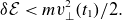 \begin{equation} \delta \mathcal{E} \lt m v_\perp ^2(t_1)/2 .\end{equation}
Figure 7(a) shows that the probability distribution of $\delta v_{\perp \mathcal{E}}$
, computed only for those particles satisfying (3.6), is marginally narrower than that of
$\delta v_{\perp \mathcal{E}}$
, computed only for those particles satisfying (3.6), is marginally narrower than that of $\delta v_\perp$
, as expected if non-adiabatic kicks are the main contribution to
$\delta v_\perp$
, as expected if non-adiabatic kicks are the main contribution to $\delta v_\perp$
.Footnote
5
$\delta v_\perp$
.Footnote
5
The ion diffusion $\langle \delta v_{\perp \mathcal{E}} \delta v_{\perp \mathcal{E}} \rangle /\delta t$
as a function of radius is shown in figure 7(b); its value is normalized to
$\langle \delta v_{\perp \mathcal{E}} \delta v_{\perp \mathcal{E}} \rangle /\delta t$
as a function of radius is shown in figure 7(b); its value is normalized to $v_{\mathrm{ti0}}^2 \Omega _{\mathrm{i0}}$
in all of figure 7(b–g). Here,
$v_{\mathrm{ti0}}^2 \Omega _{\mathrm{i0}}$
in all of figure 7(b–g). Here, $\langle \cdots \rangle$
is a velocity-distribution moment computed in radial bins. The use of
$\langle \cdots \rangle$
is a velocity-distribution moment computed in radial bins. The use of $\delta v_{\perp \mathcal{E}}$
decreases the measured diffusion as compared with
$\delta v_{\perp \mathcal{E}}$
decreases the measured diffusion as compared with $\langle \delta v_\perp \delta v_\perp \rangle /\delta t$
, as expected.
$\langle \delta v_\perp \delta v_\perp \rangle /\delta t$
, as expected.
The ion diffusion due to fluctuating fields $\delta E_\perp (\boldsymbol{r})$
can be described by a diffusion coefficient similar to those used in quasilinear models,
$\delta E_\perp (\boldsymbol{r})$
can be described by a diffusion coefficient similar to those used in quasilinear models,
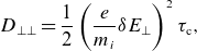 \begin{equation} D_{\perp \perp } = \frac {1}{2} \left ( \frac {e}{m_{{i}}} \delta E_\perp \right )^2 \tau _{\mathrm{c}} ,\end{equation}
where $\tau _{\mathrm{c}}$
is a yet-unknown wave–particle correlation time. Equation (3.7) assumes (i) weak but coherent kicks
$\tau _{\mathrm{c}}$
is a yet-unknown wave–particle correlation time. Equation (3.7) assumes (i) weak but coherent kicks $\delta v_\perp \approx (e/m_{{i}}) \delta E_\perp \tau _{\mathrm{c}}$
; (ii) a uniform random distribution of angles between
$\delta v_\perp \approx (e/m_{{i}}) \delta E_\perp \tau _{\mathrm{c}}$
; (ii) a uniform random distribution of angles between $\boldsymbol{v}_\perp$
and
$\boldsymbol{v}_\perp$
and $\delta \boldsymbol{E}_\perp$
to obtain a factor of
$\delta \boldsymbol{E}_\perp$
to obtain a factor of $1/2$
accounting for kicks in gyrophase instead of
$1/2$
accounting for kicks in gyrophase instead of $v_\perp$
magnitude. For a scattering-measurement time
$v_\perp$
magnitude. For a scattering-measurement time $\delta t \lt \tau _{\mathrm{c}}$
, we expect
$\delta t \lt \tau _{\mathrm{c}}$
, we expect
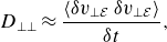 \begin{equation} D_{\perp \perp } \approx \frac { \langle \delta v_{\perp \mathcal{E}} \, \delta v_{\perp \mathcal{E}} \rangle }{ \delta t } ,\end{equation}
also replacing $\tau _{\mathrm{c}} \to \delta t$
in
$\tau _{\mathrm{c}} \to \delta t$
in $D_{\perp \perp }$
.
$D_{\perp \perp }$
.
Choosing $\delta t \lt \tau _{\mathrm{c}}$
is unusual for studies of particle diffusion, as the resulting (3.8) describes a more ‘ballistic’ than diffusive process. But, a short
$\delta t \lt \tau _{\mathrm{c}}$
is unusual for studies of particle diffusion, as the resulting (3.8) describes a more ‘ballistic’ than diffusive process. But, a short $\delta t$
helps us. When using a longer
$\delta t$
helps us. When using a longer $\delta t \gg \tau _{\mathrm{c}}$
, at least two issues arise. First, ions gyrate in and out of the scattering zone, as the zone’s radial width is similar to an ion Larmor radius. A typical ion may get one or a few kicks, gyrate out of the scattering zone and drift adiabatically, re-enter the scattering zone to be kicked again, and so on, resulting in a random walk with intermittent large time gaps. The scattering zone’s finite radial width may also introduce bias in the correlation time
$\delta t \gg \tau _{\mathrm{c}}$
, at least two issues arise. First, ions gyrate in and out of the scattering zone, as the zone’s radial width is similar to an ion Larmor radius. A typical ion may get one or a few kicks, gyrate out of the scattering zone and drift adiabatically, re-enter the scattering zone to be kicked again, and so on, resulting in a random walk with intermittent large time gaps. The scattering zone’s finite radial width may also introduce bias in the correlation time $\tau _{\mathrm{c}}$
, because a typical inboard (small
$\tau _{\mathrm{c}}$
, because a typical inboard (small $r$
) ion gyrating in and out of the scattering zone sees a redshift
$r$
) ion gyrating in and out of the scattering zone sees a redshift $\omega - k_\perp v_\perp$
, whereas a typical outboard (large
$\omega - k_\perp v_\perp$
, whereas a typical outboard (large $r$
) ion instead sees a blueshift
$r$
) ion instead sees a blueshift $\omega + k_\perp v_\perp$
. Second, a longer
$\omega + k_\perp v_\perp$
. Second, a longer $\delta t$
needed to sample multiple gyration periods
$\delta t$
needed to sample multiple gyration periods $2\pi \Omega _{\mathrm{i0}}^{-1}$
will introduce axial bounce effects. In the
$2\pi \Omega _{\mathrm{i0}}^{-1}$
will introduce axial bounce effects. In the $R_{{m}}=20$
simulation,
$R_{{m}}=20$
simulation, $\tau _{\mathrm{bounce}} \approx 40 \Omega _{\mathrm{i0}}^{-1}$
, and even fewer ion gyrations are executed within
$\tau _{\mathrm{bounce}} \approx 40 \Omega _{\mathrm{i0}}^{-1}$
, and even fewer ion gyrations are executed within $\tau _{\mathrm{bounce}}$
for the higher
$\tau _{\mathrm{bounce}}$
for the higher $R_{{m}}$
cases.
$R_{{m}}$
cases.
In figure 7(c) we compare (3.8) with the ion diffusion measured from individual particles. The fluctuating energy density is azimuth averaged as $\delta E_r^2 = \langle E_r^2 \rangle _\theta - {\langle E_r \rangle _\theta }^2$
, and similarly for
$\delta E_r^2 = \langle E_r^2 \rangle _\theta - {\langle E_r \rangle _\theta }^2$
, and similarly for $\delta E_\theta ^2$
; the sum
$\delta E_\theta ^2$
; the sum $\delta E_\perp ^2 = \delta E_\theta ^2 + \delta E_r^2$
. The diffusion due to
$\delta E_\perp ^2 = \delta E_\theta ^2 + \delta E_r^2$
. The diffusion due to $\delta E_\theta ^2$
agrees especially well with the particle measurement, whereas the diffusion due to
$\delta E_\theta ^2$
agrees especially well with the particle measurement, whereas the diffusion due to $\delta E_r^2$
agrees less well.
$\delta E_r^2$
agrees less well.
Numerical noise might drive axial losses from the plasma edge in the same way that we are attributing to DCLC, because PIC particle count decreases at the plasma edge. To check this possibility, figure 7(d) shows that the measured ion scattering is converged in the number of particles per cell used. We are confident that ion scattering is not due to numerical noise because (i) the DCLC electric fields have much larger energy density than numerical noise at the grid scale, and figure 7(c) shows good agreement in radial profiles of electric fields and scattering, (ii) we see weak to no $N_{\mathrm{ppc}}$
dependence of scattering rates, whereas if scattering were due to noise, we might expect either an outwards shift in
$N_{\mathrm{ppc}}$
dependence of scattering rates, whereas if scattering were due to noise, we might expect either an outwards shift in $r$
as
$r$
as $N_{\mathrm{ppc}}$
increases (for fixed DCLC amplitude), or a decrease in scattering rate if noise suppresses DCLC amplitude; (iii) ion scattering is clearly anisotropic (figure 7
a), whereas numerical scattering should be insensitive to
$N_{\mathrm{ppc}}$
increases (for fixed DCLC amplitude), or a decrease in scattering rate if noise suppresses DCLC amplitude; (iii) ion scattering is clearly anisotropic (figure 7
a), whereas numerical scattering should be insensitive to $v_\parallel$
versus
$v_\parallel$
versus $v_\perp$
because the grid scale is much smaller than the ion Larmor radius.
$v_\perp$
because the grid scale is much smaller than the ion Larmor radius.
In figure 7(e) we show the effect of $\delta t$
upon the radial profiles of measured ion diffusion. Figure 7(f) then samples the ion scattering at its radial peak
$\delta t$
upon the radial profiles of measured ion diffusion. Figure 7(f) then samples the ion scattering at its radial peak $r = 8.2 \;\mathrm{cm}$
(blue curve) and shows its dependence upon many more values of
$r = 8.2 \;\mathrm{cm}$
(blue curve) and shows its dependence upon many more values of $\delta t$
. We see that the diffusion moment scales linearly with small
$\delta t$
. We see that the diffusion moment scales linearly with small $\delta t$
as expected from (3.8); for comparison, the black dotted line shows an exactly linear correlation with
$\delta t$
as expected from (3.8); for comparison, the black dotted line shows an exactly linear correlation with $\delta t$
. As
$\delta t$
. As $\delta t$
becomes
$\delta t$
becomes $\gtrsim \Omega _{\mathrm{i0}}^{-1}$
, waves and particles decorrelate and the diffusion rate begins to fall. We perform a similar calculation at
$\gtrsim \Omega _{\mathrm{i0}}^{-1}$
, waves and particles decorrelate and the diffusion rate begins to fall. We perform a similar calculation at $(r,z) \approx (6.8,50) \;\mathrm{cm}$
(figure 7
f, orange curve) to conclude that
$(r,z) \approx (6.8,50) \;\mathrm{cm}$
(figure 7
f, orange curve) to conclude that $\tau _{\mathrm{c}}$
is shorter near the fast ion turning point. If
$\tau _{\mathrm{c}}$
is shorter near the fast ion turning point. If $\tau _{\mathrm{c}} \sim 1/\Omega _{{i}}$
(where
$\tau _{\mathrm{c}} \sim 1/\Omega _{{i}}$
(where $\Omega _{{i}}$
varies with
$\Omega _{{i}}$
varies with $z$
, unlike
$z$
, unlike $\Omega _{\mathrm{i0}}$
), the lower
$\Omega _{\mathrm{i0}}$
), the lower $\tau _{\mathrm{c}}$
can be easily explained by the
$\tau _{\mathrm{c}}$
can be easily explained by the $2\times$
increase in
$2\times$
increase in $B$
magnitude.
$B$
magnitude.
Finally, figure 7(g) shows $\langle \delta v_{\perp \mathcal{E}} \delta v_{\perp \mathcal{E}} \rangle /\delta t$
as a function of
$\langle \delta v_{\perp \mathcal{E}} \delta v_{\perp \mathcal{E}} \rangle /\delta t$
as a function of $(r,z)$
in the mirror’s central cell. The ion scattering at all
$(r,z)$
in the mirror’s central cell. The ion scattering at all $z$
is well localized to the same flux surfaces between beam-ion turning points. Scattering is strongest towards
$z$
is well localized to the same flux surfaces between beam-ion turning points. Scattering is strongest towards $z=0$
, where the central-cell field is relatively uniform.
$z=0$
, where the central-cell field is relatively uniform.
We conclude from figure 7(e,f) that particle scattering has a longer correlation time $\tau _{\mathrm{c}}$
and reaches a larger amplitude at the mirror midplane
$\tau _{\mathrm{c}}$
and reaches a larger amplitude at the mirror midplane $z=0$
, as compared with near the beam-ion turning points. Ions at
$z=0$
, as compared with near the beam-ion turning points. Ions at $z=0$
, and throughout the central cell where
$z=0$
, and throughout the central cell where $B \approx B(z=0)$
, should be more important for regulating DCLC growth and saturation than ions at the turning points.
$B \approx B(z=0)$
, should be more important for regulating DCLC growth and saturation than ions at the turning points.
3.4. Particle confinement time
Because the loss cone is full – i.e. $F(v_\perp )$
is roughly constant within the loss cone (figure 3) – our simulated mirrors are a collisionless analogue of the GDT at the Budker Institute (Ivanov & Prikhodko Reference Ivanov and Prikhodko2017). Ions scatter across the loss-cone boundary as fast as (or faster than) untrapped ions can stream out of the mirror, implying an effective mean free path shorter than the device’s length. The particle confinement time
$F(v_\perp )$
is roughly constant within the loss cone (figure 3) – our simulated mirrors are a collisionless analogue of the GDT at the Budker Institute (Ivanov & Prikhodko Reference Ivanov and Prikhodko2017). Ions scatter across the loss-cone boundary as fast as (or faster than) untrapped ions can stream out of the mirror, implying an effective mean free path shorter than the device’s length. The particle confinement time $\tau _{\mathrm{p}} \equiv N / |\mathrm{d} N/ \mathrm{d} t|$
, where
$\tau _{\mathrm{p}} \equiv N / |\mathrm{d} N/ \mathrm{d} t|$
, where $N$
is the total number of ions, then scales like the eponymous ‘gas dynamic’ time,
$N$
is the total number of ions, then scales like the eponymous ‘gas dynamic’ time,
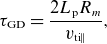 \begin{equation} \tau _{\mathrm{GD}} = \frac { 2 L_{\mathrm{p}} R_{{m}} } { v_{\mathrm{ti}\parallel } } ,\end{equation}
adapted from Endrizzi et al. (Reference Endrizzi2023, § 3) with $v_{\mathrm{ti}\parallel }$
a characteristic parallel thermal velocity.
$v_{\mathrm{ti}\parallel }$
a characteristic parallel thermal velocity.
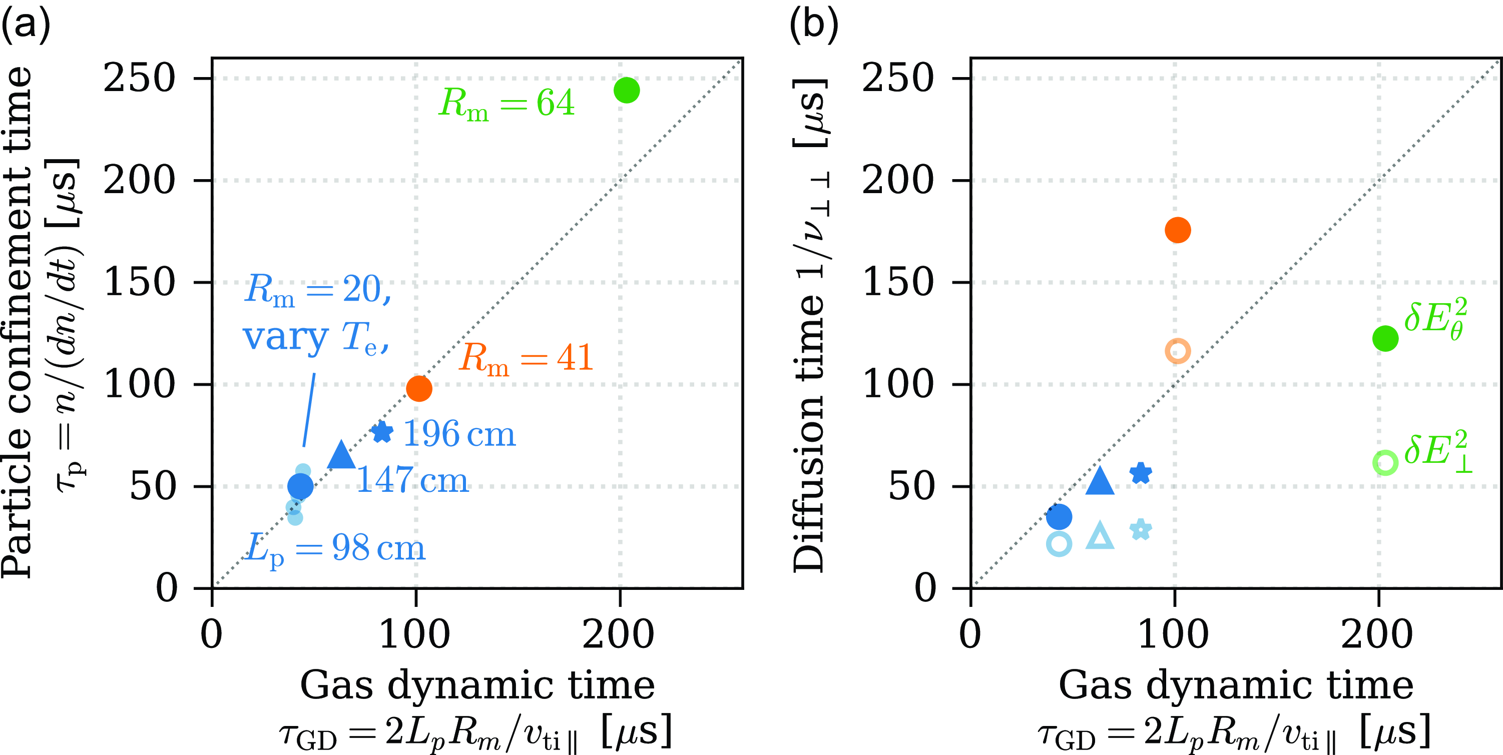
Figure 8. (a) Particle confinement time measured between $t=5$
to
$t=5$
to $6\tau _{\mathrm{bounce}}$
, for mirrors of varying
$6\tau _{\mathrm{bounce}}$
, for mirrors of varying $R_{{m}}$
(blue, orange, green) and device length
$R_{{m}}$
(blue, orange, green) and device length $L_{\mathrm{p}}$
(circle, triangle, star markers) as a function of
$L_{\mathrm{p}}$
(circle, triangle, star markers) as a function of $\tau _{\mathrm{GD}}$
(3.9). Small blue markers vary
$\tau _{\mathrm{GD}}$
(3.9). Small blue markers vary $T_{{e}}$
for
$T_{{e}}$
for $R_{{m}}=20$
; large blue marker is fiducial
$R_{{m}}=20$
; large blue marker is fiducial $T_{{e}}=1.25\;\mathrm{keV}$
. (b) Diffusion time scale
$T_{{e}}=1.25\;\mathrm{keV}$
. (b) Diffusion time scale $1/\nu _{\perp \perp }$
(3.10) modelled from
$1/\nu _{\perp \perp }$
(3.10) modelled from $\delta E_\theta ^2$
(solid markers) and
$\delta E_\theta ^2$
(solid markers) and $\delta E_\perp ^2$
(hollow markers), as a function of
$\delta E_\perp ^2$
(hollow markers), as a function of $\tau _{\mathrm{GD}}$
. In both panels, diagonal dotted line is
$\tau _{\mathrm{GD}}$
. In both panels, diagonal dotted line is $\tau _{\mathrm{p}} = \tau _{\mathrm{GD}}$
.
$\tau _{\mathrm{p}} = \tau _{\mathrm{GD}}$
.
To test the relation $\tau _{\mathrm{p}} \propto \tau _{\mathrm{GD}}$
, we measure
$\tau _{\mathrm{p}} \propto \tau _{\mathrm{GD}}$
, we measure $\tau _{\mathrm{p}}$
between
$\tau _{\mathrm{p}}$
between $t = 5$
to
$t = 5$
to $6\, \tau _{\mathrm{bounce}}$
, and
$6\, \tau _{\mathrm{bounce}}$
, and $v_{\mathrm{ti}\parallel } = \langle v_\parallel ^2 \rangle ^{1/2}$
at
$v_{\mathrm{ti}\parallel } = \langle v_\parallel ^2 \rangle ^{1/2}$
at $t=6\,\tau _{\mathrm{bounce}}$
, in each of the
$t=6\,\tau _{\mathrm{bounce}}$
, in each of the $R_{{m}}=\{20,41,64\}$
simulations with
$R_{{m}}=\{20,41,64\}$
simulations with $L_{\mathrm{p}} = 98 \;\mathrm{cm}$
on axis. We also measure
$L_{\mathrm{p}} = 98 \;\mathrm{cm}$
on axis. We also measure $\tau _{\mathrm{p}}$
and
$\tau _{\mathrm{p}}$
and $v_{\mathrm{ti}\parallel }$
in additional
$v_{\mathrm{ti}\parallel }$
in additional $R_{{m}} = 20$
simulations with varying
$R_{{m}} = 20$
simulations with varying $T_{{e}} = {0,2.5,5,10}$
keV and longer central cells (larger
$T_{{e}} = {0,2.5,5,10}$
keV and longer central cells (larger $L_{\mathrm{p}}$
); the latter are constructed as follows. Split the ‘original’ mirror device in half at
$L_{\mathrm{p}}$
); the latter are constructed as follows. Split the ‘original’ mirror device in half at $z=0$
. Between the mirror halves, insert a cylindrical plasma of length
$z=0$
. Between the mirror halves, insert a cylindrical plasma of length $98$
or
$98$
or $168$
cm, thereby increasing the entire mirror’s half-length
$168$
cm, thereby increasing the entire mirror’s half-length $L_{\mathrm{p}}$
by
$L_{\mathrm{p}}$
by $1.5$
or
$1.5$
or $2\times$
. The cylinder has, at all
$2\times$
. The cylinder has, at all $z$
, the same velocity distribution and magnetic field
$z$
, the same velocity distribution and magnetic field $\boldsymbol{B}$
as in the original mirror at
$\boldsymbol{B}$
as in the original mirror at $z=0$
. The simulation domain is made larger; mesh voxel dimensions (
$z=0$
. The simulation domain is made larger; mesh voxel dimensions ( $\Delta x$
,
$\Delta x$
, $\Delta y$
,
$\Delta y$
, $\Delta z$
) are the same as in § 2. The cylinder’s magnetic field is unphysical because it has
$\Delta z$
) are the same as in § 2. The cylinder’s magnetic field is unphysical because it has $\mathrm{d} B_z/\mathrm{d} r \ne 0$
and
$\mathrm{d} B_z/\mathrm{d} r \ne 0$
and $B_r = 0$
, implying non-zero current
$B_r = 0$
, implying non-zero current $c {\nabla }\times \boldsymbol{B}/(4\pi )$
, so we exclude this current from the
$c {\nabla }\times \boldsymbol{B}/(4\pi )$
, so we exclude this current from the $\boldsymbol{j} \times \boldsymbol{B}$
term in Ohm’s law(2.1).
$\boldsymbol{j} \times \boldsymbol{B}$
term in Ohm’s law(2.1).
The confinement time $\tau _{\mathrm{p}} \sim \mathcal{O}(10^2) \;\mathrm{\unicode{x03BC}s}$
, and
$\tau _{\mathrm{p}} \sim \mathcal{O}(10^2) \;\mathrm{\unicode{x03BC}s}$
, and $\tau _{\mathrm{p}}$
scales linearly with
$\tau _{\mathrm{p}}$
scales linearly with $\tau _{\mathrm{GD}}$
as expected (figure 8
a). Gas-dynamic confinement explains losses from the
$\tau _{\mathrm{GD}}$
as expected (figure 8
a). Gas-dynamic confinement explains losses from the $R_{{m}} = 20$
and
$R_{{m}} = 20$
and $41$
simulations very well. Raising electron temperature
$41$
simulations very well. Raising electron temperature $T_{{e}}$
from
$T_{{e}}$
from $0$
to
$0$
to $10 \;\mathrm{keV}$
lowers
$10 \;\mathrm{keV}$
lowers $\tau _{\mathrm{p}}$
from
$\tau _{\mathrm{p}}$
from $57$
to
$57$
to $35 \;\mathrm{\unicode{x03BC}s}$
for the
$35 \;\mathrm{\unicode{x03BC}s}$
for the $R_{{m}} = 20$
simulations. For comparison, the collisional (aka ‘classical’) confinement time is
$R_{{m}} = 20$
simulations. For comparison, the collisional (aka ‘classical’) confinement time is $0.1$
–
$0.1$
– $0.2 \;\mathrm{s}$
, using (3.4) of Endrizzi et al. (Reference Endrizzi2023) with
$0.2 \;\mathrm{s}$
, using (3.4) of Endrizzi et al. (Reference Endrizzi2023) with $n=3\times 10^{13}\;\mathrm{cm^{-3}}$
,
$n=3\times 10^{13}\;\mathrm{cm^{-3}}$
, $R_{{m}} = 20$
to
$R_{{m}} = 20$
to $64$
, and beam energy
$64$
, and beam energy $25\;\mathrm{keV}$
.
$25\;\mathrm{keV}$
.
The $R_{{m}} = 64$
shows 20 % better particle confinement than predicted by (3.9). Why? The larger plasma radius and hence longer flux-tube length
$R_{{m}} = 64$
shows 20 % better particle confinement than predicted by (3.9). Why? The larger plasma radius and hence longer flux-tube length $\gt 2 L_{\mathrm{p}}$
between mirror throats only explains
$\gt 2 L_{\mathrm{p}}$
between mirror throats only explains $\mathord {\sim } 5\,\%$
of the disagreement. We speculate that electrostatic potential effects may explain the remaining disagreement. In the
$\mathord {\sim } 5\,\%$
of the disagreement. We speculate that electrostatic potential effects may explain the remaining disagreement. In the $R_{{m}} =20,41$
cases, beam ions diffuse in
$R_{{m}} =20,41$
cases, beam ions diffuse in $v_\perp$
and escape with high
$v_\perp$
and escape with high $v_\parallel$
; electrostatic effects are weak since
$v_\parallel$
; electrostatic effects are weak since $T_{{e}} \ll T_{{i}}$
, so (3.9) accurately describes the beam ion confinement. The
$T_{{e}} \ll T_{{i}}$
, so (3.9) accurately describes the beam ion confinement. The $R_{{m}} = 64$
case has more cool, low-temperature ions (figure 3
i) that can be trapped by the sloshing-ions’ potential peak at
$R_{{m}} = 64$
case has more cool, low-temperature ions (figure 3
i) that can be trapped by the sloshing-ions’ potential peak at $z \sim 30 \;\mathrm{cm}$
(Kesner Reference Kesner1973, Reference Kesner1980); confinement is thus improved.
$z \sim 30 \;\mathrm{cm}$
(Kesner Reference Kesner1973, Reference Kesner1980); confinement is thus improved.
Instabilities in many settings are self-regulating; i.e. unstable waves drive phase-space flow that quenches the waves’ own energy source, driving the system to equilibrium (e.g. Kennel & Petschek Reference Kennel and Petschek1966). If DCLC self-regulates, then we may expect its amplitude to grow in time until the diffusion rate into the loss cone balances the axial outflow rate: $\nu _{\perp \perp } \propto \tau _{\mathrm{GD}}^{-1}$
. We test this by computing a diffusion rate into the loss cone as
$\nu _{\perp \perp } \propto \tau _{\mathrm{GD}}^{-1}$
. We test this by computing a diffusion rate into the loss cone as
 \begin{equation} \nu _{\perp \perp } \equiv \frac {1}{N_{\mathrm{\ell }}} \int \frac { D_{\perp \perp }(r) }{ {v_{\perp \mathrm{LC}}}^2 } n_{{i}}(r) 2\pi r \ell \,\mathrm{d} r , \end{equation}
which is a density-weighted average of $D_{\perp \perp }$
(3.7) over a cylindrical kernel of axial length
$D_{\perp \perp }$
(3.7) over a cylindrical kernel of axial length $\ell$
and radial profile
$\ell$
and radial profile $n_{{i}}(r)$
, normalized to
$n_{{i}}(r)$
, normalized to $N_{\mathrm{\ell }} = \int n_{{i}}(r) 2\pi r \ell \mathrm{d} r$
. We take
$N_{\mathrm{\ell }} = \int n_{{i}}(r) 2\pi r \ell \mathrm{d} r$
. We take $v_{\perp \mathrm{LC}} = v_{\mathrm{ti}\parallel }/\sqrt {R_{{m}} - 1}$
to approximate the ions’
$v_{\perp \mathrm{LC}} = v_{\mathrm{ti}\parallel }/\sqrt {R_{{m}} - 1}$
to approximate the ions’ $v_\perp$
at the loss cone boundary, we take
$v_\perp$
at the loss cone boundary, we take $\ell = 12 \;\mathrm{cm}$
centred at
$\ell = 12 \;\mathrm{cm}$
centred at $z=0$
, and we take
$z=0$
, and we take $\tau _{\mathrm{c}} = \Omega _{\mathrm{i0}}^{-1}$
. Given these assumptions, and given that (3.7) is not from a self-consistent quasilinear theory, we interpret (3.10) as no more accurate than an order-of-magnitude scaling. In figure 8(b) we compute the diffusion time scale
$\tau _{\mathrm{c}} = \Omega _{\mathrm{i0}}^{-1}$
. Given these assumptions, and given that (3.7) is not from a self-consistent quasilinear theory, we interpret (3.10) as no more accurate than an order-of-magnitude scaling. In figure 8(b) we compute the diffusion time scale $1/\nu _{\perp \perp }$
using either
$1/\nu _{\perp \perp }$
using either $\delta E_\theta ^2$
or
$\delta E_\theta ^2$
or $\delta E_\perp ^2$
as defined as in figure 7(c). We observe that
$\delta E_\perp ^2$
as defined as in figure 7(c). We observe that $1/\nu _{\perp \perp }$
has similar magnitude as
$1/\nu _{\perp \perp }$
has similar magnitude as $\tau _{\mathrm{GD}}$
, as expected. But, no trend is obvious from the scatter and few data points.
$\tau _{\mathrm{GD}}$
, as expected. But, no trend is obvious from the scatter and few data points.
4. Discussion
4.1. Cool plasma effects
How much cool plasma, and at what temperature, suppresses DCLC for the peaked beam-ion distributions injected into WHAM? To answer this, figure 9 computes DCLC linear stability with distinct ‘hot’ and ‘cool’ ion populations. The hot ions are a beam distribution at $t=0$
in our
$t=0$
in our $R_{{m}}=20$
simulation, taken from the midplane
$R_{{m}}=20$
simulation, taken from the midplane $z=0$
(figure 3
b), with
$z=0$
(figure 3
b), with $n_{\mathrm{hot}} = 4 \times 10^{12} \;\mathrm{cm^{-3}}$
. The cool ions are a Maxwellian of the same species (deuterium), with density
$n_{\mathrm{hot}} = 4 \times 10^{12} \;\mathrm{cm^{-3}}$
. The cool ions are a Maxwellian of the same species (deuterium), with density $n_{\mathrm{cool}}$
and temperature
$n_{\mathrm{cool}}$
and temperature $T_{\mathrm{cool}}$
. We solve (3.4) using the same procedure as in § 3.2, within a finite domain
$T_{\mathrm{cool}}$
. We solve (3.4) using the same procedure as in § 3.2, within a finite domain $k\rho _{\mathrm{i0}} \lt 15$
,
$k\rho _{\mathrm{i0}} \lt 15$
, $\textrm {Re}(\omega )/\Omega _{\mathrm{i0}} \lt 10$
, and
$\textrm {Re}(\omega )/\Omega _{\mathrm{i0}} \lt 10$
, and $\textrm {Im}(\omega )/\Omega _{\mathrm{i0}} \lt 4$
.
$\textrm {Im}(\omega )/\Omega _{\mathrm{i0}} \lt 4$
.
Figure 9. Effect of cool plasma on DCLC linear stability in WHAM with $R_{{m}}=20$
and a hot beam-ion distribution. (a): The 2-D regime map of maximum growth rate
$R_{{m}}=20$
and a hot beam-ion distribution. (a): The 2-D regime map of maximum growth rate $\textrm {Im}(\omega )/\Omega _{\mathrm{i0}}$
as a function of
$\textrm {Im}(\omega )/\Omega _{\mathrm{i0}}$
as a function of $n_{\mathrm{cool}}$
and
$n_{\mathrm{cool}}$
and $T_{\mathrm{cool}}$
. (b) Like (a), but showing minimum
$T_{\mathrm{cool}}$
. (b) Like (a), but showing minimum $\textrm {Re}(\omega )/\Omega _{\mathrm{i0}}$
that is DCLC unstable. As cool plasma density is raised, low harmonics are stabilized. White pixels in (b), at
$\textrm {Re}(\omega )/\Omega _{\mathrm{i0}}$
that is DCLC unstable. As cool plasma density is raised, low harmonics are stabilized. White pixels in (b), at $T_{\mathrm{cool}} \sim 5 \;\mathrm{keV}$
and
$T_{\mathrm{cool}} \sim 5 \;\mathrm{keV}$
and $\log _{10}(n_{\mathrm{cool}}/n_{\mathrm{hot}}) \sim 0$
, mean that no linearly unstable modes were found. (c) Example ion distribution
$\log _{10}(n_{\mathrm{cool}}/n_{\mathrm{hot}}) \sim 0$
, mean that no linearly unstable modes were found. (c) Example ion distribution $F(v_\perp )$
with
$F(v_\perp )$
with $1 \;\mathrm{keV}$
cool plasma (dotted blue) added to initial
$1 \;\mathrm{keV}$
cool plasma (dotted blue) added to initial $R_{{m}}=20$
distribution. (d) Dispersion relation solutions corresponding to (c), showing normal modes (black), unstable mode
$R_{{m}}=20$
distribution. (d) Dispersion relation solutions corresponding to (c), showing normal modes (black), unstable mode $\textrm {Re}(\omega )$
(blue) and unstable mode
$\textrm {Re}(\omega )$
(blue) and unstable mode $\textrm {Im}(\omega )$
(green). (e, f) Like (c, d), but with
$\textrm {Im}(\omega )$
(green). (e, f) Like (c, d), but with $4.9 \;\mathrm{keV}$
cool plasma. (g, h) Like (c, d), but with
$4.9 \;\mathrm{keV}$
cool plasma. (g, h) Like (c, d), but with $9.0 \;\mathrm{keV}$
cool plasma.
$9.0 \;\mathrm{keV}$
cool plasma.
Figure 10. Effect of cool plasma on particle losses and density fluctuations in Hybrid-VPIC simulations with $R_{{m}}=20$
. (a) Initial density radial profiles for hot (black) and cool (coloured) ions. (b) Total number of hot ions within simulation domain, normalized to initial value, for varying
$R_{{m}}=20$
. (a) Initial density radial profiles for hot (black) and cool (coloured) ions. (b) Total number of hot ions within simulation domain, normalized to initial value, for varying $n_{\mathrm{cool}}$
at fixed
$n_{\mathrm{cool}}$
at fixed $T_{\mathrm{cool}}=1\;\mathrm{keV}$
. (c) Like panel (b), but for cool ions. (d) Particle confinement time
$T_{\mathrm{cool}}=1\;\mathrm{keV}$
. (c) Like panel (b), but for cool ions. (d) Particle confinement time $\tau _{\mathrm{p}} = N/(\mathrm{d} N/\mathrm{d} t)$
for hot and cool populations, same simulations as in (b) and (c). (e) Fourier spectra of azimuthal density fluctuations, using total (hot plus cool) ion population; solid lines are median and shading is 25–75 percentile range within
$\tau _{\mathrm{p}} = N/(\mathrm{d} N/\mathrm{d} t)$
for hot and cool populations, same simulations as in (b) and (c). (e) Fourier spectra of azimuthal density fluctuations, using total (hot plus cool) ion population; solid lines are median and shading is 25–75 percentile range within $3$
–
$3$
– $6\;\mathrm{\unicode{x03BC}s}$
. (f)–(i) Like (b)–(e), but emphasis on varying
$6\;\mathrm{\unicode{x03BC}s}$
. (f)–(i) Like (b)–(e), but emphasis on varying $T_{\mathrm{cool}} = \{1,2,5\} \;\mathrm{keV}$
at fixed
$T_{\mathrm{cool}} = \{1,2,5\} \;\mathrm{keV}$
at fixed $n_{\mathrm{cool}}$
. Curve styles are matched across all panels.
$n_{\mathrm{cool}}$
. Curve styles are matched across all panels.
Figure 9(a) predicts that DCLC is suppressed when cool and hot ion densities are nearly equal, and $T_{\mathrm{cool}} \sim 2$
to
$T_{\mathrm{cool}} \sim 2$
to $10 \;\mathrm{keV}$
. In cases where DCLC is not fully stabilized, figure 9(b) shows that dense-enough cold plasma will at least stabilize low cyclotron harmonics; we anticipate that the remaining unstable high harmonics may have weaker scattering rate. Figure 9(b) qualitatively concurs with recent measurements on the GDT device: DCLC at high harmonics appeared when a relatively high gas density was puffed into GDT’s central chamber before neutral-beam injection (Prikhodko et al. Reference Prikhodko2018; Shmigelsky et al. Reference Shmigelsky, Meyster, Chernoshtanov, Lizunov, Solomakhin and Yakovlev2024); critically, this form of DCLC did not impede the build-up of plasma pressure. Figure 9(c–h) show the effect of varying
$10 \;\mathrm{keV}$
. In cases where DCLC is not fully stabilized, figure 9(b) shows that dense-enough cold plasma will at least stabilize low cyclotron harmonics; we anticipate that the remaining unstable high harmonics may have weaker scattering rate. Figure 9(b) qualitatively concurs with recent measurements on the GDT device: DCLC at high harmonics appeared when a relatively high gas density was puffed into GDT’s central chamber before neutral-beam injection (Prikhodko et al. Reference Prikhodko2018; Shmigelsky et al. Reference Shmigelsky, Meyster, Chernoshtanov, Lizunov, Solomakhin and Yakovlev2024); critically, this form of DCLC did not impede the build-up of plasma pressure. Figure 9(c–h) show the effect of varying $T_{\mathrm{cool}}$
(with
$T_{\mathrm{cool}}$
(with $n_{\mathrm{cool}} = n_{\mathrm{hot}}$
) upon DCLC mode structure in
$n_{\mathrm{cool}} = n_{\mathrm{hot}}$
) upon DCLC mode structure in $(\omega ,k)$
. As
$(\omega ,k)$
. As $T_{\mathrm{cool}}$
rises, quenching of low harmonics proceeds to total stabilization. When
$T_{\mathrm{cool}}$
rises, quenching of low harmonics proceeds to total stabilization. When $T_{\mathrm{cool}}$
is too high and near the beam ions’ effective temperature, the ‘cool’ plasma is less able to reduce the velocity-space gradient
$T_{\mathrm{cool}}$
is too high and near the beam ions’ effective temperature, the ‘cool’ plasma is less able to reduce the velocity-space gradient $\mathrm{d} F/\mathrm{d} v_\perp$
and DCLC becomes unstable at all harmonics.
$\mathrm{d} F/\mathrm{d} v_\perp$
and DCLC becomes unstable at all harmonics.
To test the predictions of figure 9, we repeat the $R_{{m}}=20$
Hybrid-VPIC simulation with cool plasma added to the radial edge, varying
$R_{{m}}=20$
Hybrid-VPIC simulation with cool plasma added to the radial edge, varying $n_{\mathrm{cool}} \approx \{ 4, 8, 16 \} \times 10^{12} \;\mathrm{cm^{-3}}$
within radii
$n_{\mathrm{cool}} \approx \{ 4, 8, 16 \} \times 10^{12} \;\mathrm{cm^{-3}}$
within radii $r \sim 5$
to
$r \sim 5$
to $12 \;\mathrm{cm}$
(figure 10
a) and also varying
$12 \;\mathrm{cm}$
(figure 10
a) and also varying $T_{\mathrm{cool}} = \{ 1, 2, 5 \} \;\mathrm{keV}$
. The simulation results are summarized in figure 10(b–i).
$T_{\mathrm{cool}} = \{ 1, 2, 5 \} \;\mathrm{keV}$
. The simulation results are summarized in figure 10(b–i).
Cool $1\;\mathrm{keV}$
plasma quenches DCLC losses and improves the hot plasma’s final
$1\;\mathrm{keV}$
plasma quenches DCLC losses and improves the hot plasma’s final $N/N(t=0)$
by a factor of
$N/N(t=0)$
by a factor of $\mathord {\sim } 2$
to
$\mathord {\sim } 2$
to $5\times$
(figure 10
b). The hot plasma’s final confinement time is at most
$5\times$
(figure 10
b). The hot plasma’s final confinement time is at most $\tau _{\mathrm{p}} = 445 \;\mathrm{\unicode{x03BC}s}$
, a stark improvement over
$\tau _{\mathrm{p}} = 445 \;\mathrm{\unicode{x03BC}s}$
, a stark improvement over $\tau _{\mathrm{p}} = 50 \;\mathrm{\unicode{x03BC}s}$
without cool plasma (figure 10
d). The cool plasma itself is less well confined with
$\tau _{\mathrm{p}} = 50 \;\mathrm{\unicode{x03BC}s}$
without cool plasma (figure 10
d). The cool plasma itself is less well confined with $\tau _{\mathrm{p}} \lesssim 200 \;\mathrm{\unicode{x03BC}s}$
(figure 10
d), but it may be externally replenished in real experiments or in more realistic future simulations. The simulation with lowest
$\tau _{\mathrm{p}} \lesssim 200 \;\mathrm{\unicode{x03BC}s}$
(figure 10
d), but it may be externally replenished in real experiments or in more realistic future simulations. The simulation with lowest $n_{\mathrm{cool}} = 4 \times 10^{12} \;\mathrm{cm^{-3}}$
shows that cool ions are better confined than the hot ions, qualitatively consistent with trapping by the sloshing ions’ axial potential (figure 10
b,c). The situation reverses at higher
$n_{\mathrm{cool}} = 4 \times 10^{12} \;\mathrm{cm^{-3}}$
shows that cool ions are better confined than the hot ions, qualitatively consistent with trapping by the sloshing ions’ axial potential (figure 10
b,c). The situation reverses at higher $n_{\mathrm{cool}}$
: hot ions become better confined than cool ions, which we speculate may be due to flattening of ion density
$n_{\mathrm{cool}}$
: hot ions become better confined than cool ions, which we speculate may be due to flattening of ion density $n$
, and hence also electric potential
$n$
, and hence also electric potential $\phi$
, along
$\phi$
, along $z$
.
$z$
.
Azimuthal fluctuations in density confirm that cool plasma quenches DCLC at $m \approx 10$
(figure 10
e). But, cool ions also drive faster-growing MHD interchange-like modes at
$m \approx 10$
(figure 10
e). But, cool ions also drive faster-growing MHD interchange-like modes at $m \approx 4$
. If our simulations were run longer than
$m \approx 4$
. If our simulations were run longer than $t = 6 \;\mathrm{\unicode{x03BC}s}$
, these interchanges might eventually cause large ion losses. In laboratory devices, interchange can be stabilized by shear flow driven by either external voltage biasing (Beklemishev et al. Reference Beklemishev, Bagryansky, Chaschin and Soldatkina2010; Yakovlev et al. Reference Yakovlev, Shalashov, Gospodchikov, Maximov, Prikhodko, Savkin, Soldatkina, Solomakhin and Bagryansky2018) or electron cyclotron heating (Yoshikawa et al. Reference Yoshikawa2019). We thus remain optimistic that cool plasma stabilization can work in WHAM, especially given the method’s success in real laboratory experiments (Coensgen et al. Reference Coensgen, Cummins, Logan, Molvik, Nexsen, Simonen, Stallard and Turner1975; Shmigelsky et al. Reference Shmigelsky, Meyster, Chernoshtanov, Lizunov, Solomakhin and Yakovlev2024). In § 4.4, we will comment further on interchange identification and growth/suppression.
$t = 6 \;\mathrm{\unicode{x03BC}s}$
, these interchanges might eventually cause large ion losses. In laboratory devices, interchange can be stabilized by shear flow driven by either external voltage biasing (Beklemishev et al. Reference Beklemishev, Bagryansky, Chaschin and Soldatkina2010; Yakovlev et al. Reference Yakovlev, Shalashov, Gospodchikov, Maximov, Prikhodko, Savkin, Soldatkina, Solomakhin and Bagryansky2018) or electron cyclotron heating (Yoshikawa et al. Reference Yoshikawa2019). We thus remain optimistic that cool plasma stabilization can work in WHAM, especially given the method’s success in real laboratory experiments (Coensgen et al. Reference Coensgen, Cummins, Logan, Molvik, Nexsen, Simonen, Stallard and Turner1975; Shmigelsky et al. Reference Shmigelsky, Meyster, Chernoshtanov, Lizunov, Solomakhin and Yakovlev2024). In § 4.4, we will comment further on interchange identification and growth/suppression.
The Hybrid-VPIC simulations quench DCLC losses at higher $n_{\mathrm{cool}}/n_{\mathrm{hot}}$
and lower
$n_{\mathrm{cool}}/n_{\mathrm{hot}}$
and lower $T_{\mathrm{cool}}$
than predicted by the linear theory. The hot-ion confinement is worse with
$T_{\mathrm{cool}}$
than predicted by the linear theory. The hot-ion confinement is worse with $T_{\mathrm{cool}} = 5 \;\mathrm{keV}$
as compared with lower
$T_{\mathrm{cool}} = 5 \;\mathrm{keV}$
as compared with lower $T_{\mathrm{cool}}$
(figure 10
f–h), which contrasts with the prediction of figure 9 that
$T_{\mathrm{cool}}$
(figure 10
f–h), which contrasts with the prediction of figure 9 that $T_{\mathrm{cool}} = 5 \;\mathrm{keV}$
with
$T_{\mathrm{cool}} = 5 \;\mathrm{keV}$
with $n_{\mathrm{cool}} \approx n_{\mathrm{hot}}$
fully stabilizes DCLC within a wide
$n_{\mathrm{cool}} \approx n_{\mathrm{hot}}$
fully stabilizes DCLC within a wide $(k,\textrm {Re}(\omega ),\textrm {Im}(\omega ))$
domain. Why does
$(k,\textrm {Re}(\omega ),\textrm {Im}(\omega ))$
domain. Why does $T_{\mathrm{cool}} \sim 1 \;\mathrm{keV}$
work better than
$T_{\mathrm{cool}} \sim 1 \;\mathrm{keV}$
work better than $5 \;\mathrm{keV}$
? It may be explained by some combination of (i) weaker electrostatic trapping and faster outflow
$5 \;\mathrm{keV}$
? It may be explained by some combination of (i) weaker electrostatic trapping and faster outflow $v_{\mathrm{ti\parallel }}$
as
$v_{\mathrm{ti\parallel }}$
as $T_{\mathrm{cool}}$
increases, and (ii) quasilinear diffusion of beam ions towards the loss cone, which shifts the unstable drive
$T_{\mathrm{cool}}$
increases, and (ii) quasilinear diffusion of beam ions towards the loss cone, which shifts the unstable drive $\mathrm{d} F/\mathrm{d} v_\perp$
to lower
$\mathrm{d} F/\mathrm{d} v_\perp$
to lower $v_\perp$
so that lower
$v_\perp$
so that lower $T_{\mathrm{cool}}$
becomes stabilizing.
$T_{\mathrm{cool}}$
becomes stabilizing.
Let us expand on point (ii). For a quasilinearly diffused $F(v_\perp )$
, the relevant
$F(v_\perp )$
, the relevant $T_{\mathrm{cool}}$
is set not by the injected beam distribution, but instead by the loss-cone’s
$T_{\mathrm{cool}}$
is set not by the injected beam distribution, but instead by the loss-cone’s $v_\perp$
boundary value at the injected beam’s characteristic
$v_\perp$
boundary value at the injected beam’s characteristic $v_\parallel$
. For WHAM’s
$v_\parallel$
. For WHAM’s $45^\circ$
pitch-angle beam, DCLC-scattered ions escape at the loss-cone boundary with perpendicular energy,
$45^\circ$
pitch-angle beam, DCLC-scattered ions escape at the loss-cone boundary with perpendicular energy,
 \begin{equation} m_{{i}} v_\perp ^2 / 2 \sim E_{\mathrm{beam}} \cos ^2\theta _{{NBI}}/(R_{{m}}-1) \approx 0.7 \;\mathrm{keV} ,\end{equation}
using $E_{\mathrm{beam}} = 25 \;\mathrm{keV}$
,
$E_{\mathrm{beam}} = 25 \;\mathrm{keV}$
, $\theta _{{NBI}} = 45^\circ$
, and
$\theta _{{NBI}} = 45^\circ$
, and $R_{{m}}=20$
. Equation (4.1) agrees with the
$R_{{m}}=20$
. Equation (4.1) agrees with the $T_{\mathrm{cool}} = 1 \;\mathrm{keV}$
stabilization in our simulations (figure 10).
$T_{\mathrm{cool}} = 1 \;\mathrm{keV}$
stabilization in our simulations (figure 10).
It is interesting to contrast WHAM with 2XIIB, which used $90^\circ$
pitch-angle beam injection. In 2XIIB, DCLC-scattered ions have
$90^\circ$
pitch-angle beam injection. In 2XIIB, DCLC-scattered ions have $v_\parallel \sim 0$
and therefore escape at the loss-cone boundary with perpendicular energy
$v_\parallel \sim 0$
and therefore escape at the loss-cone boundary with perpendicular energy
 \begin{equation} m_{{i}} v_\perp ^2 / 2 \sim q_{{i}} \Delta \phi /(R_{{m}} - 1) \sim 0.2-0.5 \;\mathrm{keV} \end{equation}
using $q_{{i}} \Delta \phi \sim (2-5) \times T_{{e}}$
,
$q_{{i}} \Delta \phi \sim (2-5) \times T_{{e}}$
, $T_{{e}} \approx 100 \;\mathrm{eV}$
and
$T_{{e}} \approx 100 \;\mathrm{eV}$
and $R_{{m}} = 2$
(Coensgen et al. 1975); here
$R_{{m}} = 2$
(Coensgen et al. 1975); here $\Delta \phi$
is the axial potential drop from midplane to throat (Baldwin Reference Baldwin1977, § V.B). So, we may bear in mind that the appropriate
$\Delta \phi$
is the axial potential drop from midplane to throat (Baldwin Reference Baldwin1977, § V.B). So, we may bear in mind that the appropriate $T_{\mathrm{cool}}$
to stabilize DCLC (and the parametric dependence of
$T_{\mathrm{cool}}$
to stabilize DCLC (and the parametric dependence of $T_{\mathrm{cool}}$
upon either
$T_{\mathrm{cool}}$
upon either $E_{\mathrm{beam}}$
or
$E_{\mathrm{beam}}$
or $\Delta \phi$
) is mediated by the beam injection angle in a given device.
$\Delta \phi$
) is mediated by the beam injection angle in a given device.
4.2. Spatial gradient effects
A smaller spatial gradient $\epsilon \rho _{\mathrm{i0}}$
also helps to stabilize DCLC (Baldwin Reference Baldwin1977; Correll et al. Reference Correll, Clauser, Coensgen, Cummins, Drake, Foote, Futch, Goodman, Grubb and Melin1980; Ferron & Wong Reference Ferron and Wong1984). Figure 11 shows this for plasma parameters similar to the physically larger, break-even axisymmetric mirror (BEAM) design concept of Forest et al. (Reference Forest2024). We recompute DCLC linear stability for BEAM’s radial edge comprising (i) hot deuterium and tritium beam ions, with equal densities of deuterium and tritium, and temperature
$\epsilon \rho _{\mathrm{i0}}$
also helps to stabilize DCLC (Baldwin Reference Baldwin1977; Correll et al. Reference Correll, Clauser, Coensgen, Cummins, Drake, Foote, Futch, Goodman, Grubb and Melin1980; Ferron & Wong Reference Ferron and Wong1984). Figure 11 shows this for plasma parameters similar to the physically larger, break-even axisymmetric mirror (BEAM) design concept of Forest et al. (Reference Forest2024). We recompute DCLC linear stability for BEAM’s radial edge comprising (i) hot deuterium and tritium beam ions, with equal densities of deuterium and tritium, and temperature $T \approx 60 \;\mathrm{keV}$
(Forest et al. Reference Forest2024, figure 6), and (ii) cool Maxwellian ions with varying
$T \approx 60 \;\mathrm{keV}$
(Forest et al. Reference Forest2024, figure 6), and (ii) cool Maxwellian ions with varying $n_{\mathrm{cool}}$
,
$n_{\mathrm{cool}}$
, $T_{\mathrm{cool}}$
and isotope choice of hydrogen, deuterium, tritium or a deuterium–tritium mixture (equal densities of deuterium and tritium). The stability calculation assumes
$T_{\mathrm{cool}}$
and isotope choice of hydrogen, deuterium, tritium or a deuterium–tritium mixture (equal densities of deuterium and tritium). The stability calculation assumes $\epsilon \rho _{\mathrm{i0}} = -0.04$
,
$\epsilon \rho _{\mathrm{i0}} = -0.04$
, $B = 3 \;\mathrm{T}$
and
$B = 3 \;\mathrm{T}$
and $n_{\mathrm{hot}} = 6 \times 10^{13} \;\mathrm{cm^{-3}}$
counting both deuterium and tritium species. The value
$n_{\mathrm{hot}} = 6 \times 10^{13} \;\mathrm{cm^{-3}}$
counting both deuterium and tritium species. The value $1/|\epsilon \rho _{\mathrm{i0}}| = 25$
approximately matches the DCLC design constraint
$1/|\epsilon \rho _{\mathrm{i0}}| = 25$
approximately matches the DCLC design constraint $a/\rho _{{i}} = 25$
used by both Forest et al. (Reference Forest2024) and Frank et al. Reference Frank2025. For normalization, we take
$a/\rho _{{i}} = 25$
used by both Forest et al. (Reference Forest2024) and Frank et al. Reference Frank2025. For normalization, we take $\rho _{\mathrm{i0}} = 1.2 \;\mathrm{cm}$
and
$\rho _{\mathrm{i0}} = 1.2 \;\mathrm{cm}$
and $f_{\mathrm{ci0}} = 22.9 \;\mathrm{MHz}$
. We solve (3.4) using the same procedure as in § 3.2, within a finite domain
$f_{\mathrm{ci0}} = 22.9 \;\mathrm{MHz}$
. We solve (3.4) using the same procedure as in § 3.2, within a finite domain $k\rho _{\mathrm{i0}} \lt 30$
,
$k\rho _{\mathrm{i0}} \lt 30$
, $\textrm {Re}(\omega )/\Omega _{\mathrm{i0}} \lt 10$
and
$\textrm {Re}(\omega )/\Omega _{\mathrm{i0}} \lt 10$
and $\textrm {Im}(\omega )/\Omega _{\mathrm{i0}} \lt 5$
. The domain is larger than before because DCLC appears at larger
$\textrm {Im}(\omega )/\Omega _{\mathrm{i0}} \lt 5$
. The domain is larger than before because DCLC appears at larger $k \rho _{\mathrm{i0}}$
; the relevant
$k \rho _{\mathrm{i0}}$
; the relevant $k$
may be estimated for the
$k$
may be estimated for the $n$
th cyclotron harmonic as
$n$
th cyclotron harmonic as $k \rho _{\mathrm{i0}} \approx n/(|\epsilon | \rho _{\mathrm{i0}})/(T_{\mathrm{i\perp }}/T_{\mathrm{i0}})$
, from requiring that the ion diamagnetic drift
$k \rho _{\mathrm{i0}} \approx n/(|\epsilon | \rho _{\mathrm{i0}})/(T_{\mathrm{i\perp }}/T_{\mathrm{i0}})$
, from requiring that the ion diamagnetic drift $\omega /k = v_{\mathrm{Di}}$
intersects the harmonics
$\omega /k = v_{\mathrm{Di}}$
intersects the harmonics $\omega = n\Omega _{\mathrm{i0}}$
. The Bessel sums retain all terms with index
$\omega = n\Omega _{\mathrm{i0}}$
. The Bessel sums retain all terms with index $|n| \leqslant 120$
to ensure convergence.
$|n| \leqslant 120$
to ensure convergence.

Figure 11. Effect of cool plasma on DCLC linear stability in a physically larger next-step mirror, similar to the BEAM concept described in Forest et al. (Reference Forest2024), with spatial gradient $|\epsilon | \rho _{\mathrm{i0}} = 0.04$
smaller than in WHAM. Each panel shows varying cool plasma composition. For the cool D * T case,
$|\epsilon | \rho _{\mathrm{i0}} = 0.04$
smaller than in WHAM. Each panel shows varying cool plasma composition. For the cool D * T case, $n_{\mathrm{cool}}$
counts both D/T species, and the cool D and cool T have equal densities. Total stabilization
$n_{\mathrm{cool}}$
counts both D/T species, and the cool D and cool T have equal densities. Total stabilization $\textrm {Im}(\omega ) \to 0$
is achieved when the cool ions’ isotopes are matched to that of the hot ions. Colourmap range in
$\textrm {Im}(\omega ) \to 0$
is achieved when the cool ions’ isotopes are matched to that of the hot ions. Colourmap range in $\textrm {Im}(\omega )$
is reduced from figure 9(a).
$\textrm {Im}(\omega )$
is reduced from figure 9(a).
Figure 11 predicts that a larger region of the parameter space $(n_{\mathrm{cool}}/n_{\mathrm{hot}}, T_{\mathrm{cool}}/T_{\mathrm{hot}})$
becomes available to help stabilize DCLC in a BEAM-like concept. Complete stabilization
$(n_{\mathrm{cool}}/n_{\mathrm{hot}}, T_{\mathrm{cool}}/T_{\mathrm{hot}})$
becomes available to help stabilize DCLC in a BEAM-like concept. Complete stabilization $\textrm {Im}(\omega ) \to 0$
occurs when the cool plasma is a deuterium–tritium mixture like the hot plasma, following the empirical ‘spectral rule’ of Kotelnikov & Chernoshtanov (Reference Kotelnikov and Chernoshtanov2018). For cool plasma of pure hydrogen, deuterium or tritium, we find that
$\textrm {Im}(\omega ) \to 0$
occurs when the cool plasma is a deuterium–tritium mixture like the hot plasma, following the empirical ‘spectral rule’ of Kotelnikov & Chernoshtanov (Reference Kotelnikov and Chernoshtanov2018). For cool plasma of pure hydrogen, deuterium or tritium, we find that $\textrm {Im}(\omega )$
is reduced but generally remains non-zero; the remaining unstable modes have
$\textrm {Im}(\omega )$
is reduced but generally remains non-zero; the remaining unstable modes have $\omega$
at the hot-ion cyclotron harmonics not overlapped by the cool-ion harmonics, as previously shown by Kotelnikov & Chernoshtanov (Reference Kotelnikov and Chernoshtanov2018).
$\omega$
at the hot-ion cyclotron harmonics not overlapped by the cool-ion harmonics, as previously shown by Kotelnikov & Chernoshtanov (Reference Kotelnikov and Chernoshtanov2018).
Both Tang et al. (Reference Tang, Pearlstein and Berk1972, figure 1) and Baldwin (1977, figure 7) also computed the maximum radial gradient $\epsilon$
for DCLC to be stable, as a function of the density-proxy parameter
$\epsilon$
for DCLC to be stable, as a function of the density-proxy parameter $(\Omega _{{i}}/\omega _{\mathrm{pi}})^2$
. For WHAM,
$(\Omega _{{i}}/\omega _{\mathrm{pi}})^2$
. For WHAM, $\epsilon \rho _{\mathrm{i0}} \sim 1$
is DCLC unstable for nearly all values of
$\epsilon \rho _{\mathrm{i0}} \sim 1$
is DCLC unstable for nearly all values of $(\Omega _{{i}}/\omega _{\mathrm{pi}})^2$
anyway. For the model BEAM plasma in figure 11, we find
$(\Omega _{{i}}/\omega _{\mathrm{pi}})^2$
anyway. For the model BEAM plasma in figure 11, we find $(\Omega _{{i}}/\omega _{\mathrm{pi}})^2 \sim 3 \times 10^{-4}$
requires low
$(\Omega _{{i}}/\omega _{\mathrm{pi}})^2 \sim 3 \times 10^{-4}$
requires low $\epsilon \rho _{\mathrm{i0}} \sim 0.01$
for stability, so it is reasonable that our model with
$\epsilon \rho _{\mathrm{i0}} \sim 0.01$
for stability, so it is reasonable that our model with $|\epsilon \rho _{\mathrm{i0}}| \sim 0.04$
remains DCLC unstable in the absence of cool plasma.
$|\epsilon \rho _{\mathrm{i0}}| \sim 0.04$
remains DCLC unstable in the absence of cool plasma.
Though figure 11 suggests that a BEAM-like concept may be DCLC unstable, we note that many mitigating factors remain. First, BEAM-sized plasmas need much lower $n_{\mathrm{cool}}$
to stabilize DCLC as compared with WHAM, as expected from previous work (Baldwin Reference Baldwin1977); there are many ways to craft such cool plasma in the laboratory. Second, the peaked beam-ion distributions used here may be viewed as ‘maximally’ unstable; quasilinear diffusion will smooth ion distributions towards marginal stability, as discussed in §§ 3.4 and 4.1. Third, our calculation neglects physical effects such as finite plasma
$n_{\mathrm{cool}}$
to stabilize DCLC as compared with WHAM, as expected from previous work (Baldwin Reference Baldwin1977); there are many ways to craft such cool plasma in the laboratory. Second, the peaked beam-ion distributions used here may be viewed as ‘maximally’ unstable; quasilinear diffusion will smooth ion distributions towards marginal stability, as discussed in §§ 3.4 and 4.1. Third, our calculation neglects physical effects such as finite plasma $\beta$
(i.e.
$\beta$
(i.e. ${\nabla } B$
along
${\nabla } B$
along $r$
) and both radial and axial geometry; these effects are generally thought to aid stability (Tang et al. Reference Tang, Pearlstein and Berk1972). Fourth, recall from figure 9 that even if DCLC remains unstable, it can be rendered less harmful by pushing
$r$
) and both radial and axial geometry; these effects are generally thought to aid stability (Tang et al. Reference Tang, Pearlstein and Berk1972). Fourth, recall from figure 9 that even if DCLC remains unstable, it can be rendered less harmful by pushing $\textrm {Re}(\omega )$
to high harmonics of
$\textrm {Re}(\omega )$
to high harmonics of $\Omega _{\mathrm{i0}}$
and so reducing DCLC’s scattering rate, as shown on the GDT device (Shmigelsky et al. Reference Shmigelsky, Meyster, Chernoshtanov, Lizunov, Solomakhin and Yakovlev2024). Fifth, the plasma parameters in figure 11 are only an example; no attempt was made, for this manuscript, to optimize parameters beyond what was discussed in Forest et al. (Reference Forest2024). Lastly, we recall that DCLC has been successfully mitigated in past and current mirror devices, including two that used WHAM/BEAM-like sloshing-ion injection: TMX-U and GDT.
$\Omega _{\mathrm{i0}}$
and so reducing DCLC’s scattering rate, as shown on the GDT device (Shmigelsky et al. Reference Shmigelsky, Meyster, Chernoshtanov, Lizunov, Solomakhin and Yakovlev2024). Fifth, the plasma parameters in figure 11 are only an example; no attempt was made, for this manuscript, to optimize parameters beyond what was discussed in Forest et al. (Reference Forest2024). Lastly, we recall that DCLC has been successfully mitigated in past and current mirror devices, including two that used WHAM/BEAM-like sloshing-ion injection: TMX-U and GDT.
As an aside, the 2-D parameter-regime maps of figures 9(a) and 11 show interesting structure that has been studied in detail by Gerver (Reference Gerver1976, figures 1, 3 and 4); Gerver used a subtracted-Maxwellian distribution for hot ions, unlike our arbitrary beam-ion distributions, but his results agree qualitatively with ours. For example, figure 11 shows that at low $T_{\mathrm{cool}}/T_{{\mathrm{hot}}}$
, a distinct instability occurs even at large
$T_{\mathrm{cool}}/T_{{\mathrm{hot}}}$
, a distinct instability occurs even at large $n_{\mathrm{cool}}/n_{\mathrm{hot}} \gtrsim 10^{-1}$
; it is called double-humped instability by Baldwin (Reference Baldwin1977) and Kotelnikov et al. (Reference Kotelnikov, Chernoshtanov and Prikhodko2017) or ion two-temperature instability by Gerver (Reference Gerver1976). The interested reader may consult Gerver (Reference Gerver1976), Baldwin (Reference Baldwin1977), Post (Reference Post1987)and Kotelnikov et al. (Reference Kotelnikov, Chernoshtanov and Prikhodko2017) for more thorough treatments and reviews of DCLC linear-stability physics.
$n_{\mathrm{cool}}/n_{\mathrm{hot}} \gtrsim 10^{-1}$
; it is called double-humped instability by Baldwin (Reference Baldwin1977) and Kotelnikov et al. (Reference Kotelnikov, Chernoshtanov and Prikhodko2017) or ion two-temperature instability by Gerver (Reference Gerver1976). The interested reader may consult Gerver (Reference Gerver1976), Baldwin (Reference Baldwin1977), Post (Reference Post1987)and Kotelnikov et al. (Reference Kotelnikov, Chernoshtanov and Prikhodko2017) for more thorough treatments and reviews of DCLC linear-stability physics.
4.3. Kinetic electron effects
Our linear dispersion relation assumed $k = k_\perp$
, neglecting both ion and electron parallel responses. But,
$k = k_\perp$
, neglecting both ion and electron parallel responses. But, $k_\parallel \sim \pi /(2 L_{\mathrm{p}})$
is imposed by the mirror geometry for the lowest possible axial harmonic. In WHAM with
$k_\parallel \sim \pi /(2 L_{\mathrm{p}})$
is imposed by the mirror geometry for the lowest possible axial harmonic. In WHAM with $R_{{m}}=20$
, electrons with
$R_{{m}}=20$
, electrons with $T_{{e}} \sim 1 \;\mathrm{keV}$
have thermal velocity
$T_{{e}} \sim 1 \;\mathrm{keV}$
have thermal velocity $v_{\mathrm{te}}$
similar to DCLC parallel phase velocity
$v_{\mathrm{te}}$
similar to DCLC parallel phase velocity $\omega /k_\parallel \sim \Omega _{\mathrm{i0}}/k_\parallel$
, so DCLC modes may be Landau damped by electrons.
$\omega /k_\parallel \sim \Omega _{\mathrm{i0}}/k_\parallel$
, so DCLC modes may be Landau damped by electrons.
We qualitatively assess the effect of parallel electron kinetics in (3.4) by replacing the perpendicular, cold-fluid electron susceptibility,
 \begin{equation} \chi _{{e}} = \frac {\omega _{\mathrm{pe}}^2}{\Omega _{{e}}^2} + \frac {\omega _{\mathrm{pe}}^2}{|\Omega _{{e}}|} \frac {\epsilon }{k \omega } ,\end{equation}
with a more general form for oblique electrostatic waves that includes a $\boldsymbol{B}$
-parallel kinetic response,
$\boldsymbol{B}$
-parallel kinetic response,
 \begin{equation} \chi _{{e}} = - \left (\frac {k_\perp }{k}\right )^2 \frac {\omega _{\mathrm{pe}}^2}{\Omega _{{e}}^2} \left [ 1 + \frac {\epsilon |\Omega _{{e}}|}{k_\perp \omega } \right ] \zeta _{0\mathrm{e}} Z(\zeta _{0\mathrm{e}}) - \left (\frac {k_\parallel }{k}\right )^2 \frac {\omega _{\mathrm{pe}}^2}{k_\parallel ^2 v_{\mathrm{te}}^2} Z'(\zeta _{0\mathrm{e}}). \end{equation}
Here $Z$
is the plasma dispersion function,
$Z$
is the plasma dispersion function, $\zeta _{0\mathrm{e}} = \omega /(k_\parallel v_{\mathrm{te}})$
, and
$\zeta _{0\mathrm{e}} = \omega /(k_\parallel v_{\mathrm{te}})$
, and $v_{\mathrm{te}} = \sqrt {2 T_{{e}}/m_{{e}}}$
. We fix
$v_{\mathrm{te}} = \sqrt {2 T_{{e}}/m_{{e}}}$
. We fix $k_\parallel = \pi /(2 L_{\mathrm{p}})$
to mimic a fundamental-harmonic mode along the device axis. Both (4.3) and (4.4) are dimensional. The derivation is briefly sketched in Appendix B.
$k_\parallel = \pi /(2 L_{\mathrm{p}})$
to mimic a fundamental-harmonic mode along the device axis. Both (4.3) and (4.4) are dimensional. The derivation is briefly sketched in Appendix B.

Figure 12. Effect of parallel-kinetic electron response upon DCLC linear stability, using ion distributions from the WHAM $R_{{m}}=20$
simulation at either
$R_{{m}}=20$
simulation at either $t=0$
to obtain a beam-ion distribution (a), or at
$t=0$
to obtain a beam-ion distribution (a), or at $t=6\;\mathrm{\unicode{x03BC}s}$
to obtain a saturated distribution with
$t=6\;\mathrm{\unicode{x03BC}s}$
to obtain a saturated distribution with $\mathrm{d} F/\mathrm{d} v_\perp \lt 0$
(b).
$\mathrm{d} F/\mathrm{d} v_\perp \lt 0$
(b).
Figure 12 recomputes DCLC linear stability, using (4.4) to show the effect of parallel electron kinetics, for the ion distributions from our WHAM $R_{{m}}=20$
simulation at
$R_{{m}}=20$
simulation at $t=0$
and
$t=0$
and $t=6\,\tau _{\mathrm{bounce}} \approx 6\;\mathrm{\unicode{x03BC}s}$
. Figure 12(a) shows that the
$t=6\,\tau _{\mathrm{bounce}} \approx 6\;\mathrm{\unicode{x03BC}s}$
. Figure 12(a) shows that the $t=0$
, peaked beam-ion distribution with empty loss cone remains unstable for a broad range of
$t=0$
, peaked beam-ion distribution with empty loss cone remains unstable for a broad range of $k$
; electron kinetics do not stabilize a strongly peaked and hence strongly unstable
$k$
; electron kinetics do not stabilize a strongly peaked and hence strongly unstable $F(v_\perp )$
. In contrast, figure 12(b) shows that the marginally unstable
$F(v_\perp )$
. In contrast, figure 12(b) shows that the marginally unstable $t=6\;\mathrm{\unicode{x03BC}s}$
distribution with filled loss cone has DCLC growth rates reduced by electron kinetics.
$t=6\;\mathrm{\unicode{x03BC}s}$
distribution with filled loss cone has DCLC growth rates reduced by electron kinetics.
In the limit $T_{{e}} \to \infty$
,
$T_{{e}} \to \infty$
, $\zeta _{0{e}} \to 0$
suppresses the electron parallel susceptibility; i.e. the
$\zeta _{0{e}} \to 0$
suppresses the electron parallel susceptibility; i.e. the $(k_\parallel /k)^2$
term in (4.4) asymptotes to
$(k_\parallel /k)^2$
term in (4.4) asymptotes to $1/(k^2 \lambda _{\mathrm{De}}^2)$
, where
$1/(k^2 \lambda _{\mathrm{De}}^2)$
, where $\lambda _{\mathrm{De}}$
is the electron Debye length, and its magnitude and contribution to
$\lambda _{\mathrm{De}}$
is the electron Debye length, and its magnitude and contribution to $D$
is negligible. More importantly, hot electrons and finite
$D$
is negligible. More importantly, hot electrons and finite $k_\parallel$
suppress the perpendicular drift term in (4.4) by driving
$k_\parallel$
suppress the perpendicular drift term in (4.4) by driving $\zeta _{0{e}} Z(\zeta _{0{e}}) \to 0$
; this disables the coupling between ion Bernstein waves and the drift wave. In figure 12(b), at
$\zeta _{0{e}} Z(\zeta _{0{e}}) \to 0$
; this disables the coupling between ion Bernstein waves and the drift wave. In figure 12(b), at $T_{{e}} \gtrsim 50 \;\mathrm{keV}$
the resulting mode structure appears similar to the ‘pure’ ion Bernstein waves in a homogeneous plasma, but with non-zero growth rates. These unstable Bernstein modes are negative-energy waves satisfying the criterion
$T_{{e}} \gtrsim 50 \;\mathrm{keV}$
the resulting mode structure appears similar to the ‘pure’ ion Bernstein waves in a homogeneous plasma, but with non-zero growth rates. These unstable Bernstein modes are negative-energy waves satisfying the criterion $\partial \left [\omega \textrm {Re}(D)\right ]/\partial \omega |_{\textrm {Re}(\omega )} \lt 0$
(Stix Reference Stix1992, § 4–2); in this criterion we replaced the Hermitian part of the dielectric tensor with
$\partial \left [\omega \textrm {Re}(D)\right ]/\partial \omega |_{\textrm {Re}(\omega )} \lt 0$
(Stix Reference Stix1992, § 4–2); in this criterion we replaced the Hermitian part of the dielectric tensor with $\textrm {Re}(D) = \textrm {Re}(1 + \chi _{{i}} + \chi _{{e}})$
, which is valid because
$\textrm {Re}(D) = \textrm {Re}(1 + \chi _{{i}} + \chi _{{e}})$
, which is valid because $D$
has no contributions from off-diagonal terms
$D$
has no contributions from off-diagonal terms $\chi _{\parallel \perp }$
in either species’ susceptibility tensor. See also Kadomtsev et al. (Reference Kadomtsev, Mikhailovskii and Timofeev1964), Bers & Gruber (Reference Bers and Gruber1965) and Baldwin (Reference Baldwin1977).
$\chi _{\parallel \perp }$
in either species’ susceptibility tensor. See also Kadomtsev et al. (Reference Kadomtsev, Mikhailovskii and Timofeev1964), Bers & Gruber (Reference Bers and Gruber1965) and Baldwin (Reference Baldwin1977).
In the limit of low $T_{{e}} \lesssim 1 \;\mathrm{keV}$
, the perpendicular drift term in (4.4) reverts to its fluid form because
$T_{{e}} \lesssim 1 \;\mathrm{keV}$
, the perpendicular drift term in (4.4) reverts to its fluid form because $\zeta _{0\mathrm{e}} Z(\zeta _{0\mathrm{e}}) \to -1$
. The parallel term, which asymptotes to
$\zeta _{0\mathrm{e}} Z(\zeta _{0\mathrm{e}}) \to -1$
. The parallel term, which asymptotes to $-(k_\parallel /k)^2(\omega _{\mathrm{pe}}/\omega )^2$
, is the main new influence on DCLC mode structure. Figure 12(a) shows that the
$-(k_\parallel /k)^2(\omega _{\mathrm{pe}}/\omega )^2$
, is the main new influence on DCLC mode structure. Figure 12(a) shows that the $t=0$
beam-ion distribution is not much affected at low
$t=0$
beam-ion distribution is not much affected at low $T_{{e}}$
when compared with figure 6(j). But, figure 12(b) shows that the
$T_{{e}}$
when compared with figure 6(j). But, figure 12(b) shows that the $t=6\;\mathrm{\unicode{x03BC}s}$
distribution has low harmonics of DCLC suppressed, and the growth rates of higher harmonics somewhat reduced, by electron kinetics when compared with figure 6(g).
$t=6\;\mathrm{\unicode{x03BC}s}$
distribution has low harmonics of DCLC suppressed, and the growth rates of higher harmonics somewhat reduced, by electron kinetics when compared with figure 6(g).
Equation (4.4) is less accurate than bounce averaging of unperturbed particle orbits within a specified axial mirror geometry, as has been performed and studied by, for example Cohen et al. (Reference Cohen, Smith, Maron and Nevins1983), Koepke et al. (Reference Koepke, Ellis, Majeski and McCarrick1986a
) and others. A significant unknown is the effect of the non-monotonic axial electric potential $\phi$
; since
$\phi$
; since $\phi \sim T_{{e}}$
and
$\phi \sim T_{{e}}$
and $\phi$
can trap electrons at sloshing-ion turning points, electron orbits may be significantly modified. None of this is captured in our Hybrid-VPIC simulations given the simple electron closure. Our goal is only to show qualitatively how parallel electron kinetics, including electron Landau damping, may impact DCLC. We conclude that saturated DCLC amplitude and frequency in WHAM may be tuneable via
$\phi$
can trap electrons at sloshing-ion turning points, electron orbits may be significantly modified. None of this is captured in our Hybrid-VPIC simulations given the simple electron closure. Our goal is only to show qualitatively how parallel electron kinetics, including electron Landau damping, may impact DCLC. We conclude that saturated DCLC amplitude and frequency in WHAM may be tuneable via $T_{{e}}$
or other device parameters, as was done on the MIX-1 device previously (Koepke et al. Reference Koepke, Ellis, Majeski and McCarrick1986a
; Koepke Reference Koepke1992).
$T_{{e}}$
or other device parameters, as was done on the MIX-1 device previously (Koepke et al. Reference Koepke, Ellis, Majeski and McCarrick1986a
; Koepke Reference Koepke1992).
4.4. Other modes
Our simulations mostly grow DCLC, but other kinetic and fluid modes can appear in mirror devices (Post Reference Post1987). The modes relevant to WHAM were surveyed by Endrizzi et al. (Reference Endrizzi2023); here we add a few remarks.
Interchange modes should be stabilized by the effect of finite ion Larmor radius, specifically collisionless gyroviscosity (Roberts & Taylor Reference Roberts and Taylor1962), when
 \begin{equation} k_\perp \rho _{\mathrm{i0}} \gt 4 \sqrt { \frac {a}{L_{\mathrm{p}}} } \approx 1.3 ,\end{equation}
with $a \approx 10 \;\mathrm{cm}$
the plasma column radius and assuming a curvature-driven growth rate
$a \approx 10 \;\mathrm{cm}$
the plasma column radius and assuming a curvature-driven growth rate $v_{\mathrm{ti0}} / \sqrt {a L_{\mathrm{p}}}$
(Ryutov et al. Reference Ryutov, Berk, Cohen, Molvik and Simonen2011, § III.B). In figure 13, we present new simulations of Maxwellian ions with varying temperature
$v_{\mathrm{ti0}} / \sqrt {a L_{\mathrm{p}}}$
(Ryutov et al. Reference Ryutov, Berk, Cohen, Molvik and Simonen2011, § III.B). In figure 13, we present new simulations of Maxwellian ions with varying temperature $T_{\mathrm{i0}} = 5$
to
$T_{\mathrm{i0}} = 5$
to $20 \;\mathrm{keV}$
in the WHAM
$20 \;\mathrm{keV}$
in the WHAM $R_{{m}}=20$
geometry. As
$R_{{m}}=20$
geometry. As $T_{\mathrm{i0}}$
decreases, DCLC weakens in amplitude and spectral width, and a lower-
$T_{\mathrm{i0}}$
decreases, DCLC weakens in amplitude and spectral width, and a lower- $m$
mode grows in amplitude and spectral width. We identify the lower-
$m$
mode grows in amplitude and spectral width. We identify the lower- $m$
mode as interchange because (i) its phase velocity is half the ion diamagnetic drift and in the same direction (neglecting gravitational drift, which is
$m$
mode as interchange because (i) its phase velocity is half the ion diamagnetic drift and in the same direction (neglecting gravitational drift, which is $\mathord {\sim } (a/L_{\mathrm{p}}) \times$
smaller), consistent with the planar-slab derivation (Rosenbluth et al. Reference Rosenbluth, Krall and Rostoker1962; Roberts & Taylor Reference Roberts and Taylor1962); (ii) its
$\mathord {\sim } (a/L_{\mathrm{p}}) \times$
smaller), consistent with the planar-slab derivation (Rosenbluth et al. Reference Rosenbluth, Krall and Rostoker1962; Roberts & Taylor Reference Roberts and Taylor1962); (ii) its $k$
bandwidth qualitatively scales with
$k$
bandwidth qualitatively scales with $T_{{i}}$
following (4.5). Note that in this paragraph and figure 13, we redefine
$T_{{i}}$
following (4.5). Note that in this paragraph and figure 13, we redefine $v_{\mathrm{ti0}} = \sqrt {2T_{\mathrm{i0}}/m_{{i}}}$
with a factor of
$v_{\mathrm{ti0}} = \sqrt {2T_{\mathrm{i0}}/m_{{i}}}$
with a factor of $\sqrt {2}$
, which also affects
$\sqrt {2}$
, which also affects $\rho _{\mathrm{i0}} = v_{\mathrm{ti0}}/\Omega _{\mathrm{i0}}$
. We caution that our simulated interchange has relatively strong
$\rho _{\mathrm{i0}} = v_{\mathrm{ti0}}/\Omega _{\mathrm{i0}}$
. We caution that our simulated interchange has relatively strong $m=2$
and
$m=2$
and $m=4$
modes compared with, for example, the odd
$m=4$
modes compared with, for example, the odd $m=3$
mode; this effect may be unphysical, and we suspect mesh imprinting.
$m=3$
mode; this effect may be unphysical, and we suspect mesh imprinting.
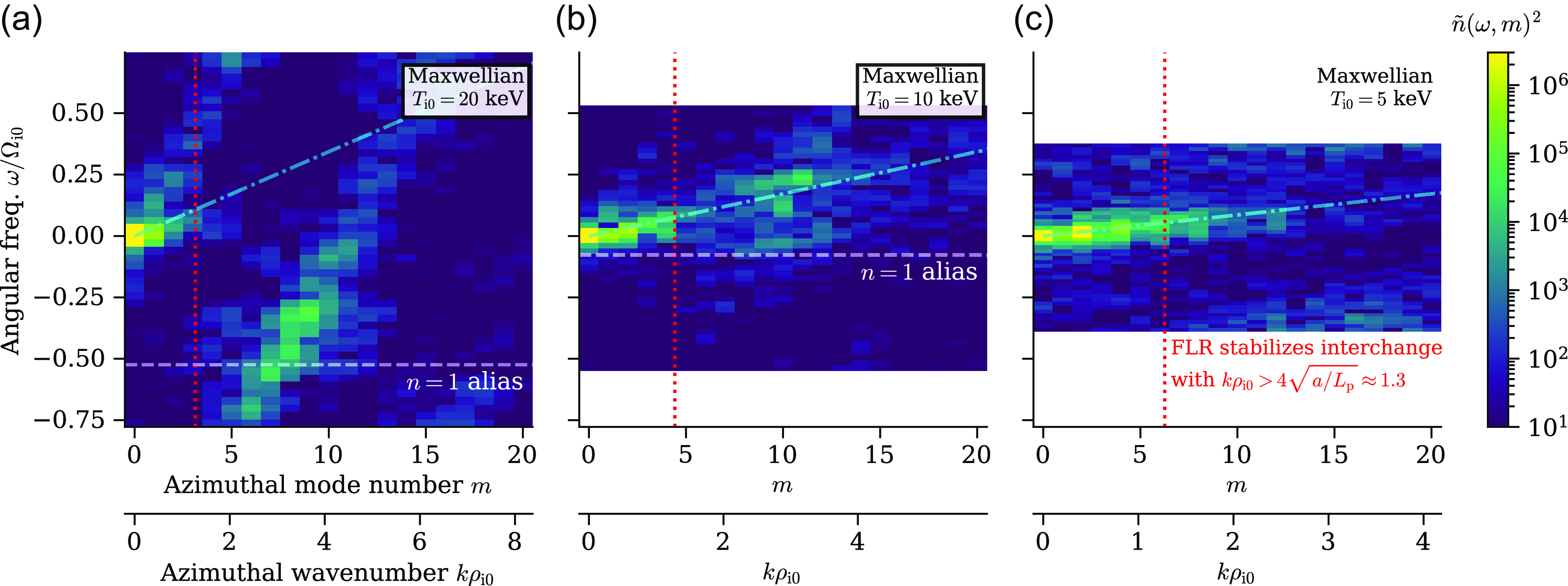
Figure 13. Interchange modes appear and DCLC weakens as $T_{{i}}$
decreases (a to c) in simulations of Maxwellian ions in WHAM’s
$T_{{i}}$
decreases (a to c) in simulations of Maxwellian ions in WHAM’s $R_{{m}}=20$
magnetic-field geometry. Fourier spectra computed as in figure 6. The dot–dashed cyan line plots the interchange mode’s expected phase velocity,
$R_{{m}}=20$
magnetic-field geometry. Fourier spectra computed as in figure 6. The dot–dashed cyan line plots the interchange mode’s expected phase velocity, $\omega /k = v_{\mathrm{Di}}/2$
, assuming spatial gradient
$\omega /k = v_{\mathrm{Di}}/2$
, assuming spatial gradient $\epsilon = (10 \;\mathrm{cm})^{-1}$
.
$\epsilon = (10 \;\mathrm{cm})^{-1}$
.
Alfvén ion cyclotron (AIC) modes do not appear at significant amplitude in our simulations; recall that both $\delta B_r$
and
$\delta B_r$
and $\delta B_\theta$
are small (§ 3.1), and pitch-angle scattering is weak compared with DCLC’s
$\delta B_\theta$
are small (§ 3.1), and pitch-angle scattering is weak compared with DCLC’s $v_\perp$
scattering (figure 3). Does our non-observation agree with theory and prior experiments? An empirical criterion for AIC growth, obtained from experiments on the tandem mirror GAMMA-10 (Ichimura et al. Reference Ichimura, Inutake, Katsumata, Hino, Hojo, Ishii, Tamano and Miyoshi1993; Katsumata et al. Reference Katsumata, Ichimura, Inutake, Hojo, Mase and Tamano1996), is
$v_\perp$
scattering (figure 3). Does our non-observation agree with theory and prior experiments? An empirical criterion for AIC growth, obtained from experiments on the tandem mirror GAMMA-10 (Ichimura et al. Reference Ichimura, Inutake, Katsumata, Hino, Hojo, Ishii, Tamano and Miyoshi1993; Katsumata et al. Reference Katsumata, Ichimura, Inutake, Hojo, Mase and Tamano1996), is
 \begin{equation} T_{{i}\perp }/T_{{i}\parallel } \gt 0.55/\beta _{\perp }^{0.5} ,\end{equation}
based on data with $\beta _\perp \lt 0.03$
. One linear-instability criterion, derived for a homogeneous bi-Maxwellian plasma (Gary et al. Reference Gary, McKean, Winske, Anderson, Denton and Fuselier1994) and with a form commonly used in the solar-wind literature (e.g. Hellinger et al. Reference Hellinger, Trávníček, Kasper and Lazarus2006), is
$\beta _\perp \lt 0.03$
. One linear-instability criterion, derived for a homogeneous bi-Maxwellian plasma (Gary et al. Reference Gary, McKean, Winske, Anderson, Denton and Fuselier1994) and with a form commonly used in the solar-wind literature (e.g. Hellinger et al. Reference Hellinger, Trávníček, Kasper and Lazarus2006), is
 \begin{equation} T_{{i}\perp }/T_{{i}\parallel } \gt 1 + 0.43/\beta _{\parallel }^{0.42} .\end{equation}
At $t=0$
in our
$t=0$
in our $R_{{m}}=20$
simulation, the sloshing-ion turning points have
$R_{{m}}=20$
simulation, the sloshing-ion turning points have $\beta _{\perp } = 8\pi n T_{{i}\perp } / B^2 = 0.17$
and
$\beta _{\perp } = 8\pi n T_{{i}\perp } / B^2 = 0.17$
and $\beta _{\parallel } = 8\pi n T_{{i}\parallel } / B^2 = 0.068$
, with corresponding anisotropy
$\beta _{\parallel } = 8\pi n T_{{i}\parallel } / B^2 = 0.068$
, with corresponding anisotropy $T_{{i}\perp }/T_{{i}\parallel } = 2.5$
; our simulations with larger
$T_{{i}\perp }/T_{{i}\parallel } = 2.5$
; our simulations with larger $R_{{m}}$
have similar anisotropy and lower plasma beta at the turning points. Both (4.6) and (4.7) indicate that AIC may be unstable at the turning points.
$R_{{m}}$
have similar anisotropy and lower plasma beta at the turning points. Both (4.6) and (4.7) indicate that AIC may be unstable at the turning points.
So, why does AIC not appear? First, since AIC is driven by gradients of $f$
on resonant surfaces in velocity space, (4.6) and (4.7) will not be so precise when applied to different ion distributions; for example, Isenberg et al. (Reference Isenberg, Maruca and Kasper2013) noted that subtle modifications to
$f$
on resonant surfaces in velocity space, (4.6) and (4.7) will not be so precise when applied to different ion distributions; for example, Isenberg et al. (Reference Isenberg, Maruca and Kasper2013) noted that subtle modifications to $f$
at marginal AIC stability can modify anisotropy thresholds based on bi-Maxwellian temperatures by a factor of
$f$
at marginal AIC stability can modify anisotropy thresholds based on bi-Maxwellian temperatures by a factor of $\mathord {\sim } 2$
. Second, AIC is stabilized by the inhomogeneous plasma in WHAM. Sloshing ions put perpendicular pressure anisotropy at turning points, so instability drive weakens towards the mirror cell’s centre. A small plasma column radius with respect to the ion Larmor radius also aids stability (Tsidulko & Chernoshtanov Reference Tsidulko and Chernoshtanov2014). And, AIC is suppressed if the mirror’s axial length is shorter than a critical length (Tajima et al. Reference Tajima, Mima and Dawson1977; Tajima & Mima Reference Tajima and Mima1980; Nicks et al. Reference Nicks, Putvinski and Tajima2023),
$\mathord {\sim } 2$
. Second, AIC is stabilized by the inhomogeneous plasma in WHAM. Sloshing ions put perpendicular pressure anisotropy at turning points, so instability drive weakens towards the mirror cell’s centre. A small plasma column radius with respect to the ion Larmor radius also aids stability (Tsidulko & Chernoshtanov Reference Tsidulko and Chernoshtanov2014). And, AIC is suppressed if the mirror’s axial length is shorter than a critical length (Tajima et al. Reference Tajima, Mima and Dawson1977; Tajima & Mima Reference Tajima and Mima1980; Nicks et al. Reference Nicks, Putvinski and Tajima2023),
 \begin{equation} L_{\mathrm{c}} = 2 \pi ^2 \sqrt { \frac {T_{{i}\parallel }}{\beta _\perp T_{{i}\perp }} } \left ( \frac {c}{\omega _{\mathrm{pi}}} \right ) .\end{equation}
The critical length $L_{\mathrm{c}} \approx 182 \;\mathrm{cm}$
is very close to WHAM’s length
$L_{\mathrm{c}} \approx 182 \;\mathrm{cm}$
is very close to WHAM’s length $2 L_{\mathrm{p}} = 196 \;\mathrm{cm}$
, again taking
$2 L_{\mathrm{p}} = 196 \;\mathrm{cm}$
, again taking $\beta _\perp = 0.17$
and assuming
$\beta _\perp = 0.17$
and assuming $c/\omega _{\mathrm{pi}}=5.9\;\mathrm{cm}$
for density
$c/\omega _{\mathrm{pi}}=5.9\;\mathrm{cm}$
for density $n = 3 \times 10^{13} \;\mathrm{cm^{-3}}$
at sloshing-ion turning points. Third, DCLC simply has a faster growth rate and decreases plasma beta before AIC can be triggered.
$n = 3 \times 10^{13} \;\mathrm{cm^{-3}}$
at sloshing-ion turning points. Third, DCLC simply has a faster growth rate and decreases plasma beta before AIC can be triggered.
To summarize: AIC with low axial mode number may be marginally unstable for WHAM, based on the highest possible $\beta _{\perp }$
and density
$\beta _{\perp }$
and density $n$
at sloshing-ion turning points. But multiple effects weaken AIC drive and so may explain why it does not appear in our simulations.
$n$
at sloshing-ion turning points. But multiple effects weaken AIC drive and so may explain why it does not appear in our simulations.
4.5. Comparison with real mirrors
In real mirror devices, discrete DCLC modes can persist stably for $\mathord {\sim } {\mathcal{O}}(1 \;\mathrm{ms})$
(Shmigelsky et al. Reference Shmigelsky, Meyster, Chernoshtanov, Lizunov, Solomakhin and Yakovlev2024), but DCLC can also appear as discrete bursts of enhanced fluctuations with duration
$\mathord {\sim } {\mathcal{O}}(1 \;\mathrm{ms})$
(Shmigelsky et al. Reference Shmigelsky, Meyster, Chernoshtanov, Lizunov, Solomakhin and Yakovlev2024), but DCLC can also appear as discrete bursts of enhanced fluctuations with duration $\mathord {\sim } 10$
to
$\mathord {\sim } 10$
to $100 \;\mathrm{\unicode{x03BC}s}$
(Coensgen et al. Reference Coensgen, Cummins, Logan, Molvik, Nexsen, Simonen, Stallard and Turner1975; Yamaguchi Reference Yamaguchi1996; Shmigelsky et al. Reference Shmigelsky, Meyster, Chernoshtanov, Lizunov, Solomakhin and Yakovlev2024). Our simulations do not show bursting, nor did previous simulations by Cohen et al. (Reference Cohen, Smith, Maron and Nevins1983). Yamaguchi (Reference Yamaguchi1996) explained bursting DCLC in the GAMMA-6A experiment using a quasilinear model with bounce-averaged electron Landau damping; they appealed to (i) separation between DCLC scattering and axial outflow time scales (i.e.
$100 \;\mathrm{\unicode{x03BC}s}$
(Coensgen et al. Reference Coensgen, Cummins, Logan, Molvik, Nexsen, Simonen, Stallard and Turner1975; Yamaguchi Reference Yamaguchi1996; Shmigelsky et al. Reference Shmigelsky, Meyster, Chernoshtanov, Lizunov, Solomakhin and Yakovlev2024). Our simulations do not show bursting, nor did previous simulations by Cohen et al. (Reference Cohen, Smith, Maron and Nevins1983). Yamaguchi (Reference Yamaguchi1996) explained bursting DCLC in the GAMMA-6A experiment using a quasilinear model with bounce-averaged electron Landau damping; they appealed to (i) separation between DCLC scattering and axial outflow time scales (i.e. $1/\nu _{\perp \perp } \ll \tau _{\mathrm{GD}}$
); and (ii) fast time variation in DCLC growth rate with slower variation in electron-Landau damping rate. In our simulations,
$1/\nu _{\perp \perp } \ll \tau _{\mathrm{GD}}$
); and (ii) fast time variation in DCLC growth rate with slower variation in electron-Landau damping rate. In our simulations, $1/\nu _{\perp \perp } \sim \tau _{\mathrm{GD}}$
at order of magnitude (figure 8
b); DCLC appears marginally stable and does not damp upon ions within a time scale
$1/\nu _{\perp \perp } \sim \tau _{\mathrm{GD}}$
at order of magnitude (figure 8
b); DCLC appears marginally stable and does not damp upon ions within a time scale $\ll \tau _{\mathrm{GD}}$
. It would be interesting to see if future kinetic simulations with longer simulation durations, electron-Landau damping or other physical effects can replicate DCLC bursting.
$\ll \tau _{\mathrm{GD}}$
. It would be interesting to see if future kinetic simulations with longer simulation durations, electron-Landau damping or other physical effects can replicate DCLC bursting.
Both TMX-U and GDT saw that DCLC could be driven at sloshing-ion turning points instead of at the mirror midplane $z=0$
(Berzins & Casper Reference Berzins and Casper1987; Shmigelsky et al. Reference Shmigelsky, Meyster, Chernoshtanov, Lizunov, Solomakhin and Yakovlev2024). Why does DCLC have strongest drive at
$z=0$
(Berzins & Casper Reference Berzins and Casper1987; Shmigelsky et al. Reference Shmigelsky, Meyster, Chernoshtanov, Lizunov, Solomakhin and Yakovlev2024). Why does DCLC have strongest drive at $z=0$
, versus at the turning points, in our simulations of WHAM? In TMX-U, the end-plug could be stabilized on one side and not the other due to a combination of axial flows from the central cell and localized ECH at the end-plug outer-turning point (Berzins & Casper Reference Berzins and Casper1987). As for GDT versus WHAM, we cannot answer definitively, but we note that WHAM’s shorter axial length of
$z=0$
, versus at the turning points, in our simulations of WHAM? In TMX-U, the end-plug could be stabilized on one side and not the other due to a combination of axial flows from the central cell and localized ECH at the end-plug outer-turning point (Berzins & Casper Reference Berzins and Casper1987). As for GDT versus WHAM, we cannot answer definitively, but we note that WHAM’s shorter axial length of $2\;\mathrm{m}$
may constrain DCLC’s axial eigenmodes as compared with GDT’s
$2\;\mathrm{m}$
may constrain DCLC’s axial eigenmodes as compared with GDT’s $7 \;\mathrm{m}$
length.
$7 \;\mathrm{m}$
length.
Where do cool ions come from in real experiments? In WHAM, DCLC-scattered ions escape with large $|v_\parallel |$
and are not trapped. Charge exchange between beam ions and cool neutrals can generate
$|v_\parallel |$
and are not trapped. Charge exchange between beam ions and cool neutrals can generate $\lt 1 \;\mathrm{keV}$
ions that trap in the midplane’s electrostatic potential well; prerequisite cool neutrals naturally outgas from plasma-facing materials. In tandem mirrors like TMX-U, central-cell outflow into end-plug cells can also provide cool ions to stabilize DCLC (Simonen et al. Reference Simonen1983; Berzins & Casper Reference Berzins and Casper1987). Central-cell outflow may also help to reduce the growth rate of curvature-driven collisionless trapped-particle modes (Rosenbluth Reference Rosenbluth1982; Berk et al. Reference Berk, Rosenbluth, Wong, Antonsen and Baldwin1983), as outflowing ions can sample good curvature near mirror throats and help to couple adjacent MHD-unstable and stable mirror cells.
$\lt 1 \;\mathrm{keV}$
ions that trap in the midplane’s electrostatic potential well; prerequisite cool neutrals naturally outgas from plasma-facing materials. In tandem mirrors like TMX-U, central-cell outflow into end-plug cells can also provide cool ions to stabilize DCLC (Simonen et al. Reference Simonen1983; Berzins & Casper Reference Berzins and Casper1987). Central-cell outflow may also help to reduce the growth rate of curvature-driven collisionless trapped-particle modes (Rosenbluth Reference Rosenbluth1982; Berk et al. Reference Berk, Rosenbluth, Wong, Antonsen and Baldwin1983), as outflowing ions can sample good curvature near mirror throats and help to couple adjacent MHD-unstable and stable mirror cells.
Cool-ion stabilization of DCLC may face problems in larger and more powerful mirrors. The axial electrostatic well at $z=0$
, which traps cool ions, will become shallower due to ion–ion pitch-angle scattering of the beam ions. Pitch-angle scattering is counter-balanced by neutral-beam capture via charge exchange (CX) or impact ionization, as both processes create new hot ions with
$z=0$
, which traps cool ions, will become shallower due to ion–ion pitch-angle scattering of the beam ions. Pitch-angle scattering is counter-balanced by neutral-beam capture via charge exchange (CX) or impact ionization, as both processes create new hot ions with $45^\circ$
pitch-angle. The CX between hot ions / fast neutrals also pumps out the isotropized, scattered hot ions, so one CX event collimates the ions’ pitch-angle distribution more effectively than one impact-ionization event. But, the CX cross-section drops relative to impact ionization for beam energies
$45^\circ$
pitch-angle. The CX between hot ions / fast neutrals also pumps out the isotropized, scattered hot ions, so one CX event collimates the ions’ pitch-angle distribution more effectively than one impact-ionization event. But, the CX cross-section drops relative to impact ionization for beam energies $\gtrsim 70 \;\mathrm{keV}$
(Endrizzi et al. Reference Endrizzi2023, figure 10). It thus becomes harder to collimate the ion pitch-angle distribution and harder to maintain an axial electrostatic potential well with
$\gtrsim 70 \;\mathrm{keV}$
(Endrizzi et al. Reference Endrizzi2023, figure 10). It thus becomes harder to collimate the ion pitch-angle distribution and harder to maintain an axial electrostatic potential well with ${\mathcal{O}}(10^2) \;\mathrm{keV}$
NBI (e.g. Forest et al. Reference Forest2024, figure 6). And, tandem central-cell outflow reduces fusion performance and may set limits on power-plant reactor design (e.g. Frank et al. Reference Frank2025, § 3.2). Future mirror designs may thus need other methods to help stabilize DCLC.
${\mathcal{O}}(10^2) \;\mathrm{keV}$
NBI (e.g. Forest et al. Reference Forest2024, figure 6). And, tandem central-cell outflow reduces fusion performance and may set limits on power-plant reactor design (e.g. Frank et al. Reference Frank2025, § 3.2). Future mirror designs may thus need other methods to help stabilize DCLC.
The WHAM experiment began operating in July 2024 (Anderson et al. Reference Anderson2024). A comparison between experimental data and our simulations is not yet available. We anticipate that WHAM plasmas and diagnostics may be tuned to create and measure DCLC modes in future experimental campaigns.
5. Conclusions
We have performed 3-D kinetic-ion simulations of WHAM, initialized with a neutral-beam-injected deuteron population with $T_{{i}} \sim 10 \;\mathrm{keV}$
and cool, isothermal-fluid electrons with
$T_{{i}} \sim 10 \;\mathrm{keV}$
and cool, isothermal-fluid electrons with $T_{{e}} \sim 1 \;\mathrm{keV}$
, to assess kinetic plasma stability in a high-performance, collisionless-ion regime. We find that WHAM’s beam-ion distribution is unstable to an electrostatic, flute-like (
$T_{{e}} \sim 1 \;\mathrm{keV}$
, to assess kinetic plasma stability in a high-performance, collisionless-ion regime. We find that WHAM’s beam-ion distribution is unstable to an electrostatic, flute-like ( $k \approx k_\perp$
) mode that grows on
$k \approx k_\perp$
) mode that grows on $\lesssim 1 \;\mathrm{\unicode{x03BC}s}$
time scales; it propagates azimuthally around the column in the ion diamagnetic direction and has angular frequency between
$\lesssim 1 \;\mathrm{\unicode{x03BC}s}$
time scales; it propagates azimuthally around the column in the ion diamagnetic direction and has angular frequency between $\Omega _{\mathrm{i0}}$
and
$\Omega _{\mathrm{i0}}$
and $2\Omega _{\mathrm{i0}}$
. We identify it as the DCLC mode, well known from prior mirror experiments (Coensgen et al. Reference Coensgen, Cummins, Logan, Molvik, Nexsen, Simonen, Stallard and Turner1975) and previously anticipated to be a possible concern for WHAM (Endrizzi et al. Reference Endrizzi2023).
$2\Omega _{\mathrm{i0}}$
. We identify it as the DCLC mode, well known from prior mirror experiments (Coensgen et al. Reference Coensgen, Cummins, Logan, Molvik, Nexsen, Simonen, Stallard and Turner1975) and previously anticipated to be a possible concern for WHAM (Endrizzi et al. Reference Endrizzi2023).
The plasma column and DCLC fluctuations settle into a steady-state decay by $t = 6 \;\mathrm{\unicode{x03BC}s}$
. Particles escape axially with confinement time
$t = 6 \;\mathrm{\unicode{x03BC}s}$
. Particles escape axially with confinement time $\tau _{\mathrm{p}} = n / (\mathrm{d} n/\mathrm{d} t) \sim 10^2 \;\mathrm{\unicode{x03BC}s}$
in a ‘gas dynamic’ regime, wherein the scattering rate into the loss cone equals or exceeds the rate of free-streaming axial loss from the mirror. Particle losses are due to collisionless
$\tau _{\mathrm{p}} = n / (\mathrm{d} n/\mathrm{d} t) \sim 10^2 \;\mathrm{\unicode{x03BC}s}$
in a ‘gas dynamic’ regime, wherein the scattering rate into the loss cone equals or exceeds the rate of free-streaming axial loss from the mirror. Particle losses are due to collisionless $v_\perp$
scattering upon the DCLC modes; the particle–wave correlation time is approximately
$v_\perp$
scattering upon the DCLC modes; the particle–wave correlation time is approximately ${\Omega _{\mathrm{i0}}}^{-1}$
at the mirror midplane. Particle losses and velocity-space diffusion are strongest at the plasma’s radial edge, whereas the plasma column’s core can maintain
${\Omega _{\mathrm{i0}}}^{-1}$
at the mirror midplane. Particle losses and velocity-space diffusion are strongest at the plasma’s radial edge, whereas the plasma column’s core can maintain $\mathrm{d} F/\mathrm{d} v_\perp \gt 0$
at low
$\mathrm{d} F/\mathrm{d} v_\perp \gt 0$
at low $v_\perp$
.
$v_\perp$
.
We review well known and experimentally tested methods for stabilizing DCLC: addition of cool plasma to fill the loss cone, larger plasma extent (smaller gradient) and parallel electron kinetics including Landau damping. In 3-D simulations with cool ions initialized at the plasma’s radial edge, the beam ions’ confinement time can be raised by up to $9\times$
, though an order-unity ratio of cool/hot ion number density is needed and the cool-ion confinement is poorer than that of the beam ions. The best-case beam-ion confinement time of several
$9\times$
, though an order-unity ratio of cool/hot ion number density is needed and the cool-ion confinement is poorer than that of the beam ions. The best-case beam-ion confinement time of several $100 \;\mathrm{\unicode{x03BC}s}$
also remains two orders of magnitude below the ideal, ‘classical’ confinement time of 0.1–0.2 s. In a real experiment, the cool ions must be provided and replenished by external sources because DCLC does not scatter beam ions into the axial electrostatic potential well (Kesner Reference Kesner1973, Reference Kesner1980) where they could be trapped to help stabilize DCLC. The DCLC-scattered beam ions are lost because they retain large parallel speeds and so never enter the trapped region of phase space.
$100 \;\mathrm{\unicode{x03BC}s}$
also remains two orders of magnitude below the ideal, ‘classical’ confinement time of 0.1–0.2 s. In a real experiment, the cool ions must be provided and replenished by external sources because DCLC does not scatter beam ions into the axial electrostatic potential well (Kesner Reference Kesner1973, Reference Kesner1980) where they could be trapped to help stabilize DCLC. The DCLC-scattered beam ions are lost because they retain large parallel speeds and so never enter the trapped region of phase space.
Our simulations are limited, especially in the electric field model and isothermal-fluid electron closure. Future work may incorporate electron inertia, an electron energy equation, drift-kinetic electrons or more to help model (i) bounce-averaged electron Landau damping, and (ii) the plasma’s axial and radial electric potential structure, which dictate outflows and rotation. And, the initial condition of a hot, beam-ion plasma with only mild slowing-down upon electrons is idealized. A two-way coupling between Hybrid-VPIC and CQL3D-m over a $20\;\mathrm{ms}$
laboratory shot duration, passing DCLC quasilinear diffusion coefficients from kinetic simulations into the Fokker–Planck equation, may yield more realistic predictions. Adding neutral-ion interactions to our CQL3D-m models would improve our cool-ion stabilization modelling. Other subsystems on WHAM are not modelled, for example heating of ions and electrons via radio-frequency and microwave radiation, respectively, or biased end-rings within the expanders used to drive rotation and shear flow. So, future work may also consider a wider range of fuelling and heating scenarios in WHAM and next-step mirror devices.
$20\;\mathrm{ms}$
laboratory shot duration, passing DCLC quasilinear diffusion coefficients from kinetic simulations into the Fokker–Planck equation, may yield more realistic predictions. Adding neutral-ion interactions to our CQL3D-m models would improve our cool-ion stabilization modelling. Other subsystems on WHAM are not modelled, for example heating of ions and electrons via radio-frequency and microwave radiation, respectively, or biased end-rings within the expanders used to drive rotation and shear flow. So, future work may also consider a wider range of fuelling and heating scenarios in WHAM and next-step mirror devices.
Supplementary material
The supplementary material for this article can be found at https://doi.org/10.1017/S0022377825000480
Acknowledgements
Conversations with D. Bindl, S. Dettrick, M. Francisquez, R. Groenewald, M. Koepke, D. Ryutov, D. Sutherland, D. Yakovlev, M. Yu and the entire WHAM team are gratefully acknowledged. We also thank the anonymous referees for constructive comments that have improved this paper.
Editor Peter Catto thanks the referees for their advice in evaluating this article.
Funding
Funding for this work was provided by Realta Fusion, the U.S. Department of Energy (DOE), and the U.S. National Science Foundation (NSF). WHAM collaboration work is supported by the U.S. DOE through ARPA-E DE-AR0001258, Commonwealth Fusion Systems, Realta Fusion, Wisconsin Alumni Research Foundation and a lengthy list of collaborators providing valuable equipment. AT was partly supported by NSF PHY-2010189 and the DOE Fusion Energy Sciences Postdoctoral Research Program, administered by the Oak Ridge Institute for Science and Education (ORISE) and Oak Ridge Associated Universities (ORAU) under DOE contract DE-SC0014664.
High-performance computing resources were provided by the National Energy Research Scientific Computing Center (NERSC), a DOE Office of Science User Facility, via allocation FES-ERCAP0026655; Anvil at Purdue University’s Rosen Center for Advanced Computing (McCartney et al. Reference McCartney, Hacker and Yang2014; Song et al. Reference Song2022) via allocation PHY230179 from the NSF Advanced Cyberinfrastructure Coordination Ecosystem: Services & Support (ACCESS) program; Amazon Web Services’ Compute for Climate Fellowship awarded to Realta Fusion; Los Alamos Institutional Computing; and UW–Madison’s Center for High Throughput Computing (Center for High Throughput Computing, 2006). ACCESS (Boerner et al. Reference Boerner, Deems, Furlani, Knuth and Towns2023) is supported by NSF grants #2138259, #2138286, #2138307, #2137603 and #2138296.
All opinions expressed in this paper are the authors’ and do not necessarily reflect the policies and views of DOE, ORAU or ORISE.
Declaration of interests
C.B.F. is a co-founder of Realta Fusion; D.A.E., S.J.F. and J.V. are employees of Realta Fusion. This work was partly supported by a grant from Realta Fusion to the University of Wisconsin–Madison.
Appendix A. Hyper-resistivity scan
Hyper-resistivity, although intended to suppress gridscale numerical noise, may also alter DCLC mode structure as discussed in § 2.2. Figure 14 shows that raising or decreasing $\eta _{{H}}$
by a factor of
$\eta _{{H}}$
by a factor of $3$
alters the spectrum of density fluctuations at the plasma edge; with higher
$3$
alters the spectrum of density fluctuations at the plasma edge; with higher $\eta _{{H}}$
, the spectrum broadens and is less coherent.
$\eta _{{H}}$
, the spectrum broadens and is less coherent.
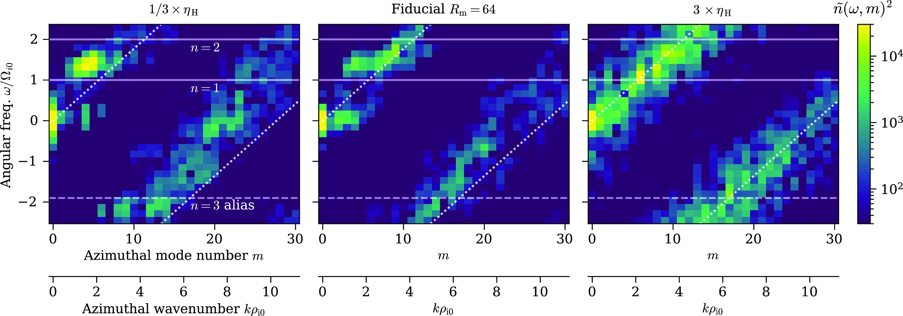
Figure 14. Effect of hyper-resistivity, increasing (a) to (c), upon density-fluctuation Fourier spectra in WHAM $R_{{m}}=64$
simulations; panel (b) is the same data as figure 6(c). Fourier spectra and annotations constructed like in figure 6, at same
$R_{{m}}=64$
simulations; panel (b) is the same data as figure 6(c). Fourier spectra and annotations constructed like in figure 6, at same $r=2.69\rho _{\mathrm{i0}}$
over
$r=2.69\rho _{\mathrm{i0}}$
over $t=3$
to
$t=3$
to $6\,\tau _{\mathrm{bounce}}$
, but the colourmap range and 2-D plot domain/range are changed.
$6\,\tau _{\mathrm{bounce}}$
, but the colourmap range and 2-D plot domain/range are changed.
Appendix B. Electron parallel response
To obtain the electrons’ parallel response in § 4.3, we start again from Stix (Reference Stix1992, § 14-3, (9)), neglecting spatial derivatives of order $\partial ^2 g/\partial y^2$
or higher in Stix’s notation, where
$\partial ^2 g/\partial y^2$
or higher in Stix’s notation, where $g$
is the guiding-centre distribution. For a Maxwellian guiding-centre distribution, the susceptibility is
$g$
is the guiding-centre distribution. For a Maxwellian guiding-centre distribution, the susceptibility is
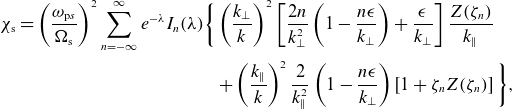 \begin{align} \chi _{\mathrm{s}} = \left (\frac {\omega _{\mathrm{p}s}}{\Omega _{\mathrm{s}}}\right )^2 \sum _{n=-\infty }^{\infty } e^{-\lambda } I_n(\lambda ) \bigg \{ &\left (\frac {k_\perp }{k}\right )^2 \left [ \frac {2 n}{k_\perp ^2} \left ( 1 - \frac {n \epsilon }{k_\perp } \right ) + \frac {\epsilon }{k_\perp } \right ] \frac {Z(\zeta _n)}{k_\parallel } \nonumber \\ & + \left (\frac {k_\parallel }{k}\right )^2 \frac {2}{k_\parallel ^2} \left ( 1 - \frac {n \epsilon }{k_\perp } \right ) \left [ 1 + \zeta _n Z(\zeta _n) \right ] \bigg \} ,\end{align}
where the modified Bessel function $I_n(\lambda )$
has argument
$I_n(\lambda )$
has argument $\lambda = k_\perp ^2/2$
, the plasma dispersion function
$\lambda = k_\perp ^2/2$
, the plasma dispersion function $Z(\zeta _n)$
has argument
$Z(\zeta _n)$
has argument $\zeta _n = (\omega -n)/k_\parallel$
and the variables
$\zeta _n = (\omega -n)/k_\parallel$
and the variables $\omega , \epsilon , k, k_\perp , k_\parallel$
are all dimensionless following the same species-specific scheme used for (3.3). Equation (B1) is valid for any
$\omega , \epsilon , k, k_\perp , k_\parallel$
are all dimensionless following the same species-specific scheme used for (3.3). Equation (B1) is valid for any $\boldsymbol{k}$
angle. The limit
$\boldsymbol{k}$
angle. The limit $\zeta _n \to \infty$
and
$\zeta _n \to \infty$
and $k_\parallel /k \to 0$
recovers the perpendicular susceptibility given by (3.3). The limit
$k_\parallel /k \to 0$
recovers the perpendicular susceptibility given by (3.3). The limit $\epsilon /k_\perp \to 0$
recovers the standard Harris (Reference Harris1959) dispersion relation (Gurnett & Bhattacharjee Reference Gurnett and Bhattacharjee2017, § 10.2).
$\epsilon /k_\perp \to 0$
recovers the standard Harris (Reference Harris1959) dispersion relation (Gurnett & Bhattacharjee Reference Gurnett and Bhattacharjee2017, § 10.2).
Let us simplify (B1). Take the limits $\lambda \to 0$
and
$\lambda \to 0$
and $\zeta _{\pm 1} = (\omega \mp 1)/k_\parallel \approx \mp 1/k_\parallel \to \infty$
in order to expand
$\zeta _{\pm 1} = (\omega \mp 1)/k_\parallel \approx \mp 1/k_\parallel \to \infty$
in order to expand $e^{-\lambda } I_n(\lambda )$
and
$e^{-\lambda } I_n(\lambda )$
and $Z(\zeta _{\pm 1})$
. But, make no assumptions on the magnitude of
$Z(\zeta _{\pm 1})$
. But, make no assumptions on the magnitude of $\zeta _0 = \omega /k_\parallel$
. Also, drop all
$\zeta _0 = \omega /k_\parallel$
. Also, drop all $|n| \gt 1$
Bessel terms. The result is
$|n| \gt 1$
Bessel terms. The result is
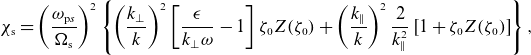 \begin{equation} \chi _{\mathrm{s}} = \left (\frac {\omega _{\mathrm{p}s}}{\Omega _{\mathrm{s}}}\right )^2 \left \{ \left (\frac {k_\perp }{k}\right )^2 \left [ \frac {\epsilon }{k_\perp \omega } - 1 \right ] \zeta _0 Z(\zeta _0) + \left (\frac {k_\parallel }{k}\right )^2 \frac {2}{k_\parallel ^2} \left [ 1 + \zeta _0 Z(\zeta _0) \right ] \right \} ,\end{equation}
which yields (4.4) after putting in dimensions. The limit $\zeta _0 \to \infty$
recovers the familiar cold-fluid result, written as follows in dimensional variables:
$\zeta _0 \to \infty$
recovers the familiar cold-fluid result, written as follows in dimensional variables:
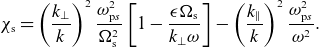 \begin{equation} \chi _{\mathrm{s}} = \left (\frac {k_\perp }{k}\right )^2 \frac {\omega _{\mathrm{p}s}^2}{\Omega _{\mathrm{s}}^2} \left [ 1 - \frac {\epsilon \Omega _{\mathrm{s}}}{k_\perp \omega } \right ] - \left (\frac {k_\parallel }{k}\right )^2 \frac {\omega _{\mathrm{p}s}^2}{\omega ^2} .\end{equation}
A subtlety appears when expanding (B1) into (B2). Consider the susceptibility tensor components $\chi _{\perp \perp }$
and
$\chi _{\perp \perp }$
and $\chi _{\parallel \parallel }$
for a hot homogeneous plasma (Stix Reference Stix1992, § 10). The perpendicular response simplifies in the cold-fluid limit,
$\chi _{\parallel \parallel }$
for a hot homogeneous plasma (Stix Reference Stix1992, § 10). The perpendicular response simplifies in the cold-fluid limit,
 \begin{equation} \chi _{\perp \perp } \to \frac {\omega _{\mathrm{p}s}^2}{\Omega _{\mathrm{s}}^2} .\end{equation}
But, $\chi _{\perp \perp }$
is cancelled by the analogous expansion of
$\chi _{\perp \perp }$
is cancelled by the analogous expansion of $\chi _{\parallel \parallel }$
when (i) both
$\chi _{\parallel \parallel }$
when (i) both $k_\perp$
and
$k_\perp$
and $k_\parallel$
are finite; (ii)
$k_\parallel$
are finite; (ii) $\zeta _0$
is kept finite; and (iii) terms of order
$\zeta _0$
is kept finite; and (iii) terms of order $\mathcal{O}(\lambda ^1)$
are kept in expanding
$\mathcal{O}(\lambda ^1)$
are kept in expanding $e^{-\lambda } I_0(\lambda )$
. The said expansion gives
$e^{-\lambda } I_0(\lambda )$
. The said expansion gives
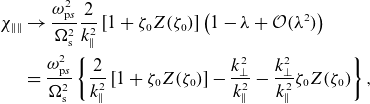 \begin{align} \chi _{\parallel \parallel } &\to \frac {\omega _{\mathrm{p}s}^2}{\Omega _{\mathrm{s}}^2} \frac {2}{k_\parallel ^2} \left [ 1 + \zeta _0 Z(\zeta _0) \right ] \left ( 1 - \lambda + \mathcal{O}(\lambda ^2) \right ) \nonumber \\ &= \frac {\omega _{\mathrm{p}s}^2}{\Omega _{\mathrm{s}}^2} \left \{ \frac {2}{k_\parallel ^2} \left [ 1 + \zeta _0 Z(\zeta _0) \right ] - \frac {k_\perp ^2}{k_\parallel ^2} - \frac {k_\perp ^2}{k_\parallel ^2} \zeta _0 Z(\zeta _0) \right \} ,\end{align}
with $k_\parallel$
dimensionless as before. Then, in the combined electrostatic susceptibility
$k_\parallel$
dimensionless as before. Then, in the combined electrostatic susceptibility
 \begin{equation} \chi \approx (k_\perp /k)^2 \chi _{\perp \perp } + (k_\parallel /k)^2 \chi _{\parallel \parallel } + (2 k_\parallel k_\perp /k^2) \chi _{\perp \parallel } ,\end{equation}
we see that (B4) and (B5) partly cancel, and only a parallel contribution $-(k_\perp /k)^2 (\omega _{\mathrm{p}s}/\Omega _{\mathrm{s}})^2 \zeta _0 Z(\zeta _0)$
remains. This remainder term can be seen in (B2). When the
$-(k_\perp /k)^2 (\omega _{\mathrm{p}s}/\Omega _{\mathrm{s}})^2 \zeta _0 Z(\zeta _0)$
remains. This remainder term can be seen in (B2). When the $\zeta _0 \to \infty$
limit is taken, it is this parallel remainder that provides the usual perpendicular response
$\zeta _0 \to \infty$
limit is taken, it is this parallel remainder that provides the usual perpendicular response $\chi _{\perp \perp } \to \omega _{\mathrm{p}s}^2/\Omega _{\mathrm{s}}^2$
. This is to some extent a semantic quibble; we can also say that the remainder term
$\chi _{\perp \perp } \to \omega _{\mathrm{p}s}^2/\Omega _{\mathrm{s}}^2$
. This is to some extent a semantic quibble; we can also say that the remainder term $-(k_\perp /k)^2 (\omega _{\mathrm{p}s}/\Omega _{\mathrm{s}})^2 \zeta _0 Z(\zeta _0)$
cancels the parallel term
$-(k_\perp /k)^2 (\omega _{\mathrm{p}s}/\Omega _{\mathrm{s}})^2 \zeta _0 Z(\zeta _0)$
cancels the parallel term $-(k_\perp /k)^2 (\omega _{\mathrm{p}s}/\Omega _{\mathrm{s}})^2$
to leave only the perpendicular term
$-(k_\perp /k)^2 (\omega _{\mathrm{p}s}/\Omega _{\mathrm{s}})^2$
to leave only the perpendicular term $ + (k_\perp /k)^2 (\omega _{\mathrm{p}s}/\Omega _{\mathrm{s}})^2$
in (B6). But, the overall point stands that the perpendicular term in (B2) can be significantly modified by the parallel response, even when
$ + (k_\perp /k)^2 (\omega _{\mathrm{p}s}/\Omega _{\mathrm{s}})^2$
in (B6). But, the overall point stands that the perpendicular term in (B2) can be significantly modified by the parallel response, even when $k_\parallel \ll k_\perp$
; the regulating parameter is
$k_\parallel \ll k_\perp$
; the regulating parameter is $\zeta _0$
.
$\zeta _0$
.


 Open access