


1. Introduction
Gyrokinetics is a mean-field theory which is used, among other things, to investigate transport phenomena in magnetically confined fusion plasmas, but its origin dates back to the development of a linear theory of drift wave instabilities (Rutherford & Frieman Reference Rutherford and Frieman1968; Taylor & Hastie Reference Taylor and Hastie1968). As the most accurate model currently available to describe both the linear and nonlinear behaviour of such plasma microinstabilities, the gyrokinetic system of equations has been widely adopted, yielding, over the past several decades, numerous analytical and numerical results.
The thermodynamic properties of the gyrokinetic theory are, however, not always obvious within its multiple applications. Recently, Helander & Plunk (Reference Helander and Plunk2021) developed a framework grounded in fundamental thermodynamic principles, resulting in linear and nonlinear energetic bounds on gyrokinetic instabilities. These upper bounds are obtained by considering modes of optimal growth (Landreman et al. Reference Landreman, Plunk and Dorland2015b ), which are distinct from the conventional normal modes, the latter being solutions to the linearised gyrokinetic system of equations. This approach introduces two complementary, yet distinct, methodologies for analysing gyrokinetic instabilities.
In particular, the difference between the two methodologies arises from a different treatment of the gyrokinetic equation. Normal modes exhibit an exponential temporal dependence, $\exp (-\textrm{i}\omega t)$
, where
$\exp (-\textrm{i}\omega t)$
, where $\Re [\omega ]$
represents the frequency of the mode and
$\Re [\omega ]$
represents the frequency of the mode and $\gamma =\Im [\omega ]$
its growth rate. As a result, these modes are infinitely sustained by the linear system of equations. In contrast, optimal modes are not eigenmodes of this system; rather, they describe states that maximise the instantaneous growth of the Helmholtz free energy associated with the fluctuations. Such ‘modes’ are generally not sustainable by the system.
$\gamma =\Im [\omega ]$
its growth rate. As a result, these modes are infinitely sustained by the linear system of equations. In contrast, optimal modes are not eigenmodes of this system; rather, they describe states that maximise the instantaneous growth of the Helmholtz free energy associated with the fluctuations. Such ‘modes’ are generally not sustainable by the system.
One advantage of the optimal-mode approach based on the Helmholtz free energy lies in its independence from magnetic geometry, making it capable of revealing common features shared across a range of plasma parameters, including collisions, plasma- $\beta$
and the number of particle species. Consequently, the theory is valid for all local gyrokinetic instabilities, in stark contrast to the majority of the results in this field deriving from the conventional normal-mode description of the instabilities.
$\beta$
and the number of particle species. Consequently, the theory is valid for all local gyrokinetic instabilities, in stark contrast to the majority of the results in this field deriving from the conventional normal-mode description of the instabilities.
In this paper, which is Part 5 of the series of energetic bounds on gyrokinetic instabilities, we explore the relation between optimal modes and normal modes, with the primary intent of comparing growth rates over a range of plasma parameters in differently shaped magnetic fields. Our approach is numerical and semi-analytical. Optimal modes and their associated instantaneous growth rates are based on the framework formulated in Parts 1 and 2 (Helander & Plunk Reference Helander and Plunk2022; Plunk & Helander Reference Plunk and Helander2022). The growth rates of normal modes are determined by using the $\delta f$
-gyrokinetic code stella (Barnes et al. Reference Barnes, Parra and Landreman2019) or by semi-analytically solving the gyrokinetic equation in simplified geometries. The analysis includes several magnetic geometries, i.e. tokamak, stellarator, Z-pinch and slab. We begin by focusing on an electrostatic, collisionless hydrogen plasma with adiabatic electrons, and then extend the comparison by incorporating kinetic electrons. Our analysis includes instabilities driven by both the ion temperature gradient and the density gradient.
$\delta f$
-gyrokinetic code stella (Barnes et al. Reference Barnes, Parra and Landreman2019) or by semi-analytically solving the gyrokinetic equation in simplified geometries. The analysis includes several magnetic geometries, i.e. tokamak, stellarator, Z-pinch and slab. We begin by focusing on an electrostatic, collisionless hydrogen plasma with adiabatic electrons, and then extend the comparison by incorporating kinetic electrons. Our analysis includes instabilities driven by both the ion temperature gradient and the density gradient.
In all these comparisons, the upper bounds lie above the numerically computed growth rates, as they must do, and are often found to successfully predict the qualitative dependence of the latter on plasma parameters and the wavelength of the instability. The ratio between the upper bounds and the growth rates of normal modes varies depending on the choice of geometry and physical parameters, such as normalised gradients. While the absence of specific geometrical information is advantageous in some respects, it causes the upper bounds to be less tight for fusion-relevant devices like tokamaks and stellarators. This is because certain effects, such as wave–particle resonance, are not considered in the calculation of the Helmholtz free energy. To obtain tighter, device-specific bounds, a generalised free energy can be defined and used to calculate a distinct set of orthogonal optimal modes. This approach, not explored here, is developed in Part 3 of this series (Plunk & Helander Reference Plunk and Helander2023) and applied in Part 4 (Costello & Plunk Reference Costello and Plunk2025) to investigate ion-scale instabilities with bounce-averaged electrons. In this context, the impact of the maximum-J property on these instabilities is also examined.
The disparity between normal and optimal modes can be assessed by examining how ‘optimal’ the behaviour of normal modes is. Specifically, normal modes can be expanded into the basis of optimal modes that is complete and orthogonal (Plunk & Helander Reference Plunk and Helander2022). We evaluate the projections of normal modes onto optimal modes across different parameters to identify scenarios where normal modes approach either instantaneous growth or instantaneous damping. This analysis focuses on the ion-temperature-gradient-driven mode with an adiabatic electron response.
The article is organised as follows. In the next two sections (§§ 2 and 3), we give a review on the mathematical framework used for the optimal- and normal-mode formulations. In § 4, we contrast the two formulations by comparing the respective growth rates across a variety of geometrical and physical scenarios. Finally, in § 5, we investigate the relationship between the optimal and normal modes using the method of mode projection.
2. Gyrokinetic equation and optimal-mode theory
The starting point of both the conventional normal-mode approach to microinstabilities and the optimal-mode one is the nonlinear gyrokinetic equation (Frieman & Chen Reference Frieman and Chen1982),
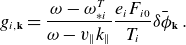
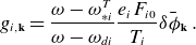
 \begin{equation} \begin{gathered} \frac {\partial g_{a,\mathbf{k}}}{\partial t}+v_{\parallel }\frac {\partial g_{a,\mathbf{k}}}{\partial l}+i\omega _{da}g_{a,\mathbf{k}}-\frac {1}{B^2}\sum _{\mathbf{k^{'}}}\mathbf{B}\cdot (\mathbf{k}\times \mathbf{k^{'}})\bar {\delta \phi _{\mathbf{k}}}g_{a,\mathbf{k}-\mathbf{k}^{'}}\\ =\sum _b[C_{ab}(g_{a,\mathbf{k}},F_{b0})+C_{ab}(F_{a0},g_{b,\mathbf{k}})]+\frac {e_aF_{a0}}{T_a}\left (\frac {\partial }{\partial t}+i\omega _{*a}^T\right )\bar {\delta \phi _{\mathbf{k}}}\; , \end{gathered} \end{equation}
with ${\delta \bar{\phi} _{\mathbf{k}}}=J_0\left (k_{\perp }v_{\perp }/\Omega _a\right )\delta \phi _{\mathbf{k}}$
the gyroaveraged electrostatic potential fluctuations. The equation describes the evolution of the non-adiabatic part of the perturbed distribution function for the particle species
${\delta \bar{\phi} _{\mathbf{k}}}=J_0\left (k_{\perp }v_{\perp }/\Omega _a\right )\delta \phi _{\mathbf{k}}$
the gyroaveraged electrostatic potential fluctuations. The equation describes the evolution of the non-adiabatic part of the perturbed distribution function for the particle species $a$
,
$a$
,
 \begin{equation} f_a(\mathbf{r},E_a,\mu _a,t)=F_{a0}(\psi ,E_a)\left (1-\frac {e_a\delta \phi (\mathbf{r})}{T_a}\right )+g_a(\mathbf{R},E_a,\mu _a,t)\; , \end{equation}
having a Maxwellian equilibrium distribution function $F_{a0}$
with temperature
$F_{a0}$
with temperature $T_a(\psi )$
, density
$T_a(\psi )$
, density $n_a(\psi )$
, mass
$n_a(\psi )$
, mass $m_a$
and charge
$m_a$
and charge $e_a$
. The particle position is
$e_a$
. The particle position is $\mathbf{r}$
and
$\mathbf{r}$
and $\mathbf{R}=\mathbf{r}-\mathbf{b}\times \boldsymbol{v}/{}\Omega _a$
is the gyrocentre position, with
$\mathbf{R}=\mathbf{r}-\mathbf{b}\times \boldsymbol{v}/{}\Omega _a$
is the gyrocentre position, with $\Omega _a=e_aB/m_a$
the gyrofrequency. Flux-tube geometry is assumed and the magnetic field
$\Omega _a=e_aB/m_a$
the gyrofrequency. Flux-tube geometry is assumed and the magnetic field $\mathbf{B}=B(l)\mathbf{b}=\nabla \psi \times \nabla \alpha$
is written in terms of Clebsh coordinates
$\mathbf{B}=B(l)\mathbf{b}=\nabla \psi \times \nabla \alpha$
is written in terms of Clebsh coordinates $(\psi ,\alpha )$
. The instability wavenumber can thus be decomposed as
$(\psi ,\alpha )$
. The instability wavenumber can thus be decomposed as $\mathbf{k}=\mathbf{k}_{\perp }=k_{\psi }\nabla \psi +k_{\alpha }\nabla \alpha$
, with
$\mathbf{k}=\mathbf{k}_{\perp }=k_{\psi }\nabla \psi +k_{\alpha }\nabla \alpha$
, with $\nabla \psi$
and
$\nabla \psi$
and $\nabla \alpha$
functions of the arc length
$\nabla \alpha$
functions of the arc length $l$
along magnetic field lines, while
$l$
along magnetic field lines, while $k_{\psi }$
and
$k_{\psi }$
and $k_{\alpha }$
are independent of it. The optimal-mode theory discussed in the next section will thus be applicable to local instabilities, although the underlying thermodynamic principles hold more generally. The particle velocity can be decomposed as
$k_{\alpha }$
are independent of it. The optimal-mode theory discussed in the next section will thus be applicable to local instabilities, although the underlying thermodynamic principles hold more generally. The particle velocity can be decomposed as $\boldsymbol{v}=v_{\parallel }\mathbf{b}+\boldsymbol{v}_{\perp }$
, and all derivatives in (2.1) are taken at constant unperturbed energy
$\boldsymbol{v}=v_{\parallel }\mathbf{b}+\boldsymbol{v}_{\perp }$
, and all derivatives in (2.1) are taken at constant unperturbed energy $E_a=m_a v^2/2 + e_a\Phi (\psi )$
and magnetic moment
$E_a=m_a v^2/2 + e_a\Phi (\psi )$
and magnetic moment $\mu _a=m_a v_{\perp }^2/(2B)$
.
$\mu _a=m_a v_{\perp }^2/(2B)$
.
In this work, we limit ourselves to the study of electrostatic microinstabilities, where the electrostatic potential fluctuations $\delta \phi$
are given by the quasineutrality condition
$\delta \phi$
are given by the quasineutrality condition
 \begin{equation} \sum _a\lambda _a\delta \phi _{\mathbf{k}}=\sum _a e_a\int g_{a,\mathbf{k}}J_{0a}\text{d}^{3}v\; , \end{equation}
where $\lambda _a=n_a e_a^2/T_a$
and
$\lambda _a=n_a e_a^2/T_a$
and $J_{na}=J_n(k_{\perp } v_{\perp }/\Omega _a)$
. The remaining terms in the gyrokinetic equation (2.1) are the drift frequency
$J_{na}=J_n(k_{\perp } v_{\perp }/\Omega _a)$
. The remaining terms in the gyrokinetic equation (2.1) are the drift frequency $\omega _{da}=\mathbf{k}\cdot \boldsymbol{v}_{da}$
, with
$\omega _{da}=\mathbf{k}\cdot \boldsymbol{v}_{da}$
, with $\boldsymbol{v}_{da}$
the unperturbed drift velocity, and the diamagnetic frequencies
$\boldsymbol{v}_{da}$
the unperturbed drift velocity, and the diamagnetic frequencies
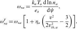 \begin{equation} \begin{gathered} \omega _{*a}=\frac {k_{\alpha }T_a}{e_a}\frac {\mathrm{d}\ln {n_a}}{\mathrm{d}\psi },\\ \omega _{*a}^T=\omega _{*a}\left [1+\eta _a \left (\frac {v^2}{2v_{th,a}^2}-\frac {3}{2}\right )\right ]\!, \end{gathered} \end{equation}
with $\eta _a=(\text{d}\ln {T_a}/\text{d} \psi )/(\text{d}\ln {n_a}/\text{d}\psi )$
and
$\eta _a=(\text{d}\ln {T_a}/\text{d} \psi )/(\text{d}\ln {n_a}/\text{d}\psi )$
and $v_{th,a}=\sqrt {T_a/m_a}$
the species thermal velocity. Finally,
$v_{th,a}=\sqrt {T_a/m_a}$
the species thermal velocity. Finally, $C_{ab}$
is the collision operator between species
$C_{ab}$
is the collision operator between species $a$
and
$a$
and $b$
.
$b$
.
The optimal-mode theory follows from thermodynamic considerations on the gyrokinetic equation. Specifically, an equation for the Helmholtz free energy budget is derived by applying the following operation to (2.1):
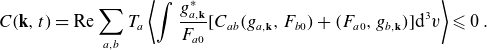
 \begin{equation} \text{Re} \sum _{a,\mathbf{k}}T_a\left \langle \int (\ldots ) \frac {g_{a,\mathbf{k}}^*}{F_{a0}}\text{d}^{3}v\right \rangle. \end{equation}
This operation and its effect on the gyrokinetic equation are explained in detail in Part 1 (Helander & Plunk Reference Helander and Plunk2022), with only the key points summarised here. Notably, this operation causes both the nonlinear term and all terms explicitly dependent on the geometry to vanish. This latter effect is why the resulting upper bounds are applicable to any type of plasma geometry. The remaining terms in the equation can then be reorganised to yield the Helmholtz free energy budget,
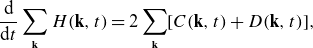 \begin{equation} \frac {\mathrm{d}}{\mathrm{d}t}\sum _{\mathbf{k}}H(\mathbf{k},t)=2\sum _{\mathbf{k}}[C(\mathbf{k},t)+D(\mathbf{k},t)], \end{equation}
with $H$
the Helmholtz free energy of fluctuations,
$H$
the Helmholtz free energy of fluctuations,
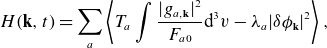 \begin{equation} H(\mathbf{k},t)=\sum _a\left \langle T_a\int \frac {| g_{a,\mathbf{k}}|^2}{F_{a0}}\text{d}^{3}v-\lambda _a|\delta \phi _{\mathbf{k}}|^2\right \rangle, \end{equation} $D$
the drive term,
$D$
the drive term,
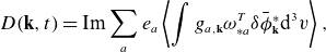 \begin{equation} D(\mathbf{k},t)=\text{Im}\sum _a e_a\left \langle \int g_{a,\mathbf{k}}\omega _{*a}^T\bar {\delta \phi _{\mathbf{k}}^*}\text{d}^{3}v\right \rangle, \end{equation}
and $C$
the collisional term, which is always negative or vanishes by Boltzmann’s
$C$
the collisional term, which is always negative or vanishes by Boltzmann’s $H$
-theorem,
$H$
-theorem,
 \begin{equation} C(\mathbf{k},t)=\text{Re}\sum _{a,b} T_a\left \langle \int \frac {g_{a,\mathbf{k}}^*}{F_{a0}}[C_{ab}(g_{a,\mathbf{k}},F_{b0})+(F_{a0},g_{b,\mathbf{k}})]\text{d}^{3}v\right \rangle \leqslant 0\; . \end{equation}
Equation (2.6) is the starting point for the derivation of upper bounds on linear and nonlinear growth rates (Helander & Plunk Reference Helander and Plunk2021). From Boltzmann’s $H$
-theorem, it indeed follows that the instabilities linear growth rate is bounded from above,
$H$
-theorem, it indeed follows that the instabilities linear growth rate is bounded from above,
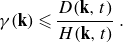 \begin{equation} \gamma (\mathbf{k})\leqslant \frac {D(\mathbf{k},t)}{H(\mathbf{k},t)}\; . \end{equation}
For the ratio $D/H$
to serve as a suitable bound, it must be bounded from above: it must be smaller than some finite number for any set of distribution functions
$D/H$
to serve as a suitable bound, it must be bounded from above: it must be smaller than some finite number for any set of distribution functions $g_{a,\textbf {k}}$
. The primary challenge in proving this result lies in identifying an appropriate lower bound for
$g_{a,\textbf {k}}$
. The primary challenge in proving this result lies in identifying an appropriate lower bound for $H(\mathbf{k},t)$
. In the following paragraphs, we review methods for achieving this goal and obtaining tight bounds in different cases relevant to this work, starting with the simplest case and progressing to more general ones.
$H(\mathbf{k},t)$
. In the following paragraphs, we review methods for achieving this goal and obtaining tight bounds in different cases relevant to this work, starting with the simplest case and progressing to more general ones.
2.1. Adiabatic electrons
The simplest case for deriving the upper bound is that of an electrostatic, hydrogen plasma with adiabatic electrons. As detailed in Part 1, in this limit, $D$
and
$D$
and $H$
are quadratic functionals of
$H$
are quadratic functionals of $g=g_{i,\mathbf{k}}$
, the perturbed ion distribution function. The optimal upper bound is obtained by maximising the ratio
$g=g_{i,\mathbf{k}}$
, the perturbed ion distribution function. The optimal upper bound is obtained by maximising the ratio $D[g]/H[g]$
over all possible distribution functions
$D[g]/H[g]$
over all possible distribution functions $g$
. This maximisation is achieved by minimising
$g$
. This maximisation is achieved by minimising $H[g]$
, which leads to the identification of the aforementioned optimal modes. These modes take the form
$H[g]$
, which leads to the identification of the aforementioned optimal modes. These modes take the form
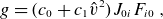 \begin{equation} g=(c_0+c_1\hat {v}^2)J_{0i}F_{i0}\; , \end{equation}
where $c_0$
and
$c_0$
and $c_1$
are the Lagrange multipliers used to minimise
$c_1$
are the Lagrange multipliers used to minimise $H[g]$
, and
$H[g]$
, and $\hat {v}=m_iv^2/2T_i$
. As shown in Part 1, the problem of constructing optimal modes is thus reduced to the question of determining these two constants. These modes realise optimal, instantaneous growth of free energy and differ from normal modes, which satisfy (2.1). In particular, we underline they contain no information on the geometry.
$\hat {v}=m_iv^2/2T_i$
. As shown in Part 1, the problem of constructing optimal modes is thus reduced to the question of determining these two constants. These modes realise optimal, instantaneous growth of free energy and differ from normal modes, which satisfy (2.1). In particular, we underline they contain no information on the geometry.
To obtain the best upper bound
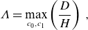 \begin{equation} \unicode{x1D6EC} =\max _{c_0,c_1}\left (\frac {D}{H}\right )\; , \end{equation}
we take the variations of $H$
and
$H$
and $D$
, so that
$D$
, so that
 \begin{equation} \delta D=\unicode{x1D6EC} \delta H\; . \end{equation}
This equation describes a two-dimensional eigenproblem having as non-trivial solutions
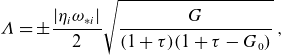 \begin{equation} \unicode{x1D6EC} =\pm \frac {|\eta _i\omega _{*i}|}{2}\sqrt {\frac {G}{(1+\tau )(1+\tau -G_0)}}\; , \end{equation}
with $\tau =T_i/T_e$
, and
$\tau =T_i/T_e$
, and
 \begin{equation} \begin{gathered} G_0(b_i)=\unicode{x1D6E4} _0(b_i),\\ G_1(b_i)=\left ( \frac {3}{2}-b_i\right )\unicode{x1D6E4} _0(b_i)+b_i\unicode{x1D6E4} _1(b_i),\\ G_2(b_i)=\left ( \frac {15}{4}-5b_i+2b_i^2\right )\unicode{x1D6E4} _0(b_i)+(4-2b_i)b_i\unicode{x1D6E4} _1(b_i),\\ G(b_i)=G_0(b_i)G_2(b_i)-G_1^2(b_i).\\ \end{gathered} \end{equation}
Here, $\unicode{x1D6E4} _n(b_i)=I_n(b_i)\text{e}^{-b_i}$
, with
$\unicode{x1D6E4} _n(b_i)=I_n(b_i)\text{e}^{-b_i}$
, with $I_n$
denoting modified Bessel functions and
$I_n$
denoting modified Bessel functions and $b_i\equiv k_{\perp }^2\rho _i^2=k_{\perp }^2T_i/(m_i\Omega _i^2)$
.
$b_i\equiv k_{\perp }^2\rho _i^2=k_{\perp }^2T_i/(m_i\Omega _i^2)$
.
An upper bound on the linear growth rate of instabilities is obtained by choosing the positive eigenvalue of (2.14). The negative eigenvalue indicates a decrease in free energy and is thus linked to damped modes. Notably, this upper bound depends only on a few parameters: the density and temperature gradients, encapsulated by $\eta _i\omega _{*i}$
, the ratio of ion-to-electron temperatures
$\eta _i\omega _{*i}$
, the ratio of ion-to-electron temperatures $\tau$
, and the perpendicular wavenumber, through
$\tau$
, and the perpendicular wavenumber, through $b_i$
. This last parameter hides an implicit dependency on geometry, as the value of
$b_i$
. This last parameter hides an implicit dependency on geometry, as the value of $k_{\perp }(l)$
varies along the magnetic field line. However, the optimal modes exhibit a
$k_{\perp }(l)$
varies along the magnetic field line. However, the optimal modes exhibit a $\delta (l-l_0)$
spatial dependency and thus only depend on the magnetic field at one single location along the flux tube under consideration. Specifically,
$\delta (l-l_0)$
spatial dependency and thus only depend on the magnetic field at one single location along the flux tube under consideration. Specifically, $l_0$
is selected by the criterion (Helander & Plunk Reference Helander and Plunk2022)
$l_0$
is selected by the criterion (Helander & Plunk Reference Helander and Plunk2022)
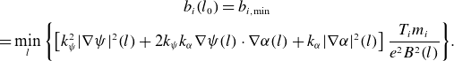 \begin{equation} \begin{gathered} b_i(l_0)=b_{i,\min }\\ =\min _{l}\left \{ \left [k_{\psi }^2|\nabla \psi |^2(l)+2k_{\psi }k_{\alpha }\nabla \psi (l)\cdot \nabla \alpha (l) + k_{\alpha }|\nabla \alpha |^2(l)\right ]\frac {T_i m_i}{e^2B^2(l)}\right \}\!. \end{gathered} \end{equation}
In fact, much of the explicit geometry dependency was already eliminated by applying the operation defined in (2.5). As a result, the upper bound becomes spatially local, both across and along magnetic field lines. This localisation implies that the upper bound serves as a constraint on the linear growth rate of local gyrokinetic instabilities in any flux-tube magnetic geometry.
Under the assumptions of an electrostatic, hydrogen plasma with adiabatic electrons, this bound is applicable to ion temperature gradient (ITG) and trapped-ion instabilities. We highlight two significant limits of the upper bound, which correspond to the opposite extremes of the $b_i$
domain, namely the small and large ones:
$b_i$
domain, namely the small and large ones:
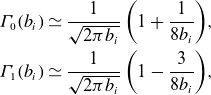
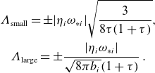 \begin{equation} \begin{gathered} \unicode{x1D6EC} _{\text{small}}=\pm |\eta _i\omega _{*i}|\sqrt {\frac {3}{8\tau (1+\tau )}},\\ \unicode{x1D6EC} _{\text{large}}=\pm \frac {|\eta _i\omega _{*i}|}{\sqrt {8\pi b_i}(1+\tau )}\; . \end{gathered} \end{equation}
To extend the upper bound to any plasma $\beta$
and any number of kinetic particle species, a more general approach is required. This broader framework allows the upper bound to encompass the description of all gyrokinetic instabilities in a flux tube.
$\beta$
and any number of kinetic particle species, a more general approach is required. This broader framework allows the upper bound to encompass the description of all gyrokinetic instabilities in a flux tube.
2.2. Kinetic electrons
The computation of the upper bound follows a similar mathematical approach also when kinetic electrons are included. The objective remains to maximise the ratio $\unicode{x1D6EC} =D/H$
and the way it is achieved is through a variational problem, as in (2.13). The eigenvalue problem to be solved is
$\unicode{x1D6EC} =D/H$
and the way it is achieved is through a variational problem, as in (2.13). The eigenvalue problem to be solved is
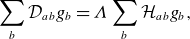 \begin{equation} \sum _b\mathcal{D}_{ab}g_b=\unicode{x1D6EC} \sum _b\mathcal{H}_{ab}g_b, \end{equation}
with $a$
and
$a$
and $b$
denoting particle species indices, and
$b$
denoting particle species indices, and $\mathcal{D}$
and
$\mathcal{D}$
and $\mathcal{H}$
purely imaginary and purely real Hermitian linear operators on the space of distribution functions. Their form is given in more detail in Part 2.
$\mathcal{H}$
purely imaginary and purely real Hermitian linear operators on the space of distribution functions. Their form is given in more detail in Part 2.
In general, $\mathcal{D}$
and
$\mathcal{D}$
and $\mathcal{H}$
are functions of both
$\mathcal{H}$
are functions of both $g_{i,\mathbf{k}}$
and
$g_{i,\mathbf{k}}$
and $g_{e,\mathbf{k}}$
, but they depend on a small set of velocity moments of these distribution functions. By considering linear combinations of these velocity moments, we can reduce the problem to a closed linear system, thereby decreasing its dimensionality. In the full electromagnetic case, (2.18) represents a
$g_{e,\mathbf{k}}$
, but they depend on a small set of velocity moments of these distribution functions. By considering linear combinations of these velocity moments, we can reduce the problem to a closed linear system, thereby decreasing its dimensionality. In the full electromagnetic case, (2.18) represents a $6N_s$
-dimensional eigenproblem, where
$6N_s$
-dimensional eigenproblem, where $N_s$
is the number of particle species. However, when using linear combinations of the velocity moments, the dimensionality is reduced to just 6 for any number of species. This reduction is useful as it ensures the upper bounds are easily calculated in any multi-species plasma.
$N_s$
is the number of particle species. However, when using linear combinations of the velocity moments, the dimensionality is reduced to just 6 for any number of species. This reduction is useful as it ensures the upper bounds are easily calculated in any multi-species plasma.
For electrostatic instabilities, the final problem to solve is a two-dimensional algebraic system. When the spatial dependency is assumed to be $\delta (l-l_0)$
, the solutions to (2.18) form a complete and orthogonal basis for the space of distribution functions. The upper bound is again determined by the positive eigenvalue of the algebraic problem described by (2.18). However, the form of this eigenvalue is more complex than the one in (2.14). Therefore, we will present only its asymptotic limits, which were derived in Part 2, for the scenarios relevant to our present purposes.
$\delta (l-l_0)$
, the solutions to (2.18) form a complete and orthogonal basis for the space of distribution functions. The upper bound is again determined by the positive eigenvalue of the algebraic problem described by (2.18). However, the form of this eigenvalue is more complex than the one in (2.14). Therefore, we will present only its asymptotic limits, which were derived in Part 2, for the scenarios relevant to our present purposes.
We again consider a hydrogen plasma and derive the asymptotic limits for ITG modes in the presence of an ion temperature gradient only. Our primary interest lies in comparing normal modes and optimal modes characterised by small to intermediate wavenumbers. To understand the relevant order of magnitude, we use the expansion parameter
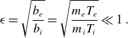 \begin{equation} \epsilon =\sqrt {\frac {b_e}{b_i}}=\sqrt {\frac {m_eT_e}{m_iT_i}}\ll 1\; . \end{equation}
In the small-wavenumber limit, where $b_i\sim \epsilon$
and
$b_i\sim \epsilon$
and $b_e\sim \epsilon ^3$
, the upper bound for an electrostatic, hydrogen plasma, with kinetic electrons and an ion temperature gradient, can be approximated by
$b_e\sim \epsilon ^3$
, the upper bound for an electrostatic, hydrogen plasma, with kinetic electrons and an ion temperature gradient, can be approximated by
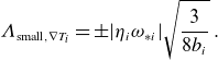 \begin{equation} \unicode{x1D6EC} _{\text{small}, \nabla T_i}=\pm |\eta _i\omega _{*i}|\sqrt {\frac {3}{8b_i}}\; . \end{equation}
For intermediate wavenumbers, where $b_i\sim \epsilon ^{-1}$
and
$b_i\sim \epsilon ^{-1}$
and $b_e\sim \epsilon$
, the upper bound instead becomes
$b_e\sim \epsilon$
, the upper bound instead becomes
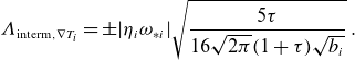 \begin{equation} \unicode{x1D6EC} _{\text{interm}, \nabla T_i}=\pm |\eta _i\omega _{*i}|\sqrt {\frac {5\tau }{16\sqrt {2\pi }(1+\tau )\sqrt {b_i}}}\; . \end{equation}
To estimate the range of validity for these asymptotic limits, we note that in an equithermal ( $\tau =1$
) hydrogen plasma,
$\tau =1$
) hydrogen plasma, $\epsilon \approx 0.02$
. In the same range of validity, the asymptotic trends of the upper bound for an electrostatic, hydrogen plasma, with kinetic electrons and a density gradient only, are
$\epsilon \approx 0.02$
. In the same range of validity, the asymptotic trends of the upper bound for an electrostatic, hydrogen plasma, with kinetic electrons and a density gradient only, are
 \begin{equation} \begin{gathered} \unicode{x1D6EC} _{\text{small}, \nabla n}=\pm |\omega _{*i}|\sqrt {\frac {\tau }{(1+\tau )b_i}}\; ,\\ \unicode{x1D6EC} _{\text{interm}, \nabla n}=\pm |\omega _{*i}|\sqrt {\frac {\tau }{\sqrt {2\pi }(1+\tau )\sqrt {b_i}}}\; . \end{gathered} \end{equation}
Using these asymptotic limits, we will provide an upper bound for trapped-particle instabilities driven by density gradients. In all the reported scenarios, the upper bound remains dependent on a limited set of parameters. We will discuss the trends of these upper bounds and their asymptotic limits in § 4.
3. Normal-mode solutions in simplified geometries
In contrast to optimal modes, normal modes are solutions to the linearised gyrokinetic equation (2.1). To solve the equation, a typical approach involves solving an initial value problem. In this work, we will mainly compute normal modes by solving the linear gyrokinetic equation with the $\delta f$
-gyrokinetic code stella (Barnes et al. Reference Barnes, Parra and Landreman2019). The initial distribution function
$\delta f$
-gyrokinetic code stella (Barnes et al. Reference Barnes, Parra and Landreman2019). The initial distribution function $g_a(\mathbf{R},E_a,\mu _a,t=0)$
is set to be a Maxwellian, with a Gaussian structure along the magnetic field line. The equation is evolved till the solution matches an exponential behaviour of the type
$g_a(\mathbf{R},E_a,\mu _a,t=0)$
is set to be a Maxwellian, with a Gaussian structure along the magnetic field line. The equation is evolved till the solution matches an exponential behaviour of the type $\exp (-i\omega t)$
. We consider the simulation to be converged when the average value of
$\exp (-i\omega t)$
. We consider the simulation to be converged when the average value of $\omega$
over the last 10 % of the simulation exhibits a relative error of only a few percent.
$\omega$
over the last 10 % of the simulation exhibits a relative error of only a few percent.
Gyrokinetic codes allow for the solution of the gyrokinetic equation in magnetic fields of any complexity. For simpler magnetic equilibria, analytically treatable dispersion relations can be derived. In § 4, we will compare the upper bounds derived in § 2 with results from two such cases: a plasma slab and a purely toroidal plasma. Specifically, we will examine an electrostatic, collisionless hydrogen plasma with adiabatic electrons, focusing on the derivation of the ITG mode dispersion relations.
3.1. Slab ITG dispersion relation
We first consider the case of a plasma slab (Kadomtsev & Pogutse Reference Kadomtsev and Pogutse1970; Cowley et al. Reference Cowley, Kulsrud and Sudan1991), which applies when the curvature drift is negligible $\omega _{di}=0$
and the magnetic field strength is constant. The mode is thus not confined to any location along magnetic field lines and we can assume the solution to the gyrokinetic equation to be a plane wave
$\omega _{di}=0$
and the magnetic field strength is constant. The mode is thus not confined to any location along magnetic field lines and we can assume the solution to the gyrokinetic equation to be a plane wave $g_{i,\mathbf{k}}\propto \exp (ik_{\parallel }l-i\omega t)$
. The gyrokinetic equation (2.1) thus yields
$g_{i,\mathbf{k}}\propto \exp (ik_{\parallel }l-i\omega t)$
. The gyrokinetic equation (2.1) thus yields
 \begin{equation} g_{i,\mathbf{k}}=\frac {\omega -\omega _{*i}^T}{\omega - v_{\parallel }k_{\parallel }}\frac {e_iF_{i0}}{T_i}\bar {\delta \phi _{\mathbf{k}}}\; . \end{equation}
To get the dispersion relation, we substitute this result into the quasineutrality condition (2.3), and after computing the velocity integrals and writing everything in terms of the plasma dispersion function $Z(\zeta )$
(Fried & Conte Reference Fried and Conte1961), we obtain
$Z(\zeta )$
(Fried & Conte Reference Fried and Conte1961), we obtain
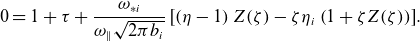
 \begin{equation} \begin{gathered} 0=1+\tau +\unicode{x1D6E4} _0\left \{ \zeta Z(\zeta )+\frac {\omega _{*i}}{\omega _{\parallel }}\left [\left (\frac {3\eta _i}{2}-1\right )Z(\zeta )-\zeta \eta _i\left (1+\zeta Z(\zeta )\right )\right ]\right \}\\ -\frac {\omega _{*i}}{\omega _{\parallel }}\eta _i\left [(1-b_i)\unicode{x1D6E4} _0+b_i\unicode{x1D6E4} _1\right ]Z(\zeta )\; . \end{gathered} \end{equation}
Here, $\tau =T_i/T_e$
,
$\tau =T_i/T_e$
, $\unicode{x1D6E4} _n=\unicode{x1D6E4} _n(b_i)=I_n(b_i)\text{e}^{-b_i}$
, with
$\unicode{x1D6E4} _n=\unicode{x1D6E4} _n(b_i)=I_n(b_i)\text{e}^{-b_i}$
, with $I_n$
modified Bessel functions and
$I_n$
modified Bessel functions and $b_i\equiv k_{\perp }^2\rho _i^2=k_{\perp }^2T_i/(m_i\Omega _i^2)$
. We have also defined
$b_i\equiv k_{\perp }^2\rho _i^2=k_{\perp }^2T_i/(m_i\Omega _i^2)$
. We have also defined $\omega _{\parallel }=k_{\parallel }v_{th,i}$
and
$\omega _{\parallel }=k_{\parallel }v_{th,i}$
and $\zeta =\omega /\omega _{\parallel }$
.
$\zeta =\omega /\omega _{\parallel }$
.
It is instructive to consider the limit of short wavelength, $b_i \rightarrow \infty$
, where
$b_i \rightarrow \infty$
, where
 \begin{equation} \begin{gathered} \unicode{x1D6E4} _0(b_i) \simeq \frac {1}{\sqrt {2 \pi b_i}} \left ( 1 + \frac {1}{8 b_i} \right )\!,\\ \unicode{x1D6E4} _1(b_i) \simeq \frac {1}{\sqrt {2 \pi b_i}} \left ( 1 - \frac {3}{8 b_i} \right )\!, \end{gathered} \end{equation}
and the dispersion relation (3.2) thus reduces to
 \begin{equation} 0=1+\tau +\frac {\omega _{*i}}{\omega _{\parallel } \sqrt {2 \pi b_i}} \left [\left (\eta -1\right )Z(\zeta )-\zeta \eta _i\left (1+\zeta Z(\zeta )\right ) \right ]\!. \end{equation}
In this equation, $\omega _{*i} / \sqrt {b_i}$
is independent of
$\omega _{*i} / \sqrt {b_i}$
is independent of $k_\perp$
, which thus drops out of the equation. It follows that the growth rate
$k_\perp$
, which thus drops out of the equation. It follows that the growth rate $\gamma = \omega _\parallel \Im[\zeta]$
is also independent of
$\gamma = \omega _\parallel \Im[\zeta]$
is also independent of $k_\perp$
. In other words, the growth rate approaches a finite, non-zero constant in the short-wavelength limit,
$k_\perp$
. In other words, the growth rate approaches a finite, non-zero constant in the short-wavelength limit, $b_i \rightarrow \infty$
, despite the decay of the Bessel functions. This behaviour is very different from that of gyrokinetic instabilities in tokamak or stellarator geometry, which tend to be stable at sufficiently short wavelengths.
$b_i \rightarrow \infty$
, despite the decay of the Bessel functions. This behaviour is very different from that of gyrokinetic instabilities in tokamak or stellarator geometry, which tend to be stable at sufficiently short wavelengths.
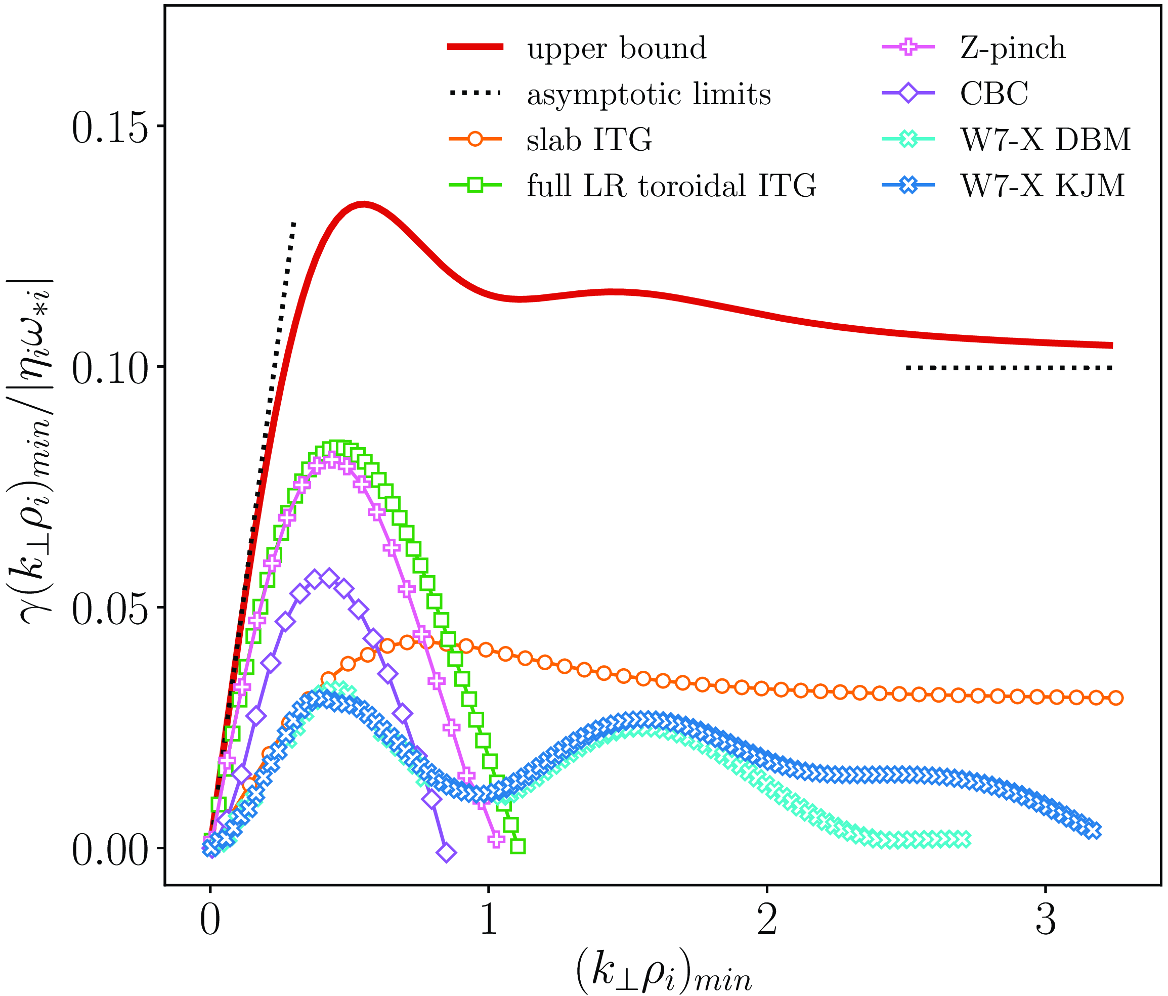
Figure 1. Upper bound for an electrostatic and collisionless hydrogen plasma with $\tau =1$
and adiabatic electrons (2.14) compared with results from gyrokinetic simulations and analytically derived toroidal and slab ITG dispersion relations.
$\tau =1$
and adiabatic electrons (2.14) compared with results from gyrokinetic simulations and analytically derived toroidal and slab ITG dispersion relations.
For the comparison with upper bounds, we examine the growth rate derived from the dispersion relation (3.2) as a function of the perpendicular wavenumber $k_{\perp }\rho _i$
. The latter appears in (3.2) in the diamagnetic frequency
$k_{\perp }\rho _i$
. The latter appears in (3.2) in the diamagnetic frequency $\omega _{*i}$
and in
$\omega _{*i}$
and in $b_i$
. The parallel wavenumber
$b_i$
. The parallel wavenumber $k_{\parallel }$
is a free parameter. To find the largest growth rate for each
$k_{\parallel }$
is a free parameter. To find the largest growth rate for each $k_{\perp }\rho _i$
, we fix
$k_{\perp }\rho _i$
, we fix $k_{\perp }\rho _i$
and we vary
$k_{\perp }\rho _i$
and we vary $k_{\parallel }$
to find the root of (3.2) that maximises the growth rate for a given set of
$k_{\parallel }$
to find the root of (3.2) that maximises the growth rate for a given set of $\tau$
,
$\tau$
, $\omega _{*i}$
and
$\omega _{*i}$
and $\eta _i$
. The result is shown in § 4, in the comparison between the upper bound and normal-mode growth rates for a plasma with adiabatic electrons (figure 1).
$\eta _i$
. The result is shown in § 4, in the comparison between the upper bound and normal-mode growth rates for a plasma with adiabatic electrons (figure 1).
3.2. Toroidal ITG dispersion relation
To derive the toroidal ITG dispersion relation, a similar approach is employed. We assume an exponential temporal behaviour for the non-adiabatic part of the perturbed distribution function, $g_{i,\mathbf{k}}\propto \exp (-i\omega t)$
. We then adopt a local approximation by neglecting streaming along magnetic field lines, which is equivalent to assuming that
$g_{i,\mathbf{k}}\propto \exp (-i\omega t)$
. We then adopt a local approximation by neglecting streaming along magnetic field lines, which is equivalent to assuming that $\omega _{\parallel }\ll \omega$
. It follows that (2.1) can be rewritten as
$\omega _{\parallel }\ll \omega$
. It follows that (2.1) can be rewritten as
 \begin{equation} g_{i,\mathbf{k}}=\frac {\omega -\omega _{*i}^T}{\omega - \omega _{di}}\frac {e_iF_{i0}}{T_i}\bar {\delta \phi _{\mathbf{k}}}\; . \end{equation}
Keeping arbitrary Larmor radius (LR), the resulting dispersion relation (Zocco et al. Reference Zocco, Xanthopoulos, Doerk, Connor and Helander2018) becomes
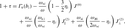 \begin{equation} \begin{split} 1+\tau =\,&\unicode{x1D6E4} _0(b_i)-\frac {\omega _{*i}}{\omega }\left (1-\frac {3}{2}\eta _i\right )J^{(0)}\\ &+\frac {\omega _{*i}}{\omega }\left (\frac {\omega _{\kappa i}}{\omega _{*i}}-\eta _i\right )J_{\parallel }^{(2)}+\frac {\omega _{*i}}{\omega }\left (\frac {\omega _{Bi}}{2\omega _{*i}}-\eta _i\right )J_{\perp }^{(2)}, \end{split} \end{equation}
with $\omega _{\kappa i}$
and
$\omega _{\kappa i}$
and $\omega _{Bi}$
the curvature and
$\omega _{Bi}$
the curvature and $\nabla B$
components of the drift frequency, so that
$\nabla B$
components of the drift frequency, so that
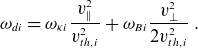 \begin{equation} \omega _{di}=\omega _{\kappa i}\frac {v_{\parallel }^2}{v_{th,i}^2}+\omega _{Bi}\frac {v_{\perp }^2}{2v_{th,i}^2}\; . \end{equation}
For a purely toroidal electrostatic plasma, $\omega _{Bi}=\omega _{\kappa i}=k_y\rho _i v_{th,i}/R$
, with
$\omega _{Bi}=\omega _{\kappa i}=k_y\rho _i v_{th,i}/R$
, with $R$
the average curvature length scale.
$R$
the average curvature length scale. $J^{(0)}$
,
$J^{(0)}$
, $J^{(2)}_{\parallel }$
and
$J^{(2)}_{\parallel }$
and $J^{(2)}_{\perp }$
are trascendental functions of
$J^{(2)}_{\perp }$
are trascendental functions of $\omega _{\kappa i}$
,
$\omega _{\kappa i}$
, $\omega _{Bi}$
and
$\omega _{Bi}$
and $b_i$
and can be found in Appendix B of Zocco et al. Reference Zocco, Xanthopoulos, Doerk, Connor and Helander(2018). Notice that we have corrected a typo
$b_i$
and can be found in Appendix B of Zocco et al. Reference Zocco, Xanthopoulos, Doerk, Connor and Helander(2018). Notice that we have corrected a typo $(J_{\perp }^{(2)}\leftrightarrow J_{\parallel }^{(2)})$
in (B13) of Zocco et al. Reference Zocco, Xanthopoulos, Doerk, Connor and Helander(2018). Taking this correction into account, we calculate the toroidal ITG critical gradient yielded by (3.6) in Appendix A.
$(J_{\perp }^{(2)}\leftrightarrow J_{\parallel }^{(2)})$
in (B13) of Zocco et al. Reference Zocco, Xanthopoulos, Doerk, Connor and Helander(2018). Taking this correction into account, we calculate the toroidal ITG critical gradient yielded by (3.6) in Appendix A.
This dispersion relation reduces to the one derived by Biglari et al. Reference Biglari, Diamond and Rosenbluth(1989) if the drift-kinetic limit ( $b_i\to 0$
) is taken (Zocco et al. Reference Zocco, Xanthopoulos, Doerk, Connor and Helander2018),
$b_i\to 0$
) is taken (Zocco et al. Reference Zocco, Xanthopoulos, Doerk, Connor and Helander2018),
 \begin{equation} 1+\tau = \left (1-\frac {\omega _{*i}}{\omega }\right )\Omega Z^2(\sqrt {\Omega })+\eta _i\frac {\omega _{*i}}{\omega }\left [\left (1-2\Omega \right )\Omega Z^2(\sqrt {\Omega })-2\Omega ^{3/2}Z(\sqrt {\Omega })\right ]\!, \end{equation}
with $\Omega =\omega /\omega _{\kappa i}$
.
$\Omega =\omega /\omega _{\kappa i}$
.
The roots of both dispersion relations need ultimately to be calculated numerically. In Appendix A, we show that they coincide for $b_i\to 0$
and discuss how they compare with results from gyrokinetic simulations.
$b_i\to 0$
and discuss how they compare with results from gyrokinetic simulations.
If we order the frequencies as $\omega _{*i}/\tau \gg \omega \gg \omega _{\kappa i}$
, we can expand the denominator of (3.5). In this way, we are considering the non-resonant limit for which we obtain the strongly driven toroidal-branch dispersion relation
$\omega _{*i}/\tau \gg \omega \gg \omega _{\kappa i}$
, we can expand the denominator of (3.5). In this way, we are considering the non-resonant limit for which we obtain the strongly driven toroidal-branch dispersion relation
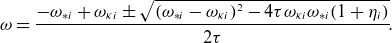 \begin{equation} \omega = \frac {-\omega _{*i}+\omega _{\kappa i}\pm \sqrt {(\omega _{*i}-\omega _{\kappa i})^2-4\tau \omega _{\kappa i}\omega _{*i}(1+\eta _i)}}{2\tau }\!. \end{equation}
This particular ordering allows terms of order $\omega _{\kappa i}/\tau$
to be retained. While they are non-negligible for
$\omega _{\kappa i}/\tau$
to be retained. While they are non-negligible for $\tau \to 0$
, they can be neglected for large
$\tau \to 0$
, they can be neglected for large $\tau$
and the dispersion relation becomes the non-resonant toroidal branch dispersion relation of Biglari et al. Reference Biglari, Diamond and Rosenbluth(1989).
$\tau$
and the dispersion relation becomes the non-resonant toroidal branch dispersion relation of Biglari et al. Reference Biglari, Diamond and Rosenbluth(1989).
We now proceed with the comparison of the results obtained through optimal- and normal-mode theories.
4. Comparing upper bounds with normal-mode growth rates
The main computational task of this paper is to compare the upper bounds with growth rates of normal modes in specific cases. We focus on the electrostatic limit of a collisionless hydrogen plasma with $\tau =1$
. Initially, we consider adiabatic electrons and then we include the effects of kinetic electrons. These scenarios are chosen because they represent the instabilities most harmful to magnetic fusion confinement devices, specifically ion temperature gradient (ITG) modes and trapped electron modes (TEMs).
$\tau =1$
. Initially, we consider adiabatic electrons and then we include the effects of kinetic electrons. These scenarios are chosen because they represent the instabilities most harmful to magnetic fusion confinement devices, specifically ion temperature gradient (ITG) modes and trapped electron modes (TEMs).
For the comparison, we employ electrostatic, collisionless, flux-tube linear simulations using the gyrokinetic code stella. To encompass a wide range of scenarios, we perform simulations across various magnetic fusion devices and plasma gradients. The selected magnetic equilibria include the tokamak Cyclone Base Case (CBC) (Dimits et al. Reference Dimits2000), different magnetic configurations of the stellarator Wendelstein 7-X (W7-X) and the Z-pinch geometry implemented in stella , which is thoroughly discussed and validated in Appendix A.
In
stella
, the Fourier-decomposed linear gyrokinetic equation is normalised by $(a^2/\rho _{\text{ref}} v_{T,\text{ref}})\exp (-v^2/v_{T, a})/F_{a0}$
, where
$(a^2/\rho _{\text{ref}} v_{T,\text{ref}})\exp (-v^2/v_{T, a})/F_{a0}$
, where $a$
represents the effective minor radius and
$a$
represents the effective minor radius and $\rho _{\text{ref}}=v_{T,\text{ref}}/\Omega _{\text{ref}}$
is the Larmor radius of the reference species, characterised by thermal velocity
$\rho _{\text{ref}}=v_{T,\text{ref}}/\Omega _{\text{ref}}$
is the Larmor radius of the reference species, characterised by thermal velocity $v_{T,\text{ref}}=\sqrt {2T_{\text{ref}}/m_{\text{ref}}}$
, mass
$v_{T,\text{ref}}=\sqrt {2T_{\text{ref}}/m_{\text{ref}}}$
, mass $m_{\text{ref}}$
and temperature
$m_{\text{ref}}$
and temperature $T_{\text{ref}}$
.Footnote
1
The phase-space coordinates used in stella are
$T_{\text{ref}}$
.Footnote
1
The phase-space coordinates used in stella are $(x,y,z,v_{\parallel },\mu )$
. The plane perpendicular to the magnetic field lines is parametrised by the radial and binormal coordinates
$(x,y,z,v_{\parallel },\mu )$
. The plane perpendicular to the magnetic field lines is parametrised by the radial and binormal coordinates $(x,y)$
, which measure the distance from the magnetic field line at the centre of the flux tube:
$(x,y)$
, which measure the distance from the magnetic field line at the centre of the flux tube: $x=\text{d} x/\text{d} \psi |_{\psi _0}(\psi -\psi _0)$
and
$x=\text{d} x/\text{d} \psi |_{\psi _0}(\psi -\psi _0)$
and $y=\text{d} y/\text{d} \alpha |_{\alpha _0}(\alpha -\alpha _0)$
. The definitions of
$y=\text{d} y/\text{d} \alpha |_{\alpha _0}(\alpha -\alpha _0)$
. The definitions of $\text{d} x/\text{d} \psi |_{\psi _0}$
and
$\text{d} x/\text{d} \psi |_{\psi _0}$
and $\text{d} y/\text{d} \alpha |_{\alpha _0}$
depend on the choice of magnetic geometry (see e.g. Barnes et al. Reference Barnes, Parra and Landreman(2019) and Appendix A).
$\text{d} y/\text{d} \alpha |_{\alpha _0}$
depend on the choice of magnetic geometry (see e.g. Barnes et al. Reference Barnes, Parra and Landreman(2019) and Appendix A).
The inverse gradient scale length for a given quantity $X$
is defined as
$X$
is defined as
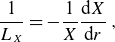 \begin{equation} \frac {1}{L_{X}}=-\frac {1}{X}\frac {\mathrm{d} X}{\mathrm{d} r}\;, \end{equation}
with $r$
the effective minor radius of the device. The gradient scale length is then normalised by the scale length of the magnetic field variation, here denoted with
$r$
the effective minor radius of the device. The gradient scale length is then normalised by the scale length of the magnetic field variation, here denoted with $a$
. In
stella
, this is chosen to be the effective minor radius at the last closed flux-surface, both for tokamak CBC and W7-X magnetic geometries, while in the case of a Z-pinch, it coincides with the cylinder radius (table 1 and Appendix A).
$a$
. In
stella
, this is chosen to be the effective minor radius at the last closed flux-surface, both for tokamak CBC and W7-X magnetic geometries, while in the case of a Z-pinch, it coincides with the cylinder radius (table 1 and Appendix A).
Table 1. Geometric parameters for the different devices simulated: a tokamak Cyclone Base Case (CBC), two different W7-X magnetic configurations: high-mirror (KJM) and low-iota (DBM) and lastly, the Z-pinch geometry.

The simulations are conducted with the resolution $N_z\times N_{v_{\parallel }}\times N_{\mu }=96\times 36\times 24$
. The minimum simulated binormal wavenumber is
$N_z\times N_{v_{\parallel }}\times N_{\mu }=96\times 36\times 24$
. The minimum simulated binormal wavenumber is $\Delta k_y\rho _i\approx 0.07$
, with the total number of wavenumbers varying depending on the equilibrium. The radial wavenumber is set to zero,
$\Delta k_y\rho _i\approx 0.07$
, with the total number of wavenumbers varying depending on the equilibrium. The radial wavenumber is set to zero, $k_x\rho _i=0$
. Key geometric parameters, such as the aspect ratio
$k_x\rho _i=0$
. Key geometric parameters, such as the aspect ratio $R/a$
, the radial location of the simulated flux-surface
$R/a$
, the radial location of the simulated flux-surface $r_0/a$
, the safety factor
$r_0/a$
, the safety factor $q$
and the global shear
$q$
and the global shear $\hat {s}$
, depend on the magnetic equilibrium and are listed in table 1. The selected gradients are detailed in the following subsections, where we present the validation results.
$\hat {s}$
, depend on the magnetic equilibrium and are listed in table 1. The selected gradients are detailed in the following subsections, where we present the validation results.
4.1. Pure ITG case
The first comparison is carried out for a plasma with adiabatic electrons and only an ion temperature gradient, as described by (2.14). We compare it with a CBC and two W7-X simulations having $a/L_{Ti}=3$
. The two W7-X configurations include a high-mirror (KJM) and a low-iota (DBM) configuration, with the differences between them detailed in table 1.
$a/L_{Ti}=3$
. The two W7-X configurations include a high-mirror (KJM) and a low-iota (DBM) configuration, with the differences between them detailed in table 1.
Additionally, we solve the dispersion relation for the slab ITG (3.2) with $a/L_{Ti}=3$
and the toroidal ITG with full LR effects (3.6) for
$a/L_{Ti}=3$
and the toroidal ITG with full LR effects (3.6) for $a/L_{Ti}=8.3$
. The latter is compared with a Z-pinch simulation using the same gradient. All the results are presented in figure. 1, where we plot the upper bound and the normal modes growth rates, normalised to
$a/L_{Ti}=8.3$
. The latter is compared with a Z-pinch simulation using the same gradient. All the results are presented in figure. 1, where we plot the upper bound and the normal modes growth rates, normalised to $|\eta _i\omega _{*i}|/(k_{\perp }\rho _i)_{\text{min}}$
, against
$|\eta _i\omega _{*i}|/(k_{\perp }\rho _i)_{\text{min}}$
, against $(k_{\perp }\rho _i)_{\text{min}}$
. The perpendicular wavenumber is taken at the location along the magnetic field line of
$(k_{\perp }\rho _i)_{\text{min}}$
. The perpendicular wavenumber is taken at the location along the magnetic field line of $(k_{\perp }\rho _i)_{\text{min}}=\min _l(k_{\perp }\rho _i)$
as shown in (2.1). The real frequencies associated with the calculated growth rates are provided in figure 11 in Appendix B.
$(k_{\perp }\rho _i)_{\text{min}}=\min _l(k_{\perp }\rho _i)$
as shown in (2.1). The real frequencies associated with the calculated growth rates are provided in figure 11 in Appendix B.
We observe that the upper bound exceeds the growth rates of all the normal modes considered, as it must, and qualitatively follows the trend set by the largest such growth rate. Specifically, for small perpendicular wavenumbers, the upper bound is proportional to $k_\perp \rho _i$
. This is evident from the limit given in (2.1), which, when normalised and for
$k_\perp \rho _i$
. This is evident from the limit given in (2.1), which, when normalised and for $\tau =1$
, reads
$\tau =1$
, reads $\unicode{x1D6EC} (k_{\perp }\rho _i)_{\text{min}}/|\eta _i\omega _{*i}|=\sqrt {3/16}(k_{\perp }\rho _i)_{\text{min}}$
. The upper bound effectively captures the behaviour of the strongly driven toroidal ITG mode, whose dispersion relation is proportional to
$\unicode{x1D6EC} (k_{\perp }\rho _i)_{\text{min}}/|\eta _i\omega _{*i}|=\sqrt {3/16}(k_{\perp }\rho _i)_{\text{min}}$
. The upper bound effectively captures the behaviour of the strongly driven toroidal ITG mode, whose dispersion relation is proportional to $\sqrt {\omega _{\kappa i}\eta _i\omega _{*i}}$
(3.9). This linear behaviour can also be observed in the comparison with Z-pinch simulations in figure 7 of Appendix A.
$\sqrt {\omega _{\kappa i}\eta _i\omega _{*i}}$
(3.9). This linear behaviour can also be observed in the comparison with Z-pinch simulations in figure 7 of Appendix A.
The upper bound shown by the red line in figure 1 qualitatively resembles the growth rate of the slab mode, shown in orange, which it exceeds by a factor of approximately 3–4. Both the upper bound and the linear growth rate approach a non-zero constant as $k_\perp \rho _i \rightarrow \infty$
, as predicted analytically above.
$k_\perp \rho _i \rightarrow \infty$
, as predicted analytically above.
The results from the toroidal dispersion relation and the Z-pinch simulation are qualitatively different in the sense that the linear instability growth rate becomes negative for large $k_\perp \rho _i$
. However, at long wavelengths, both the upper bound and the growth rate remain positive for all wavenumbers different from
$k_\perp \rho _i$
. However, at long wavelengths, both the upper bound and the growth rate remain positive for all wavenumbers different from $(k_{\perp }\rho _i)_{\text{min}}=0$
. This is because they are all derived from local theories that do not account for potential Landau damping effects. In contrast, the CBC, slab ITG and W7-X cases all display a finite critical
$(k_{\perp }\rho _i)_{\text{min}}=0$
. This is because they are all derived from local theories that do not account for potential Landau damping effects. In contrast, the CBC, slab ITG and W7-X cases all display a finite critical $(k_{\perp }\rho _i)_{\text{min}}\neq 0$
, below which
$(k_{\perp }\rho _i)_{\text{min}}\neq 0$
, below which $\gamma \lt 0$
. This difference arises because these cases retain field line dependencies and thus include Landau damping effects.
$\gamma \lt 0$
. This difference arises because these cases retain field line dependencies and thus include Landau damping effects.
We note that the upper bound reflects the perpendicular wavenumber at which finite Larmor radius (FLR) effects become significant. This is marked by a deviation from the linear trend, as seen in the case of the full LR local dispersion relation and the Z-pinch and CBC simulations. This behaviour is observed in W7-X too, with an additional destabilisation of a short-wavelength ITG mode (SWITG) branch (Hirose et al. Reference Hirose, Elia, Smolyakov and Yagi2002; Smolyakov et al. Reference Smolyakov, Yagi and Kishimoto2002a
; Gao et al. Reference Gao, Sanuki, Itoh and Dong2003; Rodriguez & Zocco Reference Rodríguez and Zocco2025), due to the reduction of FLR effects at larger wavenumbers. In this scenario, the upper bound also successfully predicts the destabilisation of this secondary ITG branch, which is manifested as a bump between $(k_{\perp }\rho _i)_{\text{min}}\approx 1$
and
$(k_{\perp }\rho _i)_{\text{min}}\approx 1$
and $2$
.
$2$
.
At long wavelengths, the upper bound converges to a constant value, as described by (2.1). For $\tau =1$
, this constant is given by
$\tau =1$
, this constant is given by $\unicode{x1D6EC} (k_{\perp }\rho _i)_{\text{min}}/|\eta _i\omega _{*i}|=1/\sqrt {32\pi }$
. A similar behaviour is observed in the slab branch, which also tends to a constant value at large wavenumbers, but as already remarked, the constant differs from that of the upper bound.
$\unicode{x1D6EC} (k_{\perp }\rho _i)_{\text{min}}/|\eta _i\omega _{*i}|=1/\sqrt {32\pi }$
. A similar behaviour is observed in the slab branch, which also tends to a constant value at large wavenumbers, but as already remarked, the constant differs from that of the upper bound.
The upper bound effectively captures the qualitative behaviour of the growth rates for all ITG branches. However, it does not provide a precise quantitative match. The discrepancy arises because the upper bound is independent of the specific geometry, which, while advantageous for describing a broad range of instabilities using only a few parameters, leads to an overestimation of the actual growth rates of normal modes. Among the cases considered, the toroidal ITG branch, calculated both with stella and by solving the full LR dispersion relation, most closely approaches the upper bound. The temperature gradient used in the comparison is chosen such that the maxima of these curves align as closely as possible with the upper bound. Nevertheless, the two curves exhibit different slopes as they approach zero, and the ratio of the peak values – found at $(k_{\perp }\rho _i)_{\text{min}}\approx 0.5$
– remains approximately
$(k_{\perp }\rho _i)_{\text{min}}\approx 0.5$
– remains approximately $1.5$
.
$1.5$
.
4.2. ITG with kinetic electrons and density-gradient-driven instabilities
We proceed by extending the ITG scenario just considered to include kinetic electrons. We compare the upper bound derived from optimal modes (as discussed in § 2.2) with results from linear flux-tube simulations conducted for Z-pinch, CBC and W7-X KJM geometries. The comparison is illustrated in figure 2. The real frequencies corresponding to the growth rates shown are reported in figure 12 in Appendix B.
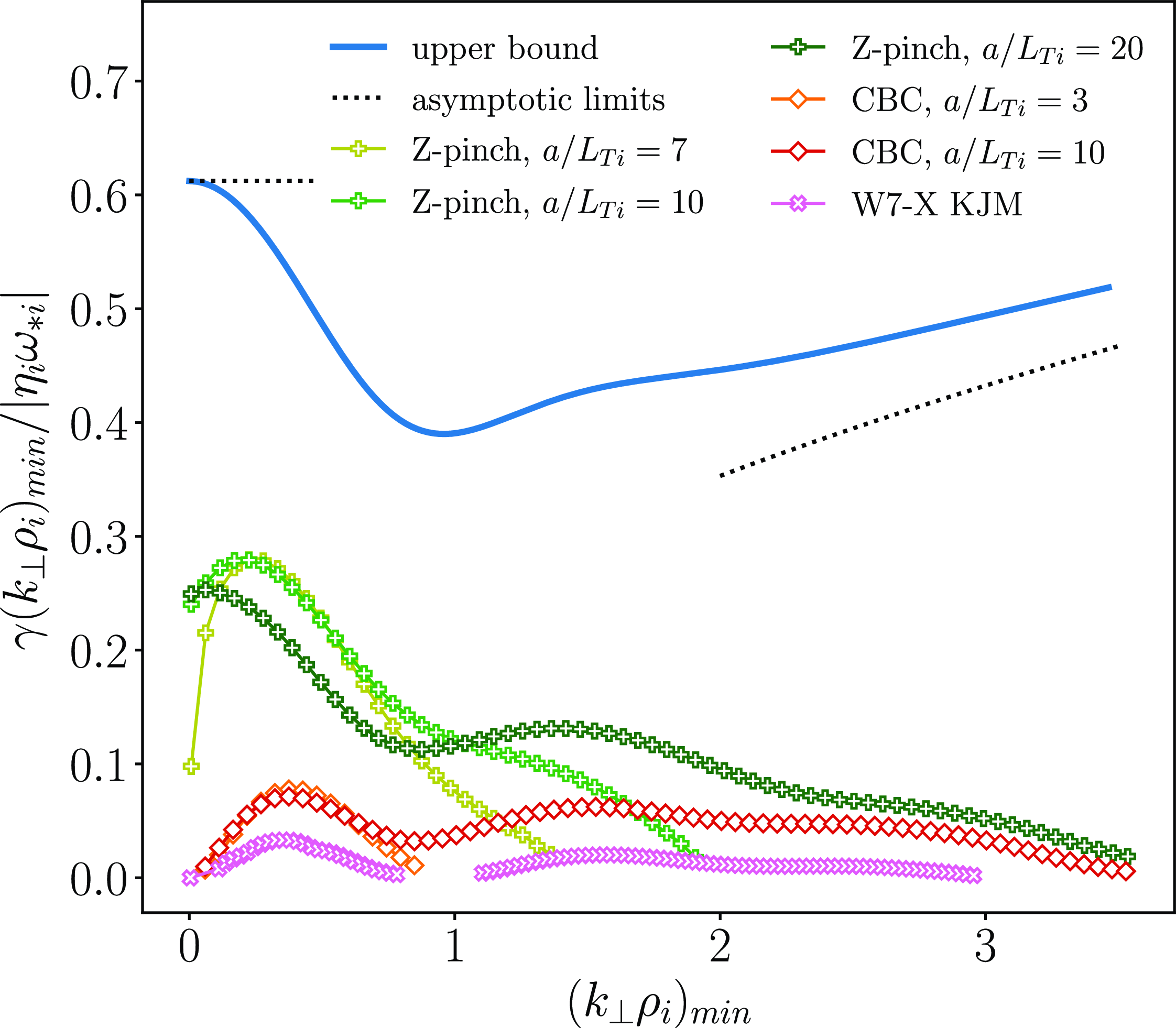
Figure 2. Upper bound for an electrostatic and collisionless hydrogen plasma with $\tau =1$
,
$\tau =1$
, $\nabla T_i\neq 0$
and kinetic electrons compared with results from gyrokinetic simulations. The W7-X simulation is obtained for
$\nabla T_i\neq 0$
and kinetic electrons compared with results from gyrokinetic simulations. The W7-X simulation is obtained for $a/L_{Ti}=3$
.
$a/L_{Ti}=3$
.
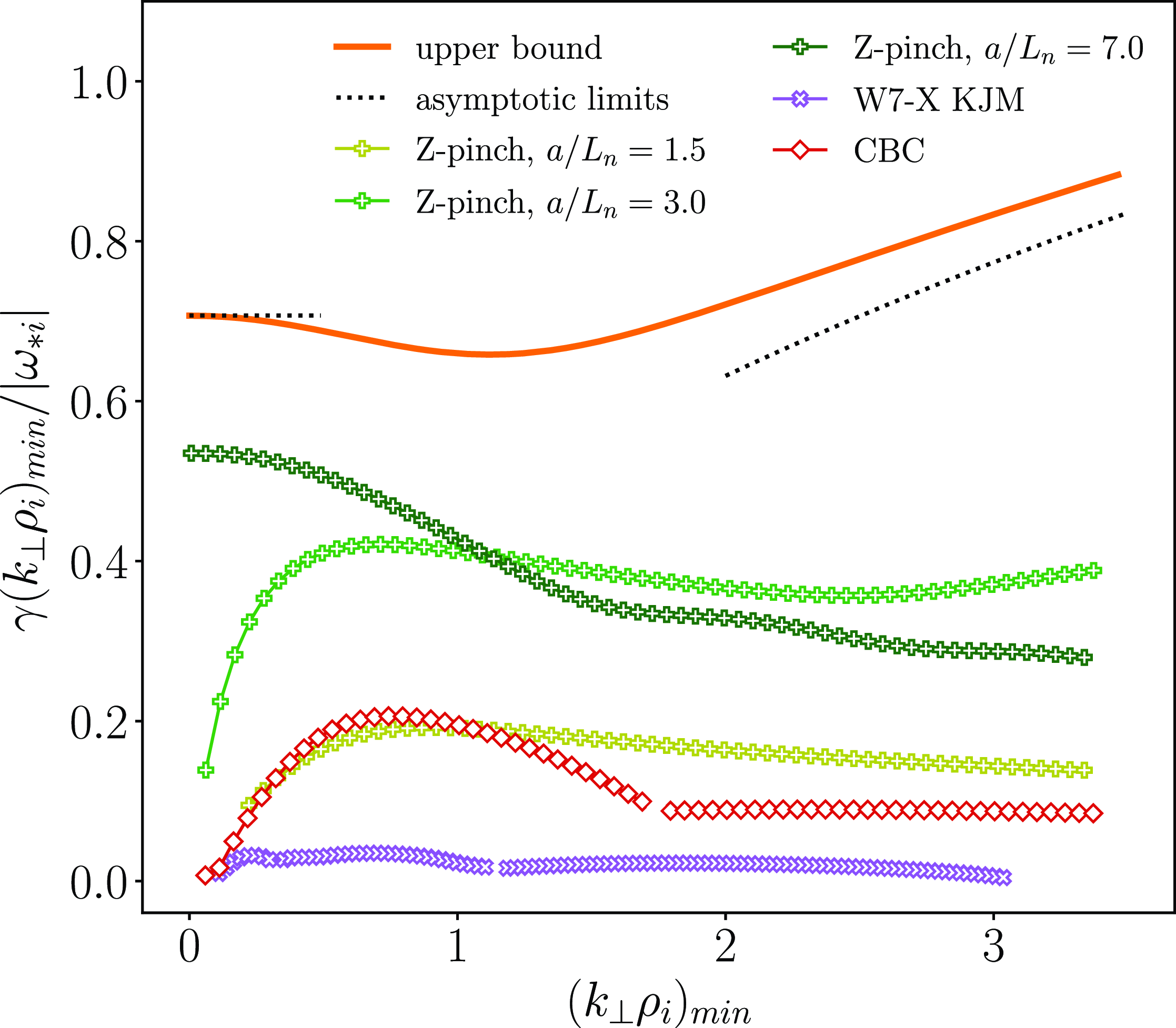
Figure 3. Upper bound for an electrostatic and collisionless hydrogen plasma with $\tau =1$
,
$\tau =1$
, $\nabla n\neq 0$
and kinetic electrons compared with results from gyrokinetic simulations. The W7-X and CBC simulations are obtained for
$\nabla n\neq 0$
and kinetic electrons compared with results from gyrokinetic simulations. The W7-X and CBC simulations are obtained for $a/L_n=3$
.
$a/L_n=3$
.
As noted in Part 2, this bound is not merely a generalisation of the single-kinetic-species ITG result. The two-species case can also describe magnetohydrodynamic interchange-like instabilities, which are present in closed-field-line geometries (Ricci et al. Reference Ricci, Rogers, Dorland and Barnes2006). These instabilities are characterised by a non-zero growth rate as $k_{\perp }\to 0$
, which explains why, at small wavenumbers, the upper bound approaches
$k_{\perp }\to 0$
, which explains why, at small wavenumbers, the upper bound approaches $\unicode{x1D6EC} (k_{\perp }\rho _i)_{\text{min}}/|\eta _i\omega _{*i}|=\sqrt {3/8}$
(2.20). The Z-pinch simulations confirm this behaviour, exhibiting a finite growth rate as
$\unicode{x1D6EC} (k_{\perp }\rho _i)_{\text{min}}/|\eta _i\omega _{*i}|=\sqrt {3/8}$
(2.20). The Z-pinch simulations confirm this behaviour, exhibiting a finite growth rate as $k_{\perp }\rho _i\to 0$
, especially as the ion temperature gradient increases.
$k_{\perp }\rho _i\to 0$
, especially as the ion temperature gradient increases.
As in the case of adiabatic electrons, we observe that the bound can predict the presence of both a primary and a secondary ITG maximum at approximately $(k_{\perp }\rho _i)_{\text{min}}\approx 0.5$
and
$(k_{\perp }\rho _i)_{\text{min}}\approx 0.5$
and $\approx 1.5$
, respectively. This behaviour is consistent across all the reported simulations, including those with Z-pinch, CBC and W7-X geometries. It is important to note that the absence of a SWITG mode in Z-pinch and CBC geometries in figure 1 can be attributed to the use of smaller gradients, resulting in a reduced drive. This is evident in figure 2, where the CBC spectrum at
$\approx 1.5$
, respectively. This behaviour is consistent across all the reported simulations, including those with Z-pinch, CBC and W7-X geometries. It is important to note that the absence of a SWITG mode in Z-pinch and CBC geometries in figure 1 can be attributed to the use of smaller gradients, resulting in a reduced drive. This is evident in figure 2, where the CBC spectrum at $a/L_{Ti}=10$
shows destabilisation at higher wavenumbers, while the spectrum at
$a/L_{Ti}=10$
shows destabilisation at higher wavenumbers, while the spectrum at $a/L_{Ti}=3$
does not. A similar trend is observed in W7-X.
$a/L_{Ti}=3$
does not. A similar trend is observed in W7-X.
For intermediate wavenumbers, the normalised upper bound behaves as $\sim \sqrt {(k_{\perp }\rho _i)_{\text{min}}}$
(2.21). At larger wavenumbers, we expect an inflection that causes the upper bound to stop increasing indefinitely and instead reach a saturation at a constant value. However, for the purposes of this article, we focus exclusively on ion-scale wavenumbers and therefore do not consider the upper bound behaviour at even larger wavenumbers. In general, the upper bound for two kinetic species is approximately four times higher than that for a single species. While this leads to a good qualitative agreement with the growth rates of normal modes, the quantitative match is less accurate, particularly for reactor-relevant geometries like the tokamak configuration of the CBC and the stellarator geometry of W7-X.
$\sim \sqrt {(k_{\perp }\rho _i)_{\text{min}}}$
(2.21). At larger wavenumbers, we expect an inflection that causes the upper bound to stop increasing indefinitely and instead reach a saturation at a constant value. However, for the purposes of this article, we focus exclusively on ion-scale wavenumbers and therefore do not consider the upper bound behaviour at even larger wavenumbers. In general, the upper bound for two kinetic species is approximately four times higher than that for a single species. While this leads to a good qualitative agreement with the growth rates of normal modes, the quantitative match is less accurate, particularly for reactor-relevant geometries like the tokamak configuration of the CBC and the stellarator geometry of W7-X.
Next, we perform a similar comparison, but with gradients $\nabla T_i=0$
and
$\nabla T_i=0$
and $\nabla n\neq 0$
, again including the Z-pinch, CBC and W7-X geometries in our analysis. For the Z-pinch configuration, we vary the normalised density gradient while keeping the other parameters fixed. We observe that, as in the previous cases, large density gradients drive instabilities with a non-zero growth rate for
$\nabla n\neq 0$
, again including the Z-pinch, CBC and W7-X geometries in our analysis. For the Z-pinch configuration, we vary the normalised density gradient while keeping the other parameters fixed. We observe that, as in the previous cases, large density gradients drive instabilities with a non-zero growth rate for $k_{\perp }\rho _i = 0$
. This behaviour is reflected in the upper bound, which tends to a constant for small wavenumbers. This constant value is given by (2.22) and is equal to
$k_{\perp }\rho _i = 0$
. This behaviour is reflected in the upper bound, which tends to a constant for small wavenumbers. This constant value is given by (2.22) and is equal to $\unicode{x1D6EC} (k_{\perp }\rho _i)_{\text{min}}/|\omega _{*i}|=\sqrt {1/2}$
for
$\unicode{x1D6EC} (k_{\perp }\rho _i)_{\text{min}}/|\omega _{*i}|=\sqrt {1/2}$
for $\tau =1$
.
$\tau =1$
.
For intermediate wavenumbers, the upper bound behaves like $\sim \sqrt {(k_{\perp }\rho _i)_{\text{min}}}$
, and we observe the same destabilisation of intermediate to large wavenumbers both in the Z-pinch and CBC geometries. As with the case of
$\sim \sqrt {(k_{\perp }\rho _i)_{\text{min}}}$
, and we observe the same destabilisation of intermediate to large wavenumbers both in the Z-pinch and CBC geometries. As with the case of $\nabla T_i\neq 0$
, we expect that the growth will not continue indefinitely, but will eventually saturate at a finite value for very large wavenumbers. However, our focus remains on ion-scale wavenumbers. As with the previous scenario, the W7-X curve is the furthest from the upper bound, while the Z-pinch with
$\nabla T_i\neq 0$
, we expect that the growth will not continue indefinitely, but will eventually saturate at a finite value for very large wavenumbers. However, our focus remains on ion-scale wavenumbers. As with the previous scenario, the W7-X curve is the furthest from the upper bound, while the Z-pinch with $a/L_n=7$
is the closest, with a ratio of
$a/L_n=7$
is the closest, with a ratio of ${\approx} 1.5$
.
${\approx} 1.5$
.
The characterisation of the instabilities in the CBC and W7-X simulations allows us to identify them as either trapped electron modes (TEMs) or ion-driven trapped electron modes (Plunk et al. Reference Plunk, Connor and Helander2017), depending on whether the real frequency of the instabilities aligns with the electron or ion diamagnetic direction, respectively. In W7-X, we also find universal instabilities for small values of the perpendicular wavenumber (Coppi & Pegoraro Reference Coppi and Pegoraro1977; Smolyakov et al. Reference Smolyakov, Yagi and Kishimoto2002b ; Landreman et al. Reference Landreman, Antonsen and Dorland2015a ; Helander & Plunk Reference Helander and Plunk2015; Costello et al. Reference Costello, Proll, Plunk, Pueschel and Alcusón2023; Podavini et al. Reference Podavini, Zocco, García-Regaña, Barnes, Parra, Mishchenko and Helander2024). The characterisation required the inspection of the real frequency sign (see figure 13 in Appendix B) and the parallel structure of the eigenfunctions along the magnetic field lines.
5. How optimal are normal modes?
In the previous section, we contrasted optimal-mode theory with normal-mode theory by comparing growth rates across different geometries and plasma parameters. We observed that, while the upper bound often provides a qualitative match with the growth rates, it falls short of being a quantitative match in many cases. This discrepancy arises from the different types of modes with which the upper bound and growth rates are associated. As previously mentioned, optimal modes are not conventional eigenmodes; they represent the system’s instantaneous response to a localised injection of free energy. In contrast, normal modes describe exponentially growing, or damped, instabilities with a defined structure along magnetic field lines. Consequently, optimal modes and normal modes can have very different mathematical forms, and we do not expect them to coincide. However, we can explore how closely they approach each other by exploiting the completeness and orthogonality of the optimal modes.
In particular, considering the vector $\mathbf{g}$
, with components
$\mathbf{g}$
, with components $g_a$
, the inner product between two vectors
$g_a$
, the inner product between two vectors $\mathbf{g_1}$
and
$\mathbf{g_1}$
and $\mathbf{g_2}$
is given by
$\mathbf{g_2}$
is given by
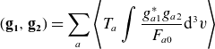 \begin{equation} (\mathbf{g_1}, \mathbf{g_2} )=\sum _a\Bigg \langle T_a\int \frac {g_{a1}^*g_{a2}}{F_{a0}}\text{d}^{3}v\Bigg \rangle \end{equation}
and the free energy balance equation (2.6) can be rewritten in inner product notation as
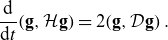 \begin{equation} \frac {\mathrm{d}}{\mathrm{d} t}(\mathbf{g},\mathcal{H}\mathbf{g})=2(\mathbf{g},\mathcal{D}\mathbf{g})\; . \end{equation}
The state $\mathbf{g}$
can be expanded by taking into consideration the completeness of optimal modes,
$\mathbf{g}$
can be expanded by taking into consideration the completeness of optimal modes,
 \begin{equation} \mathbf{g}=\sum _n c_n\mathbf{g}_n\; . \end{equation}
It follows that
 \begin{equation} \begin{split} (\mathbf{g},\mathcal{H}\mathbf{g}_n)=&\sum _m c_m(\mathbf{g}_m,\mathcal{H}\mathbf{g}_n)\\ =&\ c_n(\mathbf{g}_n,\mathcal{H}\mathbf{g}_n)\\ =&\ c_n||\mathbf{g}_n||^2, \end{split} \end{equation}
where we used the orthogonality property (Plunk & Helander Reference Plunk and Helander2022) $(\mathbf{g}_m,\mathcal{H}\mathbf{g}_n)=\delta _{mn}||\mathbf{g}_n||^2$
, defining
$(\mathbf{g}_m,\mathcal{H}\mathbf{g}_n)=\delta _{mn}||\mathbf{g}_n||^2$
, defining $||\mathbf{g}_n||^2\equiv (\mathbf{g}_n,\mathcal{H}\mathbf{g}_n)$
. The coefficients of the expansion are thus given by
$||\mathbf{g}_n||^2\equiv (\mathbf{g}_n,\mathcal{H}\mathbf{g}_n)$
. The coefficients of the expansion are thus given by $c_n = (\mathbf{g},\mathcal{H}\mathbf{g}_n)/||\mathbf{g}_n||^2$
.
$c_n = (\mathbf{g},\mathcal{H}\mathbf{g}_n)/||\mathbf{g}_n||^2$
.
For this study, we decide to focus on the ITG scenario with adiabatic electrons for two reasons: first, because of the promising results obtained for the comparison shown in figure 1 and second, since the ITG instability can be analytically described in certain limits, as outlined in § 3.
We consider the non-adiabatic part of the distribution function for the ions, denoted as $g_i$
, and expand it using the appropriate optimal modes basis (2.11). To simplify the analysis, we focus on the small Larmor radius scenario, for which the optimal modes are
$g_i$
, and expand it using the appropriate optimal modes basis (2.11). To simplify the analysis, we focus on the small Larmor radius scenario, for which the optimal modes are
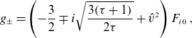 \begin{equation} g_{\pm }=\left (-\frac {3}{2}\mp i\sqrt {\frac {3(\tau +1)}{2\tau }}+\hat {v}^2\right )F_{i0}\; , \end{equation}
where $g_+$
is associated with instantaneous growth and
$g_+$
is associated with instantaneous growth and $g_-$
with instantaneous damping. In this case, the
$g_-$
with instantaneous damping. In this case, the $\mathcal{H}$
operator is defined as follows:
$\mathcal{H}$
operator is defined as follows:
 \begin{equation} \mathcal{H}g=g-\frac {F_0}{n(1+\tau )}\int g(\boldsymbol{v}')\text{d}^{3}v'\; . \end{equation}
Following (5.3), we write
 \begin{equation} g_{i}=c_+g_+ + c_-g_- + g_0\; , \end{equation}
where $g_0$
represents the contribution lying in the null space of the
$g_0$
represents the contribution lying in the null space of the $\mathcal{D}$
operator, which is populated by modes that do not increase nor decrease the Helmholtz free energy associated with
$\mathcal{D}$
operator, which is populated by modes that do not increase nor decrease the Helmholtz free energy associated with $g_i$
.
$g_i$
.
We then use the orthogonality of the optimal modes to calculate the fractions that represent the relative contribution of each optimal mode to the ITG eigenmode. These fractions collectively sum to unity,
 \begin{equation} f_+ + f_- + f_0 = 1, \end{equation}
where
 \begin{equation} \begin{gathered} f_\pm =|c_\pm |^2||g_\pm ||^2/||g_i||^2=|(g_i,\mathcal{H}g_\pm )|^2/||g_i||^2\\ f_0 = ||g_0||^2/||g_i||^2\; . \end{gathered} \end{equation}
The contributions from each optimal mode vary depending on the parameters on which both $g_i$
and the optimal modes depend. Specifically, the optimal modes are solely a function of
$g_i$
and the optimal modes depend. Specifically, the optimal modes are solely a function of $\tau$
(as shown in (5.5)), while
$\tau$
(as shown in (5.5)), while $g_i$
depends on
$g_i$
depends on $\tau$
but also on the diamagnetic frequency
$\tau$
but also on the diamagnetic frequency $\omega _{*i}$
and, if the mode is toroidal-like (3.5), on the drift frequency
$\omega _{*i}$
and, if the mode is toroidal-like (3.5), on the drift frequency $\omega _{\kappa i}$
. For slab-like modes (3.1),
$\omega _{\kappa i}$
. For slab-like modes (3.1), $g_i$
depends on the parallel transit frequency
$g_i$
depends on the parallel transit frequency $\omega _{\parallel }$
. Therefore, we conduct a parameter scan to analyse the trends in these different contributions.
$\omega _{\parallel }$
. Therefore, we conduct a parameter scan to analyse the trends in these different contributions.
To begin, we assume $g_i$
describes a strongly driven toroidal ITG mode. Under this assumption, the resonant denominator in (3.5) can be expanded and the mode frequency
$g_i$
describes a strongly driven toroidal ITG mode. Under this assumption, the resonant denominator in (3.5) can be expanded and the mode frequency $\omega$
is given by (3.9). We further simplify the analysis by considering flat density profiles, setting
$\omega$
is given by (3.9). We further simplify the analysis by considering flat density profiles, setting $\omega _{*i}=0$
, while keeping
$\omega _{*i}=0$
, while keeping $\eta _i\omega _{*i}\equiv \omega _{*i}^t\neq 0$
. We then produce three different maps illustrating the contributions
$\eta _i\omega _{*i}\equiv \omega _{*i}^t\neq 0$
. We then produce three different maps illustrating the contributions $f_+$
,
$f_+$
, $f_-$
and
$f_-$
and $f_0$
for various values of
$f_0$
for various values of $\tau$
and the ratio
$\tau$
and the ratio $2\omega _{*i}^t/\omega _{\kappa i}=a/L_{Ti}$
. These maps are shown in figure 4.
$2\omega _{*i}^t/\omega _{\kappa i}=a/L_{Ti}$
. These maps are shown in figure 4.
In these maps, two distinct regions are outlined by the marginality (linear stability threshold) contour. The solid orange line indicates marginality calculated using the strongly driven toroidal ITG dispersion relation of (3.9), whereas the red dashed curve represents the exact marginality contour derived from the small Larmor radius dispersion relation of (3.8). The coincidence of the two contours in the limit $\tau \to 0$
suggests that, in this regime, the mode behaves as in the fluid approximation, even approaching the point of marginal stability.
$\tau \to 0$
suggests that, in this regime, the mode behaves as in the fluid approximation, even approaching the point of marginal stability.
The unstable region lies to the right of the marginality curve, and within this region, we expect that $f_+\gt f_-$
. This follows from
$f_+\gt f_-$
. This follows from
 \begin{equation} 2\gamma = \frac {\mathrm{d}}{\mathrm{d} t}||g_i||^2/||g_i||^2=2\unicode{x1D6EC} _+(f_+-f_-)\; , \end{equation}
which we derived starting from (5.2), whose right-hand side has been evaluated by using (5.3) and (2.18). Moreover, we used $\unicode{x1D6EC} _-=-\unicode{x1D6EC} _+$
, as evident from (2.14).
$\unicode{x1D6EC} _-=-\unicode{x1D6EC} _+$
, as evident from (2.14).
The results shown in figure 4 agree with our expectations. In the region to the right of the marginality contour, where instability is expected, we indeed observe that $f_+\gt f_-$
. The maximum projection onto the growing optimal mode occurs at the parameter set
$f_+\gt f_-$
. The maximum projection onto the growing optimal mode occurs at the parameter set $\{2\omega _{*i}^t/\omega _{\kappa i},\tau \}=\{3,0.3\}$
, where
$\{2\omega _{*i}^t/\omega _{\kappa i},\tau \}=\{3,0.3\}$
, where $f_+$
reaches a value of approximately
$f_+$
reaches a value of approximately $0.75$
. Conversely, for this same parameter set, the projection onto the damped optimal mode
$0.75$
. Conversely, for this same parameter set, the projection onto the damped optimal mode $f_-$
reaches its minimum. The projection onto the null space
$f_-$
reaches its minimum. The projection onto the null space $f_0$
is very small across almost the entire map.
$f_0$
is very small across almost the entire map.

Figure 4. Projections of the strongly driven toroidal ITG mode onto the optimal modes basis for an electrostatic hydrogen plasma with adiabatic electrons. The solid orange line indicates marginality for the strongly driven ITG (3.9), while the dashed red curve indicates marginality as calculated by solving the small Larmor radius dispersion relation (3.8). The definitions of $f_+$
,
$f_+$
, $f_-$
and
$f_-$
and $f_0$
are reported in (5.9).
$f_0$
are reported in (5.9).
As $\omega _{*i}^t/\tau$
increases, corresponding to the region where the fluid approximation is valid, both
$\omega _{*i}^t/\tau$
increases, corresponding to the region where the fluid approximation is valid, both $f_+$
and
$f_+$
and $f_-$
tend towards a value of approximately
$f_-$
tend towards a value of approximately $0.5$
, with
$0.5$
, with $f_+$
approaching from above and
$f_+$
approaching from above and $f_-$
from below. According to (5.10), this indicates that the ratio
$f_-$
from below. According to (5.10), this indicates that the ratio $\gamma /\unicode{x1D6EC} _+$
approaches zero. Consequently, in the fluid limit, the upper bound is furthest from the normal-mode growth rate. Indeed, while the fluid-ITG growth rate scales as
$\gamma /\unicode{x1D6EC} _+$
approaches zero. Consequently, in the fluid limit, the upper bound is furthest from the normal-mode growth rate. Indeed, while the fluid-ITG growth rate scales as $\sqrt {\omega _{\kappa i}\omega _{*i}^t/\tau }$
(3.9), the upper bound scales as
$\sqrt {\omega _{\kappa i}\omega _{*i}^t/\tau }$
(3.9), the upper bound scales as $\sim \omega _{*i}^t/\tau$
(2.14), causing their ratio to decrease as the temperature gradient increases or
$\sim \omega _{*i}^t/\tau$
(2.14), causing their ratio to decrease as the temperature gradient increases or $\tau$
decreases.
$\tau$
decreases.
On the fluid marginality contour, i.e. for $\tau \ll 1$
,
$\tau \ll 1$
, $f_+=f_-$
and thus
$f_+=f_-$
and thus $f_+-f_-=0$
, once again indicating that the fluid approximation correctly describes this region. In contrast, it is important to note that the fluid approximation used does not accurately describe the stability threshold for
$f_+-f_-=0$
, once again indicating that the fluid approximation correctly describes this region. In contrast, it is important to note that the fluid approximation used does not accurately describe the stability threshold for $\tau \gtrsim 1$
, where kinetic effects become dominant. We expect neither the strongly driven toroidal ITG eigenmode nor the optimal modes to reliably capture the stability threshold there. Consequently, the projections in the region near the kinetic marginality contour should be interpreted with this in mind.
$\tau \gtrsim 1$
, where kinetic effects become dominant. We expect neither the strongly driven toroidal ITG eigenmode nor the optimal modes to reliably capture the stability threshold there. Consequently, the projections in the region near the kinetic marginality contour should be interpreted with this in mind.
To also accurately describe marginality for $\tau \gtrsim 1$
, we use the full kinetic toroidal ITG distribution function (3.5) and substitute
$\tau \gtrsim 1$
, we use the full kinetic toroidal ITG distribution function (3.5) and substitute $\omega$
derived from numerically solving the small Larmor radius dispersion relation of Biglari et al. Reference Biglari, Diamond and Rosenbluth(1989) (3.8), while considering
$\omega$
derived from numerically solving the small Larmor radius dispersion relation of Biglari et al. Reference Biglari, Diamond and Rosenbluth(1989) (3.8), while considering $\omega _{*i}=0$
and
$\omega _{*i}=0$
and $\omega _{*i}^t\neq 0$
.
$\omega _{*i}^t\neq 0$
.
The results are presented in figure 5. At marginality, the projections align with the expectations from (5.10). Specifically, along the kinetic marginality contour, both $f_+$
and
$f_+$
and $f_-$
, as well as their difference
$f_-$
, as well as their difference $f_+-f_-$
, approach values close to zero. In the same region,
$f_+-f_-$
, approach values close to zero. In the same region, $f_0$
attains larger values, indicating that the null space – which neither contributes to the mode’s growth nor its damping – becomes increasingly significant in this part of the parameter space.
$f_0$
attains larger values, indicating that the null space – which neither contributes to the mode’s growth nor its damping – becomes increasingly significant in this part of the parameter space.
Figure 5. Projections of the drift-kinetic toroidal ITG mode onto the optimal modes basis for an electrostatic hydrogen plasma with adiabatic electrons. The solid orange line indicates marginality for the strongly driven ITG (3.9), while the dashed red curve indicates marginality as calculated by solving the small Larmor radius dispersion relation (3.8). The definitions of $f_+$
,
$f_+$
, $f_-$
and
$f_-$
and $f_0$
are reported in (5.9).
$f_0$
are reported in (5.9).
Crossing the kinetic marginality contour from left to right, we go from a region where $f_+\lt f_-$
, and thus where the mode is damped, to a region where
$f_+\lt f_-$
, and thus where the mode is damped, to a region where $f_+\gt f_-$
, and thus where the instability is present. The maximum of the projection onto the growing optimal mode is reached along the
$f_+\gt f_-$
, and thus where the instability is present. The maximum of the projection onto the growing optimal mode is reached along the $10\tau \approx 2\omega _{*i}^t/\omega _{\kappa i}$
contour. Specifically, the global maximum is reached for
$10\tau \approx 2\omega _{*i}^t/\omega _{\kappa i}$
contour. Specifically, the global maximum is reached for $\{2\omega _{*i}^t/\omega _{\kappa i},\tau \}=\{10,0.3\}$
, where
$\{2\omega _{*i}^t/\omega _{\kappa i},\tau \}=\{10,0.3\}$
, where $f_+$
reaches a value of approximately
$f_+$
reaches a value of approximately $0.76$
. This contour reflects the toroidal ITG resonance condition of Biglari et al. Reference Biglari, Diamond and Rosenbluth(1989) found for
$0.76$
. This contour reflects the toroidal ITG resonance condition of Biglari et al. Reference Biglari, Diamond and Rosenbluth(1989) found for $\omega _{*i}^t\sim \omega _{\kappa i}$
and suggests that the resonance is important to approach optimal behaviour. In the region where
$\omega _{*i}^t\sim \omega _{\kappa i}$
and suggests that the resonance is important to approach optimal behaviour. In the region where $\omega _{*i}^t/\tau$
is large, both
$\omega _{*i}^t/\tau$
is large, both $f_+$
and
$f_+$
and $f_-$
approach 0.5, with
$f_-$
approach 0.5, with $f_+$
taking values slightly larger than 0.5 and
$f_+$
taking values slightly larger than 0.5 and $f_-$
slightly smaller. This confirms that the strongly driven dispersion relation, as given by (3.9), is appropriate for this limit.
$f_-$
slightly smaller. This confirms that the strongly driven dispersion relation, as given by (3.9), is appropriate for this limit.
We conclude that the drift-kinetic toroidal ITG mode is up to approximately 80 % composed of an instantaneously growing optimal mode, and this proportion is attained in the neighbourhood of the stability threshold, indicating that resonance effects are influential. However, this behaviour is observed only when the threshold is resonant ( $\tau \gtrsim 1$
). In contrast, near the threshold described by a fluid approximation (
$\tau \gtrsim 1$
). In contrast, near the threshold described by a fluid approximation ( $\tau \ll 1$
), this proportion is not observed. The fluid-like toroidal ITG, which is found at
$\tau \ll 1$
), this proportion is not observed. The fluid-like toroidal ITG, which is found at $\tau \ll 2\omega _{*i}^t/\omega _{\kappa i}$
, is composed to 50 % by an optimal growing mode and to 50 % by a damped one, with the former having the upper hand in the sense that an instability indeed occurs.
$\tau \ll 2\omega _{*i}^t/\omega _{\kappa i}$
, is composed to 50 % by an optimal growing mode and to 50 % by a damped one, with the former having the upper hand in the sense that an instability indeed occurs.
As already observed for the projections derived assuming a fluid approximation for $g_i$
(figure 4), this brings to an unfavourable scaling of the ratio
$g_i$
(figure 4), this brings to an unfavourable scaling of the ratio $\gamma /\unicode{x1D6EC} _+$
with
$\gamma /\unicode{x1D6EC} _+$
with $\omega _{*i}^t/\tau$
. It is shown in Part 3 (Plunk & Helander Reference Plunk and Helander2023) and Part 4 (Costello & Plunk Reference Costello and Plunk2025) that a more favourable trend of the toroidal ITG normal-mode and upper bound ratio is achievable through the definition of a generalised free energy.
$\omega _{*i}^t/\tau$
. It is shown in Part 3 (Plunk & Helander Reference Plunk and Helander2023) and Part 4 (Costello & Plunk Reference Costello and Plunk2025) that a more favourable trend of the toroidal ITG normal-mode and upper bound ratio is achievable through the definition of a generalised free energy.
The area to the left of the marginality contour encompasses a region where the ITG eigenmode is stabilised and only damped solutions exist. Consequently, we omit the analysis of the projections in this area.
6. Conclusions
In this work, we have compared the conventional normal-mode approach to gyrokinetic instabilities with the recently developed optimal-mode approach (Helander & Plunk Reference Helander and Plunk2021; Plunk & Helander Reference Plunk and Helander2022). We have considered three separate cases of two gyrokinetic instabilities relevant to fusion magnetic confinement devices, the ion temperature gradient (ITG) mode and the density-gradient-driven trapped electron modes (TEMs). A range of magnetic geometries were considered, including tokamak, stellarator, Z-pinch and slab plasmas.
All the cases considered showed that the growth rates of normal modes consistently remain below the upper bounds across various geometries and temperature or density gradients. This result was anticipated, as the derivation of the upper bounds is based on thermodynamic principles and involves no approximations.
The upper bounds are sometimes several times higher than the normal-mode growth rates, especially for tokamaks and stellarators. This discrepancy stems from the fact that the sources of Helmholtz free energy are independent of the magnetic geometry. As a result, the upper bounds studied here do not incorporate the geometric effects and resonance mechanisms that affect the stability properties of different magnetic confinement devices.
However, we also observe that the upper bounds, somewhat unexpectedly, replicate key features of the growth-rate spectra. For instance, they capture the behaviour at small and intermediate wavenumbers, relative to ion scales, and surprisingly accurately indicate the positions of the fastest-growing modes for both the conventional ITG and short-wavelength ITG instabilities. These observations underscore the qualitative utility of the upper bounds in describing key characteristics of gyrokinetic instabilities, even if they do not precisely match the growth rates.
For improved quantitative agreement, optimal mode theory is being extended to include information about the magnetic geometry, as well as physics of wave–particle resonances. These extensions could enable the development of quasi-linear models, offering an alternative to existing approaches based on normal modes.
Conceptually, normal modes and optimal modes are distinct mathematical objects, as discussed in §§ 2 and 3. To quantify the difference between these two types of modes, we have measured the distance between them by projecting normal modes – specifically for a toroidal ITG mode with adiabatic electron response – onto the optimal modes basis across a wide range of parameters. For the cases studied, our analysis demonstrated that the decomposition of an ITG mode has at most a 80 % contribution from the instantaneously growing optimal mode, achieved in the resonant limit. This emphasises the difference between optimal mode theory and fluid theory, a common approximation for instabilities, which fails in the resonant limit. It also explains why we do not observe, nor should expect, the growth rates of normal modes to exactly coincide with the upper bounds derived from Helmholtz free energy.
Acknowledgements
The authors would like to thank P. Costello for the fruitful discussions and A. Hallenbert for the GENE simulations. The stella simulations were performed on the Raven HPC (MPCDF, Germany).
Editor Paolo Ricci thanks the referees for their advice in evaluating this article.
Funding
This work has been carried out within the framework of the EUROfusion Consortium, via the Euratom Research and Training Programme (Grant Agreement No 101052200 – EUROfusion). Views and opinions expressed are however those of the author(s) only and do not necessarily reflect those of the European Union or the European Commission. Neither the European Union nor the European Commission can be held responsible for them.
Declaration of interests
The authors report no conflict of interest.
Appendix A. Numerical validation of toroidal ITG dispersion relation and Z-pinch geometry implementation
In this appendix, we assess the range of validity of the dispersion relations reported in § 3. To do so, we solve the gyrokinetic equation (2.1) using stella , by implementing a purely toroidal magnetic field, referred to as Z-pinch geometry. We further validate the dispersion relations and the stella Z-pinch geometry implementation by comparing the results with simulations performed with the gyrokinetic code GENE (Jenko et al. Reference Jenko, Dorland, Kotschenreuther and Rogers2000). Our Z-pinch geometry implementation is indeed based on previous work conducted with the GENE code (Navarro et al. Reference Navarro, Teaca and Jenko2016).
The Z-pinch geometry is achieved by mapping the cylindrical coordinates $(\tilde {r},\tilde {\theta },\tilde {z})$
to stella coordinates
$(\tilde {r},\tilde {\theta },\tilde {z})$
to stella coordinates $(x,y,z)$
. The magnetic field lines are described by the field-following coordinate
$(x,y,z)$
. The magnetic field lines are described by the field-following coordinate $z=\tilde {\theta }\equiv \hat {\mathbf{b}}$
, which, along with the
$z=\tilde {\theta }\equiv \hat {\mathbf{b}}$
, which, along with the $y$
coordinate, parametrises the flux surfaces. The chosen flux surface is identified with the cylinder’s radius
$y$
coordinate, parametrises the flux surfaces. The chosen flux surface is identified with the cylinder’s radius $\tilde {r}=R$
. The coordinate
$\tilde {r}=R$
. The coordinate $x$
is thus perpendicular to the flux surfaces, while
$x$
is thus perpendicular to the flux surfaces, while $y$
maps the direction of the current
$y$
maps the direction of the current $\mathbf{I}$
that produces the magnetic field
$\mathbf{I}$
that produces the magnetic field $\mathbf{B}$
, as illustrated in figure 6. Together,
$\mathbf{B}$
, as illustrated in figure 6. Together, $x$
and
$x$
and $y$
describe the plane perpendicular to magnetic field lines. It follows that the magnetic field magnitude is described by
$y$
describe the plane perpendicular to magnetic field lines. It follows that the magnetic field magnitude is described by $B(x)=2I/cx$
, and the metric coefficients that enter in the gyrokinetic equation are
$B(x)=2I/cx$
, and the metric coefficients that enter in the gyrokinetic equation are $g^{xx}=g^{yy}=g^{zz}=1$
,
$g^{xx}=g^{yy}=g^{zz}=1$
, $g^{xy}=g^{xz}=g^{yz}=0$
. The scale length of the magnetic field variation,
$g^{xy}=g^{xz}=g^{yz}=0$
. The scale length of the magnetic field variation, $L_B$
, is determined by its radial derivative and coincides with the cylinder radius
$L_B$
, is determined by its radial derivative and coincides with the cylinder radius
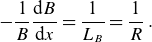 \begin{equation} -\frac {1}{B}\frac {\mathrm{d} B}{\mathrm{d}x}=\frac {1}{L_{B}}=\frac {1}{R}\; . \end{equation}
The scale length $L_B$
is used to normalise all other scale lengths and to keep a consistent notation with § 4, it is hereafter defined as
$L_B$
is used to normalise all other scale lengths and to keep a consistent notation with § 4, it is hereafter defined as $a$
. The
$a$
. The $\nabla y$
component of the magnetic drift,
$\nabla y$
component of the magnetic drift, $(\hat {\mathbf{b}}\times \mathbf{\kappa })\cdot \nabla y=(\hat {\mathbf{b}}\times \nabla B)\cdot \nabla y$
, is proportional to the radial derivative of the magnetic field and is therefore constant along the field line. There is no magnetic drift in the
$(\hat {\mathbf{b}}\times \mathbf{\kappa })\cdot \nabla y=(\hat {\mathbf{b}}\times \nabla B)\cdot \nabla y$
, is proportional to the radial derivative of the magnetic field and is therefore constant along the field line. There is no magnetic drift in the $x$
-direction.
$x$
-direction.

Figure 6. Sketch of the cylindrical Z-pinch flux-surface parametrised by the coordinates implemented in stella . Drawing adapted from Ivanov et al. Reference Ivanov, Schekochihin, Dorland, Field and Parra(2020).
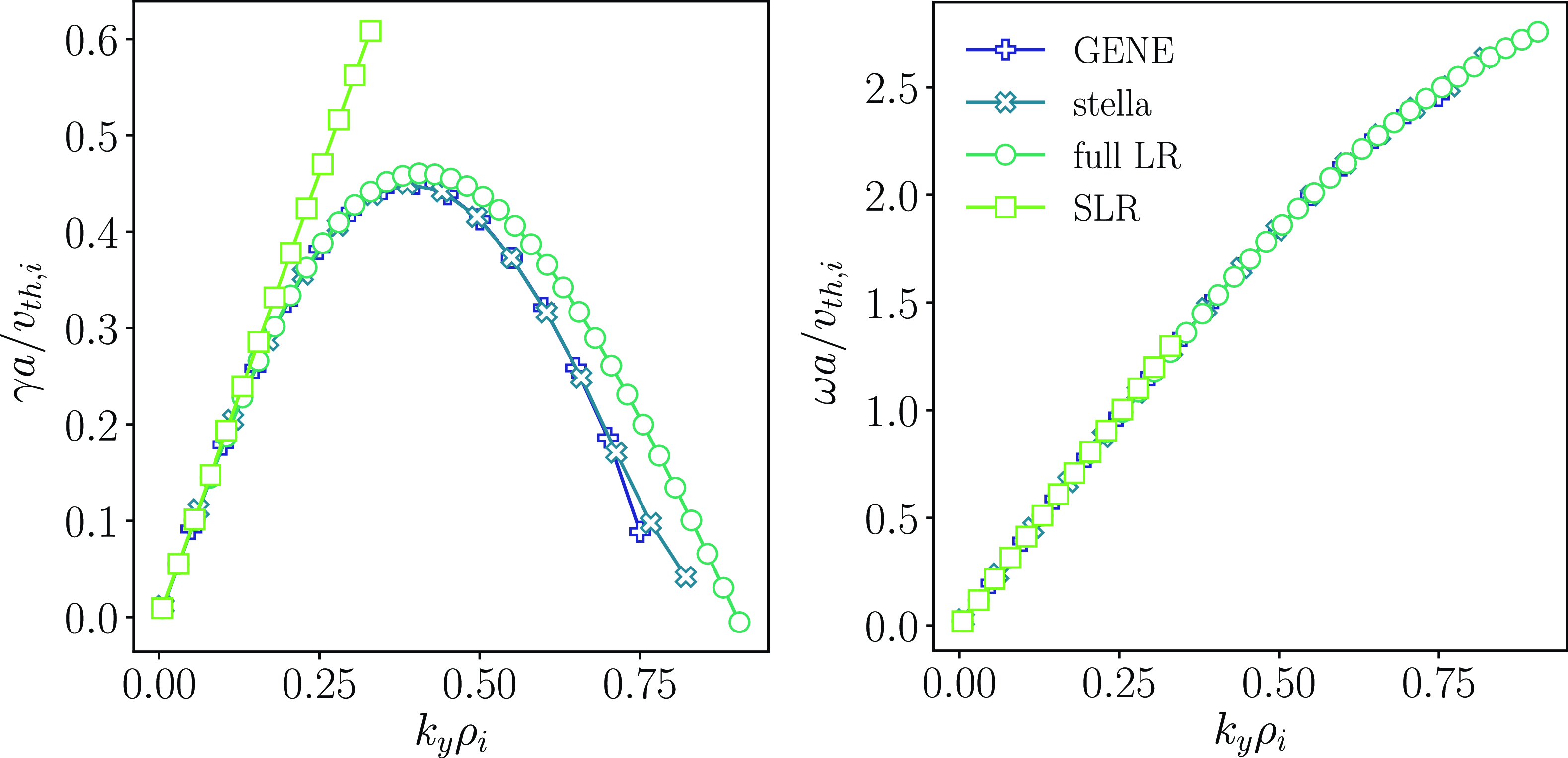
Figure 7. Normalised growth rate $\gamma a/v_{th,i}$
and real frequency
$\gamma a/v_{th,i}$
and real frequency $\omega a/v_{th,i}$
for Z-pinch geometry simulations performed for
$\omega a/v_{th,i}$
for Z-pinch geometry simulations performed for $a/L_{Ti}=6.4$
with the gyrokinetic codes GENE and
stella
, compared with solutions of the full Larmor radius (full LR) resonant dispersion relation – (3.6) – and the small Larmor radius (SLR) one – (3.8).
$a/L_{Ti}=6.4$
with the gyrokinetic codes GENE and
stella
, compared with solutions of the full Larmor radius (full LR) resonant dispersion relation – (3.6) – and the small Larmor radius (SLR) one – (3.8).
To validate the local theories described in § 3, we perform electrostatic, collisionless flux-tube simulations while neglecting the parallel streaming term in (2.1). We simulate a single ion kinetic species and set $\tau =T_i/T_e=1$
. Our initial comparison focuses on the dispersion relations for a fixed value of the normalised ion temperature gradient
$\tau =T_i/T_e=1$
. Our initial comparison focuses on the dispersion relations for a fixed value of the normalised ion temperature gradient $a/L_{Ti}=6.4$
. We set a flat density profile.
$a/L_{Ti}=6.4$
. We set a flat density profile.
In figure 7, we compare the outcomes from GENE and stella simulations with the roots of the resonant dispersion relation that includes full Larmor radius effects (full LR – (3.6)) and of the small Larmor radius one (SLR – (3.8)). The comparison shows excellent agreement both between the two codes and the full LR dispersion relation.Footnote
2
As anticipated, the SLR dispersion relation provides a good approximation of both the numerical results and the analytical full LR dispersion relation only for $k_y\rho _i\to 0$
. In this regime, the growth rate shows a linear behaviour with
$k_y\rho _i\to 0$
. In this regime, the growth rate shows a linear behaviour with $k_y\rho _i$
, as expected for a strongly driven toroidal ITG (3.9).
$k_y\rho _i$
, as expected for a strongly driven toroidal ITG (3.9).
We perform additional benchmark cases for various normalised temperature gradients: in figure 8, we show the one for $a/L_{Ti}=3.7$
and in figure 9, the one for
$a/L_{Ti}=3.7$
and in figure 9, the one for $a/L_{Ti}=12.8$
. For the case with
$a/L_{Ti}=12.8$
. For the case with $a/L_{Ti}=3.7$
, we once again observe excellent agreement between the growth rate and the frequency, both when comparing the two different numerical results and when comparing the numerical results with the full LR dispersion relation. At small wavenumbers, the agreement with the SLR dispersion relation is also perfect, further validating the accuracy of the SLR approximation in this regime.
$a/L_{Ti}=3.7$
, we once again observe excellent agreement between the growth rate and the frequency, both when comparing the two different numerical results and when comparing the numerical results with the full LR dispersion relation. At small wavenumbers, the agreement with the SLR dispersion relation is also perfect, further validating the accuracy of the SLR approximation in this regime.
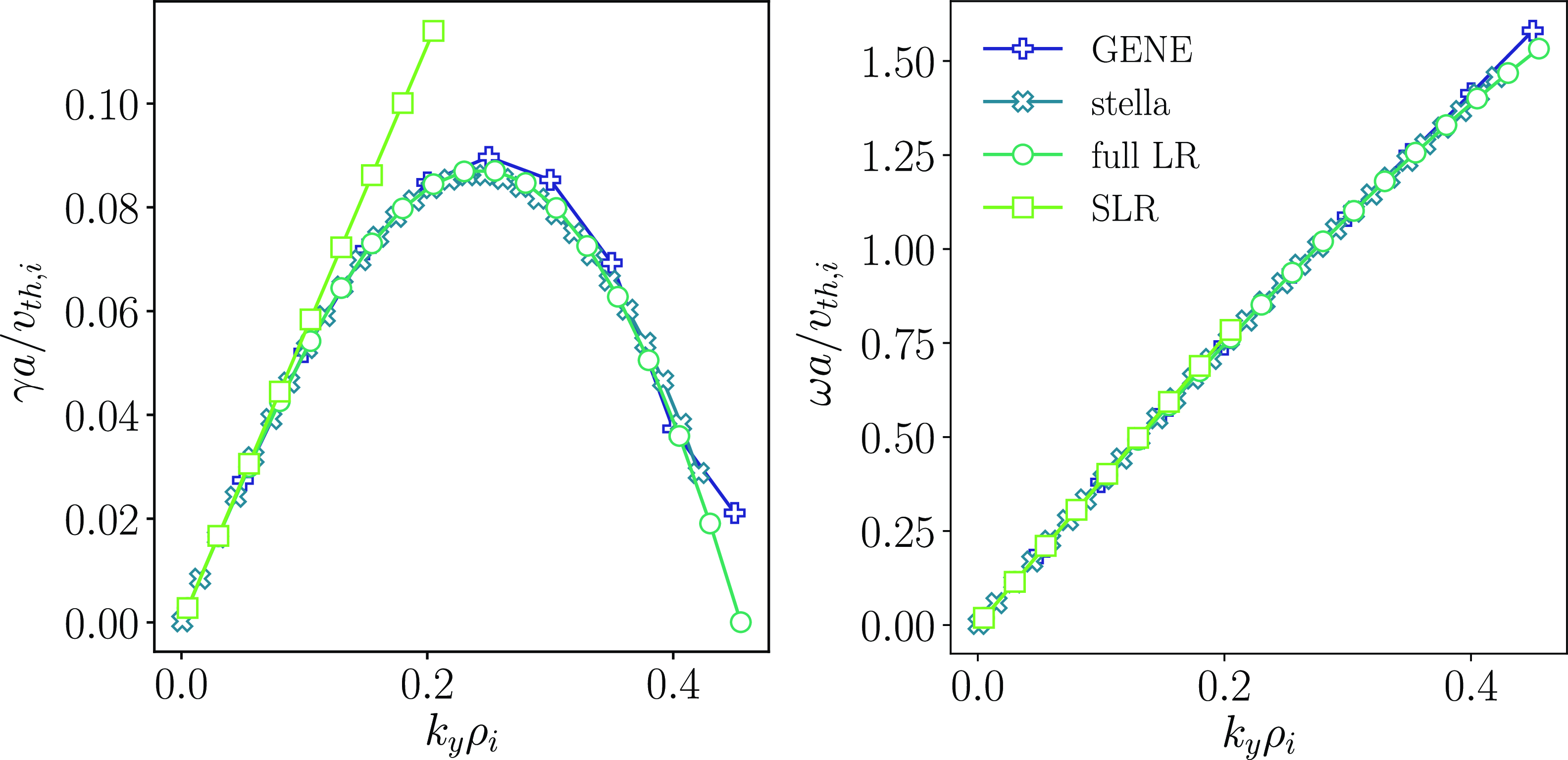
Figure 8. Normalised growth rate $\gamma a/v_{th,i}$
and real frequency
$\gamma a/v_{th,i}$
and real frequency $\omega a/v_{th,i}$
for Z-pinch geometry simulations performed for
$\omega a/v_{th,i}$
for Z-pinch geometry simulations performed for $a/L_{Ti}=3.7$
with the gyrokinetic codes GENE and
stella
, compared with solutions of the full Larmor radius (full LR) resonant dispersion relation – (3.6) – and the small Larmor radius (SLR) one – (3.8).
$a/L_{Ti}=3.7$
with the gyrokinetic codes GENE and
stella
, compared with solutions of the full Larmor radius (full LR) resonant dispersion relation – (3.6) – and the small Larmor radius (SLR) one – (3.8).
Figure 9. Normalised growth rate $\gamma a/v_{th,i}$
for Z-pinch geometry simulations performed for
$\gamma a/v_{th,i}$
for Z-pinch geometry simulations performed for $a/L_{Ti}=12.8$
with the gyrokinetic codes GENE and stella, compared with solutions of the full Larmor radius (full LR) resonant dispersion relation – (3.6) – and the small Larmor radius (SLR) one – (3.8).
$a/L_{Ti}=12.8$
with the gyrokinetic codes GENE and stella, compared with solutions of the full Larmor radius (full LR) resonant dispersion relation – (3.6) – and the small Larmor radius (SLR) one – (3.8).
As we move further from marginality, the agreement between the numerical results and the full LR dispersion relation worsens. This is evident in figure 9 with $a/L_{Ti}=12.8$
. In particular, the full LR dispersion relation underestimates the destabilisation of the SWITG modes for
$a/L_{Ti}=12.8$
. In particular, the full LR dispersion relation underestimates the destabilisation of the SWITG modes for $k_y\rho _i\gtrsim 2$
. This discrepancy might be attributed to an overestimation of the stabilising FLR effects in the analytical case. Despite this, the agreement remains excellent for
$k_y\rho _i\gtrsim 2$
. This discrepancy might be attributed to an overestimation of the stabilising FLR effects in the analytical case. Despite this, the agreement remains excellent for $k_y\rho _i\lesssim 1.5$
, and the comparison with the SLR dispersion relation holds well for
$k_y\rho _i\lesssim 1.5$
, and the comparison with the SLR dispersion relation holds well for $k_y\rho _i\lesssim 0.5$
.
$k_y\rho _i\lesssim 0.5$
.
In this appendix, we also revisit the calculation of the toroidal ITG critical gradient performed by Zocco et al. Reference Zocco, Xanthopoulos, Doerk, Connor and Helander(2018) taking into account that in (B13) of Zocco et al. Reference Zocco, Xanthopoulos, Doerk, Connor and Helander(2018) $J_{\perp }^{(2)}\leftrightarrow J_{\parallel }^{(2)}$
. We solve both the full LR and the SLR dispersion relations ((3.6) and (3.8)) by setting
$J_{\perp }^{(2)}\leftrightarrow J_{\parallel }^{(2)}$
. We solve both the full LR and the SLR dispersion relations ((3.6) and (3.8)) by setting $b_i=k_{\perp }^2\rho _i^2=0.1$
and varying
$b_i=k_{\perp }^2\rho _i^2=0.1$
and varying $a/L_{Ti}$
. The critical gradient
$a/L_{Ti}$
. The critical gradient $a/L_{Ti}|_{\text{crit}}$
is determined by the condition
$a/L_{Ti}|_{\text{crit}}$
is determined by the condition $\gamma =0$
. We repeat this procedure for various
$\gamma =0$
. We repeat this procedure for various $\tau$
values to capture the trend of the critical gradient with respect to the temperature ratio.
$\tau$
values to capture the trend of the critical gradient with respect to the temperature ratio.
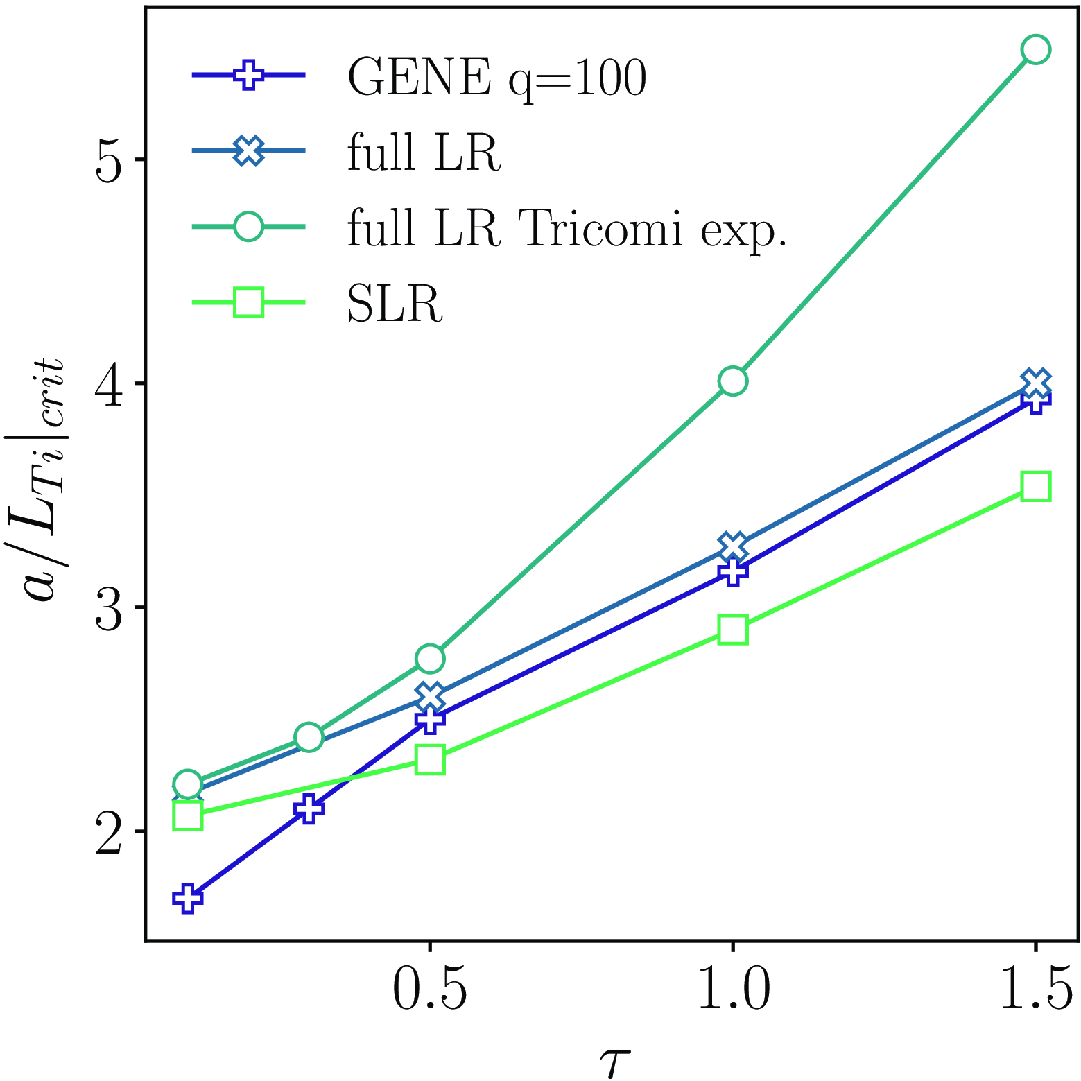
Figure 10. Normalised critical gradient as a function of the temperature ratio $\tau$
calculated for a
$\tau$
calculated for a $q=100$
circular tokamak with the gyrokinetic code GENE compared with the analytical theories with full LR effects and the SLR limit. The Tricomi series expansion of the full LR dispersion relation is also reported. The GENE data is taken from Zocco et al. Reference Zocco, Xanthopoulos, Doerk, Connor and Helander(2018).
$q=100$
circular tokamak with the gyrokinetic code GENE compared with the analytical theories with full LR effects and the SLR limit. The Tricomi series expansion of the full LR dispersion relation is also reported. The GENE data is taken from Zocco et al. Reference Zocco, Xanthopoulos, Doerk, Connor and Helander(2018).
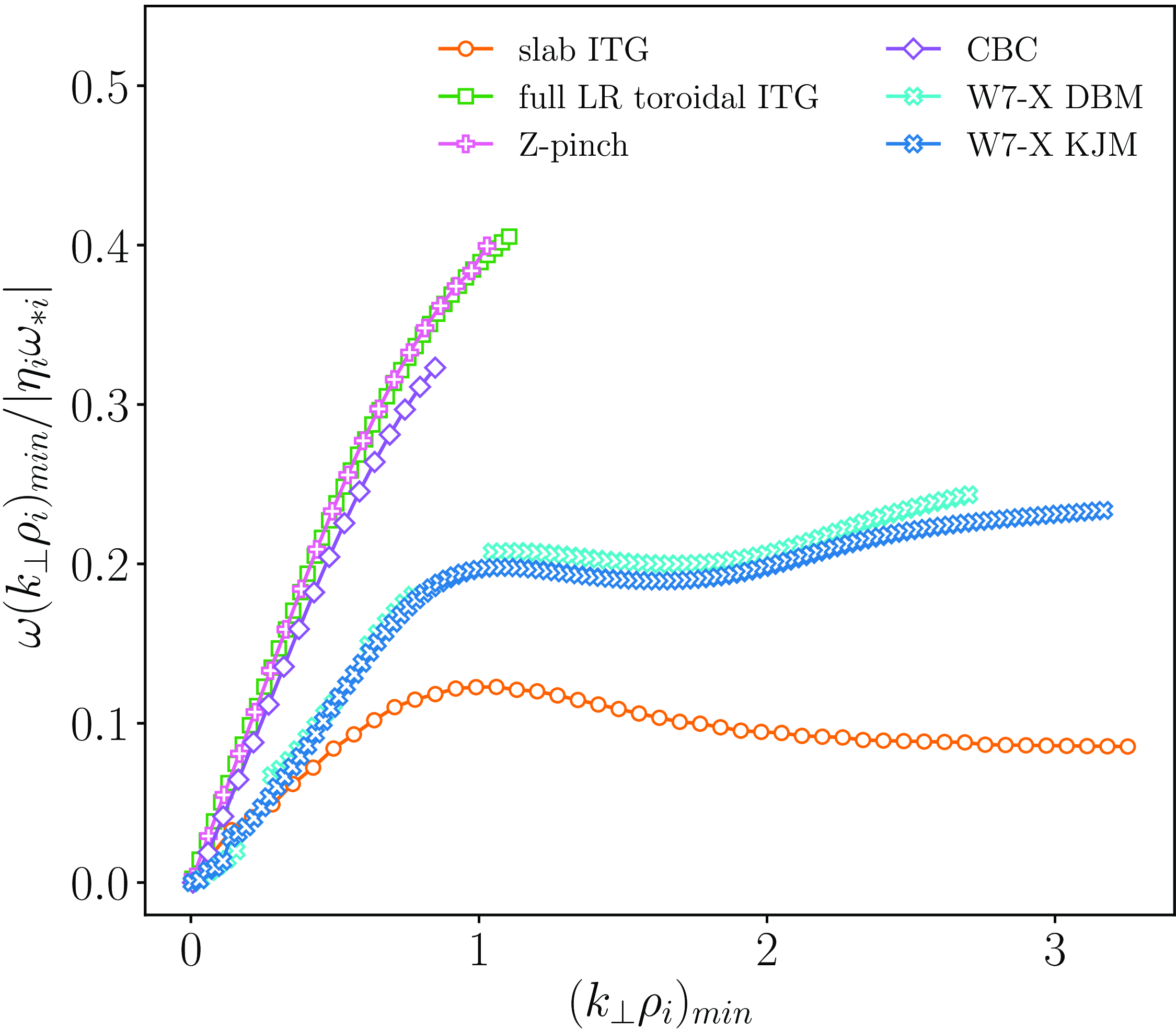
Figure 11. Normalised real frequencies associated with the growth rates shown in figure 1 for an electrostatic and collisionless hydrogen plasma with $\tau =1$
,
$\tau =1$
, $\nabla T_i\neq 0$
and adiabatic electrons.
$\nabla T_i\neq 0$
and adiabatic electrons.
The results are presented in figure 10. We now observe that (3.6) yields, for the critical temperature gradient, quantitative agreement with the GENE code results. The small Larmor radius theory underestimates the critical gradient, particularly at higher $\tau$
values. The plot also includes the Tricomi expansion of the full LR dispersion relation, which we proved to work for small
$\tau$
values. The plot also includes the Tricomi expansion of the full LR dispersion relation, which we proved to work for small $\tau$
values. Although this expansion is not detailed here, it can be found in Appendix D of Zocco et al. Reference Zocco, Xanthopoulos, Doerk, Connor and Helander(2018).
$\tau$
values. Although this expansion is not detailed here, it can be found in Appendix D of Zocco et al. Reference Zocco, Xanthopoulos, Doerk, Connor and Helander(2018).
Appendix B. Real frequencies

Figure 12. Normalised real frequencies associated with the growth rates shown in figure 2 for an electrostatic and collisionless hydrogen plasma with $\tau =1$
,
$\tau =1$
, $\nabla T_i\neq 0$
and kinetic electrons. The W7-X simulation is obtained for
$\nabla T_i\neq 0$
and kinetic electrons. The W7-X simulation is obtained for $a/L_{Ti}=3$
.
$a/L_{Ti}=3$
.
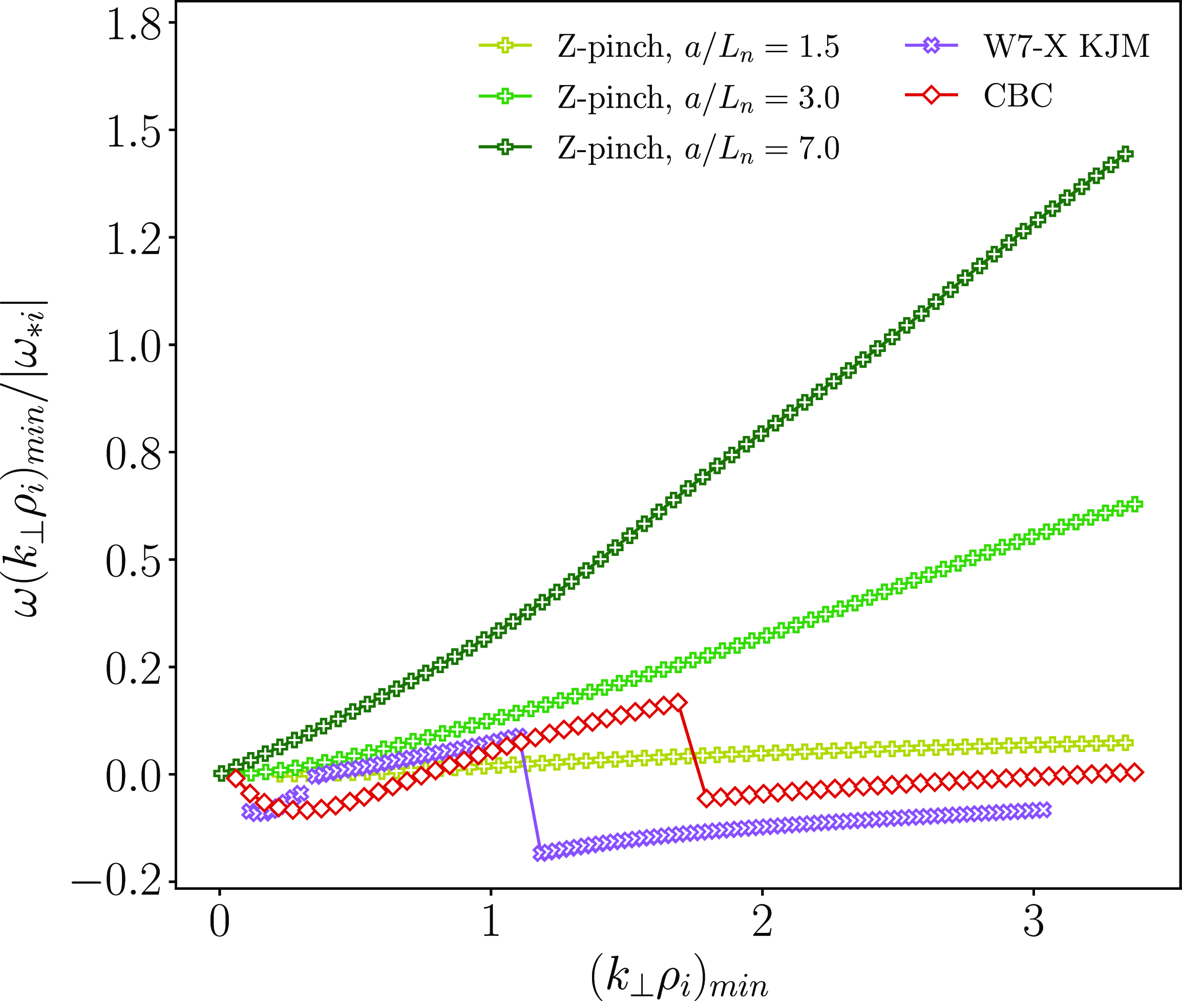
Figure 13. Normalised real frequencies associated with the growth rates shown in figure 3 for an electrostatic and collisionless hydrogen plasma with $\tau =1$
,
$\tau =1$
, $\nabla n\neq 0$
and kinetic electrons. The W7-X and CBC simulations are obtained for
$\nabla n\neq 0$
and kinetic electrons. The W7-X and CBC simulations are obtained for $a/L_n=3$
.
$a/L_n=3$
.
In figures 11–13, we report the normalised normal-mode real frequencies associated with the growth rates used to perform the upper bound theory validation. The real frequencies trends and signs are useful to characterise the nature of normal modes.


 Open access