COUNTEREXAMPLES IN EFFECTIVE TOPOLOGY

Abstract

We prove that there exists a left-c.e. Polish space not homeomorphic to any right-c.e. space. Combined with some other recent works (to be cited), this finishes the task of comparing all classical notions of effective presentability of Polish spaces that frequently occur in the literature up to homeomorphism.

We employ our techniques to provide a new, relatively straightforward construction of a computable Polish space K not homeomorphic to any computably compact space. We also show that the Banach space $C(K;\mathbb {R})$ has a computable Banach copy; this gives a negative answer to a question raised by McNicholl.

We also give an example of a space that has both a left-c.e. and a right-c.e. presentation, yet it is not homeomorphic to any computable Polish space. In addition, we provide an example of a $\Delta ^0_2$ Polish space that lacks both a left-c.e. and a right-c.e. copy, up to homeomorphism.

1. Introduction

The present article contributes to the program in effective topology initiated in the recent independent works [16], [18], and [20]. This program aims to establish the foundations of effective topology, following a similar pattern seen in computable structure theory [12, 15] and computable real analysis [1, 48]. In computable structure theory, most of the results comparing different notions of presentability date back several decades and are generally regarded as classical or foundational. For example, Feiner [13] showed that there is a c.e. presented Boolean algebra without a computable presentation. As an application, Feiner demonstrated that the lattices of X-c.e. and $X'$ -c.e. sets are not isomorphic, for any X. Khisamiev [24] showed that every c.e. presented torsion-free abelian group has a computable presentation, which easily implies a solution to a question about the integral cohomology of finitely presented groups posed in [2]. We see that comparing different notions of algorithmic presentability lead to significant insights in computable algebra, and beyond. In computable analysis, over 70 years ago Specker [45] showed that the notions of Markov (Type 1) and Kleene (Type 2) computability are non-equivalent. Many other definitions that appear throughout the vast literature had been shown to be equivalent to one of these two notions; e.g., [17, 28–30]. Similarly to the situation in computable algebra, Markov and Kleene computability, along with the techniques accumulated in the process of their detailed investigation, form a solid foundation of computable analysis; see the books [1, 40, 48].

In computable topology, there are at least six definitions of an effectively presented Polish space; they will be given in Figure 1 below. These classical notions have been around for a long time; see, e.g., Ceǐtin [7], Moschovakis [37], Spreen [46], Nogina [38], and Kalantari [22]. The problem of comparing these notions strikes us as fundamental. Nonetheless, not all notions that frequently appear in the literature have yet been compared.

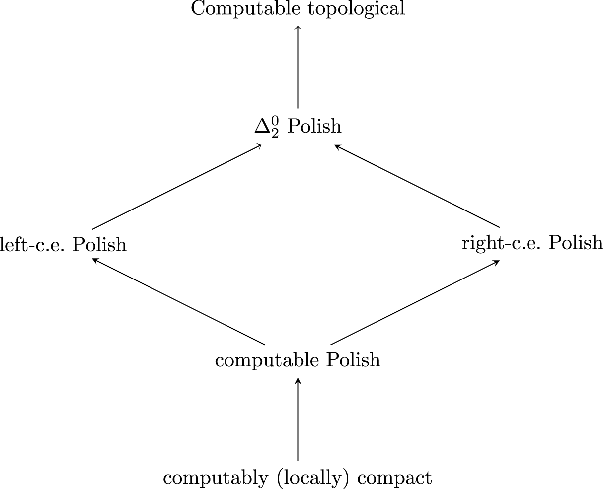
Figure 1 The diagram illustrates the most common notions of computable presentability of (compact) Polish spaces in computable topology. Arrows illustrate the implications between these notions up to homeomorphism. The implication between $\Delta ^0_2$ Polish and computable topological is a recent result established in [4] while the rest of the implications are trivial.

The primary aim of this article is to address this gap. Combined with the cited above papers and some further recent results, our results finish the task of comparing all these notions up to homeomorphism. Before we give the definitions and describe our results, we note that our techniques have already found applications beyond separating the notions in Figure 1. Using our techniques we answer a question of McNicholl by showing that Banach–Stone duality fails effectively. We now turn to the more detailed description of the actual results.

1.1. The main definitions

To state the results formally we need a few well-known definitions. All our spaces are Polish, and we view our spaces up to homeomorphism.

Definition 1 (Essentially Ceitin [8] and Moschovakis [37])

A Polish presentation of a (Polish) space M is given by a countable metric space $X = ((x_i)_{i \in \omega }, d)$ so that the completion of X is homeomorphic to M. A presentation X is:

1. - right-c.e. if $\{r \in \mathbb {Q} : d(x_i, x_j) < r\}$ are c.e. uniformly in $i,j$ ;

2. - left-c.e. if $\{r \in \mathbb {Q} : d(x_i, x_j)> r\}$ are c.e. uniformly in $i,j$ ;

3. - computable if it is both left-c.e. and right-c.e.

The points $x_i$ are usually called special, rational, or ideal.

Both left- and right-c.e. Polish spaces form natural subclasses of $\Delta ^0_2$ Polish spaces. It has been shown in [4] that every $\Delta ^0_2$ Polish spaces admits a computably topological presentation, which is another classical notion of presentability in effective topology. We will not need the notion of a computable topological space, we only note that the implication established in [4] cannot be reversed in general [34]. We will however need the exceptionally robust notion of computable compactness. It admits over a dozen equivalent formulations [11, 21]; one of the many equivalent definitions is as follows.

Definition 2 (Mori, Tsuji, and Yasugi [36])

A (compact) computable Polish space is said to be computably compact if for every n we can produce a finite tuple of special points so that the open $2^{-n}$ -balls centred in these points cover the entire space.

The definition admits a natural generalisation to locally compact spaces which we omit; see [27, 35, 39, 49, 50].

The notions and the implications (up to homeomorphism) between them are summarised in Figure 1 below.

1.2. Completing the diagram

As is carefully explained in [34], all the notions on the diagram with only one exception have been separated in [3, 16, 18, 18, 31]. It was left open in [34, Section 4.1] whether “left-c.e. Polish” implies “right-c.e. Polish” up to homeomorphism. Indeed, it was not known whether “ $\Delta ^0_2$ Polish” implies “right-c.e. Polish”, but evidently a left-c.e counterexample would separate these notions as well. One of the principal aims of the present article it to give such an example. We prove:

Theorem 1.1. There is a locally compact left-c.e. Polish space which is not homeomorphic to any right-c.e. Polish space.

Together with the cited above results, it follows from the theorem that the only implications between these notions are those shown in Figure 1. The result also implies an earlier result [18, 20] that says that there exists a $\Delta ^0_2$ Polish space not homeomorphic to any computable Polish space. Our proof of the stronger Theorem 1.1 is significantly less combinatorially involved than the arguments in [18, 20]. Our proof uses the technique of limitwise monotonic sets to separate the recursion-theoretic combinatorics from definability. The notion of a limitwise monotonic set was first suggested by Khisamiev [19] to characterise computable presentability of (discrete, countable) abelian p-groups. It was later rediscovered by Khoussainov, Nies, and Shore in [25] in the context of computable model theory, and then much more recently (and independently) it was rediscovered again by Bosserhoff and Hertling [5]. For many applications of limitwise monotonicity in effective algebra and computable model theory, see [10, 23].

1.3. A bad closed subset of the unit square

Separating the notion of computable compactness from the notion of a computable Polish space appears to be a non-trivial task. Obviously, one naturally seeks a compact counterexample. There are two proofs in the literature; see [31] and [11] (the latter based on an idea from [20]). Both proofs use a new way of calculating Čech cohomology of a compact space, and the former also used a computable version of Pontryagin Duality. It was raised in [11] whether there is a more elementary ‘direct’ way to construct such an example that, for instance, would not rely on the heavy machinery of algebraic topology or topological group theory. We further extend our definability techniques established in the proof of Theorem 1.1 to prove:

Theorem 1.2. There exists a computably enumerable closed subset K of the unit square $[0,1]^2$ that is not homeomorphic to any computably compact space.

A closed set is computably enumerable (c.e.) if it contains a c.e. sequence of computable points that is dense in the set. Clearly, $K \subseteq [0,1]^2$ from the theorem above can be viewed as a computable Polish space; just use the dense set as the set of special points in K. Our proof of Theorem 1.2 utilises variety of techniques, including a subtle definability lemma extending a result from [18], a new characterisation of computable compactness extending another technical result from [11], and a lemma about limitwise monotonic sets established in [25]. However, our proof is certainly much more straightforward than all previously known proofs, our space is topologically very tame, and the proof is also quite easy to ‘massage’. For instance, it is not hard to use K from Theorem 1.2 to illustrate that Banach–Stone Duality is not effective in general; we discuss this next.

1.4. Banach–Stone Duality is not effective

Recall that one way to state Banach–Stone Duality is as follows. For compact $K_0, K_1$ , the Banach spaces $C(K_0; \mathbb {R})$ and $C(K_1; \mathbb {R})$ are linearly isometric if, and only if, $K_0$ and $K_1$ are homeomorphic. It is clear that when K is computably compact, $C(K; \mathbb {R})$ admits a computable Banach presentation. The latter is a computable Polish presentation of the associated metric space $d(x,y)= ||x -y||$ in which the point $0$ and the operation $+$ are computable. In fact, computability of $0$ follows easily from computability of $+$ . (An equivalent formulation can be found in the book [40].) A few years ago McNicholl asked whether the converse is also true, i.e., whether computable presentability of the Banach space $C(K; \mathbb {R})$ implies that K is homeomorphic to a computably compact space. In [3] it has been shown that if K is a Stone space, then the answer to McNicholl’s question is positive. In other words, Banach–Stone Duality holds computably for Stone spaces. The general case was left open. We prove:

Theorem 1.3. There exists a computable Banach space linearly isometric to $C(K; \mathbb {R})$ where the compact domain K is not homeomorphic to any computably compact Polish space.

This result is perhaps unexpected since it contrasts greatly with the case of Stone spaces discussed above, and with the recently announced effective Gelfand duality between compact K and the respective computable $C^*$ -algebras $C(K;\mathbb {C})$ [6]. However, modulo Theorem 1.2, the proof of Theorem 1.3 is actually not difficult at all. It essentially suffices to take the space K from the proof of Theorem 1.2 and observe that we can easily construct a computable Banach presentation of $C(K; \mathbb {R})$ . (For a further discussion, see Remarks 1 and 2.)

1.5. Two counterexamples

To finish the paper, we give two more applications of our techniques. The results that we present next are mainly motivated by the search for a general enough recursion-theoretic sufficient condition for a space to be computably presented. In computable structure theory, it is sometimes possible to show that if a structure in some natural broad class has a presentation ‘close to being computable’, then the structure has a computable presentation; e.g., [24, 26, 32]. In contrast, Wehner [47] and Slaman [43] built examples of structures having X-computable presentations for any non-computable X, but having no computable presentation. Also, Chisholm and Moses [9] constructed a linear order that is n-decidable for all $n \in \omega $ , but has no decidable isomorphic copy. Further results of this sort can be found in the survey [14]. A similar program in topology has been proposed by Selivanov in [42]. There are still very few results of this sort that can be found in the literature. For example, every left-c.e. Stone space admits a computably compact copy [18, 34]. There exists a compact Polish space that has a X-computable Polish presentation for any $\mathbf {non}$ - $\mathbf {low_2}$ set X, but has no $\mathbf {low_2}$ Polish copy [33]. A few more results can be found in [11, 20]. We establish the following, in our opinion rather surprising, result that fits well into this framework.

Theorem 1.4. There exists a locally compact Polish space M such that M is both right-c.e. presentable and left-c.e. presentable, however M is not homeomorphic to any computable Polish space.

The theorem simultaneously implies several earlier theorems established in [34], [3], and [18]. As we explain in Remark 2, the locally compact space M from Theorem 1.4 can be used to show that the extension of the effecive Banach–Stone theorem to locally compact spaces fails “even more”: this time our locally compact space is not even computable Polish, let alone locally computably compact.

Finally, utilising the definability framework established in the paper, we prove another result that, in a way, complements the theorem above.

Theorem 1.5. There exists a $\Delta ^0_2$ compact Polish space M that is neither homeomorphic to any left-c.e. Polish space nor to any right-c.e. Polish space.

This theorem too implies the main result in [18] and, compared to the argument in [18], its proof is much less combinatorially involved. Limitwise monotonic functions once again play a crucial role in sorting out the combinatorics. We leave open whether examples of this sort exist inside the unit interval (cf. Question 1).

The remainder of the paper is dedicated to proving our results. To avoid the need for a technical preliminaries section, we have chosen to provide the necessary auxiliary technical definitions and results as needed throughout the paper. We however expect that the reader has some background in recursion theory [41, 44] and is familiar with the terminology of (elementary, point-set) topology and metric space theory. The titles of the sections and subsections should be self-descriptive enough to facilitate easy navigation through the paper.

2. A left-c.e. space with no right-c.e. copy

In this section we prove Theorem 1.1.

2.1. Star-spaces and $\epsilon $ -paths

The definability technique based on ‘n-stars’ was invented in [18].

Definition 3. A k-star is a topological space homeomorphic to k copies of the interval $[0,1]$ all joined at one end in a single point (the Wedge sum of k copies of $[0,1]$ via $0$ ). A $0$ -star is an isolated point.

Note that $1$ -star and $2$ -star are homeomorphic, but otherwise a k-star is not homeomorphic to a $k'$ -star when $k \neq k'$ . In what follows next, we always assume that $k \neq 1$ since we identify $1$ -stars and $2$ -stars. We say that a space (a closed set) is a star if it is a k-star.

Definition 4. A nice space is a Polish space in which every path-component is either a singleton, or clopen and is homeomorphic to a star.

We will essentially need only two kinds of nice spaces: a disjoint union of stars and the one-point compactifications of such spaces. We now verify that, in a nice space, we can express the existence of a path between points by saying that for every $\epsilon>0$ , there is an “ $\epsilon $ -path” between these points (to be clarified). Thus, we can arithmetically express that a nice space contains a k-star. The lemma below clarifies this intuition. (But of course, the main challenge is to make the complexity of this statement optimal.)

Let $(M,d)$ be a Polish space. Given special points $x,y$ , an $\epsilon $ -path from x to y is a sequence of points $x = u_0,u_1,\ldots ,u_n = y$ such that $d(u_i,u_{i+1}) < \epsilon $ . An $\epsilon $ -chain between points x and y in a Polish space is a sequence of open balls $B_0, B_1, \ldots , B_k$ having radii $<\epsilon $ such that:

1. (1) $B_i \cap B_{i+1} \neq \emptyset $ , for all $i \leq k$ ;

2. (2) $x \in B_0$ and $y \in B_k$ .

Lemma 2.1. Let $(M,d)$ be a Polish space such that each path-component of M is compact and open. The following are equivalent for points $r,s \in M$ :

1. (1) there is a path between r and s;

2. (2) there is an $\epsilon $ -path between $r,s$ , for any $\epsilon>0$ ;

3. (3) there is an $\epsilon $ -chain between $r,s$ , for any $\epsilon>0$ .

(The implications $(1) \rightarrow (2) \leftrightarrow (3) $ hold without any extra assumptions about the Polish space M.)

Proof. It is easy to see that an $\epsilon $ -path can be viewed as an $2\epsilon $ -chain, and conversely the centres of the balls forming an $\epsilon $ -chain give rise to a $2\epsilon $ -path. This gives the equivalence of $(2)$ and $(3)$ .

Assume $(1)$ , so there is a path between r and s. Let $f \colon [0,1] \to M$ be a continuous path from r to s. Then f is uniformly continuous. For a sufficiently large rational q, we have that for each i, $ d(f\left (\frac {i}{q}\right ),f\left (\frac {i+1}{q}\right )) < \frac {\epsilon }{4}.$ Choose $x_0 = r$ , $x_q = s$ , and for each $i = 1,\ldots ,q-1$ , choose a special point $x_i$ with $d(x_i,f(i/q)) < \epsilon / 4$ . Then $r = x_0,\ldots ,x_q = s$ is an $\epsilon $ -path from r to s.

We now assume $(1)$ fails, and we show there is an $\epsilon>0$ such that there is no $\epsilon $ -path between r and s. Let C be the path-component of r. Since C is open, its complement is closed, and since C is compact, the distance between C and $C^c$ is $\epsilon>0$ . Then there is no $\epsilon /2$ -path from r to s, as given any path $r = u_0,u_1,\ldots ,u_n = s$ there must be a first i such that $u_i \in C$ and $u_i \notin C$ , and so $d(u_i,u_{i+1}) \geq \epsilon $ .

The elementary lemma above will sometimes be used without explicit reference. Note also that every nice space satisfies the premises of the lemma.

2.2. The definability lemma for right-c.e. spaces

Our next definability lemma is a generalisation of the main definability result from [18]. The lemma will be central to the proof of Theorem 1.1.

Lemma 2.2. Let $\left ((\alpha _{i})_{i\in \omega },d\right )$ be a right-c.e. Polish presentation of a nice space $\mathcal {M}$ . Then

$$ \begin{align*} \textit{"a special point }\alpha\in\mathcal{M} \textit{is part of a }(\geq n)\textit{-star"} \end{align*} $$

can be expressed as a $\Sigma ^0_3$ predicate (in $\alpha $ and n).

Proof. The idea is as follows. If we have points $p_0, p_1, p_2$ at separate ‘arms’ of the star, then there is a $\delta>0$ for every sufficiently small $\epsilon $ there must be an $\epsilon $ -path between $p_0$ and $p_1$ which is at distance at least $\delta $ from $p_2$ , and the same is true for any permutation of these three points. The generalisation of this idea to $n>2$ can be used to describe the property claimed in the lemma; this is verified in [18]. However, the issue is that in a right-c.e. space stating this property directly, as in [18], would give a mere $\Sigma ^0_4$ upper bound for the complexity. To circumvent this difficulty, we use compactness. In the notation above, there has to be a fixed $\delta $ -path $x_1,\ldots , x_m$ between $p_0$ and $p_1$ which is $2\delta $ -far from $p_2$ and so that, for any sufficiently small $\epsilon $ , there is an $\epsilon $ -path (essentially) inside this fixed $\delta $ -path. This way we rearrange the quantifiers so that, in a right-c.e. space, we get the complexity for the predicate down to $\Sigma ^0_3$ .

We prove that a special point $\alpha \in \mathcal {M}$ is part of a $(\geq n)$ -star iff the following statement holds:

$\exists p_{1},\dots ,p_{n}$ special points and a rational $\delta>0$ such that

1. $\forall i,j,k \leq n \, \,\exists x_{1},x_{2},\dots ,x_{m}$ special with the properties

   1. (a) $d(p_{k},x_{s})>2\delta $ for every $s \leq m$ ;

   2. (b) $\forall \varepsilon <\delta $ , $\exists \varepsilon $ -path $p_{i}=u_{1},u_{2},\dots ,u_{l}=p_{j}$ such that $\forall r \leq l \, \exists s \leq m \,d(u_{r},x_{s}) <\delta $ .

Let S be a $(\geq n)$ -star. Let $P_{1},P_{2},\dots ,P_{n}$ be distinct arms of S. For each $1\leq i\leq n$ pick $p_{i}\in P_{i}$ at some distance from the ‘centre’ of the star. We can assume therefore that $p_i \in P_{i}^\circ $ which is the interior of $P_i$ homeomorphic to $(0,1)$ . Also pick $\delta =\frac {1}{4}\min \left \{d\left (p_{i},S\setminus P_{i}^{\circ }\right )\mid 1\leq i\leq n\right \}\cup \{\Delta \}$ , where $\Delta $ is the isolating distance of S (i.e., the distance from S to $\mathcal {M} \setminus S$ ). Fix $i,j,k \leq n$ . Since $P_{i}\cup P_{j}$ is compact, there is a finite $\delta $ -cover of $P_{i}\cup P_{j}$ by balls centred in some special $x_{1},x_{2},\dots ,x_{m}$ . Observe also that by choice of $\delta $ , $d(x_{s},p_{k})>2\delta $ for any $1\leq s\leq m$ as $x_{s}\in S\setminus P_{k}^{\circ }$ . Recall Lemma 2.1. Since $p_{i},p_{j}$ are connected in $P_{i}\cup P_{j}$ , for any $\varepsilon <\delta $ there is an $\varepsilon $ -path $p_{i}=u_{1},u_{2},\dots ,u_{l}=p_{j}$ where each $u_{r}\in P_{i}\cup P_{j}$ . It follows that $\forall r \,\exists s\,d(u_{r},x_{s})<\delta $ .

Now assume the property holds. It follows from Lemma 2.1 that the points $p_1 \ldots p_k$ lie in the same path component. Thus, the path-connected component S has to be a star. Suppose then that S is not a $(\geq n)$ -star, that is S has $<n$ arms. Then by the pigeonhole principle, for any choice of $p_{1},p_{2},\dots ,p_{n}$ , there are at least two of the chosen points which lie on the same arm, say $p_{1},p_{3}\in P_{1}$ . Let $\delta>0$ be given, and we pick from $p_{1},\dots ,p_{n}$ the points $p_{1},p_{2}$ and $p_{3}$ . If $p_{2}\in P_{1}$ , then we can induce an ordering on $p_{1},p_{2},p_{3}$ by considering their preimage in $[0,1]$ , as $P_{1}$ is the homeomorphic image of $[0,1]$ . Then one of the special points must be between the other two with respect to this ordering. Let this point be $p_{k}$ . (In the case when $p_{2}\notin P_{1}$ , then let either $p_{1}$ or $p_{3}$ be $p_{k}$ depending on which has the preimage closer to $0$ in $[0,1]$ .) Without loss of generality, we assume that $p_{3}$ is chosen to be $p_{k}$ .

Now let $x_{1},x_{2},\dots ,x_{m}$ be given such that $d(p_{2},x_{s})>2\delta $ for each s. If $p_{1}\in B_{\delta }(p_{3})$ or $p_{2}\in B_{\delta }(p_{3})$ , then fix any $\varepsilon $ -path $p_{1}=u_{1},u_{2},\dots ,u_{l}=p_{2}$ , where $\varepsilon <\delta $ . It cannot be that $\forall r \,\exists s \,d(u_{r},x_{s})<\delta $ . In the case when $p_{1}\in B_{\delta }(p_{3})$ , we have $d(p_{3},x_{s})<2\delta $ , and in the case when $p_{2}\in B_{\delta }(p_{3})$ , we have that $d(u_{l},x_{s})<2\delta $ for some s. Thus we can assume that $S=B_{\delta }(p_{3})\sqcup F_{1}\sqcup F_{2}$ where $F_{1},F_{2}$ are disjoint compact sets of $S \setminus B_{\delta }(p_{3})$ containing $p_{1}$ and $p_{2}$ , respectively. Then pick $\varepsilon =\frac {1}{4}\min \{\delta ,d\left (F_{1},F_{2}\right ),\Delta \}$ , and fix an $\varepsilon $ -path $p_{1}=u_{1},\dots ,u_{l}=p_{2}$ . Since $F_{1}\cap F_{2}=\emptyset $ , there must be some first index r for which $u_{r}\notin F_{1}$ . By the choice of $\varepsilon $ , it follows that $u_{r}\in B_{\delta }(p_{3})$ , which is to say that $\exists s,\,d(u_{r},x_{s})<\delta $ , a contradiction.

2.3. Proof of Theorem 1.1

Fix $\Sigma ^0_3$ sets $R,S \subseteq \omega $ and the standard computable pairing function $\langle \cdot , \cdot \rangle $ . We will define a locally compact space

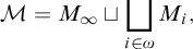$$ \begin{align*}\mathcal{M}= M_\infty \sqcup \bigsqcup_{i \in\omega}M_{i},\end{align*} $$

where $M_n, M_\infty $ are clopen components in M with the following properties:

1. i $M_\infty $ is a countable discrete subspace with all points at distance $\geq 10$ from each other.

2. ii For each $i\in \omega ,\,M_{i}\subseteq [0,1]^{2}$ under the standard Euclidean metric on $[0,1]^{2}$ .

3. iii For $\alpha ,\beta $ from different clopen components $M_i$ ( $i \in \omega $ ), $d(\alpha ,\beta )=2$ . The distance from any point in $M_i$ to any point in $M_\infty $ is $\geq 10$ .

We now describe the clopen components $M_{i}$ in a bit more detail. For that, fix the standard computable pairing function $\langle \cdot , \cdot \rangle $ .

1. iv If $n\notin R$ , then $M_{\langle n, j \rangle }$ is finite for every j.

2. v If $n\in R$ and $n\notin S$ , then there is a unique j such that $M_{\langle n, j \rangle }$ is a $(n+3)$ -star, and when $j \neq j'$ the component $M_{\langle n, j' \rangle }$ is finite.

3. vi If $n\in R$ and $n\in S$ , then there is a unique j such that $M_{\langle n, j \rangle }$ is a disjoint union of $(n+3)$ line segments, and when $j \neq j'$ the component $M_{\langle n, j' \rangle }$ is finite.

In iv–vi, the exact cardinality of finite components will depend on the effective approximation of the $\Sigma ^0_3$ sets. In fact, these cardinalities are not important to us since they will not effect the properties of the space that we need to prove the theorem. The exact definition of the distance in i and $iii$ is also not important and will depend on S and R as well.

Lemma 2.3. There is a uniform procedure that, given (indices of) $\Sigma ^0_3$ sets $R, S$ outputs a locally compact left-c.e. Polish space $\mathcal {M} = \mathcal {M}_{R,S}$ satisfying the properties i–vi.

Proof. We represent $R(n)$ as $\exists j \exists ^{\infty } m U (j,m,n)$ and $S(n)$ as $\exists j \exists ^{\infty } m V (j,m,n)$ , where $U,V$ are computable predicates. We can further assume that the predicate U satisfies the unique witness property, i.e., if $\exists j \exists ^{\infty } m U (j,m,n)$ then there is a unique j. For V, we assume that if $\exists ^{\infty }m V(j,m,n)$ , then for all $j'>j$ , we also have $\exists ^{\infty } m U(j',m,n)$ .

For every j, we build the component $M_{\langle n, j \rangle }$ as follows. We monitor $U (j,m,n)$ and act in the $M_{\langle n, j \rangle }$ -component only when a fresh witness m is discovered for n. In particular, if there are only finitely many such m for the fixed n and j, then $M_{\langle n, j \rangle }$ will remain finite.

Assuming $U (j,m,n)$ keeps providing us with m-witnesses, we proceed to build $M_{\langle n, j \rangle } \subseteq [0,1]^{2}$ as follows. We put more points into $n+3$ arms of (some fixed ahead of time) presentation of a $(n+2)$ -star inside $ [0,1]^{2}$ . The procedure with which points are put into the arms of the star is additionally controlled by the predicate V. We subdivide each arm into sub-intervals $(2^{-j'-1}, 2^{-j'}]$ and monitor V. Every time we discover a new V-witness m for $j'$ , we move all points that we put so far into $(2^{-j'-1}, 2^{-j'}]$ to the component $M_\infty $ making the distances between these points (and the distances from these points to the rest of the points present so far in the space) larger than any number seen so far in the construction.

It is evident that the resulting space is locally compact, left-c.e., and satisfies i–vi.

A set of natural numbers X is limitiwise monotonic if

$$ \begin{align*}X = \text{ range } \sup_y g(x, y),\end{align*} $$

where $\sup _{y}g(x,y)<\infty $ for each x, and g is a computable function.

Lemma 2.4. Suppose $\mathcal {M}_{R,S}$ constructed in the previous lemma has a right-c.e. presentation. Then the set

$$ \begin{align*}X = \{ n : \mathcal{M}_{R,S} \text{ has a }(n+3)\text{-star component} \}\end{align*} $$

is limitiwise monotonic relative to $0"$ .

Proof. First, note that the space is nice (Definition 4). Fix a right-c.e. presentation of $\mathcal {M}_{R,S}$ . Apply Lemma 2.2 to build a $0"$ -computable g with $X = \text { range } \sup _s g(y, s)$ as follows. For a fixed special point $p_y$ , initially keep $g(y,s)$ undefined. Apply Lemma 2.2 to $0"$ -effectively guess whether y is in an l-star component for some $l \geq n \geq 3$ . If we see such an n at stage t, we define $g(y,t) = n-3$ and proceed to the next stage.

To finish the proof of the theorem, we need the following.

Lemma 2.5 (Khisamiev)

There is a d-c.e. set (i.e., a difference of two c.e. sets) that is not limitwise monotonic.

A relatively modern proof of this fact can be found in [25] where a d-c.e. set X with this property is constructed. Relativise this result to $0"$ and fix $\Sigma ^0_3$ sets $R, S$ such that $X = R \setminus S$ . Let $\mathcal {M}_{R,S}$ be the left-c.e. space built in Lemma 2.3. By Lemma 2.4 the space has no right-c.e. presentation.

3. A bad c.e. subset of $[0,1]^2$

In this section we give a detailed proof of Theorem 1.2. We assume that the reader is familiar with the classical concept of Alexandroff’s 1-point compactification of a space.

Definition 5. A star-space is the 1-point compactification of the disjoint union of stars.

In a star-space, the connected components are exactly the path-components, they are clopen, and also they are exactly the n-stars that occur in M. In particular, every star-space is ‘nice’ (Definition 4).

Definition 6. Let M be a compact space. A system of open $2^{-k}$ -covers of the space is a sequence $(C_k)_{k \in \omega }$ of finite sets $C_k$ of open balls in M such that

1. (1) $C_k$ is a cover of M, and

2. (2) every ball in $C_k$ has radius at most $2^{-k}$ .

Our next lemma is a modification of a lemma established in [18].

Lemma 3.1. Suppose that M is a star-space, and let $(C_k)_{k \in \omega }$ be a system of finite open $2^{-k}$ -covers of the space. A special point r is contained within an s-star with $s \geq \ell>1$ if and only if

1. (*) there exist $ B(p_1, \gamma _1), \ldots , B(p_\ell , \gamma _\ell ) \in \bigcup _k C_k $ and $m \in \mathbb {N}$ , and with the properties:

2. $p_0, \ldots , p_\ell $ lie in the same connected component as r and

3. $\forall n>m$ and any $i,j,k<\ell $ , there is a $2^{-n}$ -chain $\subseteq C_n$ from $p_i$ to $p_j$ avoiding $B(p_k,\gamma _k)$ .

Proof. If r is the point of infinity used in the definition of the 1-point compactification, then we cannot possibly find $p_1,p_2,\ldots ,p_\ell $ in the path-component as r (recall $\ell>1$ ). Thus, we may assume r comes from one of the star-components.

We show that ( $*$ ) holds when r lies in an n-star S, $n \geq \ell $ . Fix small enough balls $B(p_1, \gamma _1), \ldots , B(p_\ell , \gamma _l) $ in the system of covers which are centred in $p_1,\ldots ,p_\ell $ that belong to different arms of the star S, which is the connected clopen component of r. Given $p_i$ , $p_j$ , and $p_k$ , we can assume their radii $\gamma _k$ are so small that $B(p_k, \gamma _k)$ does not intersect the arms containing $p_i$ and $p_j$ , and also does not intersect the clopen (thus, compact) complement of the star. Then there is a path P between $p_i$ and $p_j$ in $M - B(p_k, \gamma _k)$ .

The path P is compact, thus the distance between P and the closure of $B(p_k, \gamma _k)$ is non-zero; say it is $\theta _k$ . Let $2^{-n}< \theta _k/2$ . The finite set of $2^{-n}$ -balls $C_n$ is a cover of M, and thus of S and of P as well. If we remove all balls in $C_n$ that do not intersect P, then each remaining ball cannot possibly intersect $B(p_k, \gamma _k)$ . The resulting cover U can be further refined to a $2^{-n}$ -chain from $p_i$ to $p_j$ that does not intersect $B(p_k, \gamma _k)$ .

Take any ball in U that contains $p_i$ ; denote it $B_1$ . Consider the compact set $P \setminus B_1$ , and note that $U \setminus \{ B_1 \}$ has to cover this set. At least one ball in $U \setminus \{B_1\} $ has to intersect $B_1$ since P is connected; let this ball be $B_2$ . Continue in this way to define $B_3$ , $B_4$ , $\ldots $ until $P \setminus \cup _{i<t} B_i = \emptyset $ . Since U is finite and is a cover of P, this process must terminate. Let $U_0 \subseteq U$ be the collection of balls constructed by this iterated process. There exists a ball $B_k \in U_0$ so that $p_j \in B_k$ . Consider the graph in which the balls in $U_0$ are the vertices and the edge relation holds between $B_i $ and $B_j$ iff $P \cap B_i \cap B_j \neq \emptyset $ . The graph is connected, and there must be a path between $B_1 \ni p_i$ and $B_k \ni p_j$ . The balls along this path in the graph form an $\epsilon $ -chain.

It remains to fix any $m> max_{ k \leq \ell }(- \log _2 \theta _k/2$ ).

Now let S be an s-star in M with $s < \ell $ . Suppose $ B(p_1, \gamma _1), \ldots , B(p_\ell , \gamma _l) \in \bigcup _n C_n $ having their centers in S. For some $i,j,k$ , after removing $p_k$ , the star splits into two connected components, one containing $p_i$ , and the other containing $p_j$ . We may assume that $\gamma _k$ is sufficiently small that $p_i,p_j \notin B(p_k, \gamma _k)$ ; otherwise there is nothing to prove. It is sufficient to show that for every $\delta $ , there is an $\epsilon < \delta $ such that for every $\epsilon $ -path $p_i = u_0,u_1,\ldots ,u_n = p_j$ from $p_i$ to $p_j$ , there is some $u_i \in B(p_k, \gamma _k)$ . By Lemma 2.1, it will imply that $\epsilon '$ -chains for sufficiently small $\epsilon '$ will also have to intersect $B(p_k, \gamma _k)$ (indeed, we could just take $\epsilon ' = 2\epsilon $ ). In fact, any such $\epsilon '$ -chains will have this property, not just those made up from balls in $\bigcup _n C_n$ .

The star S splits into the disjoint union $C_i \sqcup C_j \sqcup B(p_k, \gamma _k)$ where $C_i$ and $C_j$ are closed sets containing $p_i$ and $p_j$ respectively. Then $C_i$ and $C_j$ are compact, and so we can choose $\epsilon $ smaller than the distance between $C_i$ and $C_j$ , and also smaller than the distance between S and the complement of S. Then any $\epsilon $ -path $p_i = u_0,\ldots ,u_n = p_j$ in M must have $u_0,\ldots ,u_n \in S$ (since the distance between S and the complement of S is greater than $\epsilon $ ). Also, since $u_0 \in C_i$ , $u_n \in C_j$ , and the distance between $C_i$ and $C_j$ is greater than $\epsilon $ , for some s, $u_s \in B_{\delta }(p_k)$ .

3.1. Computably compact star-spaces

We return to the analysis of star-components, but this time in a compact space. Recall that a computable Polish space is computably compact if there is an effective enumeration of (finite tuples coding) all finite covers of the space by basic open balls. Recall that a star-space is the 1-point compactification of the disjoint union of n-stars, for various $n \neq 1$ (perhaps with repetition).

Proposition 3.2. Let M be a computably compact presentation of a star-space. Then the set

$$ \begin{align*}\{n>1: M \text{ has an }n\text{-star component} \}\end{align*} $$

is $0'$ -limitwise monotonic.

Proof. Recall that a basic computable ball is a ball centred in a special points and having a computable radius (as opposed to rational radius represented as a fraction in a basic ball). It has been shown in [11] that every computably compact Polish space admits a uniformly computable system of finite $2^{-n}$ -covers $(C_n)$ , $n =1,2,3 \ldots $ , consisting of computable basic balls with the following properties:

1. (1) each ball in $C_n$ has radius at most $2^{-n}$ ;

2. (2) each $C_n$ is (uniformly) represented by a finite tuple of indices coding these centres and the radii of the balls making up $C_n$ ;

3. (3) for any finite collection of balls $X_0, \ldots , X_k \in \bigcup _n C_n$ (represented by their indices) we can uniformly decide whether

   $$ \begin{align*}X_0 \cap \ldots \cap X_k \neq \emptyset.\end{align*} $$

We follow the terminology in [11] and say that such a system of cover $(C_n)$ is strongly $\cap $ -decidable.

Lemma 3.3. Let M be a computably compact Polish space with special points $(x_i)$ . There is a strongly $\cap $ -decidable system of covers $(C_n)$ for which the relation ‘ $x_i \in X$ ’ is uniformly decidable for any $X \in \bigcup _n C_n $ and $i \in \omega $ .

Proof. We first discuss the informal idea. The key observation is that all conditions that are sufficient to satisfy to prove the lemma are effectively open sets. Note, for example, that every intersection of the form $X_0 \cap \ldots \cap X_k \neq \emptyset $ has to be witnessed by a special point. Thus, (slightly) decreasing the radii will still preserve $X_0 \cap \ldots \cap X_k \neq \emptyset $ . On the other hand, if we had $X_0 \cap \ldots \cap X_k = \emptyset $ , then decreasing the radii will obviously preserve this property as well. Also, ‘being formally included in’ is an open property of the real parameters describing the balls, thus slightly changing the radii will preserve the formal inclusion between members of $C_{n+1}$ into $C_n$ . We will therefore search for small enough $\epsilon $ so that all these properties of $C_n$ are preserved after decreasing the radii of all balls in $C_n$ by $\epsilon $ , and so that the new radii are not equal to one more real in the list $( d(x_i, x_j))_{i,j}$ , to make sure ‘ $x_i \in X$ ’ is uniformly decidable. We proceed in this way diagonalising against each $d(x_i, x_j)$ for each member in $C_n$ , for every n, one at a time.

We now give formal details.

For a basic open B, we write $B^c$ for the basic closed ball with the same centre as B, and we write $\overline {B}$ to denote the closure of B that does not have to be equal to $B^c$ in general.

Claim 3.4. Suppose M is computably compact. Then, for basic closed balls $B_i^c$ and $B_j^c$ , the property $B_i^c \cap B_j^c = \emptyset $ is c.e. uniformly in $i,j$ . The same is true for any finite collection of basic closed balls.

Proof. The open set $M \setminus B_i^c$ is c.e.. Indeed, we just list all the basic open balls that are formally disjoint from $B_i^c$ via the following standard argument. Every point in $M \setminus B_i^c$ has the property $d(cntr(B_i), y)> r(B_i) =r$ , and if we take $B(y, q)$ where

$$ \begin{align*}0< q <\frac{d(cntr(B_i), y)- r(B_i)}{2}\end{align*} $$

then $d(cntr(B_i), y)> r+q.$ Thus, the union of the complements, which is the complement of the intersection $B_i^c \cap B_j^c$ , is also c.e. open. It covers the space if, and only if, the intersection is empty. By computable compactness of M, this is c.e. The case of finitely many balls is similar.

In the lemma below, $K'$ plays the role of $C_n$ and $\delta $ should be thought of as small enough so that when we ‘shrink’ each ball in $K'$ by $\delta $ , it remains a cover; and parameter $\gamma $ will allow us to iterate the claim. We fix a computably compact M.

Claim 3.5. For every $\epsilon>0$ and $\delta>0$ and any finite cover $K'$ consisting of basic open balls, and a finite collection of computable reals $\Xi = \{\xi _0, \ldots , \xi _s \}$ we can effectively find a finite basic open $\epsilon $ -cover K, a rational $\gamma>0$ , and a finite cover $K"$ such that:

1. (i) Every ball in $K"$ has the same centre as some ball in $K'$ but its radius is at most $\delta $ -smaller;

2. (ii) for each basic open $B_1, \ldots , B_k \in K" \cup K$ , either $ \bigcap _{i \leq k} B_i^c = \emptyset $ or $\bigcap _{i\leq k} B_i \neq \emptyset $ holds;

3. (iii) The radii of all balls in $K" \cup K$ do not lie in $\Xi $ ;

4. (iv) The rational $\gamma>0$ is so that the properties $(i) -(iii)$ are invariant under at most $\gamma $ -change of the radii of all balls in $K" \cup K$ .

Proof of Claim 3.5

Fix a finite $\epsilon /2$ -cover of the space by basic open balls, and replace each ball in the cover with a $\epsilon $ -ball with the same centre. Let S be this new $\epsilon $ -cover. Recall that $B^c$ denotes the basic closed ball with the same centre as B.

For each tuple of basic open $B_1, \ldots , B_k \in S \cup K'$ (exactly) one of the possibilities is realised:

1. (a) $ \bigcap _{i \leq k} B_i^c = \emptyset $ , or

2. (b) $\bigcap _{i\leq k} B_i \neq \emptyset $ , or

3. (c) $ \bigcap _{i \leq k} B_i^c \neq \emptyset $ but $\bigcap _{i\leq k} B_i = \emptyset $ .

Note that there are only finitely many conditions in total, and that both $(a)$ and $(b)$ are c.e. conditions (Claim 3.4).

If we shrink the radii of all $B \in S$ by a $\delta '< \min \{ \delta , \epsilon /2 \}$ (but keep the same centres), then the conditions of the form $(a)$ will still hold, and the smaller balls will still cover the space because the $\epsilon /2$ -balls do. If $\delta '$ is small enough, then the conditions of the form $(b)$ will also still be satisfied, since there are only finitely many conditions like that involved. Note that the third alternative must be witnessed only by points y such that, for some $B_i = B(c_i,r)$ , $d(y,c_i) =r$ . This means that, after we shrink the radii by $\epsilon /2>\delta '>0$ , $(b)$ will still hold for each tuple of balls, but we completely exclude the third alternative. Clearly, a rational $\gamma $ claimed in $(iv)$ also exists, since we could further slightly shrink or expand the balls and still have the same properties satisfied for the resulting balls after this variation. We can search for a $\gamma $ so that any parameter within a $\gamma $ -interval of the found ones still do the job; this is done simply by looking at the extremes of the respective $\gamma $ -intervals defining the radii. Since there are only finitely many computable reals in $\Xi $ , its complement is dense open in $\mathbb {R}$ , thus we can effectively avoid $\Xi $ . Define $K"$ to be the balls in $K'$ after the shrinking, and K is the shrunken balls from S.

The rest of the proof proceeds by induction; we iteratively apply Claim 3.5 to produce a system of covers that satisfies the required properties. For that, we fix an effective enumeration $\Xi = \bigcup _s \Xi _s$ of all reals of the form $d(x_i, x_j)$ , where $x_i, x_j$ range over all special points. We begin with any cover at the first iteration of the procedure. In each consequent iteration of the claim, we also additionally choose the parameters $\gamma $ and $\delta $ are so small that all conditions achieved at the previous stages are maintained at the next stage.

To this end, we fix a strongly $\cap $ -decidable system of covers of M with the additional property provided by Lemma 3.3. Note that the non-singleton clopen components in M are exactly the k-stars ( $k>1$ ) that occur in M.

Lemma 3.6. Using $0'$ , we can effectively enumerate all special points in M that are contained in non-singleton clopen components of M.

Proof. Using a computable list of covers, it not difficult to effectively enumerate all clopen components; e.g., [11, Lemma 4.21]. Each such component is represented in this list as a finite union of basic open (or closed) balls. For a tuple of balls representing a component, we can use $0'$ ask whether it splits further. We can also check using $0'$ whether it contains more than one special point; since it is open, this is equivalent to checking whether it is a singleton.

Working effectively in $0'$ , we produce a list of all special points coming from n-stars, $n>1$ . In this list, each special r also comes with the finite open name of its component. When r is one such point from this list, by Lemma 3.1, it is contained in a k-star for some $k\geq \ell>1$ if and only if:

1. (⋆) there exist $ B(p_1, \gamma _1), \ldots , B(p_\ell , \gamma _\ell ) \in \bigcup _k C_k $ and $m \in \mathbb {N}$ , and with the properties:

2. $p_0, \ldots , p_\ell $ lie in the same connected component as r and

3. $\forall n>m$ and any $i,j,k<\ell $ , there is a $2^{-n}$ -chain $\subseteq C_n$ from $p_i$ to $p_j$ avoiding $B(p_k,\gamma _k)$ .

Recall that parameter r comes with a finite union of basic open balls making up the connected clopen component of r. Thus, we can list all special points in this component given r and the finite parameters describing its component. Since $(C_n)$ is strongly $\cap $ -decidable and also satisfies Lemma 3.3, we claim that we can effectively verify whether

$$ \begin{align*}\text{there is a }2^{-n}\text{-chain chosen from the balls in }C_n\text{ from }p_i\text{ to }p_j\text{ avoiding }B(p_k,\gamma_k).\end{align*} $$

Indeed, this property fails if, and only if, after removing all balls from $C_n$ that intersect $B(p_k,\gamma _k)$ , we end up with two disjoint finite sets of balls, one containing $p_i$ and the other $p_j$ . This can be checked effectively, and thus

$$ \begin{align*}r\text{ is contained in a }k\text{-star for some }k\geq \ell>1\end{align*} $$

is a $\Sigma ^0_2$ -relation uniformly in $\ell $ ; denote this relation by $\Theta _{\geq \ell }$ . For future reference, we state it in the form of a claim.

Claim 3.7. In a computably compact star-space, the relation

$$ \begin{align*}r\text{ is contained in a }k\text{-star for some }k\geq \ell>1\end{align*} $$

is $\Sigma ^0_2$ (in r and $\ell $ ), where r is special and $\ell \in \omega $

Finally, given r, define

$$ \begin{align*}g(r) = \sup_{\ell>1} \{\Theta_{\geq \ell}(r) \text{ holds}\}.\end{align*} $$

Using $0'$ , we can effectively approximate g from below; cf. Lemma 2.4. When r ranges over all special points, $g(r)$ ranges over

$$ \begin{align*}\{n>1: M \text{ has an }n\text{-star component} \},\end{align*} $$

witnessing that the latter set is $0'$ -limitwise monotonic.

3.2. Proof of Theorem 1.2, completed

We build a c.e. closed subset $K \subseteq [0,1]^2$ that is not homeomorphic to any computably compact Polish space. Modulo the definability techniques developed in the previous subsection, the proof of this proposition is elementary. (We will need some properties of the simple construction of K to simplify our proof of Theorem 1.3.)

Proof. Relativise Lemma 2.5 to $0'$ and fix a $\Sigma ^0_3$ set X that is not $0'$ -limitwise monotonic. Without loss of generality, assume that $0 \in X$ and $1 \notin X$ . Fix a computable predicate P such that

$$ \begin{align*}n \in X \iff \exists z \exists^{\infty} y P(z,y,n).\end{align*} $$

For each $k = \langle n, z \rangle $ , reserve a square region $S_k$ of diameter $2^{-k}$ in $[0,1]^2$ ; arrange it so that, as k goes to infinity, these regions converge to the point $(0,0)$ . In each such fixed $S_k$ , where $k = \langle n, z \rangle $ , initiate an approximation of (a dense sequence whose closure is homeomorphic to) an n-star. Initially, place a special point representing the ‘center’ of the star, and place n points at the opposite ‘end’ of its ‘arm’.

Every time $P(z,y,n)$ ‘fires’ (i.e., one more witness y is discovered for the fixed $n,z$ ), place one more point inside each arm in such a way that, if P ‘fires’ infinitely often then we end up with $S_k$ homeomorphic to the n-star. Otherwise, we end up with finitely many points inside $S_k$ . Let $X_k$ be the subset of $S_k$ enumerated by this procedure.

The resulting compact set $K = cl(\cup _{k \in \omega } X_k) \subseteq [0,1]^2$ is evidently c.e. closed, and it is homeomorphic to a star-space with the point $(0,0)$ playing the role of the point of infinity.

Further, we evidently have

$$ \begin{align*}X = \{n>1: K \text{ has an }n\text{-star component} \}, \end{align*} $$

which is not $0'$ -limitwise monotonic. By Proposition 3.2, K is not homeomorphic to any computably compact Polish space.

In view of the discussed above results of Bosserhoff and Hertling [5], we would like to know the answer to:

Question 1. Is there a c.e. closed subset of $[0,1]$ not homeomorphic to any computably compact space?

We leave the question open, and we suspect that new ideas and techniques will be necessary to attack this question.

4. Applications

4.1. A ‘bad’ $\Delta ^0_2$ space

In this subsection we apply our techniques and results to prove Theorem 1.5. Recall that the theorem claims that there exists a $\Delta ^0_2$ compact Polish space that is neither homeomorphic to any left-c.e. Polish space nor to any right-c.e. Polish space.

The key lemma is as follows.

Lemma 4.1. Suppose M is a left-c.e. presentation of a compact Polish space. Then M is $0'$ -computably compact.

Proof. As explained in [11] in much detail, it is sufficient to $0'$ -effectively produce at least one $2^{-n}$ -cover for each $n \in \omega $ . Given a finite collection of basic open balls $B_0, \ldots , B_k$ of radius $2^{-n-1}$ represented by their special centres (and $-n-1$ ), check whether there is a special point outside of all these open balls. Since the space is left-c.e., it is a $\Sigma ^0_1$ condition that can be decided using $0'$ . If there is such a special point, then $B_0, \ldots , B_k$ is not a cover. On the other hand, if no such special point exists then the $2^{-n}$ -balls with the same centres as $B_0, \ldots , B_k$ is a cover of the entire space. It is clear that going through all possible finite tuples of basic open $2^{-n-1}$ -balls we will eventually find at least one such tuple that covers all special points.

If M is a left-c.e.-presentable star-space then, by Lemma 4.1 and Claim 3.7 (relativised to $0'$ ), we have that the relation

$$ \begin{align*}r\text{ is contained in a }k\text{-star for some }k\geq \ell>1\end{align*} $$

is $\Sigma ^0_3$ (in r and $\ell $ ), where r is special and $\ell \in \omega $ . Similarly, in a right-c.e. presented star-space this relation is also $\Sigma ^0_3$ , by Lemma 2.2. In both cases we can conclude that the set of all $n>3$ so that the space contains an n-star has to be limitwise monotonic relative to $0"$ .

The rest of the proof is very similar to the proof of Lemma 2.3, with only two elementary modifications. Recall that in Lemma 2.3 we constructed a left-c.e. presentation of a space of the form $\mathcal {M}= M_\infty \sqcup \bigsqcup _{i \in \omega }M_{i}$ . This was done using approximations to $\Sigma ^0_3$ sets $R,S \subseteq \omega $ so that $R \setminus S$ is not $0"$ -limitwise monotonic. We repeat the same proof but this time:

1. (1) We do not have $M_\infty $ .

2. (2) We arrange $M_{i}$ on $[0,1]^2$ (shrinking their diameters) so that they converge to, say, the point $(0,1)$ .

3. (3) In the proof, instead of moving finitely many points to $M_\infty $ we simply erase them from the space. (We may reintroduce these points later again.)

This way we construct a $\Sigma ^0_2$ -closed subspace of $[0,1]^2$ that evidently also gives a $\Delta ^0_2$ -Polish presentation of the space. However, since the sizes of the stars in the space code a set that is not $0"$ limitwise monotonic, the space cannot possibly have a left c.e. presentation nor a right-c.e representation.

4.2. The effective Banach–Stone Duality fails

Let K be the c.e. subset of $[0,1]^2$ constructed in Section 3.2; it has no computably compact copy. It has the form $\{(0,0) \} \cup \bigcup _k X_k$ , where each $X_k$ is either a dense subset of an n-star for (where $k = \langle n, z \rangle $ for some z), or is an ‘incomplete’ n-star, i.e., a finite subset on an n-star that contains the centre, the end-points of its arms, but only finitely many points in-between these points on the arms.

Let $X_{k,s} \subseteq X_k$ be the part of $X_k$ produced at the end of stage s of the construction in Section 3.2. Since each $X_{k,s}$ can be thought of as a subset of a copy of the n-star (which may or may not become a part of K in the limit), it makes sense to talk about generalised piecewise linear functions $f: X_{k,s} \rightarrow \mathbb {R}$ , which are defined as follows. A function is generalised piecewise linear on an n-star if it is linear when restricted to each arm of the star. Then we say that a function is generalised piecewise linear on $X_{k,s}$ if it is the restriction of a generalised piecewise linear function with support the respective n-star $\subseteq [0,1]^2$ reserved for $X_k$ . (We also assume its support does not exceed $X_k$ .)

We add special points in $C(K; \mathbb {R})$ to represent the following functions:

1. (1) All piecewise linear functions on $X_{k,s}$ with rational parameters that have their extrema at points in $X_{k,s}$ , and $0$ on all other points in $X_{k',s}$ for $k'\neq k$ .

2. (2) All functions of the form $f(x) = \sup \{0, q - d((0,0), x) \}$ , where $q \in \mathbb {Q}$ , $(0,0) \in K$ can be assumed special in K, and furthermore q is chosen so that the support of the function either include an entire region $S_k \supseteq X_k$ or is disjoint form it, for every k. (This is simply a ‘tooth-function’ with its ‘pointy end’ over the exceptional point $(0,0)$ of K, and so that its support is clopen in K.)

3. (3) All rational finite linear combinations of functions from $(1)$ and $(2)$ .

Of course, there are infinitely many functions satisfying $(1)-(3)$ ; we initiate their enumeration. Note each such function can be naturally (linearly) extended to a function $K \to \mathbb {R}$ even though lots of points in K are still perhaps missing at stage s.

The following observation is crucial.

Lemma 4.2. The functions described in $(3)$ above achieve their maxima and minima at special points $(0,1) \cup \bigcup _{n} X_{n,s}$ of $K_s$ even when naturally interpreted as functions $K \to \mathbb {R}$ on the set K.

Proof. This is simply a generalisation of the well-known fact that every piecewise linear function on $[0,1]$ achieves its maximum at one of its breaking points. Also, piecewise linear functions (on $[0,1]$ ) are closed under taking finite linear combinations. In this case, their breaking points form a subset of the union of the breaking points of the summands.

If the maximum of a linear combination of functions $f_1, \ldots , f_t$ defined in $(1) -(2)$ is not already achieved at $(0,0)$ , it has to be among $X_{n_1,s_1}, \ldots , X_{n_t, s_t}$ that are used in the definition of some $f_1, \ldots , f_t$ at stages $s_1, \ldots , s_t$ ; these sets will contain their breaking points even after the construction of K is ‘finished’.

Such a collection of linear combinations of functions from (3) above form a separating set for K. For any two points $x\neq y$ of K, consider their Cauchy names $(x_{n})_{n},(y_{n})_{n}\subseteq \bigcup _{s}X_{k,s}$ . By (1), for each n, there must exist a function $f_{n}$ satisfying $(1)-(3)$ , such that $f_{n}(x_{n})=1\neq 0= f_{n}(y_{n})$ . Evidently, the uniform limit of $f_{n}$ (which exists by a careful choice of $f_{n}$ ) separates the points x and y, and thus, the collection of functions satisfying $(1)-(3)$ are dense in $C(K;{\mathbb {R}})$ . Furthermore, these points of extrema of a fixed linear combination (from the lemma above) will not change as new functions are introduced in the construction of $C(K; \mathbb {R})$ . Hence, the norm in $C(K;{\mathbb {R}})$ is uniformly computable. In other words, it is a computable Banach presentation of $C(K;\mathbb {R})$ . However, K has no computably compact presentation, up to homeomorphism. This finishes the proof of Theorem 1.3.

Remark 1. The anonymous referee pointed out that perhaps a stronger version of Theorem 1.3 should hold, and we completely agree. For example, there may be a compact $ K $ such that $ K $ is not homeomorphic to a computable Polish space, or perhaps even to a right-c.e. space, but $ C(K; \mathbb {R}) $ still has a computable Banach presentation. However, it appears that proving a stronger result of this form would require a new construction, as one must preserve the norm while transforming the domain $ K $ (for the sake of diagonalisation). This preservation was automatic in our construction, since the suprema were achieved at special points that furthermore never leave the space (in contrast with, e.g., the space from Theorem 1.5).

We wonder whether $ K $ must be arithmetical if $ C(K; \mathbb {R}) $ has a computable Banach presentation. On the other hand, is there a computable Polish (compact) $ K $ so that $ C(K; \mathbb {R}) $ does not have a computable Banach presentation? Such a pathological $ K $ , if it exists, must also not be homeomorphic to any computably compact Polish space. To keep the article concise, we shall be satisfied with Theorem 1.3 and leave its generalisations to future investigations (but see also Remark 2).

5. An almost computable space. Proof of Theorem 1.4

Recall that we need to prove that there is a locally compact Polish space M that is homeomorphic to a left-c.e. space and to a right-c.e. space, however, M is not homeomorphic to any computable Polish space. We split the proof into several lemmas which we then put together at the end of the section to define our space. We begin with a technical definition.

Definition 7. Let $\mathcal {X}=(X,d)$ be a compact metric space with at least two points. Then define the space $\mathcal {X}^{\star }=(X\cup I,d^{*})$ as follows.

• • I is a countable set of isolated points.

• • $d^{*}\restriction _{X}=d$ , and $\forall a\in I,\,\forall b\in X\cup I,\,d^{*}(a,b)=\sup \{d(x,y)\mid x,y\in X\}$ .

Evidently, $\mathcal {X}^{\star }$ is locally compact.

Recall that for a given countable Boolean algebra ${\mathcal {B}}$ , the space $\hat {{\mathcal {B}}}$ is the Stone space whose algebra of clopen subsets are isomorphic to ${\mathcal {B}}$ .

Lemma 5.1. Let ${\mathcal {B}}$ be a countable Boolean algebra. If ${\mathcal {B}}$ is c.e. presentable, then $\hat {{\mathcal {B}}}^{\star }$ is left-c.e. Polish presentable.

Proof. Since ${\mathcal {B}}$ is c.e. presentable, then by a result of [3], we can fix some co-c.e. presentable pruned tree T such that ${\mathcal {B}}$ is isomorphic to the algebra of clopen subsets of $[T]$ . Let $(T_{s})_{s\in \omega }$ be a computable sequence of computable pruned trees satisfying the following properties.

• • $T_{0}=2^{<\omega }$ .

• • $\forall s\in \omega ,\,T_{s}\supsetneq T_{s+1}$ and $\bigcap _{s\in \omega }T_{s}=T$ .

• • $\forall s\in \omega ,\,\exists \sigma \in T_{s}\setminus T_{s+1}$ such that $\tau \in T_{s}\setminus T_{s+1}\implies \sigma \preceq \tau $ .

We can assume that $\forall s\in \omega ,\,T_{s}\supsetneq T_{s+1}$ otherwise T is computable and thus giving that $[T]$ can be computably presented. For each $\sigma \in T_{s}$ , define $f_{\sigma }^{s}$ as the left-most path of $T_{s}$ extending $\sigma $ , then it follows that is the left-most path in T extending $\sigma \in T$ . We aim to construct a left-c.e. Polish presentation $\left ((\alpha _{\sigma })_{\sigma \in 2^{<\omega }},d\right )$ of $[T]$ as a subspace of $\left (2^{\omega }\right )^{\star }$ . In fact, $[T]$ will be isometric to a subspace of $\overline {\left ((\alpha _{\sigma })_{\sigma \in 2^{<\omega }},d\right )}$ .

• Proof idea: The strategy to build such a space is as follows. For each string $\sigma \in 2^{<\omega }$ , let $\alpha _{\sigma }$ be a special point associated with $\sigma $ . The idea is to let $\alpha _{\sigma }$ represent $f_{\sigma }\in [T]$ , whenever $\sigma \in T$ and some isolated point separated from the rest if $\sigma \notin T$ . We would then obtain that $\overline {\left ((\alpha _{\sigma })_{\sigma \in T},d\right )}\cap \overline {\left ((\alpha _{\sigma })_{\sigma \notin T},d\right )}=\emptyset $ , and thus $\overline {\left ((\alpha _{\sigma })_{\sigma \in 2^{<\omega }},d\right )}\cong [T]^{\star }\cong \hat {{\mathcal {B}}}^{\star }$ . However, since T is co-c.e., for some $\sigma \prec \tau $ it could be the case that in $T_{s}$ , $f_{\sigma }^{s}\neq f_{\tau }^{s}$ , and so we should define $d_{s}(\alpha _{\sigma },\alpha _{\tau })>0$ . Then at some later stage $s'$ , it could become the case that $f_{\sigma }^{s'}=f_{\tau }^{s'}$ , which means that $d_{s'}(\alpha _{\sigma },\alpha _{\tau })=0$ . Then d cannot be left-c.e., and so we instead simulate each $f_{\sigma }$ by a sequence of special points $(\alpha _{\sigma }^{i})_{i\in \omega }$ .

  Consider now the situation as presented before; we have currently defined $d_{s}(\alpha _{\sigma }^{s},\alpha _{\tau }^{s})>0$ for some $\sigma \prec \tau $ , but at some stage $s'>s$ , we discover that $f_{\sigma }^{s'}=f_{\tau }^{s'}$ . Then define $d_{s'}\left (\alpha _{\sigma }^{s},\alpha _{\tau }^{s'}\right )=0$ , and move $\alpha _{\tau }^{s}$ away by defining $d_{s'}\left (\alpha _{\sigma }^{s},\alpha _{\tau }^{s}\right )=1$ . In other words, we shift the ‘old’ version of $\alpha _{\tau }$ away into the set of isolated points and introduce a ‘new’ version of $\alpha _{\tau }$ and let that be equal to $\alpha _{\sigma }$ . Observe that the longer string is the one shifted away, which allows us to define the isometry h later.

During the construction, at each stage s, we will introduce $\alpha _{\sigma }^{s}$ for each $\sigma \in 2^{<\omega }$ where $|\sigma |\leq s$ . That is, we will need to define $d_{s}\left (\alpha _{\sigma }^{i},\alpha _{\tau }^{j}\right )$ for each $\sigma ,\tau \in 2^{<\omega }$ of length at most s and for each $i,j\leq s$ . To simplify the actions taken, we write $\alpha _{\sigma }^{s}\sim \alpha _{\sigma }^{s-1}$ to mean that $d_{s}\left (\alpha _{\sigma }^{s},\alpha _{\sigma }^{s-1}\right )=0$ and also, for any other $\tau $ , and any $i<s$ , $d_{s}\left (\alpha _{\sigma }^{s},\alpha _{\tau }^{i}\right )=d_{s-1}\left (\alpha _{\sigma }^{s-1},\alpha _{\tau }^{i}\right )$ . Here we note that multiple special points will all have distance $0$ , in particular, for (possibly) cofinitely many $\alpha _{\sigma }^{i}$ will have distance $0$ from some $\alpha _{\sigma }^{s}$ . However, since testing of equality is co-c.e. in a left-c.e. space, the repetitions of special points can be eliminated in the usual way, and are only introduced for convenience in the construction. We also say to move $\alpha _{\sigma }^{s}$ to I to mean $d_{s}\left (\alpha _{\sigma }^{i},\alpha _{\tau }^{j}\right )=1$ for any $i,j\leq s$ and for any $\alpha _{\tau }^{j}\neq \alpha _{\sigma }^{i}$ introduced thus far in the construction. Furthermore, once some $\alpha _{\sigma }^{s}$ is moved to I, then its subsequent distance with any other special point will be defined as $1$ .

Once a node $\sigma $ is discovered to leave T, say at stage s, then all subsequent ‘versions’ of the special point; $\alpha _{\sigma }^{t}$ for any $t>s$ will also be moved to I the moment they are introduced. By choice of $(T_{s})_{s\in \omega }$ , we know that once a node leaves T at stage s, it will never be a member of $T_{s'}$ for any $s'>s$ . In particular, during an arbitrary stage s in the construction, we need only define $d_{s}$ between nodes currently still in $T_{s}$ . The formal construction is as follows.

• Stage 0: Introduce $\alpha _{\epsilon }^{0}$ and do nothing else.

• Stage s > 0: At each stage s, we will only work with strings of length at most s, that is, when we write $T_{n}$ (during stage s) we really mean the set $\{\sigma \in T_{n}\mid |\sigma |\leq s\}$ . For each $\delta ,\xi \in T_{s}$ , define

  $$ \begin{align*}d_{s}\left(\alpha_{\delta}^{s},\alpha_{\xi}^{s}\right)=\max\left\{2^{-i}\mid f_{\delta}^{s}\restriction_{s}(i)\neq f_{\xi}^{s}\restriction_{s}(i)\right\}\cup\{0\}. \end{align*} $$
  For all other $\delta \notin T_{s}$ , move $\alpha _{\delta }^{s}$ to I. Let $\sigma \in T_{s-1}\setminus T_{s}$ be the common prefix of all strings removed from $T_{s-1}$ and fix $\lambda \in T_{s}$ to be such that either $\lambda *0=\sigma $ or $\lambda *1=\sigma $ .

  If $\lambda *0=\sigma $ , we do the following.

  1. (1) For each $\delta \nsucc \lambda $ and $\delta \in T_{s}$ , let $\alpha _{\delta }^{s}\sim \alpha _{\delta }^{s-1}$ .

  2. (2) For each $\delta \succeq \lambda *1$ , move $\alpha _{\delta }^{s-1}$ to I. Note here that $f_{\lambda }^{s-1}\restriction _{s}\neq f_{\lambda *1}^{s-1}\restriction _{s}$ but $f_{\lambda }^{s}\restriction _{s}=f_{\lambda *1}^{s}\restriction _{s}$ . Thus we move the old versions of $\alpha _{\delta }$ to I and define $d_{s}\left (\alpha _{\lambda }^{s},\alpha _{\lambda *1}^{s}\right )=0$ .

  3. (3) For each $\delta \succeq \lambda *0$ , move $\alpha _{\delta }^{s}$ to I.

  If $\lambda *1=\sigma $ , then do the following.

  1. (1) For each $\delta \nsucc \lambda *1$ and $\delta \in T_{s}$ , let $\alpha _{\delta }^{s}\sim \alpha _{\delta }^{s-1}$ .

  2. (2) For each $\delta \succeq \lambda *1$ , move $\alpha _{\delta }^{s}$ to I.

Let $d=\lim _{s}d_{s}$ and we now show that $\left ((\alpha _{\sigma }^{i})_{\sigma \in 2^{<\omega },i\in \omega },d\right )$ is a left-c.e. Polish presentation of $\hat {{\mathcal {B}}}^{\star }$ .

Lemma 5.2. If $\sigma \in T$ , then $\exists s$ such that $\forall t\geq s,\,d_{t}\left (\alpha _{\sigma }^{s},\alpha _{\sigma }^{t}\right )=0$ .

Proof of Lemma 5.2

Let $\sigma \in T$ be given, then $\forall s,\,\sigma \in T_{s}$ . During the construction, as long as $\sigma \in T_{s}$ , then $\alpha _{\sigma }^{s}$ is not moved to I at stage s. However, it is entirely possible that at some later stage $s'>s$ , $\alpha _{\sigma }^{s}$ could be moved to I. But this only happens if $\sigma \succeq \lambda *1$ where $\lambda $ is such that $\lambda *0$ is the minimal (under $\preceq $ ) string removed from $T_{s'}$ . Since $\sigma $ is finite, then there can only be finitely many $\lambda _{0},\lambda _{1},\dots ,\lambda _{n}$ for which $\sigma \succeq \lambda _{i}*1$ . Then fix a stage $s^{*}$ large enough such that $\forall i,\,\lambda _{i}*0\notin T_{s^{*}}$ . Observe then that for all stages $t>s^{*}$ , the construction always defines $\alpha _{\sigma }^{t}\sim \alpha _{\sigma }^{t-1}$ . That is, $\forall t\geq s^{*},\,d_{t}\left (\alpha _{\sigma }^{s^{*}},\alpha _{\sigma }^{t}\right )=0$ .

Lemma 5.3. $d=\lim _{s}d_{s}$ is a left-c.e. metric.

Proof of Lemma 5.3

Let $\alpha _{\sigma }^{i}$ and $\alpha _{\tau }^{j}$ be given. Let $t=\max \{i,j\}$ be the first stage at which $d_{t}\left (\alpha _{\sigma }^{i},\alpha _{\tau }^{j}\right )$ is defined. We run through the possible actions in the construction and show that $d_{s}\left (\alpha _{\sigma }^{i},\alpha _{\tau }^{j}\right )\geq d_{s-1}\left (\alpha _{\sigma }^{i},\alpha _{\tau }^{j}\right )$ for any $s>t$ . Let some stage $s>t$ be given.

If at stage s, at least one of $\alpha _{\sigma }^{i}$ or $\alpha _{\tau }^{j}$ is moved to I, then $d_{s}\left (\alpha _{\sigma }^{i},\alpha _{\tau }^{j}\right )=1$ . Since this is the maximum possible distance between any two points in the construction, then it follows that $d_{s}\left (\alpha _{\sigma }^{i},\alpha _{\tau }^{j}\right )\geq d_{s-1}\left (\alpha _{\sigma }^{i},\alpha _{\tau }^{j}\right )$ .

Then we can suppose that neither $\alpha _{\sigma }^{i}$ nor $\alpha _{\tau }^{j}$ is moved to I at stage s. It then remains to verify that when the action $\alpha _{\sigma }^{s}\sim \alpha _{\sigma }^{s-1}$ and $\alpha _{\tau }^{s}\sim \alpha _{\tau }^{s-1}$ is executed, $d_{s}\left (\alpha _{\sigma }^{s},\alpha _{\tau }^{s}\right )\geq d_{s-1}\left (\alpha _{\sigma }^{s-1},\alpha _{\tau }^{s-1}\right )$ . By our assumption that neither $\alpha _{\sigma }^{i}$ and $\alpha _{\tau }^{j}$ has been moved to I, the latter is equal to $d_{s-1}\left (\alpha _{\sigma }^{i},\alpha _{\tau }^{j}\right )$ . Therefore it suffices to check that

$$ \begin{align*}\max\left\{2^{-n}\mid f_{\sigma}^{s-1}\restriction_{s-1}(n)\neq f_{\tau}^{s-1}\restriction_{s-1}(n)\right\}\cup\{0\}\leq\max\left\{2^{-n}\mid f_{\sigma}^{s}\restriction_{s}(n)\neq f_{\tau}^{s}\restriction_{s}(n)\right\}\cup\{0\}. \end{align*} $$

If $d_{s-1}\left (\alpha _{\sigma }^{s-1},\alpha _{\tau }^{s-1}\right )=0$ then the statement is trivial. So we may assume that $d_{s-1}\left (\alpha _{\sigma }^{s-1},\alpha _{\tau }^{s-1}\right )=2^{-n}>0$ for some $n<s-1$ . Note also that $n<\max \{|\sigma |,|\tau |\}$ , otherwise $f_{\sigma }^{s-1}\restriction _{s-1}=f_{\tau }^{s-1}\restriction _{s-1}$ . Then if $d_{s}\left (\alpha _{\sigma }^{s},\alpha _{\tau }^{s}\right )<d_{s-1}\left (\alpha _{\sigma }^{s-1},\alpha _{\tau }^{s-1}\right )$ , it must be that $\forall m\leq n,\,f_{\sigma }^{s}\restriction _{s}(m)=f_{\tau }^{s}\restriction _{s}(m)$ . This can only happen if for some $\lambda \preceq \tau $ or $\lambda \preceq \sigma $ of length n, the string $\lambda *0$ or $\lambda *1$ is removed from T at stage s. If $\lambda *0$ is removed, then either $\alpha _{\sigma }^{i}$ or $\alpha _{\tau }^{j}$ must have been moved to I because respectively, $\lambda \preceq \tau $ or $\lambda \preceq \sigma $ . In the case that $\lambda *1$ is removed at stage s, as neither $\alpha _{\sigma }^{i}$ nor $\alpha _{\tau }^{j}$ is moved to I, then it must be that $f_{\sigma }^{s-1}\restriction _{n+1}=\lambda *0=f_{\tau }^{s-1}\restriction _{n+1}$ which is a contradiction.

Thus $d=\lim d_{s}$ is left-c.e.. To see that d is a metric, for $\alpha _{\sigma }^{i}$ and $\alpha _{\tau }^{j}$ not in I,

$$ \begin{align*}d\left(\alpha_{\sigma}^{i},\alpha_{\tau}^{j}\right)=\max\{2^{-n}\mid f_{\sigma}(n)\neq f_{\tau}(n)\}. \end{align*} $$

In the case that one of the points is in I, $d\left (\alpha _{\sigma }^{i},\alpha _{\tau }^{j}\right )=1$ . It is easy to verify that triangle inequality is satisfied. Furthermore, by eliminating repetition of special points, d then becomes a metric.

For each $\sigma \in T$ , by Lemma 5.2, we can fix an $s_{\sigma }\in \omega $ such that $\forall t\geq s_{\sigma },\,d_{t}\left (\alpha _{\sigma }^{s_{\sigma }},\alpha _{\sigma }^{t}\right )=0$ . Then define the map

$$ \begin{align*}h\left(\alpha_{\sigma}^{i}\right)=\begin{cases} \text{left-most path in }T\text{ through }\sigma&\text{if }i\geq s_{\sigma},\\ \text{some currently unoccupied point in }I&\text{otherwise}. \end{cases} \end{align*} $$

It is clear then that the set $B=\left \{h\left (\alpha _{\sigma }^{i}\right )\mid \sigma \in T,\,i\geq s_{\sigma }\right \}\subseteq [T]$ is dense in $([T],d)$ . Furthermore, since $d\left (\overline {B},I\right )=1$ , then $\overline {B}\cap \overline {I}=\emptyset $ . This implies that $\overline {(B\cup I,d)}\cong \hat {{\mathcal {B}}}^{\star }$ .

The result below is essentially due to [3].

Lemma 5.4. Let ${\mathcal {B}}$ be a countable Boolean algebra. If ${\mathcal {B}}$ is c.e. presentable, then $\hat {{\mathcal {B}}}^{*}$ is right-c.e. Polish presentable.

Proof. In [3], it is proven that for a c.e. presentable Boolean algebra ${\mathcal {B}}$ , its Stone space $\hat {{\mathcal {B}}}$ is right-c.e. presented. The metric on $\hat {{\mathcal {B}}}$ is induced by the standard ultra-metric on $2^{\omega }$ , and by compactness, the diameter of the space has to be of the form $2^{-n}$ for some n (since the supremum is achieved at some $x,y \in \hat {{\mathcal {B}}}$ ). This induces a right-c.e. presentation of $\hat {{\mathcal {B}}}^* = \hat {{\mathcal {B}}}\cup I$ ; see Definition 7.

Lemma 5.5. Let ${\mathcal {B}}$ be a countable Boolean algebra such that $\hat {{\mathcal {B}}}^{*}$ is computable Polish presentable. Then ${\mathcal {B}}$ is computably presentable.

Proof. Let $\left ((\alpha _{i})_{i\in \omega },d\right )$ be a computable Polish presentation of $\hat {{\mathcal {B}}}^{\star }=(\hat {B}\cup I,d)$ . We have that $d(\hat {B},I)=\delta>0$ . In particular, $\bigcup _{\alpha _{i}\in \hat {{\mathcal {B}}}}B_{\delta }(\alpha _{i})$ is a cover of $\hat {{\mathcal {B}}}$ and disjoint from I. Since $\hat {{\mathcal {B}}}$ is compact, then there is some finite subcover $\bigcup _{i<n}B_{\delta }(\alpha _{i}^{*})$ of $\hat {{\mathcal {B}}}$ . Without loss of generality, fix (non-uniformly) the isolating distance $\delta $ and such $\alpha _{i}^{*}$ as $\beta _{0},\beta _{1},\dots ,\beta _{n}$ . We now prove that $\hat {{\mathcal {B}}}$ , as a subspace of $\hat {{\mathcal {B}}}\cup I$ is computable Polish presentable. Then by the following result of [18], we can conclude that ${\mathcal {B}}$ is computably presentable: A Boolean algebra is computable presentable if, and only if, its Stone space is homeomorphic to a computable Polish space. (The sketch in [18] contains a misleading but easily fixable error. For a detailed and complete exposition, see the technical survey [11].)

Since $d(\hat {{\mathcal {B}}},I)>0$ , $\hat {{\mathcal {B}}}\cong \overline {((\alpha _{i})_{i\in W},d)}$ where $W=\{i\mid \alpha _{i}\in \hat {{\mathcal {B}}}\}$ , and thus it suffices to show that W is c.e., as d is already computable. For each $i\in \omega $ , let $i\in W$ iff $\exists j\leq n,\,d(\alpha _{i},\beta _{j})<\delta $ . Since d is computable, then the predicate $d(\alpha _{i},\beta _{j})<\delta $ is $\Sigma _{1}^{0}$ and hence W is c.e.. Furthermore, it is easy to see that $\alpha _{i}\in \hat {{\mathcal {B}}}$ iff $i\in W$ .

Proof of Theorem 1.4

Let ${\mathcal {B}}$ be a countable c.e. presentable Boolean algebra that does not have a computable presentation. Then by Lemmas 5.1 and 5.4, the space $M = \hat {{\mathcal {B}}}^{*}$ is both left-c.e. and right-c.e. Polish presentable. But we also have that by Lemma 5.5, M is not computably presentable.

Remark 2. We remark that, more generally, the Banach–Stone theorem holds for locally compact $ L $ and $ C_0(L; \mathbb {R}) $ (or $ C_0(L; \mathbb {C}) $ ), which consist of continuous functions that vanish at infinity, under the supremum norm. It is not difficult to show that if L is computably locally compact (as defined in, e.g., [34, 35]), then $ C_0(L; \mathbb {R}) $ has a computable Banach presentation. (For example, use the computable compactness of the $1$ -point compactification $L \cup \{\infty \}$ , where $\infty $ is actually a special point; see [35].) Thus, the easier implication in the (generalised) Banach–Stone theorem still holds in the locally compact case.

We strongly conjecture that the space $ \hat {{\mathcal {B}}}^{\star } $ constructed in the proof of Theorem 1.4 has the property that $ C(\hat {{\mathcal {B}}}^{\star }, \mathbb {R}) $ has a computable Banach presentation. Indeed, consider the (continuous) characteristic functions for the basic clopen sets at stage $ s $ . When a point is moved away from the $ \hat {{\mathcal {B}}} $ -component, it appears to not upset the norm if we just declare the (corrected) functions naively. The resulting collection of functions will still separate points of the domain, and thus (by the Stone–Weierstrass theorem) will form a computable dense linear sequence in the Banach space $ C(\hat {{\mathcal {B}}}^{\star }, \mathbb {R}) $ .