


1. Introduction
Many decisions involve consequences occurring at different time points. Such intertemporal decisions illustrate people’s time preference, that is, whether they prefer earlier over later outcomes or the opposite. Due to the ubiquity and importance of intertemporal decisions, both economists and psychologists have studied them intensively, resulting in a number of empirical findings and relevant theories (e.g., Frederick et al., Reference Frederick, Loewenstein and O’Donoghue2002; Read, Reference Read, Koehler and Harvey2004; Urminsky and Zauberman, Reference Urminsky, Zauberman, Keren and Wu2015). A common approach in such research is to examine how time preference changes while systematically varying the relevant attribute values (i.e., outcome amount and delay length). This has led to the discovery of several important behavioral effects, including the common difference effect (e.g., Kirby & Herrnstein, Reference Kirby and Herrnstein1995; Thaler, Reference Thaler1981), the magnitude effect (e.g., Green et al., Reference Green, Myerson, Oliveira and Chang2013; Kirby & Maraković, Reference Kirby and Maraković1996), and the delay duration effect (e.g., Dai and Busemeyer, Reference Dai and Busemeyer2014).
One prominent feature of previous research on intertemporal decisions is a heavy reliance on choices between gains as a fundamental method to elicit time preference and reveal relevant behavioral effects (e.g., Cheng and González-Vallejo, Reference Cheng and González-Vallejo2016; Green et al., Reference Green, Fristoe and Myerson1994; Kirby and Maraković, Reference Kirby and Maraković1996). However, intertemporal decisions oftentimes involve losses as well. For example, a dieting decision means one has to give up delicious but high-calorie food over a long period of time, a very painful experience for some people. Furthermore, time preference for losses can differ substantially from time preference for gains (e.g., Benzion et al., Reference Benzion, Rapport and Yagil1989; Myerson et al., Reference Myerson, Baumann and Green2017; Thaler, Reference Thaler1981; Yates and Watts, Reference Yates and Watts1975). For instance, negative delay discounting is sometimes found in the loss domain (e.g., Myerson et al., Reference Myerson, Baumann and Green2017; Yates and Watts, Reference Yates and Watts1975) but rarely in the gain domain (for an exception, see Loewenstein, Reference Loewenstein1987). Negative delay discounting in the loss domain means that the absolute value of the (negative) utility of a loss will increase with delay, leading to a preference for bearing a loss earlier rather than later. Therefore, it is important to investigate time preference for losses in order to develop more comprehensive theories and more effective guidance for everyday intertemporal decisions.
Most previous studies on time preference for losses, however, suffered from 2 major drawbacks. First, participants were usually not allowed to express a preference for bearing a loss earlier rather than later (e.g., Anvari et al., Reference Anvari, Verdeş and Marchiori2022; Furrebøe, Reference Furrebøe2020a, Reference Furrebøe2020b). This constraint might distort the revealed preference and produce misleading conclusions. Second, when such a preference was allowed to demonstrate, data suggesting positive versus negative discounting were typically analyzed together (e.g., Hardisty, Appelt, et al., Reference Hardisty, Appelt and Weber2013; Mitchell and Wilson, Reference Mitchell and Wilson2010). This approach might obscure important differences between positive and negative discounting with regard to changes in discount rate or other aspects of time preference. Therefore, the current research investigated time preference for losses while allowing for a wide range of positive and negative discount rates and analyzing relevant data separately. This might reveal different behavioral patterns under opposite directions of delay discounting and thus enhance understanding of the underlying decision mechanisms.
Another pivotal feature of most previous research on time preference was a reliance on aggregate data to draw statistical inferences and conclusions (e.g., Białaszek et al., Reference Białaszek, Marcowski and Ostaszewski2021; Hardisty, Appelt et al., Reference Hardisty, Appelt and Weber2013; Mies et al., Reference Mies, De Water and Scheres2016). One critical issue in this regard is whether the conclusions derived from aggregate data also apply to individual participants. It has long been recognized that aggregate patterns might differ from individual ones (e.g., Estes, Reference Estes1956; Sidman, Reference Sidman1952), and behavioral effects revealed in aggregate data might not occur in individual data or even show in the opposite direction (e.g., Regenwetter et al., Reference Regenwetter, Dana and Davis-Stober2011). Therefore, the current research analyzed empirical data at both the aggregate and individual levels and compared and contrasted the relevant results for a better understanding of time preference for losses.
Finally, time preference can also be elicited with methods other than the typical choice approach. For example, the matching paradigm presents participants with a pair of options, requiring them to fill in the missing attribute value of a particular option (e.g., the amount of the sooner option) to make the 2 options equally acceptable. Many studies have also measured time preference by eliciting the present value of a delayed option (e.g., Kirby and Maraković, Reference Kirby and Maraković1996; Shelley, Reference Shelley1993). This method can be viewed as a special form of the matching paradigm, in which the sooner option always occurs immediately, and one needs to fill in its amount to make it as attractive as the later (and thus delayed) option. Hereafter, we will call it an evaluation method as the filled amount could be treated as an evaluation of the delayed option.
Much research has shown that different elicitation methods could lead to different revealed preferences (e.g., Lichtenstein and Slovic, Reference Lichtenstein and Slovic1971). The same might apply to different elicitation methods of time preference (e.g., Read and Roelofsma, Reference Read and Roelofsma2003). For example, Olivola and Wang (Reference Olivola and Wang2016) showed that participants tended to show a higher level of impatience and exhibit less present bias under time-bids than money-bids when using auction-based methods to measure discount rates. Similarly, Hardisty, Thompson, et al. (Reference Hardisty, Thompson, Krantz and Weber2013) found that a matching method involving a delayed gain for which the amount was missing tended to produce lower observed discount rates than a choice method.
The aforementioned differences in the degree of impatience, discount rate, and present bias might be produced by qualitatively distinct decision strategies under different elicitation methods (e.g., Mellers et al., Reference Mellers, Ordóñez and Birnbaum1992). For instance, the evaluation task might invoke quite different considerations and processes than the general matching task with 2 delayed stimuli. First, the evaluation task always involves an immediate outcome for which the amount should be filled. This setting tends to produce disproportional attention to the immediate outcome relative to the delayed one (i.e., the immediacy effect; e.g., Prelec and Loewenstein, Reference Prelec and Loewenstein1991) and invoke unique factors such as present bias that influence time preference (e.g., Benhabib et al., Reference Benhabib, Bisin and Schotter2010; Hardisty, Appelt, et al., Reference Hardisty, Appelt and Weber2013). Second, since an alternative-based strategy requires calculating the present value of only 1 delayed outcome in the evaluation task but calculating the present values of 2 (delayed) outcomes in the general matching task, it appears easier to adopt such a strategy in the former task than in the latter. Consequently, the current research also examined whether behavioral effects in time preference for losses might demonstrate in qualitatively distinct or even directionally opposite manners under different elicitation methods due to different decision strategies. Specifically, we examined 3 elicitation methods, that is, a choice method with 2 delayed losses, a matching method with 2 delayed losses, and an evaluation method involving immediate against delayed losses. This set of elicitation methods was by no means exhaustive but helped to reveal the impacts of response mode (i.e., preferential responses under the choice method versus indifferent responses under the other methods) and the existence of immediate losses (i.e., the evaluation method versus the other methods) on time preference for losses.
The remainder of this article is organized as follows: First, we provide a brief summary of previous studies on time preference for gains regarding the impacts of systematic changes in attribute values (i.e., outcome amount and delay length) and relevant theoretical explanations. Second, we review exemplar studies on intertemporal decisions between losses to set up a foundation for the current research. After that, we present 3 empirical studies on time preference for losses that examined the impacts of systematic manipulation of attribute values under different elicitation methods. The article ends with discussions of the implication of the current results for understanding the apparently contradictory findings in the literature as well as directions for future research.
1.1. Some behavioral effects in time preference for gains
As a pivotal issue in economics and psychology, time preference for gains has attracted much attention from scholars interested in understanding and improving everyday decision-making. Consequently, a number of behavioral effects have been documented, such as the common difference effect and the magnitude effect, which have substantially changed our understanding of time preference. The common difference effect suggests that time preference between a smaller-but-sooner (SS) reward and a larger-but-later (LL) reward would shift toward the latter when the delays of both rewards are increased by the same length (e.g., Benzion et al., Reference Benzion, Rapport and Yagil1989; Thaler, Reference Thaler1981). In other words, discount rate depends on not only the duration of the time interval between the 2 rewards but also the front-end delay (i.e., the delay of the SS reward). This effect constitutes an obvious violation of the standard discounted utility theory of time preference (Samuelson, Reference Samuelson1937), leading to the widely adopted hyperbolic discounting model and its variants (e.g., Green and Myerson, Reference Green and Myerson2004; Mazur, Reference Mazur, Commons, Mazur, Nevin and Rachlin1987; Rachlin, Reference Rachlin2006).Footnote 1
Similarly, the magnitude effect suggests that discount rate of a delayed reward would decrease as its amount increases. This effect poses challenges for commonly employed alternative-based models of time preference, which assume a multiplicative concatenation of a value function and a delay discount function whose discounting parameter is independent of reward amount. To account for this effect with alternative-based models, one needs to assume either an amount-dependent discounting parameter (e.g., Green et al., Reference Green, Myerson, Oliveira and Chang2013) or an additive-utility model of delay discounting (Killeen, Reference Killeen2009). On the contrary, the very effect could be easily explained by an attribute-based approach, contributing to the recent development of attribute-based models of time preference (e.g., Dai et al., Reference Dai, Pleskac and Pachur2018; Ericson et al., Reference Ericson, White, Laibson and Cohen2015; Scholten and Read, Reference Scholten and Read2010). Such models can also account for the common difference effect while assuming a non-linear relationship between objective and subjective times (e.g., Zauberman et al., Reference Zauberman, Kim, Malkoc and Bettman2009).
A counterpart of the magnitude effect along the delay dimension was also empirically established recently (Dai and Busemeyer, Reference Dai and Busemeyer2014). According to the so-called delay duration effect, time preference between a pair of SS and LL rewards would shift toward the former when the delays of both rewards are increased proportionally. Scholten and Read (Reference Scholten and Read2010) called it the common ratio effect, and like the magnitude effect, it can be easily accommodated by attribute-based models of time preference. It is also consistent with the assumption of increasing proportional sensitivity within the integrated theoretical framework proposed by Prelec and Loewenstein (Reference Prelec and Loewenstein1991) to account for both risky and intertemporal decisions. Although traditional alternative-based delay discounting models can also accommodate the delay duration effect, its presence does rule out certain models of intertemporal decision, such as those assuming a discount function built upon an average rate of return (e.g., Stephens and Krebs, Reference Stephens and Krebs1986) or a proportional evaluation of within-attribute difference along the delay dimension (e.g., González-Vallejo, Reference González-Vallejo2002).
Note that all the aforementioned effects are the consequences of systematic changes in attribute values (i.e., changes in delay length for the common difference and delay duration effects and changes in outcome amount for the magnitude effect). The long history of research on time preference for gains has also revealed many other important behavioral effects, such as the date/delay effect (Read et al., Reference Read, Frederick, Orsel and Rahman2005) and the asymmetric subjective opportunity cost effect (Read et al., Reference Read, Olivola and Hardisty2017).Footnote 2 Both effects suggest an impact of information presentation format on time preference. However, a comprehensive examination of all behavioral effects found in previous research is far beyond the scope of a single paper. Therefore, we chose to focus on the common difference, magnitude, and delay duration effects in the current research, mainly due to their critical value for revealing relevant decision strategies and developing corresponding descriptive models.
1.2. Examples of existing research on time preference for losses
Although losses also play a critical role in everyday decisions, time preference for losses has attracted less attention than that for gains. Among the relatively smaller number of studies in this regard, Yates and Watts (Reference Yates and Watts1975) appear to be the first ones who focused on time preference for losses. Afterward, Thaler (Reference Thaler1981) reported a difference in discount rate between gains and losses. Specifically, using a matching method with pairs of immediate and delayed outcomes, it was found that losses tended to be discounted less than gains of the same magnitude. This phenomenon was later on labeled as the gain-loss asymmetry or sign effect and replicated in several other studies (e.g., Estle et al., Reference Estle, Green, Myerson and Holt2006; McKerchar et al., Reference McKerchar, Pickford and Robertson2013).
Estle et al. (Reference Estle, Green, Myerson and Holt2006) and Mitchell and Wilson (Reference Mitchell and Wilson2010) also studied the magnitude effect in the loss domain but did not find a systematic impact of loss amount on the degree of delay discounting. On the contrary, more recent research by Hardisty et al. (Reference Hardisty, Appelt and Weber2013) revealed an interaction effect on discount rate between outcome sign and outcome magnitude and, more importantly, a reverse magnitude effect in time preference for losses. Specifically, it was found that, while larger gains were discounted less than smaller ones, larger losses were discounted more than smaller ones. This interaction was attributed to a present bias for an immediate outcome regardless of its sign. For gains, the present bias for immediate gains increases the nominal discount rate of a delayed option and this impact is stronger for smaller gains than for larger ones, leading to the conventional magnitude effect. Conversely, the present bias for immediate losses decreases the nominal discount rate of a delayed option and this impact is again stronger for smaller losses than for larger ones, leading to the reverse magnitude effect.
Despite the differences in discount rate and manifestation of the magnitude effect between gains and losses, Holt et al. (Reference Holt, Green, Myerson and Estle2008) found the same common difference effect in the loss domain while using the choice method with a titration procedure. Specifically, when the delays to both losses were extended by the same length, discount rate appeared to decline so that people became more likely to choose the SS option. Similar results were also reported in Mies et al. (Reference Mies, De Water and Scheres2016).
Another critical difference between gains and losses regarding time preference is the relative prevalence of negative delay discounting in the loss domain. The concept of (positive) delay discounting was initially developed for time preference for gains, as many studies found that people preferred to receive a reward earlier rather than later as if the value of a reward was discounted when it was delayed into the future. The same discounting due to delay should lead to a preference for postponing a loss. However, an opposite preference might occur when one needs to choose between 2 losses, as if people assume a ‘let’s get it over with’ attitude toward losses (Thaler, Reference Thaler1981). For example, recent studies by Myerson et al. (Reference Myerson, Baumann and Green2017) found quantitative individual difference in delay discounting in the gain domain (i.e., all participants showed positive delay discounting, although to different degrees) but qualitative difference when losses were involved (i.e., opposite directions of delay discounting across participants). Specifically, some participants appeared to be aversive to debt and thus preferred immediate rather than delayed losses, suggesting negative delay discounting. The existence of both positive and negative delay discounting in the loss domain makes it necessary to investigate relevant behavioral effects separately for a better understanding of the underlying decision strategies.Footnote 3 Note that both the present bias and the ‘let’s get it over with’ attitude would take effect only when an intertemporal decision involves an immediate loss. Therefore, it is still an open question whether the behavioral patterns found in previous studies involving immediate and delayed losses would remain when both losses are delayed. Consequently, in the current research, we examined both time preference between immediate and delayed losses and that between delayed losses.
1.3. Purpose of the present research
In summary, this research was aimed at examining whether behavioral effects in time preference for losses would depend on the direction of delay discounting, the level of data analysis, and the method used to elicit time preference. Specifically, we focused on the aforementioned 3 effects (i.e., the common difference effect, the magnitude effect, and the delay duration effect) as exemplar behavioral effects and examined time preference for delayed losses with the choice and matching methods and time preference involving immediate losses with the evaluation method. The observed data would then be classified as suggesting either positive or negative delay discounting and analyzed separately at both the aggregate and individual levels to reveal potentially distinct behavioral patterns regarding each of the effects. Note that some previous studies have already reported results of both aggregate and individual analyses on delay discounting data (e.g., Vanderveldt et al., Reference Vanderveldt, Green and Myerson2015) or examined the impacts of preference elicitation methods on discount rate and form of delay discounting function (e.g., Olivola and Wang, Reference Olivola and Wang2016). However, they neither distinguished between positive versus negative delay discounting nor investigated corresponding distinct demonstrations of behavioral effects as in the current research. Ultimately, we hope this research could contribute to a better understanding of individual time preference for losses under different elicitation methods and directions of delay discounting.
2. Experiment 1
Since empirical findings of the common difference, magnitude, and delay duration effects in the gain domain using the choice method had contributed to a deeper understanding of time preference and relevant decision strategies, this study adopted the same method to examine whether systematic changes in outcome amount and delay length would also alter time preference for losses. Unlike previous studies that disallowed an expression of negative delay discounting, a choice question in this study might involve a loss that was both earlier and larger than the other loss. In this way, potential preference for advancing losses could be expressed by individual participants. Due to the nature of the examined effects and, to a lesser degree, the specific procedure used to generate the choice questions, all trials in this study involved 2 delayed losses. Specifically, the manipulation of delay length required for investigating the common difference effect made it impossible to keep the sooner losses as immediate ones. Additionally, it would be trivial to examine the delay duration effect if the sooner loss always occurred immediately. Finally, for trials regarding the magnitude effect, we always set the larger losses as delayed ones, and the delays of the smaller losses were determined by the participant with a titration procedure that did not allow for a zero value. This experiment was pre-registered at https://osf.io/rfcnz/. The data and materials of this and the following studies can be accessed via https://osf.io/ur62e/.
2.1. Method
2.1.1. Participants
One hundred students (62 females, M age = 21.4 years, SDage = 2.6 years) from a Chinese university were recruited for this study. This and the following studies were approved by the Institutional Review Board of the local department.
2.1.2. Payment schedule
Each participant received a base payment of 10 Chinese Yuan (CNY). To make the elicited time preference for losses more realistic, each participant was also required to pay some amount of money (as a loss) to the experimenter at a particular time. The amount and date of the payment were determined by the participant’s choice in one formal trial randomly selected at the end of the study. To compensate for this loss, the participant would receive some extra money beyond the base payment. The amount of the extra money would be the same as the incurred loss. The combined base and extra payment to the participant would then be delivered at a randomly picked date within 1 week after the study. To avoid confounding mental processes that aggregated the incurred loss with one or both of the payments to the participant, the participant was told only that the experimenter would make a single payment to the participant at a randomly selected date. Since both the amounts and delays of potential gain and loss were unknown when participants took the study, it was quite unlikely that they would try to aggregate them when making decisions. On average, participants received an overall payment of 38.7 CNY in 4.1 days and paid 28.6 CNY in 47.8 days to the experimenter.
To further avoid potential differences in perceived transaction costs for earlier versus later payments, participants were instructed before the formal trials to arrange the payment through Alipay when the amount and delay were determined. In other words, each participant would know that, regardless of the due date of the payment, similar operations would be performed at the end of the study and there was no need to remember the due date. In this way, the transaction cost of making a payment should be virtually independent of whether it occurred on the same day of the study or later.
2.1.3. Materials and procedure
This study started with each participant signing an informed consent form and then completing a titration procedure with choice questions. The aim of this procedure was to find 3 seed pairs of losses, each of which contained 2 losses that occurred at different times and were approximately equally bearable for the participant. Such pairs would then be used to generate series of choice questions for investigating the 3 behavioral effects. To facilitate the detection of each effect, the relevant choice questions were so set that they were expected to produce a reasonable range of choice proportions. For a more precise measurement of choice proportions to facilitate the corresponding statistical analysis, each unique choice question was presented 5 times. Note that the seed pairs generated by the titration procedure might imply negative delay discounting (e.g., indifference between losing 20 CNY in 10 days and losing 15 CNY in 20 days). In this case, the corresponding formal choice questions would involve larger-and-sooner versus smaller-and-later options and thus allow for an expression of negative discounting. See Appendix A for the details of the titration procedure.
For example, the seed pair for examining the common difference effect might contain one option of losing 15 CNY in 23 days and the other option of losing 28 CNY in 77 days. Twelve unique choice questions with the same loss amounts as the seed pair (i.e., 15 CNY for the smaller option and 28 CNY for the larger option) would then be generated. The difference in delay length between the sooner and later options in each question was also set to be the same as the seed pair (i.e., 54 days) to satisfy the prerequisite for examining the common difference effect. Finally, the delays of the sooner options were set to range between 1 and 45 days and those of the later options were set to range between 55 and 99 days.
The seed pair for examining the magnitude effect might involve one option of losing 29 CNY in 28 days and the other option of losing 32 CNY in 50 days. In this case, the 12 relevant formal choice questions would have the same delays as the seed pair (i.e., 28 days for the sooner loss and 50 days for the later loss). To fulfill the condition for studying the magnitude effect, the ratio of loss amount in each choice question was set to be approximately the same as the seed pair (i.e., around 9:10). The amounts of the sooner losses were set to range between 9 and 54 CNY, whereas those of the later losses were set to range between 10 and 60 CNY.
The seed pair for examining the delay duration effect might involve one option of losing 19 CNY in 24 days and the other option of losing 27 CNY in 48 days. The 12 relevant formal choice questions would then have the same loss amounts as the seed pair (i.e., 19 CNY for the smaller loss and 27 CNY for the larger loss). To fulfill the condition for studying the delay duration effect, the ratio of delay length in each choice question was the same as the seed pair (i.e., 1:2). The delays of the sooner losses would range between 2 and 46 days and those of the later losses would range between 4 and 92 days. See Appendix B for the full list of formal choice questions for an exemplar participant. Note that in this study different participants were likely to produce distinct seed pairs and thus encountered different formal choice questions.
In total, there were 180 formal intertemporal choice trials, together with 5 preceding practice trials and 10 filler trials. The filler trials were evenly spaced among the formal trials and each filler trial involved 2 losses with the same delays but different amounts. Participants were instructed to choose the smaller loss (i.e., the dominating option) in such trials. A warning sign would pop up if participants chose instead the larger loss (i.e., the dominated option). Data from a participant would be excluded from further analysis if he/she chose the dominated options in more than 1 filler trial. For each participant, the order of the formal trials and the positions of the sooner and later losses (left/right) within each trial were randomized. Participants indicated their choices by clicking the mouse button on the same side as the chosen options. Finally, the loss amounts in the formal trials were constrained between 1 and 60 CNY and the delays were constrained between 1 and 99 days. The purpose of this setting was to provide a reasonably wide range of values for each attribute while making it still possible to implement real losses. See Figure 1 for a screenshot of a formal trial in this study.
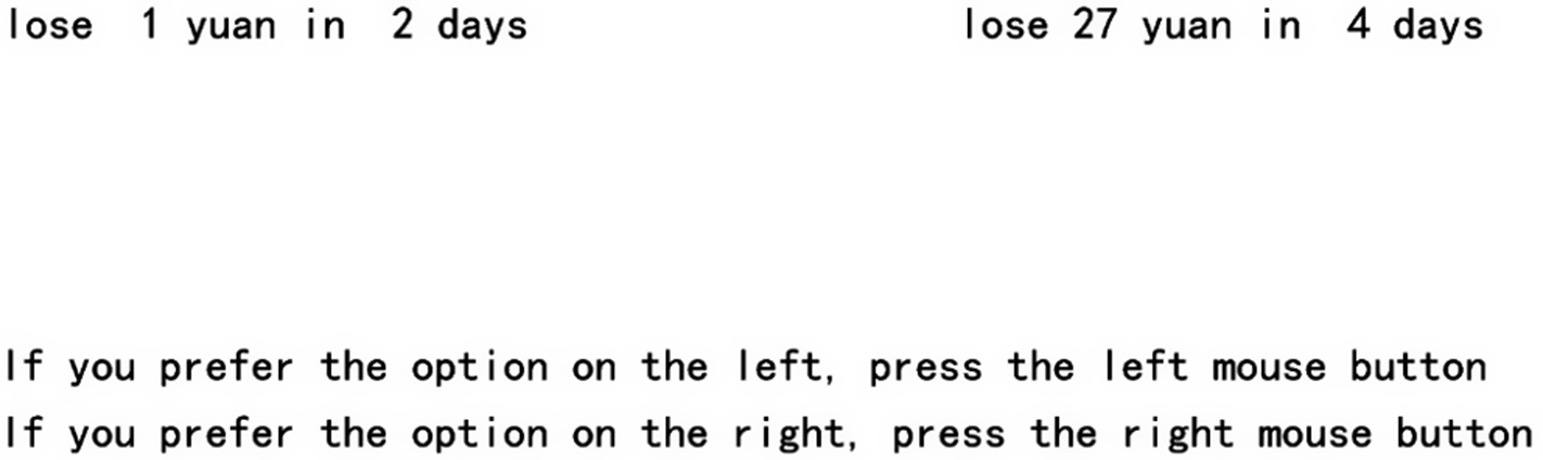
Figure 1 Screenshot of a formal choice trial in Experiment 1.
2.1.4. Data analysis
Two participants chose the dominated options in more than 1 filler trial. Therefore, their data were excluded from further analysis, and the following results were based on the data from the remaining 98 participants.Footnote 4 All the analyses in this and the following studies were conducted with a Bayesian approach using the R software (R Core Team, 2022), its rstanarm package (Goodrich et al., Reference Goodrich, Gabry, Ali and Brilleman2020) and other relevant packages. For each analysis, the default prior setting of the relevant package was adopted, and all reported results passed the convergence check (i.e., R-hat < 1.01). For the choice data in this study, we used logistic regressions to examine whether choice probabilities changed under the systematic manipulations of relevant attribute values. Specifically, the criterion variable of the logistic regressions was whether the later option was chosen, whereas the predictor variable was the rank of the manipulated attribute value for each effect, ranging from 1 (for the shortest delay or smallest loss) to 12 (for the longest delay or largest loss). As hinted above, the direction of each studied effect might differ between participants showing positive versus negative delay discounting. Therefore, for formal trials related to each effect, we first categorized them into 2 groups in terms of their suggested direction of delay discounting. Specifically, choice questions with smaller-and-sooner versus larger-and-later losses would be categorized into 1 group since they allowed for an expression of positive delay discounting. Conversely, choice questions with smaller-and-later versus larger-and-sooner losses would be categorized into the other group since they allowed for an expression of negative delay discounting. Data from the 2 groups would be analyzed separately.
For the logistic regressions, we used both the 95% credible interval (CI) of the slope parameter from the alternative model and a standard model comparison index, that is, the leave-one-out information criterion (LOOIC) to make statistical inferences. When both results favored the alternative model (i.e., when the 95% CI excluded zero and the alternative model had a lower LOOIC value than the null model), the relevant behavioral pattern would be deemed as statistically credible. In this case, we would infer that the corresponding effect existed. On the contrary, when the 95% CI of the slope parameter included zero and the null model had a lower LOOIC value, we would infer that the corresponding effect did not exist. To avoid making improper inferences about individual change patterns based on the aggregate results, we also analyzed individual data in the same way. Finally, as an exploratory analysis, we examined the variability in the direction of delay discounting both across and within participants. This would contribute to a better understanding of when and why negative discounting might occur in the loss domain.
2.2. Results
Table 1 shows, for each effect, the number of participants whose seed pairs suggested positive versus negative delay discounting, as well as the results of corresponding logistic regressions for formal choice questions derived from such seed pairs. More seed pairs suggested positive rather than negative discounting (proportion of positive discounting = 61.2%, BF10 = 124.9 given a null value of 50%). For the logistic regressions, the 95% CIs were always consistent with the LOOIC values in terms of resultant statistical inferences. It turned out that each manipulation produced a change in choice proportion no matter whether the relevant formal trials suggested positive or negative discounting.
Table 1 Results of logistic regressions on the aggregate and individual data from Experiment 1
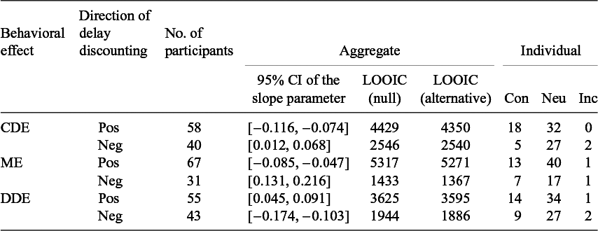
Note: CDE, common difference effect; ME, magnitude effect; DDE, delay duration effect; Pos, positive; Neg, negative; CI, credible interval; Con, consistent; Neu, neutral; Inc, inconsistent.
Specifically, when the delays of both losses were increased by the same length (i.e., the manipulation for studying the common difference effect), participants who appeared to prefer later rather than earlier losses (i.e., positive delay discounting) became more likely to choose the sooner-and-smaller loss, whereas those who appeared to prefer earlier instead of later losses (i.e., negative delay discounting) became more likely to choose the later-and-smaller loss. These opposite simple effects naturally led to an interaction effect between the suggested direction of delay discounting and the manipulation of delay length (95% CI of the regression coefficient for the interaction term = [−0.085, −0.050]).Footnote 5 Note that under the manipulation for studying the common difference effect, the smaller loss always became more bearable relative to the larger loss. The last 3 columns of Table 1 present the numbers of participants whose individual data demonstrated credibly the same change patterns as the aggregate data (i.e., consistent), no changes (i.e., neutral), or the change patterns opposite to the aggregate results (i.e., inconsistent) under the relevant manipulations. As can be seen, under either direction of delay discounting, individual data from a majority of participants showed no impact of the relevant manipulations. For those who showed credible changes, more participants demonstrated changes that were consistent with the aggregate results.
Similarly, when both loss amounts were increased proportionally (i.e., the manipulation for studying the magnitude effect), participants became more likely to choose the option with a smaller loss, which was the sooner option for participants showing positive discounting but the later option for participants showing negative discounting. These opposite simple effects again led to a credible interaction between suggested direction of delay discounting and the manipulation of loss amount (95% CI of the regression coefficient for the interaction term = [−0.143, −0.097]). The individual analysis led to similar results as those for the common difference effect: data from more participants showed credible changes that were consistent rather than inconsistent with the aggregate pattern, and a majority of individual data credibly suggested no impact of the manipulation. When the delays to both losses were increased proportionally (i.e., the manipulation for studying the delay duration effect), participants became more likely to choose the option with a larger loss, which was the later option for those showing positive discounting but the sooner option for those showing negative discounting. Like the other 2 effects, these opposite simple effects also led to a credible interaction between the suggested direction of delay discounting and the manipulation of the relevant attribute value (95% CI of the regression coefficient for the interaction term = [0.081, 0.124]). The results of individual analysis were again similar to the results regarding the other 2 effects.
Finally, for some participants, the individual seed pairs were inconsistent in terms of the implied direction of delay discounting. Specifically, seed pairs of 42 participants consistently suggested positive delay discounting, those of 19 participants consistently suggested negative delay discounting, whereas seed pairs of the remaining 37 participants did not show a consistent direction of delay discounting.
2.3. Discussion
This study was aimed at examining whether systematic changes in attribute values would lead to altered time preference in the loss domain when elicited by the choice method, presumably the most popular method in the literature. It ended up that all the manipulations led to changes in choice proportion, but the shifts in preference between the sooner and later losses depended on the direction of delay discounting implied by relevant choice questions. The finding of the common difference effect under positive discounting echoed the results of Holt et al. (Reference Holt, Green, Myerson and Estle2008), whose study design enforced positive discounting on participants. Furthermore, by allowing for negative discounting as just a few existing studies (Hardisty et al., Reference Hardisty, Appelt and Weber2013; Mitchell and Wilson, Reference Mitchell and Wilson2010) did and analyzing data from trials suggesting positive versus negative discounting separately, the current study provided clearer evidence for the conventional common difference effect under positive discounting and revealed a reverse common difference effect under negative discounting. Due to the existence of negative discounting in the loss domain and the opposite demonstrations of the common difference effect under positive versus negative discounting, it is desirable to generalize its traditional definition so that it is defined in terms of changes in the ‘absolute’ discount rate. Specifically, the common difference effect in the loss domain could be defined more properly and consistently as a decrease in absolute discount rate when both delays are increased by the same length, regardless of the direction of delay discounting. Similar definitions could be provided for the magnitude and delay duration effects.
Another critical finding of this study was that individual data from a majority of participants did not show the same credible behavioral changes as revealed in the aggregate data, and some participants even showed credibly the opposite patterns. This underlined the potential issue of blindly applying results from aggregate analysis to individual participants. Two possible causes might lead to a credible null effect at an individual level. First, the choice questions for some participants might deviate substantially from their truly indifferent pairs. As a result, the choice proportions tended to be extreme and less susceptible to the relevant manipulations. In fact, among the 50 participants for whom the 95% credible interval of regression slope for each effect covered 0, 33 participants produced choice proportions that were either above 0.95 or below 0.05. For such participants, a more appropriate set of choice questions might end up revealing an impact of the relevant manipulations. Second, the current manipulations might produce relatively small effect sizes. Since Bayesian data analysis naturally penalizes complex models more heavily, the data generated under small effect sizes could end up favoring the null hypotheses. Of course, some participants might in fact be immune to the relevant manipulations or even adopt different decision strategies leading to opposite behavioral patterns. In any case, it is more desirable to draw proper inferences from each participant’s individual data.
It was also found that, although a larger proportion of presumably indifferent seed pairs suggested positive delay discounting, a considerable share of such pairs ended up showing negative discounting. The exact proportion of empirical data that suggested negative discounting appeared to depend on the loss amount used in the relevant studies (Hardisty et al., Reference Hardisty, Appelt and Weber2013; Mitchell and Wilson, Reference Mitchell and Wilson2010), and the current proportion (i.e., 38.8%) was similar to those found in previous studies using a comparable loss amount (i.e., $10). Consequently, the current study provided further evidence for the existence of negative delay discounting in the loss domain. Furthermore, the seed pairs for an individual participant did not always suggest the same direction of delay discounting. In other words, direction of delay discounting in the loss domain might differ not only across participants but also within participants. This hinted at the roles of task factors (e.g., loss amount and delay length) in determining the direction (and probably degree) of delay discounting. However, such a result might also be produced by the instability in the discount rate revealed by the titration procedure, so further research was still needed.
3. Experiment 2
The purpose of this study was to examine whether manipulations of attribute values similar to those in Experiment 1 would lead to the same behavioral changes in time preference when elicited by a matching method. The matching method provided a straightforward way to determine the discount rate for each trial and thus facilitated the detection of behavioral effects across trials. It also helped to examine whether direction of delay discounting tended to vary within individual participants. For the same reasons as those in Experiment 1, all the trials in this study involved 2 delayed options. This experiment was pre-registered at https://osf.io/kjgv3/.
3.1. Method
3.1.1. Participants
One hundred and three students (69 females, M age = 21.2 years, SDage = 2.4 years) from a Chinese university were recruited for this study.
3.1.2. Payment schedule
The payment schedule was almost the same as that in Experiment 1, except that the base payment to the participant was 20 CNY, and the payment to the experimenter (i.e., the real loss undertaken by a participant) was determined by the participant’s response in a formal matching trial randomly picked at the end of the study. To encourage participants to always report their true matching values, the amount of the real loss was determined by the Becker–DeGroot–Marschak (BDM) mechanism (Becker et al., Reference Becker, Degroot and Marschak1964), under which reporting the true matching value was in the best interest of the participant. Take for example a trial in which the participant needed to fill in the amount of a loss in 20 days to make it as bearable as a loss of 30 CNY in 30 days. Suppose the participant indicated that he/she was indifferent between losing 25 CNY in 20 days and losing 30 CNY in 30 days. In this case, a random integer, r, would be drawn from a uniform distribution between 1 and 60 (i.e., the largest amount of loss allowed to be filled in). If r was smaller than 25 (i.e., the amount filled in by the participant), the participant should pay r CNY in 20 days. If r was greater than 25, the participant should pay 30 CNY in 30 days (i.e., the later loss). If r happened to equal 25, then the participant should pay either r CNY in 20 days or 30 CNY in 30 days with the same probability (i.e., 50%). Participants were instructed on the above procedure and told that it was in their best interest to respond according to their true preference under this mechanism. See Appendix C for the detailed instructions. On average, participants received an overall payment of 43.8 CNY in 4.1 days and paid 23.0 CNY in 39.5 days to the experimenter.
3.1.3. Materials and procedure
After granting consent to take the study, each participant first finished 5 practice trials, then completed 180 formal trials, and 10 filler trials, each requiring the participant to fill in the missing amount of a sooner loss to make it as bearable as a later loss. Specifically, in each trial, the participant is required to fill in a blank box with the missing amount and then press the Enter key to confirm his/her response (see Figure 2 for a screenshot of an exemplar trial). There were 60 formal trials designed to study each behavioral effect. The presentation order of the formal trials and the position of the sooner loss in each trial were randomized for each participant. The filled amount of the sooner loss was allowed to range between 1 and 60 CNY and the given amount of the later loss ranged between 15 and 46 CNY. The delays of the sooner losses ranged between 1 and 74 days, whereas those of the later losses ranged between 4 and 99 days. We used such ranges so that the resultant delayed losses would appear bearable to our participants and could be actually implemented. The filler trials were evenly spaced among the formal trials, and each filler trial involved 2 losses with the same delays. If the filled amount of the sooner loss differed from the given amount of the later loss, the response would be regarded as incorrect. A warning sign requesting careful responses would pop up if an incorrect response was made. Data from a participant would be excluded from further analysis if he/she responded incorrectly in more than 1 filler trial.

Figure 2 Screenshot of a formal matching trial in Experiment 2.
Table 2 shows exemplar trials of matching questions in this study. The trials regarding each behavioral effect were organized into 20 triplets. For trials regarding the common difference effect, each triplet contained 3 questions with increasingly longer delays but the same difference in delay length between each pair of losses. The 3 trials within each triplet are hereafter called short, medium, and long trials, respectively. Across different triplets, the differences in delay length ranged between 6 and 22 days, and the amounts of the later losses ranged between 20 and 40 CNY.
Table 2 Exemplar trials of matching questions in Experiment 2
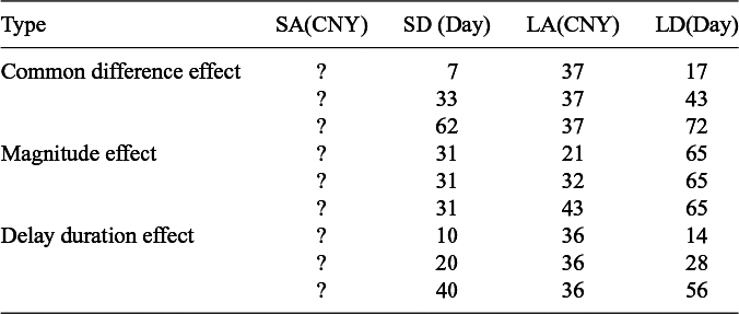
Note: Question marks indicate the missing amounts of the sooner losses. SA(SD), amount (delay) of the sooner loss; LA(LD), amount (delay) of the later loss. A filled SA value smaller/larger than the corresponding LA value indicated positive/negative delay discounting.
For trials for the magnitude effect, each triplet contained 3 questions with increasingly larger amounts of the later losses but the same shorter delays and the same longer delays. The 3 trials within each triplet are hereafter called small, medium, and large trials, respectively. Across different triplets, the shorter delays ranged between 1 and 40 days, the longer delays ranged between 22 and 99 days, and the amounts of the later losses ranged between 15 and 46 CNY.
Finally, each triplet for examining the delay duration effect contained 3 questions with increasingly longer delays but the same ratio of delay between the 2 losses in each question. The 3 trials within each triplet would also be called short, medium, and long trials, respectively, as the trials for the common difference effect. Across different triplets, the ratios of delay ranged between 2:5 and 10:11, and the amounts of the later losses ranged between 20 and 40 CNY. See Appendix D for the full list of matching questions for studying the 3 effects.
3.1.4. Data analysis
Four participants responded incorrectly in more than 1 filler trial, so their data were excluded from further analysis.Footnote 6 Therefore, all the analyses described below were based on the data from the remaining 99 participants. Before analyzing data regarding each behavioral effect, we first categorized corresponding triplets of formal trials in terms of the directions of delay discounting revealed by participants’ matching responses. Specifically, a particular triplet would be assigned to the positive/negative group if the matching values in all 3 trials indicated positive/negative delay discounting. If the trials within a triplet suggested different directions of delay discounting, the corresponding triplet would be excluded from further analysis. This setting helped to exclude trials with discount rates close to zero and thus enhanced the representativeness of remaining trials with regard to the implied direction of delay discounting. These 2 groups of triplets would then be analyzed separately to reveal potential differences in behavioral pattern between responses suggesting positive versus negative discounting.
For each group of triplets regarding a particular effect, we calculated the discount rate of each trial and performed pairwise comparisons of discount rates between the short/small, medium, and long/large trials. If the relevant manipulation had an impact on time preference, the discount rates should change monotonically with the relevant changes in attribute value. Because in most analyses the assumption of normality was violated, we used Wilcoxon signed-rank tests for pairwise comparisons. When the descriptive statistics for a particular effect changed monotonically across the 3 levels of manipulation and the Bayes factor (BF) of at least one of the pairwise comparisons favored a difference (i.e., greater than 3), we would infer that the relevant manipulation had an impact on time preference. When all BFs regarding the pairwise differences favored a null effect and at least one was smaller than 1/3, we would infer that the relevant manipulation had no impact. Finally, we checked the variability in the direction of delay discounting both across and within participants.
3.2. Results
Due to inconsistency in the implied direction of delay discounting, the categorization of triplets into either a positive or a negative discounting group led to the exclusion of 6.7%, 5.3%, and 8.7% of the triplets regarding the common difference effect, the magnitude effect, and the delay duration effect, respectively. Table 3 shows the distributional information of discount rates and the results of aggregate Bayesian tests regarding each behavioral effect separately for triplets suggesting positive versus negative discounting. For triplets suggesting positive discounting, increasing delays of both losses by the same length led to a statistically credible decrease in discount rate (i.e., the conventional common difference effect), and increasing delays of both losses proportionally resulted in a credible increase in discount rate (i.e., the conventional delay duration effect). However, increasing the amounts of the later losses credibly had no impact on discount rate (i.e., a null result of the magnitude effect).
Table 3 Distributional information of discount rates and results of aggregate Wilcoxon signed-rank tests for the 3 behavioral effects examined in Experiment 2
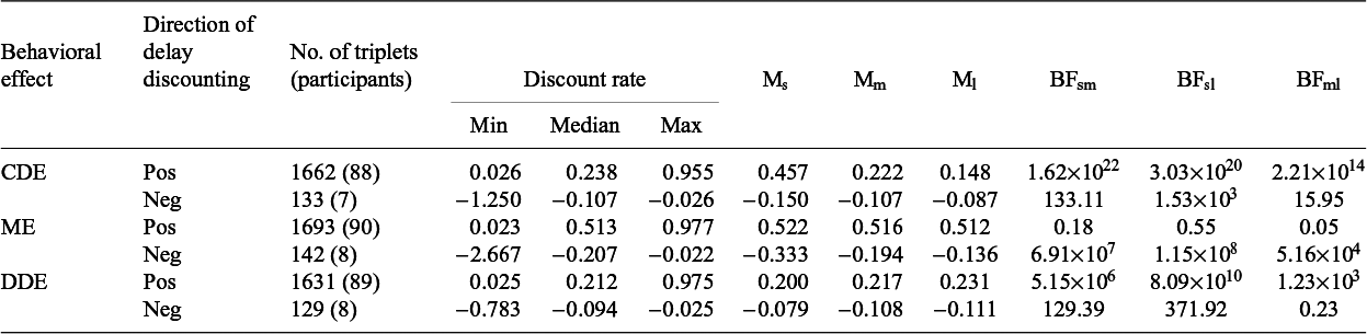
Note: CDE, common difference effect; ME, magnitude effect; DDE, delay duration effect; Pos, positive; Neg, negative; Ms, median of small/short trials; Mm, median of medium trials; Ml, median of large/long trials; BFsm, Bayes factor for the difference between the small/short and medium trials; BFsl, Bayes factor for the difference between the small/short and large/long trials; BFml, Bayes factor for the difference between the medium and large/long trials.
Corresponding individual analyses regarding the common difference and delay duration effects revealed the same statistically credible monotonic changes in discount rate as the aggregate analyses among 73 and 23 participants, respectively. In addition, data from 1 and 17 participants showed credibly no change in discount rate under the relevant manipulations. For triplets regarding the magnitude effect, individual data from 6, 17, and 1 participant showed a statistically credible decrease (i.e., the conventional magnitude effect), invariance (i.e., a null effect), and increase (i.e., the reverse magnitude effect) in discount rate, respectively.
For triplets suggesting negative delay discounting, relevant manipulations led to credible monotonic changes in discount rate regarding each studied effect at the aggregate level. Specifically, increasing delays of both losses by the same length led to an increase in discount rate (i.e., a decrease in absolute discount rate), increasing delays of both losses proportionally resulted in a decrease in discount rate (i.e., an increase in absolute discount rate), whereas increasing the amounts of the later losses led to an increase in discount rate (i.e., a decrease in absolute discount rate). The difference in simple common difference effect between positive and negative discounting triplets produced a credible interaction between the suggested direction of delay discounting and the relevant manipulation of delay length (a BF value above 109 for each pairwise comparison). The same applied to the difference in simple effect regarding the magnitude effect (a BF value above 385 for each pairwise comparison). However, the difference in simple effect regarding the delay duration effect was not credible (a BF value below 0.037 for each pairwise comparison). See Figure 3 for a graphic demonstration of the relevant patterns. Analyses of individual data revealed the same credible monotonic changes in discount rate as the aggregate results for 4, 7, and 2 participants in each of the 3 attribute value manipulation conditions, respectively. Additionally, data from 1 participant showed credibly no change in discount rate under the manipulation regarding the common difference effect.
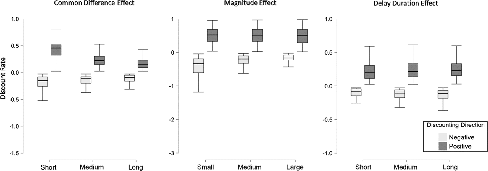
Figure 3 Discount rates under positive versus negative delay discounting and different manipulations of attribute values regarding the common difference, magnitude, and delay duration effects in Experiment 2.
Finally, quite some participants showed variable directions of delay discounting across the 180 formal trials (see Figure 4). Specifically, matching responses of 37 participants always showed positive discounting, those of 2 participants always showed negative discounting, and 60 participants showed both positive and negative delay discounting across different formal trials, with 5 participants demonstrating predominately negative discounting.
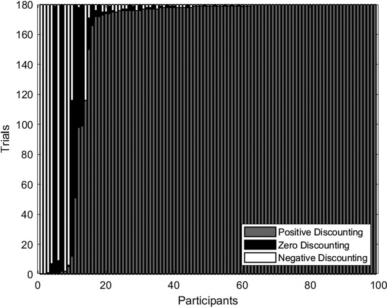
Figure 4 Distribution of formal trials with regard to the revealed direction of delay discounting for each participant in Experiment 2.
3.3. Discussion
Using a matching method with delayed losses, this study revealed nearly the same behavioral effects as those shown in Experiment 1. Specifically, at the aggregate level, almost all manipulations led to credibly monotonic changes in discount rate among categorized triplets suggesting either positive or negative delay discounting. The only exception occurred when the amounts of the later losses were manipulated and participants’ responses suggested positive delay discounting. Additionally, the change directions in discount rate, if any, differed between triplets suggesting positive versus negative discounting. As in Experiment 1, this underscored the necessity of generalizing the definitions of the 3 effects in terms of changes in ‘absolute’ discount rate. Given the well-established individual difference in the direction of delay discounting when losses are of concern, the opposite impacts also suggest that analyzing aggregate data without distinguishing between trials suggesting positive and negative discounting might produce misleading results.
As in Experiment 1, this study also showed that monotonic changes in discount rate found in aggregate data would occur to only a proportion of individual data, with data from some participants showing credibly no change or even the reverse changes. This result highlights once more that caution should be taken when applying inferences drawn from aggregate data to individual decision makers. Finally, this study revealed variable directions of delay discounting both across and within participants while using the matching method. The presence of this variability under both the choice method (i.e., Experiment 1) and the matching method suggests that it is unlikely to occur due to task-specific features but constitutes an inherent property of time preference for losses.
4. Experiment 3
This study examined time preference for losses further using an evaluation method (i.e., a special form of the matching paradigm). As hinted above, it is infeasible to investigate the common difference effect and trivial to study the delay duration effect under this method as it always involves an immediate loss for which the amount should be filled. Therefore, only the magnitude effect was examined in this study. This experiment was pre-registered at https://osf.io/8qczb/.
4.1. Method
4.1.1. Participants
One hundred students (71 females, M age = 21.6 years, SDage = 3.0 years) from a Chinese university were recruited for this study. Virtually the same payment schedule was implemented as in Experiment 2. The only exception occurred to the base payment, which was 15 CNY in this study. On average, the participants received an overall payment of 39.9 CNY in 4.1 days and paid 24.5 CNY in 31.7 days to the experimenter.
4.1.2. Materials and procedure
This study was similar to Experiment 2 in design but involved different trials. Specifically, each participant needed to finish 5 practice trials, 180 formal evaluation trials, and 10 filler trials. The formal trials were organized into 60 triplets and 3 exemplar triplets of such trials are shown in Table 4. The sooner option in each trial always occurred immediately, whereas the later options within each triplet of formal trials always had the same delays but increasingly larger amounts of losses; the corresponding trials would hereafter be called small, medium, and large trials, respectively. The amounts of delayed losses in formal trials ranged between 15 and 46 CNY and the corresponding delays ranged between 3 and 98 days. See Appendix E for the full list of to-be-evaluated options in this study.
Table 4 Exemplar triplets of formal evaluation trials in Experiment 3
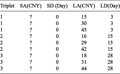
Note: Question marks indicate the missing amounts of the sooner (i.e., immediate) losses. SA(SD), amount (delay) of the sooner loss; LA(LD), amount (delay) of the later loss. A filled SA value smaller/larger than the corresponding LA value indicated positive/negative delay discounting.
4.1.3. Data analysis
Fourteen participants responded incorrectly in more than 1 filler trial, so their data were excluded from further analysis, and all the results reported below were based on the data from the remaining 86 participants. As before, we first categorized triplets of formal trials in terms of the directions of delay discounting revealed by participants’ responses. Afterward, we calculated the discount rate of each valid trial and performed separate pairwise comparisons between the small, medium, and large trials for triplets suggesting positive versus negative discounting. If manipulating the amount of the delayed loss would affect time preference, a monotonic change in discount rate should occur. As in Experiment 2, we also checked the variability in the direction of delay discounting both across and within participants.
4.2. Results
Due to inconsistency in implied direction of delay discounting, 17.3% of the formal triplets were excluded from further analysis. Table 5 shows the distributional information of discount rates and the results of aggregate Bayesian Wilcoxon signed-rank tests regarding the magnitude effect. As can be seen, for triplets suggesting either positive or negative discounting, there were credible monotonic changes in discount rate between the small, medium, and large trials. The opposite change directions again led to an interaction between the implied direction of delay discounting and the manipulation of loss amount (a BF value above 25 for each pairwise comparison). See Figure 5 for a graphic demonstration of the relevant patterns.
Table 5 Distributional information of discount rates and results of aggregate Wilcoxon signed-rank tests regarding the magnitude effect in Experiment 3
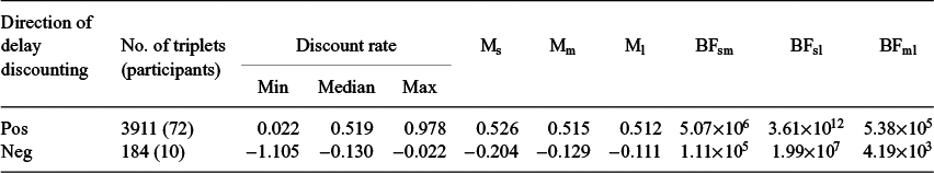
Note: Pos, positive; Neg, negative; Ms, median of small trials; Mm, median of medium trials; Ml, median of large trials; BFsm, Bayes factor for the difference between the small and medium trials; BFsl, Bayes factor for the difference between the small and large trials; BFml, Bayes factor for the difference between the medium and large trials.
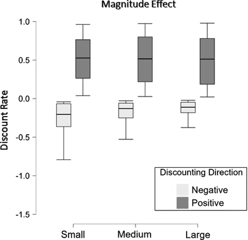
Figure 5 Discount rates under positive versus negative delay discounting when the amounts of the later losses were manipulated for studying the magnitude effect in Experiment 3.
Analyses of individual data showed that 29 and 6 participants demonstrated the same credible changes in discount rate as the aggregate data under positive and negative delay discounting, respectively. In addition, among participants who produced triplets that consistently indicated positive delay discounting, 9 participants’ evaluation responses in such triplets demonstrated credible invariance in discount rate, whereas 12 participants’ evaluation responses in such triplets showed a change pattern opposite to the aggregate result. No other participants showed credible behavioral patterns. The proportion of participants who showed a credible reverse magnitude effect under positive delay discounting (i.e., 12 out of 72) was higher than those in Experiment 1 (i.e., 1 out of 67, BF10 = 17.84) and Experiment 2 (i.e., 1 out of 90, BF10 = 92.01). Finally, evaluation responses of 58 participants demonstrated positive or no discounting, with 35 participants always showing positive discounting and 1 participant always showing no discounting. The remaining 28 participants showed negative discounting in at least some trials, with 6 participants showing predominantly negative discounting (see Figure 6).
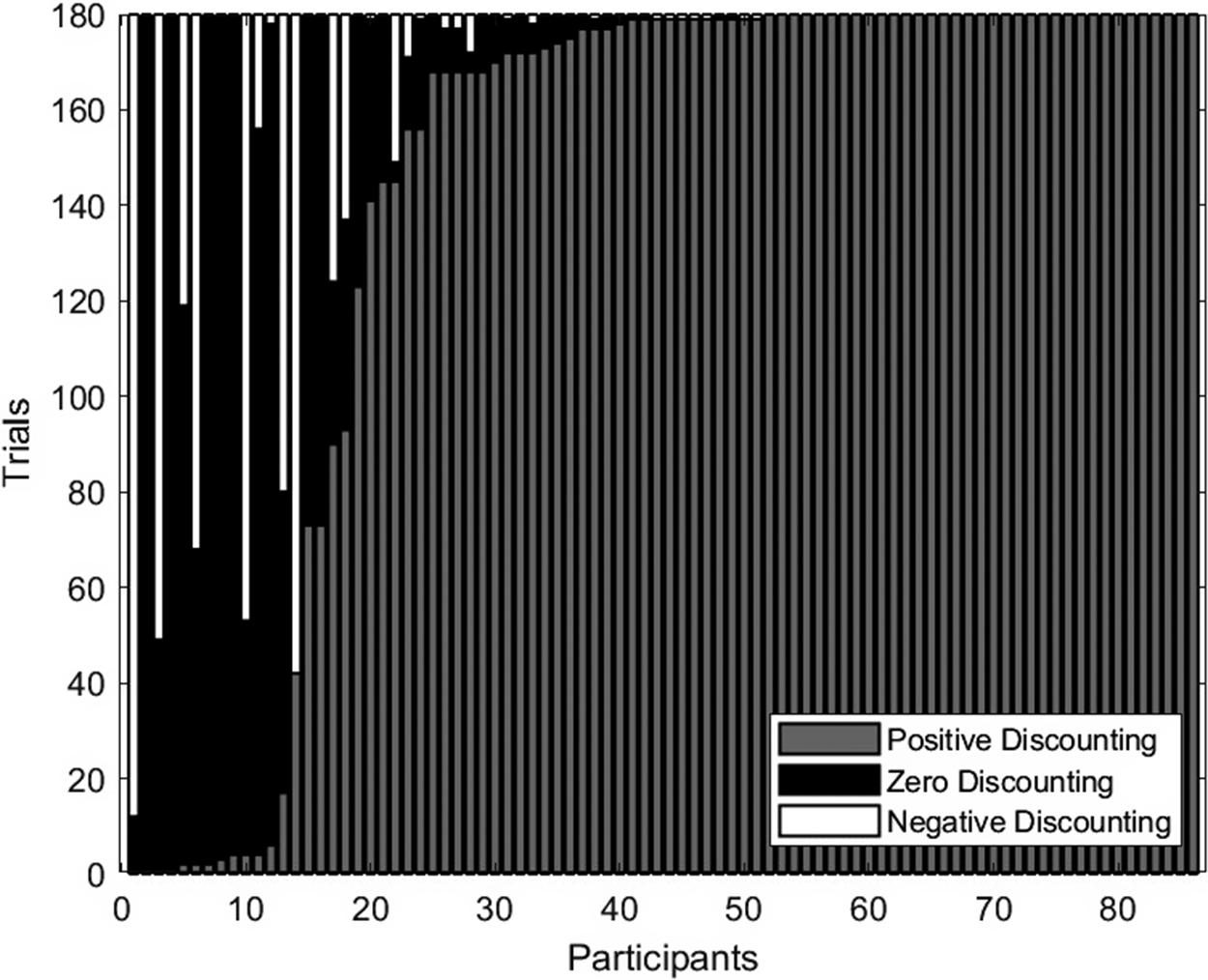
Figure 6 Distribution of formal trials with regard to the implied direction of delay discounting for each participant in Experiment 3.
4.3. Discussion
This study investigated how loss amount affected time preference elicited by an evaluation method. Aggregate data again showed opposite influences on discount rate under positive versus negative delay discounting in that discount rate tended to decrease in the former case but increase in the latter. Like in Experiment 2, which used the general matching method, this study also showed considerable individual differences in the impact of loss amount under positive delay discounting. The demonstration of the conventional magnitude effect (i.e., discount rate decreases as outcome amount increases) under positive delay discounting and its reverse under negative delay discounting (i.e., discount rate increases as outcome amount increases) could be easily accommodated by a common explanation, such as an attribute-based decision strategy. However, this strategy could not explain the finding of the reverse pattern under positive delay discounting among a considerable number of participants.
One plausible account of the above finding was provided by Hardisty et al. (Reference Hardisty, Appelt and Weber2013), that is, a preference for receiving an immediate outcome (i.e., a present bias) regardless of its valence. According to this account, people desire to resolve losses immediately, leading to a fixed bonus to the evaluation of an immediate loss relative to a delayed one. The fixed present bias would reduce the nominal discount rate of a delayed loss, and this impact would diminish as the loss amount increases, leading to the reverse behavioral pattern under positive delay discounting. Since the fixed bias applies to only immediate losses, this account emphasizes the distinctiveness of the evaluation method.
Like the previous 2 studies, the current experiment also showed that not every participant demonstrated a consistent direction of delay discounting across all formal trials. In other words, whether the participant preferred to bear a loss earlier or later seemed to vary from occasion to occasion. This further supported the possibility of variable delay discounting in terms of both degree and direction at an individual level. The above account based on a fixed present bias actually suggests a plausible mechanism for such variability, indicating the role of loss amount and delay length in determining the degree and direction of delay discounting. See General Discussion for a more quantitative analysis of this account.
5. General discussion
Intertemporal decisions in everyday life often involve negative consequences, but the majority of existing research on time preference examined only gains for an account of how people make such decisions in practice. To improve understanding of time preference in the real world, this research investigated time preference for losses using 3 different elicitation methods, that is, choice with delayed losses, matching with delayed losses, and evaluation (i.e., matching an immediate loss with a delayed one). We also analyzed data suggesting positive and negative discounting separately at both the aggregate and individual levels to draw a more refined picture. Finally, we incentivized participants by imposing real losses in the hope of eliciting more realistic preferences.
Overall, the results of the 3 experiments demonstrated consistent impacts of systematic manipulations of delay length on time preference at the aggregate level (i.e., the generalized common difference and delay duration effects in terms of changes in absolute discount rate). On the contrary, manipulation of loss amount also led to an aggregate change in discount rate under both the choice and evaluation methods but not under the general matching method. In addition, a larger proportion of participants showed the reverse magnitude effect under positive delay discounting in Experiment 3 than in the other 2 experiments, suggesting the distinctiveness of the evaluation method. It was also found that the change pattern of discount rate regarding each effect depended on the direction of delay discounting and varied across participants under each elicitation method. The finding of opposite change patterns under different directions of delay discounting underscores the importance of separating trials suggesting positive versus negative discounting while examining time preference for losses. On the contrary, this separation is practically unnecessary in the gain domain where negative discounting is rarely demonstrated.Footnote 7
The finding of individual change patterns that were neutral or even opposite to the aggregate pattern also deserves more attention. Because aggregate results might differ substantially from individual ones (e.g., Estes, Reference Estes1956; Regenwetter et al., Reference Regenwetter, Dana and Davis-Stober2011; Sidman, Reference Sidman1952), it is necessary to investigate the impacts of various types of manipulation at an individual level for a better understanding of time preference and the underlying decision strategy of each individual. For example, a somewhat surprising result in the evaluation study was that a considerable proportion of individual participants whose responses suggested positive delay discounting ended up showing the reverse magnitude effect. This finding was not only opposite to the aggregate pattern but also challenging to an attribute-based account of time preference, which was often invoked to explain the conventional magnitude effect.
One way to accommodate this individual pattern was to introduce extra components into traditional alternative-based models of time preference. For instance, present bias could be invoked to accommodate this finding in the evaluation task (Hardisty et al., Reference Hardisty, Appelt and Weber2013). Mathematically, this account suggests the following formula for the evaluation (i.e., present value) of a delayed loss with amount x < 0 and delay t,
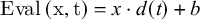 $$\begin{align}\mathrm{Eval}\left(\mathrm{x},\mathrm{t}\right)=x\cdot d(t)+b\end{align}$$
in which d(t) represents a multiplicative discount factor as a function of delay and b < 0 indicates a fixed present bias. This bias made it more bearable to take a loss immediately rather than later. The nominal discount rate of the delayed loss would then be
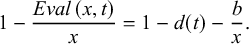 $$\begin{align*}1-\frac{Eval\left(x,t\right)}{x}=1-d(t)-\frac{b}{x}.\end{align*}$$
It is readily seen that the nominal discount rate would approach 1 – d(t) as the absolute value of x increases, leading to the reverse magnitude effect. When d(t) is small and x is large, the nominal discount rate would be positive, providing a complete account of the reverse magnitude effect found under positive delay discounting. Conversely, when d(t) is large and x is small, the nominal discount rate could be negative, leading to the reverse magnitude effect under negative discounting. Overall, Equation (1) provides a unified account of the reverse magnitude effects found under both positive and negative delay discounting. It can also explain the variability in discount rate both across and within participants, when b serves as a personal variable and t and x serve as situational variables.
However, to account for the conventional magnitude effect found among some participants whose responses suggested positive delay discounting, one still needs to assume a multiplicative discount factor depending on both the delay length and loss amount, an additive discounting function, or attribute-based decision strategies. Consequently, the mixed findings of both Experiments 2 and 3 suggested that distinct strategies or factors are considered by different people while processing a delayed loss. The existence of immediate losses appeared to further diversify people’s strategies for determining relevant time preference. Note that such findings are only possible when trials suggesting positive versus negative discounting are separately analyzed at an individual level.
5.1. Accommodation of existing research
The general finding of opposite impacts of loss amount under positive versus negative delay discounting and the results regarding distinct decision strategies also help to reconcile contradictory findings of previous studies examining the magnitude effect in the loss domain. Specifically, although some studies revealed the conventional magnitude effect (e.g., Anvari et al., Reference Anvari, Verdeş and Marchiori2022) or no systematic impact of loss amount on the degree of discounting (e.g., Baker et al., Reference Baker, Johnson and Bickel2003; Mitchell and Wilson, Reference Mitchell and Wilson2010), Hardisty et al. found the reverse magnitude effect. Three facts regarding the relevant research design might contribute to these inconsistent results. First, different elicitation methods were employed in these studies: Anvari et al. (Reference Anvari, Verdeş and Marchiori2022) adopted a differential method in which the participants were required to report either the absolute or relative increase in loss amount to make a delayed loss equally bearable to a given immediate loss; Baker et al. (Reference Baker, Johnson and Bickel2003) used a choice-based titration procedure with immediate and delayed losses, whereas Mitchell and Wilson (Reference Mitchell and Wilson2010) and Hardisty et al. (Reference Hardisty, Appelt and Weber2013) used fixed lists of choice questions to investigate the effect. The method adopted by Anvari et al. was likely to induce an attribute-based approach to such a decision and thus facilitate a conventional magnitude effect.
Second, these studies allowed different degrees of negative discounting to be expressed: Hardisty et al. allowed participants to express negative delay discounting to a substantial extent, whereas in the other studies expression of negative discounting was either disallowed (e.g., Anvari et al., Reference Anvari, Verdeş and Marchiori2022; Baker et al., Reference Baker, Johnson and Bickel2003) or could only assume a very low degree (Mitchell and Wilson, Reference Mitchell and Wilson2010). Allowing for an expression of negative discounting could favor the reverse magnitude effect as shown in the current research. Finally, all these studies analyzed data suggesting positive versus negative discounting (if allowed) together. Consequently, the overall results would depend on the proportion of participants who preferred earlier rather than later losses, leading to apparently contradictory results from different studies.
Similar analysis also applies to the existing studies on the common difference effect. Allowing for only positive delay discounting, Holt et al. (Reference Holt, Green, Myerson and Estle2008) found the conventional common difference effect just as our studies did under the same condition. Recent studies by Furrebøe (Reference Furrebøe2020a, Reference Furrebøe2020b) adopted a similar design and revealed the same pattern. Given the results of the current research, it is likely that the conventional common difference effect would be reversed if participants had been allowed to express negative delay discounting. In summary, the current research emphasizes the critical value of allowing for an expression of negative discounting and analyzing data suggesting positive versus negative discounting separately for a better understanding of time preference for losses.
5.2. Caveats and future directions
One important finding of the current research was that inconsistent directions of delay discounting might even show up at an individual level. One possible explanation was an unreliable measurement of discount rate. To prevent such a possibility, we have taken multiple measures in the current research, including filler trials to detect and warn against inattentive responses, a titration procedure allowing for probabilistic choices, and real incentives to facilitate expression of true preference. Given all these measures, it was unlikely that inconsistent directions of discounting were produced by inattentive or random responses. However, future research should try more reliable measures of discount rate or relevant indices to further validate the current results. Alternatively, this apparent inconsistency might reflect something inherent in time preference for losses, and the direction of delay discounting might actually depend on factors such as delay length and loss amount. This possibility was predicted by existing theories considering present bias (e.g., Benhabib et al., Reference Benhabib, Bisin and Schotter2010; Hardisty et al., Reference Hardisty, Appelt and Weber2013) and suggested by recent theoretical and empirical work (Scholten et al., Reference Scholten, Walters, Fox and Read2024). More research is needed to further examine such dependency for a better understanding of time preference for losses.
Consistent with existing studies that allowed for an expression of negative delay discounting, the current research also revealed reliable instances of negative delay discounting among a proportion of participants. Previous studies have shown that some people might prefer to bear losses earlier rather than later when it was possible to get rid of losses immediately, as if they were aversive to debt or had a ‘let’s get it over with’ attitude. Such a tendency is only possible for a choice between an immediate loss and a delayed loss, the typical pair of options examined in the literature (e.g., Hardisty et al., Reference Hardisty, Appelt and Weber2013; Thaler, Reference Thaler1981). The current study extended the previous finding in that the same preference was also demonstrated when the elicitation method involved 2 delayed losses. In this case, both options could be interpreted as debts and the explanation based on debt aversion or a ‘let’s get it over with’ attitude became less relevant. It appeared that some people just had a general preference to resolve losses as early as possible, no matter whether this goal could be fulfilled immediately or at a shorter delay. Future research should examine potential psychological factors contributing to this negative delay discounting, such as the negative anticipatory utility generated by delayed losses (Hardisty and Weber, Reference Hardisty and Weber2020; Loewenstein, Reference Loewenstein1987).
Data availability statement
Data and materials are available at https://osf.io/ur62e/.
Funding statement
This research was supported by a grant from the National Natural Science Foundation of China to J.D. (Grant No. 31872780).
Competing interests
There are no relevant financial or non-financial competing interests to report.
Appendix A
The titration procedure for generating seed pairs in Experiment 1
To generate formal choice questions for examining each behavioral effect, we first implemented a titration procedure to find 3 seed pairs of approximately equally bearable losses for each participant. The titration procedure involved sequences of choice questions for finding the seed pairs. For example, to find the seed pair for examining the common difference effect, the titration procedure would ask participants to choose between a loss with a variable amount in 20 days and a loss of a fixed amount of 28 CNY in 80 days. In the first 2 questions, the variable amounts of the sooner loss were set to be 1 and 49 CNY, respectively. Note that losing 49 CNY in 20 days was obviously inferior to losing 1 CNY in 20 days, so, given transitivity of preference, nobody should have chosen the later option in the first question but the sooner option in the second question. It ended up that none of the participants showed this irrational choice pattern.
Other possible combinations of responses to these 2 questions involved choosing the sooner options in both questions, the later options in both questions, and the sooner option in the first question but the later option in the second. Choosing the sooner options in both questions suggested a high degree of negative delay discounting. Given the allowed range of loss amounts in the formal choice questions (i.e., between 1 and 49 CNY), the seed pair in this case would be set to contain an option of losing 49 CNY in 20 days and the other option of losing 28 CNY in 80 days. Conversely, choosing the later options in both questions suggested a high degree of positive delay discounting. Consequently, the seed pair would be set to contain an option of losing 1 CNY in 20 days and the other option of losing 28 CNY in 80 days.
Finally, a participant might choose the sooner option when its amount was smaller (i.e., 1 CNY) but the later option when its amount was larger (i.e., 49 CNY). This pattern suggested that the indifferent amount of the sooner option shall lie between 1 and 49 CNY. Therefore, a choice question between losing 25 CNY in 20 days and losing 28 CNY in 80 days would be presented, and the titration procedure would proceed to adjust the variable amount of the sooner loss to approach this indifferent amount. Specifically, the variable amount would be increased if the sooner option was chosen but decreased when the later option was chosen. A pair of limits on the variable amount was used for this purpose, with respective initial values of 1 (i.e., the lower limit) and 49 CNY (i.e., the upper limit). Choosing the sooner option would result in an upward adjustment of the lower limit, whereas choosing the later option would result in a downward adjustment of the upper limit. To accommodate probabilistic choices, the adjustment was partial in the sense that the updated limit was a weighted average of the present limit and the current amount of the sooner loss, with 10% and 90% as the weights. With the updated limit, the variable amount of the sooner loss in the next choice question would be set to be the average of the lower and upper limits.
This procedure would continue until the difference between the lower and upper limits was no larger than 2 CNY. Note that the variable amount of the sooner loss was always rounded to the nearest integer and shown accordingly. Also, note that some participants may demonstrate a very low degree of delay discounting, whereby the indifferent amount was close to the fixed amount of the later loss. In this case, a choice question between losing 28 CNY in 20 days and losing 28 CNY in 80 days would be presented. If a participant chose the sooner option, indicating positive delay discounting, then the seed pair would be set to contain an option of losing 27 CNY in 20 days and the other option of losing 28 CNY in 80 days. Otherwise, the seed pair would be set to contain an option of losing 29 CNY in 20 days and the other option of losing 28 CNY in 80 days, since choosing the later option suggested negative delay discounting.
Similar procedures were used to generate seed pairs for examining the magnitude effect and the delay duration effect. The questions regarding the magnitude effect would involve a loss of 31 CNY with a variable delay and a loss of 34 CNY in 50 days, whereas those regarding the delay duration effect would involve a loss in 21 days with a variable amount and a loss of a fixed amount of 27 CNY in 53 days. With the 3 seed pairs of approximately equally bearable losses for each participant, the experiment program would then generate 12 unique choice questions for examining each behavioral effect.
Appendix B
List of choice questions for an exemplar participant in Experiment 1
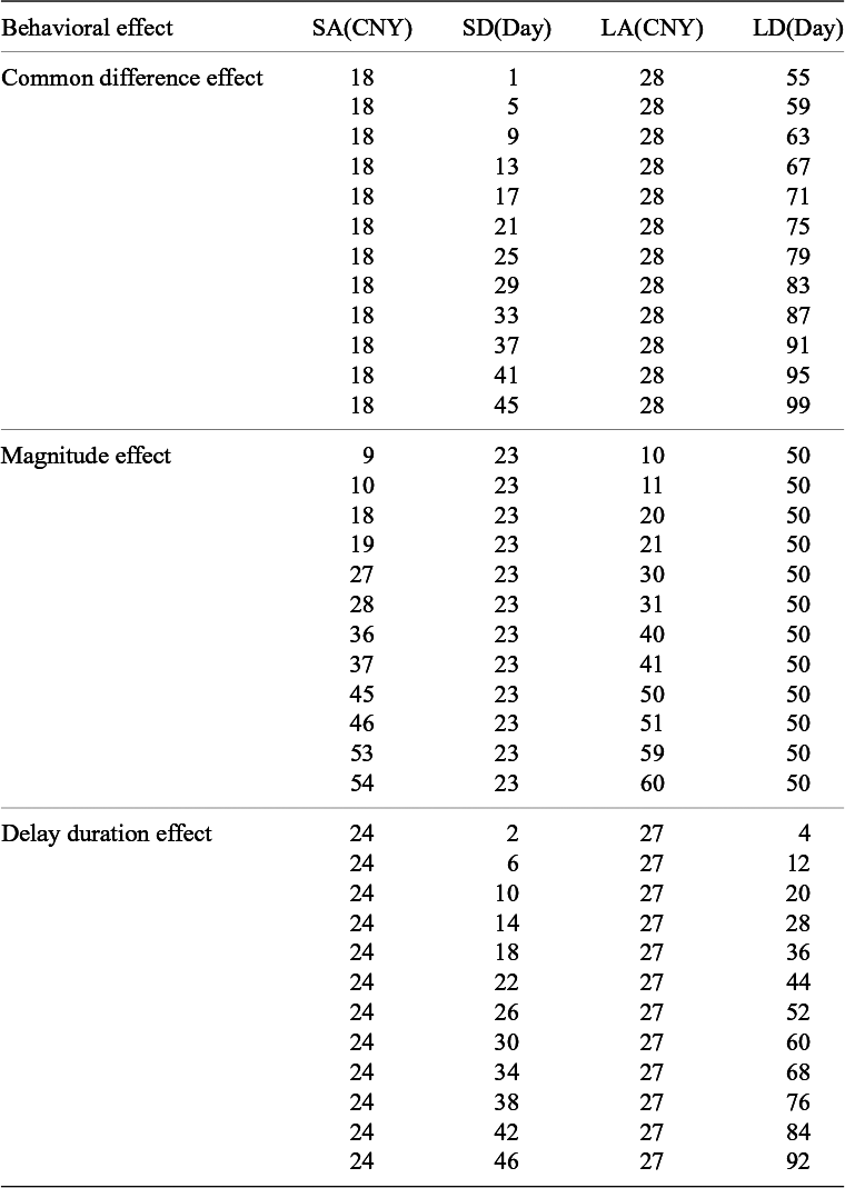
Note: SA(SD), amount (delay) of the sooner loss; LA(LD), amount (delay) of the later loss. For this participant, all choice questions implied positive delay discounting.
Appendix C
Details of the BDM procedure used in Experiments 2 and 3
In both Experiment 2 (i.e., the matching study) and Experiment 3 (i.e., the evaluation study), the BDM mechanism was adopted to encourage participants to report their true matching values. In each case, a random integer, x, would be drawn from a uniform distribution between 1 and 60 (i.e., the largest amount of loss allowed to be filled in) and then compared with the filled amount of the sooner loss to determine the amount and delay of the real loss. Following is an illustrative instruction provided in Experiment 2.
To provide a real incentive for the experiment, the computer program would randomly select a decision problem you have encountered and determine accordingly the amount and delay of the loss you need to bear.
For example, suppose the randomly selected problem asks how much loss in 20 days would be equivalent to losing 30 CNY in 30 days, and you put 25 CNY as your response in the experiment. In this case, the program would pick a random number, x, between 1 and 60 (the upper limit in the experiment).
If x is larger than your response (i.e., x > 25), you shall pay 30 CNY in 30 days.
If x is smaller than your response (i.e., x < 25), you shall pay x CNY in 20 days.
If x is equal to your response (i.e., x = 25), you shall either pay 30 CNY in 30 days or pay 25 CNY in 20 days.
The above rule is set to encourage you to adjust the missing value so that the resultant pair of losses are equally bearable according to your true preference. It can be proved mathematically that reporting according to your true preference is in your best interest under this rule.
Appendix D
List of formal matching questions in Experiment 2
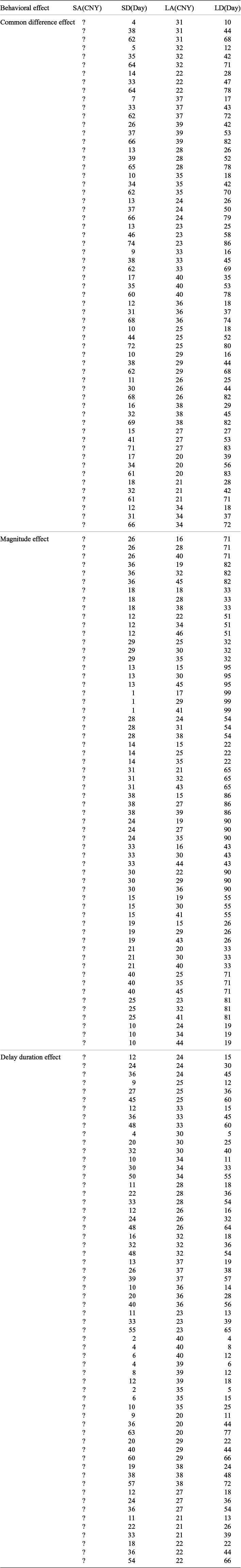
Note: SA(SD), amount (delay) of the sooner loss; LA(LD), amount (delay) of the later loss. Question marks indicate the missing attribute values to be filled in.
Appendix E
List of to-be-evaluated options regarding the magnitude effect in Experiment 3
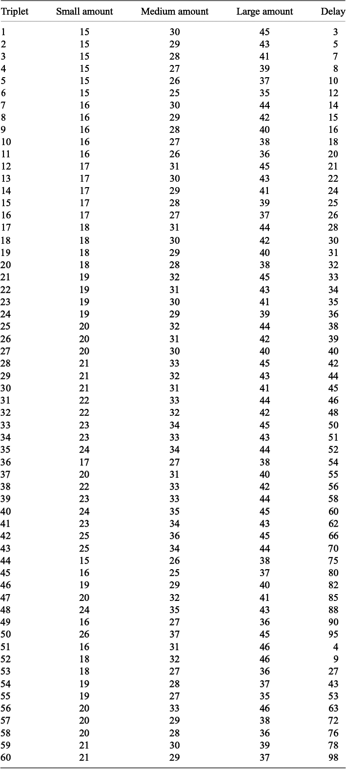
Note: Amounts were shown in the unit of CNY and delays were shown in the unit of day.


 Open access